Limits of Feedback and RHP

8/6/2019 Limits of Feedback and RHP

http://slidepdf.com/reader/full/limits-of-feedback-and-rhp 1/29

Limits of Feedback ControlRegeltechniek 2, 5K120

Regeltechniek VKO, verkorte opleiding, 5F120

Ad Damen

Measurement and Control group

Department of Electrical Engineering

Eindhoven University of Technology

P.O.Box 513

5600MB Eindhoven

E-mail: [email protected]

Version of July 25, 2003



2



Contents

0.1 Stability

Usually the first prerequisite for the closed loop is stability, so that we start analysing thisaspect.

0.1.1 Pole zero cancellation in the RHP

In this subsection it will be demonstrated that feedback is indispensable for stabilisation.From a practical point of view this is easy to understand: if you want to stabilise an

inverted pendulum, you have to observe in what direction it tends to fall.However, if one is focussed too much on the algebraic equations and forget about the

link to practice, one can easily get trapped into tricky reasonings as simple feedforwardwith pole zero cancellations.

For the demonstration of pole-zero compensation effects we will take a plant transfer:

P =s − 1

s − 2(0.1)

Algebraically we can annihilate both zero and pole at the Right Half Plane (RHP) bytaking as a compensator:

C = s − 2s − 1 (0.2)

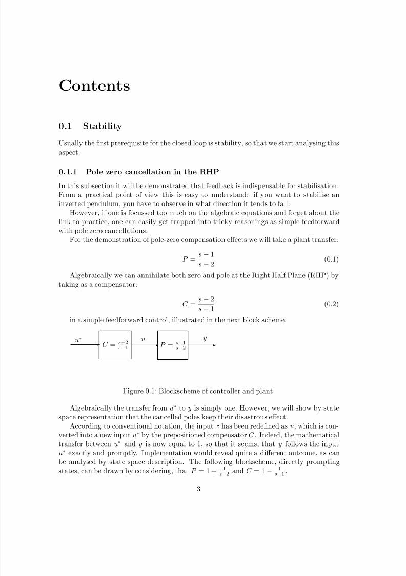
in a simple feedforward control, illustrated in the next block scheme.

C = s−2s−1 P = s−1

s−2- - -u∗ u y

Figure 0.1: Blockscheme of controller and plant.

Algebraically the transfer from u∗ to y is simply one. However, we will show by statespace representation that the cancelled poles keep their disastrous effect.

According to conventional notation, the input x has been redefined as u, which is con-verted into a new input u∗ by the prepositioned compensator C . Indeed, the mathematicaltransfer between u∗ and y is now equal to 1, so that it seems, that y follows the inputu∗ exactly and promptly. Implementation would reveal quite a different outcome, as canbe analysed by state space description. The following blockscheme, directly promptingstates, can be drawn by considering, that P = 1 + 1

s−2 and C = 1− 1s−1 .

3



1s

1s

1

1

- - - - -- - 6

-

?6

-

?

6

?

6

u∗ x1 u x2 x2 y

C P

−1- -

? 2

x1

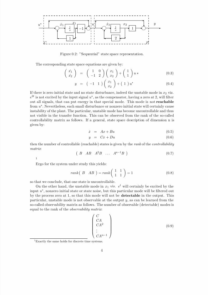
Figure 0.2: ”Sequential” state space representation.

The corresponding state space equations are given by:x1x2

=

1 0−1 2

x1x2

+

11

u ∗ (0.3)

y = −1 1

x1x2

+

1

u∗ (0.4)

If there is zero initial state and no state disturbance, indeed the unstable mode in x2 viz.e2t is not excited by the input signal u∗, as the compensator, having a zero at 2, will filter

out all signals, that can put energy in that special mode. This mode is not reachablefrom u∗. Nevertheless, each small disturbance or nonzero initial state will certainly causeinstability of the plant. The particular, unstable mode has become uncontrollable and thusnot visible in the transfer function. This can be observed from the rank of the so-calledcontrollability matrix as follows. If a general, state space description of dimension n isgiven by:

x = Ax + Bu (0.5)

y = Cx + Du (0.6)

then the number of controllable (reachable) states is given by the rank of the controllability

matrix :

B AB A

2

B . . . A

n

−1

B

(0.7)1

Ergo for the system under study this yields:

rank

B AB

= rank

1 11 1

= 1 (0.8)

so that we conclude, that one state is uncontrollable.On the other hand, the unstable mode in x1 viz. et will certainly be excited by the

input u∗, nonzero initial state or state noise, but this particular mode will be filtered outby the process zero at 1, so that this mode will not be detectable in the output. Thisparticular, unstable mode is not observable at the output y, as can be learned from theso-called observability matrix as follows. The number of observable (detectable) modes isequal to the rank of the observability matrix :⎛

⎜⎜⎜⎜⎜⎝

C CACA2

...CAn−1

⎞⎟⎟⎟⎟⎟⎠

(0.9)

1Exactly the same holds for discrete time systems.

4



1

Ergo for the system under study this yields:

rank

C CA

= rank

−1 1−2 2

= 1 (0.10)

so that we conclude that one state is unobservable.

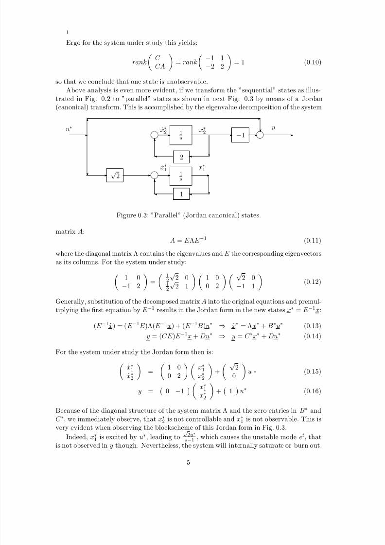
Above analysis is even more evident, if we transform the ”sequential” states as illus-trated in Fig. 0.2 to ”parallel” states as shown in next Fig. 0.3 by means of a Jordan(canonical) transform. This is accomplished by the eigenvalue decomposition of the system

1s

2

1s

1

√2

-

?

6

- -

?

6

- - ?

-

6u∗ x∗2 x∗2

x∗1 x∗1

y−1- - -

-

?

Figure 0.3: ”Parallel” (Jordan canonical) states.

matrix A:

A = E ΛE −1 (0.11)

where the diagonal matrix Λ contains the eigenvalues and E the corresponding eigenvectorsas its columns. For the system under study:

1 0

−1 2 =

12

√2 0

12√2 1 1 0

0 2

√2 0

−1 1 (0.12)

Generally, substitution of the decomposed matrix A into the original equations and premul-tiplying the first equation by E −1 results in the Jordan form in the new states x∗ = E −1x:

(E −1x) = (E −1E )Λ(E −1x) + (E −1B)u∗ ⇒ x∗ = Λx∗ + B∗u∗ (0.13)

y = (CE )E −1x + Du∗ ⇒ y = C ∗x∗ + Du∗ (0.14)

For the system under study the Jordan form then is:

x∗1x∗2

=

1 00 2

x∗1x∗2

+

√2

0

u ∗ (0.15)

y =

0 −1 x∗1

x∗2

+

1

u∗ (0.16)

Because of the diagonal structure of the system matrix Λ and the zero entries in B∗ andC ∗, we immediately observe, that x∗2 is not controllable and x∗1 is not observable. This isvery evident when observing the blockscheme of this Jordan form in Fig. 0.3.

Indeed, x∗1 is excited by u∗, leading to√ 2u∗

s−1 , which causes the unstable mode et, thatis not observed in y though. Nevertheless, the system will internally saturate or burn out.

5



Also, the unstable state x∗2 is theoretically not excited by input u∗, but any nonzero, initial

state x∗2(0) (or some noise) will lead tox∗2(0)

s−2 , so an unstable mode x∗2(0)e2t.

Consequently, the main conclusion to be drawn from this example is, that the inter-nal behaviour of a realisation (state space) may be more complicated than is indicatedby the mathematical, external behaviour (transfer function). The internal behaviour isdetermined by the natural frequencies of the (undriven) realisation, which in our case ares = 1, 2. However, because of cancellation, not all the corresponding modes of oscillation

will appear in the overall transfer function. Or, to put it another way, since the transferfunction is defined under zero initial conditions, it will not display all the modes of theactual realisation of the system. For a complete analysis, we shall need to have good waysof keeping track of all the modes, those explicitly displayed in the transfer function andalso the ”hidden” ones. It is possible to do this by careful bookkeeping with the trans-fer function calculations, but actually it was the state equation analysis as in the aboveexample, that first clarified these and related questions. It directly shows, that pole zerocancellation in the right half plane, thus of unstable poles, is strictly forbidden, as it onlymakes these unstable modes or states either uncontrollable or unobservable, but they willstill damage the nice theoretical transfer, as these signals grow uncontrollably withoutbounds.

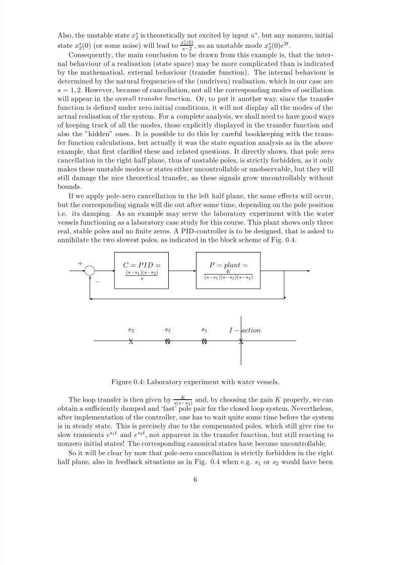
If we apply pole-zero cancellation in the left half plane, the same effects will occur,but the corresponding signals will die out after some time, depending on the pole positioni.e. its damping. As an example may serve the laboratory experiment with the watervessels functioning as a laboratory case study for this course. This plant shows only threereal, stable poles and no finite zeros. A PID-controller is to be designed, that is asked toannihilate the two slowest poles, as indicated in the block scheme of Fig. 0.4.

C = P ID =(s−s1)(s−s2)

s

P = plant =K

(s−s1)(s−s2)(s−s3)- - - -

?

6

+

−

XXOXOX

s3 s2 s1 I − action

Figure 0.4: Laboratory experiment with water vessels.

The loop transfer is then given by K s(s−s3) and, by choosing the gain K properly, we can

obtain a sufficiently damped and ‘fast’ pole pair for the closed loop system. Nevertheless,after implementation of the controller, one has to wait quite some time before the systemis in steady state. This is precisely due to the compensated poles, which still give rise toslow transients es1t and es2t, not apparent in the transfer function, but still reacting tononzero initial states! The corresponding canonical states have become uncontrollable.

So it will be clear by now that pole-zero cancellation is strictly forbidden in the righthalf plane, also in feedback situations as in Fig. 0.4 when e.g. s1 or s2 would have been

6



unstable poles.

What about poles on the imaginary axis?

On the imaginary axis the modes, corresponding to the poles, manifest themselves asundamped oscillations of undefined amplitude depending on noise or initial conditions.Consequently there are not prone for cancellation. E.g. an integrator (1/s) cascaded bya differentiator (s) shows this effect for frequency zero. These cascaded blocks producemathematically the transfer s/s = 1, but a DC-value will not pass.

Ergo the general rule becomes:no pole-zero cancellation is allowed in the closedRHP (”closed” meaning: inclusive the imaginary axis).

From now on we will assume, that all systems, to be observed and/or controlled, areboth (completely) observable and (completely) controllable and that the dimension n of the state vector is minimal, i.e. a minimal realisation.

Now we have shown, that compensation is not the way to get rid of right half planezeros and poles, the question arises how then to cope with them. Feedback can solve theproblem as explained in the next subsection. That is to say, the poles can be shifted tothe left half plane by feedback, but the zeros will stay. Zeros in the right half plane, i.e.nonminimum phase zeros, cause ineffective response: initially the response is in the wrongdirection (opposite sign). Furthermore, the rootloci end in zeros, so that these rootloci

are drawn towards the unstable, right half plane. It will lateron appear that nonminimumphase zeros put fundamental bounds on the obtainable bandwidth of closed loop systems.Consequently, what means are there to eliminate the nonminimum phase zeros? Theanswer has to be sought in the system itself comprising plant, sensors and actuators. Byproper choice and positioning of actuators and sensors, the occurrence and position of zeros can be corrected up to a high degree. If this is not sufficient, the plant itself shouldbe changed. Transfer blocks parallel to the original transfer will completely change thezeros, but this requires a fundamental redesign of the plant itself. So it advocates theprinciple of negotiating about the building of plant in the very early stage of design inorder to guarantee, that an efficient and optimal control is possible lateron!

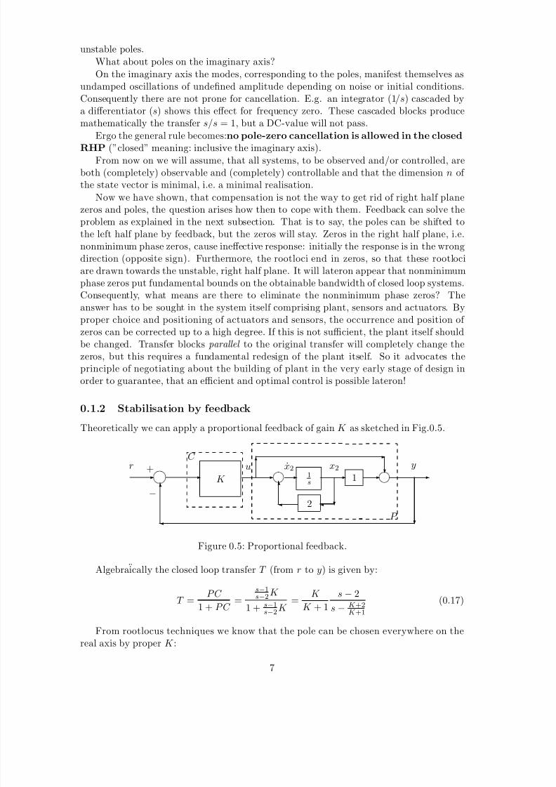
0.1.2 Stabilisation by feedbackTheoretically we can apply a proportional feedback of gain K as sketched in Fig.0.5.

1s

1- - - - - 6

-

?

?

6

u x2 x2 y

P

2

K

C

- -

?

6

r +

−

Figure 0.5: Proportional feedback.

Algebraically the closed loop transfer T (from r to y) is given by:

T =P C

1 + P C =

s−1s−2K

1 + s−1s−2K

=K

K + 1

s − 2

s − K +2K +1

(0.17)

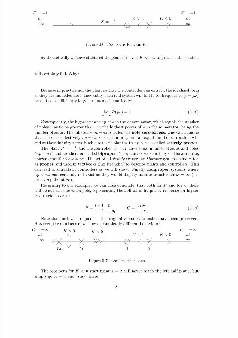
From rootlocus techniques we know that the pole can be chosen everywhere on thereal axis by proper K :

7



K > 0 K < 0K = −1

at∞

K = −1at−∞ K = −2

Figure 0.6: Rootlocus for gain K .

So theoretically we have stabilised the plant for −2 < K < −1. In practice this control

will certainly fail. Why?

Because in practice nor the plant neither the controller can exist in the idealised formas they are modelled here. Inevitably, each real system will fail to let frequencies (s = jω)pass, if ω is sufficiently large, or put mathematically:

limω

→∞

P ( jω) = 0 (0.18)

Consequently, the highest power np of s in the denominator, which equals the numberof poles, has to be greater than nz, the highest power of s in the numerator, being thenumber of zeros. The difference np−nz is called the pole zero excess. One can imaginethat there are effectively np − nz zeros at infinity and an equal number of rootloci willend at these infinity zeros. Such a realistic plant with np > nz is called strictly proper.

The plant P = s−1s−2 and the controller C = K have equal number of zeros and poles

”np = nz” and are therefore called biproper. They can not exist as they still have a finite,nonzero transfer for ω = ∞. The set of all strictly proper and biproper systems is indicatedas proper and used in textbooks (like Franklin) to describe plants and controllers. Thiscan lead to unrealistic controllers as we will show. Finally, nonproper systems, wherenp < nz can certainly not exist as they would display infinite transfer for ω =

∞(i.e.

nz − np poles at ∞).

Returning to our example, we can thus conclude, that both for P and for C therewill be at least one extra pole, representing the roll off in frequency response for higherfrequencies, so e.g.:

P =s− 1

s− 2

p1s + p1

C =Kp2

s + p2(0.19)

Note that for lower frequencies the original P and C transfers have been preserved.However, the rootlocus now shows a completely different behaviour:

K > 0 K < 0

K = −∞

at∞

K = −∞

at−∞K < 0K > 0

p2 p1 1 2

Figure 0.7: Realistic rootlocus

The rootlocus for K < 0 starting at s = 2 will never reach the left half plane, butsimply go to +∞ and ”stay” there.

8



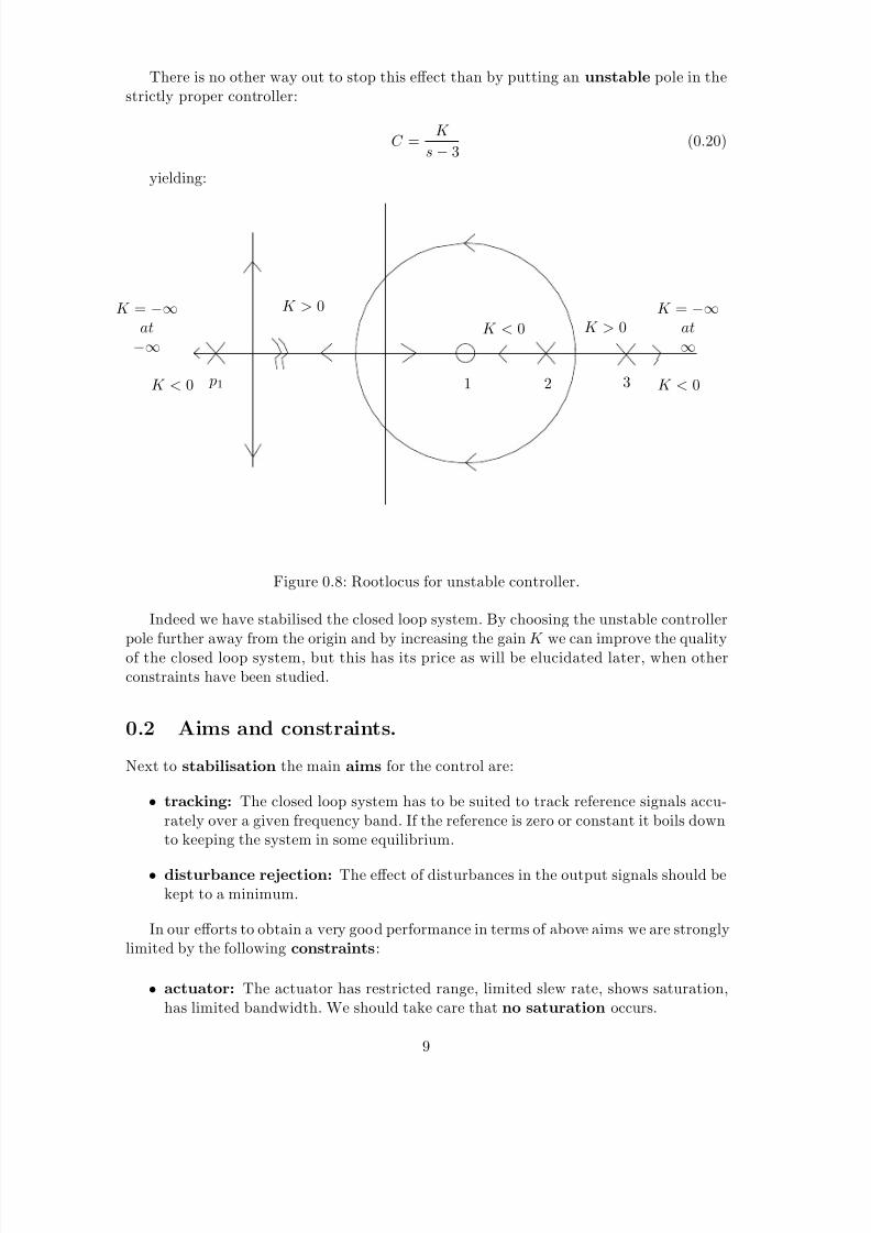
There is no other way out to stop this effect than by putting an unstable pole in thestrictly proper controller:

C =K

s − 3(0.20)

yielding:

K < 0 K > 0K = −∞

at∞

K = −∞at−∞

K < 0

K > 0

K < 0 p1 1 2 3

Figure 0.8: Rootlocus for unstable controller.

Indeed we have stabilised the closed loop system. By choosing the unstable controllerpole further away from the origin and by increasing the gain K we can improve the qualityof the closed loop system, but this has its price as will be elucidated later, when otherconstraints have been studied.

0.2 Aims and constraints.

Next to stabilisation the main aims for the control are:

• tracking: The closed loop system has to be suited to track reference signals accu-rately over a given frequency band. If the reference is zero or constant it boils downto keeping the system in some equilibrium.

• disturbance rejection: The effect of disturbances in the output signals should bekept to a minimum.

In our efforts to obtain a very good performance in terms of above aims we are stronglylimited by the following constraints:

• actuator: The actuator has restricted range, limited slew rate, shows saturation,has limited bandwidth. We should take care that no saturation occurs.

9



• sensor: The sensor may be very accurate, it will always contribute measurement

noise and it is not feasible to strive for a controlled accuracy higher than the sensorallows. Furthermore, if the sensor is not sufficiently broadbanded, this defect shouldinfluence controller design.

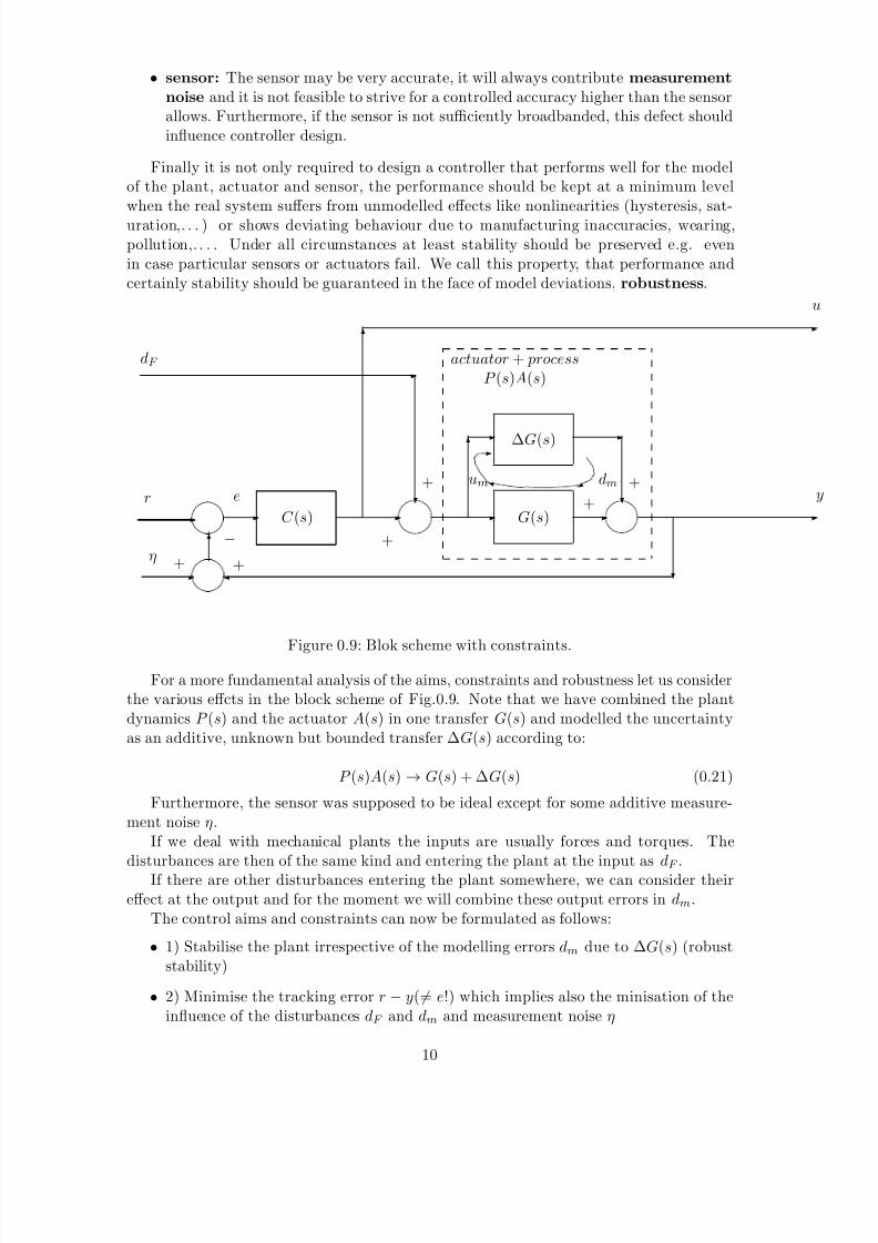
Finally it is not only required to design a controller that performs well for the modelof the plant, actuator and sensor, the performance should be kept at a minimum levelwhen the real system suffers from unmodelled effects like nonlinearities (hysteresis, sat-uration,. . . ) or shows deviating behaviour due to manufacturing inaccuracies, wearing,pollution,. . . . Under all circumstances at least stability should be preserved e.g. evenin case particular sensors or actuators fail. We call this property, that performance andcertainly stability should be guaranteed in the face of model deviations, robustness.

G(s)

ΔG(s)

- -

6- -

?

actuator + processP (s)A(s)

-y

u

C (s)

?

6

-

-η

++

−-

e

6-

-

?

dF

+

+

+

+um dmy

-

-r

Figure 0.9: Blok scheme with constraints.

For a more fundamental analysis of the aims, constraints and robustness let us considerthe various effcts in the block scheme of Fig.0.9. Note that we have combined the plantdynamics P (s) and the actuator A(s) in one transfer G(s) and modelled the uncertaintyas an additive, unknown but bounded transfer ΔG(s) according to:

P (s)A(s) → G(s) + ΔG(s) (0.21)

Furthermore, the sensor was supposed to be ideal except for some additive measure-ment noise η.

If we deal with mechanical plants the inputs are usually forces and torques. Thedisturbances are then of the same kind and entering the plant at the input as dF .

If there are other disturbances entering the plant somewhere, we can consider theireffect at the output and for the moment we will combine these output errors in dm.

The control aims and constraints can now be formulated as follows:

• 1) Stabilise the plant irrespective of the modelling errors dm due to ΔG(s) (robuststability)

• 2) Minimise the tracking error r − y(= e!) which implies also the minisation of theinfluence of the disturbances dF and dm and measurement noise η

10



• 3) The actuator input u should not saturate the actuator under the excitation of reference and disturbances.

We can show that there is a fundamental contradiction in aim 2 and constraint 3 bysimply computing the transfers of inputs and outputs of the generalised plant in Fig. 0.9.For clarity we omit the argument s:

• r − y = 11 + GC

(r − dm − GdF ) + GC 1 + GC

η (0.22)

•u =

−C

1 + GC (r + dm + GdF + η) (0.23)

Observe that for the tracking error the combined effects of the reference and the distur-bances can be minimised by minimising the coefficient transfer, the so called sensitivity

S:

S =1

1 + GC (0.24)

The effects of the sensor noise require minimisation of the complementary sensitiv-

ity T:

T =GC

1 + GC (0.25)

where the attribute ”complementary” is caused by the obvious equality:

S + T =1

1 + GC +

GC

1 + GC = 1 (0.26)

If we look for a controller that minimises S among all stabilising controllers, we shouldchoose a very ”big” C as C only appears in the denominator. If we choose to minimiseT , apparently we have to look for a very ”small” C as C appears in the numerator.Conclusion: for each frequency s = jω we cannot minimise both S and T as their sumwill inevitably be one! The compromise will be that for frequencies where the disturbancedm + GdF is larger than the measurement noise η, we will mainly minimise S by choosinga ”large” controller and vice versa.

It is revealing to analyse the extremes. If stability would allow us to choose C = ∞we would get:

r − y = −η (0.27)

reflecting the fact that we can never control more accurately than we can measure.

In fact this is what we do when we apply an integrator in the controller for zero finalerror. Then for ω = 0 we indeed have C = ∞, and we obtain zero DC-error within therestrictions of the actuator.

If on the other hand we would choose C = 0, we would get:

r − y = (r − dm − GdF ) (0.28)

Now there is certainly no effect of the sensor noise, because there is no feedback at alland thus we have no disturbance rejection and tracking error of 100%.

11



We also have to deal with the constraint 3) on the actuator saturation, that forces usto bound the transfer:

R =C

1 + GC (0.29)

that is called the control sensitivity R. As we have C in the numerator it meansthat C should be ”small”. Minimising the control sensitivity R fits in with minimising the

complementary sensitivity T because:

T = GR (0.30)

which implies that their relation is simply in a multiplication by the model transferG(s) that cannot be influenced by the choice of C and only represents a weighting for allfrequencies s = jω .

Finally, for an optimal controller C we have to look in the set of all stabilising con-trollers and we have to guarantee that this controller, designed for the nominal modelG(s), will not cause instability when the real plant behaves like G(s) + ΔG(s). We requirerobustness of the stability and of the performance against additive model perturbationΔG(s). This can be accomplished as follows:

Surely, the controller choice based upon the nominal model G(s) is stabilising thisnominal model. Consequently the transfer between dm and um, represented by the controlsensitivity R(s), is stable. So all possible instability has to be caused by the smaller loopindicated by the looping vector in Fig.0.9 where ΔG(s) faces the stable transfer R(s)between dm and um. If we keep the looptransfer less than 1 in this loop, the critical point”-1” in the Nyquist plot can never be encircled whatever the phase is. 2 Formalised wethus require for robust stability:

∀ω : |R( jω)ΔG( jω)| < 1 (0.31)

which effectively bounds the control sensitivity as it says:

∀ω : |R( jω)| < |ΔG( jω)|−1 (0.32)

again putting constraints on the complementary sensitivity T .Note that the more accurate the model is, the more freedom we have in the choice of

R and thus C . Inversely, the smaller |R| is the more model errors can be allowed.Concluding we may summarise:The major aim: good tracking and disturbance rejection by minimising the sensitivity

S ( jω) is thwarted by all other constraints that require minimisation of the complementary

sensitivity T ( jω). This holds for each relevant frequency jω.

0.3 Non-minimum-phase zeros

Zeros at the RHP or nonminimum phase zeros, as the engineering name indicates, orig-inate from some strange internal phase characteristics, usually by contradictory signs of behaviour in certain frequency bands. As an example may function:

P (s) = P 1(s) + P 2(s) =1

s + 1− 2

s + 10= − s− 8

(s + 1)(s + 10)(0.33)

2Formally we also have to require that ΔG(s) is stable as well, but it can be proved that the samenumber of poles for G(s) and for G(s) + ΔG(s) is sufficient.

12



The two transfer components show competing effects because of the sign. The thesign of the transfer with the slowest pole at -1 is positive. The sign of the other transferwith the faster dynamics pole at -10 is negative. Brought into one rational transfer thiseffect causes the RHP-zero at z = 8. Note that the zero is right between the two poles inabsolute value. The zero could also have been occurred in the LHP, e.g. by different gainsof the two first order transfers (try for yourself). In that case a controller could easilycope with the phase characteristic by putting a pole on this LHP-zero. In the RHP this

is not allowed because of internal stability requirement. So, let us take a straightforwardPI-controller that compensates the slowest pole:

P (s)C (s) = − s − 8

(s + 1)(s + 10)K

s + 1

s(0.34)

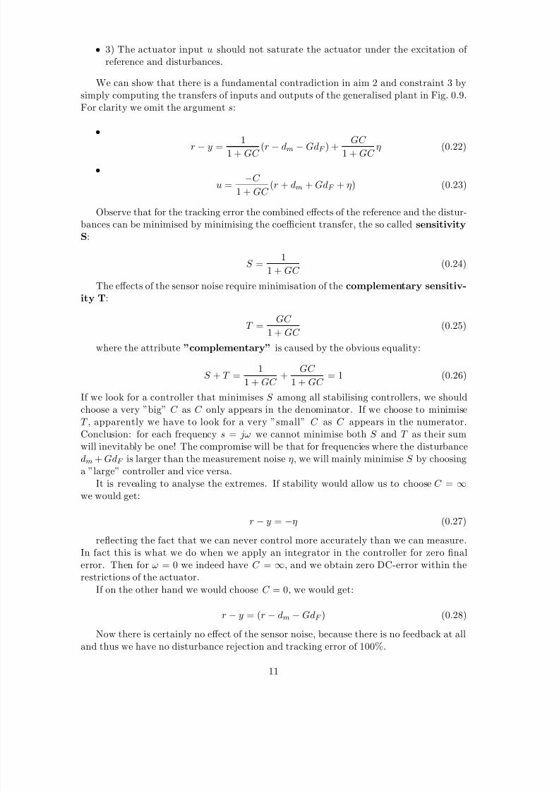
and take controller gain K such that we obtain equal real and imaginary parts for theclosed loop poles as shown in Fig. 0.10.

−20 −15 −10 −5 0 5 10 15 20−20

−15

−10

−5

0

5

10

15

20

Real Axis

I m a g A x i s

Figure 0.10: Rootlocus for PI-controlled nonminimumphase plant.

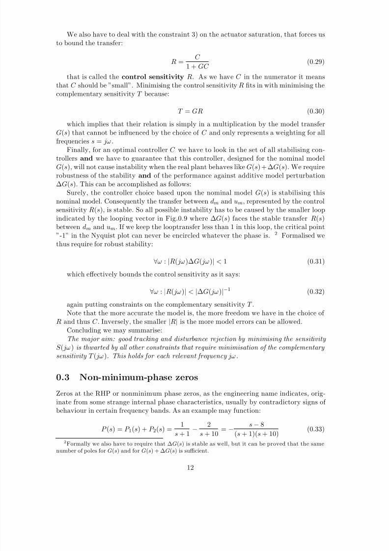
which leads to K = 3. In Fig. 0.11 the step response and the bode plot for the closedloop system is showed.

Time (sec.)

A m p l i t u d e

Step Response

0 0.5 1 1.5−1

−0.5

0

0.5

1

1.5From: U(1)

T o : Y ( 1 )

PC/s(PC+1)

P1C/s(P1C+1)

P2C/s(P2C+1)

10−1

100

101

102

10−2

10−1

100

101

PC/(PC+1)

P1C/(P1C+1)

P2C/(P2C+1)

Figure 0.11: Closed loop of nonminimum phase plant and its components.

Also the results for the same controller applied to the one component P 1(s) = 1/(s + 1)

13



or the other component P 2(s) = −2/(s + 10) is shown. The bodeplot shows a total gainenclosed by the two separate components and the component −2/(s + 10) is even morebroadbanded. Alas, if we would have only this component, the chosen controller wouldmake the plant unstable as seen in the step response. For the higher frequencies the phaseof the controller is incorrect. For the lower frequencies ω(0, 3.5) the phase of the controlleris appropriate and the plant is well controlled. The effect of the higher frequencies is stillseen at the initial time of the response where the direction (sign) is wrong.

As a consequence we cannot aim at a broader, low pass frequency band for trackingthan, as a rule of the thumb, ω(0, |z|/2).If, on the other hand, we would like to obtain a good tracking for a band ω(2|z|, 100|z|)

the controller can indeed well be chosen to control the component −2/(s + 10), while nowthe other component 1/(s + 1) is the nasty one. In a band ω(|z|/2, 2|z|) we can nevertrack well, because the opposite effects of both components of the plant are apparent intheir full extent.

If we have more RHP-zeros zi, we have as many forbidden tracking bands ω(|zi|/2, 2∗|zi|). Even zeros at infinity play a role as explained in the next section.

0.4 Bode integral.

For strictly proper plants combined with strictly proper controllers we will have zerosat infinity. It is irrelevant whether infinity is in the RHP. Zeros at infinity should betreated like all RHP-zeros, simply because they cannot be compensated by poles. Becausein practice each system is strictly proper, we have that the combination of plant andcontroller L(s) = P (s)C (s) has at least a pole zero excess (np−nz) of two. Consequentlywe have:

lims→∞ |S | = lim

s→∞ |1

1 + L(s)| = 1 (0.35)

which implies that inevitably for higher frequencies the system cannot track and wehave 100% tracking error and 100% disturbance.

Any tracking band will necessarily be bounded. However, how can we see the influ-ence of zeros at infinity at a finite band? Here the Bode Sensitivity Integral gives us animpression (the proof can be found in e.g. Doyle [1]). If the pole zero excess is at least 2and we have no RHP poles, the following holds:

∞0 ln |S ( jω)|dω = 0

The explanation can best be done with an example:

L(s) = P (s)C (s) =K

s(s + 100) (0.36)

so that the sensitivity in closed loop will be:

S =s(s + 100)

s2 + 100s + K (0.37)

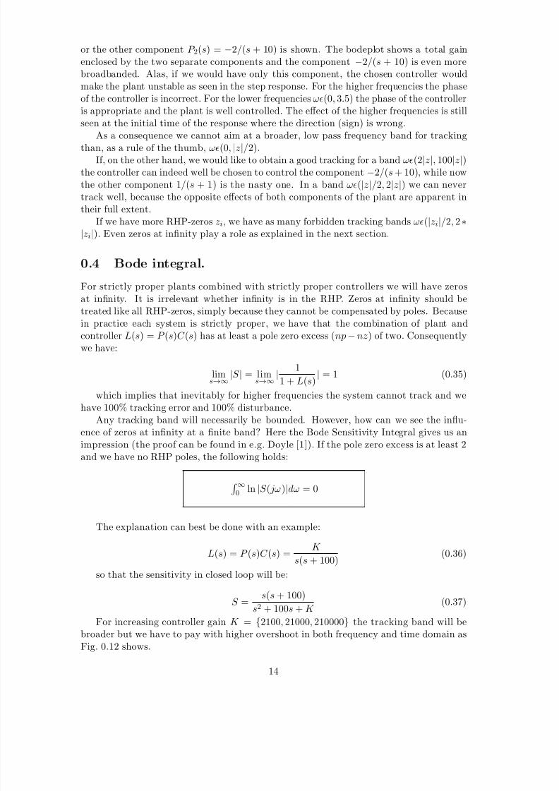
For increasing controller gain K = {2100, 21000, 210000} the tracking band will bebroader but we have to pay with higher overshoot in both frequency and time domain asFig. 0.12 shows.

14



10−1

100

101

102

103

104

10−5

10−4

10−3

10−2

10−1

100

101

K=2100

K=21000

K=210000

Figure 0.12: Sensitivity for looptransfer with pole zero excess

≤2 and no RHP-poles.

The Bode rule states that the area of |S ( jω)| under 0dB equals the area

above it.

Note that we have as usual a horizontal logarithmic scale for ω in Fig. 0.12 whichvisually disrupts the concepts of equal areas. Nevertheless the message is clear: the lesstracking error and disturbance we want to obtain over a broader band, the more we haveto pay for this by a more than 100% tracking error and disturbance multiplication outsidethis band.

0.5 RHP-poles.

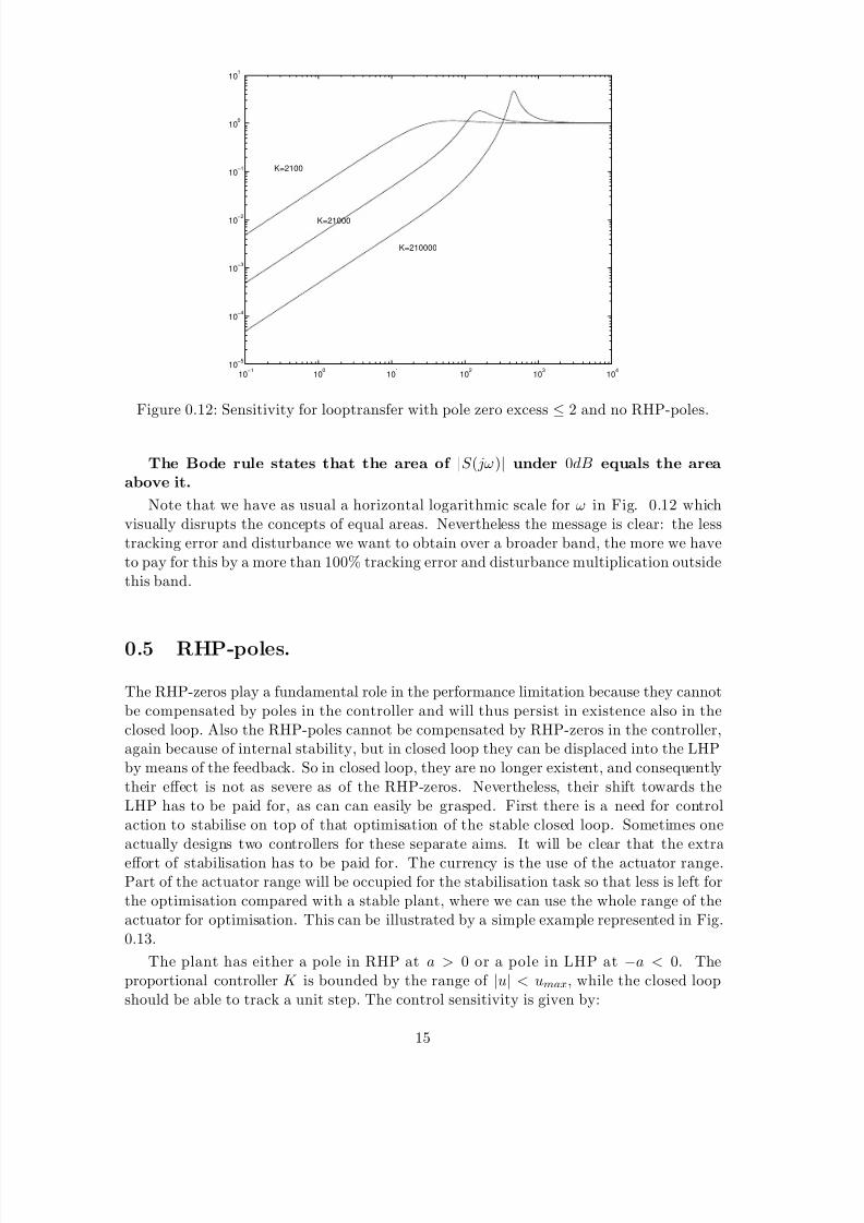
The RHP-zeros play a fundamental role in the performance limitation because they cannotbe compensated by poles in the controller and will thus persist in existence also in theclosed loop. Also the RHP-poles cannot be compensated by RHP-zeros in the controller,again because of internal stability, but in closed loop they can be displaced into the LHPby means of the feedback. So in closed loop, they are no longer existent, and consequentlytheir effect is not as severe as of the RHP-zeros. Nevertheless, their shift towards theLHP has to be paid for, as can can easily be grasped. First there is a need for controlaction to stabilise on top of that optimisation of the stable closed loop. Sometimes oneactually designs two controllers for these separate aims. It will be clear that the extra

effort of stabilisation has to be paid for. The currency is the use of the actuator range.Part of the actuator range will be occupied for the stabilisation task so that less is left forthe optimisation compared with a stable plant, where we can use the whole range of theactuator for optimisation. This can be illustrated by a simple example represented in Fig.0.13.

The plant has either a pole in RHP at a > 0 or a pole in LHP at −a < 0. Theproportional controller K is bounded by the range of |u| < umax, while the closed loopshould be able to track a unit step. The control sensitivity is given by:

15



K 1

s± a- - - -

?

6

r u+

−

Figure 0.13: Example for stabilisation effort.

R =u

r=

K

1 + K s±a

=K (s± a)

s ± a + K (0.38)

For stability we certainly need K > a. The maximum |u| for a unit step occurs att = 0 so:

maxt

(u) = u(0) = lims→∞R(s) = K = umax (0.39)

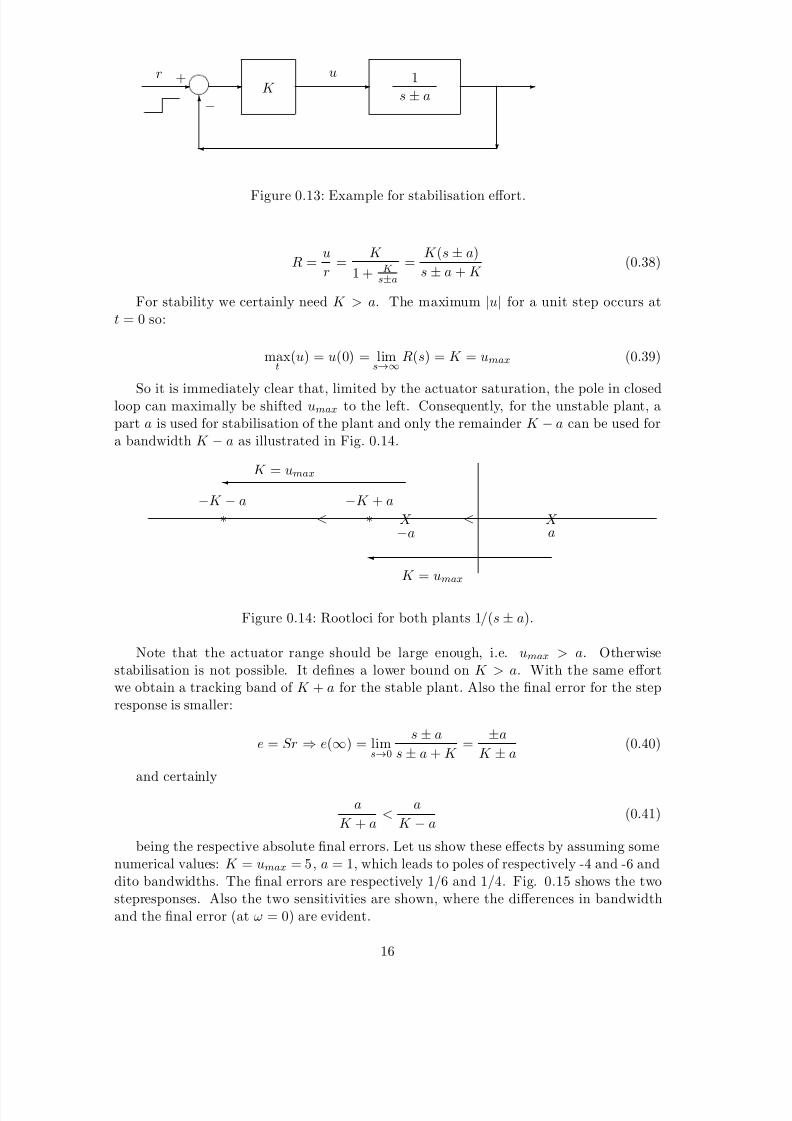
So it is immediately clear that, limited by the actuator saturation, the pole in closedloop can maximally be shifted umax to the left. Consequently, for the unstable plant, apart a is used for stabilisation of the plant and only the remainder K − a can be used fora bandwidth K − a as illustrated in Fig. 0.14.

X X a−a

∗∗

K = umax

K = umax

<<−K − a −K + a

Figure 0.14: Rootloci for both plants 1/(s± a).

Note that the actuator range should be large enough, i.e. umax > a. Otherwisestabilisation is not possible. It defines a lower bound on K > a. With the same effortwe obtain a tracking band of K + a for the stable plant. Also the final error for the stepresponse is smaller:

e = Sr ⇒ e(∞) = lims→0

s ± a

s± a + K =

±a

K ± a(0.40)

and certainly

a

K + a<

a

K − a(0.41)

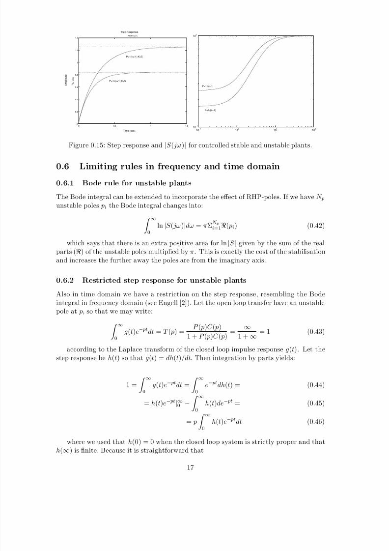
being the respective absolute final errors. Let us show these effects by assuming somenumerical values: K = umax = 5, a = 1, which leads to poles of respectively -4 and -6 anddito bandwidths. The final errors are respectively 1/6 and 1/4. Fig. 0.15 shows the twostepresponses. Also the two sensitivities are shown, where the differences in bandwidthand the final error (at ω = 0) are evident.

16



Time (sec.)

A m p l i t u d e

Step Response

0 0.5 1 1.50

0.2

0.4

0.6

0.8

1

1.2

1.4From: U(1)

T o : Y ( 1 )

P=1/(s+1) K=5

P=1/(s−1) K=5

10−1

100

101

102

10−1

100

P=1/(s−1)

P=1/(s+1)

Figure 0.15: Step response and |S ( jω)| for controlled stable and unstable plants.

0.6 Limiting rules in frequency and time domain

0.6.1 Bode rule for unstable plants

The Bode integral can be extended to incorporate the effect of RHP-poles. If we have N punstable poles pi the Bode integral changes into:

∞0

ln |S ( jω)|dω = πΣN pi=1( pi) (0.42)

which says that there is an extra positive area for ln |S | given by the sum of the realparts () of the unstable poles multiplied by π. This is exactly the cost of the stabilisationand increases the further away the poles are from the imaginary axis.

0.6.2 Restricted step response for unstable plants

Also in time domain we have a restriction on the step response, resembling the Bodeintegral in frequency domain (see Engell [2]). Let the open loop transfer have an unstablepole at p, so that we may write:

∞0

g(t)e− ptdt = T ( p) =P ( p)C ( p)

1 + P ( p)C ( p)=

∞1 + ∞ = 1 (0.43)

according to the Laplace transform of the closed loop impulse response g(t). Let thestep response be h(t) so that g(t) = dh(t)/dt. Then integration by parts yields:

1 = ∞0 g(t)e−

pt

dt = ∞0 e−

pt

dh(t) = (0.44)

= h(t)e− pt|∞0 − ∞0

h(t)de− pt = (0.45)

= p

∞0

h(t)e− ptdt (0.46)

where we used that h(0) = 0 when the closed loop system is strictly proper and thath(∞) is finite. Because it is straightforward that

17



∞0

e− ptdt = −1

p

∞0

de− pt = −e− pt

p|∞0 =

1

p(0.47)

the combination yields the restrictive time integral:

∞0 {1− h(t)}e− ptdt = 0

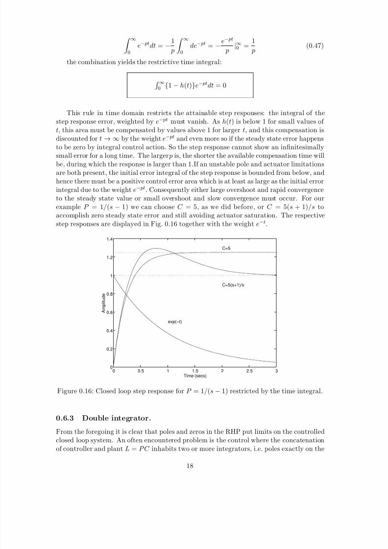
This rule in time domain restricts the attainable step responses: the integral of thestep response error, weighted by e− pt must vanish. As h(t) is below 1 for small values of t, this area must be compensated by values above 1 for larger t, and this compensation isdiscounted for t →∞ by the weight e− pt and even more so if the steady state error happensto be zero by integral control action. So the step response cannot show an infinitesimallysmall error for a long time. The larger p is, the shorter the available compensation time willbe, during which the response is larger than 1.If an unstable pole and actuator limitationsare both present, the initial error integral of the step response is bounded from below, andhence there must be a positive control error area which is at least as large as the initial error

integral due to the weight e− pt

. Consequently either large overshoot and rapid convergenceto the steady state value or small overshoot and slow convergence must occur. For ourexample P = 1/(s − 1) we can choose C = 5, as we did before, or C = 5(s + 1)/s toaccomplish zero steady state error and still avoiding actuator saturation. The respectivestep responses are displayed in Fig. 0.16 together with the weight e−t.

0 0.5 1 1.5 2 2.5 30

0.2

0.4

0.6

0.8

1

1.2

1.4

Time (secs)

A m p l i t u d e

exp(−t)

C=5(s+1)/s

C=5

Figure 0.16: Closed loop step response for P = 1/(s − 1) restricted by the time integral.

0.6.3 Double integrator.

From the foregoing it is clear that poles and zeros in the RHP put limits on the controlledclosed loop system. An often encountered problem is the control where the concatenationof controller and plant L = P C inhabits two or more integrators, i.e. poles exactly on the

18



stability border in s = 0. E.g. the plant has one integrator (servosystem) and in orderto obtain a zero DC-error for disturbing inputs (force), one is obliged to incorporate anintegrator in the controller as well. For that situation we have a nasty limiting rule instepresponse similar to the RHP-poles effect:

∞0 {1− h(t)}dt = 0

The proof is as follows (in the same notation as for the RHP-pole rule):Simple Laplace transform states:

∞0{1− h(t)}e−stdt =

1

s− 1

sT (s) (0.48)

furthermore:

lims→0

1− T (s)

s= lim

s→0

1− PC 1+PC

s= lim

s→0

1

s + sP C = 0 (0.49)

because

lims→0

sP (s)C (s) = ∞ (0.50)

as PC have at least two integrators. QED

19



0.7 Design example

The aim of this chapter is to synthesize a classic controller for a rocket model with per-turbations. The program files which will be used can be obtained from the public foldersof this course.

0.7.1 Plant definition

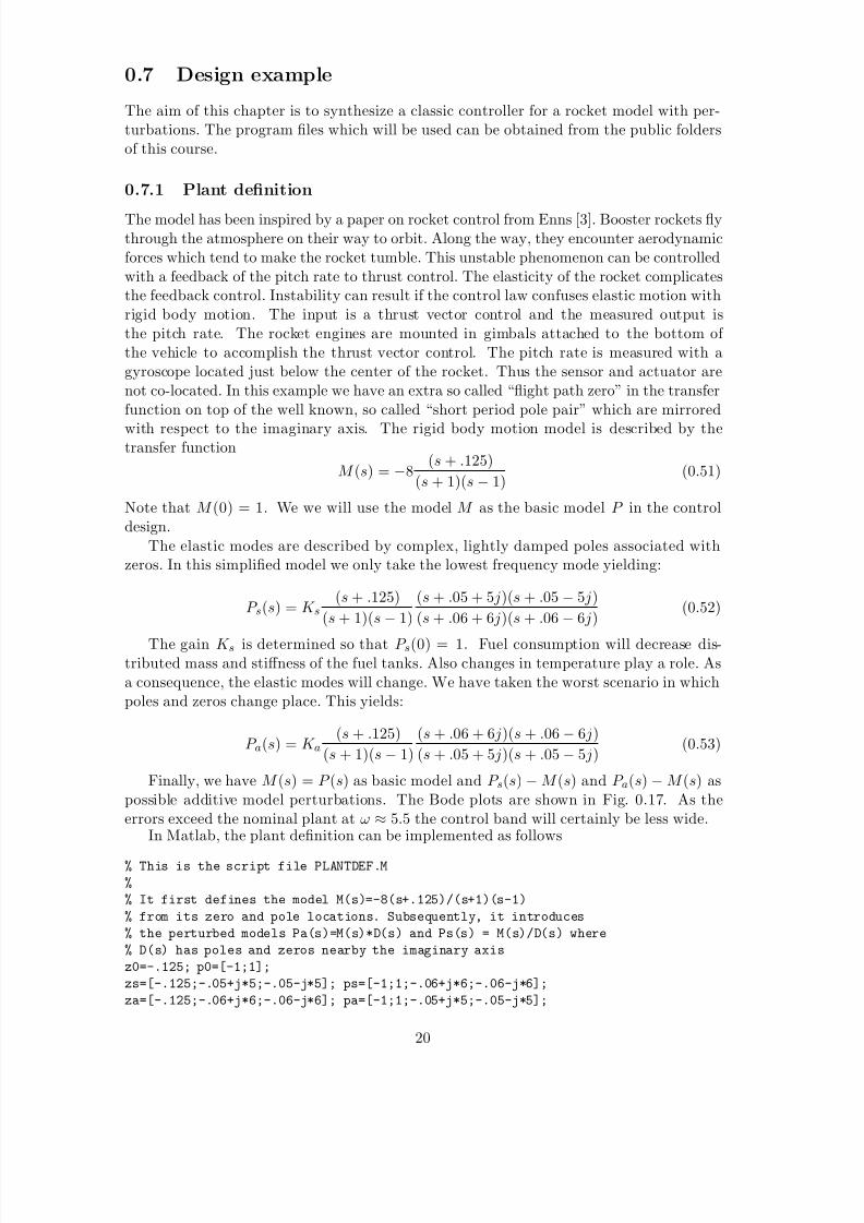
The model has been inspired by a paper on rocket control from Enns [3]. Booster rockets flythrough the atmosphere on their way to orbit. Along the way, they encounter aerodynamicforces which tend to make the rocket tumble. This unstable phenomenon can be controlledwith a feedback of the pitch rate to thrust control. The elasticity of the rocket complicatesthe feedback control. Instability can result if the control law confuses elastic motion withrigid body motion. The input is a thrust vector control and the measured output isthe pitch rate. The rocket engines are mounted in gimbals attached to the bottom of the vehicle to accomplish the thrust vector control. The pitch rate is measured with agyroscope located just below the center of the rocket. Thus the sensor and actuator arenot co-located. In this example we have an extra so called “flight path zero” in the transferfunction on top of the well known, so called “short period pole pair” which are mirrored

with respect to the imaginary axis. The rigid body motion model is described by thetransfer function

M (s) = −8(s + .125)

(s + 1)(s − 1)(0.51)

Note that M (0) = 1. We we will use the model M as the basic model P in the controldesign.

The elastic modes are described by complex, lightly damped poles associated withzeros. In this simplified model we only take the lowest frequency mode yielding:

P s(s) = K s(s + .125)

(s + 1)(s− 1)

(s + .05 + 5 j)(s + .05 − 5 j)

(s + .06 + 6 j)(s + .06 − 6 j)(0.52)

The gain K s is determined so that P s(0) = 1. Fuel consumption will decrease dis-tributed mass and stiffness of the fuel tanks. Also changes in temperature play a role. Asa consequence, the elastic modes will change. We have taken the worst scenario in whichpoles and zeros change place. This yields:

P a(s) = K a(s + .125)

(s + 1)(s− 1)

(s + .06 + 6 j)(s + .06− 6 j)

(s + .05 + 5 j)(s + .05− 5 j)(0.53)

Finally, we have M (s) = P (s) as basic model and P s(s) − M (s) and P a(s) − M (s) aspossible additive model perturbations. The Bode plots are shown in Fig. 0.17. As theerrors exceed the nominal plant at ω ≈ 5.5 the control band will certainly be less wide.

In Matlab, the plant definition can be implemented as follows

% This is the script file PLANTDEF.M

%

% It first defines the model M(s)=-8(s+.125)/(s+1)(s-1)

% from its zero and pole locations. Subsequently, it introduces

% the perturbed models Pa(s)=M(s)*D(s) and Ps(s) = M(s)/D(s) where

% D(s) has poles and zeros nearby the imaginary axis

z0=-.125; p0=[-1;1];

zs=[-.125;-.05+j*5;-.05-j*5]; ps=[-1;1;-.06+j*6;-.06-j*6];

za=[-.125;-.06+j*6;-.06-j*6]; pa=[-1;1;-.05+j*5;-.05-j*5];

20



10−3

10−2

10−1

100

101

102

10−7

10−6

10−5

10−4

10

−3

10−2

10−1

100

101

102

|M|,|M−Ps|,|M−Pa|

The plant and its perturbations

Figure 0.17: Nominal plant and additive perturbations.

[numm,denm]=zp2tf(z0,p0,1);

[nums,dens]=zp2tf(zs,ps,1);[numa,dena]=zp2tf(za,pa,1);

% adjust the gains:

km=polyval(denm,0)/polyval(numm,0);

ks=polyval(dens,0)/polyval(nums,0);

ka=polyval(dena,0)/polyval(numa,0);

numm=numm*km;nums=nums*ks;numa=numa*ka;

% Define error models M-Pa and M-Ps

[dnuma,ddena]=parallel(numa,dena,-numm,denm);

[dnums,ddens]=parallel(nums,dens,-numm,denm);

% Plot the bode diagram of model and its (additive) errors

w=logspace(-3,2,3000);

magm=bode(numm,denm,w); mags=bode(dnums,ddens,w);

dmaga=bode(dnuma,ddena,w);

dmags=bode(dnums,ddens,w);

loglog(w,magm,w,dmags,w,dmaga);

title(’|M|,|M-Ps|,|M-Pa|’);

xlabel(’The plant and its perturbations’);

0.7.2 Classic control

The plant is a simple SISO-system, so we should be able to design a controller with classictools.

For the controlled system we wish to obtain a zero steady state, i.e., integral action.The bandwidth is bounded by the actuator and by the elastic mode at approximately 5.5rad/s, as we require robust stability and robust performance for the elastic mode models.Some trial and error with a simple low order controller, leads soon to a controller of theform

C (s) = −1

2

(s + 1)

s(s + 2)(0.54)

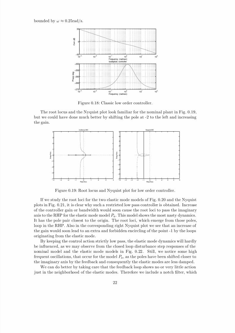
In the bode plot of this controller in Fig. 0.18, we observe that the control band is

21



bounded by ω ≈ 0.25rad/s.

10−3

10−2

10−1

100

101

102

−50

0

50

Frequency (rad/sec)

G a i n d B

10−3

10−2

10−1

100

101

102

−270

−265

−260

−255

−250

Frequency (rad/sec)

P h a s e d e g

bodeplots controller

Figure 0.18: Classic low order controller.

The root locus and the Nyquist plot look familiar for the nominal plant in Fig. 0.19,

but we could have done much better by shifting the pole at -2 to the left and increasingthe gain.

−4 −3 −2 −1 0 1 2 3 4−4

−3

−2

−1

0

1

2

3

4

Real Axis

I m a g A x i s

rootlocus MC

−5 −4 −3 −2 −1 0 1 2 3 4 5−5

−4

−3

−2

−1

0

1

2

3

4

5

Real Axis

I m a g A x i s

Nyquist MC

Figure 0.19: Root locus and Nyquist plot for low order controller.

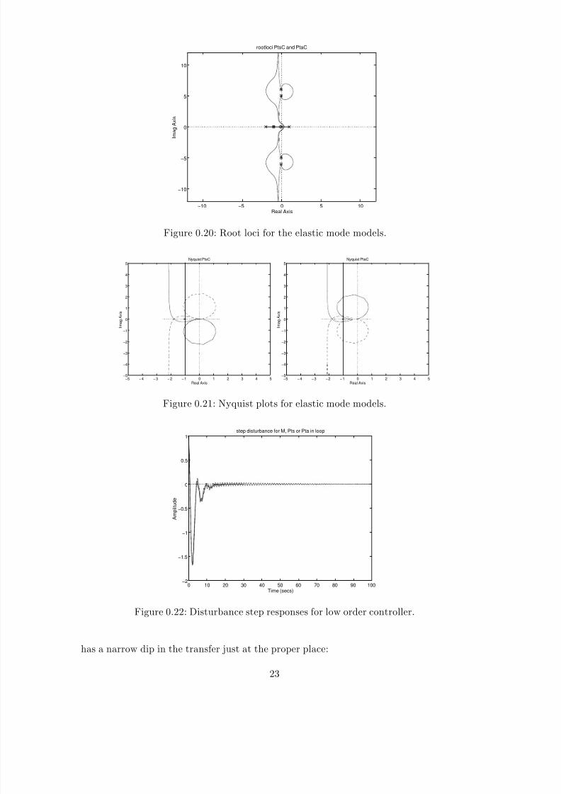
If we study the root loci for the two elastic mode models of Fig. 0.20 and the Nyquistplots in Fig. 0.21, it is clear why such a restricted low pass controller is obtained. Increaseof the controller gain or bandwidth would soon cause the root loci to pass the imaginaryaxis to the RHP for the elastic mode model P a. This model shows the most nasty dynamics.It has the pole pair closest to the origin. The root loci, which emerge from those poles,loop in the RHP. Also in the corresponding right Nyquist plot we see that an increase of the gain would soon lead to an extra and forbidden encircling of the point -1 by the loopsoriginating from the elastic mode.

By keeping the control action strictly low pass, the elastic mode dynamics will hardlybe influenced, as we may observe from the closed loop disturbance step responses of thenominal model and the elastic mode models in Fig. 0.22. Still, we notice some highfrequent oscillations, that occur for the model P a, as the poles have been shifted closer tothe imaginary axis by the feedback and consequently the elastic modes are less damped.

We can do better by taking care that the feedback loop shows no or very little action just in the neighborhood of the elastic modes. Therefore we include a notch filter, which

22





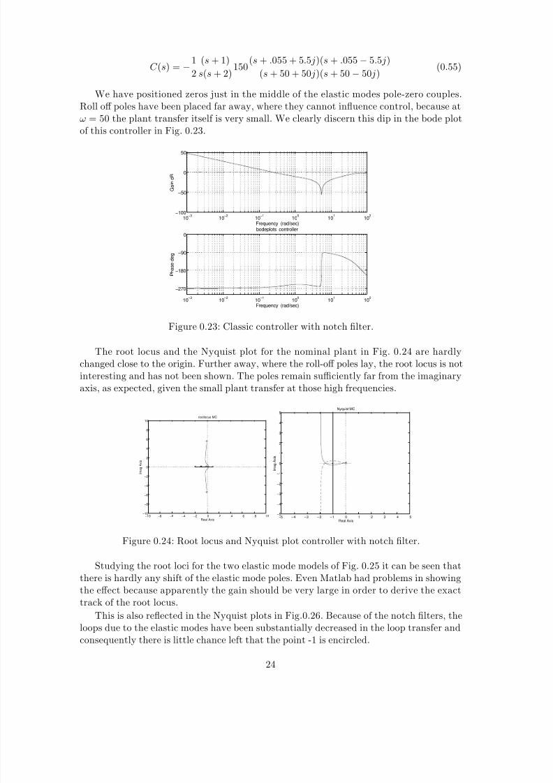
C (s) = −1

2

(s + 1)

s(s + 2)150

(s + .055 + 5.5 j)(s + .055− 5.5 j)

(s + 50 + 50 j)(s + 50 − 50 j)(0.55)

We have positioned zeros just in the middle of the elastic modes pole-zero couples.Roll off poles have been placed far away, where they cannot influence control, because atω = 50 the plant transfer itself is very small. We clearly discern this dip in the bode plotof this controller in Fig. 0.23.

10−3

10−2

10−1

100

101

102

−100

−50

0

50

Frequency (rad/sec)

G a i n d B

10−3

10−2

10−1

100

101

102

−90

−180

−270

0

Frequency (rad/sec)

P

h a s e d e g

bodeplots controller

Figure 0.23: Classic controller with notch filter.

The root locus and the Nyquist plot for the nominal plant in Fig. 0.24 are hardlychanged close to the origin. Further away, where the roll-off poles lay, the root locus is notinteresting and has not been shown. The poles remain sufficiently far from the imaginaryaxis, as expected, given the small plant transfer at those high frequencies.

−10 −8 −6 −4 −2 0 2 4 6 8 10−10

−8

−6

−4

−2

0

2

4

6

8

10

Real Axis

I m a g A x i s

rootlocus MC

−5 −4 −3 −2 −1 0 1 2 3 4 5−5

−4

−3

−2

−1

0

1

2

3

4

5

Real Axis

I m a g A x i s

Nyquist MC

Figure 0.24: Root locus and Nyquist plot controller with notch filter.

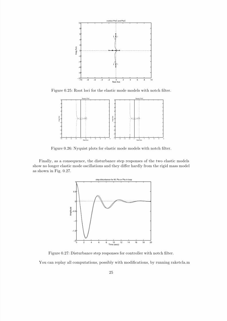
Studying the root loci for the two elastic mode models of Fig. 0.25 it can be seen thatthere is hardly any shift of the elastic mode poles. Even Matlab had problems in showingthe effect because apparently the gain should be very large in order to derive the exacttrack of the root locus.

This is also reflected in the Nyquist plots in Fig.0.26. Because of the notch filters, theloops due to the elastic modes have been substantially decreased in the loop transfer andconsequently there is little chance left that the point -1 is encircled.

24



−10 −8 −6 −4 −2 0 2 4 6 8 10−10

−8

−6

−4

−2

0

2

4

6

8

10

Real Axis

I m a g A x i s

rootloci PtsC and PtaC

Figure 0.25: Root loci for the elastic mode models with notch filter.

−5 −4 −3 −2 −1 0 1 2 3 4 5−5

−4

−3

−2

−1

0

1

2

3

4

5

Real Axis

I m a g A x i s

Nyquist PtsC

−5 −4 −3 −2 −1 0 1 2 3 4 5−5

−4

−3

−2

−1

0

1

2

3

4

5

Real Axis

I m a g A x i s

Nyquist PtaC

Figure 0.26: Nyquist plots for elastic mode models with notch filter.

Finally, as a consequence, the disturbance step responses of the two elastic modelsshow no longer elastic mode oscillations and they differ hardly from the rigid mass modelas shown in Fig. 0.27.

0 2 4 6 8 10 12 14 16 18 20−2

−1.5

−1

−0.5

0

0.5

1

Time (secs)

A m p l i t u d e

step disturbance for M, Pts or Pta in loop

Figure 0.27: Disturbance step responses for controller with notch filter.

You can replay all computations, possibly with modifications, by running raketcla.m

25



as listed below:

% This is the script file RAKETCLA.M

%

% In this script file we synthesize controllers

% for the plant (defined in plantdef) using classical

% design techniques. It is assumed that you ran

% *plantdef* before invoking this script.

%% First try the classic control law: C(s)=-.5(s+1)/s(s+2)

numc=-[.5 .5]; denc=[1 2 0];

bode(numc,denc,w); title(’bodeplots controller’);

pause;

numl=conv(numc,numm); denl=conv(denc,denm);

rlocus(numl,denl); title(’rootlocus MC’);

pause;

nyquist(numl,denl,w);

set(figure(1),’currentaxes’,get(gcr,’plotaxes’))

axis([-5,5,-5,5]); title(’Nyquist MC’);

pause;

[numls,denls]=series(numc,denc,nums,dens);[numla,denla]=series(numc,denc,numa,dena);

rlocus(numls,denls); hold;

rlocus(numla,denla); title(’rootloci PtsC and PtaC’);

pause; hold off;

nyquist(numls,denls,w);


axis([-5,5,-5,5]); title(’Nyquist PtsC’);

pause;

nyquist(numla,denla,w);


axis([-5,5,-5,5]); title(’Nyquist PtaC’);

pause;

[numcl,dencl]=feedback(1,1,numl,denl,-1);[numcls,dencls]=feedback(1,1,numls,denls,-1);

[numcla,dencla]=feedback(1,1,numla,denla,-1);

step(numcl,dencl); hold;

step(numcls,dencls); step(numcla,dencla);

title(’step disturbance for M, Pts or Pta in loop’);

pause; hold off;

% Improved classic controller C(s)=-[.5(s+1)/s(s+2)]*

% 150(s+.055+j*5.5)(s+.055-j*5.5)/(s+50-j*50)(s+50-j*50)

numc=conv(-[.5 .5],[1 .1 30.2525]*150);

denc=conv([1 2 0],[1 100 5000]);

bode(numc,denc,w); title(’bodeplots controller’);

pause;

numl=conv(numc,numm); denl=conv(denc,denm);

rlocus(numl,denl);

axis([-10,10,-10,10]); title(’rootlocus MC’);

pause;

nyquist(numl,denl,w);


axis([-5,5,-5,5]); title(’Nyquist MC’);

26



pause;

[numls,denls]=series(numc,denc,nums,dens);

[numla,denla]=series(numc,denc,numa,dena);

rlocus(numls,denls); hold; rlocus(numla,denla);

axis([-10,10,-10,10]); title(’rootloci PtsC and PtaC’);

pause; hold off;

nyquist(numls,denls,w);


axis([-5,5,-5,5]); title(’Nyquist PtsC’);pause;

nyquist(numla,denla,w);


axis([-5,5,-5,5]); title(’Nyquist PtaC’);

pause;

[numcl,dencl]=feedback(1,1,numl,denl,-1);

[numcls,dencls]=feedback(1,1,numls,denls,-1);

[numcla,dencla]=feedback(1,1,numla,denla,-1);

step(numcl,dencl);

hold;

step(numcls,dencls);step(numcla,dencla);

title(’step disturbance for M, Pts or Pta in loop’);

pause; hold off;

27



28



Bibliography

[1] J. Doyle, B. Francis, A. Tannenbaum, “Feedback Control Theory,” McMillan Publish-ing Co., 1990.

[2] S. Engell, “Design of Robust Control Systems with Time-Domain Specifications”, Con-trol Eng. Practice, Vol.3, No.3, pp.365-372, 1995.

[3] D.F. Enns, “Structured Singular Value Synthesis Design Example: Rocket Stabilisa-tion”, American Control Conf., Vol.3, pp.2514-2520, 1990.

Documents

Limits of Feedback and RHP