Limited Arbitrage in Equity Markets

MARK MITCHELL, TODD PULVINO, and ERIK STAFFORD*

ABSTRACT

We examine 82 situations where the market value of a company is less than itssubsidiary. These situations imply arbitrage opportunities, providing an idealsetting to study the risks and market frictions that prevent arbitrageurs fromimmediately forcing prices to fundamental values. For 30 percent of the sample,the link between the parent and its subsidiary is severed before the relative valuediscrepancy is corrected. Furthermore, returns to a specialized arbitrageur wouldbe 50 percent larger if the path to convergence was smooth rather than asobserved. Uncertainty about the distribution of returns and characteristics of therisks limits arbitrage.

* Mitchell and Stafford are at Harvard University, and Pulvino is at Northwestern University.

We thank Brad Cornell, Kent Daniel, Mihir Desai, Rick Green, Ravi Jagannathan, Owen

Lamont, André Perold, Mitch Petersen, Julio Rotemberg, Rick Ruback, Tuomo Vuolteenaho, an

anonymous referee, and seminar participants at the Federal Reserve Bank of New York, Harvard

Business School, Ohio State University, and the 2001 Spring NBER Asset Pricing Program

Meetings for helpful comments. We also thank Asma Qureshi for research assistance,

Ameritrade Holding Corporation for short-rebate data, and especially Ken French for insightful

comments and discussions. Harvard Business School’s Division of Research provided research

support.

1

This paper examines impediments to arbitrage in equity markets using a sample of 82 situations

between 1985 and 2000, where the market value of a company is less than that of its ownership

stake in a publicly-traded subsidiary. These situations suggest clear arbitrage opportunities, yet,

they often persist, and therefore provide an interesting setting in which to study the risks and

market frictions that prevent arbitrageurs from quickly forcing prices to fundamental values.

Arbitrage is one of the central tenets of financial economics, enforcing the law of one

price and keeping markets efficient. In its purest form, arbitrage requires no capital and is

riskfree (see Dybvig and Ross (1992)). By simultaneously selling and purchasing identical

securities at favorably different prices, the arbitrageur captures an immediate payoff with no up-

front capital. Unfortunately, pure arbitrage exists only in perfect capital markets. In the real

world, imperfect information and market frictions make what is referred to as “arbitrage” both

capital intensive and risky.

Imperfect information and market frictions can impede arbitrage in two different ways.

First, when there is uncertainty over the economic nature of an apparent mispricing and it is at

least somewhat costly to learn about it, arbitrageurs may be reluctant to incur the potentially

large fixed costs of entering the business of exploiting the arbitrage opportunity (Merton (1987)).

Uncertainty over the distribution of arbitrage returns, especially over the mean, will deter

arbitrage activity until would-be arbitrageurs learn enough about the distribution to determine

that the expected payoff is large enough to cover the fixed costs of setting up shop. Even with

active arbitrageurs, opportunities may persist while the arbitrageurs learn how to best exploit

them.

Second, once the fixed costs of implementing the arbitrage strategy are borne, imperfect

information and market frictions often encourage specialization. Specialization limits the degree

of diversification in the arbitrageur’s portfolio and causes him to bear idiosyncratic risks for

which he must be rewarded. For example, if there is a purely random chance that prices will not

converge to fundamental value, a highly specialized arbitrageur who cannot diversify away this

risk will invest less than one who can. Furthermore, even if prices eventually converge to

2

fundamental values, the path of convergence may be long and bumpy. While waiting for the

prices of the mispriced securities to converge, they may temporarily diverge. If the arbitrageur

does not have access to additional capital when the security prices diverge, he may be forced to

prematurely unwind the position and incur a loss (DeLong, et al. (1990), Shleifer and Summers

(1990), and Shleifer and Vishny (1997)). The prospect of incurring this loss will further limit the

amount that a specialized arbitrageur is willing to invest.

To empirically address the limits of arbitrage in equity markets, we construct a sample of

situations where a firm’s market value is less than the value of its ownership stake in a publicly-

traded subsidiary.1 These situations are commonly referred to as “negative-stub-values” and can

arise following equity carve outs of subsidiaries or from the partial acquisition of a publicly-

traded firm. We track each parent/subsidiary pair until an event occurs that eliminates the link

between the two entities or until the mispricing disappears. Favorable outcomes include prices

adjusting to eliminate the relative value discrepancy and distributions of the subsidiary shares to

the parent firm’s shareholders, while unfavorable terminations tend to be associated with

acquisitions of the subsidiary and performance-related delistings of the parent. We attempt to

control for the role that market frictions play in explaining the persistence of negative-stub-

values by incorporating estimates of market frictions such as brokerage commissions, short-

rebates, and capital requirements into the analysis. The empirical results provide considerable

support for the argument that there are costs that limit arbitrage in equity markets.2

We show that negative-stub-values are not riskfree arbitrage opportunities. The link

between parent and subsidiary firms disappears without convergence of the arbitrage spread 30

percent of the time. This happens when there is a corporate event that permanently alters the

relative mispricing in a manner that is detrimental to the arbitrageur’s profits. For example, in

some negative-stub-value situations in our sample, the parent firm goes bankrupt after using its

subsidiary stake as collateral to issue debt. As a result, the link between the parent and

subsidiary firms’ market values is permanently severed without convergence of the arbitrage

spread.

3

We also find that there is substantial variability in the time to termination, even for

negative-stub-value investments that eventually converge. The average time between the initial

mispricing and a terminating event is 236 days, the median is 92 days, the minimum is one day,

and the maximum is 2,796 days. As a result of this uncertainty, even if convergence is

eventually achieved, the negative-stub-value investment often underperforms the riskfree rate,

thereby discouraging investments by arbitrageurs who are uncertain of the time to convergence

and unable to close the arbitrage spread on their own.

The analysis indicates that annual returns to a specialized arbitrageur would be roughly

50 percent higher if the path to termination was smooth rather than the observed bumpy path.

We estimate that when an investor posts sufficient collateral to insure against the bumpiness of

the path to termination, returns are just barely larger than the riskfree rate. However, the effect

of the volatile path can be substantially mitigated by combining negative-stub-value investments

with the market portfolio or with other “special situations” such as merger arbitrage. This

benefit of diversification, combined with the infrequent occurrence of negative-stub-value

situations, suggests that it is unlikely that an arbitrageur would focus solely on negative-stub-

values.

Finally, we document that the general uncertainty over the distribution of returns is a

significant contributor to the persistence of negative-stub-values. We find (1) that statistical

reliability of abnormal returns is fairly low at the end of our 16-year sample period, and therefore

unreliable near the beginning of the sample, (2) very unusual events cause extreme adverse

valuation changes 13 years into the sample time series, such that even a seasoned arbitrageur

would likely be caught off guard, and (3) statistically and economically large price movements

occur on the day that uncertainty over the outcome is resolved. For example, when parent

companies announce their intentions to distribute the subsidiaries’ shares to parent company

shareholders, or when they announce receipt of favorable IRS tax rulings regarding the

distribution of shares, the value of the arbitrageur’s position increases substantially over the three

days surrounding the announcement. Even in the lowest risk cases, where the parent has

4

previously announced its intention to distribute subsidiary shares, the value of the arbitrage

position increases 8.7 percent when the parent announces receipt of a favorable IRS ruling or

specifies a date for the distribution. Moreover, with no change in the availability of shares for

shorting, prices quickly adjust such that estimated stub-values are no longer negative once this

uncertainty is resolved.

This paper is organized as follows. Section I describes the data, Section II discusses the

measurement of investment returns and performance, Section III reports results relating to the

fundamental risk of negative-stub-value investments, Section IV reports results relating to the

financing risk of negative-stub-value investments, Section V interprets the results and discusses

arbitrage in imperfect capital markets, and Section VI concludes.

I. Data Description

A. Sample Selection Criteria

To be included in the sample, the parent’s stub assets must, at some time, have an implied

market value less than zero. Stub assets are defined as the market value of the parent’s equity

less any measurable net assets net of the parent’s unconsolidated liabilities.

[ ]sLiabilitieAssetsOtherStakeEquityStub MVMVMVMVV −−−= . (1)

We use two different methods to determine whether the stub assets have a negative value. The

first method, which we refer to as Rule 1, assumes that the market value of the parent’s non-

subsidiary assets is equal to the market value of its liabilities. Therefore, the stub-value is

negative whenever the market value of the parent’s equity stake in the subsidiary exceeds the

parent’s total market equity value:

0.1if 0:1# Rule

><EquityParent

StakeStub MV

MVV .(2)

Our second approach to identifying negative-stub-values is to assume that the difference

between the market value of the parent’s non-subsidiary assets (other assets) and the market

5

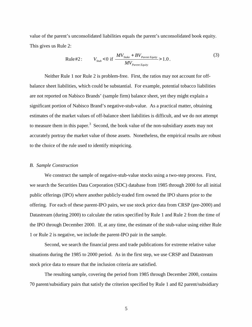
value of the parent’s unconsolidated liabilities equals the parent’s unconsolidated book equity.

This gives us Rule 2:

0.1if 0:2#Rule

>+

<EquityParent

EquityParentStakeStub MV

BVMVV .

(3)

Neither Rule 1 nor Rule 2 is problem-free. First, the ratios may not account for off-

balance sheet liabilities, which could be substantial. For example, potential tobacco liabilities

are not reported on Nabisco Brands’ (sample firm) balance sheet, yet they might explain a

significant portion of Nabisco Brand’s negative-stub-value. As a practical matter, obtaining

estimates of the market values of off-balance sheet liabilities is difficult, and we do not attempt

to measure them in this paper.3 Second, the book value of the non-subsidiary assets may not

accurately portray the market value of those assets. Nonetheless, the empirical results are robust

to the choice of the rule used to identify mispricing.

B. Sample Construction

We construct the sample of negative-stub-value stocks using a two-step process. First,

we search the Securities Data Corporation (SDC) database from 1985 through 2000 for all initial

public offerings (IPO) where another publicly-traded firm owned the IPO shares prior to the

offering. For each of these parent-IPO pairs, we use stock price data from CRSP (pre-2000) and

Datastream (during 2000) to calculate the ratios specified by Rule 1 and Rule 2 from the time of

the IPO through December 2000. If, at any time, the estimate of the stub-value using either Rule

1 or Rule 2 is negative, we include the parent-IPO pair in the sample.

Second, we search the financial press and trade publications for extreme relative value

situations during the 1985 to 2000 period. As in the first step, we use CRSP and Datastream

stock price data to ensure that the inclusion criteria are satisfied.

The resulting sample, covering the period from 1985 through December 2000, contains

70 parent/subsidiary pairs that satisfy the criterion specified by Rule 1 and 82 parent/subsidiary

6

pairs that satisfy the criterion specified by Rule 2. Table I provides an annual summary of the

negative-stub-value situations included in our sample by industry sector identified using Rule 1.

Panel A shows that the sample covers a range of sectors, with a relatively high concentration in

the technology sector during the latter part of the sample period. Panel B reports that many of

the subsidiaries in the latter part of the sample period are firms with an “Internet” focus.

[Insert Table I around here]

C. Shares Outstanding, Returns, and Short-Rebates

In order to estimate the stub-value in cross-holding situations, the number of parent

shares outstanding and the number of subsidiary shares held by the parent are needed. We

collect data on shares outstanding from quarterly company filings of financial reports.4 Because

estimates of arbitrage profits depend crucially on the numbers of shares outstanding at each point

in time, we identify exact dates at which shares outstanding change whenever the number of

shares indicated in quarterly reports change by at least 10 percent. Exact dates are determined by

searching the financial press for relevant news.

In addition to share price and share ownership data, accurately assessing the risks and

market frictions associated with negative-stub-value trades requires estimates of “short-rebates.”

Short-rebate refers to the rate paid to investors on the proceeds obtained from short selling a

stock. We obtained short-rebate data from Ameritrade Holding Corporation, a large online retail

broker. This short-rebate data covers the December 1998 through October 2000 time period.

The data represent the interest rates that other institutions (typically large Wall Street investment

banks) received from Ameritrade on the cash collateral that they posted to borrow Ameritrade’s

shares. Generally, the short-rebate is 25 to 50 basis points less than the federal funds rate.

However, the short-rebate is occasionally lower and can even be negative. Because we observe

short-rebates only for securities borrowed from Ameritrade, it is likely that our short-rebate

sample is biased toward stocks that are in high demand for shorting. Otherwise, the borrowing

institutions would take them directly from their own inventory and would not need to borrow

them from Ameritrade.

7

II. Measuring Investment Returns

In order to calculate returns and characterize risks associated with negative-stub-value

investments, we begin by specifying an investment strategy. Implementing this strategy requires

that the investor define the following four items: (1) the criterion by which the stub is judged to

be mispriced, (2) the buy threshold, (3) the sell threshold, and (4) the amount of financial

leverage used (the short position in the subsidiary’s shares makes it impossible to invest in a

negative-stub-value situation on an unlevered basis).

A. Investment Criteria and Thresholds

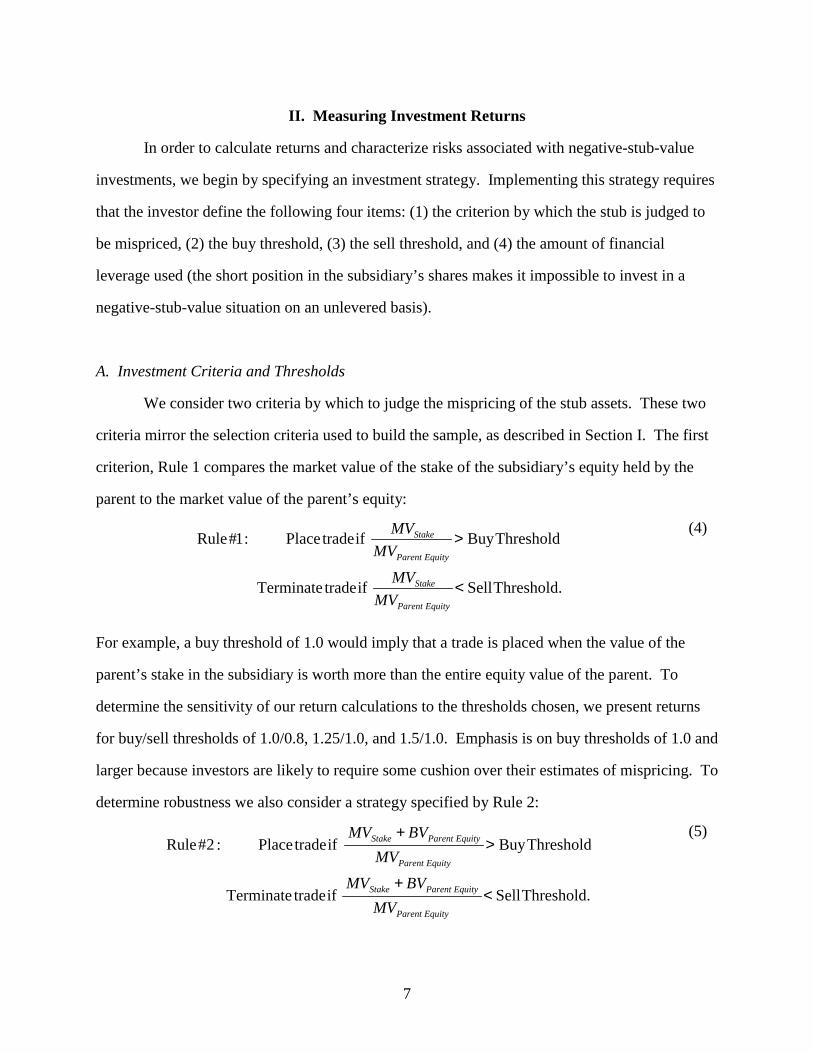
We consider two criteria by which to judge the mispricing of the stub assets. These two

criteria mirror the selection criteria used to build the sample, as described in Section I. The first

criterion, Rule 1 compares the market value of the stake of the subsidiary’s equity held by the

parent to the market value of the parent’s equity:

Threshold.Sell iftradeTerminate

ThresholdBuyiftradePlace:1#Rule

<

>

EquityParent

Stake

EquityParent

Stake

MVMV

MVMV (4)

For example, a buy threshold of 1.0 would imply that a trade is placed when the value of the

parent’s stake in the subsidiary is worth more than the entire equity value of the parent. To

determine the sensitivity of our return calculations to the thresholds chosen, we present returns

for buy/sell thresholds of 1.0/0.8, 1.25/1.0, and 1.5/1.0. Emphasis is on buy thresholds of 1.0 and

larger because investors are likely to require some cushion over their estimates of mispricing. To

determine robustness we also consider a strategy specified by Rule 2:

Threshold.Sell iftradeTerminate

ThresholdBuyiftradePlace:2#Rule

<+

>+

EquityParent

EquityParentStake

EquityParent

EquityParentStake

MVBVMV

MVBVMV (5)

8

B. Investment Capital and Financial Leverage

A final parameter that must be specified before returns can be calculated is the initial

investment capital. Although straightforward for portfolios that contain only long positions, the

appropriate denominator for calculating returns for a portfolio with both long and short positions

is less obvious. In a frictionless capital market, the object of interest would simply be a short

position in the subsidiary and a long position in the parent, which holds shares in the subsidiary.

The long position would be fully financed by the proceeds from the short position. This does not

work in real markets because the investor must post collateral for both long and short positions.

Furthermore, the investor does not receive full use of the proceeds from a short position.

Therefore, we calculate the return on the capital that is required to undertake the arbitrage trade.

For example, an investor wishing to buy one share of a parent stock trading at $26.25 and sell

short 0.7154 shares of a subsidiary stock with a price of $48.00 is required to contribute capital

of at least $30.29 (50 percent of both long and short position) to satisfy minimum initial capital

requirements imposed by the Federal Reserve Board. To calculate returns, the total payoff from

the long- and short-stock positions, as well as the net interest payments from any excess cash

minus margin borrowing is divided by the $30.29 equity capital base. In addition to posting the

required capital, investors may choose to allocate additional precautionary capital to lower the

leverage of the position. Because choosing the denominator in the return calculation requires

one to specify financial leverage, and since financial leverage has a direct effect on both the

return and the risk, we present results using three leverage levels.

We refer to the first leverage level as “textbook” leverage. Results calculated using

textbook leverage are based on two assumptions. The first assumption is based on Regulation T

initial margin requirements and assumes that the initial invested capital is equal to 50 percent of

the long market value and 50 percent of the short market value.5 The second assumption is that

there are no maintenance margin requirements so that arbitrageurs never face margin calls.

9

The second leverage level we refer to as “Regulation T” leverage. As described above,

Regulation T sets boundaries for the initial maximum amount of leverage that investors, both

individual and institutional, can employ. In addition to Regulation T of the Federal Reserve

Board, stock exchanges (e.g., NYSE) and self-regulatory organizations (e.g., NASD) have

established maintenance margin rules to be followed after the initial transaction. For example,

the NYSE and NASD require that investors maintain a minimum margin of 25 percent for long

positions and 30 percent for short positions.6 If security prices move such that the investor’s

position has less than the required maintenance margin, he will receive a margin call and will be

required to, at a minimum, post additional collateral or reduce his position so as to satisfy the

maintenance margin requirements.7 To avoid biasing returns upward by allowing arbitrageurs to

post additional collateral when a margin call is received, yet avoid counting the additional

collateral in the initial investment if a margin call is not received, we assume that the arbitrageur

responds to margin calls by partially liquidating his holdings.

We refer to the third leverage level as “conservative” leverage. Conservative leverage is

defined to preclude all margin calls ex-post, and therefore could not be determined by an investor

ex-ante. Nonetheless, this gives some insight into the effect on returns from setting aside

additional capital to avoid forced liquidations. Specifically, for each investment strategy, we

iterate over various initial leverage ratios to find the highest leverage ratio that can be used

without triggering a margin call in any of the individual investments in our sample.

C. Assessing Investment Performance

We summarize the performance of negative-stub-value investments assuming that these

investments are held individually as well as in a portfolio. Investment performance measures for

negative-stub-values held in isolation include the mean annualized return in excess of the

riskfree rate, the frequency of negative returns, and the frequency of margin calls. In calculating

these returns, we assume that the investment horizon is one year. For investments that terminate

less than one year from the initial investment date, we assume that the investment proceeds are

10

invested in the riskfree security for the remainder of the one-year holding period. The reason for

calculating returns in this way is that investments with modest daily returns, but very short

durations, can have extremely high annualized returns, even though the returns are not obtainable

for more than a few days. Including extreme annualized returns in a small sample skews the

distribution dramatically, making it difficult to interpret the mean return as a measure of

performance.

In principle, analyzing negative-stub-value investments from the perspective of someone

who holds them in isolation is reasonable if the investments are truly arbitrage opportunities.

However, there are many reasons to believe that few arbitrageurs would employ such a strategy.

First, the negative-stub-value investments are not likely to be true riskfree arbitrage

opportunities. Second, even if they are certain to converge, the path to convergence for

individual investments may not be smooth. Diversification will have a potentially important

effect on smoothing the arbitrageur’s returns. Therefore, we also summarize the returns from a

calendar-time portfolio investment strategy relative to the expected returns from the Fama and

French (1993) three-factor model.

The portfolio analysis is based on monthly investment returns that satisfy Regulation T

initial margin requirements and NYSE/NASD rules governing maintenance margin rules.

Negative-stub-values are included in the portfolio from the close of market on the day that the

buy threshold is reached until the close of market on the “resolution” day. The resolution day is

the close of market on the day that either the sell threshold is reached or the negative-stub-value

is terminated by some other event.

Monthly returns are obtained by compounding daily portfolio returns, which requires

calculation of daily equity values for a portfolio of negative-stub-value investments. Equity is

defined as the difference between assets and liabilities. Assets are the sum of the market values

of long positions in the parent firms, cash proceeds from short sales of the subsidiaries, and cash.

Liabilities are the sum of the market value of short positions and margin loans. Each day, these

accounts are marked-to-market and net interest is paid. Cash balances receive the riskfree rate,

11

margin loans pay 50 basis points more than the riskfree rate, and proceeds from short sales

receive three percent per year.8

To ensure that the portfolio is at least partially diversified, we impose a “diversification

constraint,” which allows no more than 20 percent of the portfolio’s equity to be initially

invested in any one negative-stub-value transaction. As a result, the portfolio is not always fully

invested in negative-stub-values, but sometimes includes a large fraction of cash, which earns the

riskfree rate. The portfolio is rebalanced only to (1) add and remove negative-stub-values that

have crossed the buy or sell threshold, (2) close positions that have been terminated by an event,

or (3) satisfy a maintenance margin call. Portfolio returns are calculated assuming direct

transaction costs of $0.05 per share in the 1980s and $0.04 per share thereafter.

III. Fundamental Risk

In this paper, fundamental risk refers to the possibility that the negative-stub-value trade

is terminated before prices converge to fundamental values (see DeLong et al. (1990) and

Shleifer and Summers (1990)). The arbitrage trade involves holding a long position in the parent

firm and a short position in the subsidiary firm. The long position in the parent firm gives the

arbitrageur an indirect holding of the subsidiary firm, which can be shorted out, leaving a net

position in only the stub assets. The key to the trade is the link between the parent and the

subsidiary firm created by the parent’s substantial ownership of the subsidiary. In our sample,

fundamental risk relates to the unexpected severing of this link before the mispricing is

eliminated.

The risk of a terminating event before prices converge is substantial. Panel A of Table II

summarizes the frequency of convergence for negative-stub-value investments at the time of deal

termination. The time of deal termination is determined either by the occurrence of an event that

breaks the link between the parent’s and subsidiary’s stock prices or by the disappearance of the

relative mispricing. Results are presented for samples defined by both Rule 1 and Rule 2,

assuming a buy threshold of 1.0. For example, of the 70 negative-stub-value situations identified

12

using Rule 1 and a buy threshold of 1.0, 66 had terminated and four still existed as of December

31, 2000. Of the 66 deals that terminated, the mispricing was not eliminated for 18 (27.3

percent) of the deals. With respect to the 82 negative-stub-value deals identified using Rule 2,

77 have terminated as of December 31, 2000. Of the 77 terminated deals, the mispricing was not

eliminated for 27 (35.1 percent) of the deals. Changing the threshold ratio from 1.0 to 1.25 and

to 1.50 for both Rules 1 and 2 does not substantially alter the frequency of deals that closed

with/without elimination of mispricing.

[Insert Table II around here]

Panel B of Table II describes the causes of negative-stub-value termination events

associated with Rule 1. Fifteen of the 48 successful terminations were caused by favorable

changes in the parent’s and subsidiary’s stock prices in the absence of an event. Twelve of the

48 successful terminations were caused by the distribution of the subsidiary’s stock to the

parent’s shareholders. In all cases where there is a successful distribution, the parent and

subsidiary stock prices converge and the negative-stub-value investment yields a positive return.

However, it is important to note that even though, ex-post, distributions are associated with

positive returns, there is no guarantee, ex-ante, that the distribution will occur. The following

text published in PFSWeb’s IPO prospectus suggests that even with planned distributions, there

is a chance that the distribution will be delayed or canceled:

“Daisytek [the parent of PFSWeb] recently announced that it had received anunsolicited offer to acquire all of Daisytek's outstanding shares. After consideringa variety of factors, Daisytek's board determined that the offer was inadequate andinconsistent with Daisytek's previously disclosed plans to complete the spin-off.If, however, the bidder decides to begin a tender offer for the outstanding sharesof Daisytek without the approval of Daisytek's board, such an offer, orstockholder litigation in connection with such an offer, could significantly divertour attention away from our operations and disrupt or delay our proposed spin-offfrom Daisytek. In addition, if the bidder is successful in acquiring control ofDaisytek prior to the proposed spin-off, it would control a majority of our sharesand the spin-off would likely not occur.”9

13

The remaining causes of successful termination (21 of the 48) include acquisitions and delisting

of the parent’s and/or the subsidiary’s stock.

As previously mentioned, the mispricing was not eliminated in 18 of the 66 (27.3

percent) negative-stub-value situations that were terminated prior to December 31, 2000. An

acquisition of the parent and/or subsidiary is the single most common reason for adverse

termination. Acquisitions account for 14 of the 18 adverse deal terminations. The negative-stub-

value trade associated with Howmet International (the subsidiary) and Cordant Technologies (the

parent) provides an example of the adverse effect that an acquisition can have on a negative-

stub-value investment. On November 11, 1999, Cordant owned 84.6 million shares of Howmet.

At a price of $14.06 per share, Cordant’s investment was worth $1.2 billion. At the same time,

Cordant’s 36.7 million shares outstanding were trading at $29.94, implying a market

capitalization of $1.1 billion. An arbitrageur that had previously placed a stub-value trade would

have shorted 2.31 (2.31 = 84.6 / 36.7) Howmet shares for every one share that Cordant owned.

On November 12, 1999, Cordant announced an offer to buy Howmet's publicly-traded

shares for $17 per share. Howmet's shares closed that day at $17.75, up $3.69. Cordant's shares

increased slightly, up $0.63. As a result of Cordant's bid to acquire Howmet's publicly-traded

shares, the arbitrageur experienced a -25 percent one-day return.10 Since Cordant’s acquisition

of Howmet terminates the arbitrage opportunity, the arbitrageur would realize a loss.11

The remaining four adverse terminations documented in Panel B of Table II are caused

by delisting of the parent company’s stock. For example, some of the parent firms significantly

increased their debt obligations by pledging subsidiary shares as collateral. When the underlying

businesses failed to generate sufficient cash flows to service the debt repayments, the debt holder

laid claim to the collateralized asset, thereby terminating the arbitrage opportunity to the

detriment of the arbitrageur.

With 27.3 percent (Rule 1) and 35.1 percent (Rule 2) of the stub-value investments

terminating before the mispricing is eliminated, it is clear that fundamental risk exists and that

these investments are far from riskfree arbitrage opportunities. Investments that are known to

14

converge have shorter time horizons, larger mean returns, and far fewer negative returns than the

full sample of negative-stub-values. Section IV reports that the median investment horizon for

deals that eventually converge is roughly 75 percent as long as that for the full sample. Deals

that are known to converge have mean annualized returns in excess of the riskfree rate that are

roughly 50 percent to 100 percent larger than the returns for the full sample.

IV. Financing Risk

A significant risk faced by an arbitrageur attempting to profit from negative-stub-values

is that the path to convergence can be long and bumpy. Shleifer and Vishny (1997) argue that

arbitrageurs must deal with the possibility of interim liquidations even in the case when

convergence is certain. In addition, the length of the interval over which convergence will occur

is unknown. Increasing the length of the path reduces the arbitrageur’s return, a risk we refer to

as “horizon risk.”

Increasing the volatility of the path increases the likelihood that the arbitrageur will be

forced to terminate the negative-stub-value trade prematurely. There are two possible causes of

forced liquidation related to the volatility of the path. First, if the arbitrageur faces a margin call,

he will be forced to post additional collateral or partially liquidate. We refer to this risk as

“margin risk.” The second cause of forced liquidation stems from the fact that negative-stub-

value trades require the arbitrageur to short the subsidiary’s stock. If the arbitrageur is unable to

maintain his short position, he will be forced to terminate the trade. We refer to the risk of

forced termination because of an inability to maintain the short position as “buy-in risk.” In this

section, we describe the magnitudes of horizon risk and margin risk.12 The discussion of buy-in

risk is postponed until Section V.A.

A. Horizon Risk

Table III presents the distribution of the number of days between the initial investment in

a negative-stub-value trade and the termination date. Unlike previous tables where the unit of

15

observation is a negative-stub-value situation, the unit of observation in Table III is an

investment. Fluctuations in stub-values can cause the buy and sell thresholds to be crossed

numerous times resulting in multiple investments per parent/subsidiary pair. Distributions

shown in Table III are presented for investment criteria specified by both Rule 1 and Rule 2. For

example, using Rule 1 combined with a buy threshold of 1.0 and a sell threshold of 0.8, the

minimum number of days invested is one, the maximum is 2,796, and the median is 92.

Changing the buy threshold, the sell threshold, or the investment criterion has a relatively small

effect on the distribution of the length of the arbitrage trade. However, in all cases, the variance

of the number of days until deal termination is large. To get an idea of the effect of this variation

on returns, consider an investment that is expected to generate a 15.0 percent return over the

median of 92 trading days. This investment would generate an annualized return of 47 percent.

A decrease in the number of days until termination from the median to the 25th percentile would

increase the annualized return to 238 percent. Similarly, an increase in the number of days until

termination from the median to the 75th percentile would decrease the annualized return to 14

percent.

[Insert Table III around here]

Uncertainty over the time until convergence is large and has a significant effect on

returns. Using Rule 1 to identify mispricings, the arbitrageur would have been better off

investing in riskfree securities rather than in the arbitrage trade in roughly 10 percent of the

situations that eventually converge in our sample, and in nearly 25 percent of the situations using

Rule 2.

B. Margin Risk

B.1. Creative Computers/Ubid Example

To describe margin risk in negative-stub-value investments, we consider the example of

Creative Computers (parent) and Ubid (subsidiary).13 On December 4, 1998 Creative Computers

carved out 20 percent of its online auction subsidiary Ubid in an IPO. At the time of the IPO,

16

Creative Computers also announced its intention to distribute, after a minimum of six months,

the remaining shares of Ubid that it owned in a tax-free spin-off to Creative Computers’

shareholders. At the end of the first day of trading, Ubid’s total equity value was $439 million.

The implied value of Creative Computers’ 80 percent Ubid stake was greater than Creative

Computers’ total market value by approximately $80 million, far in excess of the approximately

$3 million of debt on Creative Computer’s balance sheet. Because it is common for the typical

IPO to be unavailable for shorting for a few days following the IPO, we assume that the

arbitrageur’s initial trade was placed on December 9, 1998, four days after the IPO. At the close

of trading on December 9, 1998, the value of the stub assets had increased to negative $28

million. An arbitrageur attempting to profit by buying Creative Computers’ negative $28 million

stub assets would have shorted 0.72 shares of Ubid for every share of Creative Computers

purchased. In six months, if the remaining Ubid shares were distributed to Creative Computers’

shareholders, the value of the stub assets would turn positive. Assuming that the arbitrageur

used Regulation T leverage, the anticipated return from his investment would be approximately

45 percent at the end of six months.14

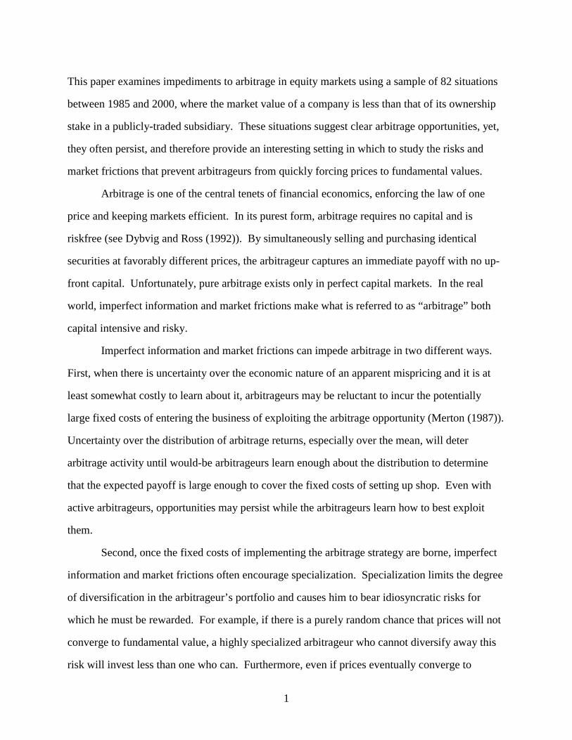
Figure 1 shows the paths of stock prices for both Creative Computers and Ubid. By

December 18, 1998, the discrepancy between Creative Computers and Ubid stock prices had

increased substantially—the value of the stub assets had decreased from negative $28 million to

negative $94 million. Using margin maintenance requirements specified by NYSE and NASD,

the arbitrageur would have faced a margin call and would have been forced to partially liquidate

his position to satisfy maintenance margin requirements.15 The arbitrageur would have lost 26

percent in seven trading days.

[Insert Figure 1 around here]

On December 21, 1998, the value of Creative Computers’ stub assets decreased to

negative $254 million. For a second trading day in a row, the arbitrageur would have faced a

margin call and been forced to reduce his position even further, incurring an additional one-day

loss of 84 percent. Bad luck continued when, on the following trading day, the value of Creative

17

Computers’ stub assets fell to negative $505 million causing a one-day loss of 91 percent. On

December 23, 1998, the value of Creative Computers’ stub assets reached its minimum level of

negative $766 million. The arbitrageur received his fourth and final margin call and an

additional one-day loss of 63 percent.

Figure 1 shows that after December 23, 1998, the prices of Ubid and Creative Computers

converged. As promised by Creative Computers’ management, the remaining Ubid shares were

distributed to Creative Computers’ shareholders six months later. The portion of the

arbitrageur’s capital that was not liquidated returned 150 percent between the peak mispricing on

December 23, 1998 and the spinoff on June 7, 1999. However, because the arbitrageur lost most

of his capital prior to December 23, 1999, his overall return from the Creative Computers/Ubid

investment was negative 99 percent. In order to avoid the costly margin calls, the arbitrageur

would have had to post $4.53 of excess cash for every one dollar of long position. Doing so

would have generated a return of 8.7 percent between December 9, 1998, and June 7, 1999. This

is significantly lower than the 45.9 percent that the arbitrageur could have obtained with the

same initial investment had he not been required to liquidate to meet margin calls.

B.2. Full Sample Results for Individual Investments

The Creative Computers/Ubid example suggests that ignoring margin requirements

results in overestimation of returns from negative-stub-value investments. To determine whether

this is generally the case, we estimate returns for each of the negative-stub-value investments in

our sample using the three leverage levels previously described—textbook leverage (Regulation

T initial margin imposed, no maintenance requirements imposed), Regulation T leverage (both

initial and maintenance margin requirements imposed), and conservative leverage (maximum

asset/equity ratio for which no margin calls are received). Returns are estimated using

investment strategies defined by Rule 1 using buy/sell thresholds of 1.0/0.8, 1.25/1.0, and

1.5/1.0.

18

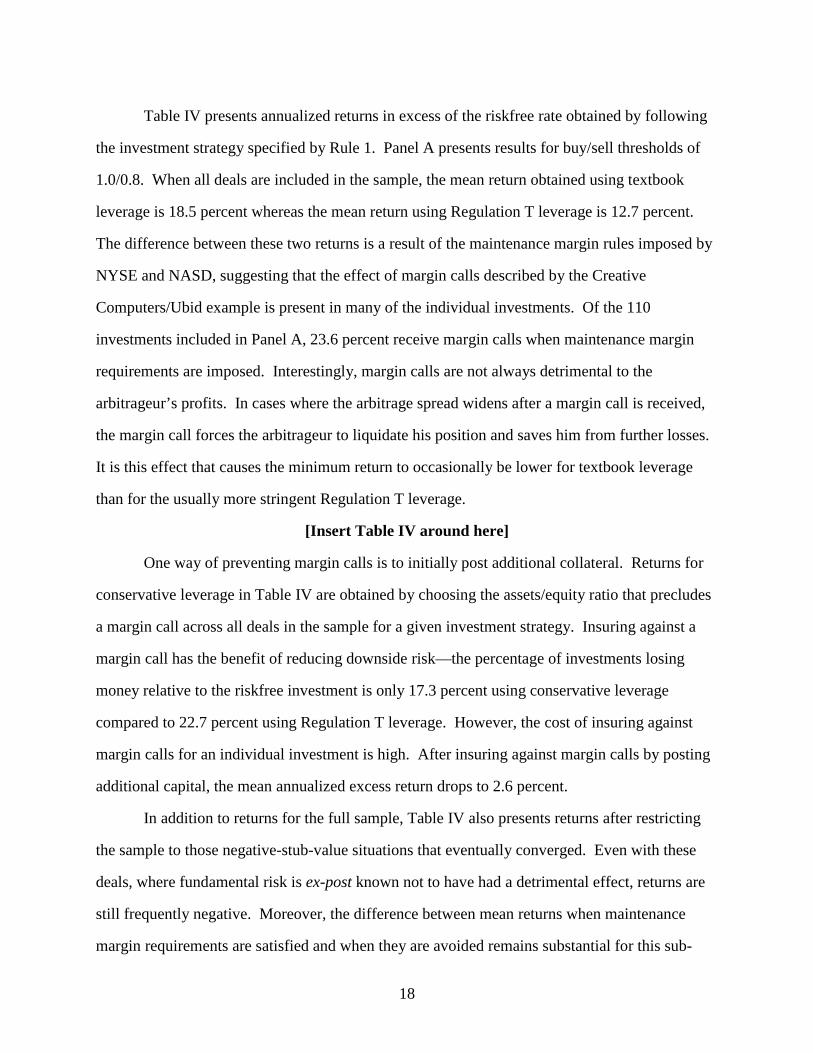
Table IV presents annualized returns in excess of the riskfree rate obtained by following

the investment strategy specified by Rule 1. Panel A presents results for buy/sell thresholds of

1.0/0.8. When all deals are included in the sample, the mean return obtained using textbook

leverage is 18.5 percent whereas the mean return using Regulation T leverage is 12.7 percent.

The difference between these two returns is a result of the maintenance margin rules imposed by

NYSE and NASD, suggesting that the effect of margin calls described by the Creative

Computers/Ubid example is present in many of the individual investments. Of the 110

investments included in Panel A, 23.6 percent receive margin calls when maintenance margin

requirements are imposed. Interestingly, margin calls are not always detrimental to the

arbitrageur’s profits. In cases where the arbitrage spread widens after a margin call is received,

the margin call forces the arbitrageur to liquidate his position and saves him from further losses.

It is this effect that causes the minimum return to occasionally be lower for textbook leverage

than for the usually more stringent Regulation T leverage.

[Insert Table IV around here]

One way of preventing margin calls is to initially post additional collateral. Returns for

conservative leverage in Table IV are obtained by choosing the assets/equity ratio that precludes

a margin call across all deals in the sample for a given investment strategy. Insuring against a

margin call has the benefit of reducing downside risk—the percentage of investments losing

money relative to the riskfree investment is only 17.3 percent using conservative leverage

compared to 22.7 percent using Regulation T leverage. However, the cost of insuring against

margin calls for an individual investment is high. After insuring against margin calls by posting

additional capital, the mean annualized excess return drops to 2.6 percent.

In addition to returns for the full sample, Table IV also presents returns after restricting

the sample to those negative-stub-value situations that eventually converged. Even with these

deals, where fundamental risk is ex-post known not to have had a detrimental effect, returns are

still frequently negative. Moreover, the difference between mean returns when maintenance

margin requirements are satisfied and when they are avoided remains substantial for this sub-

19

sample. In other words, the bumpiness of the path to convergence is costly to the arbitrageur.

This suggests that both horizon risk and margin risk are important for individual investments

even when fundamental risk is mitigated.

Panels B and C of Table IV present results for different buy/sell thresholds, again using

Rule 1 as the investment strategy. Results are similar to those presented in Panel A indicating

that results are not strongly dependent on the levels of the thresholds. Overall, the results

indicate that while annual excess returns from negative-stub-value investments are positive on

average, they are not riskfree.16

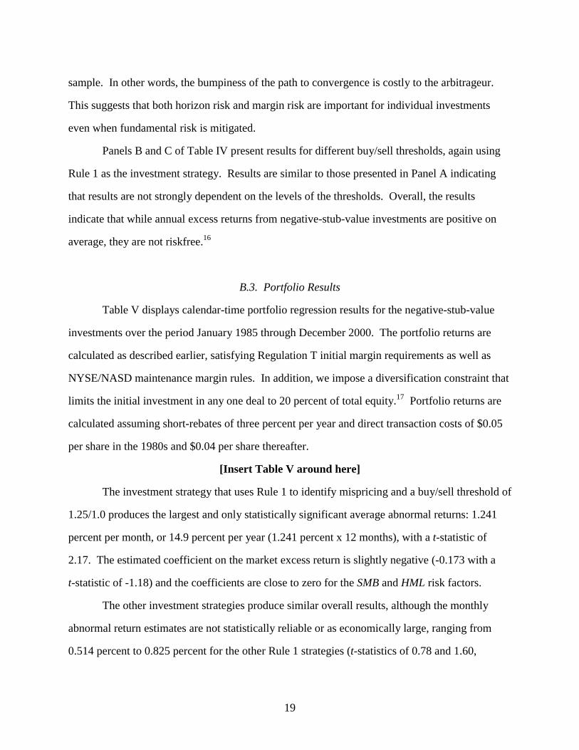
B.3. Portfolio Results

Table V displays calendar-time portfolio regression results for the negative-stub-value

investments over the period January 1985 through December 2000. The portfolio returns are

calculated as described earlier, satisfying Regulation T initial margin requirements as well as

NYSE/NASD maintenance margin rules. In addition, we impose a diversification constraint that

limits the initial investment in any one deal to 20 percent of total equity.17 Portfolio returns are

calculated assuming short-rebates of three percent per year and direct transaction costs of $0.05

per share in the 1980s and $0.04 per share thereafter.

[Insert Table V around here]

The investment strategy that uses Rule 1 to identify mispricing and a buy/sell threshold of

1.25/1.0 produces the largest and only statistically significant average abnormal returns: 1.241

percent per month, or 14.9 percent per year (1.241 percent x 12 months), with a t-statistic of

2.17. The estimated coefficient on the market excess return is slightly negative (-0.173 with a

t-statistic of -1.18) and the coefficients are close to zero for the SMB and HML risk factors.

The other investment strategies produce similar overall results, although the monthly

abnormal return estimates are not statistically reliable or as economically large, ranging from

0.514 percent to 0.825 percent for the other Rule 1 strategies (t-statistics of 0.78 and 1.60,

20

respectively), and from 0.021 percent to 0.745 percent for the Rule 2 strategies (t-statistics of

0.06 and 1.54, respectively).

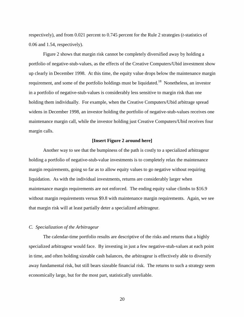
Figure 2 shows that margin risk cannot be completely diversified away by holding a

portfolio of negative-stub-values, as the effects of the Creative Computers/Ubid investment show

up clearly in December 1998. At this time, the equity value drops below the maintenance margin

requirement, and some of the portfolio holdings must be liquidated.18 Nonetheless, an investor

in a portfolio of negative-stub-values is considerably less sensitive to margin risk than one

holding them individually. For example, when the Creative Computers/Ubid arbitrage spread

widens in December 1998, an investor holding the portfolio of negative-stub-values receives one

maintenance margin call, while the investor holding just Creative Computers/Ubid receives four

margin calls.

[Insert Figure 2 around here]

Another way to see that the bumpiness of the path is costly to a specialized arbitrageur

holding a portfolio of negative-stub-value investments is to completely relax the maintenance

margin requirements, going so far as to allow equity values to go negative without requiring

liquidation. As with the individual investments, returns are considerably larger when

maintenance margin requirements are not enforced. The ending equity value climbs to $16.9

without margin requirements versus $9.8 with maintenance margin requirements. Again, we see

that margin risk will at least partially deter a specialized arbitrageur.

C. Specialization of the Arbitrageur

The calendar-time portfolio results are descriptive of the risks and returns that a highly

specialized arbitrageur would face. By investing in just a few negative-stub-values at each point

in time, and often holding sizeable cash balances, the arbitrageur is effectively able to diversify

away fundamental risk, but still bears sizeable financial risk. The returns to such a strategy seem

economically large, but for the most part, statistically unreliable.

21

There are few, if any arbitrage funds that exclusively engage in such an investment

strategy. On the other hand, there are many arbitrage funds that engage in “special situations

arbitrage,” which includes negative-stub-value investments. Although these funds often

specialize in one specific type of arbitrage trade, such as merger arbitrage, they only do so if

there are sufficiently many transactions. This suggests that the specialized arbitrageur described

so far is a bit of a straw man.

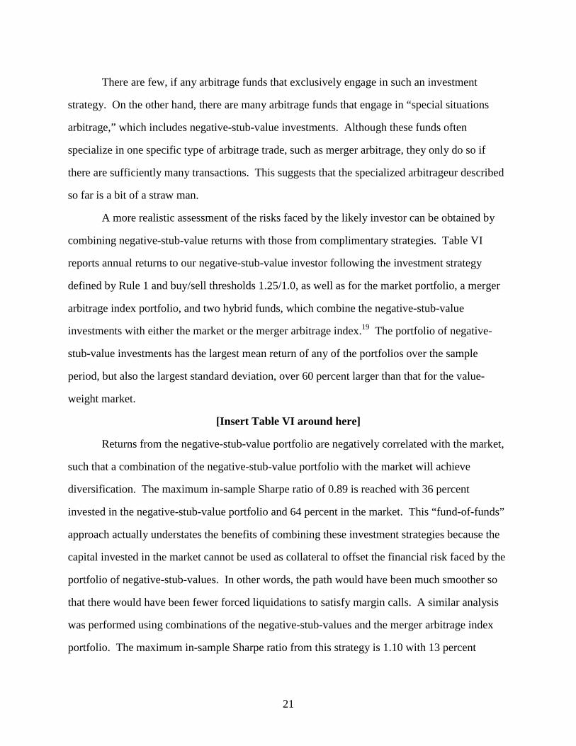
A more realistic assessment of the risks faced by the likely investor can be obtained by

combining negative-stub-value returns with those from complimentary strategies. Table VI

reports annual returns to our negative-stub-value investor following the investment strategy

defined by Rule 1 and buy/sell thresholds 1.25/1.0, as well as for the market portfolio, a merger

arbitrage index portfolio, and two hybrid funds, which combine the negative-stub-value

investments with either the market or the merger arbitrage index.19 The portfolio of negative-

stub-value investments has the largest mean return of any of the portfolios over the sample

period, but also the largest standard deviation, over 60 percent larger than that for the value-

weight market.

[Insert Table VI around here]

Returns from the negative-stub-value portfolio are negatively correlated with the market,

such that a combination of the negative-stub-value portfolio with the market will achieve

diversification. The maximum in-sample Sharpe ratio of 0.89 is reached with 36 percent

invested in the negative-stub-value portfolio and 64 percent in the market. This “fund-of-funds”

approach actually understates the benefits of combining these investment strategies because the

capital invested in the market cannot be used as collateral to offset the financial risk faced by the

portfolio of negative-stub-values. In other words, the path would have been much smoother so

that there would have been fewer forced liquidations to satisfy margin calls. A similar analysis

was performed using combinations of the negative-stub-values and the merger arbitrage index

portfolio. The maximum in-sample Sharpe ratio from this strategy is 1.10 with 13 percent

22

invested in the negative-stub-value portfolio and 87 percent in the merger arbitrage index

portfolio.

This suggests that fundamental and margin risks, which are clearly important for

someone investing in individual negative-stub-values, are less likely to create a serious

impediment to the likely arbitrageur of these relative mispricings.

V. Arbitrage in Imperfect Capital Markets

A. Costs of Short Selling and Buy-In Risk

In addition to the risks discussed above, the persistence of the mispricing in negative-

stub-value situations may be the result of short-selling frictions (see Lamont and Thaler (2001)).

The arbitrage strategy requires selling short shares in the subsidiary firm, which generally have

low public floats. In other words, the percentage of outstanding shares available to be publicly-

traded is small because the parent firms, and often the firms’ managers, own the vast majority of

the shares. As a result, the number of marginable shares that can be sold short may be low.

One indication that short selling may be costly is shown by the “short-rebate.” Short-

rebate refers to the interest rate that investors are paid on the proceeds they obtain from

borrowing and selling a stock. Generally, institutional investors are paid 25 to 50 basis points

below the federal funds rate on short proceeds, but this discount can vary, and occasionally the

short-rebate is negative. That is, in addition to keeping the interest on the investor’s short

proceeds, the broker sometimes charges the investor to maintain the short position.

Of course, the short-rebate is a market price, representing both supply and demand. To

understand the market for selling short shares, we talked with several industry practitioners and

obtained short-rebate data from Ameritrade Holding Corporation, a large retail on-line brokerage

firm. All indications are that this is a very active and liquid market (see D’Avolio (2001) and

Geczy, Musto, and Reed (2001)). The stock-loan department at Ameritrade lends shares out of

its customers’ margin accounts to large investment houses and hedge funds. If an investment

house such as Goldman Sachs is unable to provide shares to loan to a client short seller out of its

23

own customers’ accounts or its proprietary account, they will try to borrow the shares from

another institution such as State Street Bank or from a broker-dealer, such as Ameritrade.

Table VII displays summary statistics of the Ameritrade short-rebate data set. During the

December 1998 through October 2000 period for which short-rebate data are available, there are

28 firms in our sample that qualify under Rule 1 with a buy threshold 1.0. Of these 28 firms, 24

(85.7 percent) are in the Ameritrade database. Six (25 percent) of the firms in the Amertrade

database have negative rebates. As displayed in Table VII, similar patterns exist for the other

buy thresholds and for Rule 2. We also note that out of roughly 10,000 NYSE, AMEX, and

Nasdaq stocks during the December 1998 through October 2000 interval, there are a total of 48

firms in the Ameritrade database that have negative short-rebates. Of these 48 firms, seven (15

percent) are from our sample. Clearly, the price for selling short the subsidiary shares is high

relative to the typical firm.

[Insert Table VII around here]

Panel B of Table VII reports the minimum short-rebates paid for subsidiary shares

reported for each subsidiary firm in the Ameritrade database. The data show that the minimum

short-rebate transaction prices tend to be close to zero, suggesting that negative short-rebates are

unlikely to be the full story behind the persistence of negative-stub-values. Excluding the two

most extreme observations, the minimum short-rebates range from negative eight percent to six

percent per year, with the median short-rebate of one percent.

Consider the case of the most extreme negative short-rebate in the sample, Stratos

Lightwave. According to the data, an arbitrageur wishing to exploit the relative mispricing of

Methode/Stratos Lightwave would have been charged a 40 percent annual interest rate on short

proceeds from short selling Stratos Lightwave. Following the investment strategy described by

Rule 1 and buy/sell threshold of 1.25/1.0, the arbitrageur would have invested in the deal on July

11, 2000, and would have still been invested at the end of the year. Over this period, the equity

value of the position increased 21.1 percent before including the effects of the negative short-

rebate.20 However, after paying nearly six months of negative short-rebate, the arbitrageur’s

24

return is reduced to negative 0.6 percent. This example highlights that the real impediment is not

the short-rebate, but instead the uncertainty over how long you will be paying it. In other words,

an arbitrageur should be more than willing to pay a short-rebate of negative 100 percent per year

if he can correct a 25 percent mispricing in a week.

When shares available for shorting are most scarce, brokers cannot maintain their client’s

short positions no matter what interest rate the investor is willing to pay. This situation, which

arises when owners of the stock demand that their loaned-out shares be returned, is often referred

to as being “bought-in.” Of the 24 negative-stub-value trades in the Ameritrade short-rebate

database, identified using Rule 1 and a buy threshold of 1.0, three were partially bought-in before

the arbitrage spread converged. Similar results are found for Rule 2 and other buy thresholds.

Moreover, casual empiricism suggests that the risk of being bought-in is greatest when the

arbitrage spreads of several negative-stub-value investments have widened, suggesting that this

risk may not be completely idiosyncratic. The possibility of being bought-in at an unattractive

price provides a disincentive for arbitrageurs to take a large position and represents a substantial

friction to executing the arbitrage trade.

B. Imperfect Information and the Persistence of Negative-Stub-Values

So why do negative-stub-values persist? To gain perspective on this question, it may be

important to consider the details of this particular mispricing phenomenon. Merton (1987)

argues that one must be careful when drawing inferences about market anomalies relative to a

perfect capital market because imperfections, especially imperfect information, can induce

serious distortions. We believe this to be the case for this sample.

First, there is enormous uncertainty over the economic nature of the apparent mispricing

and it will take time to learn about it. Uncertainty over the distribution of returns makes it

difficult to know whether the arbitrage trades will on average be worthwhile investments, and

how they should best be exploited. In other words, at the onset, it is not known whether the

25

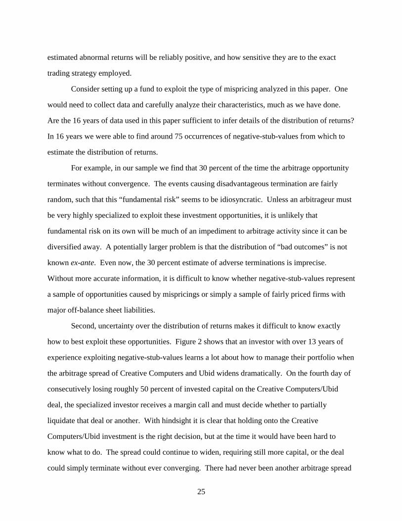
estimated abnormal returns will be reliably positive, and how sensitive they are to the exact

trading strategy employed.

Consider setting up a fund to exploit the type of mispricing analyzed in this paper. One

would need to collect data and carefully analyze their characteristics, much as we have done.

Are the 16 years of data used in this paper sufficient to infer details of the distribution of returns?

In 16 years we were able to find around 75 occurrences of negative-stub-values from which to

estimate the distribution of returns.

For example, in our sample we find that 30 percent of the time the arbitrage opportunity

terminates without convergence. The events causing disadvantageous termination are fairly

random, such that this “fundamental risk” seems to be idiosyncratic. Unless an arbitrageur must

be very highly specialized to exploit these investment opportunities, it is unlikely that

fundamental risk on its own will be much of an impediment to arbitrage activity since it can be

diversified away. A potentially larger problem is that the distribution of “bad outcomes” is not

known ex-ante. Even now, the 30 percent estimate of adverse terminations is imprecise.

Without more accurate information, it is difficult to know whether negative-stub-values represent

a sample of opportunities caused by mispricings or simply a sample of fairly priced firms with

major off-balance sheet liabilities.

Second, uncertainty over the distribution of returns makes it difficult to know exactly

how to best exploit these opportunities. Figure 2 shows that an investor with over 13 years of

experience exploiting negative-stub-values learns a lot about how to manage their portfolio when

the arbitrage spread of Creative Computers and Ubid widens dramatically. On the fourth day of

consecutively losing roughly 50 percent of invested capital on the Creative Computers/Ubid

deal, the specialized investor receives a margin call and must decide whether to partially

liquidate that deal or another. With hindsight it is clear that holding onto the Creative

Computers/Ubid investment is the right decision, but at the time it would have been hard to

know what to do. The spread could continue to widen, requiring still more capital, or the deal

could simply terminate without ever converging. There had never been another arbitrage spread

26

that had widened so much so quickly, and one would surely be questioning whether they had

missed something important in their analysis. The opportunity to learn presents itself again one

year later when 11 out of 15 arbitrage spreads widen over a three-week period. Again, there is

little in the data that could have prepared the investor for this outcome, as this was the first time

that so many negative-stub-values existed at one time. What at first may have seemed like an

opportunity to diversify, turns out to drive the equity value of the portfolio negative.

Another way to see that there is considerable uncertainty about the outcomes of negative-

stub-values is to examine stock price reactions around announcements of news concerning

distributions and the IRS tax treatments of these transactions. Specifically, we identify

announcements of (1) the intent of parent to eventually distribute subsidiary shares to

shareholders, (2) a tentative or definitive date for distribution, and (3) IRS approval of

distribution as a tax-free transaction.21 Table VIII reports mean and median stock price reactions

to the release of this information using three-day event windows. The dates of the information

releases are collected from the Wall Street Journal and the Dow Jones News Retrieval Service.

Sixteen of the sample firms had at least one news story discussing a “distribution” or the “IRS.”

The average stock price reaction to the release of this information was 6.17 percent for the parent

firm (t-statistic = 2.64) and -2.25 percent for the subsidiary (t-statistic = -0.95). The average

three-day return for the net long-short position held by an arbitrageur is 8.29 percent (t-statistic =

3.25) and the median return is 9.39 percent (p-value = 0.0097). Importantly, stock price

reactions tend to be just as large for firms that had previously indicated their intention to

distribute the subsidiary shares to shareholders in their prospectus as for the firms that reveal this

intention for the first time.

[Insert Table VIII around here]

It is also interesting to note that the reaction is larger for the firms where the mispricing

ratio initially indicates a negative-stub-value. Using Rule 1, many of the negative-stub-values

have converged prior to these announcements, but for the firms that still have a negative-stub,

the average stock price reaction is 11.37 percent and the median is 10.85 percent. For this

27

subsample, where Rule 1 indicates a mispricing prior to the announcement, the median

mispricing ratio falls from 1.11 before the announcement to 1.01 immediately after the

announcement.22 In other words, with no change in the availability of shares for shorting, no

modifications to the rules governing capital requirements, and no reduction in direct transaction

costs, virtually all of the mispricing is immediately eliminated once the uncertainty over the

outcome is resolved.

Finally, we note that our assessment of the risks associated with investing in negative-

stub-value situations is based on the entire history of these trades, from 1985 through the end of

2000. An arbitrageur investing at any point during the sample period would not have had the

benefit of seeing as much data. Stated differently, the arbitrageur’s estimates of the risks

associated with negative-stub-value investments almost surely would have been less precise than

those presented in this paper. This added uncertainty provides another impediment to arbitrage

and also helps to explain the persistence of seemingly obvious mispricings.

VI. Conclusion

This paper studies the impediments to arbitraging relative mispricings of corporate cross

holdings, where the parent firm is worth less than its ownership stake in a publicly-traded

subsidiary. We find that there are costs that limit arbitrage in equity markets, which tests our

faith in market forces keeping prices at fundamental values.23

The biggest friction impeding arbitrage appears to be the costs associated with imperfect

information (Merton (1987) and Fama (1991)).24 In order for arbitrage to keep prices at

fundamental values, the arbitrageur must have a reasonable understanding of the economic

situation. Becoming informed about negative-stub-value investing is difficult when there is little

evidence to examine. Furthermore, the ex-ante benefits from becoming informed are not known.

Expected payoffs will be large only if there are numerous opportunities or the magnitude of the

opportunities is large. Over a 16-year period, we are able to identify fewer than 100 negative-

stub-value situations. The total amount of capital that can be employed in this investment

28

strategy is low since the effective size (controlling for the public float) of the subsidiary tends to

be very small.

In addition, imperfect information and transaction costs may encourage at least some

specialization of arbitrageurs, which limits the effectiveness of diversification. Because poorly

diversified investors will require compensation for idiosyncratic risks, fundamental risks

associated with negative-stub-values can limit arbitrage activity. Even more serious are the

financial risks borne by highly specialized arbitrageurs. As we show, the returns to a highly

specialized arbitrageur investing in negative-stub-values would be 50 percent to 100 percent

larger if capital requirements were relaxed. This drives a large wedge between the range of

prices that will be arbitraged away in imperfect capital markets versus those in perfect capital

markets.

Finally, to the extent that the initial mispricing is due to noise traders bidding up the

subsidiary share prices, we can say something about their long-term prospects with respect to

this event. Arbitrageurs’ profits are made at the expense of the investors who are long the

subsidiary’s stock. The abnormal returns to an equal-weight portfolio that is long parent firms

are zero, while the abnormal returns to an equal-weight portfolio that is long subsidiary firms are

reliably negative. This suggests that the subsidiary shares somehow become overpriced before

arbitrageurs force them back down to fundamental values. Thus, the evidence is consistent with

the arguments of Friedman (1953) and Fama (1965) that investors who make mistakes will

experience losses and over time will be driven out of the market. Market forces are working

hard to keep prices at fundamental values, but the effectiveness of these efforts is sometimes

limited.

29

REFERENCES

Andrade, Gregor, Stuart Gilson, and Todd Pulvino, 2001, Seagate technology buyout, Casestudy,

Harvard Business School.

Brav, Alon, and J. B. Heaton, 2002, Competing theories of financial anomalies, Review of

Financial Studies, forthcoming.

Cornell, Bradford, and Qiao Liu, 2000, The parent company puzzle: When the whole is worth

less than one of the parts? UCLA Working paper.

Cornell, Bradford, and Alan Shapiro, 1989, The mispricing of U.S. Treasury bonds, Review of

Financial Studies 3, 297-310.

D’Avolio, Gene, 2001, The market for borrowing stocks, Harvard University Working paper.

Dammon, Robert M., Kenneth B. Dunn, and Chester S. Spatt, 1993, The relative pricing of high-

yield debt: The case of RJR Nabisco Holdings Capital Corporation, American Economic

Review 83, 1090-1111.

DeLong, J. Bradford, Andrei Shleifer, Lawrence Summers, and Robert Waldman, 1990, Noise

trader risk in financial markets, Journal of Political Economy 98, 703-738.

Dybvig, Phillip H. and Stephen A. Ross, 1992, Arbitrage, in John Eatwell, Murray Milgate, and

Peter Newman, eds.: The New Palgrave Dictionary of Money and Finance (MacMillan:

London; Stockton Press: New York).

Fama, Eugene F., 1965, The behavior of stock market prices, Journal of Business 38, 34-105.

Fama, Eugene F., 1991, Efficient capital markets: II, Journal of Finance 46, 1575-1617.

30

Fama, Eugene F., and Kenneth R. French, 1993, Common risk factors in the returns on stocks

and bonds, Journal of Financial Economics 33, 3-56.

Friedman, Milton, 1953, The case for flexible exchange rates, in Essays in Positive Economics

(University of Chicago Press, Chicago, IL).

Geczy, Christopher, David Musto, and Adam Reed, 2001, Stocks are special too: An analysis of

the equity lending market, Wharton Working paper.

Green, Richard C., and Kristian Rydqvist, 1997, The valuation of non-systematic risks and the

pricing of Swedish lottery bonds, Review of Financial Studies 10, 447-480.

Jarrow, Robert, and Maureen O’Hara, 1989, Primes and scores: An essay on market

imperfections, Journal of Finance 44, 1263-1287.

Lamont, Owen, and Richard Thaler, 2001, Can the market add and subtract? Mispricing in tech

stock carve-outs, University of Chicago Working paper.

Lee, Charles, Andrei Shleifer, and Richard Thaler, 1991, Investor sentiment and the closed-end

fund puzzle, Journal of Finance 46, 75-109.

Liu, Jun and Francis Longstaff, 2000, Losing money on arbitrages: Optimal dynamic portfolio

choice in markets with arbitrage opportunities, UCLA Working paper.

Longstaff, Francis, 1992, Are negative option prices possible? The callable U.S. Treasury-Bond

puzzle, Journal of Business 65, 571-592.

Merton, Robert C., 1987, A simple model of capital market equilibrium with incomplete

information, Journal of Finance 42, 483-511.

Mitchell, Mark, and Todd Pulvino, 2001, Characteristics of risk and return in risk arbitrage,

Journal of Finance, forthcoming.

31

PFSWeb Initial Public Offering Prospectus, December 2, 1999, U.S. Securities and Exchange

Commission.

Pulvino, Todd, and Ashish Das, 1999, Ubid, Casestudy, Kellogg Graduate School of

Management.

Rosenthal, Leonard, and Colin Young, 1990, The seemingly anomalous price behavior of Royal

Dutch / Shell and Unilever N.V. / PLC, Journal of Financial Economics 26, 123-141.

Schill, Michael, and Chunsheng Zhou, 2000, Pricing an emerging industry: Evidence from

internet subsidiary carve-outs, University of California Riverside Working paper.

Shleifer, Andrei, and Lawrence Summers, 1990, The noise trader approach to finance, Journal of

Economic Perspectives 4, 19-33.

Shleifer, Andrei, and Robert Vishny, 1997, The limits of arbitrage, Journal of Finance 52, 35-55.

Tezel, Ahmet, and Oliver Schnusenberg, 2000, Split-off IPOs: Market returns and efficiency, St.

Joseph’s University Working paper.

32

1 Throughout this paper, we refer to the company in which the parent holds an ownership stake

as a subsidiary, even though the parent may not own more than 50 percent of the company's

voting stock.

2 Cornell and Liu (2000), Lamont and Thaler (2000), Schill and Zhou (2000), and Tezel and

Schnusenberg (2000) examine 10 negative-stub-values during 1998 through 2000. They

conclude that high demand for a limited number of subsidiary shares coupled with short sale

constraints produce irrationally high prices. Relative mispricings in other markets have been

studied by many authors, for example, Cornell and Shapiro (1989), Jarrow and O’Hara (1989),

Rosenthal and Young (1990), Lee, Shleifer, and Thaler (1991), Longstaff (1992); Dammon,

Dunn, and Spatt (1993), and Green and Rydqvist (1997).

3 Another potential liability is the capital gains tax arising from the distribution of the subsidiary

shares to the existing parent firm shareholders. In general, to qualify for a tax-free distribution

the subsidiary business must have been in existence for at least five years and the parent firm

must control at least 80 percent of the subsidiary voting shares. However, the 80 percent

ownership rule can be circumvented. For example, the parent firm can create a new entity that

buys the non-subsidiary assets and then the subsidiary firm can acquire the remaining parent

assets in a tax-free stock merger, effectively distributing the subsidiary shares to existing parent

firm shareholders (see Andrade, Gilson, and Pulvino (2001)).

4 Collecting shares outstanding data in this way ensures that errors in CRSP’s daily shares

outstanding do not affect our return calculations.

5 The Securities Exchange Act of 1934 granted the power to establish initial margin requirements

to the Federal Reserve Board, which on October 1, 1934 instituted Regulation T. Since 1934,

Regulation T has been amended numerous times, primarily to change the initial margin

requirement. Regulation T was last amended in 1974 when the initial margin requirement was

set at 50 percent.

33

6 There are special margin requirements for shorting stocks that have a price less than five

dollars. For stocks priced between and including $2.50 and $5.00, the maintenance margin

requirement is 100 percent. For stocks priced below $2.50, the maintenance requirement is

$2.50 per share shorted.

7 Note that brokerage firms typically impose higher maintenance requirements for retail investors

than the maintenance requirements stipulated by the NYSE and NASD. For example, Charles

Schwab & Co. has a minimum maintenance requirement of 35 percent for long positions. In

addition, brokerage firms often set higher initial and maintenance margin requirements for

certain securities depending on volatility. In all cases, the higher requirement, whether imposed

by the Federal Reserve Board, the exchange/self-regulatory organization, or the broker, prevails.

8 The short-rebate estimate of three percent reflects a discount from the more typical rate of 50

basis points below the federal funds rate. Section V discusses short-rebates in more detail.

9 PFSWeb IPO prospectus, December 2, 1999, pp. 10.

10 This calculation assumes that 50 percent of the long position and 50 percent of the short

position (per Regulation T) was posted as collateral.

11 Ultimately, Howmet's board rejected Cordant's $17 offer and on March 13, 2000 Alcoa offered

to buy Cordant Technologies for $57 per share in cash. It also announced its intention to buy

Howmet's publicly-traded shares. As of March 22, 2000, assuming the arbitrageur had the

foresight, fortitude, and financial resources necessary to hold his position, his investment in

Howmet and Cordant on November 11, 1999 would have returned 35 percent in four months.

12 Liu and Longstaff (2000) examine horizon risk and margin risk in bond arbitrage strategies.

They show that it is often optimal for investors to refrain from taking the maximum position

allowed by margin constraints, even when the arbitrage spread is guaranteed to converge in the

future.

34

13 See Pulvino and Das (1999) for a case study on Creative Computers' carve-out of Ubid.

14 Throughout this example, we assume that the arbitrageur does not earn interest on his posted

collateral or short proceeds. In the full sample analyses that follow, we assume that cash

balances earn the Treasury bill rate and short proceeds earn three percent.

15 Alternatively, the arbitrageur could contribute additional capital. However, allowing the

arbitrageur to do this would imply that a pool of capital had been allocated, ex-ante, to meet

margin calls. Thus, the denominator in the return calculation should include this pool of reserve

capital. To avoid this, we assume that the arbitrageur partially liquidates his position in response

to margin calls. This assumption has the effect of decreasing calculated returns if the subsequent

arbitrage spread converges, and increasing calculated returns if subsequent arbitrage spreads

widen.

16 We repeated the analysis presented in Table IV using Rule 2 to identify mispricing (results not

reported). This change in the investment strategy has only a small effect on the results

suggesting that the risks and returns are not overly sensitive to the method used to quantify the

mispricing.

17 We originally chose the 20 percent diversification constraint as a reasonable level that an

arbitrageur might choose. Subsequent analyses coincidentally showed that 20 percent is the level

of diversification that maximizes portfolio returns over the sample period.

18 Positions are liquidated randomly to satisfy margin calls. Chance had this particular

investment strategy liquidate a position other than Creative Computers/Ubid to cover the margin

call. This proved fortunate for the arbitrageur as the Creative Computers/Ubid investment

experienced a huge return on the very next day causing the equity value of the portfolio to

increase 46.2 percent.

35

19 Merger arbitrage index returns are obtained from the analysis described in Mitchell and

Pulvino (2001).

20 This calculation assumes the maximum initial leverage allowed by Regulation T and ignores

net interest on cash and debit balances.

21 Often these announcements are made simultaneously.

22 The mean mispricing ratio falls from 1.12 before the announcement to 1.02 after the

announcement.

23 We thank Ken French for discussions on this issue.

24 See also Brav and Heaton (2002).

36

Figure 1. Paths of Stock Prices for Creative Computers and Ubid

$0

$20

$40

$60

$80

$100

$120

$140

$160

12/1/98 1/1/99 2/1/99 3/1/99 4/1/99 5/1/99 6/1/99

Shar

e Pr

ice

Ubid (x .72)

CreativeComputers

Invest12/9/98

Margin Call #112/18/98

Margin Call #212/21/98

Margin Call #3 12/22/98

Margin Call #4 12/23/98

37

Figure 2. Daily Portfolio Values of Negative-Stub Investments Ignoring Maintenance Margin Requirements.This figure shows the value of one dollar invested at the beginning of the period from 1986 to 2000 in negative-stub-value investments. Negative-stub-valueportfolio values are obtained from an investment strategy based on Rule 1 (below) using a buy threshold of 1.25 and a sell threshold of 1.0:

1.0 iftradeTerminate and 25.1iftradePlace

<>EquityParent

Stake

EquityParent

Stake

MVMV

MVMV .

The portfolio value calculation cumulates daily payoffs from the arbitrage positions and ignores maintenance capital requirements, allowing the value of investedcapital to become negative.

-$10

-$5

$0

$5

$10

$15

$20

9/12/86 9/12/88 9/12/90 9/12/92 9/12/94 9/12/96 9/12/98 9/12/00

Port

folio

Val

ue

$1 Initial Investment

Creative Computers / Ubid Spread Widens

11 out of 15 Spreads Widen

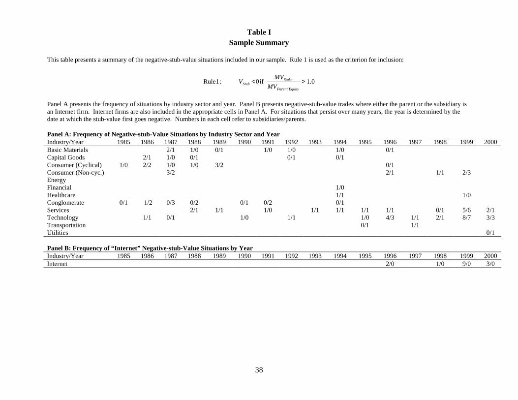
38

Table ISample Summary

This table presents a summary of the negative-stub-value situations included in our sample. Rule 1 is used as the criterion for inclusion:

0.1if0:1Rule

><EquityParent

StakeStub MV

MVV

Panel A presents the frequency of situations by industry sector and year. Panel B presents negative-stub-value trades where either the parent or the subsidiary isan Internet firm. Internet firms are also included in the appropriate cells in Panel A. For situations that persist over many years, the year is determined by thedate at which the stub-value first goes negative. Numbers in each cell refer to subsidiaries/parents.

Panel A: Frequency of Negative-stub-Value Situations by Industry Sector and YearIndustry/Year 1985 1986 1987 1988 1989 1990 1991 1992 1993 1994 1995 1996 1997 1998 1999 2000Basic Materials 2/1 1/0 0/1 1/0 1/0 1/0 0/1Capital Goods 2/1 1/0 0/1 0/1 0/1Consumer (Cyclical) 1/0 2/2 1/0 1/0 3/2 0/1Consumer (Non-cyc.) 3/2 2/1 1/1 2/3EnergyFinancial 1/0Healthcare 1/1 1/0Conglomerate 0/1 1/2 0/3 0/2 0/1 0/2 0/1Services 2/1 1/1 1/0 1/1 1/1 1/1 1/1 0/1 5/6 2/1Technology 1/1 0/1 1/0 1/1 1/0 4/3 1/1 2/1 8/7 3/3Transportation 0/1 1/1Utilities 0/1

Panel B: Frequency of “Internet” Negative-stub-Value Situations by YearIndustry/Year 1985 1986 1987 1988 1989 1990 1991 1992 1993 1994 1995 1996 1997 1998 1999 2000Internet 2/0 1/0 9/0 3/0

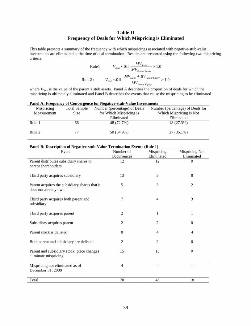
39

Table IIFrequency of Deals for Which Mispricing is Eliminated

This table presents a summary of the frequency with which mispricings associated with negative-stub-valueinvestments are eliminated at the time of deal termination. Results are presented using the following two mispricingcriteria:

0.1if0:1Rule

><EquityParent

StakeStub MV

MVV

0.1if0:2Rule

>+

<EquityParent

EquityParentStakeStub MV

BVMVV

where VStub is the value of the parent’s stub assets. Panel A describes the proportion of deals for which themispricing is ultimately eliminated and Panel B describes the events that cause the mispricing to be eliminated.

Panel A: Frequency of Convergence for Negative-stub-Value InvestmentsMispricing

MeasurementTotal Sample

SizeNumber (percentage) of Deals

for Which Mispricing isEliminated

Number (percentage) of Deals forWhich Mispricing is Not

EliminatedRule 1 66 48 (72.7%) 18 (27.3%)

Rule 2 77 50 (64.9%) 27 (35.1%)

Panel B: Description of Negative-stub-Value Termination Events (Rule 1)Event Number of

OccurrencesMispricingEliminated

Mispricing NotEliminated

Parent distributes subsidiary shares toparent shareholders

12 12 0

Third party acquires subsidiary 13 5 8

Parent acquires the subsidiary shares that itdoes not already own

5 3 2

Third party acquires both parent andsubsidiary

7 4 3

Third party acquires parent 2 1 1

Subsidiary acquires parent 2 2 0

Parent stock is delisted 8 4 4

Both parent and subsidiary are delisted 2 2 0

Parent and subsidiary stock price changeseliminate mispricing

15 15 0

Mispricing not eliminated as ofDecember 31, 2000

4 --- ---

Total 70 48 18

40

Table IIIInvestment Horizon

This table presents a summary of the number of days invested using two different trading strategies. Panels A and Bshow the number of days invested using Rule 1, for the full sample and for converged deals, respectively. Rule 1 isdefined as:

Threshold.Sell iftradeTerminate and ThresholdBuyiftradePlace

<>EquityParent

Stake

EquityParent

Stake

MVMV

MVMV

Panels B and D show the number of days invested using Rule 2 for the full sample and for converged deals, whereRule 2 is defined as:

Threshold.Sell iftradeTerminate

ThresholdBuyiftradePlace

<+

>+

EquityParent

EquityParentStake

EquityParent

EquityParentStake

MVBVMV

MVBVMV

Converged deals are identified as those where the mispricing ratio is smaller at termination than at the initial date.Results are presented for various buy and sell thresholds. Table entries, other than buy and sell thresholds, representtrading days.

Panel A: Number of Days Invested Using Rule 1 for all InvestmentsPercentile

BuyThreshold

SellThreshold

Number ofInvestments

Minimum 25th 50th 75th Maximum Mean

1.00 0.8 110 1.0 29.0 92.0 274.0 2,796.0 236.31.25 1.0 75 2.0 28.5 84.0 213.0 2,413.0 214.41.50 1.0 39 13.0 92.5 159.0 258.3 2,370.0 343.1

Panel B: Number of Days Invested Using Rule 1 for Converged InvestmentsPercentile

BuyThreshold

SellThreshold

Number ofInvestments

Minimum 25th 50th 75th Maximum Mean

1.00 0.8 79 3.0 25.0 74.0 207.5 1,804.0 176.51.25 1.0 40 2.0 26.5 66.5 127.5 1,792.0 164.71.50 1.0 20 13.0 46.0 117.5 163.0 1,792.0 265.9

Panel C: Number of Days Invested Using Rule 2 for all InvestmentsPercentile

BuyThreshold

SellThreshold

Number ofInvestments

Minimum 25th 50th 75th Maximum Mean

1.00 0.8 130 3.0 46.0 155.5 380.0 2,818.0 309.71.25 1.0 119 3.0 41.5 114.0 285.0 2,818.0 236.01.50 1.0 67 7.0 68.8 182.0 336.0 2,804.0 327.7

Panel D: Number of Days Invested Using Rule 2 for Converged InvestmentsPercentile

BuyThreshold

SellThreshold

Number ofInvestments

Minimum 25th 50th 75th Maximum Mean

1.00 0.8 94 3.0 35.0 109.0 279.0 2,818.0 271.11.25 1.0 79 4.0 34.3 68.0 229.3 2,818.0 205.21.50 1.0 41 7.0 55.0 100.0 278.8 2,804.0 290.5

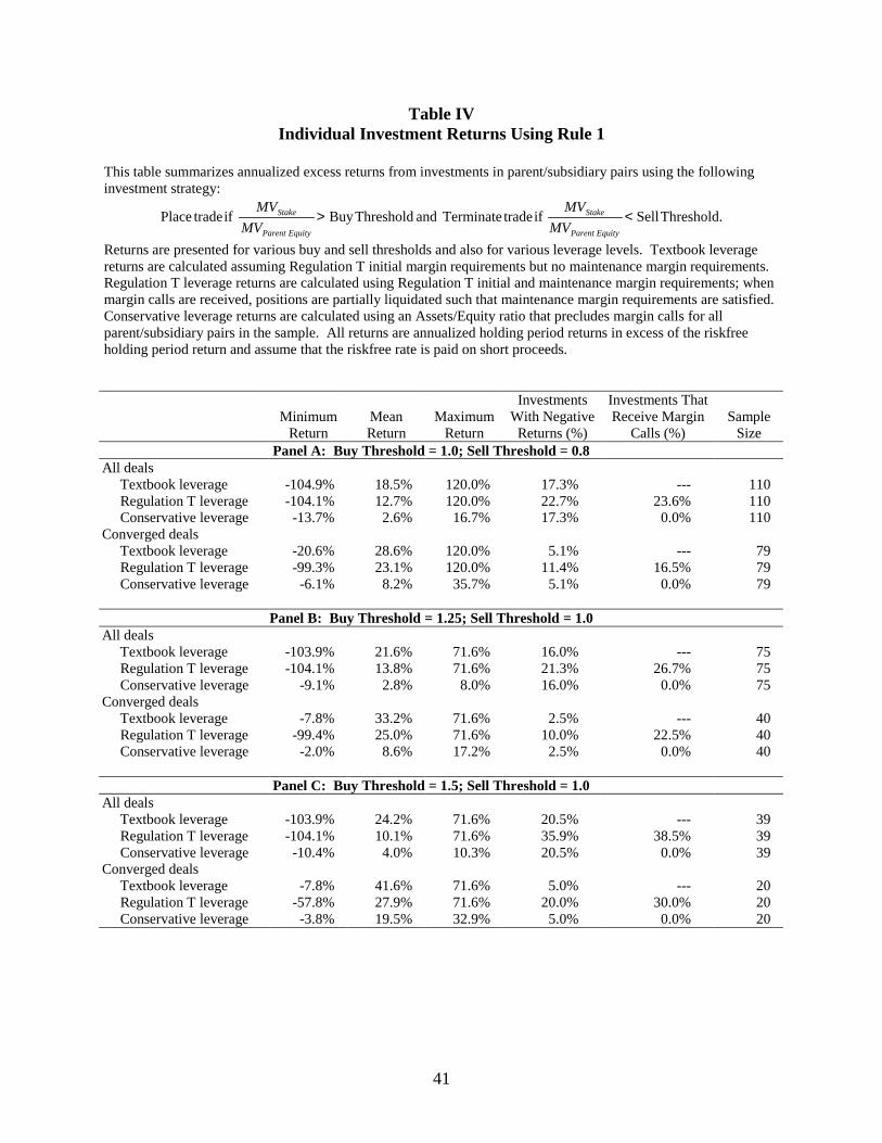
41

Table IVIndividual Investment Returns Using Rule 1

This table summarizes annualized excess returns from investments in parent/subsidiary pairs using the followinginvestment strategy:

Threshold.Sell iftradeTerminate and ThresholdBuyiftradePlace

<>EquityParent

Stake

EquityParent

Stake

MVMV

MVMV

Returns are presented for various buy and sell thresholds and also for various leverage levels. Textbook leveragereturns are calculated assuming Regulation T initial margin requirements but no maintenance margin requirements.Regulation T leverage returns are calculated using Regulation T initial and maintenance margin requirements; whenmargin calls are received, positions are partially liquidated such that maintenance margin requirements are satisfied.Conservative leverage returns are calculated using an Assets/Equity ratio that precludes margin calls for allparent/subsidiary pairs in the sample. All returns are annualized holding period returns in excess of the riskfreeholding period return and assume that the riskfree rate is paid on short proceeds.

MinimumReturn

MeanReturn

MaximumReturn

InvestmentsWith Negative

Returns (%)

Investments ThatReceive Margin

Calls (%)Sample

SizePanel A: Buy Threshold = 1.0; Sell Threshold = 0.8

All deals Textbook leverage -104.9% 18.5% 120.0% 17.3% --- 110 Regulation T leverage -104.1% 12.7% 120.0% 22.7% 23.6% 110 Conservative leverage -13.7% 2.6% 16.7% 17.3% 0.0% 110Converged deals Textbook leverage -20.6% 28.6% 120.0% 5.1% --- 79 Regulation T leverage -99.3% 23.1% 120.0% 11.4% 16.5% 79 Conservative leverage -6.1% 8.2% 35.7% 5.1% 0.0% 79

Panel B: Buy Threshold = 1.25; Sell Threshold = 1.0All deals Textbook leverage -103.9% 21.6% 71.6% 16.0% --- 75 Regulation T leverage -104.1% 13.8% 71.6% 21.3% 26.7% 75 Conservative leverage -9.1% 2.8% 8.0% 16.0% 0.0% 75Converged deals Textbook leverage -7.8% 33.2% 71.6% 2.5% --- 40 Regulation T leverage -99.4% 25.0% 71.6% 10.0% 22.5% 40 Conservative leverage -2.0% 8.6% 17.2% 2.5% 0.0% 40

Panel C: Buy Threshold = 1.5; Sell Threshold = 1.0All deals Textbook leverage -103.9% 24.2% 71.6% 20.5% --- 39 Regulation T leverage -104.1% 10.1% 71.6% 35.9% 38.5% 39 Conservative leverage -10.4% 4.0% 10.3% 20.5% 0.0% 39Converged deals Textbook leverage -7.8% 41.6% 71.6% 5.0% --- 20 Regulation T leverage -57.8% 27.9% 71.6% 20.0% 30.0% 20 Conservative leverage -3.8% 19.5% 32.9% 5.0% 0.0% 20

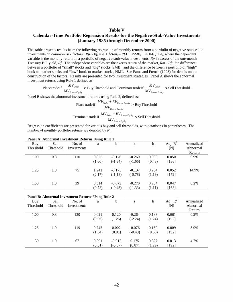
42

Table VCalendar-Time Portfolio Regression Results for the Negative-Stub-Value Investments

(January 1985 through December 2000)

This table presents results from the following regression of monthly returns from a portfolio of negative-stub-valueinvestments on common risk factors: Rpt - Rft = a + b(Rmt – Rft) + sSMBt + hHMLt + et, where the dependentvariable is the monthly return on a portfolio of negative-stub-value investments, Rp in excess of the one-monthTreasury Bill yield, Rf. The independent variables are the excess return of the market, Rm - Rf; the differencebetween a portfolio of “small” stocks and “big” stocks, SMB; and the difference between a portfolio of “high”book-to-market stocks and “low” book-to-market stocks, HML. See Fama and French (1993) for details on theconstruction of the factors. Results are presented for two investment strategies. Panel A shows the abnormalinvestment returns using Rule 1 defined as:

Threshold.Sell iftradeTerminate and ThresholdBuyiftradePlace

<>EquityParent

Stake

EquityParent

Stake

MVMV

MVMV

Panel B shows the abnormal investment returns using Rule 2, defined as:

Threshold.Sell iftradeTerminate

ThresholdBuyiftradePlace

<+

>+

EquityParent

EquityParentStake

EquityParent

EquityParentStake

MVBVMV

MVBVMV

Regression coefficients are presented for various buy and sell thresholds, with t-statistics in parentheses. Thenumber of monthly portfolio returns are denoted by N.

Panel A: Abnormal Investment Returns Using Rule 1Buy

ThresholdSell

ThresholdNo. of

Investmentsa b s h Adj. R2

[N]AnnualizedAbnormal

Return1.00 0.8 110 0.825 -0.176 -0.269 0.088 0.050 9.9%

(1.60) (-1.34) (-1.66) (0.43) [186]

1.25 1.0 75 1.241 -0.173 -0.137 0.264 0.052 14.9%(2.17) (-1.18) (-0.78) (1.19) [172]

1.50 1.0 39 0.514 -0.073 -0.270 0.284 0.047 6.2%(0.78) (-0.43) (-1.33) (1.11) [168]

Panel B: Abnormal Investment Returns Using Rule 2Buy

ThresholdSell

ThresholdNo. of

Investmentsa b s h Adj. R2

[N]AnnualizedAbnormal

Return1.00 0.8 130 0.021 0.120 -0.264 0.183 0.061 0.2%

(0.06) (1.26) (-2.24) (1.24) [192]

1.25 1.0 119 0.745 0.002 -0.076 0.130 0.009 8.9%(1.54) (0.01) (-0.49) (0.68) [192]

1.50 1.0 67 0.391 -0.012 0.175 0.327 0.013 4.7%(0.61) (-0.07) (0.87) (1.29) [192]

43

Table VINegative-Stub-Value Portfolio Return Series

This table presents the annual return series for the portfolio of negative-stub-value investments. Returns arepresented for the pure negative-stub-value portfolio, the negative-stub-value portfolio combined with the marketportfolio (41% negative-stub-values, 59% market), and for the negative-stub-value portfolio combined with amerger arbitrage portfolio (15% negative-stub-values, 85% merger arbitrage). Negative-stub-value portfolio returnsare obtained from an investment strategy based on Rule 1 (below) using a buy threshold of 1.25 and a sell thresholdof 1.0:

1.0. iftradeTerminateand 25.1iftradePlace

<>EquityParent

Stake

EquityParent

Stake

MVMV

MVMV

Value-weighted CRSP returns are presented for comparison purposes. Merger arbitrage index returns are fromMitchell and Pulvino (2001). For the combination portfolios, weights are chosen to maximize the in-sample Sharperatio. Sharpe ratios are calculated using annual returns and annualized standard deviations. All annual returns areobtained by compounding monthly returns. Annualized standard deviations (Std) are obtained by multiplying thestandard deviation of monthly returns by 12 .

Year PureNegative-stub-ValuePortfolio

Negative-stub-ValuePortfolio Combined

with the MarketPortfolio

Negative-stub-ValuePortfolio Combined

with the MergerArbitrage Portfolio

Value-weighted

CRSPReturns

MergerArbitrage

Index Return

1986 9.5% 1.4% 1.9% 15.6% 20.6%1987 44.4% 21.4% 9.9% 1.8% 3.8%1988 17.5% 17.7% 26.1% 17.6% 27.6%1989 -0.3% 16.9% 4.8% 28.5% 5.4%1990 29.3% 7.8% 7.9% -6.0% 4.4%1991 17.6% 27.3% 13.2% 33.6% 12.1%1992 6.4% 8.2% 4.8% 9.0% 4.5%1993 55.6% 28.3% 18.2% 11.5% 12.3%1994 2.5% 1.0% 11.1% -0.6% 12.6%1995 2.1% 21.1% 9.7% 35.7% 11.0%1996 41.1% 29.5% 19.1% 21.3% 15.4%1997 20.5% 27.1% 13.1% 30.4% 11.6%1998 -14.2% 9.3% 2.1% 22.5% 4.1%1999 15.7% 26.5% 19.0% 24.9% 16.7%2000 77.4% 20.6% 25.3% -10.9% 16.6%

Mean 22.0% 17.5% 12.3% 14.4% 10.5%Std 24.8% 12.3% 6.0% 15.4% 5.8%Sharpe ratio 0.676 0.992 1.163 0.592 0.914

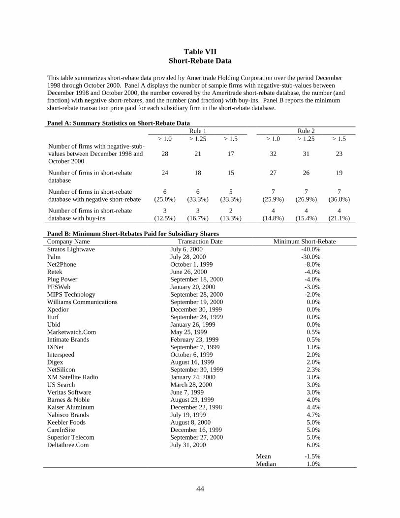
44

Table VIIShort-Rebate Data

This table summarizes short-rebate data provided by Ameritrade Holding Corporation over the period December1998 through October 2000. Panel A displays the number of sample firms with negative-stub-values betweenDecember 1998 and October 2000, the number covered by the Ameritrade short-rebate database, the number (andfraction) with negative short-rebates, and the number (and fraction) with buy-ins. Panel B reports the minimumshort-rebate transaction price paid for each subsidiary firm in the short-rebate database.

Panel A: Summary Statistics on Short-Rebate DataRule 1 Rule 2

> 1.0 > 1.25 > 1.5 > 1.0 > 1.25 > 1.5Number of firms with negative-stub-values between December 1998 andOctober 2000

28 21 17 32 31 23

Number of firms in short-rebatedatabase

24 18 15 27 26 19

Number of firms in short-rebatedatabase with negative short-rebate

6(25.0%)

6(33.3%)

5(33.3%)

7(25.9%)

7(26.9%)

7(36.8%)

Number of firms in short-rebatedatabase with buy-ins

3(12.5%)

3(16.7%)

2(13.3%)

4(14.8%)

4(15.4%)

4(21.1%)

Panel B: Minimum Short-Rebates Paid for Subsidiary SharesCompany Name Transaction Date Minimum Short-RebateStratos Lightwave July 6, 2000 -40.0%Palm July 28, 2000 -30.0%Net2Phone October 1, 1999 -8.0%Retek June 26, 2000 -4.0%Plug Power September 18, 2000 -4.0%PFSWeb January 20, 2000 -3.0%MIPS Technology September 28, 2000 -2.0%Williams Communications September 19, 2000 0.0%Xpedior December 30, 1999 0.0%Iturf September 24, 1999 0.0%Ubid January 26, 1999 0.0%Marketwatch.Com May 25, 1999 0.5%Intimate Brands February 23, 1999 0.5%IXNet September 7, 1999 1.0%Interspeed October 6, 1999 2.0%Digex August 16, 1999 2.0%NetSilicon September 30, 1999 2.3%XM Satellite Radio January 24, 2000 3.0%US Search March 28, 2000 3.0%Veritas Software June 7, 1999 3.0%Barnes & Noble August 23, 1999 4.0%Kaiser Aluminum December 22, 1998 4.4%Nabisco Brands July 19, 1999 4.7%Keebler Foods August 8, 2000 5.0%CareInSite December 16, 1999 5.0%Superior Telecom September 27, 2000 5.0%Deltathree.Com July 31, 2000 6.0%

Mean -1.5%Median 1.0%

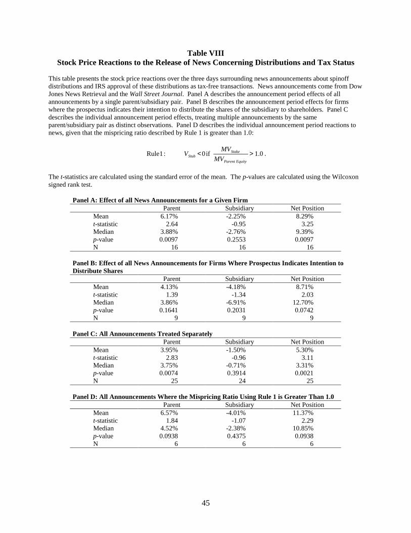
45

Table VIIIStock Price Reactions to the Release of News Concerning Distributions and Tax Status

This table presents the stock price reactions over the three days surrounding news announcements about spinoffdistributions and IRS approval of these distributions as tax-free transactions. News announcements come from DowJones News Retrieval and the Wall Street Journal. Panel A describes the announcement period effects of allannouncements by a single parent/subsidiary pair. Panel B describes the announcement period effects for firmswhere the prospectus indicates their intention to distribute the shares of the subsidiary to shareholders. Panel Cdescribes the individual announcement period effects, treating multiple announcements by the sameparent/subsidiary pair as distinct observations. Panel D describes the individual announcement period reactions tonews, given that the mispricing ratio described by Rule 1 is greater than 1.0:

0.1if0:1Rule

><EquityParent

StakeStub MV

MVV .

The t-statistics are calculated using the standard error of the mean. The p-values are calculated using the Wilcoxonsigned rank test.

Panel A: Effect of all News Announcements for a Given FirmParent Subsidiary Net Position

Mean 6.17% -2.25% 8.29%t-statistic 2.64 -0.95 3.25Median 3.88% -2.76% 9.39%p-value 0.0097 0.2553 0.0097N 16 16 16

Panel B: Effect of all News Announcements for Firms Where Prospectus Indicates Intention toDistribute Shares

Parent Subsidiary Net PositionMean 4.13% -4.18% 8.71%t-statistic 1.39 -1.34 2.03Median 3.86% -6.91% 12.70%p-value 0.1641 0.2031 0.0742N 9 9 9

Panel C: All Announcements Treated SeparatelyParent Subsidiary Net Position

Mean 3.95% -1.50% 5.30%t-statistic 2.83 -0.96 3.11Median 3.75% -0.71% 3.31%p-value 0.0074 0.3914 0.0021N 25 24 25

Panel D: All Announcements Where the Mispricing Ratio Using Rule 1 is Greater Than 1.0Parent Subsidiary Net Position

Mean 6.57% -4.01% 11.37%t-statistic 1.84 -1.07 2.29Median 4.52% -2.38% 10.85%p-value 0.0938 0.4375 0.0938N 6 6 6