Embed Size (px)
Citation preview
Limit Theory for Spatial Processes, Bootstrap
Quantile Variance Estimators, and Efficiency
Measures for Markov Chain Monte Carlo
Xuan Yang
Submitted in partial fulfillment of the
requirements for the degree
of Doctor of Philosophy
in the Graduate School of Arts and Sciences
COLUMBIA UNIVERSITY
2014

c©2014
Xuan Yang
All Rights Reserved
ABSTRACT
Limit Theory for Spatial Processes, Bootstrap
Quantile Variance Estimators, and Efficiency
Measures for Markov Chain Monte Carlo
Xuan Yang
This thesis contains three topics: (I) limit theory for spatial processes, (II) asymptotic
results on the bootstrap quantile variance estimator for importance sampling, and
(III) an efficiency measure of MCMC.
(I) First, central limit theorems are obtained for sums of observations from a κ-
weakly dependent random field. In particular, it is considered that the observations
are made from a random field at irregularly spaced and possibly random locations.
The sums of these samples as well as sums of functions of pairs of the observations
are objects of interest; the latter has applications in covariance estimation, composite
likelihood estimation, etc. Moreover, examples of κ-weakly dependent random fields
are explored and a method for the evaluation of κ-coefficients is presented.
Next, statistical inference is considered for the stochastic heteroscedastic processes
(SHP) which generalize the stochastic volatility time series model to space. A com-

posite likelihood approach is adopted for parameter estimation, where the composite
likelihood function is formed by a weighted sum of pairwise log-likelihood functions.
In addition, the observations sites are assumed to distributed according to a spa-
tial point process. Sufficient conditions are provided for the maximum composite
likelihood estimator to be consistent and asymptotically normal.
(II) It is often difficult to provide an accurate estimation for the variance of the
weighted sample quantile. Its asymptotic approximation requires the value of the
density function which may be hard to evaluate in complex systems. To circumvent
this problem, the bootstrap estimator is considered. Theoretical results are estab-
lished for the exact convergence rate and asymptotic distributions of the bootstrap
variance estimators for quantiles of weighted empirical distributions. Under regular-
ity conditions, it is shown that the bootstrap variance estimator is asymptotically
normal and has relative standard deviation of order O(n−1/4).
(III) A new performance measure is proposed to evaluate the efficiency of Markov
chain Monte Carlo (MCMC) algorithms. More precisely, the large deviations rate of
the probability that the Monte Carlo estimator deviates from the true by a certain
distance is used as a measure of efficiency of a particular MCMC algorithm. Numerical
methods are proposed for the computation of the rate function based on samples of
the renewal cycles of the Markov chain. Furthermore the efficiency measure is applied
to an array of MCMC schemes to determine their optimal tuning parameters.

Contents
List of Tables v
List of Figures vi
Acknowledgments vii
Chapter 1 Introduction and Overview 1
Chapter 2 Central limit theorems for random fields and weak depen-
dence 6
2.1 Introduction . . . . . . . . . . . . . . . . . . . . . . . . . . . . . . . . 7
2.2 Central limit theorem for samples collected at fixed observation locations 9
2.2.1 Central limit theorem for partial sums . . . . . . . . . . . . . 9
2.2.2 Central limit theorem for Gn . . . . . . . . . . . . . . . . . . . 13
2.3 Central limit theorem for observations at random locations . . . . . . 15
2.4 Examples . . . . . . . . . . . . . . . . . . . . . . . . . . . . . . . . . 19
2.5 Proofs . . . . . . . . . . . . . . . . . . . . . . . . . . . . . . . . . . . 24
2.5.1 Proofs for results in Section 2.2 . . . . . . . . . . . . . . . . . 24
2.5.2 Proofs for results in Section 2.3 . . . . . . . . . . . . . . . . . 30
2.5.3 Proofs for results in Section 2.4 . . . . . . . . . . . . . . . . . 36
i
2.6 A comparison of the notions of weak dependence . . . . . . . . . . . . 41
2.7 Weak dependence of spatial point processes . . . . . . . . . . . . . . 47
Chapter 3 Statistical inference for the stochastic heteroscedastic pro-
cess 52
3.1 Introduction . . . . . . . . . . . . . . . . . . . . . . . . . . . . . . . . 53
3.2 Stochastic volatility models in space and composite likelihood estimations 55
3.2.1 Stochastic heteroscedastic processes . . . . . . . . . . . . . . . 55
3.2.2 Estimations of the SHP model with the composite likelihood . 58
3.3 Consistency and Asymptotic Normality . . . . . . . . . . . . . . . . . 59
3.4 Computations and Empirical studies . . . . . . . . . . . . . . . . . . 64
3.4.1 Computations for the pairwise likelihood function . . . . . . . 64
3.4.2 Subsampling for variance estimations . . . . . . . . . . . . . . 65
3.4.3 Simulation study . . . . . . . . . . . . . . . . . . . . . . . . . 66
3.5 Proofs . . . . . . . . . . . . . . . . . . . . . . . . . . . . . . . . . . . 69
3.5.1 Properties of the pairwise likelihood function of SHP model . 69
3.5.2 Proofs for the main theorem . . . . . . . . . . . . . . . . . . . 71
3.5.3 Proof of Proposition 24 . . . . . . . . . . . . . . . . . . . . . . 75
3.5.4 Proof of Proposition 25 . . . . . . . . . . . . . . . . . . . . . . 76
3.5.5 κ-weak dependence of the SHP model . . . . . . . . . . . . . . 86
3.5.6 Proof of Proposition 26 . . . . . . . . . . . . . . . . . . . . . . 91
3.6 Moment estimations for µ and σ2 . . . . . . . . . . . . . . . . . . . . 97
3.7 Gauss-Hermite quadrature and numerical integration for Gaussian ran-
dom variables . . . . . . . . . . . . . . . . . . . . . . . . . . . . . . . 98
3.8 The score function of the bivariate Gaussian random variables . . . . 100
ii
Chapter 4 The Convergence Rate and Asymptotic Distribution of
Bootstrap Quantile Variance Estimator for Importance Sampling 101
4.1 Introduction . . . . . . . . . . . . . . . . . . . . . . . . . . . . . . . . 102
4.2 Main results . . . . . . . . . . . . . . . . . . . . . . . . . . . . . . . . 105
4.2.1 Problem setting . . . . . . . . . . . . . . . . . . . . . . . . . . 105
4.2.2 Related results . . . . . . . . . . . . . . . . . . . . . . . . . . 107
4.2.3 The results for regular quantiles . . . . . . . . . . . . . . . . . 108
4.2.4 Results for extreme quantile estimation . . . . . . . . . . . . . 111
4.3 A numerical example . . . . . . . . . . . . . . . . . . . . . . . . . . . 113
4.4 Proof of Theorem 41 . . . . . . . . . . . . . . . . . . . . . . . . . . . 115
4.5 Proof of Theorem 42 . . . . . . . . . . . . . . . . . . . . . . . . . . . 120
4.6 Proof of Theorem 43 . . . . . . . . . . . . . . . . . . . . . . . . . . . 134
Chapter 5 Evaluating the Efficiency of Markov Chain Monte Carlo
From a Large Deviations Point of View 141
5.1 Introduction . . . . . . . . . . . . . . . . . . . . . . . . . . . . . . . . 142
5.2 A Large Deviations Performance Measure of an MCMC Algorithm . . 145
5.2.1 MCMC and Numerical Integration . . . . . . . . . . . . . . . 145
5.2.2 Error Probabilities and Large Deviations . . . . . . . . . . . . 147
5.2.3 The Analytic Form of the Rate Function . . . . . . . . . . . . 150
5.3 Numerical Methods for Computing the Rate Function . . . . . . . . . 154
5.3.1 Computing the Rate Function by Simulation . . . . . . . . . . 155
5.3.2 Computing the Rate Function by the Discretization Method . 158
5.4 Numerical Results . . . . . . . . . . . . . . . . . . . . . . . . . . . . . 159
5.4.1 Gaussian Target Distribution . . . . . . . . . . . . . . . . . . 160
5.4.2 Laplace Target Distribution . . . . . . . . . . . . . . . . . . . 163
iii

5.4.3 A Bimodal Target Distribution . . . . . . . . . . . . . . . . . 165
5.4.4 Tuning the temperature for parallel tempering . . . . . . . . . 170
Bibliography 173
iv

List of Tables
3.1 Maximum composite likelihood estimations . . . . . . . . . . . . . . . 68
3.2 Subsampling estimations of standard deviations . . . . . . . . . . . . 68
4.1 Comparison of variance estimators for fixed m = 10 and n = 10, 000. . 113
4.2 Comparison of variance estimators as m → ∞, αp = 1.5m, and n =10, 000. . . . . . . . . . . . . . . . . . . . . . . . . . . . . . . . . . . . 114
v

List of Figures
3.1 Frequency plot of the MCLE . . . . . . . . . . . . . . . . . . . . . . . 67
3.2 A comparison between the MCLE and the MME . . . . . . . . . . . . 98
5.1 Gaussian proposals . . . . . . . . . . . . . . . . . . . . . . . . . . . . 162
5.2 Normal proposals . . . . . . . . . . . . . . . . . . . . . . . . . . . . . 164
5.3 Gaussian proposals vs. Laplace proposals. . . . . . . . . . . . . . . . 166
5.4 Regional adaptive proposals . . . . . . . . . . . . . . . . . . . . . . . 169
5.5 Parallel tempering . . . . . . . . . . . . . . . . . . . . . . . . . . . . 172
vi

Acknowledgments
I would like to use this opportunity to extend my sincere gratitude to my advisors
Professor Richard A. Davis and Professor Jingchen Liu, for their invaluable guidance
to me in my five years at Columbia. I started to work with Jingchen in the first
summer break. It was him introduced me into the research in applied probability. He
is also like a big brother to me that he has always been highly supportive through-
out my graduate years. Richard lead me to gain numerous insights into time series
analysis and spatial statistics. He is my role model in my academic life in pursuit
of deep knowledge and high standards of professional conduct. I feel really fortunate
to have the opportunity to work for both Richard and Jingchen. Their advices, en-
couragement, and inspirations shed on me will continue to benefit me in my future
career.
I would like to thank our collaborator Professor Henrik Hult, who taught me the
theory of large deviations in a PhD topic course when he visited Columbia in Fall
2010. I am grateful to Professor Zhiliang Ying, who is always willing to help when I
turn to him, and Professor Gongjun Xu, who has generously shared with me a lot of
his experiences when he was also a PhD student at Columbia. My thanks also go to
vii

many Columbia professors and visiting professors who give me inspirations and my
fellow students with whom we exchange ideas and share the fun in graduate life.
I would also like to thank Professors Jose H. Blanchet, Victor de la Pena, and
Mariana Olvera-Cravioto, who have generously agreed to sit on my defense committee
and provided we helpful feedbacks on my thesis.
Last but most importantly, I would like to thank my parents, for their love and
support.
viii

To My Parents
ix

1
Chapter 1
Introduction and Overview
This thesis can be grouped into topics: (I) limit theory for spatial processes, (II)
asymptotic results on the bootstrap quantile variance estimator for importance sam-
pling, and (III) an efficiency measure of MCMC.
The first part on limit theory for spatial processes is contained in Chapters 2 and
3. Chapter 2 establishes central limit theorems for sums of observations and pairs
of observations from random fields under general settings. Especially the observa-
tions sites are irregularly spaced and possibly random. Central limit theorems for
random fields play vital roles in statistical inference for spatial models. For example
the estimation of means and covariances for pairs of observations. Existing theories,
however, are not adequate in many applications. They often make stringent depen-
dence assumptions such as strong mixing or association which are difficult to verify.
Moreover, few of them are well adapted to irregularly spaced locations therefore they
don’t apply to the continuous domain case; see Doukhan (1995); Bradley (2005);
Gaetan and Guyon (2010); Bulinski and Shashkin (2007).
In our research we use the notion of κ-weak dependence due to Doukhan and
2
Louhichi (1999). In the literature, many weak dependence notions are proposed to
study moments and tail probabilities of partial sums of stochastic processes indexed
by Z. In a broad sense, the κ-weak dependence is one of the weaker dependence
conditions for establishing central limit theorems; see Dedecker et al. (2007) for a
comprehensive survey of notions of weak dependence. We adapt this framework for
random fields. In the asymptotic analysis, two scenarios of irregularly spaced obser-
vations sites are considered—deterministic locations and random locations, which in
the latter case, the sites are assumed to be distributed according to a spatial point
process. For each of these scenarios, we provide sufficient conditions under which
the sum of observations and the sum of functions of pairs are asymptotically normal
for increasing domain. In addition, to verify the weak dependence assumptions, we
provide a way to estimate the κ-coefficients in an array of spatial random fields and
point processes.
Chapter 3 concerns statistical inference for the stochastic heteroscedastic processes
(SHP). Although Gaussian models are commonly used in spatial statistics, they have
a number of drawbacks. First, Gaussian models may not be adequate to model certain
features of the data, such as heavy-tails and clustering of large values. Second the
predictors from Gaussian models are restricted. These predictors are linear functions
of the observed data and the predicted variances depend only on the observations
through their covariances but not on the actual value of the data. This indicates
that predictions in a region with large observed values have the same predicability
with those in a region with small observations. To overcome these limits, many non-
Gaussian models have been proposed, c.f. Steel and Fuentes (2010), and here we
consider the SHP model due to Palacios and Steel (2006) and Huang et al. (2011),
which incorporates a volatility component to capture the heterogeneity of variation
at different observations sites.

3
To estimate a SHP model, the usual maximum likelihood method is not feasible.
As the full likelihood is a multiple integral whose dimension equals the sample size, its
evaluation incurs a high computational cost. To bypass this limitation, a composite
likelihood approach has been considered for parameter estimation. It only involves
the calculation of low-dimensional likelihood functions and offers a more promising
solution for large data sets. Specifically, the composite likelihood takes the form
a weighted sum of pairwise likelihood functions, each of which can be efficiently
evaluated using the Gauss-Hermite quadrature. Sufficient conditions are provide so
that the maximum composite likelihood estimator is consistent and asymptotically
normal. These theoretical results are built upon the central limit theorems in Chapter
2. Additional effort is made to evaluate the κ-coefficients for the SHP model and to
derive moment bounds for the pairwise likelihood function.
Chapter 4 contains asymptotic results for the bootstrap quantile variance estima-
tor for importance sampling.1 Consider the problem of quantile estimation for small
or large probabilities, where p is close to 0 or 1. The computation for such quantiles
is often required in engineering and finance as they are measures of reliability and
risk. As the variance of the sample quantile estimator is proportional to the recipro-
cal of probability density function, the sample quantile becomes unstable when the
quantile probability is close to zero or one where the density function is usually small.
A common practice to reduce variance is through the use of importance sampling to
produce more samples near the quantile of interest and calculate the weighted sample
quantile estimator; see Glynn (1996).
The variance of the weighted sample quantile estimator is usually a difficult quan-
tity to compute. Its evaluation requires knowledge of the probability density function
1This work is first published in Advances in Applied Probability, Vol.44 No.3 c©2012 by TheApplied Probability Trust; see Liu and Yang (2012).
4
whose calculation is sometimes intractable in complex systems. In this study, we
consider the bootstrap estimator for the variance to avoid such computations. The
contributions of this study are threefold. First, sufficient conditions are provided for
the quantiles of weighted samples to have finite variances. The asymptotic approxi-
mations of this variance is also examined. Second, the asymptotic distribution of the
bootstrap estimator is derived. Under regularity conditions, we show that the boot-
strap variance estimator is asymptotically normal and has relative standard deviation
of order O(n−1/4). Such a result can be considered as a generalization of the one by
Hall and Martin (1988) for unweighted samples. Third we establish corresponding
results in the domain where large deviations hold.
Chapter 5 is on efficiency measure of MCMC algorithms. A crucial issue in the
study of MCMC is the evaluation of efficiency and the selection of an optimal transi-
tion probability usually within a parametric family. We try to address this problem
from a large deviations point of view. In the context of numerical integration, one is
interested in the calculation of an integral I =∫g(x)π(x)dx, where π is a probability
density function for which random samples are generated by an MCMC algorithm.
The empirical mean In = 1n
∑ni=1 g(Xi), forms an estimator of the integral I. We
consider the error probability P(In − I ∈ F ) for some error set F that is bounded
away from zero. We propose to use the large deviations rate of this error probability
to access the efficiency of different MCMC algorithms—a larger rate implies faster
decay of the error probability as the sample size increases and therefore the respective
algorithm is better.
Based on the pinned large deviations theory for irreducible Markov chains in
Ney and Nummelin (1987a,b), we develop numerical methods to evaluate the large
deviations rate and apply this efficiency measure to determine the optimal tuning
parameters for the transition probabilities. Furthermore, the optimal values of the

5
tuning parameters appear quite stable in numerical examples over different choices of
the error set F .

6
Chapter 2
Central limit theorems for random
fields and weak dependence

7
2.1 Introduction
Central limit theorems concerning sums of observations from random fields often play
a key role in statistical inference of spatial models. Various notions such as mixing and
association, which characterize dependence structures, drive the asymptotics in these
theorems. But there is a gap between the existing theoretical results and their statis-
tical applications, which is mainly due to the fact that the dependence assumptions
are often not easy to check and may even fail to hold in simple examples.
In this chapter we develop central limit theorems under conditions on the κ-
coefficients and provide ways to estimate them in various spatial models. The κ-
coefficients and the notion of κ-weak dependence was first introduced in Doukhan
and Louhichi (1999) in the context of time series and they are tools for obtaining
bounds on the moments and tail probabilities of the sums of observations. In a broad
sense, the κ-coefficients are relatively easier to evaluate and less stringent than the
common mixing coefficients; See Dedecker et al. (2007) for a comprehensive survey of
weak dependence. We adapt their framework for the study of spatial random fields.
We first consider the sum of observations at irregularly spaced locations for a
random field and provide sufficient conditions under which the sum converges in
distribution to a normal for increasing domain asymptotics. The weak dependence
condition is formulated in turns of decay of the κ-coefficients. Moreover we allow
the random field to be non-stationary and we make very general assumptions on the
configuration of observation sites so that the result is readily to be applied in a wide
spectrum of situations.
Then we extend such result for sums of functions of pairs, which has applications in
covariance estimation and composite likelihood estimation. For instance, consider the
parameter estimation when the full likelihood function is intractable, one can instead
8
use a composite likelihood function which could be a weighted sum of pairwise log-
likelihood functions. We propose a framework to deal with such double sums, which
is possible to be extend to sums of functions of q-tuples.
Next, we consider random observation sites and establish parallel asymptotic re-
sults for sums of observations and sums of functions of pairs. In particular, the
observations sites are determined by a spatial point process that is independent of
the random field. Such a structure provides a natural way to integrate the selection of
observations sites into modeling and capture the irregularity pattern that may present
in observations locations. In the development of our results, we generalize the notion
of κ-coefficients and apply it to point processes.
At last, to provide ways to verify the weak dependence assumptions, we inves-
tigate the κ-coefficients in various spatial random fields and point processes. The
κ-coefficients for Gaussian random fields have explicit forms. For more general mod-
els, we introduce a technique to construct upper bounds for the κ-coefficients and
apply it in an array of examples including max-stable processes, shot noise processes,
Cox processes and etc.
Central limit theorems for sums of observations from random fields has been con-
sidered by many authors. Most previous results are restricted to random fields on
a regular lattice and strong mixing assumptions. Among them, Bolthausen (1982)
is the first to prove a central limit theorem for a stationary random field on Zm
under conditions on the decay of the α-mixing coefficients. In the same spirit, Jen-
ish and Prucha (2009, 2012) extend the results to triangular arrays of random fields
observed on a regular lattice; Lahiri (2003) considers central limit theorems with a
spatial sampling design according to a fixed i.i.d sequence and a scale parameter. For
variants of central limit theorems with different types of mixing coefficients, one can
refer to Doukhan (1995) and Bradley (2005). Another important type of dependence
9
conditions relates to the notion of association and central limit theorems are also
established for associated random fields, see Bulinski and Shashkin (2007) for details.
The rest of the chapter is organized as follows. Section 2.2 contains the central lim-
it theorems with observations made at fix locations. The parallel results for random
locations are established in Section 2.3. In Section 2.4, we explore various examples of
random fields and spatial point processes and evaluate their κ-coefficients. To avoid
deterring the flow of this chapter, proofs of all theorems, propositions and lemmas
are deferred to Section 2.5.
2.2 Central limit theorem for samples collected at
fixed observation locations
2.2.1 Central limit theorem for partial sums
Throughout this chapter we consider a real-valued random field indexed by elements
in a topological space S, denoted by Y (s); s ∈ S. The topological space S is
endowed with a distance function d satisfying d(s1, s2) = d(s2, s1) and d(s1, s2) ≥ 0
for all s1, s2 ∈ S. The triangle inequality is not required. Moreover the process
Y is not necessarily stationary. Suppose Y is observed on a countable subset D =
s1, s2, ... ⊂ S. Furthermore, we define a monotone increasing sequence of domains
Sn ↑ S in which we observe the process Y . That is, we observe Y on the increasing
sequence of sets Dn = D ∩ Sn. One may consider that Sn is our sampling domain
where data are collected. Without loss of generality, the index n will correspond to
the cardinality of the set Dn, i.e., it is the sample size of the observed data. Naturally,
the sequence Dn is monotonely increasing to D. Of interest in this chapter are the
10
asymptotic behavior of the summation
Sn =∑s∈Dn
Y (s) (Q1)
and the double summation
Gn =∑
s1 6=s2∈Dn
gs1,s2(Y (s1), Y (s2)), (Q2)
where g is a real-valued function of locations s1, s2 and values of Y (s1), Y (s2). We
will establish sufficient and checkable conditions under which Sn and Gn are asymp-
totically normal.
The statements of the conditions involve the following construction, which is based,
to a large extent, on the development of weak dependence of Doukhan and Louhichi
(1999) and Dedecker et al. (2007). Let U and V be finite subsets of S. Define the
distance between two sets as d(U, V ) = infd(s, s′); s ∈ U, s′ ∈ V and
κY (U, V ) = sup0<Lip(h1),Lip(h2)<∞
|Cov(h1(YU), h2(YV ))||U ||V |Lip(h1)Lip(h2)
,
where YU = (Y (s); s ∈ U) is a vector, |U | and |V | denote the cardinality of the
respective sets, and h1 : RI → R, h2 : RJ → R are Lipschitz functions with coefficient
Lip(hj)4= sup
x,y
|hj(x)− hj(y)|∑i |x(i) − y(i)|
, j = 1, 2,
in which x(i) denotes the ith coordinates of x. The κ-coefficient for process Y is
defined as
κY (l1, l2, r) = supκY (U, V ); |U | ≤ l1, |V | ≤ l2, d(U, V ) ≥ r, (2.1)
whereas l1, l2 are positive integers and r ≥ 0. It is straightforward by the definition
that κY (l1, l2, r) is non-decreasing as l1 or l2 increases and it is non-increasing as

11
r increases. Furthermore, we define κY (l1,∞, r) = supl2 κY (l1, l2, r) and κY (r) =
supl1,l2 κY (l1, l2, r). When the random field is uniformly bounded in L2 norm, the
κ-coefficients are always finite.
Proposition 1 κY (0) = supVarY (s); s ∈ S.
Definition 1 A random field Y (s); s ∈ S is said to be κ-weakly dependent if
limr→∞ κY (r) = 0.
Now we present a list of conditions for the central limit theorem of Sn.
Assumption 1 The set D is deterministic. For each j = 1, 2, ..., define
rj = supr : sups∈D|s′ ∈ D; d(s, s′) < r| ≤ j − 1,
i.e. rj is the radius at which all balls of radius less than rj centered at s ∈ D, has at
most j − 1 points in D. Assume limj→∞ rj =∞.
Assumption 2 Second order uniform integrability: limM→∞ sups∈S E[Y 2(s); |Y (s)| ≥
M ] = 0.
Assumption 3 The κ-coefficients of the random field Y satisfy:∑∞j=1 κY (2, 2, rj) <∞ and κY (1,∞, rj) = o(j−2).
Assumption 4 Let σ2n = Var(Sn) and then lim infn→∞ σ
2n/n > 0.
Assumption 5 EY (s) = 0.
Theorem 2 Under Assumptions 1-5, Sn/σn converges in distribution to N (0, 1) as
n→∞.
12
The most relevant work to the current one is given by Dedecker et al. (2007) who
develop central limit theorem for uniformly bounded κ-weakly dependent random
fields observed on the regular lattice D = Zm. Furthermore, the central limit theorem
based on α-mixing coefficients and near-epoch dependence is developed by Jenish and
Prucha (2009, 2012). These papers constrain the minimum distance of any pair of
observation locations to be greater than 0. Theorem 2 is a generalization of these
results from the following perspectives: Our results fit general irregular lattice which
can have local clusters of finite size whose members are arbitrarily close; We use less
restrictive weak dependence assumptions that based on the κ-coefficients.
In particular, Assumption 1 allows elements in D to be arbitrarily close. For
example, if for some small j, rj = 0, then for any s ∈ D, there could be j element
in D that are arbitrarily close to s. Nonetheless, it does exclude the existence of
accumulation points in D in any local region. Since there exists some ri > 0, there
won’t be more than i observations in any open ball with radius less than ri.
Assumption 2 is the L2 uniform integrability of the random field. A similar con-
dition is required by Jenish and Prucha (2009, 2012). Technically speaking, it allows
one to localize Y to a bounded region. It also implies sups∈S E(Y 2(s)) < ∞. As-
sumption 3 concerning the decaying rate of the κ-coefficients is comparable to those
for the α-mixing coefficients imposed in Bolthausen (1982); Guyon (1995); Jenish and
Prucha (2009, 2012). A sufficient for Assumption 3 is κY (rj) = o(j−2), which we will
provide ways to verify in a latter section.
Theorem 2 does not require stationarity of the random field. Instead we employ
Assumption 4, which, together with the second order uniform integrability (Assump-
tion 2), ensure that sups∈S EY 2(s)/σ2n → 0 as n → ∞. Recall the Lindeberg
condition in the central limit theorem for independent but non-identically distributed
random variables, which implies that supi Var(Yi)/σ2n → 0 as n → ∞. A sufficient
13
condition for Assumption 4 is infs∈S EY 2(s) > 0 and Cov(Y (s), Y (s′)) ≥ 0 for any
s, s′ ∈ S.
2.2.2 Central limit theorem for Gn
We now proceed to the central limit theorem for Gn that arises from the anal-
ysis of estimating equations of spatial models. The main idea there is to view
gs1,s2(Y (s1), Y (s2)) : s1, s2 ∈ S as a random field living on the product space
S × S so that the double sum can be treated in a similar way to the single sum.
Before we illustrate our result, there are two things worth to be mentioned. First,
the pair observation sites (si, sj) now form a grid-like structure and increasing of sam-
ple size has a different impact on the double sum compared with the single sum. The
generality we made for the index space S and observation sitesD now pays off. We can
use similar analysis for the double sum as the single sum without worrying to much
about the effect of pair sites. Second, pair observation can potentially lead to high-
er dependence in the summand of the double sum. For example gs1,s2(Y (s1), Y (s2))
maybe highly correlated with gs1,sn(Y (s1), Y (sn)) no matter how large n is. This
prompt us to restrict the form of g. In our development, we assume g is band-limited
in the following sense.
Assumption 6 There exists cg > 0 such that, gs1,s2(x, y) = 0 for all d(s1, s2) > cg
and x, y ∈ R.
We can define the κ-coefficients for the process gs1,s2(Y (s1), Y (s2)) : s1, s2 ∈ S.
First, the distance between any two points (s1, s2) and (t1, t2) in S × S is defined as
d∗ ((s1, s2), (t1, t2)) = mind(si, tj) : i = 1, 2, j = 1, 2,
14
which is non-negative and symmetric. Note that d∗ is typically not a metric since it
does not satisfy the triangle inequality. Then cponsider two subsets U, V ⊂ S × S.
Let d∗(U, V ) = mind∗(s1, t2) : s1 ∈ U, s2 ∈ V . For some finite subset of U ⊂ S ×S,
let
gU(Y ) = (gs1,s2(Y (s1), Y (s2)) : (s1, s2) ∈ U) ,
denote the finite dimensional random vector on U and
κg(U, V ) = sup0<Lip(h1),Lip(h2)<∞
|Cov (h1(gU(Y )), h2(gV (Y ))) ||U ||V |Lip(h1)Lip(h2)
.
The κ-coefficient for the pair process gs1,s2(Y (s1), Y (s2)) : s1, s2 ∈ S is defined as
κg(l1, l2, r) = supκg(U, V ) : U, V ⊂ S × S, |U | ≤ l1, |V | ≤ l2, d∗(U, V ) ≥ r (2.2)
where l1 and l2 are positive integers and r ≥ 0. We now provide a list of conditions
for the central limit theorem of Gn.
Assumption 7 Second order uniform integrability:
limM→∞
sups1,s2∈S
E[g2s1,s2
(Y (s1), Y (s2)); |gs1,s2(Y (s1), Y (s2))| > M ] = 0.
Assumption 8 The κ-coefficients satisfy:∑∞
j=1 κg(2, 2, rj) <∞ and κg(1,∞, rj) =
o(j−2).
Assumption 9 lim infn→∞Var(Gn)/n > 0.
Theorem 3 Under Assumptions 1 and 6-9, Gn − E(Gn)/√
Var(Gn) converges in
distribution to N (0, 1) as n→∞.
15
2.3 Central limit theorem for observations at ran-
dom locations
In this section, we consider the situation when observations are made at random
locations, that is, the collection of observation sites, D is now generated by a point
process living on S, which the point process is denoted by
N(·) =∑s∈D
δs(·)
where δs is the point mass at location s. For simplicity, we further restrict the analysis
to S = Rm.
We consider the point process N to be a general Poisson point process with inten-
sity measure λ, which is not necessarily homogeneous. But the results developed in
this section can be extended to more general point processes such as the Cox process-
es and the Poisson cluster processes; see Baddeley (2006) for general point processes.
Under the random sampling of locations, the single sum (Q1) and double sum (Q2)
now can be represented in terms of integrals
Sn =
∫SnY (s)N(ds), (Q1’)
Gn =
∫Sn
∫Sngs1,s2(Y (s1), Y (s2))N[2](ds1, ds2), (Q2’)
where N[2](ds1, ds2) = N(ds1)N(ds2)Is1 6=s2. In order that above the integrals are well
defined, Y is assumed to have Borel measurable sample paths and g, as a function of
(s1, s2, Y (s1), Y (s2)), is assumed to be Borel measurable. We use Q(s, r) = ×mi=1[s(i)−r2, s(i) + r
2) to denote the m-dimensional cube centered around s = (s(1), · · · , s(m)) ∈
Rm with length r ≥ 0 and Q(s, r) = ×mi=1[s(i)− r2, s(i) + r
2]. Let µ denote the Lebesgue
measure on Rm.

16
Based on the above setup, we list a set of technical conditions and the asymp-
totic results. Assumption 15 is a regularity condition for increasing domain, see also
Bolthausen (1982) and Bulinski and Shashkin (2007). Assumption 11 is on the weak
dependence of random field Y . Assumption 12 ensures that the limit distribution
under consideration does not degenerate. The same as before, stationarity is not
assumed for either the random field Y or the point process N .
Assumption 10 Define D∗n = s ∈ Zm;Q(s, 1) ∩ Sn 6= ∅, Dn = s ∈ Zm;Q(s, 1) ⊂
Sn and then
|Dn| → ∞,|Dn||D∗n|
→ 1, as n→∞.
Assumption 11 The κ-coefficients of Y (s); s ∈ Rm satisfy∑∞
j=0(j+1)m−1κY (2, 2, j) <
∞ and κY (1,∞, r) = o(r−2m).
Assumption 12 lim infn→∞Var(Sn)/µ(Sn) > 0.
Theorem 4 If the Poisson process N is independent of Y and sups∈Rm EN(Q(s, 1))4 <
∞, then under Assumption 2, 15–12, Sn−ESn√VarSn
converges in distribution to N (0, 1) as
n→∞.
Moreover we also provide results for the double sum Gn under the random sam-
pling of locations. Assumptions 13 and 14 are similar to Assumptions 8 and 9, but
the current assumptions are adapted for a random location setup.
Assumption 13 The κ-coefficients of gs1,s2(Y (s1), Y (s2)); s1, s2 ∈ Rm satisfy:∑∞j=0(j + 1)m−1κg(2, 2, j) <∞ and κg(1,∞, r) = o(r−2m).
Assumption 14 lim infn→∞Var(Gn)/µ(Sn) > 0.

17
Theorem 5 If the Poisson process N is independent of Y and sups∈Rm EN(Q(s, 1))8 <
∞, then under Assumptions 6, 7, 15, 13–14, Gn − E(Gn)/√
VarGn converges in
distribution to N (0, 1) as n→∞.
Remark 1 If Y and N are both stationary and function g is symmetric and transla-
tion invariant in the sense that gs1,s2(y1, y2) = g0,s2−s1(y1, y2) = gs2−s1,0(y2, y1) for any
s1, s2 ∈ Rm, y1, y2 ∈ R, let λ(ds) = λ0ds, then we have limn→∞1
µ(Sn)Var(Gn) = σ2
G,
where
σ2G =
∫Q(0,1)×(Rm)3
Cov (gs1,s2(Y (s1), Y (s2)), gs3,s4(Y (s3), Y (s4))) E(N[2](ds1, ds2)N[2](ds3, ds4)
),
=λ40
∫Q(0,1)×(Rm)3
Cov (gs1,s2(Y (s1), Y (s2)), gs3,s4(Y (s3), Y (s4))) ds1ds2ds3ds4
+ 4λ30
∫Q(0,1)×(Rm)3
Cov (gs1,s2(Y (s1), Y (s2)), gs1,s4(Y (s1), Y (s4))) ds1ds2ds4
+ 2λ20
∫Q(0,1)×(Rm)3
Var (gs1,s2(Y (s1), Y (s2))) ds1ds2
so that Assumption 14 can be removed in this case.
Theorem 4 and Theorem 5 can also be extended for more general point processes
N . Then the dependence structure of N weighs in our analysis, as evidenced from
the following decomposition
Var(Sn) = EVar(Sn|N)+ VarE(Sn|N),
which Var(Sn|N) in the first component is associated with Y and the second compo-
nent will rely on N .
We can adapt the notion of the κ-coefficients for N as well. For any set A ∈ B(Rm)
and Borel measurable function f : Rm → R bounded on A, let
NA(f) =
∫A
f(s)N(ds).
18
Let Q = Q(s, 1) : s ∈ Zm be the collection of all unit cubes with centers on
Zm. Then NA(f);A ∈ Q can be viewed as a random field on Zm, therefore the
κ-coefficients for N can be defined.
Definition 2 The first kind of κ-coefficient for N is defined for each l1, l2 ∈ N and
r ≥ 0 as
κN(l1, l2, r) = supCovh1 (NAi(f1), 1 ≤ i ≤ I) , h2
(NBj(f2), 1 ≤ j ≤ J
)
IJLip(h1)Lip(h2)‖f1‖∞‖f2‖∞,
where the supremum is taken over all unit cubes Ai, Bj ∈ Q, that d(Ai, Bj) ≥ r, 1 ≤
i ≤ I ≤ l1, 1 ≤ j ≤ J ≤ l2, 0 < Lip(h1),Lip(h2) < ∞ and 0 < ‖f1‖∞, ‖f2‖∞ < ∞,
in which ‖ · ‖∞ denotes the supreme norm of a function.
Definition 3 The second kind of κ-coefficient for N is defined for each r ≥ 0 as
κ∗N(r) = sup 1
‖f‖4∞
CovNA1(f)NA2(f), NB1(f)NB2(f), 1
‖f‖3∞
CovNA1(f)NA2(f), NB1(f)
where the supremum is taken over all unit cubes Ai, Bj ∈ Q, that d(Ai, Bj) ≥ r,
1 ≤ i ≤ 2, 1 ≤ j ≤ 2 and 0 < ‖f‖∞ <∞.
Note that the definition of κ∗N is not a special case of the definition of κN since
the product function NA1(f)NA2(f) is not Lipshitz in NA1(f) or NA2(f). For κ∗N , it is
used as a upper bound for the covariance of products of functionals NA(f). A similar
object is referred to as Cr,4 in Dedecker et al. (2007). Similarly we can also define the
κ-coefficients for N[2].
Then for Theorem 4 under the same conditions, if N is a point process satisfying
κN(1,∞, r) = o(r−2m), and∑∞
j=0(j + 1)m−1κ∗N(j) <∞, the conclusion of Theorem 4
still holds. Here the weak dependence condition for N is very similar to those for Y .
Theorem 5 can be extend in a similar way.
19
2.4 Examples
In this section, we evaluate the κ-coefficients for an array of random fields and point
processes. We propose strategies to obtain upper bounds for the κ-coefficients, which
in turn provide verification of the respective technical conditions on the decay of
κ-coefficients. These techniques are applied to a variety of processes, including Gaus-
sian, max-stable, shot noise, Neyman-Scott, and Cox processes.
2.4.0.0.1 Gaussian random fields. Consider a Gaussian process Y on Rm. By
a result of Shashkin (2002), the κ-coefficients of any Gaussian random field can be
computed explicitly by its covariance function
κY (l1, l2, r) = sups,t∈Rm,‖s−t‖≥r
|Cov(Y (s), Y (t))|, l1, l2 ∈ Z+, r ≥ 0, (2.3)
see also Doukhan and Louhichi (1999). Hence the κ-dependence is easy to check for
Gaussian processes. This is in contrast in contrast to the difficulties in verifying strong
mixing. The following example shows that a weakly dependent Gaussian random field
may not be strong mixing.
Example 1 Suppose Y is a stationary and isotropic Gaussian random field on Rm
with zero mean. Let C(h) = Cov(Y (s), Y (s + h)) denote the covariance function.
If C(h) is an analytic function, then the sample paths of Y are analytic; see Stein
(1999), Section 2.7. Consequently the σ-field of Y is generated through Y on any
dense set in any small open ball. Therefore αY (1,∞, r) = 14
for any r > 0 which
implies Y is not α-mixing. In particular, the common Gaussian covariance function
e−τ‖h‖2
and 1(a2+‖h‖2)1+τ
are analytic functions. On the other hand from (34), we see
that Y is κ-weakly dependent.
20
2.4.0.0.2 A technique to bound κ-coefficients. We now proceed to more com-
plicated processes for which direction calculation of κ-coefficients may not be feasible.
We introduce the concept of D-decomposition and use is to derive upper bounds for
the κ-coefficients.
Definition 4 For a random field Y on Rm, an additive decomposition
Y (s) = Y 〈r〉(s) + Y 〈r〉(s), s ∈ Rm (2.4)
is said to be a D-decomposition at distance r ≥ 0 if the process Y 〈r〉 is r-dependent,
that is, for any finite sets U, V ⊂ Rm such that d(U, V ) ≥ r, the vectors (Y 〈r〉(s); s ∈
U) and (Y 〈r〉(s′), s′ ∈ V ) are independent.
Definition 5 If Y has a D-decomposition for each r ≥ 0 and there exists a function
η : [0,∞)→ R such that
sups∈Rm
E |Y 〈r〉(s)|p ≤ η(r), r ≥ 0
for some p ≥ 2, then Y is said to have D-decompositions with Lp rate bounded by
η(r).
The D-decomposition splits the process into Y 〈r〉 that shows independence when
r distance apart and a residual process Y 〈r〉 whose pth moment is controlled by η(r).
The following proposition provides a bound for the κ-coefficient based on the above
decomposition.
Proposition 6 If Y has D-decompositions with L2 rate bounded by η(r) and sups∈Rm EY 2(s) =
M2 <∞, then κY (r) ≤ 3M12
2 η12 (r).
The following proposition constructs D-decompositions for Gaussian processes. It
relies on a kernel representation of the covariance functions and the D-decomposition
is obtained through a truncation on the associated kernel function.
21
Proposition 7 Suppose Y (s) is a Gaussian random field on Rm and its covariance
function admits the following kernel representation,
Cov (Y (s1), Y (s2)) =
∫kY (s1, s)kY (s2, s)ds. (2.5)
where kY : Rm × Rm → R is a Borel measurable function. Then for any r ≥ 0, Y (s)
has a D-decomposition where both Y 〈r〉 and Y 〈r〉 is are Gaussian random fields and
E Y 〈r〉(0) = 0. Furthermore, for any p ≥ 2, the Lp rate of these decompositions is
bounded by E |Z|pηp/2(r) where
η(r) = sups∈Rm
∫‖s′‖≥ r
2
k2Y (s, s− s′)ds′, (2.6)
and Z is a standard normal random variable. Hence κY (r) ≤ 3√
sups VarY (s)η 12 (r).
2.4.0.0.3 Max-stable processes. We consider a max-stable process Y with Frechet(p)
margins, p > 2. Where Frechet(p) denotes distribution with cumulative distribution
function e−x−pI(x > 0). According to the representation theory of max-stable pro-
cesses, c.f. de Haan and Ferreira (2006) and Resnick (2007), Y admits the following
form
Y (s) = max1≤i≤∞
ζiVi(s), s ∈ Rm (2.7)
where ζi; i ∈ N are the points of a Poisson point process on (0,∞] with intensity
ζ−1−pdζ and Vi are i.i.d copies of a non-negative continuous stochastic process V such
that EV p(s) = 1 for every s ∈ Rm.
Proposition 8 Let Y be a max-stable process with marginal distribution Frechet(p),
p > 2, as given in (2.7). Suppose that V has a D-decomposition with Lp rate bounded
by η(r). Then, Y has a D-decomposition with L2 rate bounded by 2Cη2p (r), where C
is the second moment of Frechet(p) and hence κY (r) ≤ 3√
2Cη1p (r).
22
One may consider constructing a max-stable process from some simple process
V , such as a Gaussian process, whose D-decomposition is available and therefore the
κ-coefficients of Y can be controlled.
2.4.0.0.4 Shot noise processes. Let NP be a stationary Poisson point process
NP on Rm with constant intensity λ0. A shot noise process is defined as
Y (s) =∑si∈NP
ξiφ(si − s), (2.8)
where ξi is a sequence of i.i.d random variables with finite second moments and φ
is a deterministic continuous function on Rm such that∫Rm|φ(s)|ds <∞,
∫Rm
φ(s)ds = 1,
∫Rm
φ2(s)ds <∞.
One can also write (2.8) as a stochastic intergral,
Y (s) =
∫Rm
ξs′φ(s′ − s)NP (ds′).
It is straightforward to verify that Y defined in (2.8) is stationary and
EY (s) = λ0 E(ξ), Cov (Y (s1), Y (s2)) = λ0 E(ξ2)
∫Rm
φ (s′ − s1)φ (s′ − s2) ds′.
We are particularly interested in the shot noise process because it constitutes
the intensity field of a large class of Neyman-Scott process, or more broadly Poisson
cluster processes, c.f. Møller (2003). To construct D-decompositions for the respective
point processes, we can utilize the D-decompositions of the shot noise processes. The
following proposition provides an upper bound of the κ-coefficient of Y (s).
Proposition 9 For each r ≥ 0, Y defined as in (2.8) has a D-decomposition
Y 〈r〉(s) =
∫Rm
ξs′φ〈r〉(s′ − s)NP (ds′) + λ0 E ξ
∫‖s′‖>r/2
φ(s′)ds′,
Y 〈r〉(s) =
∫Rm
ξs′φ〈r〉(s′ − s)NP (ds′)− λ0 E ξ
∫‖s′‖>r/2
φ(s′)ds′,
23
where φ〈r〉(s) = φ(s)I‖s‖≤r/2 and φ〈r〉(s) = φ(s)− φ〈r〉(s). Further it follows that there
exists some c1, c2 > 0 such that for all s ∈ Rm
EY 〈r〉(s)2 =λ0 E(ξ2)
∫‖s′‖> r
2
φ2(s′)ds′,
E |Y 〈r〉(s)|p ≤c1
(∫‖s′‖> r
2
|φ(s′)|pds′ +[ ∫‖s′‖> r
2
|φ(s′)|ds′]p)
,
and
κY (r) ≤ c2
(∫‖s′‖> r
2
φ2(s′)ds′) 1
2.
2.4.0.0.5 The process gs1,s2(Y (s1), Y (s2)). Recall that the analysis of Gn re-
quires bounds of the κ-coefficients of the process gs1,s2(Y (s1), Y (s2)). The following
proposition provides, for example, a bound when gs1,s2(y1, y2) is the log-likelihood
function of a Gaussian random field, that is, gs1,s2(y1, y2) is a degree-two polynomial
of x and y.
Proposition 10 Suppose Y (s); s ∈ Rm is a random field with sups∈Rm E |Y (s)|4 <
∞ and it has D-decompositions with L4 rate bounded by η. Let
gs1,s2(y1, y2) = [a(s1 − s2)y21 + b(s1 − s2)y1y2 + c(s1 − s2)y2
2]1|s1−s2|<cg ,
where a(x), b(x), and c(x) are uniformly bounded measurable functions on Rm. Then
the κ-coefficient of gs2,s1(Y (s1), Y (s2)) satisfies κg(r) = O(η14 (r)).
Under some regularity conditions, the above results can be further generalized
to other g-functions, although the analysis can be more tedious. Therefore we only
consider this simple case.
24
2.5 Proofs
2.5.1 Proofs for results in Section 2.2
The following lemma is used often to estimate the κ-coefficients.
Lemma 11 Let Xi, X′i, Zj, Z
′j, 1 ≤ i ≤ I, 1 ≤ j ≤ J , I, J ∈ Z+ be random variables
with finite 2nd moments, and h1, h2 are Lipschitz functions on RI and RJ respectively.
The following inequality holds
|Cov(h1(Xi, 1 ≤ i ≤ I)− h1(X ′i, 1 ≤ i ≤ I), h2(Zj, 1 ≤ j ≤ J)− h2(Z ′j, 1 ≤ j ≤ J)
)|
≤IJLip(h1)Lip(h2) sup1≤i≤I
‖Xi −X ′i‖2 sup1≤j≤J
‖Zj − Z ′j‖2
where ‖X‖24= (EX2)
12 In particular, by taking Z ′j = EZj, 1 ≤ j ≤ J , it immediately
follows that
|Cov (h1(Xi, 1 ≤ i ≤ I)− h1(X ′i, 1 ≤ i ≤ I), h2(Zj, 1 ≤ j ≤ J)) |
≤IJLip(h1)Lip(h2) sup1≤i≤I
‖Xi −X ′i‖2 sup1≤j≤J
(VarZj)12
Proof of Lemma 36. Since
‖h1(Xi, 1 ≤ i ≤ I)− h1(X ′i, 1 ≤ i ≤ I)‖2
≤∥∥Lip(h1)
I∑i=1
|Xi −X ′i|∥∥
2≤ Lip(h1)
I∑i=1
‖Xi −X ′i‖2
≤ILip(h1) sup1≤i≤I
‖Xi −X ′i‖2
and similarly∥∥h2(Zj, 1 ≤ j ≤ J)− h2(Z ′j, 1 ≤ j ≤ J)∥∥
2≤ JLip(h2) sup
1≤j≤J‖Zj − Z ′j‖2
Combining the above two inequalities, with Cauchy’s inequality we conclude the
lemma follows.
25
Proof of Proposition 1. For any finite sets U, V ⊂ S, and Lipshitz functions h1
and h2, using Lemma 36, it follows that
Cov (h1(YU), h2(YV )) ≤ Lip(h1)Lip(h2)|U ||V | sups∈U∪V
VarY (s).
So that κY (0) ≤ supVarY (s); s ∈ S. Further take U = V = s, we have
VarY (s) ≤ κY (0), for any s ∈ S. Therefore κY (0) = supVarY (s); s ∈ S.
Proof of Theorem 2. The proof consists of three steps: firstly, a bound for the
sequence σ2n/n is constructed with the κ coefficients; secondly, a truncation on Y
is applied to reduce the problem to uniformly bounded random fields; thirdly, the
asymptotic normality is proved using Stein’s method.
1. A bound on σ2n/n. For a fixed si ∈ D, recall Assumption 1, we can rearrange the
order of the distances d(sj, si); sj ∈ D in ascending order and the (j′)th smallest
distance will bep at least rj′ . Therefore we have that
n∑j=1
|Cov(Y (si), Y (sj))| ≤n∑j=1
κY (1, 1, d(sj, si)) ≤n∑
j′=1
κY (1, 1, rj′), (2.9)
Hence σ2n/n ≤
∑∞j=1 κY (1, 1, rj) which is finite by Assumption 3 and noting that
κY (1, 1, rj) ≤ κY (2, 2, rj).
2. Truncation on Y . Let h(M)(x) = ((x ∧M) ∨ (−M)) and h(M)(x) = x − h(M)(x),
which are Lipschitz functions on R with Lip(h(M)) = Lip(h(M)) = 1. Let Y (M)(s) =
h(M)(Y (s)) and Y (M)(s) = h(M)(Y (s)) for any s ∈ S, and set S(M)n =
∑ni=1 Y
(M)(si)
and S(M)n =
∑ni=1 Y
(M)(si) with variances (σ(M)n )2 = VarS(M)
n and (σ(M)n )2 =
VarS(M)n . We will show that 1
n(σ
(M)n )2 converges to 0, uniformly in n, as M →∞.
As a consequence, with Assumption 4, the asymptotic distribution of S(M)n −ES
(M)n
σ(M)n
is
the same as that of Snσn
.

26
At first we try to bound∑∞
j=1 |Cov(Y (M)(si), Y(M)(sj))|. Notice that for any
si, sj ∈ D,
|Cov(Y (M)(si), Y(M)(sj))| ≤
[VarY (M)(si)
] 12[VarY (M)(sj)
] 12
≤ sups∈D
EY (M)(s)
2.
(2.10)
For any fixed i and any positive integer p, consider all the sj’s in D and reorder
them according to their distances to si, in ascending order. Then for the first p
elements, |Cov(Y (M)(si), Y(M)(sj))| is bounded with (2.10), for each of the rest sj’s,
the covariance can be bounded using one of the terms κY (1, 1, rj′), j′ ≥ p + 1, so it
follows that
∞∑j=1
|Cov(Y (M)(si), Y(M)(sj))| ≤ p
[sups∈D
EY (M)(s)
2]+
∞∑j′=p+1
κY (1, 1, rj′).
whose right-hand side is independent of si.
Now we can give a bound for (σ(M)n )2
nby the last inequality,
(σ(M)n )2
n≤ 1
n
n∑i=1
n∑j=1
|Cov(Y (M)(si), Y(M)(sj))|
≤p[
sups∈D
EY (M)(s)
2]+
∞∑j′=p+1
κY (1, 1, rj′)
(2.11)
where the right-hand side can be made arbitrarily small by choosing sufficient large
p and M . Hence (σ(M)n )2
n→ 0 uniformly in n as M → ∞. Immediately it also holds
that |σ2n
n− (σ
(M)n )2
n| → 0 uniformly in n as M →∞. 1
Consider the following decomposition,
Snσn
=S
(M)n − E S
(M)n
σn+S
(M)n − ES
(M)n
σ(M)n
+S
(M)n − ES
(M)n
σ(M)n
·1√n
(σ
(M)n − σn
)1√nσn
.
1Observe that: For any random variable X and Z, |Var(X + Z) − Var(X)| ≤ Var(Z) +
2 Var(X)1/2 Var(Z)1/2.

27
Recall Assumption 4 that lim infn→1√nσn > 0, we have the first and third terms
converge to 0 in L2 uniformly in n as M → ∞. Hence it suffices to show that
S(M)n −ES
(M)n
σ(M)n
is asymptotically standard normal. Since h(M) is Lipschitz and the com-
position of Lipschitz functions is still Lipschitz, it is straightforward to verify that
κY (M)(l1, l2, r) ≤ κY (l1, l2, r) for any l1, l2 and r ≥ 0. Moreover the random field
Y (M)(s)− EY (M)(s); s ∈ S, uniformly bounded by 2M , has the same κ-coefficient
with Y (M) Therefore to prove the central limit theorem it suffices to prove the result
for uniformly bounded random fields.
3. Asymptotic normality. Due to the previous step, we only need to show Snσn
is
asymptotically standard normal for mean zero and uniformly bounded Y . Denote by
MY = sups∈S |Y (s)|. By Assumption 3, we can choose a sequence l(n) such that
l(n) = o(n12 ), κY (1,∞, rl(n)) = o(n−1) (2.12)
and l(n) → ∞ as n → ∞. For we suppress dependence on n in l. Let Sn,i =∑s∈Dn,d(s,si)<rl
Y (s), and (σ∗n)2 = E∑n
i=1 Y (si)Sn,i.
First we show that limn→∞1n|σ2n − (σ∗n)2| = 0. Notice that
1
n|σ2n − (σ∗n)2| = 1
n
∣∣ n∑i=1
n∑j=1
EY (si)Y (sj)−n∑i=1
EY (si)Sn,i∣∣
≤ 1
n
n∑i=1
∑s∈D,d(s,si)≥rl
∣∣EY (si)Y (s)∣∣ =
1
n
n∑i=1
∑s∈D,d(s,si)≥rl
∣∣Cov(Y (si), Y (s))∣∣
and∑s∈D,d(s,si)≥rl
∣∣Cov(Y (si), Y (s))∣∣ ≤ ∑
s∈D,d(s,si)≥rl
κY (1, 1, d(s, si))
≤n∑j=1
κY (1, 1,maxrj, rl) = lκY (1, 1, rl) +∞∑
j=l+1
κY (1, 1, rj)

28
which the right-hand side is independent of si. Therefore, recall Assumption 3, we
have
0 ≤ limn→∞
1
n|σ2n − (σ∗n)2| ≤ lim
n→∞
lκY (1, 1, rl) +
∞∑j=l+1
κY (1, 1, rj)
= 0,
which indicates limn→∞ |1− (σ∗n)2
σ2n| = 0 and (σ∗n)−2 = O
(1n/(
1nσ2n
))= O( 1
n).
Then we prove that Snσ∗n
is asymptotically standard normal. Using Stein’s method
implemented by Bolthausen (1982), it suffices to check the following two conditions:
supn
ES2n
(σ∗n)2<∞, (2.13)
limn→∞
E(iλ− Snσ∗n
) exp(iλSnσ∗n
) = 0, for any λ ∈ R, (2.14)
in which (2.13) ensures tightness of the sequence Snσ∗n
and (2.14) implies that its charac-
teristic function converges to that of the standard normal distribution. It is straight-
forward to verify (2.13) since
ES2n
(σ∗n)2=
σ2n
(σ∗n)2=
1nσ2n
1n(σ∗n)2
→ 1, as n→∞.
To show (2.14), notice the following decomposition,
(iλ− Snσ∗n
) exp(iλSnσ∗n
)=iλ exp
(iλSnσ∗n
)(1− (σ∗n)−2
n∑j=1
Y (sj)Sn,j)
− (σ∗n)−1 exp(iλSnσ∗n
) n∑j=1
Y (sj)(1− exp
(−iλ(σ∗n)−1Sn,j
)− iλ(σ∗n)−1Sn,j
)− (σ∗n)−1
n∑j=1
Y (sj) exp(iλSn − Sn,j
σ∗n
) 4= Ωn,1 − Ωn,2 − Ωn,3.
(2.15)
It suffices to show Ωn,1, Ωn,2, Ωn,3 all converge to 0 in mean. First, denote by
Un = (sj1 , sj2 , sj3 , sj,4); sj1 , sj2 , sj3 , sj4 ∈ Dn, d(sj1 , sj2) < rl, d(sj3 , sj4) < rl.
29
It follows that
E |Ωn,1|2 ≤λ2(σ∗n)−4∑Un
|Cov (Y (sj1)Y (sj2), Y (sj3)Y (sj4)) |.
Since Y is uniformly bounded by MY , Y (sj1)Y (sj2) = h(MY )(Y (sj1))h(MY )(Y (sj2p))
is a Lipschitz function of Y (sj1) and Y (sj2) with Lipschiz coefficient less or equal to
MY , recall the definition of the κ-coefficients, it follows that
|Cov (Y (sj1)Y (sj2), Y (sj3)Y (sj4)) | ≤4M2Y κY (2, 2, τ)
≤4M2Y κY (2, 2, d(sj1 , sj3)) + κY (2, 2, d(sj1 , sj4))
+κY (2, 2, d(sj2 , sj3)) + κY (2, 2, d(sj2 , sj4))
where τ = d(sj1 , sj2, sj3 , sj4).
For fixed sj1 and sj3 , there are at most l2 different choices for (sj2 , sj4) such that
(sj1 , sj2 , sj3 , sj,4) ∈ Un. So it follows that∑Un
κY (2, 2, d(sj1 , sj3)) ≤l2∑
sj1 ,sj3∈Dn
κY (2, 2, d(sj1 , sj3))
≤l2∑
sj1∈Dn
n∑j=1
κY (2, 2, rj) = nl2n∑j=1
κY (2, 2, rj)
One can apply the same argument for the other three cases that d(sj1 , sj4), d(sj2 , sj3),
or d(sj2 , sj3) is in place of d(sj1 , sj3). Combine the results above, we have∑Un
|Cov (Y (sj1)Y (sj2), Y (sj3)Y (sj4)) | ≤ 16M2Y l
2nn∑j=1
κY (2, 2, rj).
So recall that (σ∗n)−2 = O(1/n), by the choice of l as in (2.12), we have E Ω2n,1 =
O(n−1l2) = o(1).
Then we analyze Ωn,2. For any x ∈ R, it follows that |1 − e−ix − ix| ≤ x2/2, c.f.
Lemma 3.3.7 in Durrett (2010). Since Y is bounded, we have
E |Ωn,2| ≤1
2(σ∗n)−1 · nMY λ
2 sup1≤j≤n
E(Sn,jσ∗n
)2= O(n−
12 ) sup
1≤j≤nES2
n,j.

30
Further, similar to the bound for σ2n/n in (2.9), we have for any j, ES2
n,j ≤ l∑l
i=1 κY (1, 1, ri),
so that E |Ωn,2| = O(n−12 l) = o(1).
At last for Ωn,3, for any 1 ≤ j ≤ n,
|EY (sj) exp(iλSn − Sn,j
σ∗n
)| ≤ |Cov
Y (sj), exp
(iλSn − Sn,j
σ∗n
)| ≤ nλ
σ∗nκY (1, n, rl),
so that with the choice of l as in (2.12), we have |E Ωn,3| ≤ n2λ(σ∗n)2
κY (1,∞, rl) =
O(nκY (1,∞, rl)) = o(1). Therefore (2.14) holds and we finish the proof of the central
limit theorem.
Proof of Theorem 3. Denote by D∗ 4= (s1, s2) ∈ D ×D; d(s1, s2) ≤ cg. Let
r∗j = supr; sup
(s1,s2)∈D∗|(s3, s4) ∈ D∗, d∗((s1, s2), (s3, s4)) < r| ≤ j − 1
,
j = 1, 2, · · · . Under Assumption 1, there exists lg > 0 such that rlg > cg. Then for
any (s1, s2) ∈ D∗ and rj,
|(s3, s4) ∈ D∗; d∗((s1, s2), (s3, s4)) < rj| ≤ 4(j − 1)(lg − 1)
So that r∗j ≥ r[j/4(lg−1)]+1. By Assumption 8, we have
∞∑j=1
κg(2, 2, r∗j ) ≤ (4(lg − 1) + 1)
∞∑j=1
κg(2, 2, rj) <∞
κg(1,∞, r∗j ) = O(κg(1,∞, r[j/4(lg−1)]+1)) = o(j−2)
As all the assumption for Theorem 2 are satisfied, the result of Theorem 3 follows.
2.5.2 Proofs for results in Section 2.3
The proof for Theorem 4 is very similar to that for Theorem 5, hence we only provide
the proof for the latter. The essential idea in the proof for Theorem 5 is blocking
31
that reduces the problem to a random field observed on grid. For any s ∈ Zm, let
X(s) =
∫Q(s,1)×Q(s,1+cg)
g(s2−s1)(Y (s1), Y (s2))N[2](ds1ds2), (2.16)
Xn(s) =
∫Q(s,1)×Q(s,1+cg)
g(s2−s1)(Y (s1), Y (s2))Is1,s2∈Sn(s1, s2)N[2](ds1ds2), (2.17)
Hn =∑
s∈Dn(1+cg)
X(s), (2.18)
where we use the following notation
D∗n(r) = s ∈ Zm;Q(s, r) ∩ Sn 6= ∅, Dn(r) = s ∈ Zm;Q(s, r) ⊂ Sn, r > 0.
In the proof we will show that Hn is asymptotically normal and Gn has the same
asymptotic distribution as that of Hn. We use the following lemmas which concerns
the regularity of the sampling region and the covariance bounds for X. Without loss
of generality, we assume that the constant cg is an integer hereafter.
Lemma 12 Under Assumption 15, for any r ∈ N,
|D∗n(r)|µ(Sn)
→ 1,|D∗n(r) \ Dn(r)|
µ(Sn)→ 0, as n→∞.
Proof of Lemma 12. For any fixed r ∈ N and s ∈ D∗n(r) \ Dn(r), there exits
s′ ∈ D∗n(1) \ Dn(1) such that Q(s′, 1) ∈ Q(s, r) so it follows that |D∗n(r) \ Dn(r)| ≤
rm|D∗n(1)\Dn(1)|, and immediately |D∗n(r)|/|Dn(r)| → 1, as n→∞. Since |Dn(r)| ≤
µ(Sn) ≤ |D∗n(r)|, the result follows.
Lemma 13 Under Assumptions 7 and 13, suppose N is independent of Y and
sups∈Rm EN(Q(s, 1))4 < ∞, then for any W = X,Xn, or X − Xn, there exist
constants c1, c2 <∞ such that for any s1, s2 ∈ Zm,
|Cov(W (s1),W (s2))| ≤ c1κg(1, 1, rs1,s2) + c2Irs1,s2=0 (2.19)
where rs1,s2 = max‖s2 − s1‖ − 2(1 + cg)√m, 0.
32
Proof of Lemma 13. Here we only give the proof for W = X; the other two cases
can be proved in the same manner. First, for any s ∈ Zm, by Cauchy’s inequality
and the independence of Y and N , we have
EX(s)2 = E(
E[X(s)2|N ])
≤[
sups1,s2
Egs1,s2(Y (s1), Y (s2))2]
EN(Q(s, 1))N(Q(s, 1 + cg))2
≤[
sups1,s2
Egs1,s2(Y (s1), Y (s2))2]· (1 + cg)
2m[
sups′∈Zm
EN(Q(s′, 1))4] 4
= c2
Second for rs1,s2 > 0, observe that
Cov(X(s1), X(s2)) = Cov E(X(s1)|N), E(X(s2)|N)+ E Cov (X(s1), X(s2)|N)
SinceQ(s1, 1+cg) andQ(s2, 1+cg) are disjoint, it follows that E(X(s1)|N), E(X(s2)|N)
are independent. Therefore the first component on the right-hand side is zero. For the
second component, notice that the covariances of g can be bounded its κ-coefficients,
|Cov (X(s1), X(s2)|N) |
≤κg(1, 1, rs1,s2)×N(Q(s1, 1))N(Q(s1, 1 + cg))N(Q(s2, 1))N(Q(s2, 1 + cg)),
it follows that
|E Cov (X(s1), X(s2)|N) | ≤ (1 + cg)2m sup
s∈ZmE N(Q(s, 1))4 κg(1, 1, rs1,s2).
Then taking c1 = (1 + cg)2m sups∈Zm E N(Q(s, 1))4, the result follows.
Lemma 14 Under Assumption 13, suppose N is independent of Y and sups∈Rm EN(Q(s, 1))8 <
∞. If g is bounded, i.e. Mg4= sup|gs1,s2(y1, y2)|; y1, y2 ∈ R, s1, s2 ∈ Rm < ∞,
then there exist constants c1, c2 < ∞, such that for any s1, s2, s3, s4 ∈ Zm, r =
max0,min‖sj1 − sj2‖; j1 = 1, 2, j2 = 3, 4 − 2(1 + cg)√m,
|Cov(X(s1)X(s2), X(s3))| ≤ c1κg(2, 2, r) + c2Ir=0, (2.20)
|Cov(X(s1)X(s2), X(s3)X(s4))| ≤ cκg(2, 2, r).+ c2Ir=0 (2.21)
33
Proof of Lemma 14. . The proof is similar to that for Lemma 13, and we have
c1 =4Mg sups∈Zm
(1 + cg)
4m E N(Q(s, 1))8 , (1 + cg)3m E N(Q(s, 1))6 ,
c2 = sups∈Zm
(1 + cg)
4mM4g E N(Q(s, 1))8 , (1 + cg)
3mM3g E N(Q(s, 1))6 .
Lemma 15 Under the same conditions of Lemma 14, there exist constants c1, c2 <
∞ such that for any λ ∈ R and p ∈ N, if s1, s2, · · · , sp, sp+1 ∈ Zm, and r =
max0,min‖sj − sp+1‖; j = 1, · · · , p − 2(1 + cg)√m, then
∣∣Cov[X(sp+1), exp
iλ
p∑j=1
X(sj)]∣∣ ≤ c1λpκg(1,∞, r) + c2Ir=0 (2.22)
Proof of Lemma 15. Similar to the proof of Lemma 13, and in the current
inequality we have
c1 =(1 + cg)2m sup
s∈ZmE N(Q(s, 1))4 ,
c2 =Mg(1 + cg)m[
sups∈Zm
E N(Q(s, 1))4 ] 12 .
Proof of Theorem 5. 1. A covariance bound. We first show that limn→∞1
µ(Sn)Var (Gn −Hn) =
0 and the sequence 1µ(Sn)
Var(Hn) is bounded.
Notice that for any s ∈ Dn(1 + cg), Xn(s) = X(s) and for any s /∈ D∗n(1),
Xn(s) = 0, so we have
1
µ(Sn)Var (Gn −Hn) =
1
µ (Sn)
∑s,s′∈D∗n(1)\Dn(1+cg)
Cov (Xn(s), Xn(s′))
Observe that for any s ∈ Zm,
|s′ ∈ Zm; j ≤ ‖s′ − s‖ < j + 1| ≤ C1(j + 1 +1
2
√m)m − (j − 1
2
√m)m = O(jm−1),
34
where C1 = πm/2/Γ(1 +m/2) is the volume of a unit ball in Rm. Then, using Lemma
13, there exists a constant C2 <∞, such that for any fixed s ∈ Zm
∑s′∈Zm
∣∣Cov (Xn(s), Xn(s′))∣∣ ≤ C2 + C2
∞∑j=0
(j + 1)m−1κg(1, 1, j) (2.23)
Therefore
1
µ(Sn)Var (Gn −Hn) =O
( |D∗n(1) \ Dn(1 + cg)|µ(Sn)
)→ 0, as n→∞.
Furthermore, repeat (2.23) for X, we have
1
µ(Sn)VarHn ≤
1
µ(Sn)
∑s∈Dn(1+cg)
( ∑s′∈Zm
|Cov(X(s), X(s′))|)
= O( |Dn(1 + cg)|
µ(Sn)
),
which is bounded.
2.5.2.0.6 2. Truncation on g. Recall that h(M)(x) = ((x ∧M) ∨ (−M)) and
h(M)(x) = x− h(M)(x),
X(M)(s) =
∫Q(s,1)
∫Rm
h(M)(g(s2−s1)(Y (s1), Y (s2))
)N[2](ds1ds2),
X(M)(s) = X(s)−X(M)(s),
H(M)n =
∑s∈Dn(1+cg)
X(M)(s), H(M)n (s) = Hn(s)−H(M)
n (s).
Notice that Lip(h(M)) = 1, then use similar argument in the proof for Lemma 13, we
have that there exists a constant C such that for any s1, s2 ∈ Zd,
|Cov(X(M)(s1), X(M)(s2))| ≤ Cκg(1, 1, rs1,s2) + CIrs1,s2=0,
which the right-hand side is absolutely summable with respect to s2 ∈ Zd, fixing
any s1. Repeat the argument in (2.11), we have 1µ(Sn)
VarH(M)n converges to 0 as
35
M →∞ uniformly in n. Therefore it suffices to show asymptotic normality of Hn for
bounded function g.
3. Asymptotic normality. First choose a sequence r such that
r = o(|Dn(1 + cg)|
12m
)and κg(1,∞, r) = o
(|Dn(1 + cg)|−1
),
as n→∞.2 Let
Hn,s =∑
s′∈Dn(1+cg),‖s′−s‖<r
X(s′)− EX(s′), (σ∗n)2 = E∑
s∈Dn(1+cg)
X(s)Hn,s.
Then apply the Stein’s method as used in the proof for Theorem 2, with
sups∈Zm
∑s′∈Zm
|Cov(X(s), X(s′))| <∞,
it is straightforward to show that
limn→∞
(Hn − EHn)2
(σ∗n)2 = 1.
Then it remains to check that
limn→∞
E(iλ− Hn − EHn
σ∗n
)exp
(iλHn − EHn
σ∗n
)= 0, for any λ ∈ R.
This is proved through the same decomposition as (2.15) and each of its component
is analyzed in a similar way to that in the proof of Theorem 2, in which E Ω2n,1 = o(1)
as a consequence of Lemma 14 and |E Ωn,3| = o(1) as a consequence of Lemma 15;
As for Ωn,2, we show that
sups∈Rm
E |X(s)|H2n,s = O(rm). (2.24)
By Cauthy inequality
E |X(s)|H2n,s ≤
EH2
n,s
12
EX(s)2H2n,s
12
2Here r plays the same role as rl in proof of Theorem 2 and rm is equivalent to l there.

36
First by Lemma 13, repeat (2.23) for X, we have sups∈Zm EH2n,s = O(rm). Then with
EX(s)2H2n,s = (EX(s)2)(EH2
n,s)+Cov(X(s)2, H2n,s), on one hand, since sups∈Zm EX(s)2 <
∞, it follows that sups∈Zm(EX(s)2)(EH2n,s) = O(rm). On the other hand, by Lemma
13 and 14,
Cov(X(s)2, H2n,s) =
∑s∗,s′∈Dn(1+cg),‖s∗−s‖<r,‖s′−s‖≤r
Cov(X2(s), X(s∗)X(s′))
−(EX(s∗))Cov(X2(s), X(s′))− (EX(s′))Cov(X2(s), X(s∗))
≤Crm
1 +r∑j=0
(j + 1)m−1κg(2, 2, j)
where C is a constant that does not depend on s. Therefore (2.24) holds and conse-
quently E |Ωn,2| = o(1). This completes the proof.
2.5.3 Proofs for results in Section 2.4
In our proofs we will use the following observation.
Remark 2 When r = 0, a trivial D-decomposition for Y is Y 〈r〉 = 0, Y 〈r〉 = Y .
Observe that if Y (s) = Y 〈r〉(s)+Y 〈r〉(s) is a D-decomposition at distance r, it is also a
D-decomposition at any distance r′ > r. So we can always implicitly assume function
η that bounds the Lp rate of the D-decompositions is a non-increasing function and
η(0) ≤ sups∈Rm E |Y (s)|p.
Proof of Proposition 6. For any fixed r > 0, let U , V denote two finite subsets of
Rm with d(U, V ) ≥ r, h1 and h2 are Lipschitz functions on R|U | and R|V | respectively.
37
We have the following equality,
Cov(h1(YU), h2(YV ))
=Cov(h1(Y〈r〉U ), h2(Y
〈r〉V )) + Cov
(h1(YU)− h1(Y
〈r〉U ), h2(YV )
)+ Cov
(h1(YU), h2(YV )− h2(Y
〈r〉V ))− Cov
(h1(YU)− h1(Y
〈r〉U ), h2(YV )− h2(Y
〈r〉V )).
(2.25)
For the first component on the right hand side, since Y 〈r〉 is r-dependent,
Cov(h1(Y〈r〉U ), h2(Y
〈r〉V )) = 0.
For the second component, using Lemma 36,∣∣∣Cov(h1(YU)− h1(Y
〈r〉U ), h2(YV )
)∣∣∣ ≤ |U ||V |Lip(h1)Lip(h2)M12
2 η12 (r).
For similar reason, just notice that η(r) ≤ η(0) ≤ M2, the same absolute bounds
hold for the last two terms. So that |Cov(h1(YU ),h2(YV ))||U ||V |Lip(h1)Lip(h2)
≤ 3M12
2 η12 (r), which implies
κY (r) ≤ 3M12
2 η12 (r).
Proof of Proposition 7. Without loss of generality, suppose EY (0) = 0. For any
fix r ≥ 0, let k〈r〉Y (s1, s) = kY (s1, s)I‖s1−s‖≤ r2 and k
〈r〉Y = kY − k〈r〉Y , we can construct
Gaussian random fields Y 〈r〉(s); s ∈ Rm and Y 〈r〉(s); s ∈ Rm satisfying: for any
s1, s2 ∈ Rm, EY 〈r〉(s1) = E Y 〈r〉(s1) = 0, and
Cov(Y 〈r〉(s1), Y 〈r〉(s2)) =
∫Rm
k〈r〉Y (s1, s
′)k〈r〉Y (s2, s
′)ds′,
Cov(Y 〈r〉(s1), Y 〈r〉(s2)) =
∫Rm
k〈r〉Y (s1, s
′)k〈r〉Y (s2, s
′)ds′,
Cov(Y 〈r〉(s1), Y 〈r〉(s2)) =
∫Rm
k〈r〉Y (s1, s
′)k〈r〉Y (s2, s
′)ds′.
It is straightforward to verify the non-negative definiteness to that the covariance
function is well defined. Then it follows that: Y 〈r〉(s); s ∈ Rm is r-dependent;
38
Y 〈r〉(s); s ∈ Rm is uniformly bounded in L2 by η(r); Y 〈r〉(s) + Y 〈r〉(s); s ∈ Rm
has the same distribution with Y (s); s ∈ Rm. Therefore by Proposition 6, κY (r) ≤
3√
sups VarY (s)η 12 (r).
Lemma 16 For Y defined in (2.8), with any positive integer p, suppose that E |ξ|p <
∞ and L(|φ|p) 4=∫s∈Rm |φ(s)|pds < ∞. Then there exists some constant C(p) that
only relies on p, such that
E |Y (0)|p ≤ C(p) (1 + λp0) L(|φ|p) + (L(|φ|))pE |ξ|p.
Proof of Lemma 16. First, with Holder’s inequality,
E |Y (0)|p ≤E(∫
Rm|ξs||φ(s)|NP (ds)
)p≤E
(∫Rm|ξs|p|φ(s)|NP (ds)
)(∫Rm|φ(s)|NP (ds)
)p−1≤(
E |ξ|p)
E(∫
Rm|φ(s)|NP (ds)
)p.
Next observe that
E( ∫
Rm|φ(s)|NP (ds)
)p=
∫(Rm)p
p∏i=1
|φ(si)|E( p∏i=1
N(dsi))
(2.26)
The calculation of E (∏p
i=1NP (dsi)) follows the rule that if si = sj, NP (dsi)NP (dsj) =
NP (dsi).3 So the integral on the right-hand side of (2.26) will be decomposed into at
most pp terms that each is in the form of
λp′
0
∫(R)p′
p′∏i=1
|φ(si)|aids1 · · · dsp′ ,
3For example,
E (NP (ds1)NP (ds2)NP (ds3)) p =λ30ds1ds2ds3 + λ20ds1ds2Is1(ds3) + λ20ds1ds2Is2(ds3)
+ λ20ds1ds3Is2(ds1) + λ0ds2Is1(ds2)Is1(ds3).

39
where 1 ≤ p′ ≤ p and ai’s are positive integers that∑p′
i=1 ai = p. Just notice that∫|φ(s1)|a1ds1 ≤
( ∫|φ(s1)|ds1
) p−a1p−1( ∫|φ(s1)|pds1
)a1−1p−1 ,
we have
λp′
0
∫(R)p′
p′∏i=1
|φ(s1)|aids1 · · · dsp′ ≤ (1 + λp0)( ∫|φ(s1)|ds1
) (p′−1)pp−1
( ∫|φ(s1)|pds1
) p−p′p−1
≤ (1 + λp0)p′ − 1
p− 1
( ∫|φ(s1)|ds1
)p+p− p′
p− 1
∫|φ(s1)|pds1
≤ (1 + λp0) L(|φ|p) + (L(|φ|))p .
Therefore E |Y (0)|p ≤ pp (1 + λp0) L(|φ|p) + (L(|φ|))pE |ξ|p.
Proof of Proposition 9. It is staight forward to check the D-decomposition.
Bounds on κY (r) follow from Proposition 6. Further, according to Lemma 16, for any
p > 2, if E |ξ|p <∞ and∫s∈Rm |φ(s)|pds <∞, the Lp rate of the D-decompositions is
bounded by
O(∫‖s′‖> r
2
|φ(s′)|pds′ +[ ∫‖s′‖> r
2
|φ(s′)|ds′]p)
.
Proof of Lemma 8. Let
W 〈r〉(s) =∨i
ξi maxV 〈r〉i (s), 0, W 〈r〉(s) = W (s)−W 〈r〉(s), s ∈ Rm.
Then W 〈r〉 is a max-stable process and it is r-dependent. Observe that for any real
numbers x, y, u, v,
minx− u, y − v ≤ maxx, y −maxu, v ≤ maxx− u, y − v
and V (s) is non-negative, it follows
minV 〈r〉(s), 0 ≤ maxV (s), 0 −maxV 〈r〉(s), 0 ≤ maxV 〈r〉(s), 0

40
and further∧i
ξi minV 〈r〉i (s), 0 ≤ W (s)−W 〈r〉(s) ≤∨i
ξi maxV 〈r〉i (s), 0.
Denote by W〈r〉1 (s) =
∨i ξi max−V 〈r〉i (s), 0, W 〈r〉
2 (s) =∨i ξi maxV 〈r〉i (s), 0, then
both of them are max-stable processes and
E(W 〈r〉(s)
)2 ≤ E(W〈r〉1 (s)
)2+ E
(W〈r〉2 (s)
)2 ≤ 2Cη2p
where C is the second moment of Frechet(p) distribution. By lemma 6, κW (r) ≤
3√
2Cη1p (r)
Proof of Proposition 10. For any r > 0, let
g〈r〉s1,s2(Y (s1), Y (s2)) = gs1,s2(Y〈r〉(s1), Y 〈r〉(s2)),
g〈r〉s1,s2(Y (s1), Y (s2)) = gs1,s2(Y (s1), Y (s2))− g〈r〉s1,s2(Y (s1), Y (s2))
Then for any d∗((s1, s2), (t1, t2)) ≥ r, g〈r〉s1,s2(Y (s1), Y (s2)) and g
〈r〉t1,t2(Y (t1), Y (t2)) are
independent. Further, for any s1, s2 ∈ Rm
|g〈r〉s1,s2(Y (s1), Y (s2))| ≤‖a‖∞|Y (s1) + Y 〈r〉(s1)||Y (s1)− Y 〈r〉(s1)|
+ ‖b‖∞|Y (s1)− Y 〈r〉(s1)||Y (s2)|
+ ‖b‖∞|Y 〈r〉(s1)||Y (s2)− Y 〈r〉(s2)|
+ ‖c‖∞|Y (s2) + Y 〈r〉(s2)||Y (s2)− Y 〈r〉(s2)|4=‖a‖∞Ω1 + ‖b‖∞Ω2 + ‖b‖∞Ω3 + ‖c‖∞Ω4.
For Ω1,
E Ω21 ≤[
EY (s1) + Y 〈r〉(s1)
4] 12[
EY 〈r〉(s1)
4] 12
≤4
sups∈Rm
E |Y (s)|4 1
2 η12 (r)
41
Similarly we have E Ω22 ≤
sups∈Rm E |Y (s)|4
12 η
12 (r), E Ω2
3 ≤
sups∈Rm E |Y (s)|4 1
2 η12 (r),
E Ω24 ≤ 4
sups∈Rm E |Y (s)|4
12 η
12 (r). So that
E |g〈r〉s1,s2(Y (s1), Y (s2))|2 ≤ 4(‖a‖2
∞ E Ω21 + ‖b‖2
∞ E Ω22 + ‖b‖2
∞ E Ω23 + ‖c‖2
∞ E Ω24
)= O(η
12 (r))
Last by Proposition 6, we have κg(r) = O(η14 (r)).
2.6 A comparison of the notions of weak depen-
dence
In this section, we compare some weak dependence notions with mixing and associa-
tion. In a broad sense, κ-weak dependence is the weakest form among these commonly
seen notions of weak dependence. The main results are contained in Proposition 17.
Consider a random field Y (s); s ∈ Rm living on Rm, for U and V be subsets of
Rm with cardinality I, J (<∞), respectively, let
α(U, V ) = sup|P(AB)− P(A) P(B)|;A ∈ σ(Y (s), s ∈ U), B ∈ σ(Y (s′), s′ ∈ V )
φ(U, V ) = sup|P(A)− P(AB)
P(B)|;A ∈ σ(Y (s), s ∈ U), B ∈ σ(Y (s′), s′ ∈ V ),P(B) > 0
ρ(U, V ) = sup|Corr(X1, X2)|;X1 ∈ L2(Y (s), s ∈ U), X2 ∈ L2(Y (s′), s′ ∈ V )
β(U, V ) =1
2sup
p∑i=1
q∑j=1
|P(AiBj)− P(Ai)P (Bj)|;
where the supremum in the last equation is taken over all partitions Ai, Bj of the
whole sample space and Ai ∈ σ(Y (s), s ∈ U), Bj ∈ σ(Y (s′), s′ ∈ V ), L2(Y (s), s ∈ U)
is the L2 space spanned by (Y (s), s ∈ U). It is well known that,
2α(U, V ) ≤ β(U, V ) ≤ φ(U, V ),
4α(U, V ) ≤ ρ(U, V ),

42
c. f. Doukhan (1995). Let c denote any of the α, β, φ, ρ above, the c-mixing
coefficients is defined for any integer I, J and r ≥ 0 as
c(I, J, r) = supc(U, V ); |U | ≤ I, |V | ≤ J, d(U, V ) ≥ r. (2.27)
The random field Y is said to be c-mixing if limr→∞ c(∞,∞, r) = 0. These mixing
coefficients are easily extended to random fields living on general metric space.
As for association, the random field Y is called associated if
Cov(f1(YU), f2(YV )) ≥ 0
for any finite subsets U and V and coordinate-wise non-decreasing functions f1 and
f2. Further the random field Y is said to be quasi-associated if
|Cov (h1(YU), h2(YV )) | ≤I∑i=1
J∑j=1
Lipi(h1)Lipj(h2)|Cov(Y (si), Y (s′j)
)|
for any positive integers I, J , sets U = si, 1 ≤ i ≤ I, V = s′j, 1 ≤ j ≤ J and
Lipschitz functions h1, h2, and
Lipi(h1)4= sup
|h1 (x1, · · · , xi−1, xi, xi+1, · · · , xI)− h1 (x1, · · · , xi−1, yi, xi+1, · · · , xI)||xi − yi|
,
where the supremum is taken over all x1, x2, · · · , xn, yi ∈ R, xi 6= yi4, c. f. Bulinski
and Shashkin (2007).
There are also some other weak dependence coefficient defined in a similar way to
the κ-coefficient, c.f. Dedecker et al. (2007).
εY (U, V ) = sup0<Lip(h1),Lip(h2)<∞
|Cov(h1(YU), h2(YV ))|Ψ(I, J, h1, h2)
4The common Lipschitz coefficient is the maximum of these partial Lipschitz coefficients,Lip(h1) = sup1≤i≤I Lipi(h1).
43
The ε-coefficient is defined for any integer I, J and r ≥ 0 as
εY (I, J, r) = supε(U, V ); |U | ≤ I, |V | ≤ J, d(U, V ) ≥ r
εY (I,∞, r) = supJ<∞
εY (I, J, r)
εY (∞,∞, r) = supI,J<∞
εY (I, J, r)
Still we write εY (r) when we mean εY (∞,∞, r). Random field Y is said to be ε-weakly
dependent if limr→∞ εY (r) = 0. If
Ψ(I, J, h1, h2) = ILip(h1)‖h2‖∞ + JLip(h2)‖h1‖∞,
where ‖ · ‖∞ denotes the supreme norm, the corresponding coefficient is called the
η-coefficient;
If
Ψ(I, J, h1, h2) = ILip(h1)‖h2‖∞ + JLip(h2)‖h1‖∞ + IJLip(h1)Lip(h2),
the corresponding coefficient is called the λ-coefficient;
If
Ψ(I, J, h1, h2) = JLip(h2)‖h1‖∞,
the corresponding coefficient is called θ-coefficient;
If
Ψ(I, J, h1, h2) = minI, JLip(h1)Lip(h2),
the corresponding coefficient is called ζ-coefficient.
There many examples of random processes that satisfy at least one of the above
weak dependence are discussed in Dedecker et al. (2007). Especially they give upper
bounds of η- and λ-coefficients for Bernoulli shifts on Rm, and upper bounds of θ-
coefficients for some Markov models, and etc.
44
An interesting fact about the κ-coefficients is that it can be bounded by most other
common mixing coefficients and weak dependence coefficients, which is summarized
in the lemma below. So it is the least restrictive notion of weak dependence. At the
same time, the theories developed in this chapter shows that as a tool for develop-
ing theories, κ-weak dependence is as efficient as other types of weak dependence.
Moreover the examples we have examined in our chapter suggest κ-coefficient is a
promising way of modeling dependence in applications.
Proposition 17 Suppose Y (s); s ∈ Rm is random field on Rm, if there exists p > 2,
such that sups∈Rm E |Y (s)|p 4= Mp < ∞, then for any positive integers l1, l2 and
distance r ≥ 0, the following bounds hold:
1. κY (l1, l2, r) ≤ 8M2pp αY (l1, l2, r)
p−2p .
2. κY (l1, l2, r) ≤ 2(p− 1)(p− 2)−p−2p−1 (2Mp)
1p−1 ηY (l1, l2, r)
p−2p−1 .
3. κY (l2, l2, r) ≤ 2(p− 1)(p− 2)−p−2p−1 (2Mp)
1p−1 λY (l1, l2, r)
p−2p−1 + λY (l1, l2, r).
4. κY (l1, l2, r) ≤ (p− 1)(p− 2)−p−2p−1 (2Mp)
1p−1 θY (l1, l2, r)
p−2p−1 .
5. κY (l1, l2, r) ≤ ζY (l1, l2, r).
6. If Y is quasi-associated, then κY (l1, l2, r) = sups,t∈Rm,‖s−t‖≥r |Cov(Y (s), Y (t))|.
Proof of Proposition 17. 1. Denote by ‖X‖p = (E |X|p)1p , the Lp norm of any
random variable X. Let U , V be any subsets of Rm such that ](U) = I ≤ l1, ](V ) =
J ≤ l2, d(U, V ) ≥ r and h1, h2 are Lipschitz functions on RI and RJ respectively.
Without loss of generality, assume that h1(0) = h2(0) = 0. By a well know inequality,
c.f. (Doukhan (1995), section 1.2.2, Theorem 3), it follows that
|Cov (h1(YU), h2(YV )) | ≤ 8αY (I, J, r)p−2p ‖h1(YU)‖p‖h2(YV )‖p
45
Observe that
E |h1(YU)|p ≤ E
(Lip(h1)
∑si∈U
|Y (si)|
)p
≤ (ILip(h1))pMp
and similar bound holds for h2(YV ), so
|Cov (h1(YU), h2(YV )) | ≤ (IJLip(h1)Lip(h2)) · 8M2pp αY (I, J, r)
p−2p
Since the above inequality hold for any U, V that d(U, V ) ≥ r, by monotonicity of
the α-mixing coefficient,
κY (l1, l2, r) ≤ sup1≤I≤l1,1≤J≤l2
8M2pp αY (I, J, r)
p−2p = 8M
2pp αY (l1, l2, r)
p−2p .
2. Keep the same notations as before. we are going to bound |Cov (h1(YU), h2(YV )) |
by η-coefficient. Without loss of generality we further assume Lip(h1) = Lip(h2) = 1.
Otherwise take h1/Lip(h1) and h2/Lip(h2) and continue with the proof. A truncation
argument is used and so is the following covariance bound
Cov(X1, X2) ≤ 2‖X1‖p‖X2‖ pp−1, for any 1 < p <∞
which is straight forward from the facts:
Cov(X1, X2) = E (X1 − EX1)X2 ≤ ‖X1 − EX1‖p‖X2‖ pp−1
(Holder inequality)
‖X1 − EX1‖p ≤ ‖X1‖p + |EX1| ≤ 2‖X1‖p (Minkowski inequality)
Now we apply the following truncation h(IM)1 (·) = (h1(·) ∧ (IM)) ∨ (−IM), h
(IM)1 =
h1−h(IM)1 , h
(JM)2 (·) = (h1(·) ∧ (JM))∨ (−JM), h
(JM)2 = h2−h(JM)
2 , for some M > 0.
Then
Cov(h1(YU), h2(YV )) =Cov(h
(IM)1 (YU), h
(JM)2 (YV )
)+ Cov
(h1(YU), h2(YV )− h(JM)
2 (YV ))
+ Cov(h1(YU)− h(IM)
1 (YU), h(JM)2 (YV )
)

46
For the first term, bound its absolute value using the η-coefficients
|Cov(h
(IM)1 (YU), h
(JM)2 (YV )
)| ≤ (IJM + JIM) ηY (I, J, r) = 2IJMηY (I, J, r).
For the second term, we have
|Cov(h1(YU), h2(YV )− h(JM)
2 (YV ))| ≤ 2‖h1(YU)‖p
∥∥∥h2(YV )− h(JM)2 (YV )
∥∥∥pp−1
On one hand, as derived just now,
‖h1(YU)‖p ≤ IM1pp
On the other hand,
E∣∣∣h2(YV )− h(JM)
2 (YV )∣∣∣ pp−1 ≤ E |h2(YV )|p/(JM)p−
pp−1
≤ (JLip(h2))pMp/(JM)p−pp−1
so that ∥∥∥h2(YV )− h(JM)2 (YV )
∥∥∥pp−1
≤ JMp−1p
p M2−p.
Therefore
|Cov(h1(YU), h2(YV )− h(JM)
2 (YV ))| ≤ 2IJMpM
2−p.
Similarly,
|Cov(h1(YU)− h(IM)
1 (YU), h(JM)2 (YV )
)| ≤ 2IJMpM
2−p.
Combine the above deductions,
|Cov(h1(YU), h2(YV ))| ≤ 2IJ(MηY (I, J, r) + 2MpM
2−p) ,take M = (2(p− 2)Mp/ηY (I, J, r))
1p−1 , then
|Cov(h1(YU), h2(YV ))| ≤ IJ · 2(p− 1)(p− 2)−p−2p−1 (2Mp)
1p−1 η(I, J, r)
p−2p−1
47
3. Use the same proof as in 2 and just notice
|Cov(h
(IM)1 (YU), h
(JM)2 (YV )
)| ≤ (2M + 1)IJλY (I, J, r).
4. Just modify the proof in 2 and use
Cov (h1(YU), h2(YV )) =Cov(h
(IM)1 (YU), h2(YV )
)+(h1(YU)− h(IM)
1 (YU), h2(YV ))
With
|Cov(h
(IM)1 (YU), h2(YV )
)| ≤ JIMθY (I, J, r)
and
|(h1(YU)− h(IM)
1 (YU), h2(YV ))| ≤ 2IJMpM
2−p,
take M = (2(p− 2)Mp/θY (I, J, r))1p−1 .
5. This is trivial by definition.
6. It is straightforward from definition of quasi-association, c. f. (Bulinski and
Shashkin (2007), Definition 5.7, p. 90) that κY (l1, l2, r) ≤ sups,t∈Rm,‖s−t‖≥r |Cov(Y (s), Y (t))|.
On the other hand |Cov(Y (s), Y (t))| ≤ κY (l1, l2, r), for any ‖s − t‖ ≥ r. Therefore
we conclude the equality.
2.7 Weak dependence of spatial point processes
The notion of D-decomposition also applies to point processes on Rm. Similarly, with
these D-decomposition for the point processes, bounds on the κ-coefficients can be
derived.
Definition 6 Let N denote a point process on Rm that is locally finite and simple
and r ≥ 0. It is said to have a D-decomposition at distance r if
N(A) = N 〈r〉(A) + N 〈r〉(A), for any A ⊂ Rm, (2.28)

48
where point processes N 〈r〉 and N 〈r〉 are both locally finite and simple, and N 〈r〉 is
r-dependent, i.e. for any sets A,B ⊂ Rm such that d(A,B) ≥ r, then N 〈r〉(A) and
N 〈r〉(B) are independent.
The next result gives upper bounds for the κ-coefficients of N and N[2].
Proposition 18 Suppose N is a point process on Rm that is locally finite and simple.
For any p > 0, denote by MN,p = sups∈Zm E N(Q(s, 1))p .. Further assume that for
any r ≥ 0, it has a D-decomposition, N = N 〈r〉 + N 〈r〉. We have the following hold:
1. If MN,2 <∞ and sups∈Zm EN(Q(s, 1))2 < η2(r), then κN(r) ≤ 3M12N,2η
122 (r);
2. If MN,4 <∞ and sups∈Zm EN(Q(s, 1))4 < η4(r), then κ∗N(r) ≤ 15M34N,4η
144 (r);
3. If MN,4 <∞ and sups∈Zm EN(Q(s, 1))4 < η4(r), then κN[2](r) ≤ 15MN,4x
34 η
144 (r);
4. If MN,8 <∞ and sups∈Zm EN(Q(s, 1))8 < η8(r), then κ∗N[2](r) ≤ 255M
78N,8η
188 (r).
Proof of Proposition 18. The proofs are all similar to that of Proposition 6 that
use decomposition in the same fashion as (2.25) and Lemma 36. In 1, it suffices to
obtain bounds for ENA(f)2 and ENA(f)−N 〈r〉A (f)
2and similar situation happen
to 2, 3 and 4.
1. On one hand, for any A ⊂ Q and bounded measurable function f : Rm → R,
ENA(f)2 ≤ ‖f‖2∞ EN(A)2 ≤ ‖f‖2
∞ (µ(A))2 sups∈Zm
EN(Q(s, 1))2.
On the other hand,
ENA(f)−N 〈r〉A (f)
2 ≤ ‖f‖2∞ (µ(A))2 η2(r), for any r ≥ 0.

49
2. For any A,B ⊂ Q = σ (Q(s, 1), s ∈ Zm) and bounded measurable function
f : Rm → R,
E (NA(f)NB(f))2 ≤(‖f‖4
∞ E (N(A))4) 12(‖f‖4
∞ E (N(B))4) 12
≤‖f‖4∞ (µ(A)µ(B))2MN,4.
Observe that for any r ≥ 0,
NA(f)NB(f)−N 〈r〉A (f)N〈r〉B (f)
=NA(f)N〈r〉B (f) + N
〈r〉A (f)NB(f)− N 〈r〉A (f)N
〈r〉B (f)
with
E(NA(f)N
〈r〉B (f)
)2
≤‖f‖4
∞ E (N(A))4 1
2‖f‖4
∞ E(N 〈r〉(B)
)4 12
≤‖f‖4∞ (µ(A)µ(B))2M
12N,4η4(r)
12 .
and the same bound on second moments also hold for other two components.
So
E(NA(f)NB(f)−N 〈r〉A (f)N
〈r〉B (f)
)2
≤ 9‖f‖4∞ (µ(A)µ(B))2M
12N,4η4(r)
12 .
3. Similar to the derivation of 2, for any A,B ⊂ Q = σ (Q(s, 1), s ∈ Zm) and
bounded measurable function f : Rm × Rm → R, we have
EN[2],A×B(f)
2 ≤‖f‖2∞ E
(N[2](A×B)
)2
≤‖f‖2∞ (µ(A)µ(B))2MN,4,
and
E(N[2],A×B(f)−N 〈r〉[2],A×B(f)
)2
≤ 9‖f‖2∞ (µ(A)µ(B))2M
12N,4η4(r)
12 ,
where N〈r〉[2] (ds1ds2) = N 〈r〉(ds1)N 〈r〉(ds2)Is1 6=s2.
50
4. Similarly for any A1, A2, B1, B2 ⊂ Q = σ (Q(s, 1), s ∈ Zm) and bounded mea-
surable function f : Rm × Rm → R,
EN[2],A1×B1(f)N[2],A2×B2(f)
2 ≤ ‖f‖4∞ (µ(A1)µ(B1)µ(A2)µ(B2))2MN,8,
and
N[2],A1×B1(f)N[2],A2×B2(f)−N 〈r〉[2],A1×B1(f)N
〈r〉[2],A2×B2
(f)
has 15 terms and their second moments can all be bounded by
‖f‖4∞ (µ(A1)µ(B1)µ(A2)µ(B2))2M
34N,8η
148 (r).
2.7.0.0.7 Cox processes We consider the Cox process and investigate its κ-
coefficients via the D-composition of its random intensity. For a Cox process N on
Rm with random intensity Λ, where Λ is a random field on Rm, conditioning on Λ,
the distribution of N |Λ is a inhomogeneous Poisson process, see Baddeley (2006).
When Λ(s) = eW (s), s ∈ Rm where W is stationary Gaussian process, the respec-
tive point process N is called log-Gaussian Cox process. Another interesting model
is the Doubly Poisson process, which is a special case of the Neyman-Scott process.
Its intensity field takes the form of (2.8).
Proposition 19 Let N be a Cox process on Rm with random intensity Λ(x) that is a
stationary random field on Rm. If Λ(x) has a D-decomposition with Lq rate bounded
by η(r) for some q ≥ 2, then N has a D-decomposition N = N 〈r〉 + N 〈r〉 and for all
p ≤ q,
EN 〈r〉(Q(0, 1))p = O(η(r)1q ), , as r →∞.
If q ≥ 8, then we have the following bounds κN(r) = O(η(r)12q ), κN∗2(r) = O(η(r)
14q ),
κN[2](r) = O(η(r)
14q ), and κ∗N[2]
(r) = O(η(r)18q ).
51
Proof of Proposition 19. For any r ≥ 0, with D-decomposition
Λ(s) = Λ〈r〉(s) + Λ〈r〉(s), s ∈ Rm,
there exists two Cox processes, N 〈r〉 and N 〈r〉 such that each with intensity mea-
sure density Λ〈r〉 and Λ〈r〉, and N = N 〈r〉 + N 〈r〉. Then N 〈r〉 is r-dependent. Since
E[N 〈r〉(Q(0, 1))
p|Λ〈r〉] is a polynomial of Λ〈r〉(Q(0, 1)) and
E
Λ〈r〉(Q(0, 1))p
= E( ∫
Q(0,1)
Λ〈r〉(s)ds)p
≤ E[ ∫
Q(0,1)
Λ〈r〉(s)
pds]( ∫
Q(0,1)
ds)p−1
=
∫Q(0,1)
E
Λ〈r〉(s)pds ≤ η(r)
pq
So
EN 〈r〉(Q(0, 1))
p= O
(η(r)
1q), for any p ≤ q.
Lastly, the κ-coefficients are estimated using Lemma 18.
For some commonly used intensity processes, such as the lognormal process (that
is log Λ(x) is a Gaussian process) and the shot noise process, the conditions in the
above proposition can be verified.
52
Chapter 3
Statistical inference for the
stochastic heteroscedastic process
53
3.1 Introduction
Gaussian processes are often used to model continuous spatial data although it has
some limitations. First, Gaussian models may not be adequate to model certain
features of the data, such as heavy-tails and clusters of large values. Second the
predictors from Gaussian models are restricted. These predictors are linear functions
of the observed data and the predicted variances depend only on the observations
through their covariances but not on the actual value of the data. This indicates that
predictions in a region with large observed values have the same predicability with
those in a region with small observations.
To overcome these limitations, there is growing interest in the study of non-
Gaussian models and one emerging class of models is the stochastic heteroscedas-
tic processes (SHP); see Steel and Fuentes (2010). In a SHP model, the variance
of the observations at different locations is treated as a latent random field that is
log-Gaussian. This approach is adopted in Damian et al. (2003) to account for the
heterogeneity in site-specific variances. It is considered also by Palacios and Steel
(2006) under a Bayesian framework and the inference is performed using Markov
chain Monte Carlo. Recent work by Huang et al. (2011) uses importance sampling to
implement a pseudo maximum likelihood method for parameter esitmation and they
show the SHP has better predication performance than the Gaussian models.
However, even for a moderately large data set, the high computational complexity
of the SHP model in both likelihood-based methods and Bayesian approaches, poses
challenges in fitting the SHP model. This is due to the fact that under the SHP model,
computations for the full likelihood or posterior distribution involves evaluation of a
high-dimensional integral.
In this chapter we study a composite likelihood approach to parameter estimation

54
of the SHP model observed on irregularly spaced locations. Specifically we choose the
composite likelihood to be a weighted sum of pairwise likelihood functions, which can
be efficiently computed with Gaussian quadrature. Moreover, to account for spatial
irregularity of the observations sites, we assume they are sample paths of Neyman-
Scott point process. Under this setting, we provide sufficient conditions under which
the maximum composite likelihood estimator is consistent and asymptotically normal.
Composite likelihood methods has been developed for many time series and spatial
models. Davis and Yau (2011) investigates a composite likelihood method based on
pairwise likelihood and finds that the loss of efficiency to the full-likelihood method
is slight for some typical time series models; Ng et al. (2011) has studied compos-
ite likelihood estimations for state space time series models. For spatio-temporal
Gaussian models on a regular lattice, Bai et al. (2012) constructs composite estimat-
ing equations with score functions derived from a Gaussian distribution for pairwise
differences; Under a similar framework, Bevilacqua et al. (2012) proposes some op-
timal weights for the composite estimating function to maximize the efficiency of
the estimator. Davis et al. (2013) investigates composite likelihood estimations for
spatio-temporal max-stable processes on a regular lattice.
The composite likelihood approach in the current paper not only addresses the
computation for the SHP model, but also contributes to the methodology in the fol-
lowing two aspects. First we assume the observations sites form a realization of a
spatial point process. Karr (1986) and Li et al. (2008) have studied inference for
sample covariances with data sampled according to a homogenous Poisson point pro-
cess in space. In this chapter, we consider the more general Neyman-Scott processes,
which have the flexibility to model a large variety of location patterns.
Second, our asymptotic results are built upon the theory of weak dependence
characterized by the κ-coefficients. The advantage of using the κ-coefficients is that
55
they can be evaluated for the SHP model based on its covariance functions. This is in
contrast to the strong mixing coefficients which are not verifiable for the SHP model;
see Doukhan (1995); Bradley (2005); Dedecker et al. (2007) for general results on
strong mixing coefficients and the κ-coefficients and Chapter 2 for an example that
a Gaussian random field has exponentially decaying covariances but it is not strong
mixing.
The rest of this paper is organized as follows. Section 3.2 introduces the SHP
model and a framework of parameter estimation using composite likelihood. Section
3.3 establishes the consistency and asymptotic normality for the maximum composite
likelihood estimator. Section 3.4 discusses computational aspects of composite like-
lihood inference for the SHP model and presents a numerical example. Section 3.5
contains all the proofs of the theoretical results.
3.2 Stochastic volatility models in space and com-
posite likelihood estimations
3.2.1 Stochastic heteroscedastic processes
We begin with the definition of the stochastic heteroscedastic processes.
Definition 7 A stochastic heteroscedastic process (SHP) on Rm is defined as:
Y (s) = expV (s)
2
Z(s), s ∈ Rm (3.1)
where V (s); s ∈ Rm and Z(s); s ∈ Rm are independent stationary and isotropic
56
Gaussian processes satisfying:
EV (s) = µ, VarV (s) = σ2, CorrV (s1), V (s2) = ρV (‖s2 − s1‖),
EZ(s) = 0, VarZ(s) = 1, CorrZ(s1), Z(s2) = ρZ(‖s2 − s1‖),
and ρV , ρZ are the correlation functions of V and Z, parameterized by φV and φZ
respectively. Let θ = (µ, σ2, φV , φZ) denote the model and Θ be the parameter space.
The SHP has some notable properties compared with the Gaussian processes.
First, the marginal distribution of Y (s), for any s ∈ Rm has heavier tails than Gaus-
sian distributions:
EY (s) = 0, VarY (s) = eu+ 12σ2
, EY 4(s) = 3e2u+2σ2
,
whose excess kurtosis is 3eσ2 − 3. Second, while a SHP is a stationary process,
its sample paths often display non-stationary features. The covariance function, for
observations at any two locations s1, s2 ∈ Rm, is
CovY (s1), Y (s2) = eµ+1+ρV (‖s1−s2‖)
4σ2
ρZ(‖s2 − s1‖),
while conditioning on the latent process V , the covariance is
CovY (s1), Y (s2)|V = e12
(V (s1)+V (s2))ρZ(‖s2 − s1‖).
Although Y is strictly stationary, when it conditions on V it becomes non-stationary.
Therefore the SHP model has a wide range of sample path behaviours. See also
Palacios and Steel (2006) and Huang et al. (2011) for more discussions on the SHP.
Assume that observations from a SHP model Y are made at locations s1, s2, . . . , sn ∈
Rm, where the dimension m is typically 2 or 3. We are interested in the inference for
the model parameter θ.
57
The maximum likelihood estimations for θ, however, is often computationally
infeasible for large data sets. The likelihood function of the SHP model has an integral
form which integrates over the n-dimensional latent process V (si), i = 1, 2, . . . , n.
For example, for a pair of locations s1, s2 ∈ Rm, the pairwise likelihood function for
(Y (s1), Y (s2)) = (y1, y2) takes the form
fs2−s1(y1, y2; θ) =
∫∫fY |V (y1, y2|v1, v2; θ, s1, s2)fV (v1, v2; θ, s1, s2)dv1dv2
=
∫∫hy1,y2,s1,s2,θ(v1, v2)dv1dv2
(3.2)
where
hy1,y2,s1,s2,θ(v1, v2) =1
2π√
1− ρ2Z
exp−y
21e−v1 + y2
2e−v2 − 2ρZy1y2e
− v1+v22
2(1− ρ2Z)
− v1 + v2
2
× 1
2πσ2√
1− ρ2V
exp−(v1 − µ)2 + (v2 − µ)2 − 2ρV (v1 − µ)(v2 − µ)
2(1− ρ2V )σ2
,
(3.3)
where ρZ = ρZ(‖s2 − s1‖). When there are n observations, the full likelihood will
be an n-fold integral. For even a moderately large data set, the evaluation of the
full likelihood can become inefficient which renders the inference based full likelihood
impractical.
Remark 3 A prototype spatial model assumes a linear structure:
W (s) = x(s)Tβ + Y (s),
where the mean surface is a linear function of the covariates x(s)T = (x1(s), . . . , xp(s))
which typically include functions of spatial location s and Y is a zero mean second
order stationary process. Estimations for the coefficient β is definitely important in
many applications but we will focus on θ in this paper. In practice, one can substitute
58
β with an consistent estimator β, such as the ordinary least square esitmator, and
then consider the demeaned observations Y (s) = W (s)−x(s)T β as a realization of an
SHP, as the similar strategy has also been used in the estimation of Gaussian models,
see Gaetan and Guyon (2010) for example.
3.2.2 Estimations of the SHP model with the composite like-
lihood
In this section we introduce a general framework of composite likelihood estimation
for spatial models in which the sampling of observation sites are considered. We
assume that these locations form a realization of a spatial point process N inside
some region Sn ⊂ Rm, where Sn is called the observation domain.
Now we defined the composite log-likelihood function as
CLn(θ) =1
µ(Sn)
∫Sn×Sn
ω(s2 − s1) logfs2−s1(Y (s1), Y (s2); θ)N[2](ds1, ds2) (3.4)
where N[2](ds1, ds2) = N(ds1)N(ds2)1s1 6=s2, µ is the Lebesgue measure on Rm, and
the weight ω : Rm → R is a deterministic function. The maximum composite likeli-
hood estimator (MCLE) for θ is
θ(n)CL = arg maxθ∈ΘCLn(θ) (3.5)
In the composite log-likelihood function (3.4), the factor 1/µ(Sn) is introduced to
bring convenience to the calculation of asymptotics. The weight function ω is com-
mon in composite likelihood methods, which the close pairs are often given higher
weights than those distant pair since the former one usually contain more information
about the dependence parameters. In the simplest form, the weight function can be
59
an indicator function such as ω(s) = I‖s‖≤c for some constant c. Moreover, by appro-
priate choices of ω, one can improve the efficiency the MCLE; see Bevilacqua et al.
(2012). The pairwise log-likelihood function is chosen here because it is relatively
easier to evaluate for the SHP model, compared with the conditional log-likelihood of
Y (s2) given Y (s1), or the log-likelihood of the distance Y (s2)− Y (s1), which are also
commonly used in composite likelihood methods; see Varin et al. (2011) for different
forms of composite likelihood methods.
The composite score function, which is the gradient of CLn(θ) with respect to θ,
is
Sn(θ) =∇θCLn(θ)
=1
µ(Sn)
∫Sn×Sn
ω(s2 − s1)∇θ logfs2−s1(Y (s1), Y (s2); θ)N[2](ds1, ds2).(3.6)
Then it follows Sn(θ(n)CL) = 0, which can be used as an estimating equation for θ.
3.3 Consistency and Asymptotic Normality
In this section we display the main results regarding consistency and asymptotic
normality of the maximum composite likelihood estimator (3.5) under increasing do-
main asymptotics. We adopt the notation Q(s, r) = ×mi=1[s(i) − r2, s(i) + r
2) to denote
m-dimensional cube centered around s = (s(1), . . . , s(m)) ∈ Rm with length r > 0.
In our asymptotic analysis, we consider the spatial point processN that determines
the observations sites to be a Neyman-Scott process. We adopt the definition of the
Neyman-Scott process from Møller and Waagepetersen (2003):
Definition 8 First, let NP be a homogeneous Poisson process on Rm and each point
ξ ∈ Np is called a parent point; second, condition on NP , let Kξ, ξ ∈ Np be independent
60
point processes ‘centered’ at each ξ, and points in Kξ are called offspring points of ξ.
Then the collection of all the offspring points,
N = ∪ξ∈NPKξ. (3.7)
is a Neyman-Scott process with cluster centers NP and clusters Kξ, ξ ∈ Np.
The Neyman-Scott is stationary since its distribution is translation invariant. In the
above definition, however, it is not necessarily isotropic. With the flexible choices
of the offspring points processes Kξ, a Neyman-Scott process is capable of modeling
most common location patterns. When Kξ = ξ, it reduces to Poisson process.
When Kξ are Poisson processes, N becomes a doubly Poisson process.
Before we introduce the asymptotic results for the maximum composite likelihood
estimator, we list the assumptions that are needed in our analysis.
Assumption 15 (Increasing domain) Let D∗n = s ∈ Zm;Q(s, 1)∩Sn 6= ∅, Dn =
s ∈ Zm;Q(s, 1) ⊂ Sn where Zm is the grid whose coordinates are all integer valued.
Then,
|Dn| → ∞, and|Dn||D∗n|
→ 1, as n→∞.
Assumption 16 The parameter space Θ is compact with respect to some metric and
it has finite dimensions. The true parameter of the model, θ0, does not lie on the
boundary of Θ.
Assumption 17 The correlation functions ρV : [0,∞) × Θ → [−1, 1] and ρZ :
[0,∞) × Θ → [−1, 1] are continuously differentiable with respect to θ at an order
≥ 3. Moreover denote by
ρ∗(r) = sup|ρV (r; θ)|, |ρZ(r; θ)|; θ ∈ Θ < 1, for any r ≥ 0,
then ρ∗(r) < 1 for any r > 0.
61
Assumption 18 For any θ ∈ Θ, ρV (r; θ) = o(r−10m−ε) and ρZ(r; θ) = o(r−10m−ε)
for some ε > 0 as r →∞.
Assumption 19 The weight function ω is non-negative, bounded, measurable on Rm
and it has compact support. Moreover, ω(r) = O(1− ρ∗(r)3), as r → 0.
Assumption 20 The Neyman-Scott process N defined in (3.7) satisfies: (i) N(s) ≤
1, for any s ∈ Rm; (ii) N(A) <∞ a.s., for any bounded Borel measurable set A ⊂ Rm;
(iii) EN(Q(0, 1))8 <∞; (iv) there exists rN > 0 such that P Ks ⊂ Q(s, rN) = 1,
i.e. the distance between any offspring point and its parent is uniformly bounded.
Assumption 21 The Neyman scott process N that determines the observation sites
is independent of the random field Y .
Assumption 22 (Identifiability) For any θ1, θ2 ∈ Θ, θ1 6= θ2, there exists a set
B ⊂ Rm such that∫Bω(u)du > 0 and for any u ∈ B, Eθ1
log fu(Y (0),Y (u);θ1)
fu(Y (0),Y (u);θ2)
> 0,
where the expectation is taken with respect to parameter θ1.
Assumption 15 is a typical increasing domain assumption that is been adopted
in spatial asymptotic analysis; see Gaetan and Guyon (2010). Assumption 16 is a
regularity condition for the parameter space, it is usually need to obtain the consis-
tency of likelihood/composite likelihood estimators. Assumption 17 is a regularity
condition to ensure meaningful math operations on the pairwise log-likelihood func-
tion, such as taking supremum or taking derivatives with respect to the parameter θ.
Moreover we assume ‖ρV ‖∞, ‖ρZ‖∞ < 1 to avoid singularity when we take supremum
over the parameter θ in the pairwise log-likelihood function. As we will see later that
the moment bounds for the supremum pairwise log-likelihood function is crucial to
uniform convergence of the composite log-likelihood function.
62
Assumption 18 is the weak dependence assumption for the SHP, which the decay
of the correlations functions are sufficient to obtain the asymptotic results later.
Such decay is often satisfied in various models. For example, the Matern class has
exponential decay. Assumption 19 is a regularity condition on ω.
Assumption 20 is contains moment conditions and the dependence conditions of
the Neyman-Scott process N . Notice that by (iv), the point process N is actually
(2rN)-dependent, i.e. for any A,B ⊂ Rm, if d(A,B) ≥ 2rN , then N(A) and N(B)
are independent. Assumption 21 allows us to do the conditioning, i.e. the conditional
expectation of any function of Y given N is the same as unconditioned expectation
and vice versa.
Assumption 22 is about the identifiability of the parameter θ through the com-
posite likelihood estimations. Similar to the case of log-likelihood function, the true
parameter θ0 is also the maximum point of the expectation of the composite log-
likelihood function. So that the model is identifiable when such maximum point is
unique. The next proposition concerns this identifiability of the maximum composite
likelihood estimator.
Proposition 20 Let θ0 denote the true model parameter and set
H(θ) =
∫Q(0,1)×Rm
ω(u) E log fu(Y (s), Y (s+ u); θ)EN[2](ds, d(s+ u))
(3.8)
where the expectation, when taking on Y , is with respect to the true parameter θ0.
Under Assumption 15–22, we have: (i) E[CLn(θ)] converges to H(θ) uniformly in θ
as n→∞; (ii) H(θ) has a unique maximum and it is attained at θ0.
The consistency and asymptotic normality of the maximum composite likelihood
estimator are obtained based on the uniform convergence of the composite likelihood
function CLn(θ) as well as its derivatives.
63
Lemma 21 Under Assumptions 15–21, we have
limn→∞
µ(Sn)Var ∇θCLn(θ0) = Σ,
and ∇θCLn(θ) is AN(0, 1µ(Sn)
Σ), where 1
Σ =
∫Q(0,1)×(Rm)3
Cov(g(s2−s1)(Y (s1), Y (s2)), g(s4−s3)(Y (s3), Y (s4))
)× E
(N[2](ds1, ds2)N[2](ds3, ds4)
)+
∫Q(0,1)×(Rm)3
E g(s2−s1)(Y (s1), Y (s2)) E g(s4−s3)(Y (s3), Y (s4))
× Cov(N[2](ds1, ds2), N[2](ds3, ds4)
).
and gs2−s1(Y (s1), Y (s2)) = ω(s2 − s1) · ∇θ logfs2−s1(Y (s1), Y (s2); θ) |θ=θ0 .
Lemma 22 Under Assumptions 15–21, we have
supθ∈Θ‖∇θ∇θCLn(θ)− Γ(θ)‖ → 0 in L2 as n→∞.
where ‖ · ‖ is the Euclidean norm and 2
Γ(θ) =
∫Q(0,1)×Rm
ω(s2 − s1) E [∇θ∇θ logfs2−s1(Y (s1), Y (s2); θ)] EN[2](ds1, ds2).
Theorem 23 (Consistency and Asymptotic Normality) Under Assumptions 15–
22, the maximum composite likelihood estimator θ(n)CL is consistent,
‖θ(n)CL − θ0‖ → 0 in probability as n→∞,
and
θ(n)CL is AN(θ0, G
−1),
where G =[
1µ(Sn)
Γ(θ0)−1ΣΓ(θ0)−1]−1
is called the Godambe information matrix.
1In the literature, the matrix Σ is sometimes called the variability matrix.2In the literature, Γ(θ) is sometimes called the sensitivity matrix.
64
3.4 Computations and Empirical studies
3.4.1 Computations for the pairwise likelihood function
To implement the composite likelihood method, the computation of the pairwise
likelihood is required. Since the pairwise likelihood function (3.2) is an integral,
numerical methods for integration can be applied. Here we follow the approach of
Davis and Rodriguez-Yam (2005) and Huang et al. (2011), which uses importance
sampling and Laplace approximations for the posterior distribution of the volatility
component of the SHP model.
Consider the likelihood function for (Y (s1) = y1, Y (s2) = y2) where s1, s2 are
any fixed locations. Let ΓZ , ΓV be the covariance matrix of (Z(s1), Z(s2)) and
(V (s1), V (s2)), respectively, and denote by Y = (y1, y2)T , V = (v1, v2)T . Then the
likelihood function of can be expressed as
f(Y ; θ) =
∫eψ(V )dV,
where
ψ(V ) =− 2 log(2π)− 1
2log(|ΓZ |)−
1
2log(|ΓZ |)
− 1
2(e−
V2 )Tdiag(Y )Γ−1
Z diag(Y )(e−V2 )− v1 + v2
2
− 1
2(V − µ)TΓ−1
V (V − µ)
in which diag(Y ) is a diagonal matrix with Y being its main diagonal. Notice that
ψ(V ) is a concave function. Suppose V ∗ is its maximum point. Use a second order
Taylor expansion for ψ(V ) and remainder term is denoted by
R(V ) = ψ(V )−ψ(V ∗)− 1
2(V − V ∗)TΣ−1
V ∗(V − V∗),
65
where
Σ−1V ∗ =∇∇ψ |V=V ∗=
1
4(A+ diag(B)) + Γ−1
V ,
A =diag(e−V ∗2 )diag(Y )Γ−1
Z diag(Y )diag(e−V ∗2 ),
B =(e−V ∗2 )Tdiag(Y )Γ−1
Z diag(Y )diag(e−V ∗2 ).
Then we have
f(Y ; θ) = 2π|ΣV ∗|12 eψ(V ∗) E(V ∗,ΣV ∗ )eR(V ) (3.9)
where in E(V ∗,ΣV ∗ )eR(V ) the expectation is taken with respect to V ∼ N(V ∗,ΣV ∗)
and it can be efficiently calculated with Gauss-Hermite quadrature since the dimen-
sion of V is low; see Stoer and Bulirsch (1993) section 3.6 for more details of Gaussian
quadrature.
3.4.2 Subsampling for variance estimations
To get the standard deviations of the maximum composite likelihood estimator θ(n)CL,
one can the asymptotic values calculated from the Godambe matrix G. However,
the analytical form of G involves unknown quantities, sensitivity matrix Γ(θ) and the
variability matrix Σ. For spatial models, as Γ(θ) is a mean, its empirical estimation
can be yield directly by plug in sample values, although such estimation may have
large error for small sample size. However, the estimation of Σ requires replication of
the spatial process which may not be available with a single realization.
We resort to a subsampling method adapted from Sherman (2010), Section 10.7.
For observation domain Sn ⊂ Rm (assuming it contains the origin), we take subregions
S(j)l(n), j = 1, 2, . . . , kn, which are inside Sn and identical in shape with l(n)Sn that
l(n) is a scale. The overlaps between these subregions are allowed. Then for each
66
subregions S(j)l(n), the maximum composite likelihood estimator, is calculated with the
data observed inside it, denoted as θl(n),j. The the covariance matrix of θnCL is then
approximated by
Ψn =(l(n)
)m2 ·∑kn
j=1
(θl(n),j − θl(n)
)(θl(n),j − θl(n)
)Tkn
,
where θl(n) = 1kn
∑knj=1 θl(n),j.
To implement the subsampling, one need to choose the subsample size. The
asymptotic results for lattice data obtained by Politis et al. (2001) and Nordman
and Lahiri (2004) may offer some guidelines, which suggest that for Sn = [0, n]m,
the asymptotic optimal l(n) = O(nmm+2 ) and they also found variances estimates
yield from overlap subregions are better than those from non-overlap subregions. In
practice, one can try a series of subsample sizes and see when the estimates stables,
c.f. Sherman (2010). As for the overlap, if two subregion have a large overlap, the
θl(n),j from these two subregion will be very close. So once the number of subregions
is already large, there is necessity to subsample more subregions as the improvement
on the variance estimates will be very little.
3.4.3 Simulation study
We present a numeric example. Consider data generated from an SHP model (3.1)
on R2, with ρV (s) = exp(‖s‖/φV ) and ρZ(s) = exp(‖s‖/φZ), s ∈ R2, where φV and
φZ are the range parameters of V and Z, and we set µ = 0, σ2 = 1, φV = 0.15,
φZ = 0.10, ν = 50. Assume the locations are sampled according to a homogeneous
Poisson point process with intensity measure λds, where λ = 50, and the observation
domain is a square region [0,M ]2. For each M = 1, 2, 3 or 5, we simulate the sites and
observations for 500 independent runs, and we implement the maximum composite
likelihood estimation.
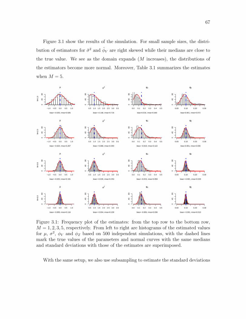
67
Figure 3.1 show the results of the simulation. For small sample sizes, the distri-
bution of estimators for σ2 and φV are right skewed while their medians are close to
the true value. We see as the domain expands (M increases), the distributions of
the estimators become more normal. Moreover, Table 3.1 summarizes the estimates
when M = 5.
µ
bias=−0.026, rmse=0.505
M=
1.0
−1.0 −0.5 0.0 0.5 1.0
040
80
σ2
bias=−0.148, rmse=0.716
0.5 1.0 1.5 2.0 2.5 3.0 3.5
040
80φV
bias=0.016, rmse=0.440
0.0 0.1 0.2 0.3 0.4 0.5
040
80
φZ
bias=0.001, rmse=0.072
0.00 0.10 0.20 0.30
040
80
µ
bias=−0.024, rmse=0.267
M=
2.0
−1.0 −0.5 0.0 0.5 1.0
040
80
σ2
bias=−0.068, rmse=0.393
0.5 1.0 1.5 2.0 2.5 3.0 3.5
040
80
φV
bias=−0.019, rmse=0.122
0.0 0.1 0.2 0.3 0.4 0.5
040
80
φZ
bias=0.001, rmse=0.030
0.00 0.10 0.20 0.30
040
80
µ
bias=−0.020, rmse=0.181
M=
3.0
−1.0 −0.5 0.0 0.5 1.0
040
80
σ2
bias=−0.026, rmse=0.253
0.5 1.0 1.5 2.0 2.5 3.0 3.5
040
80
φV
bias=−0.015, rmse=0.059
0.0 0.1 0.2 0.3 0.4 0.5
040
80
φZ
bias=−0.001, rmse=0.020
0.00 0.10 0.20 0.300
4080
µ
bias=−0.009, rmse=0.116
M=
5.0
−1.0 −0.5 0.0 0.5 1.0
040
80
σ2
bias=−0.004, rmse=0.159
0.5 1.0 1.5 2.0 2.5 3.0 3.5
040
80
φV
bias=−0.006, rmse=0.036
0.0 0.1 0.2 0.3 0.4 0.5
040
80
φZ
bias=−0.001, rmse=0.013
0.00 0.10 0.20 0.30
040
80
Figure 3.1: Frequency plot of the estimates: from the top row to the bottom row,M = 1, 2, 3, 5, respectively. From left to right are histograms of the estimated valuesfor µ, σ2, φV and φZ based on 500 independent simulations, with the dashed linesmark the true values of the parameters and normal curves with the same mediansand standard deviations with those of the estimates are superimposed.
With the same setup, we also use subsampling to estimate the standard deviations
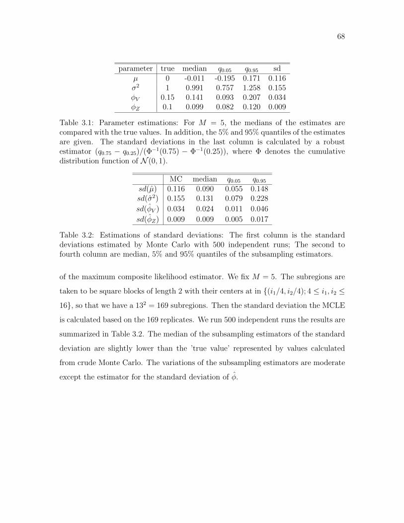
68
parameter true median q0.05 q0.95 sdµ 0 -0.011 -0.195 0.171 0.116σ2 1 0.991 0.757 1.258 0.155φV 0.15 0.141 0.093 0.207 0.034φZ 0.1 0.099 0.082 0.120 0.009
Table 3.1: Parameter estimations: For M = 5, the medians of the estimates arecompared with the true values. In addition, the 5% and 95% quantiles of the estimatesare given. The standard deviations in the last column is calculated by a robustestimator (q0.75 − q0.25)/(Φ−1(0.75) − Φ−1(0.25)), where Φ denotes the cumulativedistribution function of N (0, 1).
MC median q0.05 q0.95
sd(µ) 0.116 0.090 0.055 0.148sd(σ2) 0.155 0.131 0.079 0.228
sd(φV ) 0.034 0.024 0.011 0.046
sd(φZ) 0.009 0.009 0.005 0.017
Table 3.2: Estimations of standard deviations: The first column is the standarddeviations estimated by Monte Carlo with 500 independent runs; The second tofourth column are median, 5% and 95% quantiles of the subsampling estimators.
of the maximum composite likelihood estimator. We fix M = 5. The subregions are
taken to be square blocks of length 2 with their centers at in (i1/4, i2/4); 4 ≤ i1, i2 ≤
16, so that we have a 132 = 169 subregions. Then the standard deviation the MCLE
is calculated based on the 169 replicates. We run 500 independent runs the results are
summarized in Table 3.2. The median of the subsampling estimators of the standard
deviation are slightly lower than the ’true value’ represented by values calculated
from crude Monte Carlo. The variations of the subsampling estimators are moderate
except the estimator for the standard deviation of φ.
69
3.5 Proofs
3.5.1 Properties of the pairwise likelihood function of SHP
model
We present some uniform bounds for the pairwise log-likelihood function and its
partial derivatives that are are crucial to establish the asymptotic results for the
maximum composite likelihood estimator. Let ∂i denote the partial derivative with
respect to the i-th component of the parameter θ.
Proposition 24 Under Assumptions 16 and 17, there exist constants C ≥ 0, such
that for all s1 6= s2 ∈ Rm,
supθ∈Θ
∣∣ logfs2−s1(y1, y2; θ)∣∣ ≤ C
1− ρ∗(‖s2 − s1‖)(1 + y2
1 + y22), y1, y2 ∈ R.
Proposition 25 Under Assumptions 16 and 17, for any p ∈ N, and 1 ≤ i1, . . . , ip ≤
dim(θ), there exist constants C ≥ 0, such that for all s1 6= s2 ∈ Rm,
supθ∈Θ
∣∣∂i1 · · · ∂ip [logfs2−s1(y1, y2; θ)]∣∣ ≤ C
1− ρ∗(‖s2 − s1‖)p1+| log(y2
1)|2p+| log(y22)|2p, y1, y2 ∈ R.
Remark 4 Observe that for any p ∈ N,
E | log(Y 2(0))|p ≤ 2p−1E |V (0)|p + E | log(Z2(0))|p <∞,
and for any q ∈ N, a, b, c ≥ 0, (a + b + c)q ≤ 3q−1(aq + bq + cq). The uniform bound
in Proposition 25 implies that for any q ∈ N
E
(supθ∈Θ
∣∣∂i1 · · · ∂in [logfs2−s1(Y (s1), Y (s2); θ)]∣∣)q = O
(1− ρ∗(‖s2 − s1‖)−q
),
which is essential for obtaining uniform convergence results for composite log-likelihood
function and its derivatives and such uniform convergence is often required to guar-
antee consistency and asymptotic normality of MCLE.
70
The asymptotic results for the maximum composite likelihood estimator also rely
on the dependence structure of the pairwise log-likelihood function. We now introduce
the notions of κ-coefficients and the κ-weakly dependence adapted from Dedecker
et al. (2007). For any measurable function g : R × R × Rm × Rm → R, denote by
gs1,s2(y1, y2) = g(y1, y2; s1, s2), y1, y2 ∈ R and s1, s2 ∈ Rm. Then gs1,s2(Y (s1), Y (s2)) :
s1, s2 ∈ Rm is a random field living on the product space Rm×Rm. The distance in
between any two points (s1, s2) and (t1, t2) in Rm × Rm is defined as
d∗ ((s1, s2), (t1, t2)) = min‖si − tj‖ : i = 1, 2, j = 1, 2.3
Consider two subsets U, V ⊂ Rm × Rm. There cardinalities are |U | = I and
|V | = J . Let d∗(U, V ) = mind∗(s, t) : s ∈ U, t ∈ V . For some finite subset of
U ⊂ Rm × Rm, let
gU(Y ) = (gs1,s2(Y (s1), Y (s2)) : (s1, s2) ∈ U) ,
denote the finite dimensional random vector on U and
κY,g(U, V ) = sup0<Lip(h1),Lip(h2)<∞
|Cov (h1(gU(Y )), h2(gV (Y ))) ||U ||V |Lip(h1)Lip(h2)
,
where h1 : RI → R, h2 : RJ → R are Lipschitz functions with
Lip(h1)4= sup
x,y∈RI
|h1(x)− h1(y)|∑Ii=1 |xi − yi|
.
The κ-coefficient for the process gs1,s2(Y (s1), Y (s2)) : s1, s2 ∈ S is defined as
κY,g(l1, l2, r) = supκY,g(U, V ) : U, V ⊂ Rm × Rm, |U | ≤ l1, |V | ≤ l2, d∗(U, V ) ≥ r
(3.10)
where l1 and l2 are positive integers and r ≥ 0 and we write κY,g(r) = supl1,l2<∞ κY,g(l1, l2, r).
3Here d∗ is not a metric.

71
Proposition 26 Under Assumptions 16-19, for any θ ∈ Θ and
gs1,s2(y1, y2) = ω(s2 − s1) logfs2−s1(y1, y2; θ),
or
gs1,s2(y1, y2) = ω(s2 − s1)∂i1 · · · ∂ip [logfs2−s1(y1, y2; θ)] ,
where p ∈ N, and 1 ≤ i1, . . . , ip ≤ dim(θ), it follows that κY,g(r) = o(r−2m), as
r →∞.
3.5.2 Proofs for the main theorem
Lemma 27 Under Assumptions 15–21, we have
supθ∈Θ|CLn(θ)− E[CLn(θ)]| → 0 in L2 as n→∞.
Proof of Lemma 27. First for any fixed θ ∈ Θ, let
gs1,s2(y1, y2) = ω(s2 − s1) logfs2−s1(y1, y2; θ).
Then as a result of Proposition 24 and Assumption 19, we have, for any q > 2
sups1,s2∈Rm
E |gs1,s2(y1, y2)|q <∞.
By Proposition 26, κY,g(r) = o(m−2m). Further under Assumption 20, N is 2rN -
dependent. Therefore by the central limit theorem of Davis et al. (2014),
CLn(θ)− ECLn(θ) is AN(0,1
µ(Sn)ΣCL),
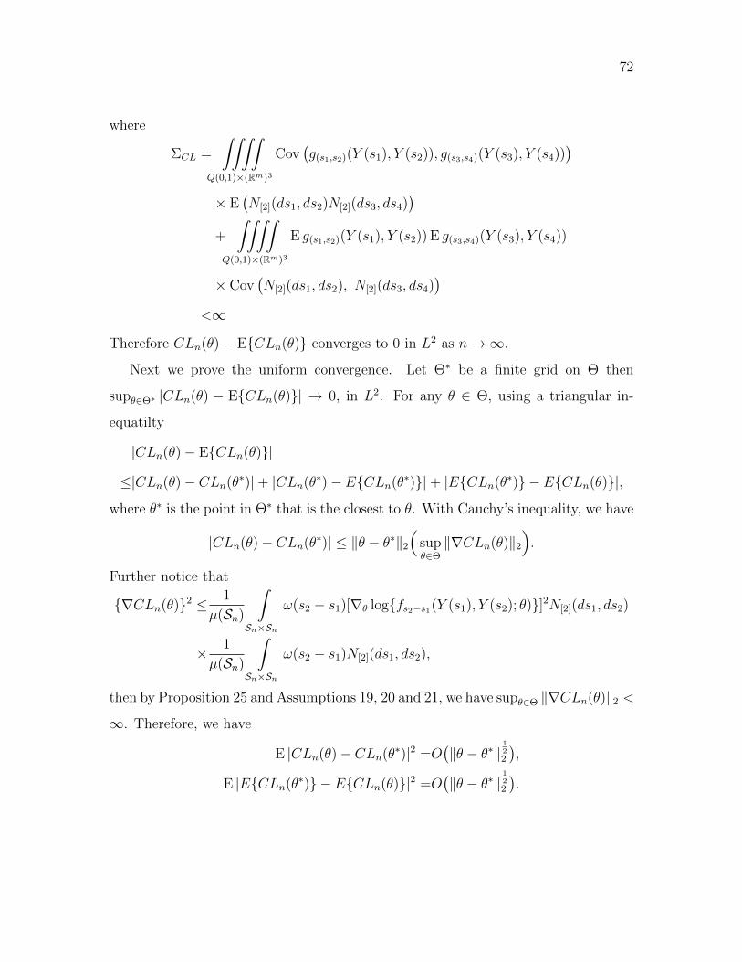
72
where
ΣCL =
∫∫∫∫Q(0,1)×(Rm)3
Cov(g(s1,s2)(Y (s1), Y (s2)), g(s3,s4)(Y (s3), Y (s4))
)× E
(N[2](ds1, ds2)N[2](ds3, ds4)
)+
∫∫∫∫Q(0,1)×(Rm)3
E g(s1,s2)(Y (s1), Y (s2)) E g(s3,s4)(Y (s3), Y (s4))
× Cov(N[2](ds1, ds2), N[2](ds3, ds4)
)<∞
Therefore CLn(θ)− ECLn(θ) converges to 0 in L2 as n→∞.
Next we prove the uniform convergence. Let Θ∗ be a finite grid on Θ then
supθ∈Θ∗ |CLn(θ) − ECLn(θ)| → 0, in L2. For any θ ∈ Θ, using a triangular in-
equatilty
|CLn(θ)− ECLn(θ)|
≤|CLn(θ)− CLn(θ∗)|+ |CLn(θ∗)− ECLn(θ∗)|+ |ECLn(θ∗) − ECLn(θ)|,
where θ∗ is the point in Θ∗ that is the closest to θ. With Cauchy’s inequality, we have
|CLn(θ)− CLn(θ∗)| ≤ ‖θ − θ∗‖2
(supθ∈Θ‖∇CLn(θ)‖2
).
Further notice that
∇CLn(θ)2 ≤ 1
µ(Sn)
∫Sn×Sn
ω(s2 − s1)[∇θ logfs2−s1(Y (s1), Y (s2); θ)]2N[2](ds1, ds2)
× 1
µ(Sn)
∫Sn×Sn
ω(s2 − s1)N[2](ds1, ds2),
then by Proposition 25 and Assumptions 19, 20 and 21, we have supθ∈Θ ‖∇CLn(θ)‖2 <
∞. Therefore, we have
E |CLn(θ)− CLn(θ∗)|2 =O(‖θ − θ∗‖
122
),
E |ECLn(θ∗) − ECLn(θ)|2 =O(‖θ − θ∗‖
122
).
73
So it follows supθ∈Θ |CLn(θ)− ECLn(θ)| → 0 in L2 as n→∞.
Proof of Proposition 20. (i) In the first part,
ECLn(θ) =1
µ(Sn)
∫Sn×Sn
ω(s2 − s1) E[logfs2−s1(Y (s1), Y (s2); θ)] EN[2](ds1, ds2)
=1
µ(Sn)
∫Sn×(Sn−Sn)
ω(u) E[logfu(Y (s1), Y (s1 + u); θ)] EN[2](ds1, d(s1 + u)),
where Sn − Sn = s2 − s1; s1, s2 ∈ Sn. Since∣∣ ∫Sn−Sn
ω(u) E[logfu(Y (s1), Y (s1 + u); θ)] EN[2](ds1, d(s1 + u))∣∣
≤∫Rm
ω(u) E | logfu(Y (s1), Y (s1 + u); θ)|EN[2](ds1, d(s1 + u))/ds1
and by Proposition 24 and Assumption 19,
sups1,u∈R
ω(u) E | logfu(Y (s1), Y (s1 + u); θ)| <∞.
Then by dominant convergence, limn→∞ ECLn(θ) = H(θ).
(ii)For fixed s1 and s2, by Jensen’s inequality
Eθ0
[log fs2−s1(Y (s1), Y (s2); θ)
fs2−s1(Y (s1), Y (s2); θ0)
]≤ log
[Eθ0
fs2−s1(Y (s1), Y (s2); θ)
fs2−s1(Y (s1), Y (s2); θ0)
]= 0
and therefore
E[
logfs2−s1(Y (s1), Y (s2); θ)
]≤ E
[logfs2−s1(Y (s1), Y (s2); θ0)
],
where equality holds if and only if almost surely fu(Y (0), Y (u); θ) = fu(Y (0), Y (u); θ0).
With the above inequality, immediately, it follows H(θ) ≤ H(θ0). The Assumption
22 guarantees that the equality holds only for θ = θ0.
Proof of Lemma 21 and Lemma 22. Just use similar argument as in the proof
of Lemma 27 and (i) in Proposition 20.
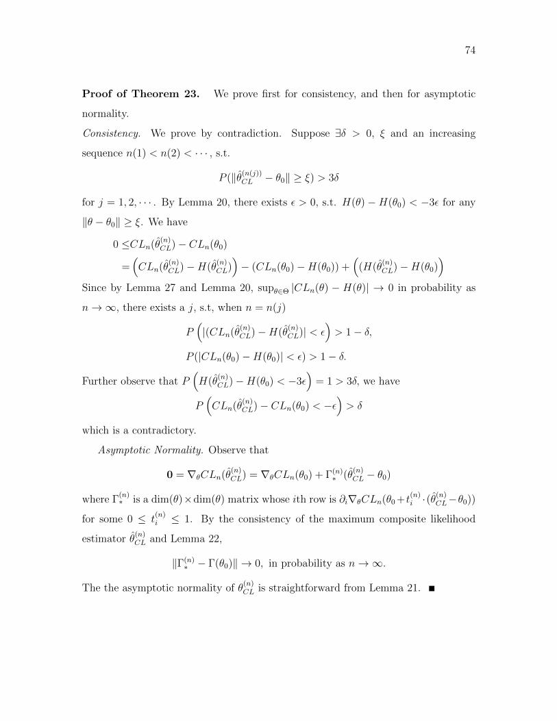
74
Proof of Theorem 23. We prove first for consistency, and then for asymptotic
normality.
Consistency. We prove by contradiction. Suppose ∃δ > 0, ξ and an increasing
sequence n(1) < n(2) < · · · , s.t.
P (‖θ(n(j))CL − θ0‖ ≥ ξ) > 3δ
for j = 1, 2, · · · . By Lemma 20, there exists ε > 0, s.t. H(θ)−H(θ0) < −3ε for any
‖θ − θ0‖ ≥ ξ. We have
0 ≤CLn(θ(n)CL)− CLn(θ0)
=(CLn(θ
(n)CL)−H(θ
(n)CL))− (CLn(θ0)−H(θ0)) +
((H(θ
(n)CL)−H(θ0)
)Since by Lemma 27 and Lemma 20, supθ∈Θ |CLn(θ) − H(θ)| → 0 in probability as
n→∞, there exists a j, s.t, when n = n(j)
P(|(CLn(θ
(n)CL)−H(θ
(n)CL)| < ε
)> 1− δ,
P (|CLn(θ0)−H(θ0)| < ε) > 1− δ.
Further observe that P(H(θ
(n)CL)−H(θ0) < −3ε
)= 1 > 3δ, we have
P(CLn(θ
(n)CL)− CLn(θ0) < −ε
)> δ
which is a contradictory.
Asymptotic Normality. Observe that
0 = ∇θCLn(θ(n)CL) = ∇θCLn(θ0) + Γ(n)
∗ (θ(n)CL − θ0)
where Γ(n)∗ is a dim(θ)×dim(θ) matrix whose ith row is ∂i∇θCLn(θ0 + t
(n)i ·(θ
(n)CL−θ0))
for some 0 ≤ t(n)i ≤ 1. By the consistency of the maximum composite likelihood
estimator θ(n)CL and Lemma 22,
‖Γ(n)∗ − Γ(θ0)‖ → 0, in probability as n→∞.
The the asymptotic normality of θ(n)CL is straightforward from Lemma 21.

75
3.5.3 Proof of Proposition 24
We will first establish bounds for the pairwise log-likelihood function at fix locations
s1 and s2. The bounds turns out to be continuous functions of the parameter θ and
‖s1 − s2‖. Hence with the compactness of the parameter space Θ and the support of
ω, we can extend these location-wise bounds to uniform bounds.
Lemma 28 With the pairwise likelihood function for two locations s1, s2 ∈ Rm de-
fined in (3.2),∣∣ logfs2−s1(y1, y2; θ)∣∣
≤ log(2π)− 1
2log(1− ρ2
Z
)+ |µ|+ 1 + ρV
4σ2 +
e−µ+σ2
2
2(1− |ρZ |)(y2
1 + y22
)Proof of Lemma 28. On one hand, for any y1, y2, θ,
logfs2−s1(y1, y2; θ)
≤ log∫∫
h0,0,s1,s2,θ(v1, v2)dv1dv2
= log
( 1
2π√
1− ρ2Z
EV
[exp−V (s1) + V (s2)
2])
=− log(2π)− 1
2log(1− ρ2
Z
)− µ+
1 + ρV4
σ2.

76
On the other hand, by Jensen’s inequality
logfs2−s1(y1, y2; θ)
≥∫∫
logfY (s1),Y (s2)|V (s1),V (s2)(y1, y2|v1, v2; θ, s1, s2)
fV (s1),V (s2)(v1, v2; θ, s1, s2)dv1dv2
≥− log(2π)− 1
2log(1− ρ2
Z
)− EV
y21e−V (s1) + y2
2e−V (s2) − 2ρZy1y2e
−V (s1)+V (s2)2
2(1− ρ2Z)
+V (s1) + V (s2)
2
=− log(2π)− 1
2log(1− ρ2
Z
)− µ− 1
2(1− ρ2Z)
(y2
1 + y22
)e−µ+σ2
2 − 2ρZy1y2e−µ+
1+ρV4
σ2≥− log(2π)− 1
2log(1− ρ2
Z
)− µ− 1
2(1− ρ2Z)
(1 + |ρZ |)(y2
1 + y22
)e−µ+σ2
2
Using the point-wise bound in Lemma 28, with Assumptions 16 and 17, the uni-
form bound in Proposition 24 follows.
3.5.4 Proof of Proposition 25
Following the same logic as the proof for Proposition 24, we will construct a point-
wise bound for the derivatives of the pairwise log-likelihood function and a uniform
bound will follow under Assumption 16 and 17. It is, however, more difficult to derive
bounds for the derivatives of the pairwise log-likelihood function. First using some
calculus, the problem can be reduced to deriving bounds for functions of the form
∂i1 · · · ∂infs2−s1/fs2−s1 . Then we relate these functions to conditional expectations
and bounds one them can be yield through the tail behavior of the conditional density
functions.
We will use the following notations in the statement of a coming lemma. For any
integers i1, i2, . . . , ip, let π denote a partition of these numbers
i(1, 1), . . . , i(1, l1), . . . , i(k, 1), . . . , i(1, lk)

77
in which i1, i2, . . . , ip are divided into k groups and each has l1, . . . , lk numbers and
we do not differentiate the order between and inside the groups. Denote by
∂πf =k∏j=1
∂i(j,1) · · · ∂i(j,lj)ff
Lemma 29 For any function f that is positive and n time differentiable with respect
to θ, we have
∂i1 · · · ∂iplog(f) =∑π
c(π)∂πf (3.11)
where the summation is taken over all partitions of i1, i2, . . . , ip and c(π) is some
constant only depends on π.
Proof of Lemma 29. With simple calculus one can verify that
∂ilog f =∂if
f,
∂i∂jlog f =∂i∂jf
f− ∂if
f· ∂jff,
∂i∂j∂klog f =∂i∂j∂kf
f− ∂i∂jf
f· ∂kff− ∂i∂kf
f· ∂jff− ∂j∂kf
f· ∂iff
+ 2∂if
f· ∂jff· ∂kff,
and the general form of (3.11) can be showed by induction.
To prove Proposition 25, it suffices to show that for any p ∈ N, 1 ≤ i1, . . . , ip ≤
dim(θ), and s1, s2 ∈ Rm with s1 6= s2, there exists a constant C(s1, s2) ≥ 0, such that
supθ∈Θ
∣∣∂i1 · · · ∂ipfs2−s1fs2−s1
(y1, y2; θ)∣∣ ≤ C(s1, s2)
(1− ρ∗)p1 + | log(y2
1)|2p + | log(y22)|2p, y1, y2 ∈ R.
(3.12)
and further
sup‖s1−s2‖≤rω
C(s1, s2) <∞,
where rω is a positive number for which ω(r) = 0 if r ≥ rω.
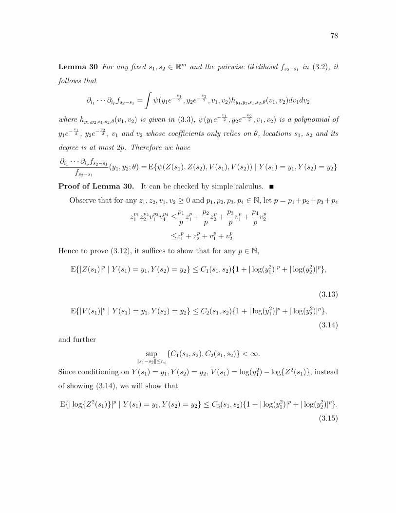
78
Lemma 30 For any fixed s1, s2 ∈ Rm and the pairwise likelihood fs2−s1 in (3.2), it
follows that
∂i1 · · · ∂ipfs2−s1 =
∫ψ(y1e
− v12 , y2e
− v22 , v1, v2)hy1,y2,s1,s2,θ(v1, v2)dv1dv2
where hy1,y2,s1,s2,θ(v1, v2) is given in (3.3), ψ(y1e− v1
2 , y2e− v2
2 , v1, v2) is a polynomial of
y1e− v1
2 , y2e− v2
2 , v1 and v2 whose coefficients only relies on θ, locations s1, s2 and its
degree is at most 2p. Therefore we have
∂i1 · · · ∂ipfs2−s1fs2−s1
(y1, y2; θ) = Eψ(Z(s1), Z(s2), V (s1), V (s2)) | Y (s1) = y1, Y (s2) = y2
Proof of Lemma 30. It can be checked by simple calculus.
Observe that for any z1, z2, v1, v2 ≥ 0 and p1, p2, p3, p4 ∈ N, let p = p1 +p2 +p3 +p4
zp11 zp22 v
p31 v
p44 ≤
p1
pzp1 +
p2
pzp2 +
p3
pvp1 +
p4
pvp2
≤zp1 + zp2 + vp1 + vp2
Hence to prove (3.12), it suffices to show that for any p ∈ N,
E|Z(s1)|p | Y (s1) = y1, Y (s2) = y2 ≤ C1(s1, s2)1 + | log(y21)|p + | log(y2
2)|p,
(3.13)
E|V (s1)|p | Y (s1) = y1, Y (s2) = y2 ≤ C2(s1, s2)1 + | log(y21)|p + | log(y2
2)|p,
(3.14)
and further
sup‖s1−s2‖≤rω
C1(s1, s2), C2(s1, s2) <∞.
Since conditioning on Y (s1) = y1, Y (s2) = y2, V (s1) = log(y21)− logZ2(s1), instead
of showing (3.14), we will show that
E| logZ2(s1)|p | Y (s1) = y1, Y (s2) = y2 ≤ C3(s1, s2)1 + | log(y21)|p + | log(y2
2)|p.
(3.15)
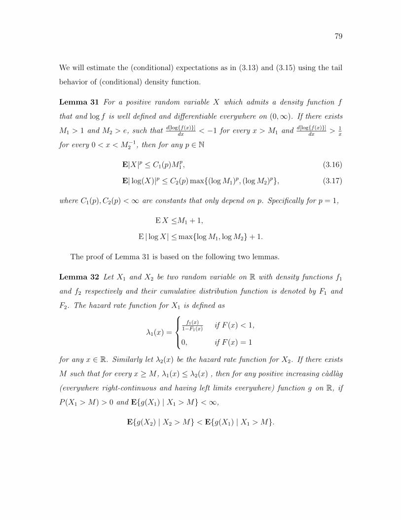
79
We will estimate the (conditional) expectations as in (3.13) and (3.15) using the tail
behavior of (conditional) density function.
Lemma 31 For a positive random variable X which admits a density function f
that and log f is well defined and differentiable everywhere on (0,∞). If there exists
M1 > 1 and M2 > e, such that d[logf(x)]dx
< −1 for every x > M1 and d[logf(x)]dx
> 1x
for every 0 < x < M−12 , then for any p ∈ N
E|X|p ≤ C1(p)Mp1 , (3.16)
E| log(X)|p ≤ C2(p) max(logM1)p, (logM2)p, (3.17)
where C1(p), C2(p) <∞ are constants that only depend on p. Specifically for p = 1,
EX ≤M1 + 1,
E | logX| ≤maxlogM1, logM2+ 1.
The proof of Lemma 31 is based on the following two lemmas.
Lemma 32 Let X1 and X2 be two random variable on R with density functions f1
and f2 respectively and their cumulative distribution function is denoted by F1 and
F2. The hazard rate function for X1 is defined as
λ1(x) =
f1(x)
1−F1(x)if F (x) < 1,
0, if F (x) = 1
for any x ∈ R. Similarly let λ2(x) be the hazard rate function for X2. If there exists
M such that for every x ≥M , λ1(x) ≤ λ2(x) , then for any positive increasing cadlag
(everywhere right-continuous and having left limits everywhere) function g on R, if
P (X1 > M) > 0 and Eg(X1) | X1 > M <∞,
Eg(X2) | X2 > M < Eg(X1) | X1 > M.
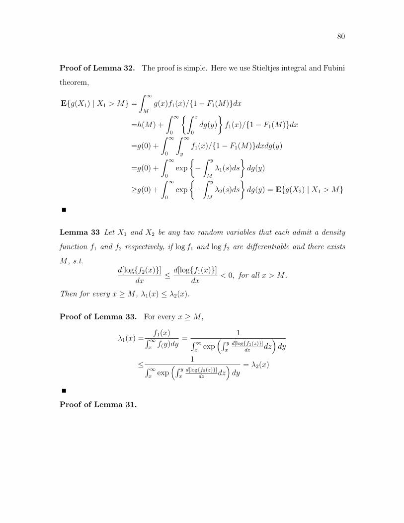
80
Proof of Lemma 32. The proof is simple. Here we use Stieltjes integral and Fubini
theorem,
Eg(X1) | X1 > M =
∫ ∞M
g(x)f1(x)/1− F1(M)dx
=h(M) +
∫ ∞0
∫ x
0
dg(y)
f1(x)/1− F1(M)dx
=g(0) +
∫ ∞0
∫ ∞y
f1(x)/1− F1(M)dxdg(y)
=g(0) +
∫ ∞0
exp
−∫ y
M
λ1(s)ds
dg(y)
≥g(0) +
∫ ∞0
exp
−∫ y
M
λ2(s)ds
dg(y) = Eg(X2) | X1 > M
Lemma 33 Let X1 and X2 be any two random variables that each admit a density
function f1 and f2 respectively, if log f1 and log f2 are differentiable and there exists
M , s.t.d[logf2(x)]
dx≤ d[logf1(x)]
dx< 0, for all x > M .
Then for every x ≥M , λ1(x) ≤ λ2(x).
Proof of Lemma 33. For every x ≥M ,
λ1(x) =f1(x)∫∞
xf(y)dy
=1∫∞
xexp
(∫ yxd[logf1(z)]
dzdz)dy
≤ 1∫∞x
exp(∫ y
xd[logf2(z)]
dzdz)dy
= λ2(x)
Proof of Lemma 31.
81
1. If there exist M1 > 1, s.t. d[logf(x)]dx
< −1 for every x > M1, then by Lemma
32 and 33, X will have a right tail lighter than Exp(1),
E(|X −M1|p | X > M1) ≤ Γ(p+ 1), for any p > 0,
E(| logX − logM1|p | X > M1) ≤ 1
M1
Γ(p+ 1), for any p > 0,
where Γ(p+ 1) =∫∞
0e−xxpdx is the Gamma function.
2. If there exist M2 > e, s.t. d[logf(x)]dx
x > 1x
for every x < M2, then X will have
a left tail lighter than X∗ whose density fX∗(x) = 2x10≤x≤1,
E(| − logX − logM2|p | 0 < X < M−12 ) ≤ 1
2p+1Γ(p+ 1), for any p > 0
Finally, with the binomial expansion with 0 ≤ b ≤ a,
ap =
p∑i=0
(p
i
)bi(a− b)p−i,
we conclude that (3.16) and (3.17) hold.
Now we are ready to prove (3.13) and (3.15). Conditioning on Y (s1) = y1, Y (s2) =
y2, y1y2 6= 0, the density function of conditional distribution of (Z1 = Z(s1), Z2 =
Z(s2)) is
h1,2(z1, z2) ∝ 1
2π√
1− ρ2Z
e− z
21+z
22−2ρzz1z2
2(1−ρ2z) × 4
|y1y2|
× 1
2π√
1− ρ2V
e− (log y21−log z21−µ)
2+(log y22−log z22−µ)2−2ρV (log y21−log z21−µ)(log y
22−log z22−µ)
2(1−ρ2V
)σ2 .
where z1, z2 has the same sign with y1, y2 respectively. Without loss of generality,
we assume y1, y2 > 0 (as in the other three case, the analysis is similar). Let h1(z1)
and h2(z2) be the marginal density function of Z1 and Z2, conditioning on Y (s1) =

82
y1, Y (s2) = y2. As indicated in lemma 31, the key step is to evaluate
∂[logh1(z1)]∂z1
=
∂∫h1,2(z1,z2)dz2
∂z1
h1(z1)=
∫ ∂[logh1,2(z1,z2)]∂z1
h1,2(z1, z2)dz2
h1(z1)
=Eh
(∂[logh1,2(Z1, Z2)]∂z1
| Z1 = z1
),
where the expectation is with respect to the joint density function h1,2. Since
∂[logh1,2(Z1, Z2)]∂z1
=− z1
1− ρ2Z
+ρZz2
1− ρ2Z
+log(y2
1)− ρV log(y22)− log(z2
1) + ρa log(z22)− (1− ρV )µ
(1− ρ2V )σ2
· 2
z1
,
it follows that
∂[logh1(z1)]∂z1
=− z1
1− ρ2Z
+ρZEh(Z2 | Z1 = z1)
1− ρ2Z
+log(y2
1)− ρV log(y22)− log(z2
1) + ρV Ehlog(Z22) | Z1 = z1 − (1− ρV )µ
(1− ρ2V )σ2
· 2
z1
(3.18)
To evaluate Eh(Z2 | Z1 = z1) and Ehlog(Z22) | Z1 = z1 in the above expression, we
need to analyse the conditional density of Z2 given Z1 = z1,
h2|1(z2|z1) ∝e− (z2−ρZz1)
2
2(1−ρ2Z)− [log(y22)−log(z22)−µ−ρV log(y
21)−log(z21)−µ]
2
2(1−ρ2V
)σ2
and the derivative of its logarithm is
∂[logh2|1(z2|z1)]∂z2
= −z2 − ρZz1
1− ρ2Z
+log(y2
2)− log(z22)− µ − ρV log(y2
1)− log(z21)− µ
(1− ρ2V )σ2
· 2z2
(3.19)
Now we try to evaluate (3.18) the analyse breaks into two cases.
i. On the right tail: If z1 >4| log(y21)|+| log(y22)|+2|µ|+3+log( 1
1+ρZ)
(1−ρ2V )σ2 +16+ 41−ρZ
, ∂[logh1(z1)]∂z1
<
−1. We use the following bounds
Eh(Z2 | Z1 = z1) ≤3 + ρZ4
z1 + 1,
Eh(Z2 | Z1 = z1) ≥0,
(3.20)

83
and
Eh(log(Z22) | Z1 = z1) ≤ log(z2
1) + 1,
Eh(log(Z22) | Z1 = z1) ≥− log(z2
1)− | log(y21)| − | log(y2
2)| − 2|µ| − (1− ρ2V )σ2 + 2 log(1 + ρZ)− 3.
(3.21)
With (3.20), it follows that
− z1
1− ρ2Z
+ρZEh(Z2 | Z1 = z1)
1− ρ2Z
≤− z1
1− ρ2Z
+3+ρZ
4z1 + 1
1− ρ2Z
= −1−ρZ
4z1 − 1
1− ρ2Z
≤ −2.
With (3.21), it follows that
log(y21)− ρa log(y2
2)− log(z21) + ρV Ehlog(Z2
2) | Z1 = z1 − (1− ρV )µ
(1− ρ2V )σ2
· 2
z1
≤2| log(y2
1)|+ 2| log(y22)|+ 4|µ|+ (1− ρ2
V )σ2 + 2 log( 11+ρZ
) + 3
(1− ρ2V )σ2
· 2
z1
< 1.
Combine the above two inequality we have ∂[logh1(z1)]∂z1
< −1. To prove (3.20) and
(3.21), we use Lemma 31 and examine the two tails of Z2 give Z1 = z1.
When z2 >3+ρz
4z1, we have
−z2 − ρZz1
1− ρ2Z
≤ −3(1−ρZ)
4z1
1− ρ2Z
< −3,
and
log(y22)− log(z2
2)− µ − ρV log(y21)− log(z2
1)− µ(1− ρ2
V )σ2· 2
z2
≤ | log(y21)|+ | log(y2
2)| − log z21 + 2 + log z2
1 + 2|µ|)(1− ρ2
V )σ2· 2
z2
≤ | log(y21)|+ | log(y2
2)|+ 2 + 2|µ|)(1− ρ2
V )σ2· 4
z1
< 1.
Combine the above two inequality, with (3.19) it follows that∂ logh2|1(z2|z1)
∂z2< −1.
Therefore (3.20) holds and Ehlog(Z22) | Z1 = z1 ≤ log(z2
1) + 1.

84
When log(z22) < − log(z2
1)−| log(y21)|−| log(y2
2)|−2|µ|−(1−ρ2V )σ2+2 log(1+ρZ)−2,
we have
(log(y22)− log(z2
2)− µ)− ρV (log(y21)− log(z2
1)− µ)
(1− ρ2V )σ2
· 2
z2
>2
z2
,
and
−z2 − ρZz1
1− ρ2Z
>−z1 + ρZz1
1− ρ2Z
> − z1
1 + ρZ> − 1
z2
.
Combine the above two inequality we have∂ logh2|1(z2|z1)
∂z2> 1
z2and (3.21) follows.
ii. On the left tail: If
log z21 <−
| log(y21)|+ | log(y2
2)|+ 2|µ|+ 1
(1− |ρV |)− (1 + |ρV |)σ2 − 2 log
2
1− ρ2Z
− 2 log[ 3√
1− ρ2Z
+2 1
σ2 + 1(1−ρ2V )σ2
1− ρ2Z
],
then ∂[logh1(z1)]∂z1
> 1z1. We use the following bounds
Eh(Z2 | Z1 = z1) ≤2 + 3(1− ρ2Z) +
| log(y21)|+ | log(y2
2)|+ 2|µ|+ | log(z21)|
(1− ρ2V )σ2
Eh(Z2 | Z1 = z1) ≥0
(3.22)
and
Ehlog(Z22) | Z1 = z1 ≤| log(z2
1)|+ 1
Ehlog(Z22) | Z1 = z1 ≥ − | log(z2
1)| − 1(3.23)
With (3.22), we have
− z1
1− ρ2Z
+ρZEh(Z2|Z1 = z1)
1− ρ2Z
>−1− 2− 3(1− ρ2
Z)− | log(y21)|+| log(y22)|+2|µ|+| log(z21)|(1−ρ2V )σ2
1− ρ2Z
>− 6
1− ρ2Z
−1σ2 + 1
(1−ρ2a)σ2
1− ρ2Z
| log z21 | > −
1
z,

85
where in the last inequality we used fact that for any a, b > 0 and x > (√a+ b)2, an
inequality holds that
x > a+ b log(x).
With (3.23), we have
log(y21)− ρV log(y2
2)− log(z21) + ρV Ehlog(Z2
2) | Z1 = z1 − (1− ρV )µ
(1− ρ2V )σ2
>−| log(y2
1)| − | log(y22)| − log(z2
1) + |ρa| log(z21)− 1− 2|µ|
(1− ρ2a)σ
2> 1
Combine the above two inequality, with (3.18), it follows that ∂[logh1(z1)]∂z1
> 1z1. To
prove (3.22) and (3.23), we use Lemma 31 and examine the two tails of Z2 give
Z1 = z1.
When z2 > 1 + 3(1− ρ2Z) +
| log(y21)|+| log(y22)|+2|µ|+| log(Z21 )|
(1−ρ2V )σ2 , we have
−z2 − ρZz1
1− ρ2Z
< −3
and
log(y22)− log(z2
2)− µ − ρV log(y21)− log(z2
1)− µ(1− ρ2
V )σ2· 2
z2
<| log(y2
1)|+ | log(y22)|+ | log z2
1 |+ 2|µ|(1− ρ2
a)σ2
· 2
z2
< 2
so that∂ log h2|1(z2|z1)
∂z2< −1, which in turn (3.22) holds, and further
Eh(log(Z22) | Z1 = z1) ≤2 log1 + 3(1− ρ2
Z) +| log(y2
1)|+ | log(y22)|+ 2|µ|+ | log(z2
1)|(1− ρ2
V )σ2+ 1
<2 log[4 + 1
σ2+
1
(1− ρ2V )σ2
| log z21 |]
+ 1
<2 log1
z1
+ 1 = − log(z21) + 1.
When z2 < z1, we have
−z2 − ρZz1
1− ρ2Z
> − 2
1− ρ2Z
> − 1
z1
> − 1
z2

86
and
(log(y22)− log(z2
2)− µ)− ρV (log(y21)− log(z2
1)− µ)
(1− ρ2V )σ2
>−(1− |ρV |) log z2
1 − | log(y21)| − | log(y2
2)| − 2|µ|)(1− ρ2
V )σ2> 1
Combine the above two inequality, with (3.19) it follows that∂ logh2|1(z2|z1)
∂z2> 1
z2, so
that
Eh(log(Z22) | Z1 = z1) ≥ log(z2
1)− 1,
and (3.23) holds.
Combining the results on the right tail and the left tail, with Lemma 31, we
conclude (3.13) and (3.15) hold.
3.5.5 κ-weak dependence of the SHP model
Proposition 34 For any Gaussian random field Y (s); s ∈ Rm on Rm,
κY (l1, l2, r) = sups,t∈Rm,‖s−t‖≥r
|Cov(Y (s), Y (t))|, l1, l2 ∈ Z+, r ≥ 0.
Proof of Proposition 34. Refer to Davis et al. (2014).
Proposition 35 Let Y be the SHP model on Rm defined in (3.1), then for any 0 <
δ < 1,
κY (r) = O(ρV (r)1−δ) +O(ρZ(r)1−δ), l1, l2 ∈ Z+, r ≥ 0.
The proof of Proposition 35 relies on the following results.
Lemma 36 Let Xi, X′i, Zj, Z
′j, 1 ≤ i ≤ I, 1 ≤ j ≤ J , I, J ∈ Z+ be random
variables that are bounded in L2 norm, and h1, h2 are Lipschitz functions on RI and
87
RJ respectively. The following inequality always holds
|Covh1(Xi, 1 ≤ i ≤ I)− h1(X ′i, 1 ≤ i ≤ I), h2(Zj, 1 ≤ j ≤ J)− h2(Z ′j, 1 ≤ j ≤ J)
|
≤IJLip(h1)Lip(h2) sup1≤i≤I
‖Xi −X ′i‖2 sup1≤j≤J
‖Zj − Z ′j‖2
where ‖ · ‖2 denote the L2 norm of a random variable, i.e. ‖X‖24= (EX2)
12 for any
random variable X. Further, by taking Z ′j = EZj, 1 ≤ j ≤ J , it immediately holds
that
|Cov (h1(Xi, 1 ≤ i ≤ I)− h1(X ′i, 1 ≤ i ≤ I), h2(Zj, 1 ≤ j ≤ J)) |
≤IJLip(h1)Lip(h2) sup1≤i≤I
‖Xi −X ′i‖2 sup1≤j≤J
(VarZj)12
Proof of Lemma 36. Refer to Davis et al. (2014).
Lemma 37 For function f , suppose there exists some function f∗ : [0,∞)→ R with
the following properties:
1. f∗(0) = 1;
2. f∗ is differentiable. Its derivative f ′∗ is a non-decreasing function on [0,∞);
3. For any 0 ≤ y1 ≤ y2,
|f(y2)− f(y1)| ≤ f∗(y2)− f∗(y1),
and for any y2 ≤ y1 ≤ 0,
|f(y2)− f(y1)| ≤ f∗(|y2|)− f∗(|y1|).
If there exists constant K > 0 such that, f ′∗(y) < Kf∗(y) for any y ≥ 0, i. e.
(log f∗)′ < K on [0,∞) and M∗
p
4= sups∈Rm E (f∗(Y (s)))p < ∞ for some p > 2, then
88
with W (s) = f(Y (s)), s ∈ Rm, for any positive integers l1, l2 and distance r > 0,
κW (l1, l2, r) ≤
(p2
+ 1) (
p−22
)− p−2p+2(M∗
p
) 2p K
2(p−2)p+2 κY (l1, l2, r)
p−2p+2 ,
if κY (l1, l2, r) ≤(p2− 1) (M∗
p
) 12
+ 1p K−2,(
M∗p
) 2p , o.w.
Proof of Lemma 37. For any positive integers l1, l2 and distance r > 0,
κW (l1, l2, r) ≤ sups∈Rm
Var (f(Y ))
≤ sups∈Rm
E (f∗(Y ))2 ≤(M∗
p
) 2p .
Let U , V be any subsets of Rm such that ](U) = I ≤ l1, ](V ) = J ≤ l2, d(U, V ) ≥ r
and h1, h2 are Lipschitz functions on RI and RJ respectively.
For any M > 0, denote by
Y (M)(s) = (Y (s) ∧M) ∨ (−M) , s ∈ Rm.
Notice the following decomposition
Cov (h1 (f(Y (s)), s ∈ U) , h2 (f(Y (r)), t ∈ V ))
=Cov(h1
(f(Y (M)(s)), s ∈ U
), h2
(f(Y (M)(r)), t ∈ V
))+ Cov
(h1 (f(Y (s)), s ∈ U)− h1
(f(Y (M)(s)), s ∈ U
), h2 (f(Y (r)), t ∈ V )
)+ Cov
(h1
(f(Y (M)(s)), s ∈ U
), h2 (f(Y (r)), t ∈ V )− h2
(f(Y (M)(r)), t ∈ V
))4=Q1 +Q2 +Q3
For the first term, since f(Y (M)(s)) is a Lipschitz function of Y (M),
|Q1|IJLip(h1)Lip(h2)
≤ (f ′∗(M))2κY (I, J, r) ≤ K2 (f∗(M))2 κY (I, J, r).

89
For the second term,
|Q2|IJLip(h1)Lip(h2)
≤[sups∈U
Ef(Y (s))− f(Y (M)(s))2
] 12
×[supt∈V
Ef(Y (t))− f(0)2
] 12
Since for any s
E(f(Y (s))− f(Y (M)(s))
)2 ≤ E(f∗(Y (s))− f∗(Y (M)(s))
)2 ≤M∗
p
(f∗(M))p−2
E (f(Y (s))− f(0))2 ≤(M∗
p
) 2p
it immediate follows,
|Q2| ≤ IJLip(h1)Lip(h2)(M∗
p
) 12
+ 1p (f∗(M))1− p
2 .
Similarly for the third term, we have the same bound,
|Q3| ≤ IJLip(h1)Lip(h2)(M∗
p
) 12
+ 1p (f∗(M))1− p
2 .
The above derivation holds for any U, V and h1, h2 so that
κW (l1, l2, r) ≤ 2(M∗
p
) 12
+ 1p (f∗(M))1− p
2 +K2 (f∗(M))2 κY (l1, l2, r),
by taking f∗(M) =((
p2− 1) (M∗
p
) 12
+ 1p K−2κ−1
Y (l1, l2, r)) 2p+2
, we have
κW (l1, l2, r) ≤(p
2+ 1)(p− 2
2
)− p−2p+2 (
M∗p
) 2p K
2(p−2)p+2 κY (l1, l2, r)
p−2p+2
Lemma 38 Suppose Y1(s); s ∈ Rm and Y2(s); s ∈ Rm are two independent ran-
dom fields on Rm and W (s) = Y1(s)Y2(s); s ∈ Rm. If Mp = supE |Y1(s)|p,E |Y2(s)|p; s ∈
Rm <∞, then the κ-coefficient of W satisfies:
κW (l1, l2, r) ≤ (p− 2)−p−2p+2 (p+ 2)M
2(p+6)p(p+2)p (κY1(l1, l2, r) + κY2(l1, l2, r))
p−2p+2 , l1, l2 ∈ Z+, r ≥ 0
90
Proof of Lemma 38. For any M > 0, let
Y(M)
1 (s) = (Y1(s) ∧M) ∨ (−M), Y(M)
1 (s) = Y1(s)− Y (M)1 (s),
W (M)(s) = Y(M)
1 (s)Y(M)
2 (s), W(M)1 (s) = W (s)−W (M)(s)
Still use similar decomposition as before
Cov (h1(WU), h2(WV )) =Cov(h1(W
(M)U ), h2(W
(M)V )
)+ Cov
(h1(WU)− h1(W
(M)U ), h2(WV )
)+ Cov
(h1(W
(M)U ), h2(WV )− h2(W
(M)V )
)4=Q1 +Q2 +Q3
Since product is a Lipshitz function in any bounded region of R2,
|Q1| ≤ IJLip(h1)Lip(h2)M2 (κY1(l1, l2, r) + κY2(l1, l2, r)) .
For the second term,
|Q2|IJLip(h1)Lip(h2)
≤(
sups∈Rm
E(W (s)−W (M)(s)
)2) 1
2(
sups∈Rm
EW 2(s)
) 12
.
While for any s ∈ Rm
EW 2(s) = EY 21 (s) EY 2
2 (s) ≤M4pp
and
E(W (s)−W (M)(s)
)2
≤2 E(Y1(s)− Y (M)
1 (s))2
Y 22 (s) + 2 E
(Y
(M)1 (s)
)2 (Y2(s)− Y (M)
2 (s))2
=2 E(Y1(s)− Y (M)
1 (s))2
EY 22 (s) + 2 E
(Y
(M)1 (s)
)2
E(Y2(s)− Y (M)
2 (s))2
≤4M1+ 2
pp M2−p,

91
It follows
|Q2| ≤ IJLip(h1)Lip(h2) · 2M12
+ 3p
p M1− p2
The same bound also holds for Q3. So that
κW (l1, l2, r) ≤M2 (κY1(l1, l2, r) + κY2(l1, l2, r)) + 4M12
+ 3p
p M1− p2 ,
by taking M =
((p− 2)M
12
+ 3p
p (κY1(l1, l2, r) + κY2(l1, l2, r))−1
) 2p+2
κW (l1, l2, r) ≤ (p− 2)−p−2p+2 (p+ 2)M
2(p+6)p(p+2)p (κY1(l1, l2, r) + κY2(l1, l2, r))
p−2p+2
Proof of Proposition 35. By lemma 37, let Y1 = eV/2, then κY1(r) = O(ρV (r)1− δ2 ).
Let Y2 = Z, then κY2(r) = O(ρ(r)). Then apply Lemma 38 we conclude the result.
3.5.6 Proof of Proposition 26
Lemma 39 For any fixed s1, s2 ∈ Rm and the pairwise likelihood fs2−s1 in (3.2),
p ∈ N ∪ 0, 1 ≤ i1, . . . , ip ≤ dim(θ), we have
∂y1∂i1 · · · ∂ipfs2−s1fs2−s1
(y1, y2; θ) =1
y1
Eφ(Z(s1), Z(s2), V (s1), V (s2)) | Y (s1) = y1, Y (s2) = y2,
∂y2∂i1 · · · ∂ipfs2−s1fs2−s1
(y1, y2; θ) =1
y2
Eφ(Z(s2), Z(s1), V (s2), V (s1)) | Y (s1) = y1, Y (s2) = y2,
where ∂y1 and ∂y2 denote the partial derivative with respect to y1, y2 respectively, and
φ is polynomial whose coefficients only relies on θ, locations s1, s2 and its degree is
at most 2p+ 1.
Proof of Lemma 39. Similar to Lemma 30 it can be checked by simple calculus.
92
Lemma 40 Under Assumptions 16 and 17, for any p ∈ N∪0, and 1 ≤ i1, . . . , ip ≤
dim(θ), there exist constants C ≥ 0, such that for any s1 6= s2 ∈ Rm,
supθ∈Θ
∣∣∂y1∂i1 · · · ∂ip [logfs2−s1(y1, y2; θ)]∣∣ ≤ C
y11− ρ∗(‖s2 − s1‖)p1 + | log(y2
1)|2p+1 + | log(y22)|2p+1,
supθ∈Θ
∣∣∂y2∂i1 · · · ∂ip [logfs2−s1(y1, y2; θ)]∣∣ ≤ C
y21− ρ∗(‖s2 − s1‖)p1 + | log(y2
1)|2p+1 + | log(y22)|2p+1,
y1, y2 ∈ R.
Proof of Lemma 40. With Lemma 39, the proof for Lemma 40 is essentially the
same with Proposition 25 therefore omitted.
Now we proof Proposition 26. We first prove for
gs1,s2(y1, y2) = ω(s2 − s1)∂i1 · · · ∂ip [logfs2−s1(y1, y2; θ)] .
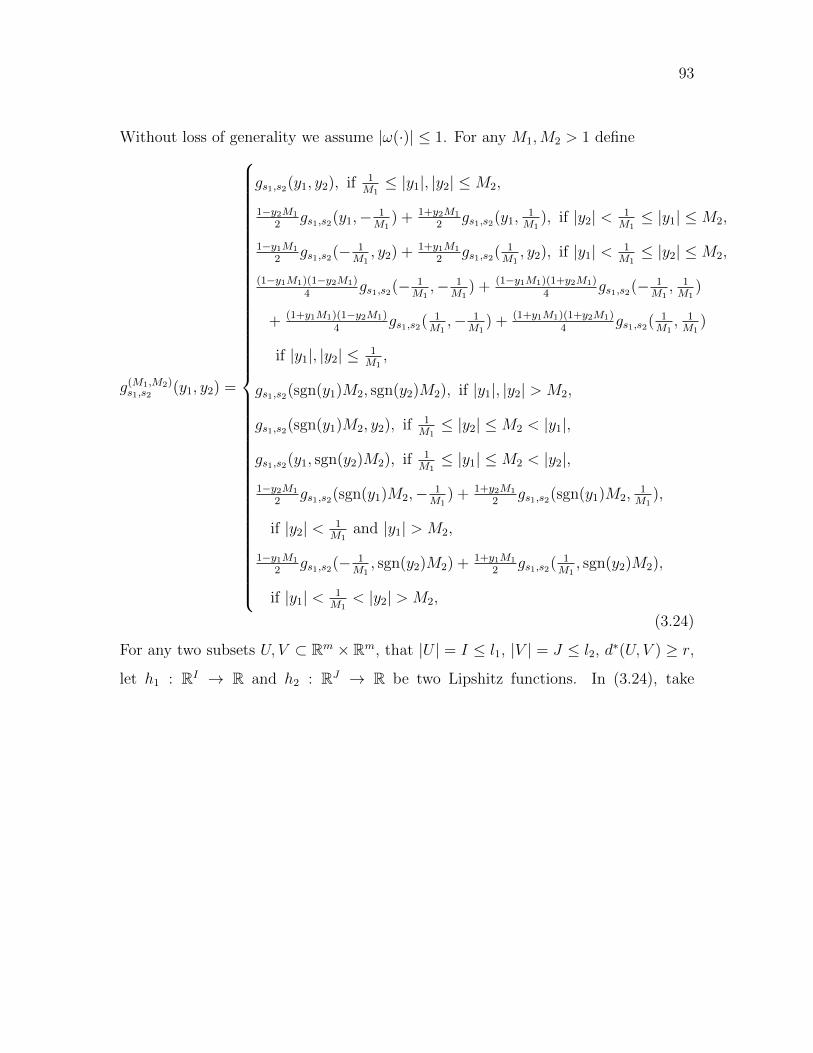
93
Without loss of generality we assume |ω(·)| ≤ 1. For any M1,M2 > 1 define
g(M1,M2)s1,s2
(y1, y2) =
gs1,s2(y1, y2), if 1M1≤ |y1|, |y2| ≤M2,
1−y2M1
2gs1,s2(y1,− 1
M1) + 1+y2M1
2gs1,s2(y1,
1M1
), if |y2| < 1M1≤ |y1| ≤M2,
1−y1M1
2gs1,s2(− 1
M1, y2) + 1+y1M1
2gs1,s2(
1M1, y2), if |y1| < 1
M1≤ |y2| ≤M2,
(1−y1M1)(1−y2M1)4
gs1,s2(− 1M1,− 1
M1) + (1−y1M1)(1+y2M1)
4gs1,s2(− 1
M1, 1M1
)
+ (1+y1M1)(1−y2M1)4
gs1,s2(1M1,− 1
M1) + (1+y1M1)(1+y2M1)
4gs1,s2(
1M1, 1M1
)
if |y1|, |y2| ≤ 1M1
,
gs1,s2(sgn(y1)M2, sgn(y2)M2), if |y1|, |y2| > M2,
gs1,s2(sgn(y1)M2, y2), if 1M1≤ |y2| ≤M2 < |y1|,
gs1,s2(y1, sgn(y2)M2), if 1M1≤ |y1| ≤M2 < |y2|,
1−y2M1
2gs1,s2(sgn(y1)M2,− 1
M1) + 1+y2M1
2gs1,s2(sgn(y1)M2,
1M1
),
if |y2| < 1M1
and |y1| > M2,
1−y1M1
2gs1,s2(− 1
M1, sgn(y2)M2) + 1+y1M1
2gs1,s2(
1M1, sgn(y2)M2),
if |y1| < 1M1
< |y2| > M2,
(3.24)
For any two subsets U, V ⊂ Rm × Rm, that |U | = I ≤ l1, |V | = J ≤ l2, d∗(U, V ) ≥ r,
let h1 : RI → R and h2 : RJ → R be two Lipshitz functions. In (3.24), take

94
M1 = M2 = M > 1, we have
Covh1(g(Y, U)), h2(g(Y, V ))
=Covh1(g(M,M)(Y, U)), h2(g(M,M)(Y, V ))
+ Covh1(g(Y, U))− h1(g(M,M)(Y, U)), h2(g(Y, V ))
+ Covh1(g(M,M)(Y, U)), h2(g(Y, V ))− h2(g(M,M)(Y, V ))4=Q1 +Q2 +Q3
Firstly we have
|Q1|IJLip(h1)Lip(h2)
≤ 4Lip(g(M,M))2κY (2l1, 2l2, r)
where
Lip(g(M,M)) = sups1,s2
Lip(g(M,M)s1,s2
).
As a consequence of Proposition 25 and Lemma 40, for any δ > 0, there exists a
constant C5 > 0 such that for any s1, s2,
Lip(g(M,M)s1,s2
) ≤ maxM [C3 + 2C4log(M2)2p+1],M [C1 + 2C2log(M2)2p] < C5M1+δ
Secondly
|Q2|IJLip(h1)Lip(h2)
≤[
sup(s1,s2)∈U
Egs2−s1(Y (s1), Y (s2))− g(M,M)s2−s1 (Y (s1), Y (s2))2
] 12
×[
sup(s1,s2)∈V
Egs2−s1(Y (s1), Y (s2))2] 1
2 .
On one hand, Proposition 25 and Assumption 19 induce that
sup(s1,s2)∈R×R
Egs2−s1(Y (s1), Y (s2))2 <∞,
On the other hand, we will prove that there exists C6 > 0 such that
sup(s1,s2)∈R×R
Egs2−s1(Y (s1), Y (s2))− g(M,M)s2−s1 (Y (s1), Y (s2))2 ≤ C6M
−1+δ (3.25)

95
For any s1, s2 ∈ R
Egs2−s1(Y (s1), Y (s2))− g(M,M)s2−s1 (Y (s1), Y (s2))2
≤4 E[C1 + C2| log(Y 2(s1))|2p + | log(Y 2(s2))|2p]21|Y (s1)| /∈ [ 1M,M ] or |Y (s2)| /∈ [ 1
M,M ]
≤24 E[C21 + C2| log(Y 2(s1))|4p + | log(Y 2(s2))|4p]1|Y (s1)|/∈[ 1
M,M ].
Since Y (s2) has the same distribution with Y (s1), it follows that
E | log(Y 2(s2))|4p1|Y (s1)|/∈[ 1M,M ] ≤ E | log(Y 2(s1))|4p1|Y (s1)|/∈[ 1
M,M ].
We have
E | log(Y 2(s1))|4p1|Y (s1)|>M ≤ E |Y |4p1|Y (s1)|>M ≤ E |Y |4p+1/M,
and
E | log(Y 2(s1))|4p1|Y (s1)|< 1M ≤ 2
∫ 1M
0
| log(Y 2(s1))|4pfY (0)dY
=
∫ ∞log(M)
(2t)4pe−tdt = O(M−1+δ),
where fY is the density function of Y (s1),
fY (y) =1
2π
∫e−
(v−µ)2
2σ2− y
2e−v2− v
2 dv.
Therefore
Egs2−s1(Y (s1), Y (s2))− g(M,M)s2−s1 (Y (s1), Y (s2))2 = O(M−1+δ)
and (3.25) holds. So there exists constant C7 > 0 such that
|Q2|IJLip(h1)Lip(h2)
< C7M− 1
2+ δ
2
Similarly we have|Q3|
IJLip(h1)Lip(h2)< C8M
− 12
+ δ2
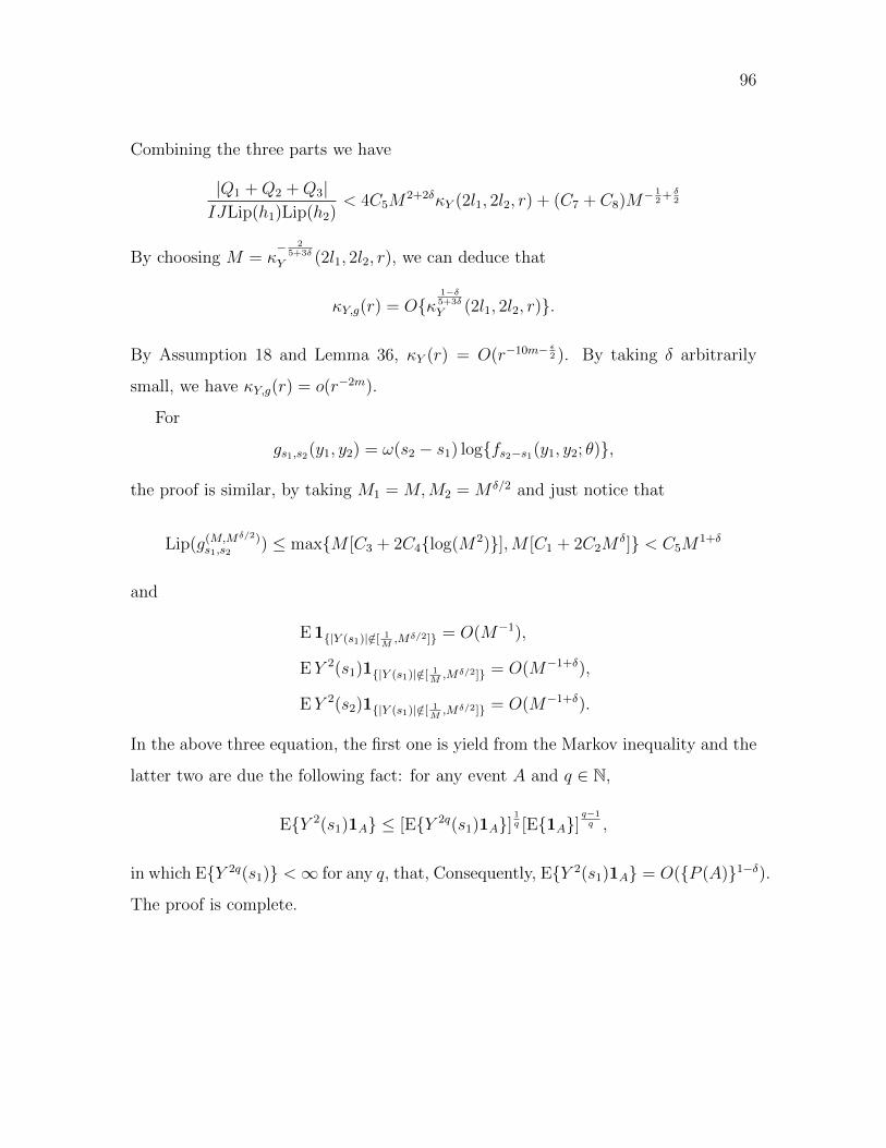
96
Combining the three parts we have
|Q1 +Q2 +Q3|IJLip(h1)Lip(h2)
< 4C5M2+2δκY (2l1, 2l2, r) + (C7 + C8)M− 1
2+ δ
2
By choosing M = κ− 2
5+3δ
Y (2l1, 2l2, r), we can deduce that
κY,g(r) = Oκ1−δ5+3δ
Y (2l1, 2l2, r).
By Assumption 18 and Lemma 36, κY (r) = O(r−10m− ε2 ). By taking δ arbitrarily
small, we have κY,g(r) = o(r−2m).
For
gs1,s2(y1, y2) = ω(s2 − s1) logfs2−s1(y1, y2; θ),
the proof is similar, by taking M1 = M,M2 = M δ/2 and just notice that
Lip(g(M,Mδ/2)s1,s2
) ≤ maxM [C3 + 2C4log(M2)],M [C1 + 2C2Mδ] < C5M
1+δ
and
E 1|Y (s1)|/∈[ 1M,Mδ/2] = O(M−1),
EY 2(s1)1|Y (s1)|/∈[ 1M,Mδ/2] = O(M−1+δ),
EY 2(s2)1|Y (s1)|/∈[ 1M,Mδ/2] = O(M−1+δ).
In the above three equation, the first one is yield from the Markov inequality and the
latter two are due the following fact: for any event A and q ∈ N,
EY 2(s1)1A ≤ [EY 2q(s1)1A]1q [E1A]
q−1q ,
in which EY 2q(s1) <∞ for any q, that, Consequently, EY 2(s1)1A = O(P (A)1−δ).
The proof is complete.
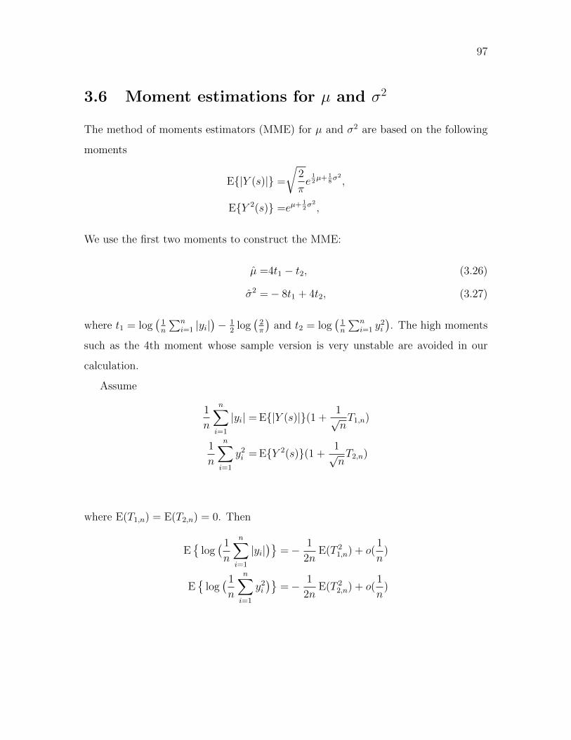
97
3.6 Moment estimations for µ and σ2
The method of moments estimators (MME) for µ and σ2 are based on the following
moments
E|Y (s)| =
√2
πe
12µ+ 1
8σ2
,
EY 2(s) =eµ+ 12σ2
,
We use the first two moments to construct the MME:
µ =4t1 − t2, (3.26)
σ2 =− 8t1 + 4t2, (3.27)
where t1 = log(
1n
∑ni=1 |yi|
)− 1
2log(
2π
)and t2 = log
(1n
∑ni=1 y
2i
). The high moments
such as the 4th moment whose sample version is very unstable are avoided in our
calculation.
Assume
1
n
n∑i=1
|yi| = E|Y (s)|(1 +1√nT1,n)
1
n
n∑i=1
y2i = EY 2(s)(1 +
1√nT2,n)
where E(T1,n) = E(T2,n) = 0. Then
E
log( 1
n
n∑i=1
|yi|)
=− 1
2nE(T 2
1,n) + o(1
n)
E
log( 1
n
n∑i=1
y2i
)=− 1
2nE(T 2
2,n) + o(1
n)
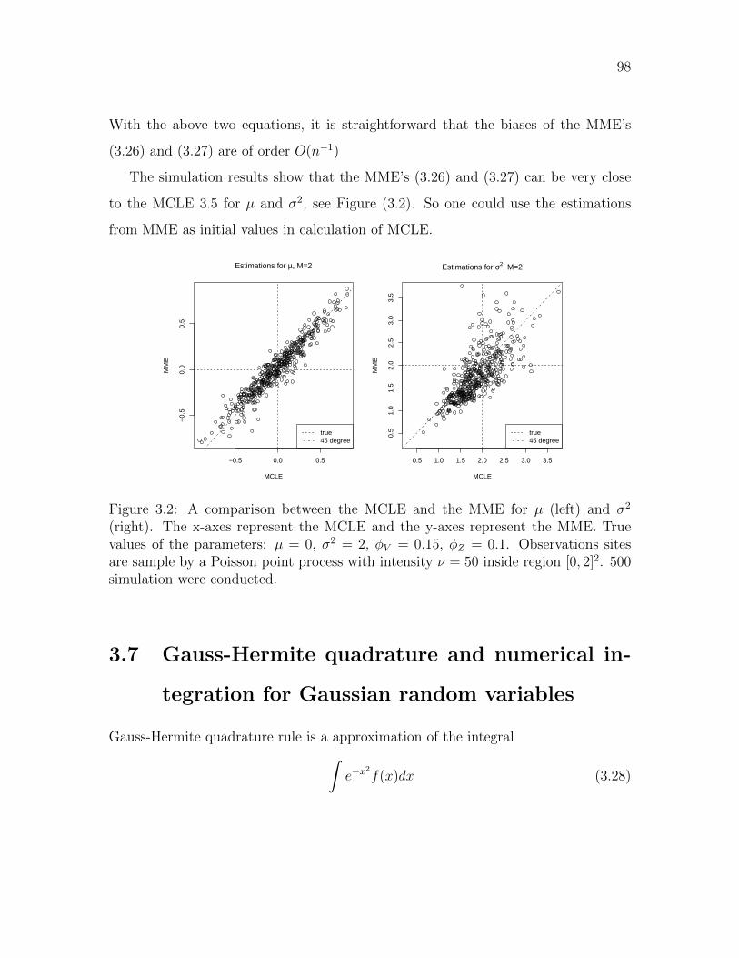
98
With the above two equations, it is straightforward that the biases of the MME’s
(3.26) and (3.27) are of order O(n−1)
The simulation results show that the MME’s (3.26) and (3.27) can be very close
to the MCLE 3.5 for µ and σ2, see Figure (3.2). So one could use the estimations
from MME as initial values in calculation of MCLE.
−0.5 0.0 0.5
−0.
50.
00.
5
Estimations for µ, M=2
MCLE
MM
E
true45 degree
0.5 1.0 1.5 2.0 2.5 3.0 3.5
0.5
1.0
1.5
2.0
2.5
3.0
3.5
Estimations for σ2, M=2
MCLE
MM
E
true45 degree
Figure 3.2: A comparison between the MCLE and the MME for µ (left) and σ2
(right). The x-axes represent the MCLE and the y-axes represent the MME. Truevalues of the parameters: µ = 0, σ2 = 2, φV = 0.15, φZ = 0.1. Observations sitesare sample by a Poisson point process with intensity ν = 50 inside region [0, 2]2. 500simulation were conducted.
3.7 Gauss-Hermite quadrature and numerical in-
tegration for Gaussian random variables
Gauss-Hermite quadrature rule is a approximation of the integral∫e−x
2
f(x)dx (3.28)
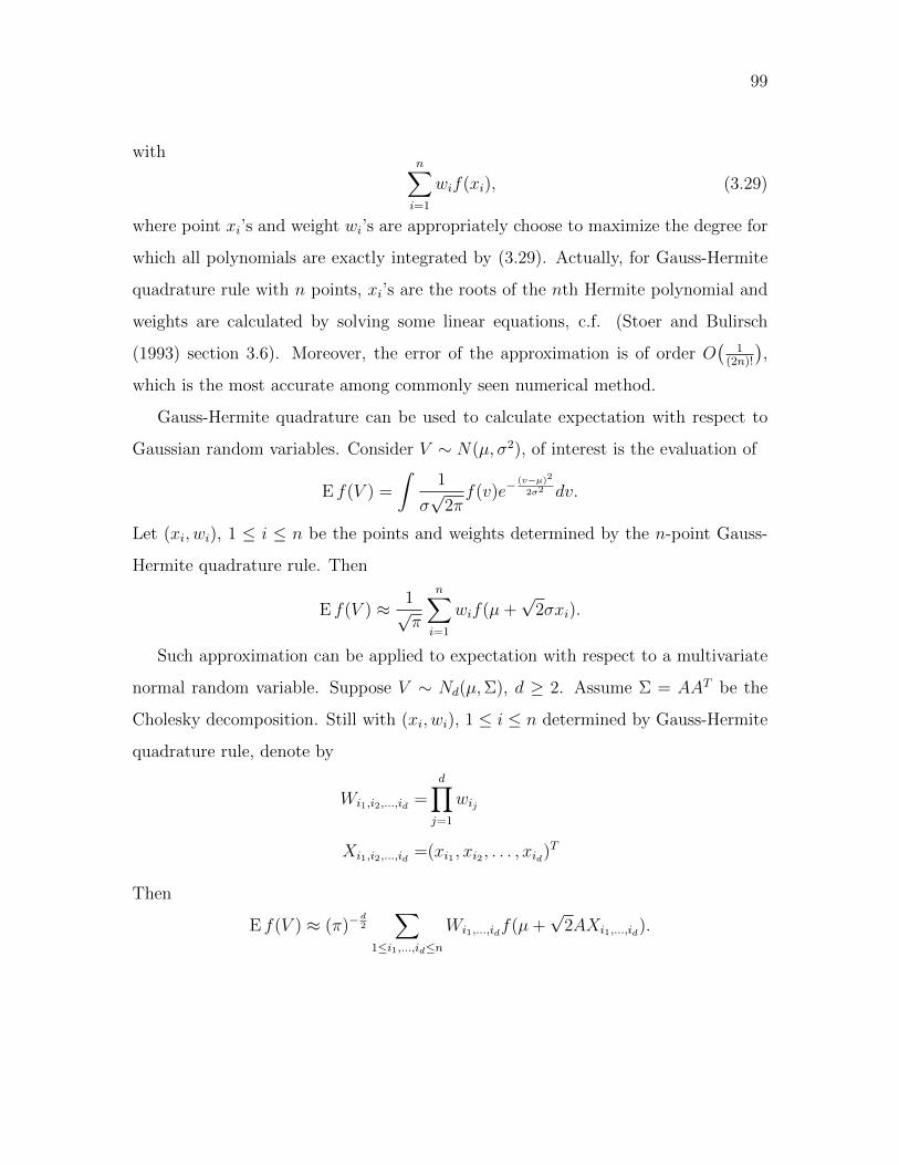
99
withn∑i=1
wif(xi), (3.29)
where point xi’s and weight wi’s are appropriately choose to maximize the degree for
which all polynomials are exactly integrated by (3.29). Actually, for Gauss-Hermite
quadrature rule with n points, xi’s are the roots of the nth Hermite polynomial and
weights are calculated by solving some linear equations, c.f. (Stoer and Bulirsch
(1993) section 3.6). Moreover, the error of the approximation is of order O(
1(2n)!
),
which is the most accurate among commonly seen numerical method.
Gauss-Hermite quadrature can be used to calculate expectation with respect to
Gaussian random variables. Consider V ∼ N(µ, σ2), of interest is the evaluation of
E f(V ) =
∫1
σ√
2πf(v)e−
(v−µ)2
2σ2 dv.
Let (xi, wi), 1 ≤ i ≤ n be the points and weights determined by the n-point Gauss-
Hermite quadrature rule. Then
E f(V ) ≈ 1√π
n∑i=1
wif(µ+√
2σxi).
Such approximation can be applied to expectation with respect to a multivariate
normal random variable. Suppose V ∼ Nd(µ,Σ), d ≥ 2. Assume Σ = AAT be the
Cholesky decomposition. Still with (xi, wi), 1 ≤ i ≤ n determined by Gauss-Hermite
quadrature rule, denote by
Wi1,i2,...,id =d∏j=1
wij
Xi1,i2,...,id =(xi1 , xi2 , . . . , xid)T
Then
E f(V ) ≈ (π)−d2
∑1≤i1,...,id≤n
Wi1,...,idf(µ+√
2AXi1,...,id).

100
3.8 The score function of the bivariate Gaussian
random variables
Suppose (Y1, Y2)T is bivariate Gaussian with mean (0, 0) and covariance matrix 1 ρ
ρ 1
.Then the likelihood function for (Y1, Y2) = (y1, y2) is
f(y1, y2; ρ) =1
2π√
1− ρ2exp
− y2
1 + y22 − 2ρy1y2
2(1− ρ2)
.
The log-likelihood is
log f = − log(2π)− 1
2log(1− ρ2)− y2
1 + y22 − 2ρy1y2
2(1− ρ2),
and the score function is
d log f
dρ= − ρ
(1− ρ2)2(y2
1 + y22 − 2ρy1y2) +
1
1− ρ2y1y2 +
ρ
1− ρ2.
It is straight-forward to verify that E(d log fdρ
)= 0. Now we calculate the second
moment of the score function. Use the representation Y2 = ρY1 +√
1− ρ2Z where
Z ∼ N(0, 1), it follows that
d log f
dρ=− ρ
1− ρ2(Y 2
1 + Z2) +1
1− ρ2(ρY 2
1 +√
1− ρ2Y1Z) +ρ
1− ρ2
=1
1− ρ2
[ρ(1− Z2) +
√1− ρ2Y1Z
]Therefore E
(d log fdρ
)2= 1+ρ2
(1−ρ2)2.
101
Chapter 4
The Convergence Rate and
Asymptotic Distribution of
Bootstrap Quantile Variance
Estimator for Importance
Sampling
1
1This work is first published in Advances in Applied Probability, Vol.44 No.3 c©2012 by TheApplied Probability Trust; see Liu and Yang (2012).
102
4.1 Introduction
In this chapter, we derive the asymptotic distributions of the bootstrap quantile
variance estimators for weighted samples. Let F be a cumulative distribution function
(c.d.f.), f be its density function, and αp = infx : F (x) ≥ p be its p-th quantile.
It is well known that the asymptotic variance of the p-th sample quantile is inversely
proportional to f(αp) (c.f. Bahadur (1966)). When f(αp) is close to zero (e.g. p is
close to zero or one), the sample quantile becomes very unstable since the “effective
samples” size is small. In the scenario of Monte Carlo, one solution is using importance
sampling for variance reduction by distributing more samples around a neighborhood
of the interesting quantile αp. Such a technique has been widely employed in multiple
disciplines. In portfolio risk management, the p-th quantile of a portfolio’s total asset
price is an important risk measure. This quantile is also known as the value-at-risk.
Typically, the probability p in this context is very close to zero (or one). A partial
list of literature of using importance sampling to compute the value-at-risk includes
Glasserman et al. (1999, 2000); Glasserman and Li (2005); Sun and Hong (2009, 2010);
Wang et al. (2009). A recent work by Hult and Svensson (2009) discussed efficient
importance sampling for risk measure computation for heavy-tailed distributions. In
the system stability assessment of engineering, the extreme quantile evaluation is of
interest. In this context, the interesting probabilities are typically of a smaller order
than those of the portfolio risk analysis.
Upon considering p being close to zero or one, the computation of αp can be
viewed as the inverse problem of rare-event simulation. The task of the latter topic
is computing the tail probabilities 1 − F (b) when b tends to infinity. Similar to the
usage in the quantile estimation, importance sampling is also a standard variance
reduction technique for rare-event simulation. The first work on this topic is given by
103
Siegmund (1976), which not only presents an efficient importance sampling estimator
but also defines a second-moment-based efficiency measure. We will later see that
such a measure is also closely related to the asymptotic variance of the weighted
quantiles. Such a connection allows people to adapt the efficient algorithms designed
for rare-event simulations to the computation of quantiles (c.f. Glasserman et al.
(2002); Hult and Svensson (2009)). More recent works of rare-event simulations for
light-tailed distributions include Dupuis and Wang (2005); Sadowsky (1996); Dupuis
and a H. Wang (2007) and for heavy-tailed distributions include Asmussen et al.
(2000); Asmussen and Kroese (2006); Dupuis et al. (2007); Juneja and Shahabuddin
(2002); Blanchet and Glynn (2008); Blanchet et al. (2007a); Blanchet and Liu (2008,
2010). There are also standard textbooks such as Bucklew (2004); Asmussen and
Glynn (2007).
The estimation of distribution quantile is a classic topic. The almost sure result
of sample quantile is established by Bahadur (1966). The asymptotic distribution
of (unweighted) sample quantile can be found in standard textbook such as David
and Nagaraja (2003). Estimation of the (unweighted) sample quantile variance via
bootstrap was proposed by Maritz and Jarrett (1978); McKean and Schrader (1984);
Sheather (1986); Babu (1986); Ghosh et al. (1985). There are also other kernel based
estimators (to estimate f(αp)) for such variances (c.f. Falk (1986)).
There are several pieces of works immediately related to the current one. The
first one is Hall and Martin (1988), which derived the asymptotic distribution of the
bootstrap quantile variance estimator for unweighted i.i.d. samples. Another one is
given by Glynn (1996) who derived the asymptotic distribution of weighted quantile
estimators; see also Chu and Nakayama (2010) for a confidence interval construction.
A more detailed discussion of these results is given in Section 4.2.2.
The asymptotic variance of weighted sample quantile, as reported in Glynn (1996),
104
contains the density function f(αp), whose evaluation typically consists of computa-
tion of high dimensional convolutions and therefore is usually not straightforward. In
this chapter, we propose to use bootstrap method to compute/estimate the variance
of such a weighted quantile. Bootstrap is a generic method that is easy to implement
and does not consist of tuning parameters in contrast to the kernel based methods for
estimating f(αp). This chapter derives the convergence rate and asymptotic distri-
bution of the bootstrap variance estimator for weighted quantiles. More specifically,
the main contributions are to first provide conditions under which the quantiles of
weighted samples have finite variances and develop their asymptotic approximations.
Second, we derive the asymptotic distribution of the bootstrap estimators for such
variances. Let n denote the sample size. Under regularity conditions (for instance,
moment conditions and continuity conditions for the density functions), we show that
the bootstrap variance estimator is asymptotically normal with a convergence rate of
order O(n−5/4). Given that the quantile variance decays at the rate of O(n−1), the
relative standard deviation of a bootstrap estimator is O(n−1/4). Lastly, we present
the asymptotic distribution of the bootstrap estimator for one particular case where
p→ 0.
The technical challenge lies in that many classic results of order statistics are not
applicable. This is mainly caused by the variations introduced by the weights, which
in the current context is the Radon-Nikodym derivative, and the weighted sample
quantile does not map directly to the ordered statistics. In this chapter, we employed
Edgeworth expansion combined with the strong approximation of empirical processes
(Komlos et al. (1975a)) to derive the results.
This chapter is organized as follows. In Section 4.2, we present our main results
and summarize the related results in literature. A numerical implementation is given
in Section 4.3 to illustrate the performance of the bootstrap estimator. The proofs of

105
the theorems are provided in Sections 4.4, 4.5, and 4.6.
4.2 Main results
4.2.1 Problem setting
Consider a probability space (Ω,F , P ) and a random variable X admitting cumulative
distribution function (c.d.f.) F (x) = P (X ≤ x) and density function
f(x) = F ′(x)
for all x ∈ R. Let αp be its p-th quantile, that is,
αp = infx : F (x) ≥ p.
Consider a change of measure Q, under which X admits a cumulative distribution
function G(x) = Q(X ≤ x) and density
g(x) = G′(x).
Let
L(x) =f(x)
g(x),
and X1,...,Xn be i.i.d. copies of X under Q. Assume that P and Q are absolutely con-
tinuous with respect to each other, then EQL(Xi) = 1. The corresponding weighted
empirical c.d.f. is
FX(x) =
∑ni=1 L(Xi)I(Xi ≤ x)∑n
i=1 L(Xi). (4.1)
A natural estimator of αp is
αp(X) = infx ∈ R : FX(x) ≥ p. (4.2)
106
Of interest in this chapter is the variance of αp(X) under the sampling distribution
of Xi, that is
σ2n = V arQ(αp(X)). (4.3)
The notations EQ(·) and V arQ(·) are used to denote the expectation and variance
under measure Q.
Let Y1, ..., Yn be i.i.d. bootstrap samples from the empirical distribution
G(x) =1
n
n∑i=1
I(Xi ≤ x).
The bootstrap estimator for σ2n in (4.3) is defined as
σ2n =
n∑i=1
Q (αp(Y) = Xi) (Xi − αp(X))2, (4.4)
where Y = (Y1, ..., Yn) and Q is the measure induced by G, that is, under Q Y1, ..., Yn
are i.i.d. following empirical distribution G. Note that both G and Q depend on X.
To simplify the notations, we do not include the index of X in the notations of Q and
G.
Remark 5 There are multiple ways to form an estimate of F . One alternative to
(4.1) is
FX(x) =1
n
n∑i=1
L(Xi)I(Xi ≤ x). (4.5)
The analysis of FX is analogous to and simpler than that of (4.1). This is because
the denominator is a constant. The weighted sample c.d.f. in (4.5) only depends
on samples below x. This is an important feature for variance reduction of extreme
quantile estimation when the change of measure Q is designed to be concentrated on
the region below F−1(p). We will provide more detailed discussions later.
107
4.2.2 Related results
In this section, we present two related results in the literature. First, Hall and Martin
(1988) established asymptotic distribution of the the bootstrap variance estimators
for the (unweighted) sample quantiles. In particular, it showed that if the density
function f(x) is Holder continuous with index 12
+ δ0 then
n5/4(σ2n − σ2
n)⇒ N(0, 2π−1/2[p(1− p)]3/2f(αp)−4) (4.6)
as n → ∞. This is consistent with the results in Theorem 42 by setting L(x) ≡ 1.
This chapter can be viewed as a natural extension of Hall and Martin (1988), though
the proof techniques are different.
In the context of importance sampling, as shown by Glynn (1996), if EQ|L(x)|3 <
∞, the asymptotic distribution of a weighted quantile is
√n(αp(X)− αp)⇒ N
(0,V arQ(Wp)
f(αp)2
)(4.7)
as n → ∞, where Wp = L(X)(I(X < αp) − p). More general results in terms of
weighted empirical processes are given by Hult and Svensson (2009).
We now provide a brief discussion on the efficient quantile computation via im-
portance sampling. The sample quantile admits a large variance when f(αp) is small.
One typical situation is that p is very close to zero or one. To fix ideas, we consider
the case where p tends to zero. The asymptotic variance of the p-th quantile of n
i.i.d. samples is1− pnp
p2
f(αp)2.
Then, in order to obtain an estimate of an ε error with at least 1 − δ probability,
the necessary number of i.i.d. samples is proportional to p−1 p2
f2(αp)which grows to
infinity as p→ 0. Typically, the inverse of the hazard function, p/f(αp), varies slowly

108
as p tends to zero. For instance, p/f(αp) is bounded if X is a light-tailed random
variable and grows at the most linearly in αp for most heavy-tailed distributions (e.g.
regularly varying distribution, log-normal distribution).
The asymptotic variance of the quantiles of FX defined in (4.5) is
V arQ(L(X)I(X ≤ αp))
np2
p2
f(αp)2.
There is a wealth of literature on the design of importance sampling algorithms par-
ticularly adapted to the context in which p is close to zero. A well accepted efficien-
cy measure is precisely based on the relative variance p−2V arQ(L(X)I(X ≤ αp))
as p → 0. More precisely, the change of measure is called strongly efficient, if
p−2V arQ(L(X)I(X ≤ αp)) is bounded for arbitrarily small p. A partial list of recent
developments of importance sampling algorithms in the rare event setting includes
Adler et al. (2012); Blachet (2009); Blanchet and Liu (2008); Blanchet et al. (2007b);
Dupuis and Wang (2005). Therefore, the change of measure designed to estimate p
can be adapted without much additional effort to the quantile estimation problem.
For a more thorough discussion, see Hult and Svensson (2009); Chu and Nakayama
(2010). We will provide the analysis of one special in Theorem 43.
4.2.3 The results for regular quantiles
In this subsection, we provide an asymptotic approximation of σ2n and the asymptotic
distribution of σ2n. We first list a set of conditions which we will refer to in the
statements of our theorems.
A1 There exists an α > 4 such that
EQ|L(X)|α <∞.
109
A2 There exists a β > 3 such that
EQ|X|β <∞.
A3 Assume thatα
3>β + 2
β − 3.
A4 There exists a δ0 > 0 such that the density functions f(x) and g(x) are Holder
continuous with index 12
+ δ0 in a neighborhood of αp, that is, there exists a
constant c such that
|f(x)− f(y)| ≤ c|x− y|12
+δ0 , |g(x)− g(y)| ≤ c|x− y|12
+δ0 ,
for all x and y in a neighborhood of αp.
A5 The measures P and Q are absolutely continuous with respect to each other.
The likelihood ratio L(x) ∈ (0,∞) is Lipschitz continuous in a neighborhood of
αp.
A6 Assume f(αp) > 0.
Theorem 41 Let F and G be the cumulative distribution functions of a random
variable X under probability measures P and Q respectively. The distributions F and
G have density functions f(x) = F ′(x) and g(x) = G′(x). We assume that conditions
A1 - A6 hold. Let
Wp = L(X)I(X ≤ αp)− pL(X),
and αp(X) be as defined in (4.2). Then,
σ2n
4= V arQ(αp(X)) =
V arQ(Wp)
nf(αp)2+ o(n−5/4), EQ(αp(X)) = αp + o(n−3/4)
as n→∞.
110
Theorem 42 Suppose that the conditions in Theorem 41 hold and L(X) has density
under Q. Let σ2n be defined as in (4.4). Then, under Q
n5/4(σ2n − σ2
n)⇒ N(0, τ 2p ) (4.8)
as n→∞, where “⇒” denotes weak convergence and
τ 2p = 2π−1/2L(αp)f(αp)
−4(V arQ(Wp))3/2.
Remark 6 In Theorem 41, we provide bounds on the errors of the asymptotic ap-
proximations for EQ(αp(X)) and σ2n in order to assist the analysis of the bootstrap es-
timator. In particular, in order to approximate σ2n with an accuracy of order o(n−5/4),
it is sufficient to approximate EQ(αp(X)) with an accuracy of order o(n−5/8). Thus,
Theorem 41 indicates that αp can be viewed as asymptotically unbiased. In addition,
given that the bootstrap estimator has a convergence rate of Op(n−5/4), Theorem 41
suggests that when computing the distribution of the bootstrap estimator, we can use
the approximation of σ2n to replace the true variance.
In Theorem 42, if we let L(x) ≡ 1, that is, P = Q, then αp is the regular quantile
and the asymptotic distribution (4.8) recovers the result of Hall and Martin (1988)
given in (4.6).
Remark 7 Note that the weak convergence in (4.7) requires weaker conditions than
those in Theorems 41 and 42. The weak convergence does not require αp(X) to have
a finite variance. In contrast, in order to apply the bootstrap variance estimator, one
needs to have the estimand well defined, that is, V arQ(αp(X)) <∞. Conditions A1-3
are imposed to insure that αp(X) has a finite variance under Q.
The continuity assumptions on the density function f and the likelihood ratio
function L (conditions A4 and A5) are typically satisfied in practice. Condition A6
is necessary for the quantile to have a variance of order O(n−1).
111
4.2.4 Results for extreme quantile estimation
In this subsection, we consider one particular scenario when p tends to zero. The
analysis in the context of extreme quantile is sensitive to the underlying distribution
and the choice of change of measure. Here, we only consider a stylized case, one of the
first two cases considered in the rare-event simulation literature. Let X =∑m
j=1 Zi
where Zi’s are i.i.d. random variables with mean zero and density function h(z). The
random variable X has density function f(x) that is the m-th convolution of h(z).
Note that both X and f(x) depend on m. To simplify notation, we omit the index m
when there is no ambiguity. We further consider the exponential change of measure
Q(X ∈ dx) = eθx−mϕ(θ)f(x)dx,
where ϕ(θ) = log∫eθxh(x)dx. We say ϕ is steep if, for every a, ϕ(θ) = a has a
solution. For ε > 0, let αp = −mε be in the large deviations regime. We let θ be
the solution to supθ′(−θ′ε− ϕ(θ′)) and I = supθ′(−θ′ε− ϕ(θ′)). Then, a well known
approximation of the tail probability is given by
P (X < −mε) =c(θ) + o(1)√
me−mI ,
as m→∞. The likelihood ratio is given by
LR(x) = e−θx+mϕ(θ).
We use the notation “LR(x)” to make a difference from the previous likelihood ratio
denoted by “L(x)”.
Theorem 43 Suppose that X =∑m
j=1 Zi, where Zi’s are i.i.d mean-zero random
variable’s with Lipschitz continuous density function. The log-MGF ϕ(θ) is steep.
For ε > 0, equation
ϕ′(θ) = −ε
112
has one solution denoted by θ. Let αp = −mε and X1, ..., Xm be i.i.d. samples
generated from exponential change of measure
Q(X ∈ dx) = eθx−mϕ(θ)f(x).
Let
FX(x) =1
n
n∑i=1
LR(Xi)I(Xi ≤ x), αp(X) = inf(x ∈ R : FX(x) ≥ p). (4.9)
Let Y1, ..., Yn be i.i.d. samples from the empirical measure Q and σ2n be as defined
in (4.4). If m (growing as a function of n and denoted by mn) admits the limit
m3n/n→ c∗ ∈ [0,+∞) as n→∞, then
n5/4
τp(σ2
n − σ2n)⇒ N(0, 1) (4.10)
as n→∞, where σ2n = V arQ(αp(X))
τ 2p = 2π−1/2LR(αp)f(αp)
−4(V arQ(Wp))3/2, Wp = LR(X)I(X ≤ αp).
Remark 8 The above theorem establishes the asymptotic distribution of the bootstrap
variance estimator for a very stylized rare-event simulation problem. For more general
situations, further investigations are necessary, such as the heavy-tailed cases where
the likelihood ratios do not behave as well as those of the lighted cases even for strongly
efficient estimators.
Remark 9 To simplify the notations, we drop the subscript of n in the notation of
mn and write m whenever there is no ambiguity.
As m tends to infinity, the term τ 2p is no longer a constant. With the standard
large deviations results (e.g. Lemma 49 stated later in the proof), we have that τ 2p is
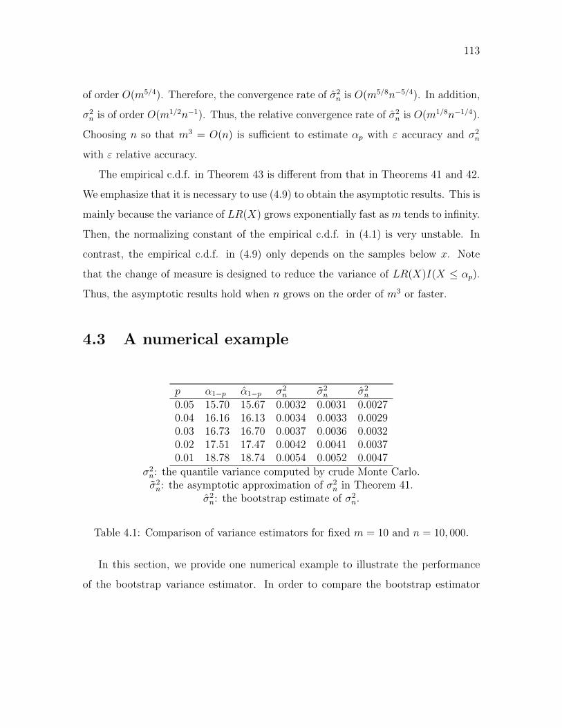
113
of order O(m5/4). Therefore, the convergence rate of σ2n is O(m5/8n−5/4). In addition,
σ2n is of order O(m1/2n−1). Thus, the relative convergence rate of σ2
n is O(m1/8n−1/4).
Choosing n so that m3 = O(n) is sufficient to estimate αp with ε accuracy and σ2n
with ε relative accuracy.
The empirical c.d.f. in Theorem 43 is different from that in Theorems 41 and 42.
We emphasize that it is necessary to use (4.9) to obtain the asymptotic results. This is
mainly because the variance of LR(X) grows exponentially fast as m tends to infinity.
Then, the normalizing constant of the empirical c.d.f. in (4.1) is very unstable. In
contrast, the empirical c.d.f. in (4.9) only depends on the samples below x. Note
that the change of measure is designed to reduce the variance of LR(X)I(X ≤ αp).
Thus, the asymptotic results hold when n grows on the order of m3 or faster.
4.3 A numerical example
p α1−p α1−p σ2n σ2
n σ2n
0.05 15.70 15.67 0.0032 0.0031 0.00270.04 16.16 16.13 0.0034 0.0033 0.00290.03 16.73 16.70 0.0037 0.0036 0.00320.02 17.51 17.47 0.0042 0.0041 0.00370.01 18.78 18.74 0.0054 0.0052 0.0047
σ2n: the quantile variance computed by crude Monte Carlo.σ2n: the asymptotic approximation of σ2
n in Theorem 41.σ2n: the bootstrap estimate of σ2
n.
Table 4.1: Comparison of variance estimators for fixed m = 10 and n = 10, 000.
In this section, we provide one numerical example to illustrate the performance
of the bootstrap variance estimator. In order to compare the bootstrap estimator

114
m p α1−p α1−p σ2n σ2
n σ2n
10 7.0e-02 15 14.95 1.1e-03 1.0e-03 1.2e-0330 7.3e-03 45 44.95 2.2e-03 2.2e-03 1.7e-0350 9.0e-04 75 74.98 3.0e-03 3.2e-03 2.4e-03100 5.9e-06 150 149.99 4.8e-03 4.9e-03 5.0e-03
Table 4.2: Comparison of variance estimators as m→∞, αp = 1.5m, and n = 10, 000.
with the asymptotic approximation in Theorem 41, we choose an example for which
the marginal density f(x) is in a closed form and αp can be computed numerically.
Consider a partial sum
X =m∑i=1
Zi
where Zi’s are i.i.d. exponential random variables with rate one. Then, the density
function of X is
f(x) =xm−1
(m− 1)!e−x.
We are interested in computing X’s (1 − p)-th quantile via exponential change of
measure that isdQθ
dP=
m∏i=1
eθZi−ϕ(θ), (4.11)
where ϕ(θ) = − log(1− θ) for θ < 1. We further choose θ = arg supθ′(θ′αp−mϕ(θ′)).
We generate n i.i.d. replicates of (Z1, ..., Zm) from Qθ, that is, (Z(k)1 , ..., Z
(k)m ) for
k = 1, ..., n; then, use Xk =∑m
i=1 Z(k)i , k = 1, ..., n and the associated weights to
form an empirical distribution and further α1−p(X). Let σ2n = V arQθ(α1−p(X)), σ2
n
be the asymptotic approximation of σ2n, and σ2
n be the bootstrap estimator of σ2n. We
use Monte Carlo to compute both σ2n and σ2
n by generating independent replicates of
α1−p(X) under Q and bootstrap samples under Q respectively.
We first consider the situation when m = 10. Table 4.1 shows the results using

115
the estimators based on the empirical c.d.f. in Theorem 42 with n = 10, 000. In the
table, the column σ2n shows the variances of α1−p estimated using 1000 Monte Carlo
simulations. In addition, we consider the case that αp = 1.5m and send m to infinity.
Table 4.2 shows the numerical results using the estimators in Theorem 43 based on
n = 10, 000 simulations.
4.4 Proof of Theorem 41
Throughout our discussion we use the following notations for asymptotic behavior.
We say that 0 ≤ g(b) = O(h(b)) if g(b) ≤ ch(b) for some constant c ∈ (0,∞) and
all b ≥ b0 > 0. Similarly, g(b) = Ω(h(b)) if g(b) ≥ ch(b) for all b ≥ b0 > 0. We also
write g(b) = Θ(h(b)) if g(b) = O(h(b)) and g(b) = Ω(h(b)). Finally, g(b) = o(h(b)) as
b→∞ if g(b)/h(b)→ 0 as b→∞.
Before the proof of Theorem 41, we first present a few useful lemmas.
Lemma 44 X is random variable with finite second moment, then
EX =
∫x>0
P (X > x)dx−∫x<0
P (X < x)dx
EX2 =
∫x>0
2xP (X > x)dx−∫x<0
2xP (X < x)dx
Lemma 45 Let X1, ..., Xn be i.i.d. random variables with EXi = 0 and E|Xi|α <∞
for some α > 2. For each ε > 0, there exists a constant κ depending on ε, EX2i and
E|Xi|α such that
E
∣∣∣∣∣n∑i=1
Xi/√n
∣∣∣∣∣α−ε
≤ κ
for all n > 0.
The proofs of Lemmas 44 and 45 are elementary. Therefore, we omit them.
116
Lemma 46 Let h(x) be a non-negative function. There exists ζ0 > 0 such that
h(x) ≤ xζ0 for all x sufficiently large. Then, for all ζ1, ζ2, λ > 0 such that (ζ1− 1)λ <
ζ2, we obtain∫ nλ
0
h(x)Φ(−x+ o(xζ1n−ζ2))dx =
∫ nλ
0
h(x)Φ(−x)dx+ o(n−ζ2),
as n→∞, where Φ is the c.d.f. of a standard Gaussian distribution. In addition, we
write an(x) = o(xζ1n−ζ2) if an(x)x−ζ1nζ2 → 0 as n→∞ uniformly for x ∈ (ε, nλ).
Proof of Lemma 46. We first split the integral into∫ nλ
0
h(x)Φ(−x+ o(xζ1n−ζ2))dx
=
∫ (logn)2
0
h(x)Φ(−x+ o(xζ1n−ζ2))dx+
∫ nλ
(logn)2h(x)Φ(−x+ o(xζ1n−ζ2))dx.
Note that the second term∫ nλ
(logn)2h(x)Φ(−x+ o(xζ1n−ζ2))dx ≤ nλ(ζ0+1)Φ(− (log n)2 /2) = o(n−ζ2).
For the first term, note that for all 0 ≤ x ≤ (log n)2,
Φ(−x+ o(xζ1n−ζ2)) = (1 + o(xζ1+1n−ζ2))Φ(−x).
Then ∫ (logn)2
0
h(x)Φ(−x+ o(xζ1n−ζ2))dx =
∫ (logn)2
0
h(x)Φ(−x)dx+ o(n−ζ2).
Therefore, the conclusion follows immediately.
Proof of Theorem 41. Let αp(X) be defined in (4.2). To simplify the notation,
we omit the index X and write αp(X) as αp. We use Lemma 44 to compute the
117
moments. In particular, we need to approximate the following probability,
Q(n1/2(αp − αp) > x
)= Q(FX(αp + xn−1/2) < p) (4.12)
= Q
(n∑i=1
L(Xi)(I(Xi ≤ αp + xn−1/2)− p
)< 0
).
For some λ ∈ ( 14(α−2)
, 18), we provide approximations for (4.12) of the following three
cases: 0 < x ≤ nλ, nλ ≤ x ≤ c√n, and x >
√n. The development for
Q(n1/2(αp − αp) < x)
on the region that x ≤ 0 is the same as that of the positive side.
Case 1: 0 < x ≤ nλ.
Let
Wx,n,i = L(Xi)(I(Xi ≤ αp + xn−1/2)− p
)− F (αp + xn−1/2) + p.
According to Berry-Esseen bound (c.f. Durrett (2010)),
Q
(n∑i=1
L(Xi)(I(Xi ≤ αp + xn−1/2)− p
)< 0
)
= Q
1n
∑ni=1Wx,n,i√
1nV arQWx,n,1
< −F (αp + xn−1/2)− p√1nV arQWx,n,1
= Φ
− (F (αp + xn−1/2)− p)√
1nV arQWx,n,1
+D1(x). (4.13)
There exists a constant κ1 such that
|D1(x)| ≤ κ1
(V arQWx,n,1)3/2n−1/2.

118
Case 2: nλ ≤ x ≤ c√n.
Thanks to Lemma 45, for each ε > 0, the (α − ε)-th moment of 1√n
∑ni=1Wx,n,i is
bounded. By Chebyshev’s inequality, we obtain that
Q
(n∑i=1
L(Xi)(I(Xi ≤ αp + xn−1/2)− p) < 0
)= Q
(1√n
n∑i=1
Wx,n,i ≤√n(p− F (αp + x/
√n)))
≤ κ1
(1√
n(F (αp + xn−1/2)− p)
)α−ε≤ κ2x
−α+ε.
Since λ > 14(α−2)
, we choose ε small enough such that∫ c√n
nλxQ(αp − αp > xn−1/2)dx = O(n−λ(α−2−ε)) = o(n−1/4). (4.14)
Case 3: x > c√n.
Note that
Q
(n∑i=1
L(Xi)(I(Xi ≤ αp + xn−1/2)− p) < 0
)is a non-increasing function of x. Therefore, for all x > c
√n, from Case 2, we obtain
that
Q
(n∑i=1
L(Xi)(I(Xi ≤ αp + xn−1/2)− p) < 0
)≤ κ2(c
√n)−α+ε = κ3n
−α/2+ε/2.
For c√n < x ≤ nα/6−ε/6, we have that
Q
(n∑i=1
L(Xi)(I(Xi ≤ αp + xn−1/2)− p) < 0
)≤ κ3n
−α/2+ε/2 ≤ κ3x−3.
In addition, note that for all xβ−3 > n1+β/2,
Q(αp > αp + x/
√n)≤ Q(sup
iXi > αp + xn−1/2) = 1−Gn(αp + xn−1/2)
≤ O(1)n1+β/2x−β = O(x−3).
119
Therefore, Q (αp > αp + x/√n) = O(x−3) on the region c
√n < x ≤ nα/6−ε/3∪x >
nβ+2
2(β−3). Since α3> β+2
β−3, one can choose ε small enough such that x > nα/6−ε/6 implies
xβ−3 > n1+β/2. Therefore, for all x > c√n, we obtain that
Q(αp > αp + x/
√n)≤ x−3,
and ∫ ∞c√n
xQ(αp > αp + x/
√n)
= O(n−1/2). (4.15)
A summary of Cases 1, 2, and 3.
Summarizing the Cases 2 and 3, more specifically (4.14) and (4.15), we obtain that∫ ∞nλ
xQ(αp > αp + x/
√n)dx = o(n−1/4).
Using the result in (4.13), we obtain that∫ ∞0
xQ(αp > αp + x/
√n)dx
=
∫ nλ
0
x
Φ
− (F (αp + xn−1/2)− p)√
1nV arQWx,n,1
+O(n−1/2)
dx+ o(n−1/4)
=
∫ nλ
0
xΦ
− (F (αp + xn−1/2)− p)√
1nV arQWx,n,1
dx+O(n2λ−1/2) + o(n−1/4). (4.16)
Given that λ < 18, we have that O(n2λ−1/2) = o(n−1/4). Thanks to condition A4 and
the fact that V arQ(Wx,n,1) = (1 +O(xn−1/2))V arQ(W0,n,1), we have
−(F (αp + xn−1/2)− p
)√1nV arQWx,n,1
= − xf(αp)√V arQW0,n,1
+O(x32
+δ0n−1/4−δ0/2).
Insert this approximation to (4.16). Together with the results from Lemma 46, we
obtain that∫ nλ
0
xQ(αp > αp + x/
√n)dx =
∫ nλ
0
xΦ
(− xf(αp)√
V arQW0,n,1
)dx+ o(n−1/4).
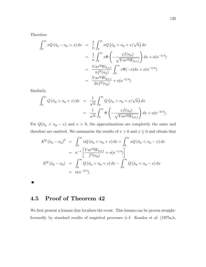
120
Therefore∫ ∞0
xQ (αp − αp > x) dx =1
n
∫ ∞0
xQ(αp > αp + x/
√n)dx
=1
n
∫ ∞0
xΦ
(− xf(αp)√
V arQW0,n,1
)dx+ o(n−5/4)
=V arQW0,n,1
nf 2(αp)
∫ ∞0
xΦ(−x)dx+ o(n−5/4)
=V arQW0,n,1
2nf 2(αp)+ o(n−5/4).
Similarly,∫ ∞0
Q (αp > αp + x) dx =1√n
∫ ∞0
Q(αp > αp + x/
√n)dx
=1√n
∫ ∞0
Φ
(− xf(αp)√
V arQW0,n,1
)dx+ o(n−3/4).
For Q(αp < αp − x) and x > 0, the approximations are completely the same and
therefore are omitted. We summarize the results of x > 0 and x ≤ 0 and obtain that
EQ (αp − αp)2 =
∫ ∞0
xQ (αp > αp + x) dx+
∫ ∞0
xQ (αp < αp − x) dx
= n−1
[V arQW0,n,1
f 2(αp)+ o(n−1/4)
]EQ (αp − αp) =
∫ ∞0
Q (αp > αp + x) dx−∫ ∞
0
Q (αp < αp − x) dx
= o(n−3/4).
4.5 Proof of Theorem 42
We first present a lemma that localizes the event. This lemma can be proven straight-
forwardly by standard results of empirical processes (c.f. Komlos et al. (1975a,b,
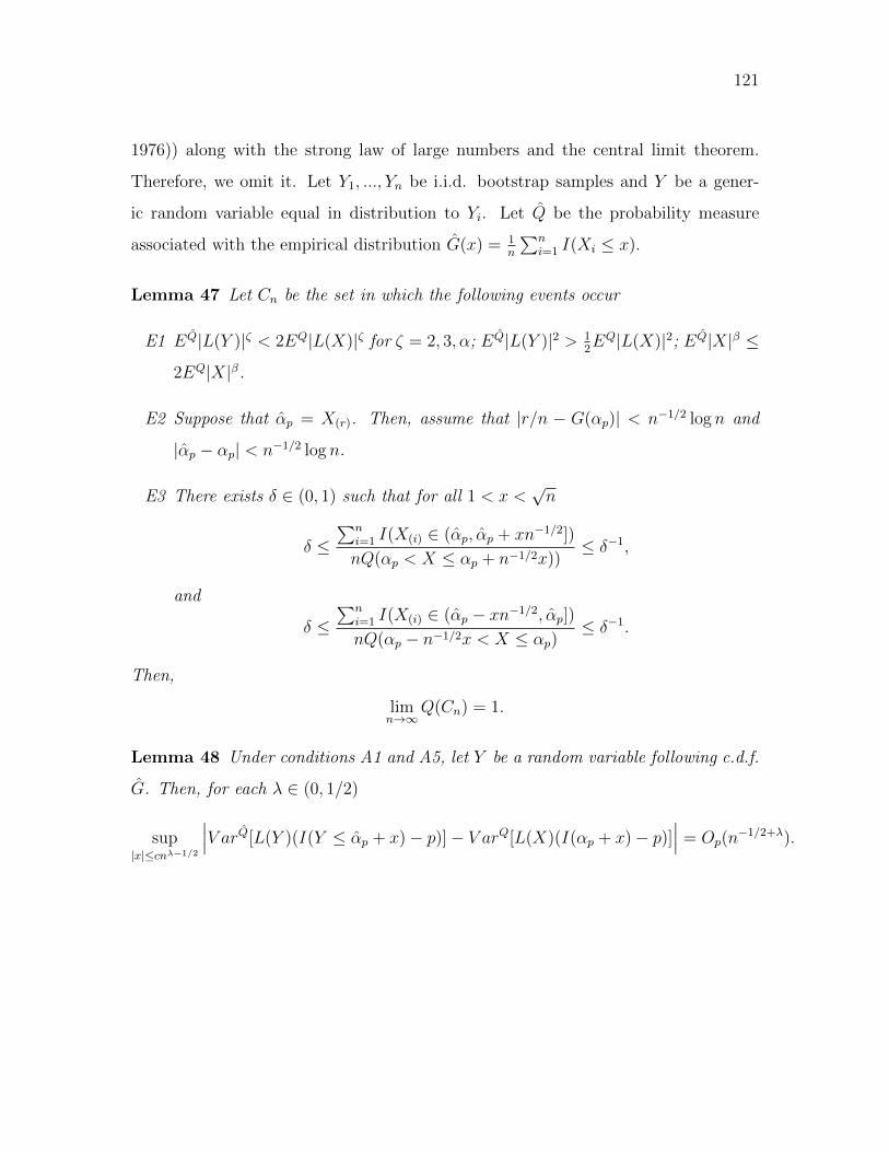
121
1976)) along with the strong law of large numbers and the central limit theorem.
Therefore, we omit it. Let Y1, ..., Yn be i.i.d. bootstrap samples and Y be a gener-
ic random variable equal in distribution to Yi. Let Q be the probability measure
associated with the empirical distribution G(x) = 1n
∑ni=1 I(Xi ≤ x).
Lemma 47 Let Cn be the set in which the following events occur
E1 EQ|L(Y )|ζ < 2EQ|L(X)|ζ for ζ = 2, 3, α; EQ|L(Y )|2 > 12EQ|L(X)|2; EQ|X|β ≤
2EQ|X|β.
E2 Suppose that αp = X(r). Then, assume that |r/n − G(αp)| < n−1/2 log n and
|αp − αp| < n−1/2 log n.
E3 There exists δ ∈ (0, 1) such that for all 1 < x <√n
δ ≤∑n
i=1 I(X(i) ∈ (αp, αp + xn−1/2])
nQ(αp < X ≤ αp + n−1/2x))≤ δ−1,
and
δ ≤∑n
i=1 I(X(i) ∈ (αp − xn−1/2, αp])
nQ(αp − n−1/2x < X ≤ αp)≤ δ−1.
Then,
limn→∞
Q(Cn) = 1.
Lemma 48 Under conditions A1 and A5, let Y be a random variable following c.d.f.
G. Then, for each λ ∈ (0, 1/2)
sup|x|≤cnλ−1/2
∣∣∣V arQ[L(Y )(I(Y ≤ αp + x)− p)]− V arQ[L(X)(I(αp + x)− p)]∣∣∣ = Op(n
−1/2+λ).

122
Proof of Lemma 48. Note that
EQL2(Y )(I(Y ≤ αp + x)− p)2 =1
n
n∑i=1
L2(Xi)(I(Xi ≤ αp + x)− p)2
=1
n
n∑i=1
L2(Xi)(I(Xi ≤ αp + x)− p)2
+L2 (αp)Op
(1
n
n∑i=1
I(min(αp, αp) ≤ Xi − x ≤ max(αp, αp))
).
For the first term, by central limit theorem, continuity of L(x), and Taylor’s expan-
sion, we obtain that
sup|x|≤cn−1/2+λ
∣∣∣∣∣ 1nn∑i=1
L2(Xi)(I(Xi ≤ αp + x)− p)2 − EQ(L2(X)(I(X ≤ αp + x)− p)2
)∣∣∣∣∣ = Op(n−1/2+λ).
Thanks to the weak convergence of empirical measure and αp − αp = O(n−1/2), we
have that the second term
L2 (αp)Op
(1
n
n∑i=1
I(min(αp, αp) ≤ Xi − x ≤ max(αp, αp))
)= Op(n
−1/2).
Therefore,
sup|x|≤cn−1/2+λ
∣∣∣EQL2(Y )(I (Y ≤ αp + x)− p)2 − EQ(L2(X)(I(X ≤ αp + x)− p)2)∣∣∣ = Op(n
−1/2+λ).
With a very similar argument, we have that
sup−cn−1/2≤x≤cn−1/2
∣∣∣EQL(Y )(I (Y ≤ αp + x)− p)− EQ(L(X)(I(X ≤ αp + x)− p))∣∣∣ = Op(n
−1/2+λ).
Thereby, we conclude the proof.
Proof of Theorem 42. Let X(1), ..., X(n) be the order statistics of X1, ..., Xn in
an ascending order. Since we aim at proving weak convergence, it is sufficient to

123
consider the case that X ∈ Cn as in Lemma 47. Throughout the proof, we assume
that X ∈ Cn.
Similar to the notations in the proof of Theorem 41, we write αp(X) as αp and
keep the notation αp(Y) to differentiate them. We use Lemma 44 to compute the
second moment of αp(Y)− αp under Q, that is,
σ2n =
∫ ∞0
xQ(αp(Y) > αp + x)dx+
∫ ∞0
xQ(αp(Y) < αp − x)dx.
We first consider the case that x > 0 and proceed to a similar derivation as that of
Theorem 41. Choose λ ∈ ( 14(α−2)
, 18).
Case 1: 0 < x ≤ nλ.
Similar to the proof of Theorem 41 by Berry-Esseen bound, for all x ∈ R
Q(n1/2(αp(Y)− αp) > x
)= Φ
−∑ni=1 L(Xi)
(I(Xi ≤ αp + xn−1/2)− p
)√nV arQWx,n
+D2,
where
Wx,n = L(Y )(I(Y ≤ αp + xn−1/2)− p
)− 1
n
n∑i=1
L(Xi)(I(Xi ≤ αp + x/
√n)− p
),
and (thanks to E1 in Lemma 47)
|D2| ≤3EQ
∣∣∣Wx,n
∣∣∣3√n(V arQWx,n
)3/2= O(n−1/2).
In what follows, we further consider the cases that x > nλ. We will essentially
follow the Cases 2 and 3 in the proof of Theorem 41.

124
Case 2: nλ ≤ x ≤ c√n.
Note thatn∑i=1
L(Xi) (I(Xi ≤ αp)− p) = O(1).
With exactly the same argument as in Case 2 of Theorem 41 and thanks to E1 in
Lemma 47, we obtain that for each ε > 0
Q(αp(Y)− αp > xn−1/2
)≤ κ
(1√n
n∑i=1
L(Xi)(I(Xi ≤ αp + x/
√n)− p
))−α+ε
= κ
(1√n
n∑i=1
L(Xi)I(αp < Xi ≤ αp + x/√n) +O(1/
√n)
)−α+ε
Further, thanks to E3 in Lemma 47, we have
Q(αp(Y)− αp > xn−1/2
)= O(x−α+ε).
With ε sufficiently small, we have∫ √nnλ
xQ(αp(Y)− αp > xn−1/2
)dx = O(n−λ(α−ε−2)) = o(n−1/4).
Case 3: x > c√n.
Note that
Q
(n∑i=1
L(Yi)(I(Yi ≤ αp + xn−1/2)− p
)< 0
),
is a monotone non-increasing function of x. Therefore, for all x > c√n, from Case 2,
we obtain that
Q
(n∑i=1
L(Yi)(I(Yi ≤ αp + xn−1/2)− p
)< 0
)≤ κ3n
−α/2+ε/2.
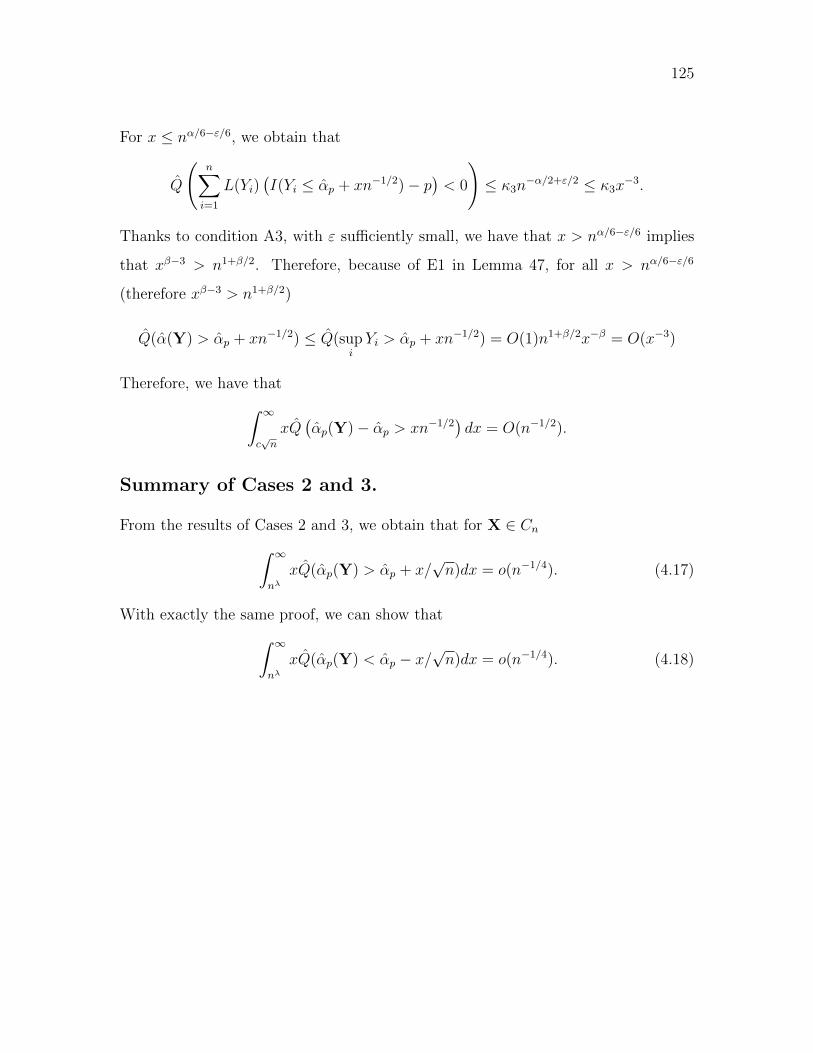
125
For x ≤ nα/6−ε/6, we obtain that
Q
(n∑i=1
L(Yi)(I(Yi ≤ αp + xn−1/2)− p
)< 0
)≤ κ3n
−α/2+ε/2 ≤ κ3x−3.
Thanks to condition A3, with ε sufficiently small, we have that x > nα/6−ε/6 implies
that xβ−3 > n1+β/2. Therefore, because of E1 in Lemma 47, for all x > nα/6−ε/6
(therefore xβ−3 > n1+β/2)
Q(α(Y) > αp + xn−1/2) ≤ Q(supiYi > αp + xn−1/2) = O(1)n1+β/2x−β = O(x−3)
Therefore, we have that∫ ∞c√n
xQ(αp(Y)− αp > xn−1/2
)dx = O(n−1/2).
Summary of Cases 2 and 3.
From the results of Cases 2 and 3, we obtain that for X ∈ Cn∫ ∞nλ
xQ(αp(Y) > αp + x/√n)dx = o(n−1/4). (4.17)
With exactly the same proof, we can show that∫ ∞nλ
xQ(αp(Y) < αp − x/√n)dx = o(n−1/4). (4.18)
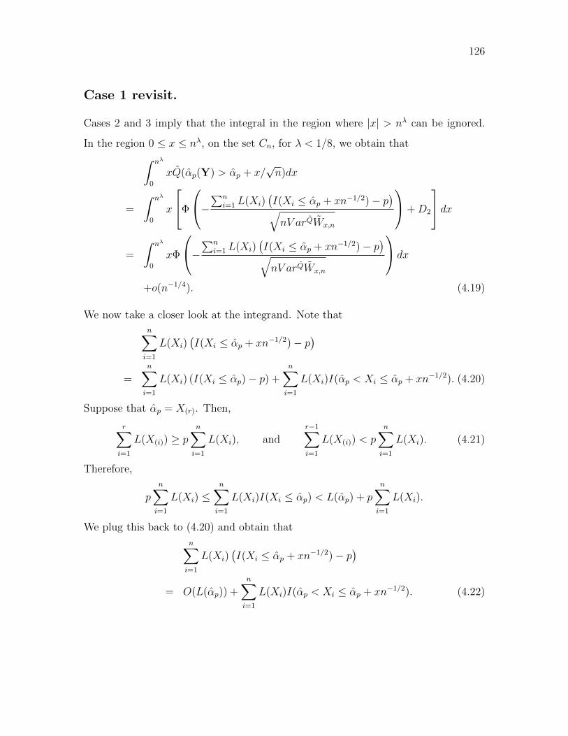
126
Case 1 revisit.
Cases 2 and 3 imply that the integral in the region where |x| > nλ can be ignored.
In the region 0 ≤ x ≤ nλ, on the set Cn, for λ < 1/8, we obtain that∫ nλ
0
xQ(αp(Y) > αp + x/√n)dx
=
∫ nλ
0
x
Φ
−∑ni=1 L(Xi)
(I(Xi ≤ αp + xn−1/2)− p
)√nV arQWx,n
+D2
dx=
∫ nλ
0
xΦ
−∑ni=1 L(Xi)
(I(Xi ≤ αp + xn−1/2)− p
)√nV arQWx,n
dx
+o(n−1/4). (4.19)
We now take a closer look at the integrand. Note that
n∑i=1
L(Xi)(I(Xi ≤ αp + xn−1/2)− p
)=
n∑i=1
L(Xi) (I(Xi ≤ αp)− p) +n∑i=1
L(Xi)I(αp < Xi ≤ αp + xn−1/2). (4.20)
Suppose that αp = X(r). Then,
r∑i=1
L(X(i)) ≥ pn∑i=1
L(Xi), andr−1∑i=1
L(X(i)) < pn∑i=1
L(Xi). (4.21)
Therefore,
p
n∑i=1
L(Xi) ≤n∑i=1
L(Xi)I(Xi ≤ αp) < L(αp) + p
n∑i=1
L(Xi).
We plug this back to (4.20) and obtain that
n∑i=1
L(Xi)(I(Xi ≤ αp + xn−1/2)− p
)= O(L(αp)) +
n∑i=1
L(Xi)I(αp < Xi ≤ αp + xn−1/2). (4.22)
127
In what follows, we study the dominating term in (4.19) via (4.22). For all x ∈
(0, nλ), thanks to (4.22), we obtain that
Φ
−∑ni=1 L(Xi)(I(Xi ≤ αp + xn−1/2)− p)√
nV arQWx,n
= Φ
−∑ni=1 L(Xi)I(αp < Xi ≤ αp + xn−1/2)√
nV arQWx,n
+O(n−1/2)
. (4.23)
Note that the above display is a functional of (X1, ..., Xn) and is also a stochastic
process indexed by x. In what follows we show that it is asymptotically a Gaussian
process. The distribution of (4.23) is not straightforward to obtain. The strategy is
to first consider a slightly different quantity and then connect it to (4.23). For each
(x(r), r) such that |x(r)−αp| ≤ n−1/2 log n and |r/n−G(αp)| ≤ n−1/2 log n, conditional
on X(r) = x(r), X(r+1), ..., X(n) are equal in distribution to the order statistics of (n−r)
i.i.d. samples from Q(X ∈ ·|X > x(r)). Thanks to the fact that L(x) is locally
Lipschitz continuous and E3 in Lemma 47, we obtain
Φ
−∑ni=r+1 L(X(i))I(x(r) < X(i) ≤ x(r) + xn−1/2)√
nV arQWx,n
+O(n−1/2)
(4.24)
= Φ
− L(x(r))√nV arQWx,n
n∑i=r+1
I(X(i) ∈ (x(r), x(r) + xn−1/2]) +O(x2n−1/2)
.
In the above inequality, we replace L(X(i)) by L(X(r)). The error term is
O(1)L′(X(r))xn
−1/2∑n
i=r+1 I(x(r) < X(r) ≤ x(r) + xn−1/2)√nV arQWx,n
= O(x2n−1/2).
Note that the display (4.24) equals to (4.23) if αp = X(r) = x(r). For the time being,
we proceed by conditioning only on X(r) = x(r) and then further derive the conditional
128
distribution of (4.23) given αp = X(r) = x(r). Due to Lemma 48, we further simplify
the denominator and the display (4.24) equals to
Φ
(−
L(x(r))√nV arQW0,n
n∑i=r+1
I(X(i) ∈ (x(r), x(r) + xn−1/2]) +O(x2n−1/2+λ)
). (4.25)
Let
Gx(r)(x) =G(x(r) + x)−G(x(r))
1−G(x(r))= Q(X ≤ x(r) + x|X > x(r)).
Thanks to the result of strong approximation (Komlos et al. (1975a,b, 1976)), given
X(r) = x(r), there exists a Brownian bridge B(t) : t ∈ [0, 1], such that
n∑i=r+1
I(X(i) ∈ (x(r), x(r) + xn−1/2])
= (n− r)Gx(r)(xn−1/2) +
√n− rB(Gx(r)(xn
−1/2)) +Op(log(n− r)), (4.26)
where the Op(log(n− r)) is uniform in x. Again, we can localize the event by consid-
ering a set in which the error term in the above display is O(log(n − r))2. We plug
this strong approximation back to (4.25) and obtain
Φ
(−
L(x(r))√nV arQW0,n
(n− r)Gx(r)(xn−1/2) +Op(x
2n−1/2+λ(log n)2)
)(4.27)
−ϕ
(−
L(x(r))√nV arQW0,n
(n− r)Gx(r)(xn−1/2) +Op(x
2n−1/4(log n)2)
)
×(n− r)1/2L(x(r))√
nV arQW0,n
B(Gx(r)(xn−1/2)).
In addition, thanks to condition A4,
L(x(r))√nV arQW0,n
(n− r)Gx(r)(xn−1/2) =
f(x(r))√V arQW0,n
x+O(xδ0+3/2n−1/4−δ0/2). (4.28)
Let
ξ(x) =(n− r)1/2L(x(r))√
nV arQW0,n
B(Gx(r)(xn−1/2)) (4.29)

129
which is a Gaussian process with mean zero and covariance function
Cov(ξ(x), ξ(y)) =(n− r)L2(x(r))
nV arQW0,n
Gx(r)(x/√n)(1−Gx(r)(y/
√n))
= (1 +O(n−1/4+λ/2))L(x(r))f(x(r))
V arQW0,n
x√n
(4.30)
for 0 ≤ x ≤ y ≤ nλ. Insert (4.28) and (4.29) back to (4.27) and obtain that given
X(r) = x(r)
∫ nλ
0
2xΦ
−∑ni=r+1 L(X(i))I(x(r) < X(i) ≤ x(r) + xn−1/2)√
nV arQWx,n
+O(n−1/2)
dx
=
∫ nλ
0
2xΦ
(−
f(x(r))√V arQW0,n
x+ o(x2n−1/4)
)dx (4.31)
−∫ nλ
0
2xϕ
(−
f(x(r))√V arQW0,n
x+ o(x2n−1/4)
)ξ(x)dx+ o(n−1/4),
where ϕ(x) is the standard Gaussian density function. Due to Lemma 46 and |x(r)−
αp| ≤ n−1/2 log n, the first term on the right side of (4.31) is∫ nλ
0
2xΦ
(−
f(x(r))√V arQW0,n
x+ o(x2n−1/4)
)dx (4.32)
= (1 + o(n−1/4))
∫ ∞0
2xΦ
(− f(αp)√
V arQW0,n
x
)dx+ op(n
−1/4).
The second term on the right side of (4.31) multiplied by n1/4 converges weakly to a

130
Gaussian distribution with mean zero and variance
√n
∫ nλ
0
∫ nλ
0
4xyϕ
(−
f(x(r))√V arQW0,n
x+ o(x2n−1/4)
)
ϕ
(−
f(x(r))√V arQW0,n
y + o(x2n−1/4)
)Cov(ξ(x), ξ(y))dxdy
= (1 + o(1))
∫ nλ
0
∫ nλ
0
4xyϕ
(−
f(x(r))√V arQW0,n
x
)ϕ
(−
f(x(r))√V arQW0,n
y
)
×L(x(r))f(x(r))
V arQW0,n
min(x, y)dxdy
= (1 + o(1))L(αp)
(V arQW0,n
)3/2
f 4(αp)√π
. (4.33)
To obtain the last step of the above display, we need the following calculation
V ar
(∫ ∞0
2xϕ(x)B(x)dx
)=
∫ ∞0
∫ ∞0
4xyϕ(x)ϕ(y) min(x, y)dx
=
∫ ∞0
∫ ∞0
4r3 cos θ sin θmin(cos θ, sin θ)1
2πe−r
2/2dxdy
= 8
∫ π/4
0
∫ ∞0
r4 cos θ sin2 θ1√2π
1√2πe−r
2/2drdθ
= 81
3
1
23/2
1√2π
3
2
=1√π.
We insert the estimates in (4.32) and (4.33) back to (4.31) and obtain that conditional
on X(r) = x(r),
n1/4∫ nλ
0
2xΦ
−∑ni=r+1 L(X(i))I(x(r) < X(i) ≤ x(r) + xn−1/2)√
nV arQWx,n
+O(n−1/2)
dx
−∫ ∞
0
2xΦ
(− f(αp)√
V arQW0,n
x
)dx
=⇒ N(0, τ 2p /2) (4.34)
131
as n−r, r →∞ subject to the constraint that |r/n−G−1(αp)| ≤ n−1/2 log n, where τ 2p
is defined in the statement of the theorem. One may consider that the left-hand-side
of (4.34) is indexed by r and n − r. The limit is in the sense that both r and n − r
tend to infinity in the region that |r/n−G−1(αp)| ≤ n−1/2 log n.
The limiting distribution of (4.34) conditional on αp = X(r) =
x(r).
We now consider the limiting distribution of the left-hand-side of (4.34) further con-
ditional on αp = X(r) = x(r). To simplify the notation, let
Vn = −n1/4
∫ nλ
0
2xϕ
(− f(αp)√
nV arQW0,n
x+ o(x2n−1/4)
)
× L(αp)
∑ni=r+1 I(x(r) < X(i) ≤ x(r) + xn−1/2)− (n− r)Gx(r)(xn
−1/2)√nV arQW0,n
dx.
Then,
∫ nλ
0
Φ
−∑ni=r+1 L(X(i))I(x(r) < X(i) ≤ x(r) + xn−1/2)√
nV arQWx,n
+O(n−1/2)
dx
−∫ ∞
0
2xΦ
(− f(αp)√
V arQW0,n
x
)dx
= n−1/4Vn + o(n−1/4).
The weak convergence result in (4.34) says that for each compact set A,
Q(Vn ∈ A|X(r) = x(r))→ P (Z ∈ A),
as n− r, r →∞ subject to the constraint that |r/n−G−1(αp)| ≤ n−1/2 log n, where
Z is a Gaussian random variable with mean zero and variance τ 2p /2. Note that
132
αp = X(r) = x(r) is equivalent to
0 ≤ H =r∑i=1
L(X(i))(1− p)− pn∑
i=r+1
L(X(i)) ≤ L(x(r)).
Let
Un =n∑
i=r+1
L(X(i))I(x(r) < X(i) ≤ x(r) + nλ−1/2)− n× P (x(r) < X ≤ x(r) + nλ−1/2)
and
Bn =|Un| ≤ nλ/2+1/4 log n
.
Note that, given the partial sum Un, H is independent of the Xi’s in the interval
(x(r), x(r) + nλ−1/2) and therefore is independent of Vn. For each compact set A and
An = Vn ∈ A ∩Bn, we have
Q(An|αp = X(r) = x(r)
)(4.35)
=Q(0 ≤ H ≤ L(x(r))|X(r) = x(r), An
)Q(0 ≤ H ≤ L(x(r))|X(r) = x(r)
) Q(An|X(r) = x)
= EQ
[Q(0 ≤ H ≤ L(x(r))|X(r) = x(r), Un
)Q(0 ≤ H ≤ L(x(r))|X(r) = x(r)
) ∣∣∣∣∣X(r) = x(r), An
]Q(An|X(r) = x(r))
The second step of the above equation uses the fact that on the set Bn
Q(0 ≤ H ≤ L(x(r))|X(r) = x(r), Un
)= Q
(0 ≤ H ≤ L(x(r))|X(r) = x(r), Un, An
).
Note that Un only depends on the Xi’s in (x(r), x(r) +nλ−1/2), while H is the weighted
sum of all the samples. Therefore, on the set Bn =|Un| ≤ nλ/2+1/4 log n
Q(0 ≤ H ≤ L(x(r))|X(r) = x(r), Un
)Q(0 ≤ H ≤ L(x(r))|X(r) = x(r)
) = 1 + o(1), (4.36)
and the o(1) is uniform in Bn. The rigorous proof of the above approximation can
be developed using the Edgeworth expansion of density functions straightforwardly,
133
but is tedious. Therefore, we omit it. We plug (4.36) back to (4.35). Note that
Q(Bn|X(r) = x(r))→ 1 and we obtain that for each A
Q(Vn ∈ A|αp = X(r) = x(r)
)−Q(Vn ∈ A|X(r) = x(r))→ 0.
Therefore, we obtain that conditional on αp = X(r), |αp − αp| ≤ n−1/2 log n, and
|r/n−G−1(αp)| ≤ n−1/2 log n, as n→∞
n1/4
[∫ nλ
0
Q(αp(Y) > αp + x/
√n)dx−
∫ ∞0
2xΦ
(− f(αp)√
V arQW0,n
x
)dx
]
= n1/4∫ nλ
0
Φ
−∑ni=r+1 L(X(i))I(αp < X(i) ≤ αp + xn−1/2)√
nV arQWx,n
+O(n−1/2)
dx
−∫ ∞
0
2xΦ
(− f(αp)√
V arQW0,n
x
)dx
+ op(1)
= Vn + op(1) =⇒ N(0, τ 2p /2).
Together with E2 in Lemma 47, this convergence indicates that asymptotically the
bootstrap variance estimator is independent of αp. Therefore, the unconditional
asymptotic distribution is
n1/4
[∫ nλ
0
Q(αp(Y) > αp + x/
√n)dx−
∫ ∞0
2xΦ
(− f(αp)√
V arQW0,n
x
)dx
]=⇒ N(0, τ 2
p /2).
(4.37)
With exactly the same argument, we have the asymptotic distribution of the
negative part of the integral
n1/4
[∫ nλ
0
Q(αp(Y) < αp − x/
√n)dx−
∫ ∞0
2xΦ
(− f(αp)√
V arQW0,n
x
)dx
]=⇒ N(0, τ 2
p /2).
(4.38)
Using a conditional independence argument, we obtain that the negative part and
the positive part of the integral are asymptotically independent. Putting together

134
the results in Theorem 41, (4.17), (4.18), (4.37), (4.38), and the moment calculations
of Gaussian distributions, we conclude that
σ2n =
∫ ∞0
2x[Q (αp(Y) < αp − x) + Q (αp(Y) > αp + x)
]dx
=1
n
∫ ∞0
2x[Q(αp(Y) < αp − x/
√n)
+ Q(αp(Y) > αp + x/
√n)]dx
d=
V arQ(Wp)
nf(αp)2+ Zn−5/4 + o(n−5/4)
= σ2n + Zn−5/4 + o(n−5/4).
where Z ∼ N(0, τ 2p ).
4.6 Proof of Theorem 43
Lemma 49 Under the conditions of Theorem 43, we have that
EQ(LRγ(X);X < αp) =c(θ) + o(1)
γ√m
e−mγI .
We clarify that LRγ(X) = (LR(X))γ is the γ-th moment of the likelihood ratio. With
this result, if we choose m3 = O(n), it is sufficient to guarantee that with probability
tending to one the ratio between empirical moments and the theoretical moments are
within ε distance from one. Thus, the localization results (Lemma 47) are in place.
Lemma 50 Under the conditions of Theorem 43, for each γ > 0 there exist constants
δ (sufficiently small), uγ, and lγ, such that
lγδ ≤EQ(LRγ(x);αp < X ≤ αp + δ)
EQ(LRγ(x);X < αp)≤ uγδ
for all m sufficiently large.
135
The proof of the above two Lemmas are standard via exponential change of mea-
sure and Edgeworth expansion. Therefore, we omit them.
Proof of Theorem 43.
The proof of this theorem is very similar to that of Theorems 41 and 42. The
only difference is that we need to keep in mind that there is another parameter m
that tends to infinity. Therefore, the main task of this proof is to provide a careful
analysis and establish a sufficiently large n so that similar asymptotic results hold as
m tends to infinity in a slower manner than n.
From a technical point of view, the main reason why we need to choose m3 = O(n)
is that we use Barry-Esseen bound in the region [0, nλ] to approximate the distribution
of√n(αp − αp). In order to have the approximation hold (Case 2 of Part 1), it is
necessary to have m1/4 = o(nλ). On the other hand, the error term of the Barry-
Esseen bound requires that nλ cannot to too large. The order m3 = O(n) is sufficient
to guarantee both.
The proof consists of two main parts. In part 1, we establish similar results as those
in Theorem 41; in part 2, we establish the corresponding results given in Theorem
42.
Part 1.
We now proceed to establish the asymptotic mean and variance of the weighted quan-
tile estimator. Recall that in the proof of Theorem 1 we developed the approximations
of the tail probabilities of the quantile estimator and use Lemma 44 to conclude the
proof. In particular, we approximate the right tail of αp in three different regions.
We go through the three cases carefully for some max( 14(α−2)
, 110
) < λ < 18
(recall that
L(X) has at least α-th moment under Q).

136
Case 1: 0 < x ≤ nλ.
We approximate the tail probability using Berry-Esseen bound
Q(√n(αp − αp) > x) = Φ
−(F (αp + xn−1/2)− p)√1nV arQWx,n,1
+D1(x) (4.39)
where
Wx,n,i = LR(Xi)I(Xi ≤ αp + xn−1/2)− F (αp + xn−1/2)
and
|D1(x)| ≤ cE|Wx,n,1|3
(V arQWx,n,1)3/2n−1/2 = O(1)
m1/4
n1/2.
The last step approximation of D1(x) is from Lemma 49. In the current case, Wx,n,i
has all the moments, that is, α can be chosen arbitrarily large.
Case 2: nλ < x ≤ c√n.
Applying Theorem 2.18 in de la Pena et al. (2009), for each δ > 0 there exists κ1(δ)
and κ2(δ) so that
Q(√
n(αp − αp) > x)
= Q
(n∑i=1
Wx,n,i < n(p− F (αp + xn−1/2))
)
≤(
3
1 + δnV ar(Wx,n,1)−1(p− F (αp + xn−1/2))2
)1/δ
+Q
(n
mini=1
Wx,n,1 < δn(p− F (αp + xn−1/2))
)≤ κ1(δ)(m−1/4x)−2/δ +
κ2(δ)n−α/2+1
√m
(m−1/2x)−α
The last inequality uses Lemma 50 with γ = 1. Given that we can choose δ arbitrarily
small and α arbitrarily large (thanks to the steepness) and m3 = O(n), we obtain
that
Q(√n(αp − αp) > x) = O(x−α+ε),

137
where ε can be chosen arbitrarily small. Thus,∫ c√n
nλxQ(√n(αp − αp) > x)dx = o(n−1/4)
Case 3: x > c√n.
Similar to the proof in Theorem 1, for c√n < x ≤ nα/6−ε/6
Q(√n(αp − αp) > x) ≤ κ3x
−3.
For xβ−3 > n1+2β/3 (recall that X has at least β-th moment under Q),
Q(√n(αp − αp) > x) ≤ Q(sup
iXi > αp + xn−1/2) ≤ O(1)n1+β/2mβ/2x−β = O(x−3).
Given the steepness of ϕ(θ), α and β can be chosen arbitrarily large. We then have
1 = α6≥ 1+2β/3
β−3. Thus, we conclude that
Q(√n(αp − αp) > x) = O(x−3)
for all x > c√n and ∫ ∞
c√n
xQ(√n(αp − αp) > x)dx = O(n−1/2).
Summarizing the three cases, we have that∫ ∞0
xQ(√n(αp − αp) > x)dx =
∫ nλ
0
xΦ
−(F (αp + xn−1/2)− p)√1nV arQWx,n,1
dx+ o(m1/4n−1/4)
=
∫ nλ
0
xΦ
(− f(αp)x√
V arQW0,n,1
)dx+ o(m1/4n−1/4).
For the last step, we uses the fact that V arQWx,n,1 = (1 + O(xn−1/2))V arQW0,n,1,
which is an application of Lemma 50. Using Lemma 44, we obtain that
EQ(αp) = αp + o(m1/4n−3/4), σ2n = V arQ(αp) =
V arQ(Wp)
nf(αp)2+ o(m1/4n−5/4),
138
where
Wp = LR(X)I(X ≤ αp)
and the convergence is uniform in m when m3 = O(n). Notice that we aim at showing
that the bootstrap variance estimator converges to σ2n at a rate of O(m5/8n−5/4).
Then, we can basically treat the above approximations as true values in the derivations
for the bootstrap variance estimator.
Part 2.
We now proceed to the discussion of the distribution of the bootstrap variance esti-
mator. The proof needs to go through three similar cases as in Part 1 of this proof
where we derive the approximation of the mean and variance of αp under Q. The
difference is that we need to handle the empirical measure Q instead of Q. As we ex-
plained after the statement of Lemma 49, the localization conditions (Lemma 47) are
satisfied when m3 = O(n). Let the set Cn be as defined in Lemma 47. The analyses
of these three cases are identical to those in part 1. We obtain similar results as in
Part 1 that ∫ ∞nλ
xQ(αp(Y) > αp + x/
√n)dx = o(n−1/4). (4.40)
We omit the detailed analysis. In what follows, we focus on the “revisit of case 1” in
the proof of Theorem 42, which is the leading term of the asymptotic result. Then,
we continue the derivation from (4.19) in the proof of Theorem 42. On the set Cn
and with a similar result (for the empirical measure Q) as in (4.39), we have that∫ nλ
0
xQ(αp(Y) > αp + x/
√n)dx (4.41)
=
∫ nλ
0
xΦ
−∑ni=1 LR(Xi)I(Xi ≤ αp + x/
√n)− np√
nV arQWx,n
dx+ o(m1/4n−1/4).
139
We take a closer look at the above Gaussian probability. Using the same argument
as in (4.20) and (4.21), we obtain that
Φ
−∑ni=1 LR(Xi)I(Xi ≤ αp + x/
√n)− np√
nV arQWx,n
= Φ
−∑ni=1 LR(Xi)I(αp < Xi ≤ αp + x/
√n)√
nV arQWx,n
+O(m1/4n−1/2)
We replace LR(Xi) by LR(αp) and obtain
= Φ
−LR(αp)∑n
i=1 I(αp < Xi ≤ αp + x/√n)√
nV arQWx,n
+O(x2m−1/4n−1/2 +m1/4n−1/2)
Lastly, we replace the empirical variance in the denominator by the theoretical vari-
ance. Similar to the development in Lemma 48, we can obtain the following estimates
|V arQW0,n − V arQWx,n| = (1 +Op(m1/4n−1/2 + xn−1/2))V arQW0,n,
for |x| < nλ. Since that we are deriving weak convergence results, we can always lo-
calize the events so that Op(·) can be replace by O(·). Then, the Gaussian probability
is approximated by
= Φ
(−LR(αp)
∑ni=1 I(αp < Xi ≤ αp + x/
√n)√
nV arQW0,n
+ ζ(x,m, n)
),
where ζ(x,m, n) = O(x2m−1/4n−1/2 + xn−1/2 +m1/4n−1/2). Using the strong approx-
imation of empirical processes in (4.26) and the Lipschitz continuity of the density
function, one can further approximate the above probability by
Φ
(f(αp)√V arQW0,n
x+ ζ(x,m, n)
)
−ϕ
(f(αp)√V arQW0,n
x+ ζ(x,m, n)
)(n− r)1/2L(αp)√
nV arQWp
B(Gαp(x/√n)),
140
where B(t) is a standard Brownian bridge and
Gy(x) = Q(X ≤ y + x|X > y).
Note that∫ nλ
0
2xΦ
(f(αp)√V arQW0,n
x+ ζ(x,m, n)
)dx =
∫ nλ
0
2xΦ
(f(αp)√V arQW0,n
x
)dx+O(m3/4n−1/2).
We write
Zn = −n1/4
∫ nλ
0
2xϕ
(f(αp)√V arQW0,n
x+ ζ(x,m, n)
)(n− r)1/2L(αp)√
nV arQWp
B(Gαp(x/√n))dx.
The calculation of the asymptotic distribution of Zn is completely analogous to (4.33)
in the proof of Theorem 42. Therefore, we omit it. Putting all these results together,
the integral in (4.41) can be written as∫ nλ
0
2xQ(αp(Y) > αp + x/
√n)dx =
∫ ∞0
2xΦ
(f(αp)√V arQW0,n
x
)dx+
Znn1/4
+o(m5/8n−1/4),
where
Zn√τp/2
⇒ N(0, 1), τ 2p = 2π−1/2L(αp)f(αp)
−4(V arQ(Wp))3/2 = O(m5/4)
as n→∞ uniformly whenm3 = O(n). The derivation for∫ nλ
0xQ (αp(Y) < αp − x/
√n) dx
is analogous to the positive part. Together with (4.40), we conclude the proof.

141
Chapter 5
Evaluating the Efficiency of
Markov Chain Monte Carlo From
a Large Deviations Point of View
142
5.1 Introduction
Markov chain Monte Carlo (MCMC) is an important tool for statistical computations,
especially for complex Bayesian models (c.f. Gelman et al. (2010); Gilks et al. (1996)).
It is often used for the numerical evaluation of integrals (e.g. computation of posterior
moments) of the form
I =
∫g(x)π(x)dx,
where g is a generic function and π(x) is a probability density function. An MCMC
algorithm produces a Markov chain Xi : i ≥ 1 with stationary distribution π(x)
and transition probability P (x,A) = P(Xn+1 ∈ A | Xn = x). The empirical mean
In =1
n
n∑i=1
g(Xi),
forms an estimator of the integral I. Our objective is to quantify the computational
efficiency of an MCMC algorithm in order to design efficient algorithms. For instance,
within a family of transition kernels Pθ : θ ∈ Θ, all of which have π as their
stationary distribution, we are interested in optimizing over Θ to compute I most
efficiently.
There are a number of different approaches to quantify efficiency of MCMC sam-
plers, including measures based on the autocorrelation function (see Gelman et al.
(1996), pp. 599-607) and those based on the second largest eigenvalue of the transi-
tion kernel Besag and Green (1993). Theoretical approaches to analyze convergence of
MCMC algorithms are often based on the renewal representation of Markov process-
es. Previous works in this direction include Mengersen and Tweedie (1996); Roberts
and Tweedie (1999); Baxendale (2005); Rosenthal (1995); Meyn and Tweedie (2009).
These studies yield bounds of the convergence rate that can be computed prior to
the simulation. In practice, the chains often converge at higher rates than those in-

143
dicated by the bounds; in addition, the computation of such bounds are nontrivial,
requiring the construction of drift functions. There are also empirical methods to
check the convergence of MCMC algorithms. One of the well known methods is the
Gelman-Rubin R statistic Gelman and Rubin (1992), which is an analysis of variance
of multiple chains with different starting points. Another assessment is based on the
renewal theory and subsampling, which yields a discretized Markov chain, and a di-
vergence criteria can be used to assess the convergence of MCMC algorithms Robert
and Richardson (1998).
For specific classes of MCMC algorithms more precise results can be obtained. Un-
der certain regularity conditions Roberts et al. (1997); Roberts and Rosenthal (1998)
derive a Langevin diffusion approximation of a Metropolis-Hastings algorithm with
random walk proposals. In this setting the corresponding tuning parameters (such as
the step size of the proposal) are chosen to maximize the speed of the limiting diffu-
sion process. Additional results, such as the optimal acceptance rate, have also been
obtained, based on the same diffusion approximation. Optimal proposal distributions
obtained from this diffusion approximation have also been applied in the design of
the adaptive MCMC algorithms Haario et al. (2001); Roberts and Rosenthal (2009,
2007); Rosenthal (2011); Craiu et al. (2009).
In this chapter, we view the problem from a different angle and consider the error
probability
κ(ε, P, n) = P(|In − I| ≥ ε)
as a measure of accuracy of the estimator In. An MCMC algorithm, which corre-
sponds to a choice of P , is efficient if κ(ε, P, n) is small for small ε > 0 and large n.
The error probability κ(ε, P, n) can intuitively be used to compare among different
MCMC algorithms and to optimize the tuning parameters. Unfortunately, from the
144
practical point of view, the probability κ(ε, P, n) is not easy to compute. For this
reason a large deviations approximation is applied and the asymptotic decay rate of
κ(ε, P, n) will be used to replace the error probability, the details of which will be
presented in the main text momentarily. The advantage of this approach is that the
asymptotic rate (as a function of transition kernel) can be computed with reasonable
accuracy, through a simulation procedure, presented in Section 5.3. The large devia-
tions rate associated to the error probability is computed numerically for a number
of stylized problems, based on the Metropolis-Hastings algorithms, and the optimal
tuning parameters that maximize the rate are determined.
As previously mentioned, in the asymptotic regime where the dimension of the
target distribution goes to infinity, Langevin diffusion approximation have been devel-
oped for the Metropolis-Hastings algorithm. In comparison, our method is applicable
to more general transition probabilities. For instance, upon considering a Laplace
target distribution, an interesting question is: should we use a Gaussian proposal
or a Laplace proposal for the Metropolis-Hastings algorithm? In Section 5.4.2, we
answer this question by applying our method and compare the performance of the
(optimal) Gaussian proposal and the (optimal) Laplace proposal for a Laplace target
distribution. In addition, our method is proposed for a fixed dimension and does
not require the dimension to go to infinity. Interestingly, our numerical results indi-
cate that, for the examples considered here, the optimal tuning parameters selected
according to these two approaches are consistent.
The chapter is organized as follows. In Section 5.2, the large deviations theory
underlying the method proposed in this chapter is presented. The theory is based
on the pinned large deviations theory for irreducible Markov chains, developed in
Ney and Nummelin (1987a,b). A simulation approach for the numerical evaluation of
the rate function is presented in Section 5.3. Finally, Section 5.4 contains numerical
145
experiments that illustrate the performance of our method.
5.2 A Large Deviations Performance Measure of
an MCMC Algorithm
5.2.1 MCMC and Numerical Integration
Consider the numerical evaluation of the integral
I = Eπ g(X) =
∫g(x)π(x)dx,
where g is a generic function and π is a probability density from which direct simula-
tion is difficult. Without loss of generality, it will be assumed that I = 0. When π is
known up to a normalizing constant, then the Markov chain Monte Carlo (MCMC)
algorithm can be employed to draw approximate samples from π. The basic idea of
the MCMC algorithm is to construct an ergodic Markov Chain Xn;n ≥ 0 having
π as its unique stationary distribution. The transition kernel of the Markov chain
is denoted by P (xn−1, A) = P(Xn ∈ A|Xn−1 = xn−1), for any measurable set A,
and n = 1, 2, . . .. A Markov chain X1, · · · , Xn is generated according to P and an
estimator of I is given by
In =1
n
n∑i=1
g(Xi). (5.1)
Under ergodicity conditions, see e.g. Meyn and Tweedie (2009); Rosenthal (1995);
Baxendale (2005), In converges almost surely to I as n→∞. In practice, to reduce
the impact of the initial value, the samples at the beginning are discarded. This is
known as the burn-in. For simplicity, the samples mentioned herein are assumed to
be after burn-in.
146
There are two main building blocks that are used to construct MCMC algorithm-
s: the Metropolis-Hastings algorithm and the Gibbs sampler. Complicated MCMC
algorithms are usually built upon these two schemes. In this chapter our emphasis is
mostly on the Metropolis-Hastings algorithm, originally developed by Metropolis et
al. Metropolis et al. (1953) and applied in a statistical setting by Hastings Hastings
(1970). The algorithm starts at an initial value X0 and evolves according to the fol-
lowing rule. Given Xn = x, a random variable Z is sampled from the proposal density
q(x, z). The next is given by
Xn+1 =
Z, with probability a(Xn, Z) = min π(Z)q(Z,Xn)π(Xn)q(Xn,Z)
, 1,
Xn, with probability 1− a(Xn, Z).(5.2)
That is, the proposal, Z, in state Xn is accepted with probability a(Xn, Z). The
corresponding transition probability is
P (x,A) = PXn+1 ∈ A | Xn = x =
∫A
q(x, y)a(x, y)dy + δx(A)R(x), (5.3)
where R(x) =∫q(x, y)[1− a(x, y)]dy is the probability to reject the proposal in state
x and δx(·) is a Dirac measure. A standard version of the Metropolis algorithm is the
Metropolis random walk with symmetric proposals.
Example 2 (The Metropolis Random Walk with Gaussian Proposals) Suppose
π is a probability density on Rd. For each x ∈ Rd, consider a stylized proposal q(x, z)
be N(x, σ2Id), where Id is a d× d identity matrix, that is,
qσ(x, z) =1
(2πσ2)d/2e−|z−x|2
2σ2 ,
for all x, z ∈ Rd. The Markov chain evolves according to (5.2). Since the proposal is
symmetric, qσ(x, z) = qσ(z, x), the acceptance probability is a(x, z) =π(z)π(x)
, 1
. By

147
(5.3), the transition probability is
Pσ(x,A) =
∫A
qσ(x, y)a(x, y)dy + δx(A)R(x).
The subscript σ is used to emphasize that the transition probability depends on the
proposal scale parameter σ.
The choice of the proposal density is crucial to the efficiency of MCMC algorithms.
In Example 2, if σ is too large, the proposal will be rejected often and thus the Markov
chain will stay at some location for a long time. If σ is too small, then the move at
each step is small and it takes a long time for the chain to explore the state space. In
both cases the resulting chain tends to be sticky, but for different reasons. We will
address the problem of finding an appropriate value of σ such that the Markov chain
converges rapidly to its stationary distribution.
5.2.2 Error Probabilities and Large Deviations
In this chapter we propose and analyze an efficiency measure based on the rate of
decay of error probabilities. The estimation error, of estimating I by In, can be
quantified by considering the error probability
κ(ε, P, n) = P(∣∣∣ 1n
n∑i=1
g(Xi)− Eπ g(X)∣∣∣ ≥ ε
), ε > 0. (5.4)
More generally, when g is multidimensional, the error probability can be written as
(with a slight abuse of notation)
κ(F, P, n) = P( 1
n
n∑i=1
g(Xi)− Eπ g(X) ∈ F). (5.5)
where F is a closed set not containing the origin. A good estimator must admit a
small κ(F, P, n). The direct use of the error probability (5.5) as an efficiency measure
148
is not feasible for the obvious reason that (5.5) usually does not have an analytical
form and it is not easy to compute. Routine computations, such as standard Monte
Carlo, usually induces an overwhelming computational overhead.
Suppose, for the moment, that the probability κ decays exponentially fast with
the sample size n, that is,
− IP (F ) = limn→∞
1
nlog κ(F, P, n), (5.6)
where IP (F ) is the exponential rate, which depends on the transition law P and the
set F . The limit in (5.6) suggests the following approximation of the error probability:
κ(F, P, n) ' e−nIP (F ).
A good MCMC algorithm in terms of a small κ(F, P, n) must admit a large rate
IP (F ). Given a family of transition kernels Pθ : θ ∈ Θ, all with the same invariant
distribution π, and an error set F it is desirable to search for
θ∗ = arg supθ∈Θ
Iθ(F ), (5.7)
where Iθ is shorthand for IPθ . In the context of Example 2, within the family of
Metropolis random walks with Gaussian proposal density, the goal is to find the
optimal step size σ given by σ∗ = arg supσ>0 Iσ(F ).
Note that the solution to the optimization problem (5.7) depends on set F , which
indicates the tolerance of the computation error. When g is an Rd-valued function,
we usually choose set F to be x : |x| ≥ ε, where |·| is the Euclidean norm and ε > 0,
and then check the sensitivity to the choice of ε. We slightly abuse notation and write
Iθ(ε) when the error set is F = x : |x| ≥ ε. According to the definition of the Iθ(ε),
it is a monotone decreasing function of ε indicating that the probability increases as
the tolerance level decreases. Let θ∗ε = arg supθ Iθ(ε) to denote the optimal choice of
149
tuning parameter corresponding to a specific tolerance level ε, we argue that θ∗ε is not
sensitive to the choice of ε (in general the particular shape of F ) given that ε is a
reasonably small number.
We provide a heuristic justification of this claim via the asymptotic normality of
the estimator when g(x) ∈ R. Under mild moment conditions and ergodicity of the
Markov chain, the estimator In is asymptotically normal and has the so-called root
n convergence, that is,√n(In − I)→ N(0, τ 2
θ )
where the variance component τ 2θ depends on the tuning parameter θ. Considering
the optimal parameter in terms of minimizing the variance
θ∗0 = arg inf τ 2θ ,
equivalently, θ∗0 can be written as the asymptotic minimizer of the following proba-
bility
θ∗0 ≈ arg infθ
P(|In − I| > β/√n).
for all β > 0 and n large. Comparing the error probability in the above minimization
to that in (5.4), we notice that the only difference is that ε has been replaced by β/√n.
Under the regularity condition that θ∗ε is a continuous function of ε, we expect that
θ∗ε → θ∗0 as ε→ 0. Therefore, as the tolerance level ε is set to be small, the optimized
tuning parameter converges to the one that minimizes the asymptotic variance of
In. The theoretical justification of the above argument is from the smooth transition
from the large deviations domain to the moderate deviations domain and further to
the central limit theorem domain. This argument is further verified by the numerical
results in Section 5.4. For most numerical examples, the optimized tuning parameters
are computed for multiple ε’s and the results are indeed insensitive to the choice of ε.
150
5.2.3 The Analytic Form of the Rate Function
In this section the specific form of the rate function IP (F ) will be presented. Large
deviations results of the type (5.6) require the Markov chain to satisfy some for-
m uniform ergodicity condition, see Dembo and Zeitouni (1998); Dupuis and Ellis
(1997), whereas standard MCMC algorithms, such as the Metropolis random walk
with symmetric proposal density given by q(x, y) = q(y, x), are not uniformly ergod-
ic; see Mengersen and Tweedie (1996), Theorem 3.1. The difficulty to obtain large
deviations results of the type (5.6) for Markov chains that are not uniformly ergodic
has lead to the development of so-called pinned large deviations Ney and Nummelin
(1987a,b), where the underlying chain is pinned to belong to a compact set A at time
n. In this context, the error probability (5.5) may be replaced by
κ(F, P, n,A) = P( 1
n
n∑i=1
g(Xi)− Eπ g(X) ∈ F, Xn ∈ A), (5.8)
for which large deviations results of the type
IP (F ) = − limn→∞
1
nlog κ(F, P, n,A), (5.9)
are available and where the rate does not depend on the specific choice of A. The error
probability in (5.8) can be justified by introducing a sampling rule saying that the
estimator 1n
∑ni=1 g(Xi) is used only when Xn ∈ A. Such sampling criteria (and more
general versions) are considered in Kontoyiannis et al. (2005, 2006), where the authors,
in addition, derive prelimit bounds for the error probability (5.8). In this chapter the
objective is different. We will rely on the pinned large deviation results (Ney and
Nummelin (1987a,b)) and aim to determine the proposal density that maximizes rate
IP (F ) appearing in (5.9) within a given family of proposal densities. The presentation
of the rate function requires the following setup.
151
Consider an aperiodic Markov chain Xn;n ≥ 0 on a state space E with a σ-
field E . The Markov chain is assumed to be irreducible with respect to a maximal
irreducibility measure ϕ on (E, E) and its transition function is given by P (x,A). Let
ξn;n ≥ 1 be Rd-valued random vectors such that (Xn, ξn), n ≥ 0 is a Markov
chain on the product space (E× Rd, E ×Rd) with transition function
P (x,A× Γ) = P(Xn+1, ξn+1) ∈ A× Γ | Xn = x
= P(Xn+1, ξn+1) ∈ A× Γ | Xn = x,Fn, A ∈ E , Γ ∈ Rd,
where Fn = σ(X0, . . . , Xn, ξ1, . . . , ξn) andRd is the Borel σ-field in Rd. In our context,
ξn is a function of Xn, i.e.
ξn = g(Xn),
g : E→ Rd. The pair (Xn, Sn);n ≥ 0, with
Sn = ξ0 + ξ1 + · · ·+ ξn−1,
is a Markov-additive process, and P (x,A × Γ) is the transition probability. The
recurrence properties of the Markov chain will be analyzed under the assumption
that the following minorization condition holds.
Minorization condition. There exists a function h : E→ [0, 1] and a probability
measure ν on E ×Rd such that for all x ∈ E, A ∈ E , Γ ∈ Rd,
h(x)ν(A× Γ) ≤ P (x,A× Γ). (5.10)
When the minorization condition holds, there exist regeneration times. That is, there
exist stopping times T0 < T1 < . . . such that Tn+1−Tn, n ≥ 0, are independent and i-
dentically distributed. Furthermore, the random blocks XTn , . . . , XTn+1−1, ξTn , . . . , ξTn+1−1,
n ≥ 0, are independent and
P(XTn , ξTn) ∈ A× Γ | FTn−1 = ν(A× Γ).

152
In this case we write (τ, Sτ )d= (Tn+1 − Tn, STn+1 − STn) and define the associated
generating function as
ψ(α, ζ) = Eν(eαTSτ−ζτ ), α, ζ ∈ R,
where the expectation is taken over the Markov-additive chain (Xn, ξn), n ≥ 0 with
the initial distribution of X0 being ν. Define the domains
W = (α, ζ) : ψ(α, ζ) <∞ ⊂ Rd+1 and D = α : ψ(α, ζ) <∞, some ζ ∈ R.
The real-valued function Λ is implicitly defined on D through the relation
ψ(α,Λ(α)) = 1. (5.11)
Remark 10 For the special case when Xn;n ≥ 0 are i.i.d., the Markov chain is
renewed at every step, i.e. τ = 1, and the renewal measure ν(A× Γ) = P (x,A× Γ),
for every x ∈ E. Thus, the function Λ is the log moment generating function of g(X)
under π.
With the above preparation, we are ready to present the analytic form of the rate
function.
Proposition 51 (c.f. Ney and Nummelin (1987a), Theorem 5.1) SupposeW
is open and A ∈ E is a ϕ-positive compact set. For β ∈ Rd and F ∈ Rd, let
J(β) = supααTβ − Λ(α), and I(F ) = infJ(β) : β ∈ F.
For any closed set F in Rd, if J(β) is continuous on the boundary of F , then
limn→∞
1
nlog Pν
(Xn ∈ A,
Snn∈ F
)= −I(F ).
153
Remark 11 The fact that W is an open set implies that ψ is well defined in a small
domain around the origin. Thus, it guarantees that the τ has exponential moment
and the Markov chain is geometrically ergodic.
Remark 12 To assist the understanding of the above rate function. We perform
some calculations. Let 0 be the zero-vector. For any β ∈ Rd, we have J(β) ≥
0Tβ−Λ(0) = 0, so J(·) is non-negative. Furthermore, it is easy to see that J(0) = 0
and J is convex. Indeed, for any pair β1, β2 ∈ Rd and u ∈ (0, 1)
J (uβ1 + (1− u)β2) = supααT (uβ1 + (1− u)β2)− Λ(α)
= supαu(αTβ1 − Λ(α)
)+ (1− u)
(αTβ2 − Λ(α)
)
≤ u supααTβ1 − Λ(α)+ (1− u) sup
ααTβ2 − Λ(α)
= uJ(β1) + (1− u)J(β2).
Thus J(·) is convex and the minimum is attained at the origin. Therefore the mini-
mum of the function J(β) on a closed set F , bounded away from the origin, is attained
on its boundary, i.e.
I(F ) = infβ∈F
J(β) = infβ∈∂F
J(β)
If J is continuous on ∂F , then it follows that I(F \ ∂F ) = I(F ). Thus, the computa-
tion of I(F ) mostly consists of evaluating the function Λ(α) and function J(β) for β
on the boundary ∂F . Numerical evaluation of J(·) will be discussed in Section 5.3.
5.2.3.0.8 Example 2 revisit. Consider the special case where Xn;n ≥ 0 is
a Metropolis random walk with stationary density π on Rd and symmetric proposal
density q. The corresponding transition probability is given by
P (x,A) =
∫A
q(y − x)a(x, y)dy + δx(A)R(x),
154
Let g : Rd → Rd be a measurable function and put ξn = g(Xn), S0 = 0, and
Sn = ξ0 + · · · + ξn−1. The Markov chain (Xn, ξn);n ≥ 0 generates the Markov-
additive process (Xn, Sn);n ≥ 0 and has transition function
P (x,A× Γ) = P(Xn+1, ξn+1) ∈ A× Γ | Xn = x
= PXn+1 ∈ A ∩ g−1(Γ) | Xn = x
= P (x,A ∩ g−1(Γ)).
Since the ξn’s are deterministic functions of Xn the properties of the Markov-additive
chain can be derived from those of the original chain Xn;n ≥ 0. For instance, the
minorization condition (5.10) holds if there exists a function h : E → [0, 1] and a
probability measure ν on E such that, for all x ∈ E and A ∈ E ,
h(x)ν(A) ≤ P (x,A). (5.12)
To see that (5.12) implies (5.10) one can take ν = ν h−1g with hg(x) = (x, g(x))
in (5.10). In particular, the regeneration times for the chains (Xn, ξn);n ≥ 0
and Xn;n ≥ 0 coincide and the random blocks XTn , . . . , XTn+1−1, n ≥ 0, are
independent with PxXTn ∈ A | FTn−1 = ν(A).
5.3 Numerical Methods for Computing the Rate
Function
In this section two computational methods for the numerical evaluation of the rate
function will be introduced. As stated in Proposition 51, I(F ) is the minimum of
J(β) over the set F and J(β) takes the form J(β) = supααTβ − Λ(α). For any
β ∈ Rd, the computation of J(β) consists of two steps. The first step is to evaluate
155
the function Λ(α). Then, the convex conjugate (Fenchel-Legendre transform) of Λ is
computed by maximizing αTβ − Λ(α) with respect to α.
Since Λ(α) is convex, the maximization of αTβ −Λ(α) can be performed by stan-
dard numerical optimization routines. The main task is the evaluation of the function
Λ(α). We propose a simulation method to calculate Λ(α) by sampling renewal cycles
of the Markov chain. From (5.11), which associates Λ(α) with the renewal cycles, a
pair of estimating equations for Λ(α) can be derived. Because the renewal cycles are
independent, standard large sample properties hold for the resulting estimator.
In order to evaluate the proposed simulation method in some special cases it will
be compared to an alternative, but less general, way of computing Λ(α). It is based
on the fact that, with fixed α, Λ(α) is an eigenvalue of a twisted transition probability.
When the state space E is finite, routines for solving eigenvalue problem for matrices
can be carried over. When the state space E is infinite, a finite state Markov chain
will be used to approximate it.
5.3.1 Computing the Rate Function by Simulation
For a given β, let α∗ = arg maxα∈Rd [αTβ − Λ(α)]. By (5.11) the pair (α∗,Λ(α∗))
satisfies the equation
E[e(α∗)TSτ−Λ(α∗)τ
]= 1. (5.13)
Further, by Proposition 51 and the fact that Λ(α) is convex and differentiable (see
Ney and Nummelin (1987a)), it follows that ∂αΛ(α∗) = β. Differentiating both sides
in (5.11) with respect to α and substituting ∂αΛ(α∗) with β leads to
E[(Sτ − τβ)e(α∗)TSτ−Λ(α∗)τ
]= 0. (5.14)
Therefore, for each β, (α∗,Λ(α∗)) satisfies the two estimating equations (5.13) and
(5.14). Suppose that n renewal cycles XTi , · · · , XTi+1−1n−1i=0 are being simulated.
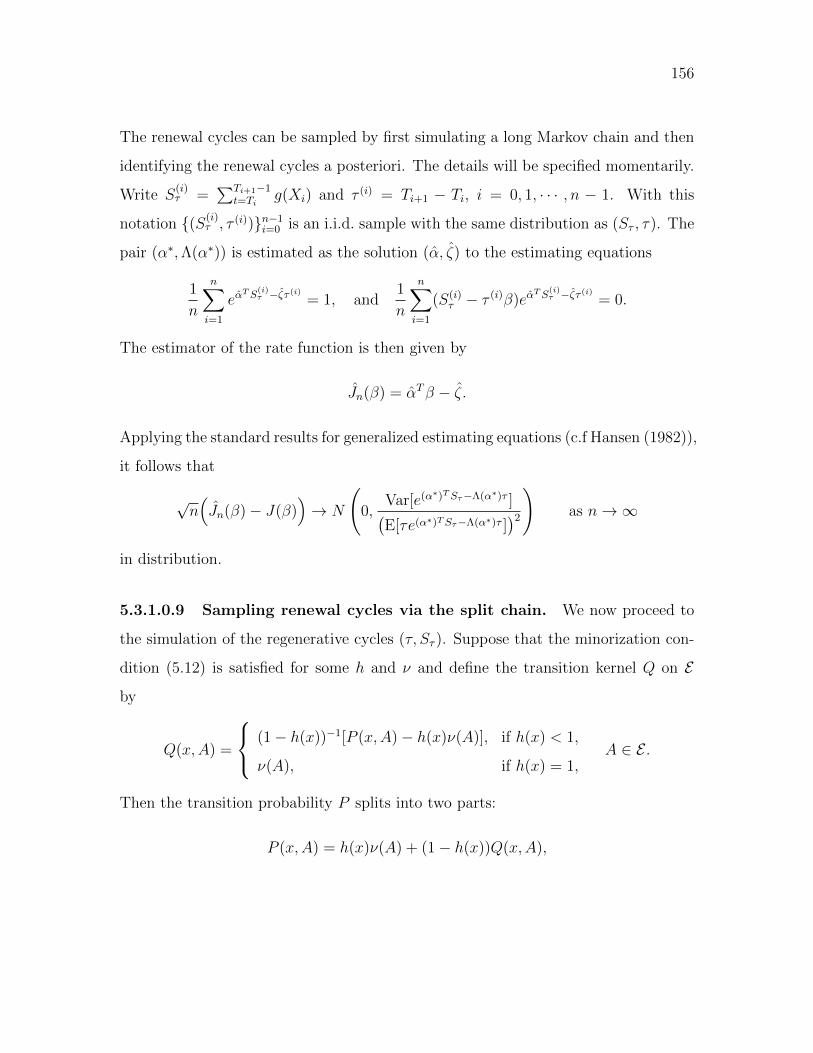
156
The renewal cycles can be sampled by first simulating a long Markov chain and then
identifying the renewal cycles a posteriori. The details will be specified momentarily.
Write S(i)τ =
∑Ti+1−1t=Ti
g(Xi) and τ (i) = Ti+1 − Ti, i = 0, 1, · · · , n − 1. With this
notation (S(i)τ , τ (i))n−1
i=0 is an i.i.d. sample with the same distribution as (Sτ , τ). The
pair (α∗,Λ(α∗)) is estimated as the solution (α, ζ) to the estimating equations
1
n
n∑i=1
eαTS
(i)τ −ζτ (i) = 1, and
1
n
n∑i=1
(S(i)τ − τ (i)β)eα
TS(i)τ −ζτ (i) = 0.
The estimator of the rate function is then given by
Jn(β) = αTβ − ζ .
Applying the standard results for generalized estimating equations (c.f Hansen (1982)),
it follows that
√n(Jn(β)− J(β)
)→ N
(0,
Var[e(α∗)TSτ−Λ(α∗)τ ](E[τe(α∗)TSτ−Λ(α∗)τ ]
)2
)as n→∞
in distribution.
5.3.1.0.9 Sampling renewal cycles via the split chain. We now proceed to
the simulation of the regenerative cycles (τ, Sτ ). Suppose that the minorization con-
dition (5.12) is satisfied for some h and ν and define the transition kernel Q on E
by
Q(x,A) =
(1− h(x))−1[P (x,A)− h(x)ν(A)], if h(x) < 1,
ν(A), if h(x) = 1,A ∈ E .
Then the transition probability P splits into two parts:
P (x,A) = h(x)ν(A) + (1− h(x))Q(x,A),
157
called the Nummelin splitting. Thus, taking one step of the chain from state x can be
interpreted as first throwing a binary coin with probability h(x) for “1” and sample
the next state from ν if the coin comes up “1’ and from Q(x, ·) if it comes up “0”.
Letting Yn;n ≥ 1 denote the incidence process, i.e., the successive results of the
coin tosses, it follows that the times of success, when Yn = 1, are regeneration times.
More precisely, the regeneration times are given by T0 = infn ≥ 1 | Yn = 1 and
Ti = infn > Ti−1 | Yn = 1 for n ≥ 1 (c.f. Section 4.4 of Nummelin (1984)).
In practice, it may be difficult to simulate the chain Xn using Nummelin’s
splitting scheme, because sampling from the transition probability Q is not straight-
forward. Alternatively, the chain can be simulated using an MCMC sampler and the
incidence process Ynn≥1 can subsequently be imputed using its posterior distribu-
tion:
P (Yn+1 = 1 | Xn, Xn+1) = P (Yn+1 = 1 | Xn)dν(·)
dP (Xn, ·)(Xn+1) = h(Xn)
dν(·)dP (Xn, ·)
(Xn+1).
We now consider the above probability in the context of the Metropolis-Hastings
algorithm with proposal q and acceptance probability a. With ν ′ denoting the density
of ν with respect to Lebesgue measure, the posterior probability of success can be
written as
PYn = 1 | Xn, Xn+1 = h(Xn)ν ′(Xn+1)
q(Xn, Xn+1)a(Xn, Xn+1)1Xn 6= Xn+1.
From the imputed values of Y0, Y1, . . . , the regeneration times T0, T1, . . . can be re-
covered, and the independent renewal cycles, XTi , · · · , XTi+1−1, i = 0, . . . , n − 1,
are identified.
158
5.3.2 Computing the Rate Function by the Discretization
Method
In this section an alternative method to compute rate function will be presented. It is
based on solving an eigenvalue problem. Under the same conditions that the pinned
large deviations property holds (Proposition 51), there exits a function r(x;α) such
that the following eigenvalue equation is satisfied (Ney and Nummelin (1987a))∫Eeα
T g(y)r(y;α)P (x, dy) = eΛ(α)r(x;α). (5.15)
When X is an irreducible Markov chain with finite state space, eαT g(y)P (x, dy) is
an irreducible nonnegative matrix, eΛ(α) is the maximal eigenvalue, and r(x;α) is
the corresponding right eigenvector. In this case the computation of the rate function
only involves solving an eigenvalue equation. The computation of the eigenvalues and
eigenvectors can be implemented by standard numerical routines for matrix algebra.
When state space E is infinite, for instance E = Rd, r(x;α) is an eigenfunction
and solving this eigenvalue problem is not straightforward. Numerically, one can
discretize the equation (5.15) and reduce it to an eigenvalue problem for a matrix.
Specifically, taking E = Rd and g(y) = y for example, the equation (5.15) may be
discretized in two steps. First choosing a compact set C = ×di=1[M(i)1 ,M
(i)2 ] ⊂ Rd to
be the discretization range. The set C must be taken such that the integral over E,
on the left hand side of (5.15), is approximated by an integral over C with the same
integrand. The second step is to partition C into mutually exclusive bins of equal size
×di=1(M(i)2 −M
(i)1 )/n(i), resulting in
∏di=1 n
(i) bins, and approximating P (x, dy) and
r(x;α) by their value at a center point inside each bin. For any x, y ∈ C, let Bx and
By denote the bins which x and y lie in and x∗ and y∗ denote their centers. We use
C∗ to denote the collection of centers of the bins. With P ∗(x∗, y∗) =∫By∗
P (x∗, dy),
159
it follows that ∑y∗∈C∗
eαT y∗r(y∗;α)P ∗(x∗, y∗) ≈ eΛ(α)r(x∗;α).
It remains to find the largest eigenvalue for the matrix(eα
T y∗P ∗(x∗, y∗))x∗,y∗∈C∗
and
use it as an approximation for eΛ(α). The approximation error in the second step can
always be reduced by increasing minn(i); 1 ≤ i ≤ d, while the approximation error
in the first step can be controlled when the following limit holds:
supx
∫Cceα
T yr(y;α)P (x, dy)→ 0,
as minminM (i)2 ,−M (i)
1 ; 1 ≤ i ≤ d → ∞.
The discretization method will be used as a comparison to the simulation method
in order to evaluate the precision of the simulation method. The discretization
range and bin size is selected in a trial-and-error manner. When both simulation
method and discretization yield close values, we treat the one by discretization as
the true value. Generally speaking, the discretization method suffers “the curse of
dimensionality” in the sense that the matrix(eα
T y∗P ∗(x∗, y∗))x∗,y∗∈C∗
is of dimen-
sion(∏d
i=1 n(i))×(∏d
i=1 n(i))
, which is formidably high even for moderately large
d. Hence, the use of discretization method is limited for high dimensions. In general
any form of discretization procedure must be used with caution for continuous space
Markov chains, see e.g. Robert and Richardson (1998).
5.4 Numerical Results
In this section the proposed method is demonstrated in a number of examples in-
volving the Metropolis-Hastings algorithm. First, Gaussian target distributions are
considered in combination with Gaussian proposal distributions with scale parameter
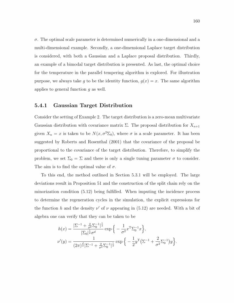
160
σ. The optimal scale parameter is determined numerically in a one-dimensional and a
multi-dimensional example. Secondly, a one-dimensional Laplace target distribution
is considered, with both a Gaussian and a Laplace proposal distribution. Thirdly,
an example of a bimodal target distribution is presented. As last, the optimal choice
for the temperature in the parallel tempering algorithm is explored. For illustration
purpose, we always take g to be the identity function, g(x) = x. The same algorithm
applies to general function g as well.
5.4.1 Gaussian Target Distribution
Consider the setting of Example 2. The target distribution is a zero-mean multivariate
Gaussian distribution with covariance matrix Σ. The proposal distribution for Xn+1
given Xn = x is taken to be N(x, σ2Σ0), where σ is a scale parameter. It has been
suggested by Roberts and Rosenthal (2001) that the covariance of the proposal be
proportional to the covariance of the target distribution. Therefore, to simplify the
problem, we set Σ0 = Σ and there is only a single tuning parameter σ to consider.
The aim is to find the optimal value of σ.
To this end, the method outlined in Section 5.3.1 will be employed. The large
deviations result in Proposition 51 and the construction of the split chain rely on the
minorization condition (5.12) being fulfilled. When imputing the incidence process
to determine the regeneration cycles in the simulation, the explicit expressions for
the function h and the density ν ′ of ν appearing in (5.12) are needed. With a bit of
algebra one can verify that they can be taken to be
h(x) =|Σ−1 + 2
σ2 Σ−10 |
12
|Σ0|12σd
exp− 1
σ2xTΣ−1
0 x,
ν ′(y) =1
(2π)d2 |Σ−1 + 2
σ2 Σ−10 |
12
exp− 1
2yT(Σ−1 +
2
σ2Σ−1
0
)y.
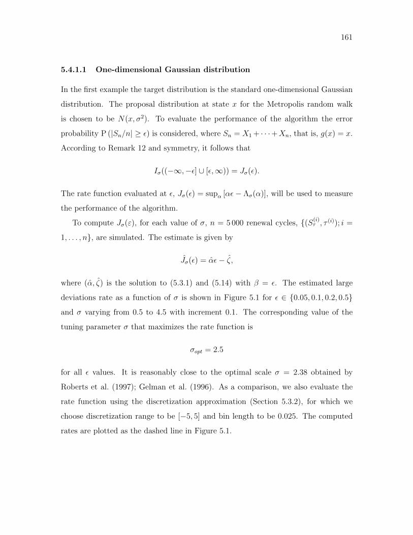
161
5.4.1.1 One-dimensional Gaussian distribution
In the first example the target distribution is the standard one-dimensional Gaussian
distribution. The proposal distribution at state x for the Metropolis random walk
is chosen to be N(x, σ2). To evaluate the performance of the algorithm the error
probability P (|Sn/n| ≥ ε) is considered, where Sn = X1 + · · ·+Xn, that is, g(x) = x.
According to Remark 12 and symmetry, it follows that
Iσ((−∞,−ε] ∪ [ε,∞)) = Jσ(ε).
The rate function evaluated at ε, Jσ(ε) = supα [αε− Λσ(α)], will be used to measure
the performance of the algorithm.
To compute Jσ(ε), for each value of σ, n = 5 000 renewal cycles, (S(i)τ , τ (i)); i =
1, . . . , n, are simulated. The estimate is given by
Jσ(ε) = αε− ζ ,
where (α, ζ) is the solution to (5.3.1) and (5.14) with β = ε. The estimated large
deviations rate as a function of σ is shown in Figure 5.1 for ε ∈ 0.05, 0.1, 0.2, 0.5
and σ varying from 0.5 to 4.5 with increment 0.1. The corresponding value of the
tuning parameter σ that maximizes the rate function is
σopt = 2.5
for all ε values. It is reasonably close to the optimal scale σ = 2.38 obtained by
Roberts et al. (1997); Gelman et al. (1996). As a comparison, we also evaluate the
rate function using the discretization approximation (Section 5.3.2), for which we
choose discretization range to be [−5, 5] and bin length to be 0.025. The computed
rates are plotted as the dashed line in Figure 5.1.
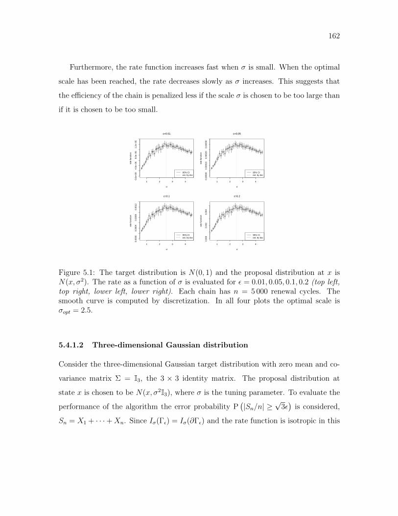
162
Furthermore, the rate function increases fast when σ is small. When the optimal
scale has been reached, the rate decreases slowly as σ increases. This suggests that
the efficiency of the chain is penalized less if the scale σ is chosen to be too large than
if it is chosen to be too small.
1 2 3 4
0.0e
+00
4.0e
−06
8.0e
−06
1.2e
−05
ε=0.01
σ
rate
func
tion
95% CIest. by dsc
1 2 3 4
0.00
000
0.00
010
0.00
020
0.00
030
ε=0.05
σ
rate
func
tion
95% CIest. by dsc
1 2 3 4
0.00
000.
0004
0.00
080.
0012
ε=0.1
σ
rate
func
tion
95% CIest. by dsc
1 2 3 4
0.00
00.
002
0.00
4
ε=0.2
σ
rate
func
tion
95% CIest. by dsc
Figure 5.1: The target distribution is N(0, 1) and the proposal distribution at x isN(x, σ2). The rate as a function of σ is evaluated for ε = 0.01, 0.05, 0.1, 0.2 (top left,top right, lower left, lower right). Each chain has n = 5 000 renewal cycles. Thesmooth curve is computed by discretization. In all four plots the optimal scale isσopt = 2.5.
5.4.1.2 Three-dimensional Gaussian distribution
Consider the three-dimensional Gaussian target distribution with zero mean and co-
variance matrix Σ = I3, the 3 × 3 identity matrix. The proposal distribution at
state x is chosen to be N(x, σ2I3), where σ is the tuning parameter. To evaluate the
performance of the algorithm the error probability P(|Sn/n| ≥
√3ε)
is considered,
Sn = X1 + · · ·+Xn. Since Iσ(Γε) = Iσ(∂Γε) and the rate function is isotropic in this

163
case, it follows that Jσ(β1) = Jσ(β2) whenever |β1| = |β2|. Therefore, it is sufficient
to evaluate Jσ at one location on the sphere x : |x| =√
3ε.
For σ in the range from 0.5 to 2.5 with increment 0.01 and ε ∈ 0.01, 0.05, 0.1, 0.2
the rate Iσ(ε1) is evaluated. The simulation is based on n = 5 000 independent
renewal cycles. The evaluation of the rate as a function of σ is displayed in Figure
5.2. We fit a concave curve to the rate function as a function of σ. The numerically
optimized scale parameter based on the fitted curves is
σopt = 1.4
for all ε = 0.01, 0.05, 0.1, 0.2, which is close to the result 1.37 reported in Roberts
et al. (1997), Gelman et al. (1996). We refrain from using the discretization method
in this example because the computational cost is high.
5.4.2 Laplace Target Distribution
Consider a Laplace target distribution with density function
π(x) = (1/2)e−|x|.
In this section, two proposal distributions for Xn+1 given Xn = x will be studied: the
Laplace proposal and the Gaussian proposal. In both cases, it is straightforward to
check that the minorization condition holds. With a bit of algebra, expressions for h
and ν can be derived. If the proposal is a Laplace distribution with scale parameter
σ,
qL(x, y) = (2σ)−1e−|y−x|/σ,
then h and ν ′ can be taken as
hL(x) =e|x|σ
σ + 1, ν ′L(y) =
σ + 1
2σeσ+1σ|y|.
164
0.5 1.0 1.5 2.0 2.5
0.0e
+00
5.0e
−06
1.0e
−05
1.5e
−05
ε=0.01
σ
rate
func
tion
by cnvx reg
0.5 1.0 1.5 2.0 2.50e
+00
1e−
042e
−04
3e−
044e
−04
ε=0.05
σ
rate
func
tion
by cnvx reg
0.5 1.0 1.5 2.0 2.5
0.00
000.
0005
0.00
100.
0015
ε=0.1
σ
rate
func
tion
by cnvx reg
0.5 1.0 1.5 2.0 2.5
0.00
00.
002
0.00
40.
006
ε=0.2
σ
rate
func
tion
by cnvx reg
Figure 5.2: The target distribution is N3(0, I3) and the proposal distribution atx is N3(x, σ2I3). The rate as a function of σ is evaluated for ε1, where ε =0.01, 0.05, 0.1, 0.2 (top left, top right, lower left, lower right). Each chain has n = 5 000renewal cycles. The solid curve is estimated by convex regression. In all four plotsthe optimal value of σ is σopt = 1.4.

165
If the proposal distribution is N(x, σ2), then
hN(x) =√
2πeσ2
4+ x2
σ2 Φ(σ2
2
), ν ′N(y) =
e−y2
σ2−|y|
√4πσe
σ2
4 Φ(σ2
2),
where Φ denotes the standard normal distribution function. As in Section 5.4.1.1 the
error probability will be taken as P (|Sn/n| ≥ ε). The rate function is evaluated at ε,
Jσ(ε) = supα [αε− Λσ(α)], for ε ∈ 0.01, 0.1 and σ in the range from 1 to 7 with an
increment of 0.1.
The rate as a function of σ for the Laplace proposals, computed based on n =
10 000 renewal cycles, is illustrated in the top row of Figure 5.3. We conclude that
the optimal scaling parameter, for the Laplace proposal, is σopt = 4.0 for both ε =
0.01, 0.1.
The rate function for the Gaussian proposal distribution is computed based on
n = 10 000 renewal cycles and is illustrated in the bottom row in Figure 5.3. In
this case the optimal scale parameter is σopt = 4.5 for both ε = 0.01, 0.1. The rate
functions computed using the discretization method are also show in the figure, for
which we choose the discretization range to be [−10, 10] with bin length equal to 0.05.
An interesting observation is that for the same choice of ε the maximum rate of
the Gaussian proposal is slightly higher than the maximum rate of the Laplacian
proposal. Thus, when the target distribution is a Laplace distribution, the best
Gaussian proposal outperforms the best Laplace proposal.
5.4.3 A Bimodal Target Distribution
In this section we consider an example with a bimodal target distribution and the
proposal distribution is a mixture distribution. More precisely, the target distribution

166
1 2 3 4 5 6 7
0e+
002e
−06
4e−
06ε=0.01
σ
lapl
acia
n pr
opos
al
95% CIest. by dsc
1 2 3 4 5 6 7
0e+
002e
−04
4e−
04
ε=0.1
σ
lapl
acia
n pr
opos
al
95% CIest. by dsc
2 3 4 5 6 7
0e+
002e
−06
4e−
06
ε=0.01
σ
Gau
ssia
n pr
opos
al
95% CIest. by dsc
2 3 4 5 6 7
0e+
002e
−04
4e−
04ε=0.1
σ
Gau
ssia
n pr
opos
al
95% CIest. by dsc
Figure 5.3: The target distribution is standard one-dimensional Laplace distribution.In the upper two plots the proposal distribution at x is Laplacian, centered at x. Therate as a function of σ is evaluated at ε = 0.01, 0.1 (left, right). The computation isbased on n = 10 000 renewal cycles. The smooth curve is estimated by discretization.The optimal scale is σopt = 4.0 for both ε = 0.01, 0.1. In the lower two plots theproposal distribution at x is N(x, σ2). The rate as a function of σ is evaluated atε = 0.01, 0.1 (left, right). The computation is based on n = 10 000 renewal cycles.The smooth curve is estimated by discretization. The optimal scale is σopt = 4.5 forboth ε = 0.01, 0.1.

167
is a mixture of two d-dimensional Gaussian distributions and its density has the form
π(x) =1
2(2π)−d/2|Σ1|−1/2 exp
− 1
2(x− µ1)TΣ−1
1 (x− µ1)
+1
2(2π)−d/2|Σ2|−1/2 exp
− 1
2(x− µ2)TΣ−1
2 (x− µ2). (5.16)
This target distribution is studied in Craiu et al. (2009) in the context of adaptive
MCMC.
The proposal distribution of the Metropolis-Hastings algorithm can be described
as follows. The state space Rd is partitioned into two regions S1 and S2, that is
S1 ∪ S2 = Rd and S1 ∩ S2 = ∅, in such a way that each region contains one mode.
The proposal distribution depends on whether the current state belongs to S1 or S2.
For x ∈ S1 the proposal distribution is a mixture of the form
q1(x, y) = p(2π)−d/2σ−d|Σ1|−1/2 exp− (y − x)TΣ−1
1 (y − x)
2σ2
+ (1− p)(2π)−d/2σ−2|Σ2|−1/2 exp
− (y − x)TΣ−1
2 (y − x)
2σ2
,
whereas for x ∈ S2 the proposal distribution has the form
q2(x, y) = (1− p)(2π)−d/2σ−d|Σ1|−1/2 exp− (y − x)TΣ−1
1 (y − x)
2σ2
+ p(2π)−d/2σ−2|Σ2|−1/2 exp
− (y − x)TΣ−1
2 (y − x)
2σ2
,
where p ∈ (0, 1) is the tuning parameter to be optimized. Here the scale parameter
is taken to be σ = 2.38/√d where d is the dimension. The basic idea is to apply the
optimal proposal corresponding to Σ1 in region S1 and to apply that to Σ2 in region
S2.
Let us consider the two-dimensional case. The parameters are taken to be
µ1 = (3, 0)T, Σ1 = I2, µ2 = (−3, 0)T, Σ2 = 3I2.
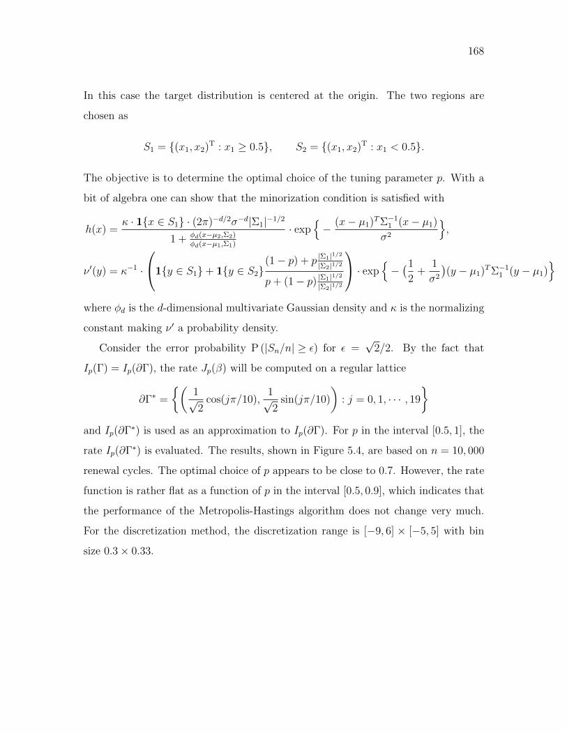
168
In this case the target distribution is centered at the origin. The two regions are
chosen as
S1 = (x1, x2)T : x1 ≥ 0.5, S2 = (x1, x2)T : x1 < 0.5.
The objective is to determine the optimal choice of the tuning parameter p. With a
bit of algebra one can show that the minorization condition is satisfied with
h(x) =κ · 1x ∈ S1 · (2π)−d/2σ−d|Σ1|−1/2
1 + φd(x−µ2,Σ2)φd(x−µ1,Σ1)
· exp− (x− µ1)TΣ−1
1 (x− µ1)
σ2
,
ν ′(y) = κ−1 ·
1y ∈ S1+ 1y ∈ S2(1− p) + p |Σ1|1/2
|Σ2|1/2
p+ (1− p) |Σ1|1/2|Σ2|1/2
· exp−(1
2+
1
σ2
)(y − µ1)TΣ−1
1 (y − µ1)
where φd is the d-dimensional multivariate Gaussian density and κ is the normalizing
constant making ν ′ a probability density.
Consider the error probability P (|Sn/n| ≥ ε) for ε =√
2/2. By the fact that
Ip(Γ) = Ip(∂Γ), the rate Jp(β) will be computed on a regular lattice
∂Γ∗ =
(1√2
cos(jπ/10),1√2
sin(jπ/10)
): j = 0, 1, · · · , 19
and Ip(∂Γ∗) is used as an approximation to Ip(∂Γ). For p in the interval [0.5, 1], the
rate Ip(∂Γ∗) is evaluated. The results, shown in Figure 5.4, are based on n = 10, 000
renewal cycles. The optimal choice of p appears to be close to 0.7. However, the rate
function is rather flat as a function of p in the interval [0.5, 0.9], which indicates that
the performance of the Metropolis-Hastings algorithm does not change very much.
For the discretization method, the discretization range is [−9, 6] × [−5, 5] with bin
size 0.3× 0.33.
169
0.5 0.6 0.7 0.8 0.9 1.0
0e+
001e
−04
2e−
043e
−04
4e−
045e
−04
6e−
04
p
rate
func
tion
Figure 5.4: The target distribution is a bi-modal mixture of two 2-dimensionalGaussian distributions and the proposal density is given by q1 and q2. The rate asa function of the mixing parameter p is evaluated on circle |x| = ε = 1√
2. The
computation is based on n = 10 000 renewal cycles. The smooth curve is estimatedby discretization. The optimal value of the mixing parameter is popt = 0.7.
170
5.4.4 Tuning the temperature for parallel tempering
Parallel tempering is usually employed to improve the convergence of MCMC algo-
rithms. The essence of a parallel tempering algorithm can be formulated as follows.
Let π denote the density function of the target distribution, and a series of tem-
peratures 1 = T (1) < T (2) < · · · < T (k) is selected. At temperature T (i), a chain
X(i)n ;n ≥ 0 is generated with target density proportional to π
1
T (i) and transitional
probability P (i)(x, dy). In addition, at some time a swap between samples from a pair
of chains is carried out with probability
min
1,[π(x(j))
π(x(i))
] 1
T (i)− 1
T (j)
, (5.17)
where the two states x(i) and x(j) are from the ith and the jth chain, respectively.
This swap allows the chains in low temperature to access the states that are less
likely to be explored in their own right. In practice, the swap is often within chains
of adjacent temperatures.
A problem of interest is the selection of temperature levels. Ideally, one can choose
as many temperatures as computation resources allow. However, it could be a waste
if T (i) and T (i+1) are too close, since these two chains will have very similar dynamic
properties and there is little gain in including both. However, as T (i+1)−T (i) increases,
the acceptance probability (5.17) decreases.
We apply our efficiency measure to the choice of temperature levels. As an illus-
tration, we present a relatively simple scenario that contains two temperature levels
1 = T (1) < T (2). Our task is to find the optimal T (2). Assume
π(x) =1
2√
2π
[exp
− (x− µ)2
2
+ exp
− (x+ µ)2
2
],
x ∈ R, which is a mixture of two normals. Two parallel chains X(i)n ;n ≥ 0, i = 1, 2
are simulated, and each admits stationary distribution with density proportional to
171
π1
T (i) . The initial states (X(1)0 = x
(1)0 , X
(2)0 = x
(2)0 ) are randomized. At any time
n ≥ 1, under T (i), i = 1, 2, the ith chain is first updated according to the Metropolis-
Hastings algorithm with a Gaussian proposal N(X
(i)n−1, (σ
(i))2)
and the updated state
is denoted by y(i)n . Then a swap between y
(1)n and y
(2)n is carried out with probability
(5.17), that is, X(1)n = y
(2)n and X
(2)n = y
(1)n .
Let π04= supπ(x);x ∈ R. Then the transition probability of the above algorithm
satisfies the minorization condition (5.12) with:
h(x1, x2) =c
2πσ(1)σ(2)exp
− x2
1
(σ(1))2 −
x22
(σ(2))2
ν ′(y1, y2) =
1
cexp
− y2
1
(σ(1))2 −
y22
(σ(2))2
· π(y1)π
1
T (2) (y2)
π1+ 1
T (2)
0
×(
1−min
1,[π(y2)
π(y1)
]1− 1
T (2)
)+
1
cexp
− y2
2
(σ(1))2 −
y21
(σ(2))2
× π(y2)π
1
T (2) (y1)
π1+ 1
T (2)
0
·min
1,[π(y1)
π(y2)
]1− 1
T (2)
and c is a normalizing constant that makes ν ′ a valid probability density function on
R2.
In our simulation, parameters are set as µ = 3, σ(1) = 1, σ(2) = 2. The parallel
tempering algorithm is executed for a series of temperature levels T (2), where 1/T (2)
takes values on the lattice 0.02, 0.04, · · · , 1, with increment 0.02. For each chain, the
error probability P(|S(1)n /n| ≥ 0.5
)is considered and the rate function is calculated
with 10 000 renewal cycles. The rate function as a function of the inverse temperature
1/T (2) is displayed in Figure 5.5. The optimal choice for T (2) under this setting is
T(2)opt = 1/0.22 = 4.55. It is observed that the algorithms is improved when T (2)
increases from 1 to 4.55. If the temperature further increases, the performance will
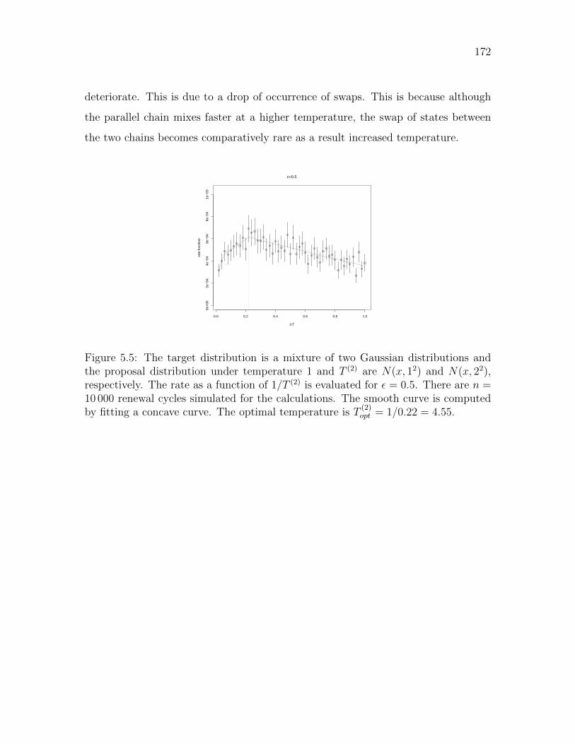
172
deteriorate. This is due to a drop of occurrence of swaps. This is because although
the parallel chain mixes faster at a higher temperature, the swap of states between
the two chains becomes comparatively rare as a result increased temperature.
0.0 0.2 0.4 0.6 0.8 1.0
0e+
002e
−04
4e−
046e
−04
8e−
041e
−03
ε=0.5
1/T
rate
func
tion
Figure 5.5: The target distribution is a mixture of two Gaussian distributions andthe proposal distribution under temperature 1 and T (2) are N(x, 12) and N(x, 22),respectively. The rate as a function of 1/T (2) is evaluated for ε = 0.5. There are n =10 000 renewal cycles simulated for the calculations. The smooth curve is computedby fitting a concave curve. The optimal temperature is T
(2)opt = 1/0.22 = 4.55.

173
Bibliography
Adler, R., Blanchet, J., and Liu, J. (2012), “Efficient Monte Carlo for Large Excur-sions of Gaussian Random Fields,” Ann. Appl. Probab., 22, 1167–1214. 108
Asmussen, S., Binswanger, K., and Hojgaard, B. (2000), “Rare events simulation forheavy-tailed distributions,” Bernoulli, 6, 303–322. 103
Asmussen, S. and Glynn, P. (2007), Stochastic Simulation: Algorithms and Analysis,New York, NY, USA: Springer. 103
Asmussen, S. and Kroese, D. (2006), “Improved algorithms for rare event simulationwith heavy tails,” Adv. Appl. Probab., 38, 545–558. 103
Babu, G. J. (1986), “A note on bootstrapping the variance of sample quantile,” Ann.I. Stat. Math., 38, 439–443. 103
Baddeley, A. (2006), “Spatial Point Processes and their Applications,” in StochasticGeometry: Lectures given at the C.I.M.E. Summer School held in Martina Franca,Italy, September 13–18, 2004, eds. Baddeley, A., Barany, I., Schneider, R., andWeil, W., Springer Verlag, Lecture Notes in Mathematics 1892, pp. 1–75. 15, 50
Bahadur, R. R. (1966), “A Note on Quantiles in Large Samples,” Ann. Math. Stat.,37. 102, 103
Bai, Y., Song, P. X.-K., and Raghunathan, T. E. (2012), “Joint composite estimatingfunctions in spatiotemporal models,” J. Roy. Stat. Soc. B, 74, 799–824. 54
Baxendale, P. H. (2005), “Renewal Theory and Computable Convergence Rates forGeometrically Ergodic Markov Chains,” Ann. Appl. Probab., 700–738. 142, 145
Besag, J. and Green, P. J. (1993), “Spatial Statistics and Bayesian Computation,” J.R. Stat. Soc. Ser. B Stat. Methodol., 55, 25–37. 142
174
Bevilacqua, M., Gaetan, C., Mateu, J., and Porcu, E. (2012), “Estimating Space andSpace-Time Covariance Functions for Large Data Sets: A Weighted CompositeLikelihood Approach,” J. Am. Stat. Assoc., 107, 268–280. 54, 59
Blachet, J. (2009), “Efficient importance sampling for binary contingency tables,”Ann. Appl. Probab., 19, 949–982. 108
Blanchet, J. and Glynn, P. (2008), “Effcient rare event simulation for the maximumof heavy-tailed random walks,” Ann. Appl. Probab. 103
Blanchet, J., Glynn, P., and Liu, J. (2007a), “Efficient Rare-Event Simulation forHeavy-tailed Multiserver Queues. Preprint,” . 103
— (2007b), “Fluid heuristics, Lyapunov bounds and efficient importance samplingfor a heavy-tailed G/G/1 queue,” Queueing Syst., 57, 99–113. 108
Blanchet, J. and Liu, J. (2008), “State-Dependent Importance Sampling for RegularlyVarying Random Walks,” Adv. Appl. Probab., 40, 1104–1128. 103, 108
— (2010), “Efficient Importance Sampling in Ruin Problems for MultidimensionalRegularly Varying Random Walks,” J. Appl. Probab., 47, 301–322. 103
Bolthausen, E. (1982), “On the Central Limit Theorem for Stationary Mixing Ran-dom Fields,” Ann. Probab., 10, 1047–1050. 8, 12, 16, 28
Bradley, R. C. (2005), “Basic Properties of Strong Mixing Conditions. A Survey andSome Open Questions,” Probab. Surv., 2, 107–144. 1, 8, 55
Bucklew, J. (2004), Introduction to Rare Event Simulation, New York, NY, USA:Springer. 103
Bulinski, A. V. and Shashkin, A. P. (2007), Limit Theorems for Associated RandomFields and Related Systems, World Scientific. 1, 9, 16, 42, 47
Chu, F. and Nakayama, M. K. (2010), “Confidence intervals for quantiles and value-at-risk when applying importance sampling,” in Proceedings of the 2010 WinterSimulation Conference. 103, 108
Craiu, R. V., Rosenthal, J., and Yang, C. (2009), “Learn From Thy Neighbor:Parallel-Chain and Regional Adaptive MCMC,” J. Amer. Statist. Assoc., 104,1454–1466. 143, 167
175
Damian, D., Sampson, P. D., and Guttorp, P. (2003), “Variance modeling for nonsta-tionary spatial processes with temporal replications,” J. Geophys. Res., 108, 8778.53
David, H. A. and Nagaraja, H. N. (2003), Order Statistics, New Jersey: Wiley-Interscience, 3rd ed. 103
Davis, A. R. and Yau, C. Y. (2011), “Comments on Pairwise Likelihood in TimeSeries Models,” Stat. Sinica, 21, 255–277. 54
Davis, R. A., Kluppelberg, C., and Steinkohl, C. (2013), “Statistical Inference forMax-Stable Processes in Space and Time,” J. Roy. Stat. Soc. B, 75, 791–819. 54
Davis, R. A., Liu, J., and Yang, X. (2014), “On Central Limit Theorems For RandomFields and Weak Dependence,” Preprint. 71, 86, 87
Davis, R. A. and Rodriguez-Yam, G. (2005), “Estimation for state-space models basedon a likelihood approximation,” Statistica Sinica, 15, 381–406. 64
de Haan, L. and Ferreira, A. (2006), Extreme Value Theory: An Introduction,Springer. 21
de la Pena, V. H., Lai, T. L., and Shao, Q. (2009), Self-Normalized Processes, BerlinHeidelberg: Springer-Verlag. 136
Dedecker, J., Doukhan, P., Lang, G., Leon R., J. R., Louhichi, S., and Prieur, C.(2007), Weak Dependence: With Examples and Applications, Springer. 2, 7, 10, 12,18, 42, 43, 55, 70
Dembo, A. and Zeitouni, O. (1998), Large Devations Techniques and Applicaitons,New York, NY: Springer, 2nd ed. 150
Doukhan, P. (1995), Mixing: Properties and Examples, Springer-Verlag. 1, 8, 42, 44,55
Doukhan, P. and Louhichi, S. (1999), “A new weak dependence condition and appli-cations to moment inequalities,” Stoch. Proc. Appl., 84, 313–342. 1, 7, 10, 19
Dupuis, P. and a H. Wang, A. S. (2007), “Dynamic importance sampling for queueingnetworks,” Ann. Appl. Probab., 17, 1306–1346. 103
Dupuis, P. and Ellis, R. S. (1997), A Weak Convergence Approach to the Theory ofLarge Deviations, New York, NY: Wiley & Sons, Inc., 1st ed. 150
176
Dupuis, P., Leder, K., and Wang, H. (2007), “Importance sampling for sums of ran-dom variables with regularly varying tails,” ACM Trans. Model. Comput. Simul.,17, 14. 103
Dupuis, P. and Wang, H. (2005), “Dynamic Importance Sampling for UniformlyRecurrent Markov Chains,” Ann. Appl. Probab., 15, 1–38. 103, 108
Durrett, R. (2010), Probability: Theory and Examples, Cambridge University Press.29, 117
Falk, M. (1986), “On the estimation of the quantile density function,” Stat. Probab.Lett., 4, 69–73. 103
Gaetan, C. and Guyon, X. (2010), Spatial Statistics and Modeling, Springer. 1, 58,61
Gelman, A., Carlin, J. B., Stern, H. S., and Rubin, D. B. (2010), Bayesian DataAnalysis, Boca Raton: Chapman & Hall/CRC, 2nd ed. 142
Gelman, A., Roberts, G., and Gilks, W. (1996), “Efficient Metropolis Jumping Rules,”in Bayesian Statistics, eds. Bernado, J. M. et al., Oxford University Press, vol. 5,pp. 599–607. 142, 161, 163
Gelman, A. and Rubin, D. B. (1992), “Inference from Iterative Simulation UsingMultiple Sequences,” Stat. Sci., 7, 457–472. 143
Ghosh, M., Parr, W. C., Singh, K., and Babu, G. J. (1985), “A note on bootstrappingthe sample median,” Ann. Stat., 12, 1130–1135. 103
Gilks, W. R., Richardsson, S., and Spiegelhalter, D. J. (1996), Markov Chain MonteCarlo in Practice, Chapman & Hall. 142
Glasserman, P., Heidelberger, P., and Shahabuddin, P. (1999), “Importance samplingand stratification for Value-at-Risk,” in Computational Finance 1999 (Proc. of theSixth Internat. Conf. Comput. Finance), Cambridge, MA: MIT Press, pp. 7–24.102
— (2000), “Variance reduction techniques for estimating value-at-risk,” Manage. Sci.,46, 1349–1364. 102
— (2002), “Portfolio value-at-risk with heavy-tailed risk factors,” Math. Financ., 12,239–270. 103
177
Glasserman, P. and Li, J. (2005), “Importance sampling for the portfolio credit risk,”Manage. Sci., 50, 1643–1656. 102
Glynn, P. W. (1996), “Importance sampling for Monte Carlo estimation of quantiles,”Mathematical Methods in Stochastic Simulation and Experimental Design: Proc.2nd St. Petersburg Workshop on Simulation, 180–185. 3, 103, 107
Guyon, X. (1995), Random Field on a Network: Modeling, Statistics and Applications,Springer-Verlag. 12
Haario, H., Saksman, E., and Tamminen, J. (2001), “An Adaptive Metropolis Algo-rithm,” Bernoulli, 7, 223–242. 143
Hall, P. and Martin, M. A. (1988), “Exact convergence rate of bootstrap quantilevariance estimator,” Probab. Theory Rel., 80, 261–268. 4, 103, 107, 110
Hansen, L. P. (1982), “Large Sample Properties of Generalized Method of MomentsEstimators,” Econometrica, 50, 1029–1054. 156
Hastings, W. K. (1970), “Monte Carlo sampling methods using Markov chains andtheir applications,” Biometrika, 57, 97–109. 146
Huang, W., Wang, K., Breidt, F. J., and Davis, R. A. (2011), “A Class of StochasticVolatility Models for Environmental Applications,” J. Time. Ser. Anal, 32, 364–377. 2, 53, 56, 64
Hult, H. and Svensson, J. (2009), “Efficient calculation of risk measures by importancesampling - the heavy tailed case,” Preprint. 102, 103, 107, 108
Jenish, N. and Prucha, I. (2009), “Central Limit Theorems and Uniform Laws ofLarge Numbers for Arrays of Random Fields,” J. Econometrics, 150, 86–98. 8, 12
— (2012), “On Spatial Processes and Asymptotic Inference under Near-Epoch De-pendence,” J. Econometrics, 170, 178–190. 8, 12
Juneja, S. and Shahabuddin, P. (2002), “Simulating heavy tailed processes usingdelayed hazard rate twisting,” ACM Trans. Model. Comput. Simul., 12, 94–118.103
Karr, A. F. (1986), “Inferrence for Stationary Random Fields Given Poisson Sam-ples,” Adv. Appl. Probab., 18, 406–422. 54
178
Komlos, J., Major, P., and Tusnady, G. (1975a), “An approximation of partial sums ofindependent RV’-s and the sample DF. I,” Wahrsch verw Gebiete/Probab. TheoryRel., 32, 111–131. 104, 120, 128
— (1975b), “Weak convergence and embedding,” Limit Theorems of Probability The-ory. Colloquia Mathematica Societatis Janos Bolyai, 11, 149–165. 120, 128
— (1976), “An approximation of partial sums of independent r.v.’s and the sampledf. II,” Wahrsch verw Gebiete/Probab. Theory Rel., 34, 33–58. 121, 128
Kontoyiannis, I., Lastras-Montano, L. A., and Meyn, S. P. (2005), “Relative entropyand exponential deviation bounds for general Markov chains,” in Information Theo-ry, 2005. ISIT 2005. Proceedings. International Symposium on Information Theory,pp. 1563–1567. 150
— (2006), “Exponential bounds and stopping rules for MCMC and general Markovchains,” in Proceedings of the 1st International Conference on Performance Evalu-ation Methodolgies and Tools, New York, NY, USA: ACM, valuetools ’06. 150
Lahiri, S. N. (2003), “Central limit theorems for weighted sums of a spatial processunder a class of stochastic and fixed designs.” Sankhya A, 65, 356–388. 8
Li, B., Genton, M. G., and Sherman, M. (2008), “On the Asymptotic Joint Dis-tribution of Sample Space-Time Covariance Estimators,” Bernoulli, 14, 228–248.54
Liu, J. and Yang, X. (2012), “The convergence rate and asymptotic distribution ofthe bootstrap quantile variance estimator for importance sampling,” Adv. Appl.Probab., 44, 815–841. 3, 101
Maritz, J. S. and Jarrett, R. G. (1978), “A note on estimating the variance of thesample median,” J. Am. Stat. Assoc., 73, 194–196. 103
McKean, J. W. and Schrader, R. M. (1984), “A comparison of methods for studen-tizing the sample median,” Commun. Stat.-Simul. C., 13, 751–773. 103
Mengersen, K. L. and Tweedie, R. L. (1996), “Rates of Convergence of the Hastingsand Metropolis Algorithms,” Ann. Stat., 24, 101–121. 142, 150
Metropolis, N., Rosenbluth, A. W., Rosenbluth, M. N., Teller, A. H., and Teller, E.(1953), “Equations of State Calculations by Fast Computing Machines,” J. Chem.Phys., 21, 1087C1092. 146
179
Meyn, S. P. and Tweedie, R. L. (2009), Markov Chains and Stochastic Stability, NewYork: Cambridge University Press, 2nd ed. 142, 145
Møller, J. (2003), “Shot Noise Cox Processes,” Advances in Applied Probability, 35,614–640. 22
Møller, J. and Waagepetersen, R. P. (2003), Statistical inference and simulation forspatial point processes, Chapman and Hall/CRC. 59
Ney, P. and Nummelin, E. (1987a), “Markov Additive Processes I. Eigenvalue Prop-erties and Limit Theorems,” Ann. Probab., 15, 561–592. 4, 144, 150, 152, 155,158
— (1987b), “Markov Additive Processes II. Large Deviations,” Ann. Probab., 15,593–609. 4, 144, 150
Ng, C. T., Joe, H., Karlis, D., and Liu, J. (2011), “Composite Likelihood for TimeSeries Models with a Latent Autoregressive Process,” Stat. Sinica, 21, 279–305. 54
Nordman, D. J. and Lahiri, S. N. (2004), “On optimal spatial subsample size forvariance estimation,” Ann. Stat., 32, 1981–2027. 66
Nummelin, E. (1984), General Irreducible Markov Chains and Non-negative Opera-tors, Cambridge: Cambridge University Press. 157
Palacios, M. B. and Steel, M. F. J. (2006), “Non-Gaussian Bayesian GeostatisticalModeling,” J. Am. Stat. Assoc., 101, 604–618. 2, 53, 56
Politis, D. N., Romano, J. P., and Wolf, M. (2001), “On the Asymptotic Thoery ofSubsampling,” Stat. Sinica, 11, 1105–1124. 66
Resnick, S. I. (2007), Heavy-tailed Phenomena: Probabilistic and Statistical Modeling,Springer. 21
Robert, C. P. and Richardson, S. (1998), “Markov Chain Monte Carlo Method,” inDiscretization and MCMC Convergence Assessment, ed. Robert, C. P., New York,NY: Springer-Verlag. 143, 159
Roberts, G. O., Gelman, A., and Gilks, W. R. (1997), “Weak Convergence and Op-timal Scaling of Random Walk Metropolis Algorithms,” Ann. Appl. Probab., 7,110–120. 143, 161, 163
180
Roberts, G. O. and Rosenthal, J. S. (1998), “Optimal Scaling of Discrete Approxima-tions to Langevin Diffusions,” J. R. Stat. Soc. Ser. B Stat. Methodol., 60, 255–268.143
— (2001), “Optimal Scaling for Various Metropolis-Hastings Algorithms,” Stat. Sci.,16, 351–367. 160
— (2007), “Coupling and ergodicity of adaptive Markov chain Monte Carlo algo-rithms,” J. Appl. Probab., 44, 458–475. 143
— (2009), “Examples of adaptive MCMC,” J. Comput. Graph. Stat., 18, 349–367.143
Roberts, G. O. and Tweedie, R. L. (1999), “Bounds on regeneration times and con-vergence rates for Markov chains,” Stoch. Proc. Appl., 80, 211–229. 142
Rosenthal, J. S. (1995), “Minorization Conditions and Convergence Rates for MarkovChain Monte Carlo,” J. Amer. Statist. Assoc., 90, 558–566. 142, 145
— (2011), “Optimal Proposal Distributions and Adaptive MCMC,” in Handbook ofMarkov Chain Monte Carlo, eds. Brooks, S., Gelman, A., Jones, G. L., and Meng,X.-L., Chapman & Hall/CRC. 143
Sadowsky, J. (1996), “On Monte Carlo estimation of large deviations probabilities,”Ann. Appl. Probab., 6, 399–422. 103
Shashkin, A. P. (2002), “Quasi-associatedness of a Gaussian system of random vec-tors,” Russ. Math. Surv., 57, 1243–1244. 19
Sheather, S. J. (1986), “A finite sample estimate of the variance of the sample medi-an,” Stat. Probab. Lett., 4, 1815–1842. 103
Sherman, M. (2010), Spatial statistics and spatio-temporal data : covariance functionsand directional properties, Wiley. 65, 66
Siegmund, D. (1976), “Importance sampling in the Monte Carlo study of sequentialtests,” Ann. Stat., 4, 673–684. 103
Steel, M. and Fuentes, M. (2010), “Non-Gaussian and Nonparametric Models forCountinuous Spatial Data,” in Handbook of Spatial Statistics, eds. Gelfand, A.,Diggle, P., Fuentes, M., and Guttorp, P., Chapman & Hall/CRC, pp. 149–167. 2,53

181
Stein, M. L. (1999), Interpolation of spatial data: some theory for kriging, Springer.19
Stoer, J. and Bulirsch, R. (1993), Introduction to numerical analysis, Springer-Verlag,2nd ed. 65, 99
Sun, L. and Hong, L. J. (2009), “A general framework of importance sampling forvalue-at-risk and conditional value-at-risk,” in Proceedings of 2009 Winter Simula-tion Conference, pp. 415–422. 102
— (2010), “Asymptotic representations for importance-sampling estimators of value-at-risk and conditional value-at-risk,” Oper. Res. Lett., 38, 246–251. 102
Varin, C., Reid, N., and Firth, D. (2011), “An overview of composite likelihoodmethods,” Stat. Sinica, 21, 5–42. 59
Wang, R.-H., Lin, S.-K., and Fuh, C.-D. (2009), “An importance sampling methodto evaluate value-at-risk for asset with jump risk,” Asia-Pac. J. Financ. St., 38,745–772. 102


![[BOOK] [Bootstrap] [Awesome] Bootstrap-Programming-Cookbook](https://img.pdfslide.us/doc/110x75/577ca6bf1a28abea748c023f/book-bootstrap-awesome-bootstrap-programming-cookbook.jpg)