1

Linear and Quadratic Approximations Back in Topic 4.6 (from Calculus AB), we learned that if a function is differentiable at a point c then it can be approximated

near c by its tangent line, which we called the linear approximation to f at the point c. Furthermore, we rewrote the point-slope

version of that line, 𝑦 − 𝑓(𝑐) = 𝑓 ′(𝑐)(𝑥 − 𝑐) as

𝐿(𝑥) = 𝑓(𝑐) + 𝑓 ′(𝑐)(𝑥 − 𝑐).

Because this linear approximation is a first-degree polynomial of x, we can name it 𝑃1(𝑥):

𝑃1(𝑥) = 𝑓(𝑐) + 𝑓 ′(𝑐)(𝑥 − 𝑐).

This polynomial has some important properties.

1.) It matches the function f in value at x = c. P1(c) = f (c) + ¢f (c)(c- c) = f (c)

2.) It matches the slope of the function f in value at x = c. P1¢(c) = 0 + ¢f (c)(1) = ¢f (c)

The problem is that linear approximations don’t always work so well when the graph of f has a great deal of “curvature” near c.

To fix this problem, we can create a quadratic approximating polynomial by adding one new term to the linear polynomial. We

can denote the new polynomial 𝑃2(𝑥) and it would look like

𝑃2(𝑥) = 𝑓(𝑐) + 𝑓 ′(𝑐)(𝑥 − 𝑐) + 𝑎(𝑥 − 𝑐)2

Notice that we will need to find the value of the coefficient a. To determine a and to

ensure that 𝑃2(𝑥) is a good approximation for f near the point c we require that 𝑃2(𝑥)

agree with f in value, slope and concavity at c. In other words, 𝑃2(𝑥) must satisfy the

conditions:

P2(c) = f (c) + ¢f (c)(c - c) + a(c- c)2 = f (c)

P2¢(x) = 0 + ¢f (c)(1) + 2a(x - c) ® P

2¢(c) = ¢f (c) + 2a(c - c) = ¢f (c)

P2¢¢(x) = 2a ® P

2¢¢(c) = 2a must be equivalent to ¢¢f (c) ® a =

1

2¢¢f (c)

Therefore, the resulting quadratic approximating polynomial is

𝑃2(𝑥) = 𝑓(𝑐) + 𝑓 ′(𝑐)(𝑥 − 𝑐) +𝑓′′(𝑐)

2(𝑥 − 𝑐)2

LIM AP CALCULUS BC

3 Topic: 10.11 Finding Taylor Polynomial Approximations of Functions

2 Learning Objectives LIM-8.A: Represent a function at a point as a Taylor polynomial. LIM-8.B: Approximate function values using a Taylor polynomial.

For over 300 years, mathematicians have been able to compute transcendental values with an alarming

degree of accuracy. For example, how do you think a 17th century mathematician would be able to find

(i) sin(0.2), (ii) ln(1.05), or (iii) 4 e without the convenience of a modern calculator?

2

Example 1: Linear and Quadratic Approximations for ln(x)

a. Find the linear approximation to

𝑓(𝑥) = 𝑙𝑛 𝑥 at 𝑥 = 1. b. Find the quadratic approximation to

𝑓(𝑥) = 𝑙𝑛 𝑥 at 𝑥 = 1.

c. Use these approximations to estimate the value of 𝑙𝑛( 1.05).

How do these approximations compare to the actual value of ln(1.05)?

The big question now is whether or not we can extend the idea of linear and quadratic polynomials that will

approximate functions to higher-degree polynomials that can perhaps to a better job of approximating functions.

Fortunately, the answer is YES.

Taylor Polynomials

Observe 𝑃1(𝑥) = 𝑓(𝑐) + 𝑓 ′(𝑐)(𝑥 − 𝑐) and

𝑃2(𝑥) = 𝑓(𝑐) + 𝑓 ′(𝑐)(𝑥 − 𝑐) + 𝑎(𝑥 − 𝑐)2.

Therefore, it is only logical that

𝑃3(𝑥) = 𝑓(𝑐) + 𝑓 ′(𝑐)(𝑥 − 𝑐) + 𝑎(𝑥 − 𝑐)2 + 𝑏(𝑥 − 𝑐)3

and that it remains important to satisfy the four conditions

𝑃3(𝑐) = 𝑓(𝑐), 𝑃3′(𝑐) = 𝑓 ′(𝑐), 𝑃3

′′ = 𝑓 ′′(𝑐), and 𝑃3′′′(𝑐)=𝑓′′′(𝑐)

Because 𝑃3(𝑥) is built using 𝑃2(𝑥), the first three conditions above are met.

The last condition, 𝑃3′′′(𝑐) = 𝑓′′′(𝑐), is used to find the value of the coefficient b.

By the time we reach the third derivative of 𝑃3(𝑥), we notice

𝑃3′(𝑥) = 𝑓 ′(𝑐) + 2𝑎(𝑥 − 𝑐) + 3𝑏(𝑥 − 𝑐)2

𝑃3′′(𝑥) = 2𝑎 + 3 ⋅ 2 ⋅ 𝑏(𝑥 − 𝑐)

𝑃3′′′(𝑥) = 3 ⋅ 2 ⋅ 𝑏 which is equivlanet to 3! ⋅ 𝑏

So, 𝑃3′′′(𝑐) = 3! (𝑏)which must be equivalent to 𝑓′′′(𝑐) → 𝑏 =

𝑓′′′(𝑐)

3!

With these coefficients, we can obtain the following definition of Taylor polynomials, named after the English mathematician

Brook Taylor (1685-1731), and Maclaurin polynomials, named after the English mathematician, Colin Maclaurin (1698-

1746).

Note: A

calculator is

only

suggested

for this

problem to

hasten the

mundane

arithmetic

in part c.

DEFINITION OF nth TAYLOR POLYNOMIAL AND nth MACLAURIN POLYNOMIAL

If f has n derivatives at c, then the polynomial

𝑃𝑛(𝑥) = 𝑓(𝑐) + 𝑓 ′(𝑐)(𝑥 − 𝑐) +𝑓″(𝑐)

2!(𝑥 − 𝑐)2 + ⋯ +

𝑓(𝑛)(𝑐)

𝑛!(𝑥 − 𝑐)𝑛

is called the nth Taylor polynomial for f centered at c.

If 𝑐 = 0, then 𝑃𝑛(𝑥) = 𝑓(0) + 𝑓 ′(0)(𝑥) +𝑓″(0)

2!(𝑥)2 + ⋯ +

𝑓(𝑛)(0)

𝑛!(𝑥)𝑛

is also called the nth Maclaurin polynomial for f .

3

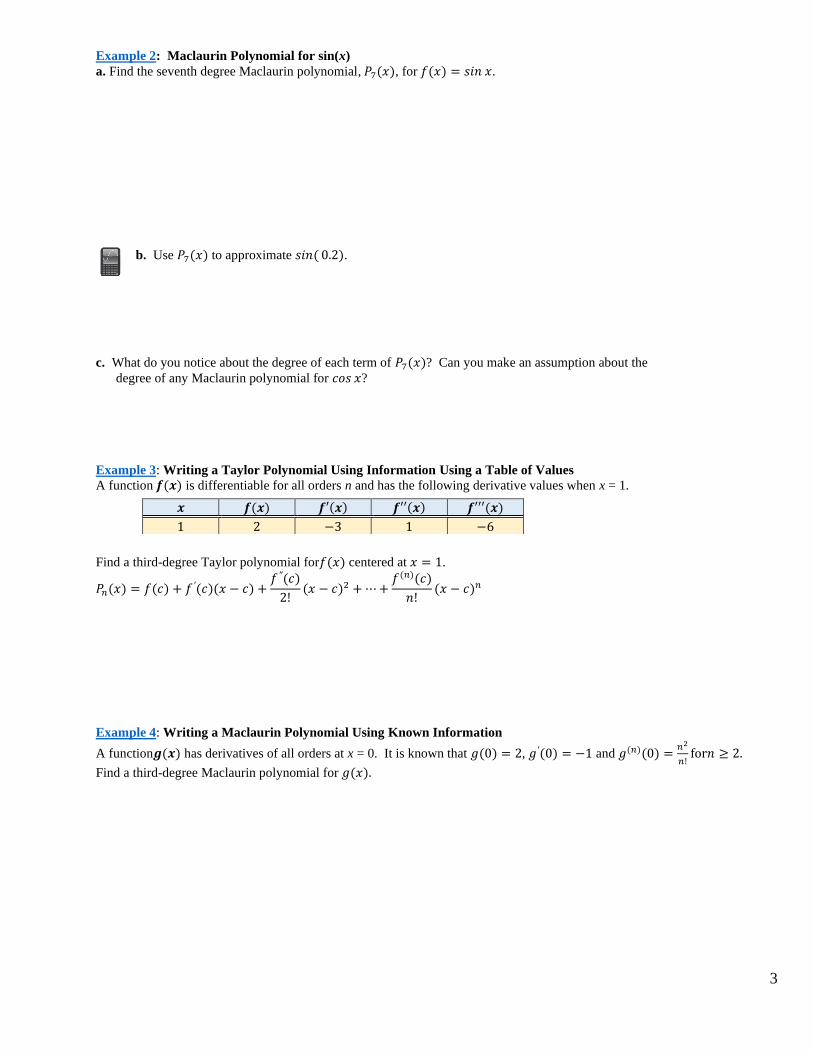
Example 2: Maclaurin Polynomial for sin(x)

a. Find the seventh degree Maclaurin polynomial, 𝑃7(𝑥), for 𝑓(𝑥) = 𝑠𝑖𝑛 𝑥.

b. Use 𝑃7(𝑥) to approximate 𝑠𝑖𝑛( 0.2).

c. What do you notice about the degree of each term of 𝑃7(𝑥)? Can you make an assumption about the

degree of any Maclaurin polynomial for 𝑐𝑜𝑠 𝑥?

Example 3: Writing a Taylor Polynomial Using Information Using a Table of Values

A function 𝒇(𝒙) is differentiable for all orders n and has the following derivative values when x = 1.

Find a third-degree Taylor polynomial for𝑓(𝑥) centered at 𝑥 = 1.

𝑃𝑛(𝑥) = 𝑓(𝑐) + 𝑓 ′(𝑐)(𝑥 − 𝑐) +𝑓″(𝑐)

2!(𝑥 − 𝑐)2 + ⋯ +

𝑓(𝑛)(𝑐)

𝑛!(𝑥 − 𝑐)𝑛

Example 4: Writing a Maclaurin Polynomial Using Known Information

A function𝒈(𝒙) has derivatives of all orders at x = 0. It is known that 𝑔(0) = 2, 𝑔′(0) = −1 and 𝑔(𝑛)(0) =𝑛2

𝑛!for𝑛 ≥ 2.

Find a third-degree Maclaurin polynomial for 𝑔(𝑥).

𝒙 𝒇(𝒙) 𝒇′(𝒙) 𝒇′′(𝒙) 𝒇′′′(𝒙)

1 2 −3 1 −6

4

One of the primary goals of studying Taylor Polynomials and, later in Topic 10.14, Taylor Series is to find a way to represent an

“ugly” function as a “prettier” function that we can manipulate much easier.

The focus for this topic will be to investigate how close our Taylor approximations are to the actual value of the function.

The Remainder of a Taylor Polynomial 𝒇(𝒙) = 𝑷𝒏(𝒙) + 𝑹𝒏(𝒙)

𝑷𝒏(𝒙

The remainder will serve as the error in our approximation, therefore, Error =|𝑹𝒏(𝒙) = |𝒇(𝒙) − 𝑷𝒏(𝒙)||

The theorem below gives a general procedure for estimating the remainder associated with a Taylor polynomial.

The theorem, often called Taylor’s Theorem defines a remainder that, when isolated, is referred to as the

Lagrange form of the remainder or the Lagrange error bound.

LIM AP CALCULUS BC

1 Topic: 10.12 Lagrange Error Bound

Learning Objectives LIM-8.C: Determine the error bound associated with a Taylor polynomial approximation.

Exact

Value

Approximate

Value

Remainder

THEOREM 10.12.1 TAYLOR’S FORMULA &

LAGRANGE ERROR BOUND

If a function f is differentiable through order n + 1 in an interval, I, containing c, then,

for each x in I, there exists z between x and c such that

𝑓(𝑥) = 𝑓(𝑐) + 𝑓 ′(𝑐)(𝑥 − 𝑐) +𝑓″(𝑐)

2!(𝑥 − 𝑐)2 + ⋯ +

𝑓(𝑛)(𝑐)

𝑛!(𝑥 − 𝑐)𝑛 + 𝑅𝑛(𝑥)

where

|𝑅𝑛(𝑥)| = ቚ𝑓(𝑛+1)(𝑧)

(𝑛+1)!(𝑥 − 𝑐)𝑛+1ቚ.

5

Example 1: Determining the Accuracy of the Approximation

The third Maclaurin polynomial for 𝑠𝑖𝑛 𝑥 is given by 𝑃3(𝑥) = 𝑥 −𝑥3

3!.

Use Taylor’s Theorem to approximate 𝑠𝑖𝑛( 0.1) by 𝑃3(0.1) and determine the accuracy of the approximation.

Example 2: Finding the Range of Possible Values for an Approximation

Find the third-degree polynomial approximation for 𝑒𝑥 at x = 1, centered at 0. Use Taylor’s Inequality to find the range of

possible values for𝑒𝑥at x = 1, centered at 0.

Example 3: Approximating a Value to a Desired Accuracy

Determine the degree of the Taylor polynomial Pn(x) expanded about c = 1 that should be used to approximate 𝑙𝑛( 1.2) so that

the error is less than 0.001.

TAYLOR’S INEQUALITY

Often we can represent the error as a bound using the inequality

|𝑅𝑛(𝑥)| ≤ ฬ𝑚𝑎𝑥ൣ𝑓(𝑛+1)(𝑧)൧

(𝑛+1)!(𝑥 − 𝑐)𝑛+1ฬ.

The notation maxൣ𝑓(𝑛+1)(𝑧)൧ represents the largest value 𝑓(𝑛+1)(𝑧) will

take on for a z that will (typically) lie between c and x.

TIP

When f(x) = sinx or cosx,

the value for the max of

f(n+1)(z) will always be 1.

6

Power Series Goal: Show how an infinite polynomial function can be used as an EXACT expression for other elementary

functions.

For example: The function 𝑓(𝑥) = 𝑒𝑥can be represented exactly by

𝑒𝑥 = 1 + 𝑥 +𝑥2

2!+

𝑥3

3!+ ⋯ +

𝑥𝑛

𝑛!+ ⋯ We call this a power series.

For each real number, x, it can be shown that the infinite series on the right converges to the value 𝑒𝑥.

Example 1: Power Series

State the value of c where each power series is centered.

a. ∑𝒙𝒏

𝒏!

∞𝒏=𝟎 b. 𝟏 − (𝒙 + 𝟏) + (𝒙 + 𝟏)𝟐 − (𝒙 + 𝟏)𝟑 + ⋯ c. ∑

𝟏

𝒏(𝒙 − 𝟏)𝒏∞

𝒏=𝟎

LIM AP CALCULUS BC

2 Topic: 10.13 Radius and Interval of convergence of Power Series

Learning Objectives LIM-8.D: Determine the radius of convergence and interval of convergence for a power series.

DEFINITION OF POWER SERIES

If x is a variable, then an infinite series of the form

𝑎𝑛𝑥𝑛

∞

𝑛=0

= 𝑎0 + 𝑎1𝑥 + 𝑎2𝑥2 + 𝑎3𝑥3 + ⋯ 𝑎𝑛𝑥𝑛 + ⋯

is called a power series. More generally, an infinite series of the form

𝑎𝑛(𝑥 − 𝑐)𝑛

∞

𝑛=0

= 𝑎0 + 𝑎1(𝑥 − 𝑐) + 𝑎2(𝑥 − 𝑐)2 + 𝑎3(𝑥 − 𝑐)3 + ⋯ 𝑎𝑛(𝑥 − 𝑐)𝑛 + ⋯

is called a power series centered at c, where c is a constant.

7

Radius and Interval of Convergence

Think of a power series as a function of x like

𝑓(𝑥) = ∑ 𝑎𝑛(𝑥 − 𝑐)𝑛∞𝑛=0

where the domain of f is the set of all x for which the power series converges.

Determining the domain of a power series is the primary concern of this section.

Note: A power series converges at its center c because

𝑓(𝑐) = 𝑎𝑛(𝑐 − 𝑐)𝑛 = 𝑎0(1) + 0 + 0 + 0 + ⋯ + 0 + ⋯ = 𝑎0

∞

𝑛=0

So, c always lies in the domain of f

Example 2: Finding the Radius of Convergence

Find the radius of convergence for each power series.

a. ∑ 𝒏! 𝒙𝒏∞𝒏=𝟎 b. ∑ 𝟑(𝒙 − 𝟐)𝒏∞

𝒏=𝟎

Find the radius of convergence for each power series.

c. ∑(−𝟏)𝒏𝒙𝟐𝒏+𝟏

(𝟐𝒏+𝟏)!

∞𝒏=𝟎

THEOREM 10.13.1 CONVERGENCE OF A POWER SERIES

For a power series centered at c, precisely one of the following is true.

1. The series converges only at c.

2. There exists a real number R > 0 such that the series converges absolutely for

|𝑥 − 𝑐| < 𝑅, and diverges for |𝑥 − 𝑐| > 𝑅.

3. The series converges absolute for all x.

The number R is called the radius of convergence of the power series. If the series converges only at c, the radius

of convergence is R = 0, and if the series converges for all x, the radius of convergence is R = ∞.

The set of all values of x for which the power series converges is the interval of convergence of the power series.

The 3 Types of Convergence of a

Power Series

8

Endpoint Convergence

Note that for a power series whose radius of convergence is a finite number R, the theorem above says nothing about the

convergence at the endpoints of the interval of convergence. Each endpoint must be tested separately for convergence or

divergence. Therefore, the interval can take any one of the following six forms:

Example 3: Finding the Interval of Convergence

Find the interval of convergence for each power series.

a. ∑𝒙𝒏

𝒏

∞𝒏=𝟏

b. ∑(−𝟏)𝒏(𝒙+𝟏)𝒏

𝟐𝒏∞𝒏=𝟎

c. ∑𝒙𝒏

𝒏𝟐∞𝒏=𝟏

9

Differentiation and Integration of Power Series All of the “founding fathers” of calculus, Newton, Leibniz, Euler, Lagrange, and the Bernoulli brothers used power series

extensively in their individual development of the subject.

Because of this, one can only wonder are power series continuous? Are they differentiable?

Can we integrate a power series?

THEOREM 10.13.2 PROPERTIES OF FUNCTIONS DEFINED BY POWER SERIES

If the function given by

has radius of convergence of R > 0, then, on the interval (c – R, c + R), f is differentiable (and

therefore continuous). Moreover, the derivative and antiderivative of f are as follows:

1.

2.

The radius of convergence of the series obtained by differentiating or integrating a power series is the same as that

of the original power series. The interval of convergence, however, may differ as a result of the behavior at the

endpoints.

10

Example 4: Intervals of Convergence for f(x), f'(x), and ʃ f(x)dx

Consider the function given by 𝑓(𝑥) = ∑𝑥𝑛

𝑛= 𝑥 +

𝑥2

2+

𝑥3

3+ ⋯ .∞

𝑛=1 .

Find the interval of convergence for each of the following.

a. 𝒇(𝒙) b. 𝒇′(𝒙) c. ∫ 𝒇(𝒙)𝒅𝒙

Activity:

1. Given 𝑓(𝑥) = ∑𝑥𝑛

𝑛!

∞𝑛=0 , write out an expression that includes the first five terms of the series.

2. Find 𝑓 ′(𝑥) by differentiating the terms in the series above.

3. What do you notice about𝑓(𝑥) and𝑓 ′(𝑥)? Do you recognize this function?

11

Taylor and Maclaurin Series

Example 1: Maclaurin Series and Convergence

Find the Maclaurin series, in summation form, for the following functions. Find the interval of convergence for each series as

well.

a.) 𝒇(𝒙) = 𝒄𝒐𝒔 𝒙 Video 1a

Find the Maclaurin series, in summation form, for the following functions. Find the interval of convergence for each series as

well.

b.) 𝒇(𝒙) =𝟏

𝟏−𝒙 Video 1b

LIM AP CALCULUS BC

2 Topic: 10.14 Finding Taylor or Maclaurin Series of a Function

Learning Objectives LIM-8.E: Represent a function as a Taylor series or a Maclaurin series. LIM-8.F: Interpret Taylor series and Maclaurin series.

THEOREM 10.14 THE FORM OF A CONVERGENT POWER SERIES

If f is represented by a power series for all x in an open interval I,

containing c, then and

𝒇(𝒙) = 𝒇(𝒄) + 𝒇′(𝒄)(𝒙 − 𝒄) +𝒇″(𝒄)

𝟐!(𝒙 − 𝒄)𝟐 + ⋯

𝒇(𝒏)(𝒄)

𝒏!(𝒙 − 𝒄)𝒏 + ⋯

DEFINITION OF TAYLOR AND MACLAURIN SERIES

If a function f has derivatives of all orders at , then the series

is called the Taylor series for f(x) at c. Moreover, if c = 0, then the series is the Maclaurin

series for f(x).

12

The following table lists important information about some of the most popular power series encountered in calculus. You are

strongly encouraged to memorize the series marked with a as they are commonly featured on the AP Calculus BC exam.

* The convergence at x = ±1 depends on the value of k.

Function First Four Terms General Term Interval of

Convergence

1

𝑥

1 − (𝑥 − 1) + (𝑥 − 1)2 − (𝑥 − 1)3 + ⋯ (−1)𝑛(𝑥 − 1)𝑛 0 < 𝑥 < 2

1

1 + 𝑥

1 − 𝑥 + 𝑥2 − 𝑥3 + ⋯ (−1)𝑛𝑥𝑛 −1 < 𝑥 < 1

𝑙𝑛 𝑥 (𝑥 − 1) −(𝑥 − 1)2

2+

(𝑥 − 1)3

3−

(𝑥 − 1)4

4

(−1)𝑛−1(𝑥 − 1)𝑛

𝑛 0 < 𝑥 ≤ 2

𝑒𝑥 1 + 𝑥 +𝑥2

2!+

𝑥3

3!+ ⋯

𝑥𝑛

𝑛! −∞ < 𝑥 < ∞

𝑠𝑖𝑛 𝑥 𝑥 −𝑥3

3!+

𝑥5

5!−

𝑥7

7!+ ⋯

(−1)𝑛𝑥2𝑛+1

(2𝑛 + 1)! −∞ < 𝑥 < ∞

𝑐𝑜𝑠 𝑥 1 −𝑥2

2!+

𝑥4

4!−

𝑥6

6!+ ⋯

(−1)𝑛𝑥2𝑛

(2𝑛)! −∞ < 𝑥 < ∞

𝑎𝑟𝑐𝑡𝑎𝑛 𝑥 1 −𝑥3

3+

𝑥5

5−

𝑥7

7+ ⋯

(−1)𝑛𝑥2𝑛+1

2𝑛 + 1 −1 ≤ 𝑥 ≤ 1

𝑎𝑟𝑐𝑠𝑖𝑛 𝑥 𝑥 +𝑥3

2 ⋅ 3+

1 ⋅ 3𝑥5

2 ⋅ 4 ⋅ 5+

1 ⋅ 3 ⋅ 5𝑥7

2 ⋅ 4 ⋅ 5 ⋅ 7+ ⋯

(2𝑛)! ⋅ 𝑥2𝑛+1

(2𝑛𝑛!)2(2𝑛 + 1) −1 ≤ 𝑥 ≤ 1

(1 + 𝑥)𝑘 1 + 𝑘𝑥 +

𝑘(𝑘 − 1)𝑥2

2!+

𝑘(𝑘 − 1)(𝑘 − 2)𝑥3

3!+ ⋯

𝑘(𝑘 − 1)(𝑘 − 2) ⋯ (𝑘 − (𝑛 − 1))𝑥𝑛

𝑛! −1 < 𝑥 < 1 *