TRACIVB PROFESSIONAL SURVEY SYSTEMS

Mobilise in hours with no performance risk using Oubit's TRAC IV B Survey Systems! Hundreds of completed contracts and satisfied clients testify to an unrivalled capability for delivering on time and to specification. Trac systems for:-Hydrographic Survey: used and accepted for Ministry of Defence work since1983. Pipeline ROV Survey: to Shell and Statoil specification since 1981. Barge work: on cross channel cable project for CEGB since 1982, are just some of Oubit's quiet achievements. TRAC IV B not only provides all real-time functions, the interfacing and integration of survey data, operator displays and logging information, - but also complete on board processing of data. Thus reports and fair chart drawings can be completed within hours.

The ruggedised compact systems are easily shipped and installed. Operators find them effective and friendly, making for efficient vessel and equipment operation. Reports and drawings can be finalised on-board and fast response for systems, spares or support is our business. Contact Qubit for a survey system as tough as your contract

IIIII I IIIII I

4\IBiT

Qubit UK Limited 251 Ash Road Aldershot Hampshire GI,J12 400 Telephone (0252) 331418 Telex 858593 OUBIT G Qubit Pty Limited 18 Prowse Street West Perth Western Australia 6005 Telephone (09) 322 4955 Telex AA93960

EDITION NO. 31 LIGHTHOUSE MAY, 1985

JOURNAL OF THE CANADIAN HYDROGRAPHERS' ASSOCIATION

National President .. . ........ .. ... ... .. ..... ........ . . . .. J. Hruce Secretary-Treasurer ...... ... . . .... . . . ... . . . ... . ... ... .. S. Acheson Vice-President, Atlantic Branch ...... ..... ... .... ... . ... R. Mehlman Vice-President, Ottawa Branch . ..... . ......•.... ... •. . . . T. Tremblay Vice-President, Central Branch ... ... · ................. .. . . . . D. Pugh Vice-President, Pacific Branch . . .............. .. ............ B. Lusk Vice-President, Quebec Branch . .. . .. . ..... . ..... .. ... ... P. Bellemare Vice-President, Prairie Schooner Branch . .... .. ....... ..... H. Stewart

Edi10rial Siaff

Editor . . .. ..... .. .... . . ... .... Rear Admiral D.C. Kapoor Assistant ·Editors ...... . . .. .. . . ... ........ . .... A.J. Kerr

. . . . . . . . . . . . . . . . . . . . . . . . S. W Sandi lands

........... ....... . ...... . . D. Monahan

.... .. . .. . ................ G. Macdonald Social News Editor ......... . ..... . ... . .... .... .. D. Pugh Advertising Manager .............. . . ..... . . ... Dr. A Baud Graphics ..... . ... . ..... .. ...... . . ...... . F inancial Manager . . . . . . . . . . . . . . . . . . . . . . . . . . Dr. A. Baud

LIGHTHOUSE is published twice yearly by the Canadian Hydrographers' Association and is distributed free to its members. Yearly subscription rates for non members who reside in Canada are $10. For all others $15, payable by cheque or money order to the Canadian Hydrographers Association.

All correspondence should be sent to the editor of LIGHT­HOUSE, c/o Canadian Hydrographers Association, P.O. Box 5378, Station "F", Ottawa, Ontario, Canada, K2C 3JI.

LIGHTHOUSE Advertising Rates Per Issue

Outside Back Cover . . . .. ..... . . . ........... $180.00 CAN. Inside Cover, Page ... . . .• ...... . ....... .. ..... . .. $170.00 Half Page ..... . ... . ... . ... : ... .. . . ... . ...... .. . $115.00

Body, Full Page ....... .• ...... . •...... .. ........ $155.00 HalfPage . .. .... . . .. . ... ... . .. ...... . ..... ... . . $100.00 Quarter Page .. . . . . . . ...... . ... . ....... ... ..... .. $80.00

Professional Card .. ..... . . .... ... . ...... ... .. . . . .. $45.00 Single-Page Insert . . . .. . .... . . .... .. ........ . . . . . $155.00 Color rates available on request

All Rates Net To Publisher

Closing Dates: April Issue - I March November Issue - I October

For a rate card and mechanical specifications contact:

Editor, LIGHTHOUSE Canadian Hydrographers Association

P.O. Box 5378, Station "F" Ottawa, Ontario, Canada

K2C 311

Contents Page

An Opinion Computer Assitance . . . . . . • . . . . . . . . . . . . . . • . . . . • . . . . . . . . . . . . . 3 Adam J . Kerr

Evaluation of The QUBIT TRAC IV 8 ..... . .... • .. . .• . . . ..... 5 H.P. Varma

The Use of Sea Level Tide Gauge Observations in Geodesy . ... . .......... • .•.. . . . .... ... ..... 13 Gala Carrera and Petr Vanicek

The Hydrographic Contouring System Practical Experiences . . . . . . . . . . . . . . . . . . . . • . . . . . . . . . . . . . . . . . 20 Dan McDonald and Carl Czotter

Next Generation Plotters ... .. . ... . ..• . . . .. ...... . ..• ....... 24 Don H. Vachon

Views expressed in articles appearing m this publication are those of the authors and not necessarily those of the Association.

I·

PORTABLE SPARKER SYSTEM -for-

NEAR SHORE ENGINEERING SURVEYS

PROVIDES HIGH RESOLUTION SEISMIC PROFILES • Marine foundations surveys • Submarine pipeline surveys • Sand and gravel inventory • Mineral prospecting Ultra small size and light weight. Can be used on very small boats.

• Hazard surveys • Pre-dredge investigation • Bedrock contours • Bore hole tie in

Product data plus sample recordings sent upon request. SALE AND LEASE

THE BEST OF BOTH WORLDS FORMANCE • PRICE ·

The INNERSPACE Model 431 Acoustic Release

• Reasonable price. • Many codes (80 codes max.). • Secure coding. • Small size (28" long - SY." Dia.). • Light weight (6 lbs. in water). • Safe, no exploding devices. • Inexpensive, replaceable batteries. • Optional rope canister. • Optional load multiplier.

The Model 431 is designed spt!cifically for shallow waterapplications (to 1000 ft.) for the recovery of in situ instruments - trans­ponders, current meters,lapsed time cameras and is ideal for relocating underwater sites - well heads, valves, cables, submersibles, etc.

THERMAL DEPTH SOUNDER RECORDER FOR PRECISION MARINE SURVEYS

FIXED HEAD THERMAL PRINTING - NO STYLUS CLEAN, QUIET, ODORLESS

SCALE LINES/DEPTH ARE PRINTED SIMULTANEOUSLY ON BLANK PAPER

ONLY CHART SCALE SELECTED IS PRINTED

• Chart Paper - 8'12 inches x 200 feet (blank thermal paper).

• Depth Ranges- 0.320 feet/fathoms and 0.145 meters (7 phases). Plus X2 and X10 all ranges.

• Fri!C!uencles (2)-208 kHz, and 41 kHz, 33kHz, 28kHz or 24kHz.

• Data Entries- Digital thumbwheels for speed of sound, tide and draft.

• Annotation Generator- Numerically prints speed of sound, tide and draft on chart.

• Custom Logo ROM - Prints customer logo and name on chart.

• Precision Depth Digitizer- Auto Track Model 441 -features auto bottom tracking gate, auto selection of recorder depth range. BCD output plus optional RS232C or IEEE488-GPIB outputs.

• Multiple Transducer System-option Model 442- provides for 3 to 6 channel swath surveys. ·

• Deep Water Projects-proven 2000 meters capability using 24 kHz.

I• I I INNERSPACE TECHNOLOGY, INC.

ONE BOHNERT PLACE • WALDWICK, NEW JERSEY 07463

(201) 447-0398 TWX 710-988-5628

ll MODEL 440 TDSR

An Opinion Computer Assistance

Does It Increase Hydrographic Productivity? by Adam J. Kerr

Computers were first used in hydrography for geodetic computa­tions and indeed that is still one of their main functions. During the last twenty years computers have been progressively used for more and more hydrographic operations but it still remains an open question as to whether or not they increase product ivity or· whether they are cost effective. This author gives a qualified "yes" to the first of these and leaves the latter as an open question.

It is difficult to justify the need for computers by themselves but they permit other instruments and methods to be gainfully used. We can simply divide surveying into two main areas: data collec­tion and data processing. Many people see computer advantages primarily in data processing but unless data can be collected more rapidly we can process as fast as we like and the productiv­ity will not increase unless there was initially a bottleneck due to slow manual processing.

Let us look at the data collection phase and see how computers can help. During the nineteen sixties several national hydrogra­phic offices, including Canada, started introducing comp4ters and automatic plotting systems at sea on larger ships. We were excited by the technology but it did not increase the productivity. The ships still travelled at 12 or so knots and in fact it was the introduction of elect ronic positioning systems and possibly improved sounding systems, such as the ram transducer, that helped to increase productivity. Computers did hav,e a place on ships at this time and this was to carry out on-line processing of geophysical data - but they did not increase the productivity. However, it was found that computers and plotters did have a place for operations that were slow and difficult by manual means. One of these was the plotting of hyperbolic lattices. This was a very tedious business by hand. The other was the plotting of projections which also tended to be time consuming. ThesP. two tasks were required for both the field hydrography and the chart production and consequently the introduction of computers and peripherals was clearly a step towards increased productivity.

It was in the survey launch operation that computers really showed potential but few hydrographic offices followed th is lead, possibly because the hardware costs were high and the software development demanding. Until the nineteen sixties survey launches had normally sounded at slow speeds of around 8 knots. After all, bobbing up and down taking sextant angles and plotting them underway took at least a minute for each fix and if you do not go too fast you will not find yourself too far off the line between fixes. But electronic positioning systems which were miniature and more accurate versions of the offshore Decca were becoming available and these could provide a fix as fast as you could read the dials, provided you had the reference lattice previously men­tioned. Furthermore, if you kept one reading constant you could run a systematic set of concentric or hyperbolic lines and as far as line keeping was concerned the speed of the lauch was not a problem. There did, however, remain a difficulty; this was the precise correlation of the depth measurement with the position. This difficulty was overcome by electronics which annotated the echo sounding graph at precise cyclic readings of one elect ron ic positioning pattern. Finally we were able to sound faster and accurately, although we had to take care that the pulse rate was sufficiently high that no gaps were left along the track. So even without the computer it was the combined introduction of elec-

Lighthouse: Edition No. 31 , May, 1985

tronic positioning with higher speed launches that increased the productivity.

During the late nineteen sixties launch data logging systems were introduced. The earlier versions were hard-wi red but neverthe­less we were able to correlate time, position and depth and store it on a computer readable medium (punch paper tape and paper magnetic tape). This was the ultimate but it needed a computer at hand to process the data. Some people felt that it might be possible to process all the data at some central point but the need to know w ith in 24 hours how the data " looked" meant that realisti­cally computers had to go in the field .

The introduction of lower cost mini-computers soon allowed hydrographers to consider the use of computers as part of the on-line operation. It was now possible to rectify the peculiar coordinates of the positioning systems into some convenient rectangular system such as UTM or geographic coordinates and from here it was but a step further to calculate offsets f rom a chosen straight line track and to provide this as steering indica­tions on a meter in front of the helmsman. This presented a significant increase in productivi ty and convenience because the hyperbolic position lines wh ich typically resulted from several positioning systems were not paral lel and the hydrographer had to adjust his survey to make the best use of the pattern. The rectilinear position lines allowed a more systematic and effective coverage of the survey area and hence a greater economy.

The ultimate in hands off technology for ship, launch and even aircraft was the linkage of the positioning system to the steering of the vehicle. It is questionable if this really results in increased productivity but it does ensure that course steering can be syste­matic and without humanly induced steering errors. Carried to the extreme this type of technology allows a whole block of parallel survey lines to be steered under complete computer control. An early example of this using a hard-wired computer was Decca's Survey Marine Sidewal l Hovercraft System, in use in the late sixties. But once again, the system was fascinating to watch but it did not survey faster nor did it release surveyors or crew for other work.

The fact that the combination of electronic positioning, faster survey vessels and computers to correlate the data has resulted in more data being collected has not been without its cost in other directions. There has been an increased need for elect ronic tech­nicians and computer specialists. If resources remain finite it means that these personnel must be taken from the ranks of those who normally are out there col lecting the data. If, though , resour­ces have not remained stationary but the number of collecting vessels has been constrained, then the productivity has been able to increase.

So we have found ways to collect more data but now we are left with a bottleneck at the processing. Before faster launches and electronic positioning, a survey party could general ly keep up with the data processing by making use of bad weather days to scale the echo sounding graphs and to plot the data. If the weather remained fine it may f rom time to time have been neces­sary to hold one or two of the survey launches back to provide personnel for data processing. But this seldom happened, partie-

Page3

i·

ularly in the Arctic, where a "good blow" could be expected with some regularity.

Today the pace of data collection would overwhelm the capability of the average survey party to process it without the help of a computer. The computerfirstcomes into its own in quickly calcu­lating the geodetic positions. At one time surveyors would work late into the night getting "geodetics" calculated before the sounding could start and time would often be lost while the control was computed and plotted. Th is problem has been removed and "canned" programs are readily available to quickly calculate the control. Once the sounding is underway, computer processing becomes an essential part of the operation and th is relieves the potential bottleneck. While it is true that some small survey parties can carry on with manual processing and hand inking, a fully fledged modern survey can on ly be productive when equipped with computer systems both aboard the launches and at the field processing centre. The use of a computer w il l permit the data from one day to be processed overnight in time to make program decisions for the next day. Clever uses of the field computer allow the hydrographer-in-charge to optimize deploy­ment of the survey vehicles. This in all probability also helps to increase the overall productivity.

Although hydrographers are becoming yearly more familiar with computer-assisted methods of hydrographic surveying, they remain , in many cases, frustrated by a high level of software bugs. The problem is somewhat circular as the more they use the system the more intricate and complex are the things they demand from the systems. The result of this is the real reason for computerizing the field surveys. Unfortunately, at this time there is a hiatus or "missing link" in the process. Until we can find the link this argument does not hold.

In answering the question "Are Computers Allowing Us To Be More Productive in Hydrography?", the answer is a qualif ied "yes" but the quest ion whether computers are permitting us to be economically cost effective requires more careful consideration. There is some difficulty in answering this question because some additional start-up costs have been inevitable. In the twenty or so years that computers have been used there has undoubtedly been a lot of money poured into the development of an effective system but now that we have one- and this may be considered contentious by some- are we cost effective? This remains an open question.

PRECISION SURVEYING

Page4

with Mesotech Deep Diving ECHO SOUNDERS

Pressure-proof to 6600 ft.

NO OTHER SONAR COMES CLOSE

MESOTECH SYSTEMS LTD 2830 Huntington Place,

• Remove Water­Column Errors

• Increase Range ·Resolution

• Construct Swath Arrays

• Characterise Bottom (809)

• Modei807-Analog output

• Model 80S­Digital output

• Modei809-Programmable

Port Coquitlam, B.C , Canada V3C 4T3 Telephone: (604) 464-8144 Telex: 04-353637

Lighthouse: Edition No. 31, May, 1985

EVALUATION OF THE QUBIT TRAC IV 8 by

H.P. VARMA

Canadian Hydrographic Service (Atlantic Region) Department of Fisheries and Oceans Bedford Institute of Oceanography

P.O. Box 1006 Dartmouth , Nova Scotia

B2Y 4A2

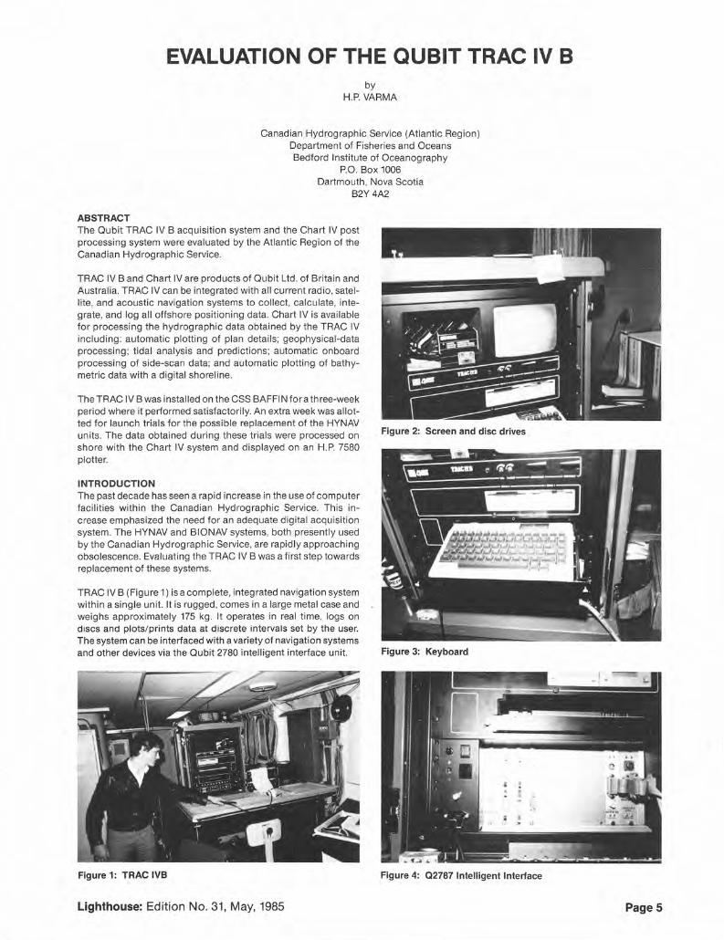
ABSTRACT The Oubit TRAC IV B acquisition system and the Chart IV post processing system were evaluated by the Atlantic Region of the Canadian Hydrographic Service.

TRAC IV Band Chart IV are products of Qubit Ltd. of Britain and Australia. TRAC IV can be integrated with all current radio, satel­lite, and acoustic navigation systems to collect, calculate, inte­grate, and log all offshore positioning data. Chart IV is available for processing the hydrographic data obtained by the TRAC IV including: automatic plotting of plan details; geophysical-data processing; tidal analysis and predictions; automatic onboard processing of side-scan data; and automatic plotting of bathy­metric data with a digital shoreline.

The TRAC IV B was installed on the CSS BAFFIN for a three-week period where it periormed satisfactorily. An extra week was allot­ted for launch trials for the possible replacement of the HYNAV units . The data obtained during these trials were processed on shore with the Chart IV system and displayed on an H.P. 7580 plotter.

INTRODUCTION The past decade has seen a rapid increase in the use of computer facilities with in the Canadian Hydrographic Service. This in­crease emphasized the need for an adequate digital acquisition system. The HYNAV and BIONAV systems, both presently used by the Canadian Hydrographic Service, are rapidly approaching obsolescence. Evaluating the TRAC IV B was a first step towards replacement of these systems.

TRAC IV B (Figure 1) is a complete, integrated navigation system within a single unit. It is rugged, comes in a large metal case and weighs approximately 175 kg. It operates in real time, logs on discs and plots/ prints data at discrete intervals set by the user. The system can be interfaced with a variety of navigation systems and other devices via the Qubit 2780 intelligent interface unit.

Figure 1: TRAC IVB

Lighthouse: Edition No. 31, May, 1985

Figure 2: Screen and disc drives

Figure 3: Keyboard

Figure 4: 0 2787 Intelligent Interface

Page 5

EVALUATION The TRAG IV B system was evaluated for one week by the Cana­dian Hydrographic Service as a possible replacement for the HYNAV unit. It was installed aboard the Canadian survey vessel NAVICULA, in the Bedford Basin. The positioning systems util­ized were a Miniranger with four transponders, and Loran-C. An ELAC echo sounder was interfaced to the unit via an ELAC STG 721 digitizer.

The TRAG IV B was also aboard CSS BAFFIN for three weeks in case it was needed to replace BIONAV (the Bedford Institute of Oceanography navigation system).

SYSTEM DESCRIPTION The TRAG IV B has six major components: (1) a storage com­partment and monitor, (2) a dual disc drive unit, (3) a keyboard (removable), (4) a microcomputer, (5) interfacing connections, and (6) power requirements.

(1) The storage compartment is located at the top left of the front panel (Figure 2). It can be used to store auxiliary cables, manuals, and also accessory kits. The monitor is a mono­colour graphic display unit with an 'anti-reflective' screen. It is switched on automatically when power is supplied to the TRAG IV B.

(2) The dual disc drive un it is to the centre right of the front panel and is switched on immediately when power is supplied to the TRAG IV B. The drive is automatically activated by inserting the microdiscs into the units. At present, each disc has the limited storage capability of half a megabyte. The disc may be ejected by pushing the square button on the disc drive.

(3) The keyboard is located towards the centre of the front panel (Figure 3), and may be accessed by undoing the two thumb­screws on either side of the keyboard's front panel, then withdrawing the sliding tray. It is ful ly operational in this position, and all function keys are accessible. The keyboard can also be fully withdrawn from the cabinet on its cable for remote use.

(4) The TRAG IV is currently based on the Hewlett Packard 9920 computer system. The software is written in PASCAL, BASIC, and ASSEMBLER. The TRAG IV also has thecapability to run on the Hewlett Packard 9816/26/36 systems, thus increasing its computer options.

(5) The TRAG IV B incorporates a 02787 (Figure 4) smart inter­face module capable of interfacing up to 10 devices. The 02787 is interfaced to an H.P. 9920 via Hewlett Packard Inter­face Bus I EEE-488; however, provision has been made for the fitting of "serial connectors." This option can be obtained f rom the Oubit company.

(6) The present power requirements for the TRAG IV B are 230V/115V A.C. These options can be selected with the "V.SEL" switch on the front panel

SOFTWARE The bu lk of the software available for the system is modular and written in BASIC in order to facilitate the ed iting and mod ification of existing software. The prog rams were then translated into PASCAL to further increase the execution speed. The 1/ 0 drivers were written in ASSEMBLER CODE by the OUBIT company because they were not available from Hewlett Packard . The data structure of the system incorporates 20 lines of position in raw format , computed position , Gyro bearing, and ten stacked soundings.

Position computations were computed every 2 seconds, and then depicted on the graphic display units. The logging rate on disc was about once every 4 seconds. The relatively long time interval between position computations was of concern to our hydrogra­phic f ield personnel, but Oubic has assured us that this rate can be significantly increased in the seismic mode.

PageS

Chart IV is a post processing system designed to read disc data that has been accumulated by the Oubit TRAG IV B system. It can apply tide corrections and allows sounding selection and interac­tive editing techniques on depth profiles (Figure 5). It can also provide plotting facilities on an H.P. 7580 plotter to produce track plots (Figure 6), (Figure 7), and plot bathymetry (Figure 8), (Fig­ure 9). The system provides a number of facilities, including; the ability to back up the raw data logged in the field; edit the naviga­tional parameters used in the determination of position; convert the raw data to XYZ data; and edit 'run line' libraries and data base files.

RESULTS Several groups of Atlantic fie ld personnel participated in run ning the TRAG IV, gaining hands-on experience. The results of the testing of OubitTRAC IV B on the NAVICULA were discussed in a meeting between Oubit personnel and field hydrographers on December 6, 1984, at the Bedford Institute of Oceanography.

The first problem d iscussed was the position computat ion t ime factor of 2 seconds. The Canadian Hydrographic Service requires faster updates for high-speed launch su rveys and helicopter su r­veys. The helicopter requires an acquisit ion system for logg ing a dig ital shoreline at speeds in excess of 100 km/ h. Oubit said that their seismic mode would provide an option for faster updates and therefore could solve this problem.

The second problem was that the posit ion computation was exe­cuted in plane co-ordinates ('Northing' and 'Easting') and then converted into 'Geographies'. This poses a major problem for the Canadian Hydrographic Service since many areas such as Sable Island, Foxe Basin, and Jones Sound field sheets straddle UTM Zones. If computations are done in Geograph ies one can then calculate the Zone. If done in plane co-ordinates, the Zone can­not be derived but must instead be entered manual ly. If computa­tions continue into adjacent Zones util izi ng previous Zone values, erroneous Geographic Values are logged. Because our launches often cross from one Zone to another, especially at Zone peri­pheries, this problem would pose major diffi culties in post pro­cessing of data.

The third problem raised was that there was no weighting LOPs. This weighting cou ld be done in accordance to d istance from stations or the respective positioning systems, signal to noise ratio, all with a manual override capabi lity.

Ann ther question raised by the field personnel related to the 10-to-1 5 second lag in the update of the Graphic Display Screen. This delay would cause one of our high speed launches to veer off line since the Ship's Coxwain would be steering by dead reckon­ing. The possibil ity to 'grid' the sc reen and refresh localized sections could significantly cut the display lag.

There was a consensus among the field and development per­sonnel that the Oubit TRAG IV package should be reduced in both size and weight. This point was emphasized so that the system could be made portable for hel icopter, launch, or car uti I ity. The system is too large, heavy and unwieldy for one person to manage easily. Oubit is considering the idea of splitting the box into two units, wh ich would increase the system's po rtability.

Another problem raised was the limited storage capacity of the discs. Half a megabyte would not be enough storage for high­speed launch surveys. This would lead to a multitude of discs on each launch. Hard discs or streaming cartridges would be a better logging alternative because they would reduce the number of removable discs required.

There were also comments about replacing the keyboard with a

Lighthouse: Edition No. 31 , May, 1985

i·

~

f-5~

··-.. r-··-r· r·-..... L-1 ..... r---.... T.-·" ··.

... ·.

1-H 0 't-.. ·1-·

~;CRLE 1 . 15 P~J0 5 . Figure 5

BAFFIN 84 CHART IV TEST ORIGIN (1): W: 230.0 M .

w 0

0 0

5085DOOmN

+

508000DmN

SCALE 1: 50000

Figure 6

Lighthouse: Edition No. 31, May, 1985

·r--__ j-

r- I .-I

·' ......

/~r-·t--- r-.. ···-1

"' (J1 (Ll

"' (J1

0 0

+

t!l-

5 ~·

..-_ ..... -] r--""f-~-1 ·-r····l

(J1 (J1 0

II

H3

"' 0

0 0

+

..

1 ~:::1 0-.

N 45

Page7

BID CHART IV TEST PLOT ORIGIN <D o 542aOa. a. 5!67000. a RDTo D. a PLOT Lo 23a. 0 mm. Wo !6a. 0 mm.

I"" I X

lh9 I X ~ 10 x ~ jo ?S~ lo )!$ Cl ·~ o x · Ui

X ~·~

~t ~1 ~·' · ~ · I

x~~~o I

~ ~~ r~- ~ I ~OOOOmN -

. X ~ I · ~ ~ I N 46 45 00

1-------------·-------------:~-ti-------------- -- ---------------r------------·- .. - -------x ~ I

X~~'" I x· ~ :

X f~ I .;< ~ es !

X 5 gJ I x · ·~ o I

X ~ '" ~~~30 xtAlE 1: 200000 1rn j

Figure 7

ORIGIN (1):

5DB5DDDmN

508000DmN

SCALE 1: 50000

Figure 8

w 0

0 0

+

W: 2S0.0 11111.

U1 (0

IU U1

0 0

+

Ul 00 0

18 I~ i

+ N 45

PageS Lighthouse: Edition No. 31, May, 1985

810 TEST OF CHART IV ORIGIN (1):

5085DDDmN

508QQOOmN

SCALE 1: 50000

Figure 9

w 0

0 0

+

U1

"" 0 0 0 0 3 rn

360 .0 fil ii , w: 230 .0 111111.

80 " "'

"' "' " "'

61 61

"

80 88

87 89

67 .. "

water-proof pad in case of leakage problems in launches or open­air Boston whalers. This would also require the waterproofing of the unit as a whole.

Several suggestions were offered to Qubit personnel in order to help adapt the TRAC IV B to the needs of the C.H.S.

The first was to incorporate a waypoint technique to seek out and find shoals . Shoal positions would be logged into disc by the Officer in Charge on the mother vessel. The disc would then be transferred to the TRAC IV unit on the launch. The TRAC IV unit would search through the Shoal positions on disc, and then manifest a waypoint to the nearest shoal. The system would then run a tight grid or star pattern o.n the shoal area, logging all bathymetry and positions on disc. When the shoal examination was terminated it would search through the list of unexamined shoals and display a waypoint to the next nearest shoal. This would significantly reduce the field-time lost to steaming.

Another suggestion was to set up libraries in order to position navigational aids such as buoys . These libraries could be utilized for positioning rocks or bombing shoals from helicopters or launches.

It was also suggested that having a transaction or history file to record the occurrence of errors in real time would greatly reduce the time required in post-processing. Post-processing problems could also be minimized if signal-to-noise ratios were logged. It was stressed that Transit systems using dopplers for satellites should be incorporated for position computation if TRAC IV was to be a viable alternative to BIONAV.

lighthouse: Edition No. 31, May, 1985

63

"' U1

"" "' (Jl

0 0

"' (Jl (0

"' 0

0 0

+ + N 45

B2

.," 88"'

"' "' 88 .. "' "' B2

CONCLUSIONS

" .. "'

88

"' .. "'

., B2

88

TRAC IV B is a user friendly system utilizing menu driven dis­plays. The system requires a minimal training period. Further­more, the software is modular in order to facilitate debugging and modification . The company utilizes off-the-shelf technology in the construction of the TRAC IV B. The unit itself is modular in construction: separate modules can be replaced without requir­ing the overhaul of the entire system. TRAC IV B can interface up to 10 devices and the 02787 intelligent interface module makes

- different devices relatively easy to interface.

The TRAC IV B system would be quite capable of replacing the HYNAV systems were it reduced in weight and size. The software modifications forwarded by B.I.O. personnel would also play an integral role in the TRAC IV B replacing the HYNAV.

The Chart IV processing system, although impressive, does not meet the current needs of the Hydrographic Service. The tidal package does not include cotidal chart corrections and in many areas we require 3 to 4 reference tide gauges with 3 to 4 cotidal charts. When reducing our data the program must be able to shift from reference port and cotidal chart to a different port and cotidal chart by location.

The Chart IV data base does not have the capability to do interac­tive editing of field sheet data as is currently possible with the C.H.S. package. Another factor to consider is that automatic overplot removable is not yet possible on the Chart IV.

In conclusion , TRAC IV B seems to fit into the proper niche of our acquisition and processing package. However, it would be

Page 9

worthwhile if Qubit would consider the possibility of installing TRAC IV B systems on the C.S.S. BAFFIN for the 1985 launch survey program, for a proper evaluation.

APPENDIX A Acceptable positioning systems to date fo r use with the Qubits TRAC IV B are: (a) ARGO (b) ARTEMIS (c) DECCA MAIN CHAIN (d) HYDROTRAC (e) HIFIX-C (f) HYPERFIX (g) LORAN-G {h) MAXIRAN (i) MINIRANGER MRS Ill (j) MINIRANGER MRS IV (k) OMEGA {I) PULSE/8 (m) SYLEDIS A,B

(n) SYLEDIS SR 3 (o) (p) (q) (r)

TRISPONDER R03A TRISPONDER R02E TRISPONDER 540/545 ACOUSTIC NAV SYSTEMS

(s) HONEYWELL 802/804 (t) SIMRAD HPR (u) SONARDINE PAN (v) APARA RADAR (w) GYRO (x) SEAHAWK SR50 (y) ROBINSONS KR 80

APPENDIX B The list of acceptable echo sounders is: (a) ACTIFAD3 (e) KELVIN HUGHES ADO II (b) ATLAS DES020 (f) RAYTHEON (c) ATLAS EDIG (g) ELAC (d) DIMRAD EA200

We have the We have the We have the

People Equipment Systems Expert, experienced, The latest, High quality, flexible - Navigation and on the job specialists most sophisticated and fully-integrated Positioning from program planning technological aids to software/hardware -Geophysics and operations to cost-effective problem systems to mett specific - Hydrography turn-key training solving client needs - Environmental Data

We're working for you wherever we're needed. Vancouver

Tel: (604) 683-8521 Telex: 04-51474

Page 10 Lighthouse: Edition No. 31, May, 1985

1

I I .• 1-lt-1

' .t.

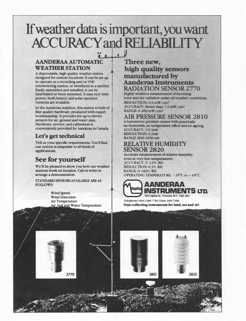
STANDARJ)SENS()RS AVAILABI.£ AIUi AS FOLLOWS:

Wind Speed Wind Direction Air Temperature

Water Temperature

THE USE OF SEA LEVEL TIDE GAUGE OBSERVATIONS IN GEODESY

Galo Carrera and Petr Van leek

Smvey Science University of Toronto Mississauga, Ontario

Canada L5L 1 C6

Survey ing Engineering Department University of New Brunswick Fredericton, New Brunswick

Canada E3B 5A3

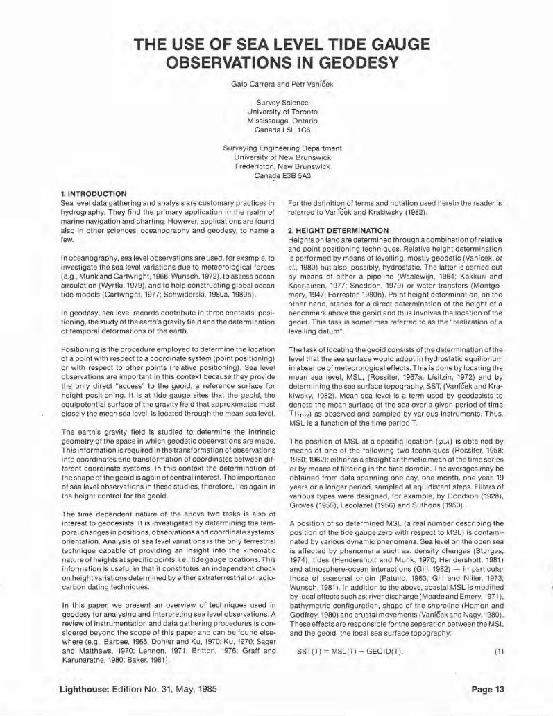
1. INTRODUCTION Sea level data gathering and analysis are customary practices in hydrography. They find the primary application in the realm of marine navigation and charting. However, applications are found also in other sciences, oceanography and geodesy, to name a few.

In oceanography, sea level observations are used, for example, to investigate the sea level variations due to meteorological forces (e.g., Munk and Cartwright, 1966; Wunsch, 1972), to assess ocean circulation (Wyrtki, 1979), and to help constructing global ocean tide models (Cartwright, 1977; Schwiderski, 1980a, 1980b).

In geodesy, sea level records contribute in three contexts: posi­tioning, the study of the earth's gravity field and the determination of temporal deformations of the earth .

Positioning is the procedure employed to determine the location of a point with respect to a coordinate system (point positioning) or with respect to other points (relative positioning). Sea level observations are important in this context because they provide the only di rect "access" to the geoid, a reference surface for height positioning. It is at tide gauge sites that the geoid, the equipotential surface of the gravity field that approximates most closely the mean sea level, is located through the mean sea level.

The earth's gravity f ield is studied to determine the intrinsic geometry of the space in which geodetic observations are made. This information is required in the transformation of observations into coordinates and transformation of coord inates between dif­ferent coordinate systems. In this context the determination of the shape of the geoid is again of central interest. The importance of sea level observations in these studies, therefore, lies again in the height control for the geoid.

The time dependent nature of the above two tasks is also of interest to geodesists. It is investigated by determining the tem­poral changes in positions, observations and coordinate systems' orientation. Analysis of sea level variations is the only terrestrial technique capable of providing an insight into the kinemat ic nature of heights at specific points, i.e., tide gauge locations. T his information is useful in that it constitutes an independent check on height variations determined by either extraterrestrial or radio­carbon dating techniques.

In this paper, we present an overview of techniques used in geodesy for analysing and interpreting sea level observat ions. A review of instrumentation and data gathering procedures is con­sidered beyond the scope of this paper and can be found else­where (e.g., Barbee, 1965; Dahler and Ku , 1970; Ku , 1970; Sager and Matthaws, 1970; Lennon, 1971; Britton, 1976; Graff and Karunaratne, 1980; Baker, 1981).

Lighthouse: Edition No. 31, May, 1985

For the defin ition of terms and notation used herein the reader is referred to Vanicek and Krakiw.sky (1982).

2. HEIGHT DETERMINATION Heights on land are determined through a combination of relative and point positioning techniques. Relative height determination is performed by means of levell ing, mostly geodetic (Vanicek, et a/., 1980) but also, possibly, hydrostatic. The latter is carried out by means of either a pipeline (Waalewijn, 1964; Kakkuri and Kii.ii.riii. inen, 1977; Sneddon, 1979) or water transfers (Montgo­mery, 1947; Forrester, 1980b). Point height determination , on the other hand, stands for a direct determination of the height of a benchmark above the geoid and thus involves the location of the geoid. This task is sometimes referred to as the " real ization of a levelling datum".

The task of locating the geoid consists of the determination of the level that the sea surface wou ld adopt in hydrostcttic equi librium in absence of meteorological effects. This is done by locating the mean sea level, MSL, (Rossiter, 1967a; Lisitzin, 1972) and by determining the sea surface topography, SST, (Vanfcek and Kra­kiwsky, 1982) . Mean sea level is a term used by geodesists to denote the mean surface of the sea over a given period of time T(t,,t2) as observed and sampled by various instruments. Thus, MSL is a function of the time period T.

The position of MSL at a specif ic location (<P ,A) is obtained by means of one of the following two techniques (Rossiter, 1958; 1960; 1962): either as a straight arithmetic mean of the time series or by means of filtering in the t ime domain. The averages may be obtained from data spanning one day, one month, one year, 19 years or a longer period, sampled at equidistant steps. Fi lters of various types were designed, for example, by Doodson (1928) , Groves (1955), Lecolazet (1956) and Suthons (1950) .

A position of so determined MSL (a real number describing the position of the tide gauge zero w ith respect to MSL) is contam i­nated by various dynamic phenomena. Sea level on the open sea is affected by phenomena such as: density changes (Sturges, 1974), tides (Hendershott and Munk, 1970; Hendershott, 1981) and atmosphere-ocean interact ions (Gill, 1982) - in part icular those of seasonal origin (Patullo, 1963; Gill and Niiler, 1973; Wunsch, 1981 ). In addition to the above, coastal MSL is mod ified by local effects such as: river discharge (Meade and Emery, 1971 ), bathymetric configurat ion, shape of the shorel ine (Hamon and Godfrey, 1980) and crustal movements (Vanfcek and Nagy, 1980). These effects are responsible for the separat ion between the MSL and the geoid, the local sea surface topog raphy:

SST(T ) = MSL(T)- GEOID(T). (1)

Page 13

Local SST differences may be measured directly using satellite altimetry (Marsh, 1983) or indirectly using steric levelling (Sturges, 1974; Forrester, 1980a). The SST may also be obtained from the permanent response of sea level to multiple forcing functions (wind stress, water temperature, barometric pressure, river discharge, etc.) Three methods are available to determine the frequency dependent response: the weighting function method (Munk and Cartwright, 1966; Cartwright, 1968) may be used in the time domain; cross spectral analysis (e.g., Wunsch , 1972; Garrett and Toulany, 1982; Palumbo and Mazzarella, 1982) and least squares response analysis (Steeves, 1981; Merry and Van leek, 1981; 1983) can be used in the frequency domain.

Figure 1 shows how the MSL and SST are employed in the determination of the height above the geoid of a geodetic refer­ence benchmark. A single connection of this type is enough to obtain levelled heights of many interconnected points (network). An example of a network that uses a single tide gauge is provided by the United European Levelling Net of 1955 (Rossiter, 1962a; Alberda, 1963).

Tide gauge connections can play an additional role in geodetic levelling networks by improving the accuracy of heights and height differences. The standard deviation , St:.H• of a height differ­ence, t.H, in geodetic levelling is dependent upon distance, L, and the standard deviation of a unit length, S 0 , (Vanicek and Grafarend, 1979), i.e.,

(2)

Therefore, the further a point is from the single geoid connection , the worse is the accuracy of its height above the geoid.ln order to curb such propagation of errors, multiple geoid connections are often used. It is of no surprise then to learn that multiple geoid connections were established in the past for the American (Berry,

1977; Whalen, 1980) and Canadian (Cannon, 1928; 1935; Lacha­pelle, eta/., 1977) levelling networks.

3. THE EARTH'S GRAVITY FIELD The determination of the earth's gravity field in geodesy is carried out by means of both extraterrestrial and terrestrial techniques. Extraterrestrial techniques include among others, the determina­tion of geoidal heights, N, from satellite derived geodetic heights, h, above a geocentric reference ellipsoid, and orthometric height, H" (Kouba, 1976; 1983; Vanfcek and John, 1983):

N = h- H0 . (3)

The above equation provides a natural accurate control of the geoid anywhere on land.

Terrestrial techniques include the solution of Stoke's and Vening­Meinez's problems (Moritz, 1980) for geoidal heights, N, and the deflections of the vertical,{, I], in which the data needed are the gravity anomalies which, in turn, are derived from the heights of the gravity observing stations: a gravity anomaly may be ex­pressed as

t.g = gobs + rHo- Yo• (4)

where goos is the observed gravity, r is a vertical gradient of gravity, H0 is the orthometric height of the station, and Yo is the corresponding normal gravity reckonned on a geocentric el­lipsoid.

Application of the law of propagation of random errors to equa­tions (3) and (4) gives

(5)

REFERENCE BENCH MARK

TIDE GAUGE

SEA SURFACE TOPOGRAPHY

Page 14

CONVENTIONAL ZERO ---------OF TIDE GAUGE

GEOID

LOCAL MEAN S.L.

INSTANTANEOUS

Lighthouse: Edition No. 31, May, 1985

•

and

(6)

where ITN, ITh and ITH:', are the standard deviations of the geoidal, geodetic and orthometric heights, and IT ~;9 and IT 90. , are the standard deviations of the gravity anomaly and the observed gravity. The value of ITH in equations (5) and (6) depends on the accuracy of geodetic levelling and, ultimately, once more on the accuracy with which the realization of the height datum is achieved at tide gauge sites.

Sea level information is needed also for various other purposes in extraterrestrial techniques. For example, in satellite altimetry, MSL and SST are required to calibrate the spacecraft radar (Mar­tin and Kolenkiewicz, 1981; Kolenkiewicz and Martin, 1982; Dia­mante, eta/., 1982). In the analysis of satellite orbital perturba­t ions it provides the reference surface from which initial heights for the tracking stations are reckonned (Schwarz, 1974).

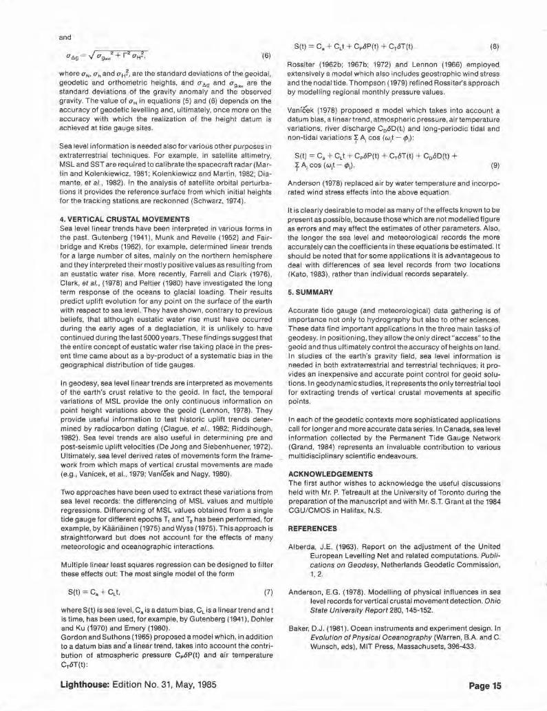
4. VERTICAL CRUSTAL MOVEMENTS Sea level linear trends have been interpreted in various forms in the past. Gutenberg (1941) , Munk and Revelle (1952) and Fai r­bridge and Krebs (1962) , fo r example, determined linear trends for a large number of sites, mainly on the northern hemisphere and they interpreted their mostly positive values as resulting from an eustatic water rise. More recently, Farrel l and Clark (1976), Clark, eta/., (1978) and Peltier (1980) have investigated the long term response of the oceans to glacial loading. Their results predict upl ift evo lution for any point on the surface of the earth with respect to sea level. They have shown, contrary to previous beliefs, that although eustatic water rise must have occurred during the early ages of a deglaciation, it is unlikely to have continued during the last 5000 years. These findings suggest that the entire concept of eustatic water rise taking place in the pres­ent time came about as a by-product of a systematic bias in the geograph ical distribution of tide gauges.

In geodesy, sea level linear trends are interpreted as movements of the ea rth's crust relative to the geoid. In fact, the temporal variations of MSL provide the only continuous information on point height variations above the geoid (Lennon, 1978). They provide useful information to test historic uplift trends deter­mined by radiocarbon dating (Clague, eta/., 1982; Riddihough , 1982). Sea level trends are also useful in determining pre and post-seismic uplift velocities (DeJong and Siebenhuener, 1972). Ultimately, sea level derived rates of movements form the frame­work from which maps of vertical crustal movements are made (e.g., Vanfcek, et al. , 1979; Vanfcek and Nagy, 1980).

Two approaches have been used to extract these variations from sea level records: the differencing of MSL values and multiple regressions. Differencing of MSL values obtained from a single tide gauge for different epochs T1 and T2 has been performed, for example, by Kaii.riii.inen (1975) and Wyss (1975). This approach is straightforward but does not account for the effects of many meteorologic and oceanographic interactions.

Multiple linear least squares regression can be designed to filter these effects out: The most single model of the form

S(t) = c. + CLt, (7)

where S(t) is sea level, c. is a datum bias, CL is a linear t rend and t is time, has been used, for example, by Gutenberg (1941}, Dahler and Ku (1970) and Emery (1980). Gordon and Suthons (1965) proposed a model which , in addition to a datum bias and' a linear trend, takes into account the contri­bution of atmospheric pressure Cp6P(t) and air temperature Cr6T(t) :

Lighthouse: Edition No. 31, May, 1985

(8)

Rossiter (1962b; 1967b; 1972) and Lennon (1966) employed extensively a model which also includes geostrophic wind stress and the nodal tide. Thompson (1979) refined Rossiter's approach by modelling regional monthly pressure values.

Vanfe'ek (1978) proposed a model which takes into account a datum bias, a linear trend , atmospheric pressure, air temperature variations, river discharge C0 6D(t;) and long-periodic tidal and non-tidal variations t Ai cos (wit - ¢ i):

S(t) =C.+ CLt + Cp6P(t) + Cr6T(t) + C0 6D(t) + t Ai cos (wit - ¢J (9)

Anderson (1978) replaced air by water temperature and incorpo­rated wind stress effects into the above equation .

It is clearly desirable to model as many of the effects known to be present as possible, because those which are not modelled figure as errors and may affect the estimates of other parameters. Also, the longer the sea level and meteorological records the more accurately can the coefficients in these equations be estimated. It should be noted that for some applications it is advantageous to deal with differences of sea level records from two locations (Kato, 1983}, rather than individual records separately.

5. SUMMARY

Accurate tide gauge (and meteorological) data gathering is of importance not only to hydrography but also to other sciences. These data find important applications in the three main tasks of geodesy. In positioning, they allow the only direct "access" to the geoid and thus ultimately control the accuracy of heights on land. In studies of the earth's gravity fie ld, sea level information is needed in both extraterrestrial and terrestrial techniques; it pro­vides an inexpensive and accurate point control for geoid solu­tions. In geodynamic studies, it represents the only terrestrial tool for extracting trends of vertical crustal movements at specific points.

In each of the geodetic contexts more sophisticated applications call for longer and more accurate data series. In Canada, sea level information collected by the Permanent Tide Gauge Network (Grand, 1984) represents an invaluable contribution to various multidiscipl inary scientific endeavours.

ACKNOWLEDGEMENTS The first author wishes to acknowledge the useful discussions held with Mr. P. Tetreault at the University of Toronto during the preparation of the manuscript and with Mr. S.T. Grant at the 1984 CGU/CMOS in Halifax, N.S.

REFERENCES

Alberda, J.E. (1963). Report on the adjustment of the United European Levell ing Net and related computations. Publi­cations on Geodesy, Netherlands Geodetic Commission , 1, 2.

Anderson, E.G. (1978). Modelling of physical influences in sea level records for vertical crustal movement detection. Ohio State University Report 280, 145-152.

Baker, D.J. (1981 ). Ocean instruments and experiment design. In Evolution of Physical Oceanography (Warren , B.A. and C. Wunsch, eds) , MIT Press, Massachusets, 396-433.

Page 15

1·

We build ARGO® systems to take a 110,000 volt lightning bolt and keep on sending accurate positioning data.

A lightning bolt flashes from the sky above the Mississippi Delta. An ARGO antenna takes

a direct hit - 110,000 volts surging down the antenna, across the spark gap system, through the surge coil and arrestor, to the blocking capacitor and transorbs.

Thanks to Cubic's ' 'overbuild' ' philosophy, the killing surge of power is reduced to 100 volts by the time it reaches ARGO's Range Processing Unit. Without interruption, ARGO continues transmitting to the survey ships offshore.

EVERY UNIT IS "TEST DRIVEN"

Lightning, extreme heat and cold, storms and a ccidents are facts of life in the offshore surveying environment. So we make sure every ARGO system is ready for the roughest duty before it leaves our labs . By

0 • • it :::: 0'

•••tl' .......

building each ARGO system, testing every component, and testing the entire system, again and again. Then subjecting each unit to extremes of temperature to test for thermal shock Finally, we "burn-in" each piece of equipment by operating it continuously for 30 days. Every single unit.

So, when you get your ARGO system, it 's already proved that it can take the toughest use. And, JUSt in case that's still not enough, redundancy is built in for critical input power connections. Nothing is left to chance.

ARGO: THE BEST KEEPS GETTING BETTER Since 1977, ARGO customers have had the best long range precision positioning system in the world. And we keep making it better. We've put over 50 design improvements into ARGO over the years. Whenever a customer sends us a unit for repair or reconditioning, it automatically goes through a design improvement retrofit cycle at no extra cost.

Cubic has a reputation to uphold, and every ARGO system sold proves it, time and time again. Precise position fixes you can depend on, and return to every time . At ranges averaging 300 to 400 nautical miles daytime and 150 to 200 at night . With up to 12 simultaneous range-range users. Selectable frequency control of up to 16 preset narrow bandwidth channels. Optional extended baseline software for ranging with up to 8 shore stations.

YOUR SOURCE FOR NAVIGATION AND POSITIONING SYSTEMS ARGO is just one of many precision products and systems we make to meet your navigation and positioning needs. Like ARGONAV, our new system that combines proven ARGO positioning ... ~4 performance with a powerful integrated navigation computer. And AUTOTAPE, the

T' microwave positioning ~ system that sets the standards for accuracy and dependability.

With over 30 years of experience and a 300 million dollar

corporation behind us, we offer you a Cubic solution to your positioning requirements.

For comprehensive literature call615/455-8524. Or write: Cubic Precision, P. 0. Box 821 TUllahoma, TN. 37388 . Telex (II): 810-375-3149.

r

Barbee, W.D. (1965). Tide gauges in the U.S. Coast and Geodetic Survey. In Proceedings on tidal instrumentation and pre­diction of tides, UNESCO, Paris.

Berry, R.M. (1977). History of levelling in the United States. Sur­veying and Mapping, 36, 2, 137-153.

Britton, R. Ed. (1976). Proceedings of the Symposium on Tide Recording. University of Southampton, U.K. Hydrographic Society Special Publication No. 4.

Cannon, J.B. (1928) . Adjustment of the precise level net of Can­ada. Geodetic Survey of Canada, Publication 28.

Cannon, J.B. (1935). Recent adjustments of the precise level net of Canada. Geodetic Survey of Canada, Publication 56.

Cartwright, D.E. (1968). A unified analysis of tides and surges round north and east Britain . Phil. Trans. R.S. London, A, 263, 1-55.

Cartwright, D.E. (1977). Oceanic Tides. Reports on Progress in Physics, 40, 665-708.

Clague, J., J.R. Harper, R.J. Hebda and D.E. Howes (1982). Late Quaternary levels and crustal movements, coastal British Columbia. Can. J. Earth Sci., 19, 597-618.

Clark, J.A., W.E. Farrell and W.R. Peltier (1978). Global changes in sea level: a numerical calculation. Quaternary Research , 9, 265-287.

De Jong, S.H. and H.F.W. Siebenhuener (1972). Seasonal and secular variations of sea level on the Pacific coast of Can­ada. Canadian Surveyor, 26, 1, 4-19.

Diamante, J.M. and B.C. Douglas, D.L. Porter and R.P. Masterson Jr. (1982). Tidal and geodetic observations for the SEASAT altimeter calibration experiment. J. Geophys. Res., 87, C5, 3199-3206.

Dohler, G.C. and L.F. Ku (1970). Presentation and assessment of tides and water level records for geophysical investiga­tions. Can. J. Earth Sci., 7, 607-625.

Doodson, A.T. (1928) . The analysis of tidal observations. Phil. Trans. R.S. London, A, 100, 305-329.

Emery, K.O. (1980). Relative sea levels from tide gauge records. Proc. Nat!. Acad. Sci. U.S.A., 77, 12, 6968-6972.

Fairbridge, R.W. and O.A. Krebs (1962). Sea-level and the south­ern oscillation. Geophys. J.R.A.S., 6, 532-545.

Farrell, W.E. and J.A. Clark (1976). On postglacial sea level. Geo­phys. J.R.A.S., 46, 647-667.

Forrester, W.D. (1980a). Principles of Oceanographic Levelling . In Proceedings of the Second International Symposium on ' Problems Related to the Redefinition of North American Vertical Geodetic Networks (G. Lachapelle, ed.), Canadian Institute of Surveying, Ottawa, 125-132.

Forrester, W.D. (1980b). Accuracy of water level transfers. In Pro­ceedings of the Second International Symposium on Prob­lems Related to the Redefinition of North American Verti­cal Geodetic Networks (G. Lachapelle, ed.), Canadian Institute of Surveying, Ottawa, 729-740.

Page 18

Garrett, Ch. and B. Toulany (1982). Sea level variability due to meteorological forcing in the northeast Gulf of St. Law­rence. J. Geophys. Res., 87, C3, 1968-1978.

Gill, A.E. (1982). Atmosphere-Ocean Dynamics. Academic Press, New York, 662 pp.

Gill, A. E. and P. Niiler (1973). The theory of seasonal variability in the ocean. Deep Sea Res., 20, 141-177.

Godin, G. (1972) . The Analysis of Tides. Toronto University Press, Toronto, 264 pp.

Gordon, D.L. and C.T. Suthons (1965). Mean sea level in the British Isles. Bull. Geod., 77, 205-213.

Graff, J. and A. Karunaratne (1980). Accurate reduction of sea level records. Int. Hydr. Rev., LVII, 2, 151-166.

Grant, S.T. (1984). The Permanent Tide Gauge Network in Can­ada. Annual Joint Meeting of the Canadian Geophysical Union and the Canadian Meteorologic and Oceanogra­phic Society, May 29 - June 1, Dalhousie University, Halifax, N.S.

Groves, G.W. (1955). Numerical filters for discrimination against tidal periodicities. Trans. Amer. Geophys. Un., 36, 6, 1073-1084.

Gutenberg, B. (1941 ). Changes in sea level, postglacial uplift, and mobility of the earth's interior. Bull. Geol. Soc. Amer. , 52, 721-772.

Hamon, B.V. and J.S. Godfrey (1980). Mean sea level and its interpretation. Marine Geodesy, 4, 4, 315-329.

Hendershott, M.C. (1981 ). Long waves and ocean tides. In Evolu­tion of Physical Oceanography (Warren B.A. and C. Wunsch, eds.), MIT Press, Massachusets, 292-341.

Hendershott, M.C. and W. Munk (1970). Tides. Ann. Rev. Fluid Dyn., 2, 205-224.

Kiiiiriiiinen, E. (1975). Land uplift in Finland on the basis of sea level recordings. Reports of the Finnish Geodetic Institute , No. 82.

Kakkuri, J . . and E. Kiiiiriiiinen (1977). The second levelling of Finland for the Aland Archipielago. Pub/. Finn. Geod. lnst. No. 82.

Kato, T. (1983). Secular and earthquake related vertical crustal movements in Japan as deduced from tidal records (1951-1981 ). Tectonophysics, 97, 183-200.

Kolenkiewicz, R. and Ch.F. Martin (1982). SEASAT altimeter height calibration. J. Geophys. Res., 87, C5, 3189-3197.

Kouba, J. (1976) . Doppler levelling . Canadian Surveyor, 30, 1, 21-31.

Kouba, J. (1983). A review of geodetic and geodynamic satellite Doppler positioning. Rev. Geophys. Sp. Phys., 21, 1, 27-40.

Ku, L.F (1970). The evaluation of the performance of water level recording instruments. In Proceedings on tidal instrumen­tation and prediction of tides, UNESCO, Paris, 167-180.

Lighthouse: Edition No. 31, May, 1985

Lachapelle, G., J.D. Boal, N.H. Frost and F.W Young (1977). Recommendations for the redefinition of the vertical refer­ence system in Canada. Collected Papers. Geodetic Sur­vey of Canada, 195-224.

Lecolazet, R. (1956). Application a !'analyse des observations de Ia maree gravimetrique de Ia methode de H. et Y. Labrouste dite par combinaisons Jineaires d'ordenees. Ann. Geoph., 12, 1, 59-71.

Lennon, G.W. (1966). An investigation of secular variation of sea level in European waters. Ann. Acad. Sci. Fennicae, A, Ill, 90, 225-236.

Lennon, G.W (1971 ). Sea level instrumentation, its limitations and the optimisation of the performance of conventional gauges in Great Britain. Int. Hydr. Rev. , XLVIII, 129-147.

Lennon, G.W. (1978). Sea level data and techniques for detecting vertical crustal movements. Ohio State University Report 280, 137-143.

Lisitzin, E. (1972). Mean sea level II. Oceanogr. Mar. Bioi. Ann. Rev., 10, 11-25.

Lisitzin, E. (1974) . Sea Level Changes. Elsevier, Amsterdam, 286 pp.

Marsh, J .G. (1983) . Satellite Altimetry. Rev. Geophys. Sp. Phys., 21, 3, 574-580.

Martin, C.F. and R. Kolenkiewicz (1981 ). Calibration validation for the GEOS 3 altimeter. J. Geophys. Res., 86, 87,6369-6381.

Meade, R.H. and K.O. Emery (1971 ). Sea level as affected by river runoff, Eastern United States. Science, 173, 425-428.

Merry, Ch. and P. Vanicek (1981 ). The zero frequency response of sea level to meteorological influences. University of New Brunswick Technical Report 82.

Merry, Ch. and P. Vanicek (1983). Investigations of local variations of sea surface topography. Marine Geodesy, 7, 1-4, 101-126.

Montgomery, R.H. (1947). Transfer of levels across water. Cana­dian Surveyor, IX, 5, 23-26.

Moritz, H. (1980). Advanced Physical Geodesy. Wichmann, Karls­ruhe, 500 pp.

Munk, W.H. and D. E. Cartwright (1966). Tidal spectroscopy and prediction. Phil. Trans. R.S. London, A, 259, 533-581.

Munk, W.H. and R. Revelle (1952). Sea level and the rotation ofthe earth. Ann. J. Sci. 250.

Palumbo, A. and A. Mazzarella (1982). Mean sea level variations and their practical appl ications. J. Geophys. Res., 87, C6, 4249-4256.

Patullo, J .G. (1963). Seasonal changes in sea level. In The Sea (M.N. Hill, ed.),lnterscience Publishers, New York, 485-496.

Peltier, W.R. (1980). Models of glacial isostacy and relative sea level. Dynamics of Plate Interiors, American Geophysical Union Geodynamic Series, 1, 111-128.

Riddihough, R.P. (1982). Contemporary movements and tecton­ics on Canada's west coast: a discussion. Tectonophysics, 86, 319-341.

Lighthouse: Edition No. 31, May, 1985

Rossiter, J.R. (1958) . Note on methods of determining monthly and annual values of mean water level. Int. Hydr. Rev., XXXV, 1, 105-115.

Rossiter, J.R. (1960). A further note on the determination of mean sea level. Int. Hydr. Rev., XXXVII, 2, 61-63.

Rossiter, J.R. (1962a). Report on the reduction of sea level obser­vations (1940-1958) for R.E.U.N. Trav. Ass. Int. Geod., 21, 159-184.

Rossiter, J.R. (1962b). Long term variations in sea level. In The Sea (M.N. Hill, ed.), lnterscience Publishers, New York, 590-610.

Rossiter, J.R. (1967a). Mean sea level. In International Dictionary of Geophysics (S.K. Runcorn, ed.), Pergamon Press, Oxford, 2, 929-934.

Rossiter, J.R. (1 967b). An analysis of annual sea level variat ions in European waters. Geophys. J.R.A.S., 12, 259-299.

Rossiter, J.R. (1972) . Sea level observations and their secular variation. Phil. Trans. R.S. London, A, 272, 131 -139.

Sager, G. and N. Matthaws (1970) . Theoretical and experimental investigations into the damping properties of tide gauges. In Report on the Symposium of Coastal Geodesy (R. Sigl, ed .), Munich, 201-218.

Schwarz, K.P. (1974) . Tesseral harmonic coefficients and station coordinates from satelite observations by col location. Ohio State University Report 217.

Schwiderski , E.W. (1980a). On charting global ocean tides. Rev. Geophys. Sp. Phys. , 18, 1, 243-268.

Schwiderski, E.W. (1980b). Ocean tides, Part II : A hydrodynamical interpolation model. Marine Geodesy, 3, 219-255.

Sneddon, J. (1979). The wider application of hydrostatic levelling. Survey Review, XXV, 191, 23-27.

Steeves, R.R. (1981 ). Estimation of gravity tilt response to atmos­pheric phenomena at the Fredericton tiltmetric station using a least squares response method. University of New Brunswick Technical Report 79.

Suthons, C. (1950) . The Admiralty semi-graphic method of har­monic tidal analysis. Admiralty Tidal Handbook No. 1.

Sturges, W (1974). Sea level slope along continental boundaries. J. Geophys. Res., 79, 6, 825-830.

Thompson, K.R. (1979). Regression models for monthly mean sea level. Marine Geodesy, 2, 3, 269-290.

Van leek, P. (1978). To the problem of noise reduction in sea level records used in vertical crustal movement detection. Phys. Earth Planet. Int., 17, 265-280.

Van leek, P. and E.W. Grafarend (1979). On the weight estimation in leveling. NOAA Tech. Rep. NOS 86 NGS 17.

Vanlcek, P. and S. John (1983). Evolution of geoid solutions in Canada using different kinds of data. Proceedings of the International Association of Geodesy Symposia, Ham­burg, 1, 609-624.

Page 19

Vanlcek, P. and E. Krakiwsky (1982). Geodesy: The Concepts. North Holland, Amsterdam, 691 pp.

Vanltek, P. and D. Nagy (1980). Report on the compilation of the map of vertical crustal movements in Canada. Earth Phys­ics Branch, EMR, Open File 80-2.

Vanltek, P., R.O. Castle and E. Balazs (1980). Geodetic levelling and its applications. Rev. Geophys. Sp. Phys., 18, 2, 505-524.

Van leek, P., M.R. Elliott and R.O. Castle (1979). Four dimensional modelling of recent vertical movements in the area of the southern California uplift. Tectonophysics, 52, 1-4,287-300.

Waalewijn, A. (1964). Hydrostatic levelling in the Netherlands. Survey Review, XVII, 131,212-271.

Whalen, Ch. (1980). Status of the national geodetic vertical con­trol network. In Proceedings of the Second International Symposium on Problems Related to the Redefinition of North American Vertical Geodetic Networks (G. Lacha­pelle, ed.), Canadian Institute of Surveying, Ottawa, 11 -24.

Wunsch, C. (1972). Bermuda sea level in relation to tides, weather, and baroclinic f luctuations. Rev. Geophys. Sp. Phys., 10, 1-49.

Wunsch, C. (1981 ). Low freqency variabil ity of the sea. In Evolu­tion of Physical Oceanography (Warren B.A. and C. Wunsch, eds.), MIT Press, Massachusets, 342-374.

Wyrtki , K. (1979). Sea level variations: Monitoring the breath of the Pacific. EOS, 60, 30, 25-27.

Wyss, M. (1975) . Mean sea level before and after some great strike-slip earthquakes. Pure and Applied Geophysics, 113, 107-118.

THE HYDROGRAPHIC CONTOURING SYSTEM PRACTICAL EXPERIENCES

By Dan MacDonald

Kal Czotter

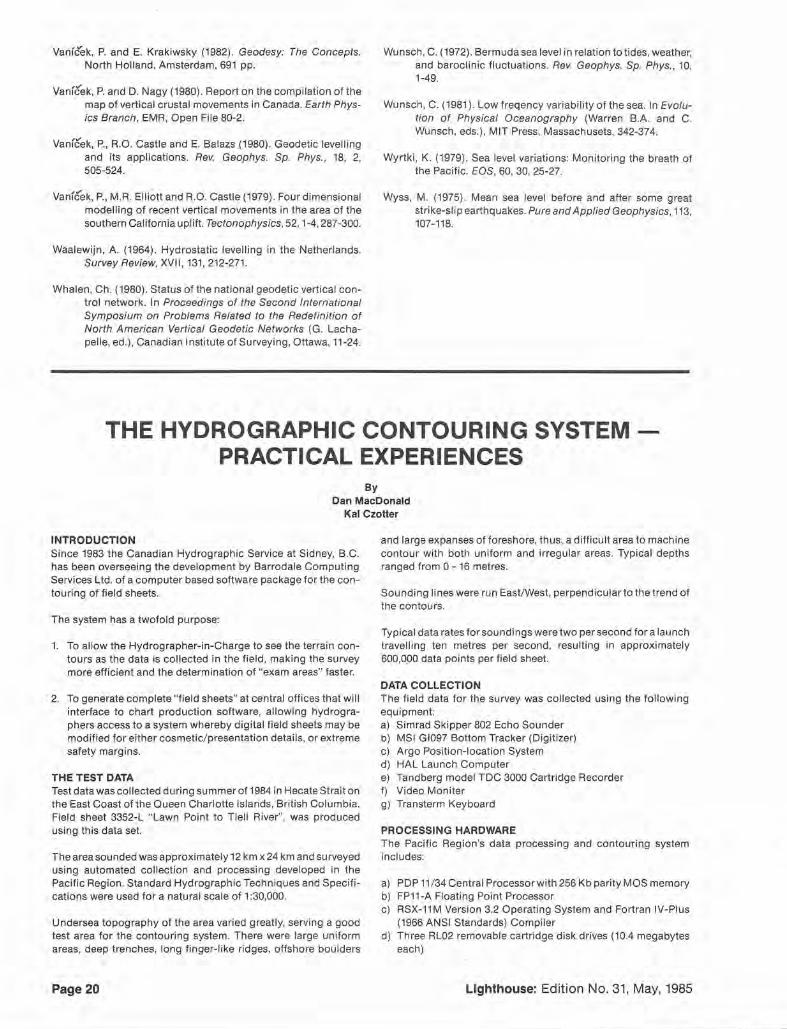
INTRODUCTION Since 1983 the Canadian Hydrographic Service at Sidney, B.C. has been overseeing the development by Barrodale Computing Services Ltd. of a computer based software package for the con­touring of field sheets.

The system has a twofold purpose:

1. To al low the Hydrographer-in-Charge to see the terrain con­tours as the data is collected in the field, making the survey more efficient and the determination of "exam areas" faster.

2. To generate complete "field sheets" at central offices that will interface to chart production software, allowing hydrogra­phers access to a system whereby digital fie ld sheets may be modified for either cosmetic/presentation details, or extreme safety margins.

THE TEST DATA Test data was collected during summer of 1984 in Hecate Strait on the East Coast of the Queen Charlotte Islands, British Columbia. Field sheet 3352-L "Lawn Point to Tlell River", was produced using this data set.

The area sounded was approximately 12 km x 24 km and surveyed using automated col lection and processing developed in the Pacific Region. Standard Hydrographic Techniques and Specifi­cations were used for a natural scale of 1 :30,000.

Undersea topography of the area varied greatly, serving a good test area for the contouring system. There were large uniform areas, deep trenches, long finger-like ridges, offshore boulders

Page 20

and large expanses of foreshore, thus, a difficult area to mach ine contour with both uniform and irregular areas. Typical depths ranged from 0 - 16 metres.

Sounding lines were run East/West, perpendicular to the trend of the contours.

Typical data rates for soundings were two per second for a launch travelling ten metres per second, resu lting in approximately 600,0_00 data points per field sheet.

DATA COLLECTION The field data for the survey was collected using the following equipment: a) Simrad Skipper 802 Echo Sounder b) MSI GI097 Bottom Tracker (Digitizer) c) Argo Position-location System d) HAL Launch Computer e) Tandberg model TDC 3000 Cartridge Recorder f) Video Moniter g) Transterm Keyboard

PROCESSING HARDWARE The Pacific Region 's data processing and contouring system includes:

a) PDP 11/34 Central Processor with 256 Kb parity MOS memory b) FP11 -A Floating Point Processor c) RSX-11 M Version 3.2 Operating System and Fortran IV-Pius

(1966 ANSI Standards) Compiler d) Three RL02 removable cartridge disk drives (10.4 megabytes

each)

Lighthouse: Edition No. 31 , May, 1985

•

Drive 0 Operating System software and user files Drive 1 Contouring System (Task images, parameter files) Drive 2 Data Disk

e) Two Kennedy Model 9000 Magnetic tape drives (1600 bpi)

f) Tandberg Model TDC 3000 Cartridge Re-corder

g) Calcomp Model1038 Drum Plotter h) Tektronix 4014 Graphics Terminal i) VT100 Display Terminals j) DECwriter Ill Printing Terminals

PROCESSING

BRITISH

COLU('IBIA

COLOMBIE

BRITANNIOUE I

After the hydrographer has completed his shift in the launch, data processing begins.

1) Data recorded on cartridge is.first archived onto 9-track magnetic tapes- one file per launch per shift.

suRvEY 1· i

2) Each file is processed off the 9-track archived tapes as a quality check on archiving.

3) Each file is processed using HALPRO- a program which checks input syntax, posi­tion computation and interpolation, posi­tion, depth and output time.

4) Depths are cleaned with ZCLEAN- a pro­gram which generates a graph ic represen­tation of depth data giving a good check as to depth quality against the actual sound­ing roll. ZCLEAN has options to remove and smooth depths resulting in a smooth single line representation of the bottom.

AREA

1 Js·

5) Once the bottom is portrayed precisely, tide corrections are applied to each file using the program ATIDES.

CONTOURING As each file is processed it is written onto magnetic tape in Filesll formats. This is done to save disk space. The contouring program will read the data sequentially and so as long as the files are put onto tape in the order that they are requested, then no time will be wasted in slow tape searches.

Once all the data for an area has been processed (i.e. all files with sounding lines through the area), then that area may be con­toured. The user runs a program that allows him to interactively setup the contouring system's runtime parameters. Once set, the contouring system is initiated. ·

The contouring program is run in "Batch" mode, meaning once started, it runs until either it completes the job, or (heaven forbid) it crashes. The user defined runtime parameters control the sys­tem, telling it not only what input data sets to use, but also how to process the data (i.e. the area of interest, line spacing estimates, grid mesh size, required contours, etc.). The entire batch job consists of many stages, some of which may or may not be present depending upon the runtime parameters set.

1) Line Numbering The first step is to number the sounding lines. This data can be either PARALLEL or NON-PARALLEL. NON-PARALLEL line data is data whose lines overlap extensively. Lines are broken by gaps in the data that exceed a user-defined length. PARALLEL line data is data whose lines don't overlap (i.e. no exam, non check-lines). Parallel lines are broken by gaps or reversals in direction.

Lighthouse: Edition No. 31, May, 1985

While advantages can be taken of parallel data's layout, in prac­tice very little of the data collected so far is truly parallel. As long as the data contains overlapping sounding lines, clover- leafed exams, and perpendicular check lines, then the data is essentially non-parallel.

Output from this phase is a GPCBASE sequential fi le, in Hydro­graphic Contouring System (HCS) format.

2) Point Flagging Data points corresponding to either local deeps or shoals are marked as such. The term " local" is defined by two parameters: rise height and run length.

POINT FLAGG!~

shoal •• T- -- -- -- ~..__ -- --... , • RISE • saoal HEIGHT • L +- --•-- . I. •I

.- -+- ---. RISE s~fal ., I , ... ~ t• HEIGHTe .• •e e , •• e ~ _I xee~ I ~.•!__ _ -;:,P dee_l_

I I I I t-- MAXIMUM I RUN LENGTH -1 I I I I l--- LOCAl~ LOCAL I LOCAL jLOCALtLOCAL !LOCAL I

Page 21

1

•

Each of the local areas is marked. The first local is such because it exceeds the run length. The others are locals because the bottom crosses the rise heights.

Contour intercepts are also determined in this phase. If no actual data point exists at the contour intercept, then the value is interpo­lated from neighbouring points. In some cases, determination of line numbers is crucial to this interpolation (i .e. selected soundings).

Output from this phase is another GPCBASE file. This file may be "weeded" leaving only significant points- shoals, intercepts and endpoints of lines. Weeding compresses the data file size.

3) Gridding The general technique in gridding is to overlay a rectangular grid mesh on the area to be contoured. Points are read in the closest grid nodes are determined by interpolation between data po ints to find where the contour line would pass. Once all the points have been read, the neighbouring grid nodes are "scanned" and those nodes not already set are computed. A third smoothing phase is optional.

Two methods of gridding are available: one is for parallel data, the other for non-parallel data. Grids may be merged so that one grid can be generated from parallel data, another from non-parallel data and the two combined into one. Unfortunately this doubles the processing time required to produce the final grid as the two streams of data must be processed separately to create two grids. Additionally, each grid will be produced from its data only, and does not have access to the other information for that area. The grids are then combined in a strict OR : if the first grid value is valid, use it, elsE) if the second is valid use it, else the point is not defined. Note that the grid is not further smoothed after the combination and discontinuous boundaries may arise if there exists a depth error between the two.

4) Linking Grid to Data After the grid has been produced, the actual data points (i.e. shoals, deeps and intercepts) must be linked to it. This is achieved via the grid pointer file (GRDPNTR).

The GRDPNTR file has the same format as the grid file, except that instead of nodes representing depths, each node indexes directly into the contour intercept (CNTINTC) file, pointing to the first data record for that grid mesh cell. In addition to storing shoals, deeps, intercepts (and points if included), the CNTINTC file also contains interpolated values marking where the data line leaves each grid mesh cell.

5) Contouring Three types of contouring are available:

i) from grid only. Contours are generated by fitting a curve through nodes in the grid. This is the fastest gridding option .

ii) from grid using CNTINTC and GRDPNTR files. Contours are first generated from grid, and then modified by the data in the CNTINTC file.

iii) respecting intercepts. Contours are generated as in ii) above, but the contours are modified so that they run through the marked contour intercept.

The three contouring methods produce charts that are very sim­ilar; the first two are almost identical. Contouring respecting intercepts results in tiny ticks along the lines where soundings were run . Other than these ticks, the chart is identical to that

Page 22

produced using the CNTINTC file without respecting intercepts.

While contour intercepts may seem like a good idea, they are difficult to justify mathematically. In one direction (along the data line) accuracy is enforced to less than one metre, while between lines there are 150 metre gaps. Contouring respecting intercepts does not appear to be a good contouring scheme.

6) Highs and Lows Two stages of terrain extrema may be produced. The first phase involves determining a shoal or a deep value for each closed contour, if such a data point exists in the CNTINTC file. The second optional phase fills the entire chart with the shoalest data in the area. This density can be approximately controlled.

7) NTX Interface The final stage is to take the various plot files containing the contours and the highs and lows and convert them to NTX format, for interfacing with the Graphical On-Line Manipulation and Dis­play System (GO MADS). Output from this final phase is an NTX tape.

PROBLEMS The contouring package was run during the fall of 1984 on the data collected that summer. Several problems became apparent, the greatest of which were caused by the volume of data. The original idea was to run the package using "raw" data (vs. selected soundings) so that the greatest amount of information would be used to generate the contours. A single field sheet at 1:30,000, covering an area of 12 km x 24 km field sheet could be contoured from the grid . If the data is not weeded then only about one thirtieth of the field sheet may be processed at one time.

Using selected sounding instead of raw data, the entire field sheet may by contoured from the grid. If highs and lows are required (so that the CNTICTC file must be constructed) then only about half the field sheet may be processed on a run.

There are two major factors for these limiting constraints:

1) GPCBASE file sizes.

Each GPCBASE contains data points after they have been line numbered, and later after having shoals, deeps and intercepts marked. While these files are in binary format to minimize space, processing requires that at least two of them exist at one point in the processing. Very soon the RL02's capacity is exceeded.

2) CNTINTC record index. The CNTINTC file is the worst bottleneck . It contains each data record (from GPCBASE) plus some additional points (where the line leaves the grid mesh cell), each of which is directly addressed by a record number index. Due to memory constra ints, this record index variable is an INTEGER*2, meaning it cannot take on a value greater than 32,767. Obviously, the 600,000 data points alone exceed this limit.

Additionally, the PDP 11 's 64K memory constraint has influenced the development of the contouring systems, in many ways to the systems' detriment. An example is a problem that had arisen in the extreme determination routine because of array size dimen­sions (which cannot be increased due to the computer's small memory.)

One other difficulty with the HCS relates to processing time. To process one field sheet using raw data and highs and lows required approximately 24 hours computing time to generate the field sheet. On the other hand, contouring the entire area from selected soundings only (the same information used to contour a

Lighthouse: Edition No. 31, May, 1985

surface towed subbottom profiler.

H untec's Hydrosonde SeaOtter is a new high resolution

marine seismic profiling system providing a high intensity acous-tic pulse with wide frequency bandwidth: and SeaOtter is priced as much as 50% below com par-able system capabilities.

SeaOtter can be supplied:

(a) as a complete sound source with power/ energy storage units (b) as a catamaran mounted sound source compatible with your power/tow cables (c) as a replacement trans-ducer to your existing towed vehicles.

The heart of the SeaOtter is a new compact boomer accepting inputs of 50 through 1000 joules per shot at two shots per second (2000 watts); producing a high intensity acoustic pulse; a wide frequency bandwidth for superior resolution and subbottom penetrations up to 100 metres. A unique acoustic filter el iminates

Huntec Hydrosonde

It's modular cost effective & affordable

sea surface reflections, reduces secondary oscillations and bubble pulse effects. Modular & versatile.

The SeaOtter is small, compact, lightweight and p.owerful.

It's ready for use w ith most energy/power sources. No special handling equipment required, the rugged assembly can be operated from small survey craft, its pigtai I connections compatible with various power sources or with Huntec's Power Control Unit/ Energy Storage Un it combination.

SeaOtter features: •

• Compact and light in weight for ease of handling and transportation.

• Modular construction for flexibility.

• Input energies to 1000 jou les per shot.

• Directional sound source at high frequencies- no back radiation or surface ghosting.

• Pulse repetition rates to 10 per second - maximum average power 2000 watts.

• No bubble pulse or secondary oscillation.

• Wide acoustic bandwidth for high resolution and excellent penetration.

• High energy content at low frequencies for penetration .

If you are interested in learning how SeaOtter can improve your profiling efficiency and reduce your survey costs dramatically, contact:

HUNTEC GEOPHYSICS

I ., 1750 Brimley Road, Scarborough Ontario, Canada M1P 4X7 Phone: (416) 299-4100 Telex: 06-963640

t

•

sheet by hand) takes about 70 minutes.

These time problems are re lated to the storage and CNTINTC problems mentioned above. Re-running the program is itself a time-consuming problem. Rereading the data files from magnetic tape rapidly exaggerates the time taken for processing. Of the 24 hours taken to process the thirty sub-sheets, approximately 40% was time required to repeatedly read in data.

ADVANTAGES What are the advantages of such a computer based contouring system? There are the obvious ones of speed and consistency. Computers are best at processing vast amounts of information quickly and consistently (if supplied with the proper resources).

The advantages of a digitally based contouring system are in its flexibility. The stored digital grid is easily accessed to generate various displays both on graphics screen and paper plot. Charts of different scales may be produced from the same grid, thus assuring complete consistency (accuracy depends upon the grid chosen for the survey).

If used properly in the field the HCS can increase the efficiency of the survey. If the data can be collected in blocks, then small areas

can be processed and contoured whle the survey party is still in the area, giving them a graphic representation of the bottom, thus making the choice of examinations and split lines more apparent and faster.

SUGGESTED IMPROVEMENTS If full advantage is to be made of parallel data, then the soundings must be collected in parallel lines. Perpendicular check lines should not be included with contouring data. Rather, these lines could be plotted out as soundings that lay over the contours as a check.

Exam format should be re-evaluated. Instead of clover-leafed patterns, a dense series of parallel lines would cover the ·area much more thoroughly.

Further improvements are needed. Some sort of file management system will be required to keep data files organized (and opera­tors sane). Colour graphics would greatly aid data file recognition for track plots, etc.

Work is presently underway to create a VAX version of the HCS system. A 32-bit machine such as VAX, when coupled with larger disk drives, will make the field system viable.

NEXT GENERATION PLOTTERS A study of Raster, Electostatic

and Pen type plotters

Don H. Vachon Canadian Hydrographic Service

Ottawa, Ontario.

1.0 Introduction This article investigates various plotting technologies, i.e., those technologies which showed the most potential for our next gen­eration charting requirements. Items examined were cost, speci­fications and possible applications. The types of plotters re­viewed were raster, electrostatic and multi-pen. The research was limited to these plotters since preliminary analysis concluded that this grouping best met the criteria for verification and/ or "final product" plotting for marine cartography.

1.1 Introduction to raster plotters With increased automation and the growing demand for preci­sion, quality and speed, more and more applications are moving towards raster technology for hardcopy output. Historically, pre­cision applications have been primarily provided by the electro­mechanical aperture photoplotters produced by companies such as Gerber Scientific Instrument Company and Konsberg North America Inc. However, with the high line densities found in nauti­cal charts, the times required for photoplotting have been very long. Also, the complexity of these vector photoplotters "can" lead to a poor MRBF (mean-time-before-failure), whereas the relative simplicity of most raster architectures (drum type) pro­vide a very good MTBF. Section 2.0 contains a research brief on available raster type plotters.

1.2 Introduction to electrostatic plotters Electrostatic plotters produce color or monochrome plots by selectively creating minute electrostatic dots on paper or film. A

Page 24

permanent image is then produced by depositing liquid toner on the charged areas. Multiple passes are used to produce a color image. The first pass assures proper reg istration, the following 4 passes writes in one of four toning colors. Registration is main­tained by high precision tracking.

Pen and/or photo plotters slow to a crawl when vector count increases substantially. Though the electrostatic plotter requi res additional processing time (vector to raster conversion) , the actual plotting speed remains unaffected. Shading and/ or color fill adds dimension and meaning to charts. This feature is slow and limited with pen plotters and impractical with photo-plotters. In the electrostatic environment, color shading is added without loss of any plotting speed. Section 3.0 examines the electrostatic plotters presently available.

1.3 Introduction to multi-pen plotters Pen plotters are presently used to provide fast and accurate verification plots at a comparatively low cost. With the need for color (color chart processing), selection of a multi-pen, intelligent plotter was indicated. This plotting technology has evolved and matured through the years; therefore, the determining factors were cost, ease of integration with present application software, functionality, bundled software routines, accuracy and service. Section 4.0 reviews some of the major multi-pen plotters on the market today.

Lighthouse: Edition No. 31, May, 1985

•

Table 1.0 Plotters - General information

Type Resolution Speed Comments

Raster very fast - can be used to produce veri-good fication plots

-generates reproduction nega-tives (including color separation plots) - requires photo-mechanical processing

Electro- good very -verification or direct final pro-static fast duct generation (paper chart)

- can also generate reproduc-tion negatives and positives (inclu-ding color separation plots) - photo-mechanical processing not required

Multi - good slow - Color verificat ion plots possi-pen ble (8 pens= 8 colors)

- color fill emulated by cross-hatching

2.0 Raster Plotters Present photo-plotters (not raster) use optical heads, which write on film with light. Due to the complexity of these optical heads (lens system, symbol disk, mechanical control mechanisms, etc.) they are expensive and not readily serviceable in the field. The photoplotters, though giving excellent line and symbol quality, are slow and very complex. There is also a limit on the number of symbols that can by used (e.g., 96), therefore data must be separ­ated according to the symbol disk in use and the symbol disk must be changed under dark room conditions.

Extensively used in the graphics art industry is the raster-drum plotter, which now operates at approximately 2000 lines per inch. This resolution gives a high-quality image, good for most map­ping applications. The quality of the output is directly related to the vector to raster conversion software, and much work has recently been done towards generating economic and high­quality results. The greatest advantages of raster plotters are their unlimited symbology and drawing speed (for the larger and more complex charts).

There are four alternative architectures in use for raster data plotting. They are:

1) Externa l drum 2) Relay lens/field-flattener lens 3) X-Y mechanical scanner 4) Internal curved-surface scanner

The external drum configuration is the basis for both the Optron­ics and Scitex plotters (Figure 1 ). The main advantage of this architecture is its inherent simplicity. The mechanical tolerances of the motion devices provide the only limits to the high geometric accuracy and repeatabili ty. Potential error can arise during the actual loading of the film media (film buckling). However, with proper operator training these errors can be minimized, and acceptable images can be generated. Generally, the external drum architect ure is primarily used in applications requiring high resolut ion and large image formats such as cartographic plotting.

Lighthouse: Edition No. 31, May, 1985

Figure 1: External Drum Plotter (after NIMS, 1984)

The relay lens/field-flattener lens architecture directs focused, modulated light across the fieJd of a lens in a raster fashion (stationary fi lm: Figure 2) and repetitively over the same line across moving media (Figure 3) producing an image. Due to the extremely ti ght tolerances required for both the lens and CRT, geometric accuracy becomes diff icult to obtain. Also, the aging characteristics of the CRT make it difficult to consistently re­create tonal shades. The relay lens can be very intricate and costly when high performance is required (high resolution and good color registration) .

Figure 2 Relay Lens (after NIMS, 1984)

Figure 3 Relay Lens (after NIMS, 1984)

Page 25

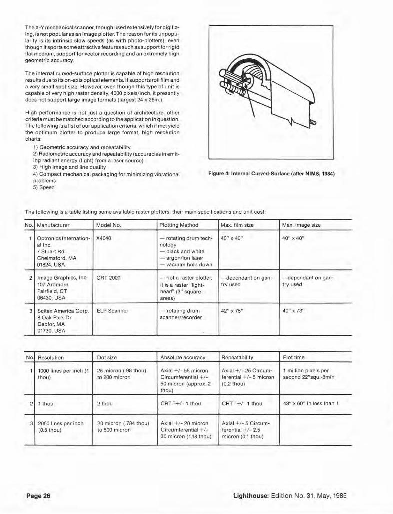
The X-Y mechanical scanner, though used extensively for digitiz­ing, is not popular as an image plotter. The reason for its unpopu­larity is its intrinsic slow speeds (as with photo-plotters), even though it sports some attractive features such as support for rigid flat medium, support for vector recording and an extremely high geometric accuracy.

The internal curved-surface plotter is capable of high resolution results due to its on-axis optical elements. It supports ro ll fi lm and a very small spot size. However, even though this type of unit is capable of very high raster density, 4000 pixels/inch, it presently does not support large image formats (largest 24 x 26in.).

High performance is not just a question of architecture; other criteria must be matched according to the application in question. The following is a list of our application criteria, which if met yield the optimum plotter to produce large format, high reso lution charts:

1) Geometric accuracy and repeatability 2) Radiometric accuracy and repeatabi lity (accuracies in emit­ing radiant energy (light) from a laser source) 3) High image and line quality 4) Compact mechanical packag ing for minimizing vibrational problems

Figure 4: Internal Curved-Surface (after NIMS, 1984)

5) Speed

The fo llowing is a table listing some available raster plotters, th~ ir main specifications and unit cost:

No. Manufacturer Model No. Plotting Method Max. film size Max. image size

1 Optronics I nternation- X4040 -rotating drum tech- 40" X 40" 40" X 40" al ine. nology 7 Stuart Rd. - black and white Chelmsford, MA - argon/ ion laser 01824, USA -vacuum hold down

2 Image Graphics, Inc. CRT 2000 - not a raster plotter, - dependant on gan- - dependant on gan-107 Ardmore it is a raster " light- try used t ry used Fairfield, CT head" (3" square 06430, USA areas)

3 Scitex America Corp. ELP Scanner - rotating drum 42" X 75" 40" X 73" 8 Oak Park Dr scanner/ recorder Debfor, MA 01730, USA

No Resolution Dot size Absolute accuracy Repeatabi lity Plot time

1 1000 lines per inch (1 25 micron (.98 thou) Axial +1- 55 micron Axial + ! - 25 Circum- 1 million pixels per thou) to 200 micron Circumferential +1- ferential +I- 5 micron second 22"squ.-8min

50 micron (approx. 2 (0.2 thou) thou)

2 1 thou 2thou CRT ::.+/- 1 thou CRT ::.+/- 1 thou 48" x 60" in less than 1

3 2000 lines per inch 20 micron (.784 thou) Axial +!- 20 micron Axial +1- 5 Circum-(0.5 thou) to 500 micron Circumferential +1- ferential +!- 2.5

30 micron (1 .18 thou) micron (0.1 thou)

Page 26 Lighthouse: Edition No. 31, May, 1985

No .. Cost Warranty Service

1 Scanner/ Recoder $263,000.00 12 months/3 months labor Warranty extension: 12 months/12 Recorder: $225,000.00 installation: 2 man/week months. 1/ 0 interface $9,350.00 run length 1st day charge $1,919.00 1% of cost per month of extension

encoder/decoder $9,350.00 subsequent days $704.00 PM program: $4,800/yr 3 visits, 10% registration $3,500.00

** $247,200.00 **

2 CRT head $165,000 (US) SVG 300 $ 35,000 (US) software $ 2,500 (US) Gerber gantry $215,000 (US)

$417,000 (US)

3 note: ELP scanner hardware is same as R280's

price without continuous tone option: $275,000.00 (US)

price with continuous tone option: . $300,000.00 (US)

Image Graphics 2000 Item 2, the Image Graphics 2000, is a high-speed, large format flatbed photocomposition system which replaces the standard optical photohead with a computer-controlled cathode ray tube exposure head. Plotting times have been decreased in the order of 20 to 200 times at several of the existing sites. The actual number varied according to the format and content of the data in question. A typical large format chart (36" x48") can be plotted in 25 minutes or less. Graphics arts quality can be obtained for the formation and placement of nomenclature data and feature sym­bology. A variety of font styles and sizes are possible, as well as a 1 degree step symbol rotation . The photocomposition format can be prepares directly on a host computer or alternatively via one of the furnished format conversion packages. These software pack­ages enable a user's standard plotting format to be converted to the photocomposition format in real-time. The software provided runs under the RSX11 M operation system. Though this option offers some attractive features, it additionally suffers some innate drawbacks. Since the exposure device is a CRT, it becomes diffi­cult to achieve geometric accuracy due to the extremely stringent tolerances required. In addition, the CRT's analog technology and the aging attributes of the phosphor make it very difficult to maintain consistent tonal quality. Finally, the cost of this option is comparatively high since an X-Y plotting gantry (i.e., Gerber) is also necessary.

Optronics Photomation X4040 Item 1, the Optronics photomation 4040 scanner/laser film recorder, offers dual mode capabilities, that is, it operates both as an input digitizing scanner and as a output laser plotter. Although input by way of document scanning is not examined in this article, the reader is encouraged to read the sub-section titled "E>lgitizing Scanner" , for an introduction to the topic. This particular model is restricted to an image format size of 40" x 40" , which is less than our required standard chart size of 36" x 48" . Although this problem could be bypassed by mosaicing adjacent chart sec­tions, the error introduced by such a process is undesirable. Another disadvantage lies in its conversion software, which is still in its infancy and is not very user fr iendly (Summer/84).

Lighthouse: Edition No. 31, May, 1985

discount on rep lacement parts dis-count on 1st/2nd day service charge

9% of cost per annum .. . 24 hours ser-vice 3 field engineers in Montreal and Toronto Future local field service planned (Ottawa)

Scitex ELP Scanner The Scitex ELP Scanner (item 3) offers high resolution and for­mat handling capabilities. Hundreds of ILPs are in use today with applications ranging from publications to PC boards. The ILP offers dual mode capabilities, that is, output plotting as well as input scanning via a field upgrade kit. In the raster plotting mode the device utilizes a laser to expose photosensitive media mounted on a rotating drum. This option is comprised of the plotter, control electronics, an HP1000-E CPU, a 300 Mbyte Win­chester mass storage disk, a CDC 800/1600 magtape drive and an alphanumeric CRT terminal. This system can also generate tone plots which emu late screens and plate ready negs at a 2000 lines per inch resolution. The plotting media consists of high-contrast orthochromatic film or paper, continuous tone f ilm (with variable density exposure option) or lith film. The drum is equipped with a row of 15 registration pins, and an optional registration punch is available to fac ilitate use of the pins (straightness tolerance for pins and punch is +/- 0.0004"). Variable-density exposure is provided through an optional electronics kit and software driver ($25,000 U.S.). This kit controls laser modulation, providing up to 256 intensity levels; resolution, however, becomes limited to the 200-1000 lines per inch range. The input scanner can handle image sizes up to 40" x 73", while detecting up to 641evels of gray (16 different shades can be stored). The input hardware automat­ically packs the scanned data into a simple, compact format (run-length encoding) before transferring it to mass storage.

The samples examined (Figure 6) at the 2000 lines/inch resolu­tion showed very good contrast and line densities, even at a 0.002" line weight. "Jaggies"* were detected, by way of micro­scopes, on the diagonals. The worst case deviation of +I- 0.0005" is directly related to the matrix of individually addressed points or dots, where the dot size at 2000 lines/inch is 0.0005". Line enhancement techn iques might filter out said jaggies, an option stil l under investigation.

* "Jaggies" is a commonly used term meaning steps in drawn lines, such as staircasing on diagonals:

Page 27

•

One installation, namely U.S. Geological Survey (USGS), had been using a Kongsberg plotter with a Barr and Stroud light head. They have since upgraded to the ELP scanner and are success­fully plotting from their existing Konsberg plot tape library. They have accomplished this by way of a Gerber Translator which with minimum intervention converts the Konsberg plot tape to Gerbel' plot tape format. The ILP system then rasterizes the data found on the Gerber plot tape and generates the plot. Another agency, the Mapping and Charting Establishment, have a Response-280/0S system; the plotter of this turnkey system is the same as the ELP scanner. A tour of their facilities has enabled the author to exam­ine the hardware c lose-up, (drum, laser screw drive, etc.) are compact, solid, simple and of sound engineering design. The electronics were designed around the euro-card concept, a de­facto standard for control type systems. All electronics were accessible and contained a multitude of fault indicating LEOs, which enables quick troubleshooting and repair. The unit must be protected from EMI (Electro-Mechanical Interference) and vibra­tional interference. This implies that careful planning should be made in the selection of the unit's installation location. It must be in an area which can accommodate the load of an ELP in full drum rotation. Also, it must be isolated from all secondary power and electrical sources and equipment, even electrically controlled access doors.

Figure 5

• +

OPTRONICS

Page 28

Real World (Magnified)

Lighthouse: Edition No. 31, May, 1985

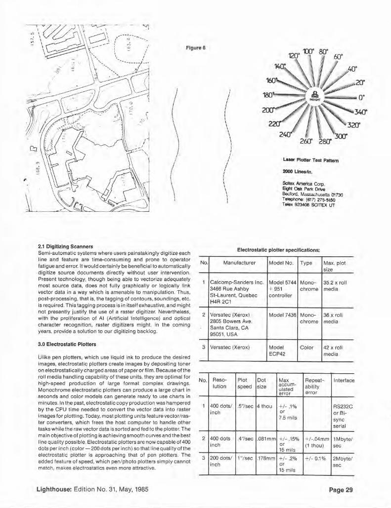
Figure 6

2.1 Digitizing Scanners Semi-automatic systems where users painstakingly dig it ize each line and feature are time-consuming and prone to operator fatigue and error. It would certainly be beneficial to automatically digitize source documents directly without user intervention. Present technology, though being able to vectorize adequately most source data, does not fully graphically or logical ly link vector data in a way which is amenable to manipu lation. Thus, post-processing, that is, the tagging of contours, soundings, etc. is requ ired. This tagging process is in itself exhaustive, and might not presently justify the use of a raster digitizer. Nevertheless, with the proliferation of AI (Artificial Intelligence) and optical character recognit ion, raster digitizers might, in the coming years, provide a solution to our digitizing backlog.

3.0 Electrostatic Plotters

Ulike pen plotters, which use liquid ink to produce the desired images, electrostatic plotters create images by depositing toner on electrostatically charged areas of paper or film. Because of the rol l media handling capability of these units, they are optimal for high-speed production of large format complex drawings. Monochrome electrostatic plotters can produce a large chart in seconds and color models can generate ready to use charts in minutes. In the past, electrostatic copy production was hampered by the CPU time needed to convert the vector data into raster images for plotting. Today, most plotting units feature vector/ ras­ter converters, which frees the host computer to handle other tasks while the raw vector data is sorted and fed to the plotter. The main objective of plotting is achieving smooth curves and the best line quality possible. Electrostatic plotters are now capable of 400 dots per inch (color- 200 dots per inch) so that line quality of the electrostatic plotter is approach ing that of pen plotters. The added feature of speed, which pen/ photo plotters simply cannot match, makes electrostatics even more attractive.

Lighthouse: Edition No. 31 , May, 1985

No.

1

2

3

No.

1

2

3

; I I

I I I I I I I I I I I I I I I I I I

I I

I I I I I I I I I I I I

L.aaw Plotter Test Pattern

2000 Lines/ln.

Scitex America Corp. Eight Oak Park Drive Bedford, Massachusetts 01730 Telephone: (617) 275-5150 Telex 923408 SCITEX UT

Electrostatic plotter specifications:

Manufacturer Model No. Type Max. plot size

Calcomp-Sanders Inc. Model5744 Mono- 35.2 x roll 3466 Rue Ashby + 951 chrome media St-Laurent, Quebec controller H4R 2C1

Versatec (Xerox) Model 7436 Mono- 36 x roll 2805 Bowers Ave. chrome media Santa Clara, CA 95051, USA

Versatec (Xerox) Model Color 42 x roll ECP42 media

Reso- Plot Dot Max Repeat- Interface lution speed size accum- ability ulated

error error

400 dots/ .5"/sec 4thou +1- .1% RS232C inch or or Bi-

7.5 mils sync serial

400 dots .4'Ysec .081mm +!- .15% +l- .04mm 1 Mbyte/ inch or (1 thou) sec

15 mils

200 dots/ 1 "/sec .178mm +!- .2% +!- 0.1% 2M byte/ inch or sec

15 mils

Page 29

No. Servicing/maintenance

1 - 3 months warranty - local Ottawa service - maintenace costs: plotter $325/ month controller $396/month

Costs

plotter: control ler:

total cost

$ 59,765.00 $ 39,510.00

$ 99,275.00

numerous, so discussion has been limited to the better known and used plotters, which can accomodateour large format charts. Determining factors were cost, user-friendliness, ease/ speed of interface, reliability, local servicing, number of pens (number of colors) and overall functionality.

Multi-Pen specifications.

2 - 3 months warranty plotter: $ 73,500.00 No. Manufacturer Model Pen Type #of Interface -full service: control ler: $ 23,000.00 $4,360.00/annum 40Mb disk: $ 14,750.00

1/0: $ 3,400.00

total cost $114,650.00

3 - 3 months warranty plotter: $152,000.00 -full service: controller: $ 23,000.00 $9,690.00/annum 40Mb disk: $ 21,000.00

1/ 0: $ 3,400.00

total cost $199,400.00

4.0 pen Plotters In our future application environment which provides for interac­t ive color editing, it would be desirable (based on cartographer dialog) to also provide a form of color verification plotting. A multi-pen (multi-color) plotter can accommodate our require­ments by way of distinctive color contouring and area cross­hatch ing. With these two features, an adequate full color emu­lated verification plot can be generated which could fulfill our cartographers' needs. The main advantage of the multi- pen plot­ter (over electrostatic) is cost, be it at a tremendous sacrifice in plotting throughout Color area fills will have to be emulated by way of cross-hatching so as not to increase plotting time unrea­sonably. The range of plotters which satisfies these features is

No. Resolution .Standard features Speed

1 0.5 thou -plot limits, skew up to 42 ips and size compensation - scale, rotate and mirror

2 0.98 thou -line, arc, intern~! 5.98 ips character generation - rotation/ scaling of 14ips symbols - mirroring, skew 14ips and compensation

3 0.98 thou - graphics instruc- up to 24 ips lion set available - 18kbyte buffer -international or user defined charac-

. ter set

4 0.5 thou - windowing up to 35 ips - 2K buffer - self diagnostics -single vector operation

Page 30

pens

1 Calcomp-Sanders 965 - liquid ink 4 RS232C 19.2 401 Champagne - ny lon tip kbaud Drive - ballpoint Downsview, Ontario

2 Calcomp-Sanders 1042 - ballpoint 8 RS232C - liquid ball IEEE488

1043 -nylon tip - liquid tip

1044 (option: $670)

3 Hewlett-Packard HP7585B - fiber tip 8 RS232C 2670 Queensview - rol ler ball 9600 baud or Drive HP7586B -drafting pen HPIB X on/-Ottawa, Ontario Xoff or hard-K2B 8K1 ware hand-

shaking

4 Nicolet-Zeta 3620 - liquid rolle 4 RS232C 19.2 1-1200 Aerowood -nylon tip kbaud or IEEE Drive -bal lpoint 488 (option) Mississauga, Ontario -liquid ink L4W 2S7

Plotting Area Accuracy

34 X 59.7" +1- .1"

34 X 46.96"

36.5 X 48" +1- .1%

34" X 240" +1- 0.5mil

Lighthouse: Edit ion No. 31, May, 1985

7RISPONDER. ~~~sYSTEMs~~~~

The Name for Accuracy and Reliability

Line of sight and beyond, Del Norte Technology, Inc., makes a TRISPONDER® System to do your job with repeatable accuracy and reliability- and a track record to prove it.

Del Norte's state-of-the-art micro­processor controlled equipment provides

Features common to all TRISPONDER Systems include:

• Extremely "operator friendly"

• 80 codes • Multi-user operation • One tenth meter

instrumental resolution • Operator selectable baud rates • Standard serial output with

BCD available as an option • Update rates are variable from

one half second to five seconds • All ranges are automatically

deskewed by microprocessor • Free standing or rack mounted • External host computer control

(Download) • Automatic multi-baseline

function

Del Norte has been the sole designer and manufacturer of all precision TRISPONDER Systems for over 16 years. A high-technology company dedi­cated to designing systems to meet your needs.

a broad range of measuring and positioning capabilities and functions. Units are

lightweight, highly portable, waterproof and consume very low power. They automatically power down when they are not being interrogated.

Model 520- 80 km line-of-sight • 2 range display- 4 range

output • Waterproof- unit floats

Model 542- 80 km line-of-sight • 4 range display and output • Guidance package standard

Model562 • 8 range output -waterproof

Model547/567 UHF­Over the horizon 2-3 times line-of-sight • 4 range display and output

For pinpoint accuracy- try Del Norte TRISPONDER

Systems - proven reliability at an afford­able price. Write for descriptive literature with detailed specifi­

Model547 cations. UHF All Systems are

FCC type approved.

TRISPONDER"' is a registered trademark of Del Norte Technology, Inc.

E@ DEL NORTE Technology, Inc. 1100 Pamela Drive, P.O. Box 696, Euless, Texas 76039,817/267-3541 Telex 75844-3

©1 984 Del Norte Technology, Inc.

No. Repeatabi I ity Media Cost

1 +I- 5 thou -translucent $32,165 - mylar -vellum - rag - preprinted fi lms

2 - translucent $12,090 - 100% rag -vellum $12,090 - 1411 paper -film $17,815

3 +1- 4 thou -paper $23,226 -vellum tracing bond $30,110 - films

4* +1- 1 mil -translucent $59,435 -vellum -mylar - clear acetate

-All plotters come with callable functional subroutines (optional*)

5.0 Summary

5.1 Raster

The raster (scanner) types of plotters is leading the way in high­tech plotting . Its growing popularity is due to such features as unlimited symbology, inherent reliability, good line density/­quality and a high plotting throughput. The SCITEX ELP has shown the most promise. It sports excellent accuracy and repeat­ability specifications, as well as sound electrical/mechanical design. SCITEX is presently supporting its plotters from Montreal and Toronto, and with the increased number of Ottawa users, plans are in the works for local support. The ELP can be upgraded (option) to support input scanning, an area which might prove beneficial. The output line/symbol work has very good contrast, density and a more than adequate quality.

5.2 Mu lti-pen

To satisfy our requirements for verification plotters, the author has recommended the HP7586B, primarily since our next genera­tion of software supports an HP manufactured plotter. The HP7586B accommodates our required verification accuracy and repeatability, while maximizing color availability(8 pens). Hewlett­Packard is world-renowned for its pen plotters. It has become the de-facto standard pen plotter in many CAD shops. The HP7586B is serviced locally, provides access to 15 user-callable Fortran subroutines (such as polygon fill) while supplying an 18Kbyte buffer for host overhead reduction. International or user-defined character sets are featured/downloadable on this plotter. The plotter provides a user-friendly display/control panel and a proven paper moving technology (minimizes problem sources: the physics of control and resonance phenomena, the inertia versus power concerns, and stability). The HP7586B has a power­ful graphics instruction set, but does suffer slightly in its maxi­mum 9600 baud communication rate (RS232C). The $30K price tag of the HP7586B falls in the middle of the pen plotter cost spectrum. A reduction to $23,226 is possible with the single sheet

Page 32

Service Other features

local: $214/month - USCR (user selected curve resolution) - arc generated characters

local: $105/month - ROMpack local: $105/month firmware local: $130/month - pen turret

- HCBS software - control panel

- error recovery with block mode data transfer - built in calibration routine

1 year parts and - Automatic test labour patterns

- controllable pen speed and pressure

media model (roll media not required). With capital cost as prime factor, the Calcomp-Sanders 1044 ($17,815) fills the bill. It has comparable accuracy and repeatability specifications (with the HP7586B) but does suffers from a slower plotting speed (HP7586B:24 ips vs. Calcomp 1044: 14 ips). Nevertheless, it comes with an extensive user callable subroutine package.

5.3 Electrostatic

The electrostatic plotter is substantially faster than multiple-pen plotters and much more colorful. To use it as a verification plotter could not be justified due to the relatively high cost. However, as a "final product" plotter, the electrostatic offers exciting potential as a next generation output-hardcopy device. Over the past decades, much effort has been made to automate the chart gen­erating process. Hardcopy (paper chart) production has been provided by lithographic processes. Unfortunately, these pro­cesses have introduced their own set of errors and idiosyncrasies. The present method of printing (press) can yield a +1-0.005 registration error and up to 0.25 inch absolute error over the span of the chart. Alternatively, the Versatec color electrostatic plotter has half the registration error and a maximum accumulated error of 0.015 inch (or+!- 0.1%), a factor 3 to 10 times better. The electrostatic method would also eliminate errors from the other lithographic processes (i.e. plate production). To make printing by press cost-effective usually requires large runs, that is, a large number of charts printed, whereas rasterizing time needed, that is, the vector to raster conversions, is but a small percentage of the present lithographic processing time. Lithography is also very costly for it needs much specialized equipment, qualified person­nel to run it, special environments (humidity/temperature control, dark-room) to work in and continual upkeep. A present (Versatec) installation, BNR (Bell Northern Research), is producing color and monochrome electrostatic plots (Integrated Circuits) 24 hours a day, 6 to 7 days a week. They have been doing so for the past 8 months without failure, in an existing computing en­vironment.

Lighthouse: Edition No. 31, May, 1985

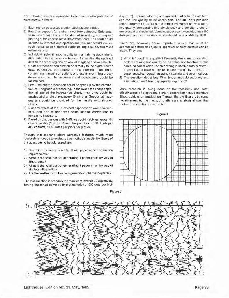
The fol lowing scenario is provided to demonstrate the potential of electrostatic plotters:

1) Each region possesses a color electrostatic plotter. 2) Regional support for a chart inventory database. Said data­

base would keep track of local chart inventory, and request plotting of the charts that fall below set limits. The limits could be fixed by interactive projection analysis, and would include such variables as historical statistics, regional development estimates, etc.

3) Individual regional responsibility for maintaining stock labels, distribut ion to their sales centers and for sending the updated data to the other regions by way of magtape and/or satellite.

4) Chart corrections could be made directly to the digital vector data (CARED ), re-rasterized and plotted. The time­consuming manual corrections or present re-printing proc~­dures would not be necessary and consistency could be maintained.

5) First-time chart production could be sped up by the elimina­tion of lithographic processing. In the event of a sharp deple­tion of one of the inventoried charts, new ones could be produced at a rate of one every 10 minutes. Support at head­quarters could be provided for the heavily requisitioned charts.

6) Disposal waste of the un-revised paper charts would be min­imal, and non-existent with some manual corrections to remaining inventory.

7) Based on discussions with BNR, we could viably generate 144 charts per day (3 shifts, 10 minutes per plot) or 108 charts per day (2 shifts, 10 minutes per plot) per plotter.

Though this scenario offers attractive features, much more research is needed to evaluate this method 's feasibility. Some of the questions to be addressed are:

1) Can this production leve l fulfill our paper chart production requirements?

2) What is the total cost of generating 1 paper chart by way of I it hog raphy?

3) What is the total cost of generating 1 paper chart by way of electrostatic plotter?

4) Are the aesthetics of this new generation chart acceptable?

The last question is probably the most controversial. Subjectively, having examined some color plot samples at 200 dots per inch

(Figure 7), I found color registration and quality to be excellent, and the line quality to be acceptable. The 400 dots per inch (monochrome: Figure 8) plot samples (Versatec) showed good line quality, comparable line consistency and density to one of our present printed chart. Versatec are presently developing a 400 dots per inch color version, which should be available by 1986.

There are, however, some important issues that must be addressed before an objective appraisal of electrostatics can be made. They are:

1) What is "good" line quality? Presently there are no standing orders defining line quality or the actual line location versus sampled points when line smoothing is used (photo-plotters). These issues have solely been determined by a group of experienced cartographers using visual trial and error methods.

2) The quest ion also arises: What importance do accuracy and aesthetics have? Are they equally important?

More research is being done on the feasibility and cost­effectiveness of electrostatic chart generation versus standard lithographic chart production. Though there will surely be some negativeness to the method, preliminary analysis shows that further investigation is warranted.

Figure 8

- 1P'

v -1

-

-

-

-~

- ~

" r I I I I I

Figure 7

5 .

6 .

Lighthouse: Edition No. 31, May, 1985 Page 33

References 1) "The Computer in Contemporary Cartography", Vo11, Edited

by D.R. Fraser Taylor. 2) "Digital Film Plotters provide fast hardcopy at cost-effective

rates", by David Nims, Computer Technology Review, Sum­mer 1984.

3) "Electrostatic Plotters capture the big picture", Thomas A. Nobbe, Machine Design, March 21, 1985.

4) "High speed, large format flatbed photocomposition system", P.F. Grosso, Proceedings Auto-Carto IV, November 408, 1979.

5) "Higher Plotting Resolution: is it worth the money?", David Kenney, Computer Graphics World, January 1985.

6) "Computer Assisted Cartography and Geographic Informa­tion Processing: Hope and Realism", David H. Douglas and A.R. Boyle - editors, Canadian Cartographic Association, 1982.

7) "Computer Mapping: progress in the 80's', James R. Carter, Association of American Geographers, 1984.

8) "Computer Applications: Cartographic Drawing with Compu­ters", P. Yoeli, Special Issue of Computer Application , Vol 8, 1982.

Figures 1 to 4 were reproduced from reference 2.

Figure 5 was provided by Lands Directorate, Environment Canada

Figure 6 was provided by Scitex Canada Inc.

Figures 7 and 8 were provided by Versatec (a Xerox company)

Page 34 Lighthouse: Edition No. 31, May, 1985

Atlas Polarfix A dynamic range/azimuth measurement system for ships,

dredgers and rigs - more accurate, simpler, more cost-effective. The solution for short range position-fixing.

Prism reflecto r assembly

This completely new laser position­fixing system has many advantages over the conventional microwave methods:

• Greater accuracy, ± 20 cm/km

• No limitations imposed by inter­section angle geometry

• None of the measurement errors and interference problems asso­ciated with radio position-fixing methods

• Only one shore station

• Automatic target-tracking and target-seeking

• Data transmission and remote control of functions by means of telemetry

• Infrared laser with a range of 5 km approximately

• Simple system-integration, thanks to standardised interfaces

Atlas Polarfix -reliable and trend-seHing. Krupp Atlas survey systems, based on experience to give dependability, ruggedness and economy throughout a long life.

We'd be glad to tell you more. Have a word with us!

KRUPP ATLAS ELEKTRONIK­A SOUND DECISION.

~ KRUPP ATLAS ELEKTRONIK Krupp International Inc. · Krupp Atlas Elektronik Division

1453 Pinewood Street· Rahway, New Jersey 07065 · USA · Phone 2013881500 ·Telex 7109965843 krupp rway

ON TARGET POSITIONING 8c TRACKING

SYSTEMS

A vast array of systems:

Electronic Distance Measuring - infra-red - microwave -laser -acoustic

Electronic Range/Bearing - infra-red - microwave -laser

Electronic Positioning & Navigating -3 to 16 GHz microwave -400 MHz UHF -2 MHz ground wave - undersea acoustic

Vessel Traffic Control -survey navigation/guidance - remote vehicle tracking

Featuring Quality Products From: [I}{j,NJ[]

50 Doncaster Ave .. Unit B. Thornhill, Ontario Canada. L3T 1 L4 Tel. (416) 881-8551 Telex 06-964 514

li'f Sales li'f Service li'f Leasing

You need the best imaging sonar available. This is it - the 971. A colour imaging, multi­purpose miniature sonar. Best because it displays the widest range of signal levels. Because each of its 128 distinct colours represents a precise sound level. Because it has the highest defini­tion - 1:1 million pixels - to show the finest details. And because the colours and high definition produce breathtaking images. Perspective Mode: For Pilotage

Sector Mode: For Obstacle Avoidance

As shown here, the colours re­present about one tenth of the actual brilliance of the monitor screen. The sonar also displays a dynamic sequence of images, en­hancing your interpretation.

With the 971, you can 'see' as far as 100 metres. Compare that to a few metres with your eye or TV. Add the feature of f ive opera­ting modes/display formats and you have an unrivalled versatility. For instance. the narrow sonar beam of the Sector Scan will de­tect even the smallest hazards and the display will reveal them. Per­fectly. Switch to the unique Per-

spective Mode for Pilotage and a sound image of the outside world is presented with stunning realism. You 'fly ' into the scene guided by the perspective grid.

Switch to the Polar Scan Mode for General Survei llance. If a job calls for monitoring and control­ling traffic at an oil rig, this mode will guide divers and vehicles dir­ectly to a rendezvous or work sta­tion . Constant monitoring can be ach ieved with an NTSC or PAL converter and a standard video recorder. And playback utility is enhanced by the on-screen data, which lets you record date, time, depth ...

Side-Scan is well known, but the 971 's high definit ion colour display adds a completely new dimension. Surfaces are recog­nized by their signal strength , as shown by their colour. And targets which you miss with a regular so­nar's limited on-screen range show clearly on the 971 .

This much performance would normally requ ire a rack full of equipment. Not so with the 971 . The on-board processor is com-

Side Scan Mode: For Large Area Surveys

pact, the Sonar Head is small and yet light enough to f it any ROV. Or to pass through drill strings, casings and sea chests.

Performance, versatility, size, value. Now you know. No other sonar comes close.

2830 Huntington Place Port Coquitlam, B.C., Canada V3C 4T3 Tel. : (604) 464-81 44 Telex 04-353637

i ~ l

I

I I

I