Embed Size (px)
Citation preview

1Lptvaomlcwsart
btemivcnpn
mmblcaw
tdo
Stout et al. Vol. 22, No. 11 /November 2005 /J. Opt. Soc. Am. A 2385
Light diffraction by a three-dimensional object:differential theory
Brian Stout, Michel Nevière, and Evgeny Popov
Institut Fresnel, Unité Mixte de Recherche 6133, Case 161 Faculté des Sciences et Techniques, Centre de SaintJérôme, 13397 Marseille Cedex 20, France
Received January 31, 2005; accepted March 22, 2005
The differential theory of diffraction of light by an arbitrary object described in spherical coordinates is devel-oped. Expanding the fields on the basis of vector spherical harmonics, we reduce the Maxwell equations to aninfinite first-order differential set. In view of the truncation required for numerical integration, correct factor-ization rules are derived to express the components of D in terms of the components of E, a process that ex-tends the fast Fourier factorization to the basis of vector spherical harmonics. Numerical overflows and insta-bilities are avoided through the use of the S-matrix propagation algorithm for carrying out the numericalintegration. The method can analyze any shape and/or material, dielectric or conducting. It is particularlysimple when applied to rotationally symmetric objects. © 2005 Optical Society of America
OCIS codes: 290.5850, 050.1940, 000.3860, 000.4430.
mvstmstiiamcs
pmsldfsgsdttvnsmom
irttO
. INTRODUCTIONight scattering from arbitrarily shaped 3D objects com-arable in size to the wavelength of the scattering radia-ion is an important problem with applications covering aast range of fields of science and technology, includingstrophysics, atmospheric physics, radiative transfer inptically thick media such as paints and papers, and re-ote detection. By “comparable in size with the wave-
ength,” we are most often speaking of particles having aharacteristic size D within an order of magnitude of theavelength, � /10�D�10�. In this size regime, and for
catterers of sufficiently high dielectric contrast, popularpproximations such as the Rayleigh–Gans1,2 or geomet-ic optics approximations1,2 are invalid; one must resorto an essentially full solution of the Maxwell equations.
The first full solution to the electromagnetic scatteringy a fully 3D object is that of Lorenz and Mie for the scat-ering by a single homogeneous isotropic spherical objectmbedded in a homogeneous isotropic externaledium.3–5 This renowned solution takes the form of an
nfinite (but rapidly converging) series of coefficients in-olving spherical Bessel functions. Being the only analyti-ally manageable exact solution to the full electromag-etic scattering problem, the Mie solution has played areponderate role in light-scattering calculations forearly a century.In view of the size range in which the Mie theory isost useful, it comes as no surprise that Mie theory isost frequently applied to media containing a large num-
er of scattering inclusions. Since the Mie theory is a so-ution only to an isolated particle, it has frequently beenoupled with the independent scattering approximationnd applied to tenuous media systems containing only aeek volume density of scatterers.6
The increasing interest in recent decades of light scat-ering by aggregates and light propagation in dense me-ia such as composites, containing a high volume densityf inclusions, has fueled considerable progress in the
1084-7529/05/112385-20/$15.00 © 2
ultiple-scattering problem of such dense media.7–9 Iniew of the already considerable difficulty of the multiple-cattering equations, a majority of these studies have con-inued to use spheres as the fundamental scattering ele-ent. In reality, of course, it is extremely rare for
cattering inclusions to be so obliging as to separatehemselves into distinct compact spheres, even though anmpressive number of mechanical and chemical processesn a number of industries have been developed with ex-ctly this goal in mind (grinding, surfactants,…). Further-ore, it has long been clear that nonspherical inclusions
an yield quantitatively different results on the macro-copic scale than spherical inclusions.
Many multiple-scattering codes and theories have em-loyed with considerable success the notion of a transferatrix (frequently called the T matrix in the multiple-
cattering community; see the note10) that consists of ainear transformation between the excitation field inci-ent on a scatterer and the scattered field emanatingrom it.2,7–9,11 The transfer matrix is more than a singleolution to the scattering problem corresponding to aiven incident field; rather it can be viewed as a completeolution to the scattering problem for any possible inci-ent field. In the multiple-scattering theories employingransfer matrices, the Mie solution to the sphere takeshe form of a diagonal transfer matrix in a basis of theector spherical wave functions. It has long been recog-ized by those working in this field that nonsphericalcatterers can rather readily be integrated into existingultiple-scattering theories by simply replacing the diag-
nal Mie transfer matrices of spheres by the full transferatrices of nonspherical objects.There exist a number of techniques for treating scatter-
ng by nonspherical objects, but not all of these caneadily provide the complete solution required to derive aransfer matrix, and the reliability and applicability ofhese various techniques is a recurring stumbling bock.ne of the most popular techniques in the literature is
005 Optical Society of America

twcverthitla
ttfscdtgtaahtFlmVma
li4actlrcfa
2Frs�
o
Auns�
dmrtts�tt�w�
memgsr�
wm
Ttm
at
m
2386 J. Opt. Soc. Am. A/Vol. 22, No. 11 /November 2005 Stout et al.
he Waterman (or extended boundary condition) method,hose popularity is in large part due to the fact that one
an readily obtain from it a full transfer matrix for a largeariety of nonspherical shapes.12 It has been shown, how-ver, that the Waterman technique yields the same algo-ithm as one obtains from a Rayleigh hypothesis.11 Bothhe Rayleigh hypothesis and the Waterman techniqueave been demonstrated to have considerable limitations
n the theories of diffraction gratings,13 and it is well es-ablished that both the Waterman technique and the Ray-eigh hypothesis can break down for scatterers with highspect ratios.11
The above remarks have in part provided our motiva-ion to propose a new differential theory for deriving theransfer matrix of nonspherical scatterers. Although dif-erential theories have been studied previously for 3Dcatterers, we have developed our theory from first prin-iples and made full use of recent breakthroughs in theifferential theory of 1D, 2D, and 3D diffraction gratingshat have greatly improved the reliability and conver-ence of differential theories. The new methods in ques-ion have been presented and elaborated in a number ofrticles14–19 and a recent book,20 but these works are notprerequisite for understanding the present work, whichas been conceived to be self-contained. The differentialechnique in diffraction gratings makes extensive use ofourier series, and their extension to the 3D problem
eads us to make considerable use of vector spherical har-onics (VSHs) in the derivation of our formulas. TheSHs, however, do not appear in the final computationalethod, and the finer details of the VSH manipulations
re provided in Appendix C.The work is organized as follows. We present the prob-
em in Section 2. We introduce the VSHs in Section 3 andntroduce their applications to field expansions in Section. The propagation equations are derived in Section 5,nd the fast numerical factorization (FNF) required foronvergence of the series is thoroughly discussed in Sec-ion 6. We study field developments outside the modu-ated region in Section 7 and present the prescription foresolving the boundary-value problem in Section 8. Weonclude this work by briefly illustrating the necessaryormula for extracting physically relevant quantities suchs cross sections and scattering matrices.
. PRESENTATION OF THE PROBLEMigure 1 shows a finite object, made of an isotropic mate-ial, with arbitrary shape limited by a surface �S�. Thisurface is described in spherical coordinates �r ,� ,��, with� �0,�� defined in the figure by the equation
f�r,�,�� = 0 �1�
r
r = g��,��. �2�
t a given point M on the surface, the external normalnit vector is N, and the unit vectors of spherical coordi-ates are denoted r, �, �. The surface �S� divides thepace into two regions. The first region, contained withinS�, is filled with a linear, homogeneous, and isotropic me-
ium, dielectric or conducting, described by complex per-ittivity �1. The second region lies outside �S� and has
eal permittivity �m. In view of developing the differentialheory, we divide space into three regions by introducinghe inscribed sphere �S1� with radius R1 and the circum-cribed sphere �S2� with radius R2; the region betweenS1� and �S2� is called the “modulated region,” a denota-ion that recalls that for any constant value r0 of r be-ween R1 and R2, the permittivity, �, is a function of � andand, furthermore, is obviously periodic with respect to �ith a period of 2� and piecewise constant with respect toand �.The object is subject to an incident harmonic electro-agnetic field described by its electric field, Ei, with an
xp�−i�t� time dependence. As is well known in quantumechanics and electromagnetism,21–23 any function of an-
ular variables � and � can be developed on the basis ofcalar spherical harmonics Ynm�� ,��. The dimensionlesselative dielectric constant, ��r ,� ,��, defined such that0��r ,� ,�����r ,� ,�� can therefore be expressed as
��r,�,�� = �n=0
�m=−n
n
�nm�r�Ynm��,��, �3�
hich implies that �nm�r� can be obtained from the Her-itian product:
�nm�r� = �Ynm�� � 0
4�
Ynm* ��,����r,�,��d. �4�
he reader should note that in Eq. (4) and throughouthis work we have adopted the convention for scalar Her-itian products such that
�g�f � g*�x�f�x�dx. �5�
In Eq. (4), the asterisk denotes the complex conjugate,nd is the solid angle. Equation (4) can thus be rewrit-en as
�nm�r� =0
2� 0
�
��r,�,��Ynm* ��,��sin �d�d�. �6�
A development of the vector electromagnetic field is aore complicated affair. One might first be tempted to ex-
Fig. 1. Description of the diffracting object and notations.

pfistasi
3Vtt(ftt
w
Aio
wpar
Yf
om
I
w
Esa�
rtg
4Ad
Stpnma�ft
w
Stout et al. Vol. 22, No. 11 /November 2005 /J. Opt. Soc. Am. A 2387
and each spherical coordinate component of the totaleld �E ,H� on the basis of the scalar spherical harmonics,imilar to Eq. (3). But when such expansions are put intohe Maxwell equations, derivatives of the Ynm functionsrise that are difficult to calculate and manipulate. Con-equently, we choose another way to expand vector fields;.e., we represent them on the basis of VSHs.
. VECTOR SPHERICAL HARMONICSSHs are described in several reference books,6,21–23 al-
hough their definitions and notations vary with the au-hors. They arise in vector solutions of the wave equationHelmholtz equation) and when appropriately defined canorm an orthogonal complete basis to represent the elec-romagnetic field. We choose to define and denote them byhe following equations:
Ynm��,�� � rYnm��,��, �7�
Xnm��,�� � Znm��,�� � r , �8�
here
Znm��,�� �r � Ynm��,��
�n�n + 1�
if n � 0, Z00��,�� � 0. �9�
Equation (8) implies that
Znm��,�� = r � Xnm��,��. �10�
ll the VSHs are mutually orthonormal in the sense thatf Wnm
�i� (i=1, 2, 3) denotes the vector harmonics Ynm, Xnm,r Znm, we have
�Wnm�i� �W�
�j� � 0
4�
Wnm�i�* · W�
�j� d = �ij�n��m , �11�
here �ij is the Kronecker symbol and the Hermitianroduct of Eq. (4) has been extended to vector fields. Welso remark from Eqs. (7)–(9) that if the Wnm
�i� �� ,�� wereeal the trihedral �Ynm ,Xnm ,Znm� would be direct.
Let us recall that the scalar spherical harmonicsnm�� ,�� are expressed in terms of associated Legendre
unctions Pnm�cos �� as23
Ynm��,�� = �2n + 1
4�
�n − m�!
�n + m�! 1/2
Pnm�cos ��exp�im��
�12�
r by including the square root in the definitions of nor-alized associated Legendre functions Pn
m:
Ynm��,�� = Pnm�cos ��exp�im��. �13�
ntroducing functions unm and sn
m defined by
unm�cos �� =
1
�m
sin �Pn
m�cos ��, �14�
n�n + 1�snm�cos �� =
1
�n�n + 1�
d
d�Pn
m�cos ��, �15�
e can express the vector harmonics Xnm and Znm as
Xnm��,�� = iunm�cos ��exp�im��� − sn
m�cos ��exp�im���,
�16�
Znm��,�� = snm�cos ��exp�im��� + iun
m�cos ��exp�im���.
�17�
quations (16) and (17), combined with Eq. (7), clearlyhow that for a given n, m the �Ynm ,Xnm ,Znm� are mutu-lly perpendicular in the sense that Wnm
�i� ·Wnm�j� =0 for i
j.Other interesting relations are the curl of products of a
adially dependent function h�r� by a Wnm�i� . These rela-
ions will prove to be useful in the derivation of the propa-ation equations and are given by
curl�h�r�Ynm� = �n�n + 1��1/2h�r�
rXnm, �18�
curl�h�r�Xnm� =h�r�
r�n�n + 1��1/2Ynm + �h�r�
r+ h��r� Znm,
�19�
curl�h�r�Znm� = − �h�r�
r+ h��r� Xnm. �20�
. FIELD EXPANSIONSn arbitrary vector field U�r ,� ,�� can be expressed in aevelopment of the VSHs as stated by
U�r,�,�� = �n=0
�m=−n
n
�AYnm�r�Ynm��,�� + AXnm�r�Xnm��,��
+ AZnm�r�Znm��,���. �21�
uch a development will be subsequently applied to theotal electric field E, the total magnetic field H, the dis-lacement D, the incident electric field Ei, and the unitormal vector N. However, in view of a numerical treat-ent, the summation in Eq. (21) will have to be limited tovalue of n equal to nmax. Also, the double subscript
n ,m� will be replaced by a single subscript p, varyingrom 1 to N. It is then easy to establish that Eq. (21) takeshe form
U�r,�,�� = �p=1
N
�AYp�r�Yp��,�� + AXp�r�Xp��,��
+ AZp�r�Zp��,���, �22�
here N��n +1�2 and
max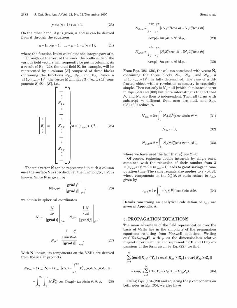
Of
w
varc�p
ok
w
Wf
Fc�fsiNs(
w
c�pwg
Dg
5Tbecmp
b
2388 J. Opt. Soc. Am. A/Vol. 22, No. 11 /November 2005 Stout et al.
p = n�n + 1� + m + 1. �23�
n the other hand, if p is given, n and m can be derivedrom it through the equations
n = Int�p − 1, m = p − 1 − n�n + 1�, �24�
here the function Int�x� calculates the integer part of x.Throughout the rest of the work, the coefficients of the
arious field vectors will frequently be put in columns. Asresult of Eq. (22), the total field E, for example, will be
epresented by a column �E� composed of three blocksontaining the functions EYp, EXp, and EZp. Since p
�1, �nmax+1�2�, the vector E will have 3� �nmax+1�2 com-onents El :E↔ �E�, i.e.,
� ]
El
]
� ���—
]
EY,p
]
—
]
EX,p
]
—
]
EZ,p
]
—
��3 � �nmax + 1�2. �25�
The unit vector N can be represented in such a columnnce the surface S is specified; i.e., the function f�r ,� ,�� isnown. Since N is given by
N��,�� = � grad f
�grad f��
f=0
, �26�
e obtain in spherical coordinates
Nr = ��f
�r
�grad f��
f=0
, N� = �1
r
�f
��
�grad f��
f=0
,
N� = �1
r sin �
�f
��
�grad f��
f=0
. �27�
ith N known, its components on the VSHs are derivedrom the scalar products
NYnm = �Ynm�N = �Ynmr�rNr =0
4�
Ynm* ��,��Nr��,��d
=0
2� 0
�
NrPnm�cos ��exp�− im��sin �d�d�, �28�
NXnm =0
2� 0
�
�iN�unm�cos �� − N�sn
m�cos ���
�exp�− im��sin �d�d�, �29�
NZnm =0
2� 0
�
�N�snm�cos �� + iN�un
m�cos ���
�exp�− im��sin �d�d�. �30�
rom Eqs. (28)–(30), the column associated with vector N,ontaining the three blocks NYp, NXp, and NZp, p
�1, �nmax+1�2�, is fully determined. The case of a dif-racted object with a revolution symmetry is especiallyimple. Then not only is N� null [which eliminates a termn Eqs. (29) and (30)] but more interesting is the fact that
r and N�, are then � independent. Then all terms withubscript m different from zero are null, and Eqs.28)–(30) reduce to
NYn0 = 2�0
�
Nr���Pn0�cos ��sin �d�, �31�
NXn0 = 0, �32�
NZn0 = 2�0
�
N����sn0�cos ��sin �d�, �33�
here we have used the fact that un0�cos ��=0.
Of course, replacing double integrals by single ones,ombined with the reduction of their number from 3
�nmax+1�2 to 2� �nmax+1� leads to great savings in com-utation time. The same remark also applies to ��r ,� ,��,hose components on the Yn
m�� ,�� basis reduce to �n,0,iven by
�n,0 = 2�0
�
��r,��Pn0�cos ��sin �d�. �34�
etails concerning an analytical calculation of �n,0 areiven in Appendix A.
. PROPAGATION EQUATIONShe main advantage of the field representation over theasis of VSHs lies in the simplicity of the propagationquations resulting from Maxwell equations. Writingurl E= i� 0H, with as the dimensionless relativeagnetic permeability, and representing E and H by ex-
ansions of the form given by Eq. (22), we find
�p=1
N
�curl�EYp�r�Yp� + curl�EXp�r�Xp� + curl�EZp�r�Zp��
= i� 0�p=1
N
�HYpYp + HXpXp + HZpZp�. �35�
Using Eqs. (18)–(20) and equating the p components onoth sides in Eq. (35), we also have

jZ
S
as�
Thnst
F
w
M
(�tenmsk
tb
wpd
Stout et al. Vol. 22, No. 11 /November 2005 /J. Opt. Soc. Am. A 2389
�n�n + 1�EYp�r�
rXp + �n�n + 1�
EXp�r�
rYp + �EXp�r�
r
+dEXp�r�
dr Zp − �EZp�r�
r+
dEZp�r�
dr Xp
= i� 0�HYpYp + HXpXp + HZpZp�. �36�
Introducing ap=�n�n+1�, where n=Int�p−1, and pro-ecting both members of Eq. (36) on vectors Yp, Xp, andp, we obtain
ap
EXp
r= i� 0HYp, �37�
ap
EYp
r−
EZp
r−
dEZp
dr= i� 0HXp, �38�
EXp
r+
dEXp
dr= i� 0HZp. �39�
imilarly, the Maxwell equation, curl H=−i�D leads to
ap
HXp
r= − i�DYp, �40�
ap
HYp
r−
HZp
r−
dHZp
dr= − i�DXp, �41�
HXp
r+
dHXp
dr= − i�DZp. �42�
Since we work in linear optics �D=�0�E�, and since End D are represented on the same basis, there exists aquare matrix Q� that links the column �E� to the columnD� such that
�D� = �0Q��E�. �43�
his Q� matrix is made of nine square blocks, each blockaving dimension �nmax+1�2, which depend on the compo-ents of � defined in Eq. (6), and will be calculated in Sub-ection 6.C. We represent Q� by the following block struc-ure:
Q� = �Q�YY Q�YX Q�YZ
Q�XY Q�XX Q�XZ
Q�ZY Q�ZX Q�ZZ� . �44�
rom Eqs. (43) and (44), we thus obtain
1
�0�DY� = Q�YY�EY� + Q�YX�EX� + Q�YZ�EZ�, �45�
hich gives
�EY� = �Q�YY�−1� 1
�0�DY� − Q�YX�EX� − Q�YZ�EZ�� . �46�
oreover,
1
�0�DX� = Q�XY�EY� + Q�XX�EX� + Q�XZ�EZ�, �47�
1
�0�DZ� = Q�ZY�EY� + Q�ZX�EX� + Q�ZZ�EZ�. �48�
We first insert Eq. (40) into Eq. (46). We then insert Eq.46) into Eqs. (47) and (48) in order to express �DX� andDZ� in terms of �EX�, �EZ�, and �HX�, expressions that arehen inserted into Eqs. (41) and (42). In Eq. (41) �HYp� isliminated thanks to Eq. (37). In Eq. (38) �EY� is elimi-ated thanks to Eqs. (40) and (46). Introducing a diagonalatrix a with elements ap�p,q, we finally reduce the set of
ix equations, Eqs. (37)–(42), to four equations with un-nowns EXp, EZp, HXp, and HZp only:
EXp
r+
dEXp
dr= i� 0HZp �49�
ap
r��Q�YY�−1� ia
��0r�HX� − Q�YX�EX� − Q�YZ�EZ� �
p
−EZp
r−
dEZp
dr= i� 0HXp, �50�
HXp
r+
dHXp
dr= − i��0�Q�ZX�EX��p − i��0�Q�ZZ�EZ��p
− i��0�Q�ZYQ�YY−1 � ia
��0r�HX� − Q�YX�EX�
− Q�YZ�EZ���p
, �51�
iap
2
� 0
EXp
r2 +HZp
r+
dHZp
dr= i��0�Q�XX�EX��p
+ i��0�Q�XZ�EZ��p
+ i��0�Q�XYQ�YY−1 � ia
��0r�HX�
− Q�YX�EX� − Q�YZ�EZ���p
.
�52�
It is now useful to construct a column �F� containinghe unknowns of the problem, made with four blocks, eachlock having �nmax+1�2 components:
�F� = ��EX�
�EZ�
�HX�
�HZ�� , �53�
here the tilde means that the magnetic field is multi-lied by the vacuum impedance Z0 so that it has the sameimension as an electric field:
Tw
wbc
w
TmbetHTmhacgtdn
btdnsjc
6ABTltettEaiE
dGivdtsdpgtffatb
ALvpfifb=pv
1Iw
Isp
2390 J. Opt. Soc. Am. A/Vol. 22, No. 11 /November 2005 Stout et al.
H � Z0H =� 0
�0H =
1
c�0H. �54�
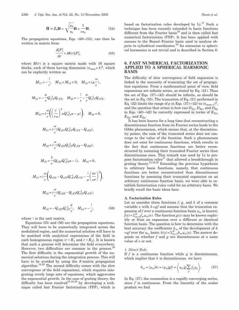
he propagation equations, Eqs. (49)–(52), can then beritten in matrix form:
d�F�
dr= M�r��F�, �55�
here M�r� is a square matrix made with 16 squarelocks, each of them having dimension �nmax+1�2, whichan be explicitly written as
M11 = −1
r, M12 = M13 = 0, M14 = i
�
c1,
M21 = −a
rQ�YY
−1 Q�YX, M22 = −1
r−
a
rQ�YY
−1 Q�YZ,
M23 = i�
c�� c
r��2
aQ�YY−1 a − 1�, M24 = 0,
M31 = i�
c�Q�ZYQ�YY
−1 Q�YX − Q�ZX�,
M32 = i�
c�Q�ZYQ�YY
−1 Q�YZ − Q�ZZ�,
M33 =1
r�Q�ZYQ�YY
−1 a − 1�, M34 = 0,
M41 = i�
c�Q�XX − Q�XYQ�YY
−1 Q�YX −1
� ac
�r�2� ,
M42 = i�
c�Q�XZ − Q�XYQ�YY
−1 Q�YZ�,
M43 = − Q�XYQ�YY−1
a
r, M44 = −
1
r, �56�
here 1 is the unit matrix.Equations (55) and (56) are the propagation equations.
hey will have to be numerically integrated across theodulated region, and the numerical solution will have to
e matched with analytical expressions of the field inach homogeneous region (r�R1 and r�R2). It is knownhat such a process will determine the field everywhere.owever, two difficulties are common in the process.20
he first difficulty is the exponential growth of the nu-erical solutions during the integration process. This willave to be avoided by using the S-matrix propagationlgorithm.14,20 The second difficulty comes with the slowonvergence of the field expansions, which requires inte-rating overly large sets of equations, which aggravateshe exponential growth. In the case of grating theory, theifficulty has been resolved15,16,20 by developing a tech-ique called fast Fourier factorization (FFF), which is
ased on factorization rules developed by Li.17 Such aechnique has been recently extended to basis functionsifferent from the Fourier basis18 and is then called fastumerical factorization (FNF). It has been applied withuccess to the Bessel–Fourier basis used to analyze ob-ects in cylindrical coordinates.19 Its extension to spheri-al harmonics is not trivial and is described in Section 6.
. FAST NUMERICAL FACTORIZATIONPPLIED TO A SPHERICAL HARMONICASIShe difficulty of slow convergence of field expansion is
inked to the necessity of truncating the set of propaga-ion equations. From a mathematical point of view, fieldxpansions are infinite series, as stated by Eq. (21). Thushe set of Eqs. (37)–(42) should be infinite, as should behe set in Eq. (55). The truncation of Eq. (21) performed inq. (22) limits the range of p in Eqs. (37)–(42) to �nmax+1�2,nd the question that arises is how can DYp, DXp, and DZpn Eqs. (40)–(42) be correctly expressed in terms of EYp,
Xp, and EZp.It has been known for a long time that reconstructing a
iscontinuous function from its Fourier series leads to theibbs phenomenon, which means that, at the discontinu-
ty points, the sum of the truncated series does not con-erge to the value of the function. Such a phenomenonoes not exist for continuous functions, which results inhe fact that continuous functions are better recon-tructed by summing their truncated Fourier series thaniscontinuous ones. This remark was used by Li to pro-ose factorization rules17 that allowed a breakthrough inrating theory.15,16,20 Extending the previous hypothesiso arbitrary basis functions, namely, that continuousunctions are better reconstructed than discontinuousunctions by summing their truncated expansion on anrbitrary continuous function basis, we were able to es-ablish factorization rules valid for an arbitrary basis. Weriefly recall the basic ideas here.
. Factorization Ruleset us consider three functions f, g, and h of a commonariable x with h=gf and assume that the truncation ex-ansion of f over a continuous function basis �m is known:�x�=�m=1
N fm�m�x�. The function g�x� may be known explic-tly or from an expansion over a different or identicalunction basis. The question is how to determine with theest accuracy the coefficients hm of the development of hgf over the �m basis: h�x�=�m=1
N hm�m�x�. The answer de-ends on whether f and g are discontinuous at a samealue of x or not.
. Direct Rulef f is a continuous function while g is discontinuous,hich implies that h is discontinuous, we have
hm = ��m�h = ��m�gf = ��m�g�p
fp�p� . �57�
n Eq. (57), the summation is a rapidly converging series,ince f is continuous. From the linearity of the scalarroduct we find

D
w
tawac
2Lch6a
w
w
Adah
w
BEIdbnOh
1R(
T
aa
w
ai
p=
P
IE
a
w
Ia
Stout et al. Vol. 22, No. 11 /November 2005 /J. Opt. Soc. Am. A 2391
hm = �p
��m�gfp�p = �p
��m�g�pfp. �58�
efining
gmp � ��m�g�p, �59�
e obtain the direct rule
hm = �p
gmpfp. �60�
Since the sum in Eq. (57) is rapidly converging, so ishe sum in Eq. (60), which means that the hm componentsre well calculated with p limited to small values. It isorth noticing that the components gn of the function gre not involved in the direct rule. It is the gmp coeffi-ients given by Eq. (59) that are required.
. Inverse ruleet us now assume that f and g are functions that are dis-ontinuous at the same point, with a continuous product. In order to find the same situation as in Subsection.A.1, we then consider f= �1/g�h, where h is continuousnd 1/g and f are discontinuous. We thus find
fm = ��m�f =��m�1
gh� =��m�
1
g�p
hp�p�= �
p��m�
1
g�p�hp, �61�
hich will be a rapidly converging summation. Defining
ginv,mp ���m�1
g�p� , �62�
e obtain
fm = �p
ginv,mphp. �63�
gain, the fast convergence of the summation in Eq. (61)ue to the continuity of h ensures that the coefficients fmre well calculated. Inverting the relation in Eq. (63), weave
hm = �p
��ginv�−1�mpfp, �64�
hich is the inverse rule.
. Factorization Rules for Spherical Harmonicxpansionsn electromagnetism, the tangential component DT of theisplacement is the product of a discontinuous function �y a continuous vector ET. The calculation of its compo-ent on any basis will thus require using the direct rule.n the other hand, the components of DN=N�N ·D� willave to be obtained using the inverse rule.
. Direct Ruleepresenting both DT and ET by truncated expansions
21), we have
ET = �n,m
�ETYnmYnm + ETXnmXnm + ETZnmZnm�, �65�
DT = �n,m
�DTYnmYnm + DTXnmXnm + DTZnmZnm�. �66�
he DT and ET vectors are linked through the relation
DT = �0�ET, �67�
nd we want to express this in terms of a matrix relationmong their components on the spherical harmonic basis:
�DT� = �0���T���ET�, �68�
here
���T�� = ���YY� ��YX� ��YZ�
��XY� ��XX� ��XZ�
��ZY� ��ZX� ��ZZ�� �69�
nd each square block has dimension �nmax+1�2. Our aimn what follows is to explicitly determine these blocks.
As established in Appendix B, since a given Ynm is per-endicular to all X� and Z� vectors, we have ��YX���XY�= ��YZ�= ��ZY�=0, and ��T� takes the form
���T�� = ���YY� 0 0
0 ��XX� ��XZ�
0 ��ZX� ��ZZ�� . �70�
utting Eqs. (65) and (66) in Eq. (67) above, we have
�n�,m�
�DTYn�m�Yn�m� + DTXn�m�Xn�m� + DTZn�m�Zn�m��
= �0��r,�,����,
�ETY� Y� + ETX� X� + ETZ� Z� �.
�71�
f we perform an ordinary scalar product of both sides ofq. (71) by Ynm
* , we obtain
Ynm* · �
n�,m�
�DTYn�m�Yn�m� + DTXn�m�Xn�m� + DTZn�m�Zn�m��
= �0��r,�,��Ynm* · �
�, �ETY� Y� + ETX� X� + ETZ� Z� �,
�72�
nd, using the fact that
Ynm* · Xn�m� = Ynm
* · Zn�m� = Ynm* · X� = Ynm
* · Z� = 0,
e find
�n�,m�
DTYn�m�Ynm* · Yn�m� = �0��r,�,���
�, ETY� Ynm
* · Y� .
�73�
ntegrating both sides of this equation over the solidngles,

at
wr
OsE
ww�
lo
U
I
W
sE
w
Z
at
I
Afi
wipIt(
If
2392 J. Opt. Soc. Am. A/Vol. 22, No. 11 /November 2005 Stout et al.
�n�,m�
DTYn�m�0
4�
dYnm* · Yn�m�
= �0��,
ETY� 0
4�
d��r,�,��Ynm* · Y� , �74�
nd using the functional orthonormality of the VSHs, wehen obtain
DTYnm = �0��,
ETY� 0
4�
d��r,�,��Ynm* · Y� . �75�
Defining
�YYnm,� � 0
4�
d��r,�,��Ynm* · Y� � �Ynm��Y� ,
�76�
e find the linear relation between DTYnm and ETY�
eads as
DTYnm = �0��,
�YYnm,� ETY� . �77�
f course, the double subscripts �n ,m� and �� , � can, re-pectively, be replaced by single subscripts, p and q, usingq. (23). Then Eq. (77) takes a compact form:
DTYp = �0�q
�YYp,qETYq, �78�
hich defines the elements of the block ��YY� and wheree recall that ��YY� is a square block with dimensions
nmax+1�2.We derive the expressions of the other blocks in a simi-
ar way. Multiplying both sides of Eq. (71) now by Xnm* , we
btain
Xnm* · �
n�,m�
�DTYn�m�Yn�m� + DTXn�m�Xn�m� + DTZn�m�Zn�m��
= �0��r,�,��Xnm* · �
�, �ETY� Y� + ETX� X� + ETZ� Z� �.
�79�
sing the fact that Xnm* ·Yn�m�=Xnm
* ·Y� =0, we obtain
�n�,m�
�DTXn�m�Xnm* · Xn�m� + DTZn�m�Xnm
* · Zn�m��
= �0��r,�,��Xnm* · �
�, �ETX� X� + ETZ� Z� �. �80�
ntegrating over the solid angle , we obtain
DTXnm = �0��,
0
4�
d��r,�,��Xnm* · �ETX� X� + ETZ� Z� �.
�81�
e then define
�XXnm,� � 0
4�
d��r,�,��Xnm* · X� � �Xnm��X� ,
�82�
�XZnm,� � 0
4�
d��r,�,��Xnm* · Z� � �Xnm��Z� ,
�83�
o that, after the single-subscript notation is introduced,q. (81) reduces to
1
�0DTXp = �
q
�XXp,qETXq + �q
�XZp,qETZq, �84�
hich gives the ��XX� and ��XZ� blocks.In a third step, multiplying both sides of Eq. (71) by
nm* , we find
Znm* · �
n�,m�
�DTYn�m�Yn�m� + DTXn�m�Xn�m� + DTZn�m�Zn�m��
= �0��r,�,��Znm* · �
�, �ETY� Y� + ETX� X� + ETZ� Z� �,
�85�
nd, using the fact that Znm* ·Yn�m�=Znm
* ·Y� =0, we ob-ain
�n�,m�
�DTXn�m�Znm* · Xn�m� + DTZn�m�Znm
* · Zn�m��
= �0��r,�,��Znm* · �
�, �ETX� X� + ETZ� Z� �. �86�
ntegrating over the solid angle , we obtain
DTZnm = �0��,
0
4�
d��r,�,��Znm* · �ETX� X� + ETZ� Z� �.
�87�
We then define
�ZXnm,� � 0
4�
d��r,�,��Znm* · X� � �Znm��X� ,
�88�
�ZZnm,� � 0
4�
d��r,�,��Znm* · Z� � �Znm��Z� .
�89�
fter introducing the simplified subscript notation, wend that Eq. (87) reduces to
1
�0DTZP = �
q
�ZXp,qETXq + �q
�ZZp,qZTXq, �90�
hich gives the elements of the ��ZX� and ��ZZ� blocks. Its worth noticing a simplification that comes from the ex-ression of Xnm and Znm established in Eqs. (16) and (17).t is straightforward to verify that Xnm
* ·X� =Znm* ·Z� and
hat Xnm* ·Z� =−Znm
* ·X� . From Eqs. (82), (83), (88), and89), we then obtain
��XX� = ��ZZ�, ��XZ� = − ��ZX�. �91�
n summary, the matrix ���T�� in Eq. (70) will include theollowing blocks:

Ctei(p
2CE
wp
ww
chtt
Wa
w
o
Itf
wafi
sB
w
P
w
a
E
Stout et al. Vol. 22, No. 11 /November 2005 /J. Opt. Soc. Am. A 2393
���T�� = ���YY� 0 0
0 ��XX� ��XZ�
0 − ��XZ� ��XX�� . �92�
onsidering Eqs. (76), (82), (83), (88), and (89), we remarkhat the blocks of the matrix in Eqs. (68) and (69) can bexpressed in the concise form �ij,nm,� = �Wnm
�i� ��W� �j� , with
, j=1, 2, 3 and �11��YY, �23��XZ, etc. Furthermore, Eqs.91) and (92) can be seen as specifying certain interestingroperties of these matrix elements.
. Inverse Ruleoncerning the normal components DN and EN of D and, which are related by
DN = �0�EN, �93�
e want to find the matrix relation that links their com-onents in the form
�DN� = �0���N���EN�, �94�
here, for the same reasons as pointed out for ���T��, ���N��ill have the following block structure:
���N�� = ���YY�N�� 0 0
0 ��XX�N�� ��XZ
�N��
0 − ��XZ�N�� ��XX
�N��� . �95�
From Eq. (93), we have EN= �1/�0��DN where 1/� is dis-ontinuous while DN is continuous. Thus the direct ruleas to be used to calculate the components of EN fromhose of 1/� and DN. Following the line stated in Subsec-ion 6.A.2 and similar to Eq. (71), we write
�n�,m�
�ENYn�m�Yn�m� + ENXn�m�Xn�m� + ENZn�m�Zn�m��
=1
�0��r,�,����, �DNY� Y� + DNX� X� + DNZ� Z� �.
�96�
e continue the process as we did for obtaining Eqs. (76)nd (77); defining
�1
��
YYnm;�
� 0
4�
d1
��r,�,��Ynm
* · Y� ��Ynm�1
�Y� � ,
�97�
e obtain
�0ENYnm = ��
�1
��
YYnm,�
DNY� �98�
r, with the single subscript,
�0ENYp = �q�1
��
YYp,q
DNYq. �99�
nversing this relation, we obtain an equation identical tohe inverse rule in Eq. (64) that we established for scalarunctions:
DNYp = �0�q��1
��
YY
−1 p,q
ENYq, �100�
hich is to be expected, since DNYq depend only on ENYqnd thus behave like scalars. Equation (100) provides therst block in ���N��:
��YY�N�� = ��1
��
YY�−1
. �101�
Things are a bit more complicated for the other blocks,ince both �DNX� and �DNZ� depend on �ENX� and �ENZ�.ut, following the same lines, we obtain
�0ENXnm = ��,
�1
��
XXnm,�
DNX� + ��,
�1
��
XZnm,�
DNZ� ,
�102�
here
�1
��
XXnm,�
��Xnm�1
�X� � , �103�
�1
��
XZnm,�
��Xnm�1
�Z� � . �104�
ut in matrix form, Eq. (102) reads as
�0�ENX� = �1
��
XX
�DNX� + �1
��
XZ
�DNZ�, �105�
hich, with the help of Eq. (95), gives
�0�ENZ� = − �1
��
XZ
�DNX� + �1
��
XX
�DNZ�. �106�
Inverting Eqs. (105) and (106) leads to
��DNX�
�DNZ� = �0� �1
��
XX�1
��
XZ
− �1
��
XZ�1
��
XX
�−1
��ENX�
�ENZ� , �107�
nd Eq. (95) reads as
���N�� = ���YY�N�� 0 0
0 ��XX�N�� ��XZ
�N��
0 − ��XZ�N�� ��XX
�N���
=���1
��
YY�−1
0 0
0 � �1
��
XX�1
��
XZ
− �1
��
XZ�1
��
XX
�−1
0
� .
�108�
quations (94) and (108), together with Eqs. (97), (103),

ar
�uaogp
CFTDirVret
n
a
ti
Epptnw
a
It=
T
mmctc
7MIttp
It
w
espa
E
w
2394 J. Opt. Soc. Am. A/Vol. 22, No. 11 /November 2005 Stout et al.
nd (104), state the inverse rule that applies to the vecto-ial functions D and E represented on the basis of VSHs.
The determination of the various blocks of ���T�� and��N�� requires computing integrals involving scalar prod-cts of two VSHs, as shown in Eqs. (82) and (83), for ex-mple. The introduction of the Gaunt coefficients23 devel-ped by theoreticians working in quantum mechanicsives analytic expressions for these integrals. This is ex-lained in Appendix D.
. Total Field Representation: Fast Numericalactorization Applied to Spherical Harmonic Basishe concept of normal and tangential components of E oris defined only on a surface S, whereas the direct and
nverse rules have to be applied into the entire modulatedegion in order to calculate the D components on theSHs. The basic idea of what was first called the fast Fou-ier factorization (FFF) in grating theory16,20 consisted ofxtending the definition of N stated by Eq. (26) towardhe entire modulated area by simply stating that
∀r � �R1,R2�, N�r,�,�� = � grad f
�grad f��
f=0
. �109�
Equation (109) allows one to derive a normal compo-ent EN of the field E via
EN = N�N · E�, �110�
nd its tangential component, ET, is given by
ET = E − EN = E − N�N · E�; �111�
hese definitions hold in the entire modulated area. Deal-ng with an isotropic medium then leads to
D = �0�E = �0��ET + EN� = �0�„E − N�N · E�… + �0�N�N · E�.
�112�
xpressing the components of DT=�0�„E−N�N ·E�… im-lies the direct rule that requires ���T��, whereas the com-onents of DN=�0�N�N ·E� requires the inverse rule andhus requires ���N��. Introducing the matrix �NN�, withine blocks �NiNj�, with i and j equal to Y, X, and Z,hich relates �E� to �EN�, we thus have
1
�0�D� = ���T���ET� + ���N���EN�
= „���T���1 − �NN�� + ���N���NN�…�E�. �113�
As a result, matrix Q� defined in Eq. (44) reads
Q� = ���T�� + ����N�� − ���T����NN�,
n equation that has to be interpreted in block form as
Q�ij = ��ij�T�� + �
k
���ik�N�� − ��ik
�T����NkNj�. �114�
n order to state explicitly the various blocks, we first in-roduce the matrix �����N��− ���T��, with blocks �ij���N��− ���T��, which reads
ij ij� = ��YY 0 0
0 �XX �XZ
0 − �XZ �XX� . �115�
hus, finally, Q� has the following blocks:
Q�YY = �YY�NYNY� + ��YY�, Q�YX = �YY�NYNX�,
Q�YZ = �YY�NYNZ�,
Q�XY = �XX�NXNY� + �XZ�NZNY�,
Q�XX = �XX�NXNX� + �XZ�NZNX� + ��XX�,
Q�XZ = �XX�NXNZ� + �XZ�NZNZ� + ��XZ�,
Q�ZY = �XX�NZNY� − �XZ�NXNY�,
Q�ZX = �XX�NZNX� − �XZ�NXNX� − ��XZ�,
Q�ZZ = �XX�NZNZ� − �XZ�NXNZ� + ��XX�. �116�
The differential set written in Eqs. (55) and (56) withatrix Q� given by Eqs. (116) is the fast converging for-ulation of the Maxwell equations projected onto a trun-
ated spherical harmonic basis, and the way of derivinghem is the fast numerical factorization (FNF) in spheri-al coordinates.
. FIELD EXPANSIONS OUTSIDE THEODULATED REGION
nside a homogeneous isotropic medium characterized byhe relative electric and magnetic permitivities, �j and j,he two Maxwell curl equations result in a second-orderropagation equation involving the electric field:
curl�curl E� − ��/c�2�j jE = 0. �117�
n a source-free medium, div E=0, and Eq. (117) leads tohe vector Helmholtz equation:
�E + kj2E = 0, �118�
here
kj2 = ��/c�2�j j. �119�
Classical textbooks1 explain how to construct the gen-ral solution of Eq. (117). Searching for a general vectorialolution of the form M�curl�r�� and expressing the La-lacian operator in spherical coordinates, we find that � issolution of the scalar Helmholtz equation:
1
r2
�
�r�r2
��
�r� +
1
r2 sin �
�
���sin �
��
��� +
1
r2 sin2 �
�2�
��2 + kj2�
= 0. �120�
xpressing � on the basis of scalar spherical harmonics,
��r,�,�� = �n,m
R�r�Ynm��,��, �121�
e find that R�r� verifies

f
Edikls
w
Ett
IBEt
E(
Fct
wft
adew
T3czrtwB
tFb
L�r
oificEeh
w�ttnl
Stout et al. Vol. 22, No. 11 /November 2005 /J. Opt. Soc. Am. A 2395
d
dr�r2
dR
dr� + �kj
2r2 − n�n + 1��R�r� = 0. �122�
Introducing the dimensionless variable ��kjr and theunction R�R�� we find that Eq. (122) leads to
d2R
d2�+
1
�
dR
d�+ �1 −
�n + 12�2
�2 R��� = 0. �123�
quation (123) is the Bessel equation with half-integer or-er n+1/2; its independent solutions are thus the half-nteger Bessel functions R=Jn+1/2��� and Yn+1/2��� or Han-el functions R=Hn+1/2
+ ��� and Hn+1/2− ���. Consequently,
inearly independent solutions of Eq. (122) are calledpherical Bessel functions and are defined by
R�r� = jn�kjr� �� �
2kjrJn+1/2�kjr�,
�124�
R�r� = yn�kjr� �� �
2kjrYn+1/2�kjr�,
here the factor �� /2 is introduced for convenience.Any combination of jn��� and yn��� is also a solution to
q. (122). Two such combinations deserve special atten-ion, which are called spherical Bessel functions of thehird and fourth kind, or spherical Hankel functions:
hn+��� = jn��� + iyn���,
hn−��� = jn��� − iyn���. �125�
t will be useful to designate one of the four sphericalessel functions by the generic notation zn�kjr�. Followingqs. (121)–(125), � can be expressed as a series of elemen-
ary functions �nm, with
�nm�r,�,�� = zn�kjr�Ynm��,��. �126�
ach �nm can be used to generate a solution to Eq. (117)frequently called a vector spherical wave function):
Mnm �curl�r�nm�
�n�n + 1�. �127�
rom Mnm, a second solution to Eq. (117) can beonstructed1 by taking Nnm�curl Mnm /kj. Classicalextbooks1 then establish that one can write
Mnm��,�,�� = zn���Xnm��,��, �128�
Nnm��,�,�� =1
���n�n + 1�zn���Ynm��,��
+ ��zn�����Znm��,���, �129�
here the prime here, and from here on, is a shorthandor expressing derivatives with respect to the argument ofhe Bessel function; i.e., explicitly we have
f��x0� � � d
dxf�x��
x=x0
. �130�
From Eq. (128) and (129), it is established that Nnm���re orthogonal to Mnm��� and are thus linearly indepen-ent. As a result, the general solution of the propagationquation inside a homogeneous medium, Eq. (117), can beritten as
E�r� = �n,m
�Ah,nm�j� jn�kjr�Xnm +
Ae,nm�j�
kjr
���n�n + 1�jn�kjr�Ynm + „kjrjn�kjr�…�Znm� + �
n,m�Bh,nm
�j� hn+�kjr�Xnm +
Be,nm�j�
kjr
���n�n + 1�hn+�kjr�Ynm + „kjrhn
+�kjr�…�Znm� .
�131�
he coefficients Ah,nm�j� , Ae,nm
�j� , and Bh,nm�j� , Be,nm
�j� , play in theD scattering problem the same role as Rayleigh coeffi-ients in grating theory.20 The choice made among then�kjr� functions allows one to distinguish the terms thatemain bounded at the coordinate origin (correspondingo Ah,nm
�j� , Ae,nm�j� ,) from terms that correspond to outgoing
aves or waves decaying at infinity (corresponding to
h,nm�j� , Be,nm
�j� ,).The general expression for E in Eq. (131) is applicable
o the inner region �r�R1� and the outer region �r�R2�.or r�R1, in order to obtain a solution that remainsounded, we impose
Be,nm�1� = 0 = Bh,nm
�1� ∀ n,m. �132�
et us introduce the Ricatti–Bessel functions, �n�z� andn�z�, defined in Appendix E, so that Eq. (131) for r�R1educes to
E = �n,m
�Ah,nm�1� jn�k1r�Xnm +
Ae,nm�1�
k1r
���n�n + 1�jn�k1r�Ynm + �n��k1r�Znm� . �133�
On the other hand, if r�R2, the field must be the sumf the diffracted field, expressed by the second summationn Eq. (131), and the incident field. This means that therst summation in Eq. (131) must here reduce to the in-ident field, with coefficients denoted Ah,nm
i , and Ae,nmi .
xpressed in terms of the polarization vector, ei, these co-fficients for an incident plane wave Ei=exp�ikM ·r�eiave analytic expressions2,6,24:
Ah,nmi = 4�inXnm
* ��i,�i� · ei, �134�
Ae,nmi = 4�in−1Znm
* ��i,�i� · ei, �135�
here �i and �i specify the direction of the incident wave,i= ��z ,kM��, with �i� �0,��, and �i= �x ,kMt�, where kMt ishe projection of kM on the xOy plane while z and x arehe unit vectors of the z and x axes. It could be useful tootice that in order to be able to analyze a circularly po-
arized incident plane wave, we allow e to be a complex
i
ufi
8VTosttuw−itp
APWt=ir=jwAsinfi
rtesa
wnmt(rv
w
ea
art
rrfi
Fwcn
2396 J. Opt. Soc. Am. A/Vol. 22, No. 11 /November 2005 Stout et al.
nit vector. Defining kM= �� /c���M M, we find that theeld for r�R2 reads as
E = �n,m
�Ah,nmi jn�kMr�Xnm +
Ae,nmi
kMr� ��n�n + 1�jn�kMr�Ynm
+ �n��kMr�Znm� + �n,m
�Bh,nm�M� hn
+�kMr�Xnm +Be,nm
�M�
kMr
� ��n�n + 1�hn+�kMr�Ynm + �n��kMr�Znm� . �136�
. RESOLUTION OF THE BOUNDARY-ALUE PROBLEMhe problem is now reduced to the numerical integrationn the �R1 ,R2� interval of the first-order differential settated by Eqs. (55), (56), and (114)–(116) in such a wayhat the numerical solution matches the boundary condi-ions stated by Eqs. (133) and (136), concerning both thenknown functions and their derivatives. When dealingith objects far different from a sphere, the distance R2R1 can be large enough so that numerical overflows and
nstabilities may appear. It is then safer to make a parti-ion of the modulated region and to use the S-matrixropagation algorithm.
. Partition of the Modulated Area and S-Matrixropagation Algorithme follow a process similar to that performed in grating
heory.20 As illustrated in Fig. 2 for an example with M6, the modulated region with thickness R2−R1 is cut
nto M−1 slices with equal thicknesses at radial distancesj=R1+ ��R2−R1� / �M−2���j−1�, so that r1=R1 and rM−1R2. With this partition, a region labeled by the subscriptlies between rj−1 and rj, region 1 lying between 0 and R1,hile region M extends from rM−1��R2� toward infinity.t each distance rj�j�1�, we introduce infinitely thinlices of a medium with electric and magnetic permittiv-ty �M and M. In each of these infinitely thin homoge-eous regions, the general expansion in Eq. (131) fully de-nes the field, provided that kj is taken equal to kM, that
ig. 2. Example of the partition of the modulated region inhich M=6, and an illustration of the notation for the coeffi-
ients appearing in Eq. (131) used inside the various homoge-eous regions.
=rj, and that we use primed coefficients (see Ref. 20 andhe following paragraph for a discussion of the primed co-fficients). We thus consider a column matrix V�j� con-tructed with the Z and X components of the impingingnd outgoing waves, defined by
�V�j�� = �]
Ae,p��j��n��kMrj�/�kMrj�
]
Ah,p��j�jn�kMrj�
]
Be,p��j��n��kMrj�/�kMrj�
]
Bh,p��j�hn+�kMrj�
]
� , �137�
here p is related to �n ,m� through Eq. (23). One shouldote that the prime on the coefficients serves as a re-inder that the field is developed inside one of the infini-
esimal homogeneous slices within the modulated regionthe prime on the coefficients does not stand for the de-ivative). Inside the circumscribed sphere, the field is de-eloped in a truly homogeneous region and
Ae,p��1� = Ae,p�1� ; Ah,p��1� = Ah,p
�1� ; Be,p��1� = Be,p�1� ; Bh,p��1� = Bh,p
�1� ,
�138�
hile
Ae,p��M−1� = Ae,p�M�; Ah,p��M−1� = Ah,p
�M�; Be,p��M−1� = Be,p�M�;
�139�
Bh,p��M−1� = Bh,p�M�.
Since we are working in linear optics, there exists a lin-ar relation between the field at ordinate rj−1 and the fieldt ordinate rj. We thus have
�V�j�� = T�j��V�j−1��, �140�
relation that defines the transmission matrix, T�j�, of theegion �j� (not to be confused with the transfer matrix ofhe object).
When the four-block S matrix of the stack including jegions (not to be confused with the S matrix of the jthegion nor with the S matrix of scattering theory!) is de-ned by
t
w
swtct
BCc(Hlb
E
w
Us
O
M
A
w
Stout et al. Vol. 22, No. 11 /November 2005 /J. Opt. Soc. Am. A 2397
�]
Be,p��j��n��kMrj�/�kMrj�
]
Bh,p��j�hn+�kMrj�
]
—
]
Ae,p�1��n��k1r1�/�k1r1�
]
Ah,p�1� jn�k1r1�
]
� = �S11�j�
—
S21�j���
S12�j�
—
S22�j��
��]
Be,q�1��n��k1r1�/�k1r1�
]
Bh,q�1� hn
+�k1r1�
]
—
]
Ae,q��j��n��kMrj�/�kMrj�
]
Ah,q��j�jn�kMrj�
]
� ,
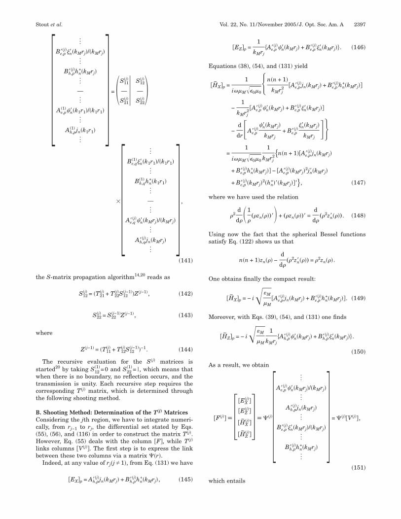
�141�
he S-matrix propagation algorithm14,20 reads as
S12�j� = �T21
�j� + T22�j�S12
�j−1��Z�j−1�, �142�
S22�j� = S22
�j−1�Z�j−1�, �143�
here
Z�j−1� = �T11�j� + T12
�j�S12�j−1��−1. �144�
The recursive evaluation for the S�j� matrices istarted20 by taking S12
�1�=0 and S22�1�=1, which means that
hen there is no boundary, no reflection occurs, and theransmission is unity. Each recursive step requires theorresponding T�j� matrix, which is determined throughhe following shooting method.
. Shooting Method: Determination of the T„j… Matricesonsidering the jth region, we have to integrate numeri-
ally, from rj−1 to rj, the differential set stated by Eqs.55), (56), and (116) in order to construct the matrix T�j�.owever, Eq. (55) deals with the column �F�, while T�j�
inks columns �V�j��. The first step is to express the linketween these two columns via a matrix ��r�.Indeed, at any value of rj�j�1�, from Eq. (131) we have
�EX�p = Ah,p��j�jn�kMrj� + Bh,p��j�hn+�kMrj�, �145�
�EZ�p =1
kMrj�Ae,p��j��n��kMrj� + Be,p��j��n��kMrj��. �146�
quations (38), (54), and (131) yield
�HX�p =1
i� M��0 0�n�n + 1�
kMrj2 �Ae,p��j�jn�kMrj� + Be,p��j�hn
+�kMrj��
−1
kMrj2 �Ae,p��j��n��kMrj� + Be,p��j��n��kMrj��
−d
dr�Ae,p��j�
�n��kMrj�
kMrj+ Be,p��j�
�n��kMrj�
kMrj
=1
i� M��0 0
1
kMrj2�n�n + 1��Ae,p��j�jn�kMrj�
+ Be,p��j�hn+�kMrj�� − �Ae,p��j��kMrj�2jn��kMrj�
+ Be,p��j��kMrj�2�hn+���kMrj���� , �147�
here we have used the relation
�2d
d��1
�„�zn���…�� + „�zn���…� =
d
d�„�2zn����…. �148�
sing now the fact that the spherical Bessel functionsatisfy Eq. (122) shows us that
n�n + 1�zn��� −d
d�„�2zn����… = �2zn���.
ne obtains finally the compact result:
�HX�p = − i� �M
M�Ae,p��j�jn�kMrj� + Be,p��j�hn
+�kMrj��. �149�
oreover, with Eqs. (39), (54), and (131) one finds
�HZ�p = − i� �M
M
1
kMrj�Ah,p��j��n��kMrj� + Bh,p��j��n��kMrj��.
�150�
s a result, we obtain
�F�j�� � ��EX
�j��
�EZ�j��
�HX�j��
�HZ�j��� � ��j��
]
Ae,p��j��n��kMrj�/�kMrj�
]
Ah,p��j�jn�kMrj�
]
Be,p��j��n��kMrj�/�kMrj�
]
Bh,p��j�hn+�kMrj�
]
� = ��j��V�j��,
�151�
hich entails
w
TsR
th4ptf
W��gvvw
w
C
Tt
COl(ttt
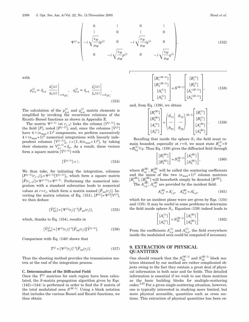
2398 J. Opt. Soc. Am. A/Vol. 22, No. 11 /November 2005 Stout et al.
��j� =�0 1 0 1
1 0 1 0
− i� �M
M/p�j� 0 − i� �M
M/q�j� 0
0 − i� �M
Mp�j� 0 − i� �M
Mq�j�� , �152�
a
m=
wa�
wat
Fi
9QOtjciacomt
ith
pp,q�j� � �p,q��n��z�
�n�z��
z=kMrj
, qp,q�j� � �p,q� �n��z�
�n�z��
z=kMrj
.
�153�
he calculation of the pp,q�j� and qp,q
�j� matrix elements isimplified by invoking the recurrence relations of theicatti–Bessel functions as shown in Appendix E.The matrix ��j−1� (at rj−1) links the column �V�j−1�� to
he field �F�, noted �F�j−1��, and, since the columns �V�j��ave 4� �nmax+1�2 components, we perform successively� �nmax+1�2 numerical integrations with linearly inde-endent columns �V�j−1��i, i� �1,4�nmax+1�2�, by takingheir elements as Vp,i
�j−1�=�pi. As a result, these vectorsorm a square matrix �V�j−1�� with
�V�j−1�� = 1. �154�
e thus take, for initiating the integration, columnsF�j−1��rj−1��i=��j−1��V�j−1��i, which form a square matrixF�rj−1��=��j−1�1=��j−1�. Performing the numerical inte-ration with a standard subroutine leads to numericalalues at r=rj, which form a matrix named �Fint�rj��. In-erting the matrix relation of Eq. (151), �F�j��=��j��V�j��,e then deduce
�Vint�j� � = ���j��rj��−1�Fint�rj��, �155�
hich, thanks to Eq. (154), results in
�Vint�j� � = ���j��rj��−1�Fint�rj���V�j−1��. �156�
omparison with Eq. (140) shows that
T�j� = ���j��rj��−1�Fint�rj��. �157�
hus the shooting method provides the transmission ma-rix at the end of the integration process.
. Determination of the Diffracted Fieldnce the T�j� matrices for each region have been calcu-
ated, the S-matrix propagation algorithm given by Eqs.142)–(144) is performed in order to find the S matrix ofhe total modulated area S�M−1�. Using a block notationhat includes the various Bessel and Ricatti functions, wehus obtain
��Be�
�M−1��
�Bh��M−1��
�Ae�1��
�Ah�1��
� = S�M−1���Be
�1��
�Bh�1��
�Ae��M−1��
�Ah��M−1��
� , �158�
nd, from Eq. (139), we obtain
��Be
�M��
�Bh�M��
�Ae�1��
�Ah�1��
� = �S11
—
S21��S12
—
S22�
�M−1���Be
�1��
�Bh�1��
�Ae�M��
�Ah�M��
� . �159�
Recalling that inside the sphere S1 the field must re-ain bounded, especially at r=0, we must state Beq
�1�=0Bhq
�1� ∀q. Thus Eq. (159) gives the diffracted field through
��Be�M��
�Bh�M�� = S12
�M−1���Ae�M��
�Ah�M�� , �160�
here Beq�M�, Bhq
�M� will be called the scattering coefficientsnd the union of the two �nmax+1�2 column matricesBe
�M��, �Bh�M�� will henceforth simply be denoted �B�M��.
The Ae,p�M�, Ae,p
�M� are provided by the incident field:
Ae,p�M� = Ae,p
i , Ah,p�M� = Ah,p
i , �161�
hich for an incident plane wave are given by Eqs. (134)nd (135). It may be useful in some problems to determinehe field inside sphere S1. Equation (159) indeed leads to
��Ae�1��
�Ah�1�� = S22
�M−1���Ae�M��
�Ah�M�� . �162�
rom the coefficients Ae,p�1� and Ah,p
�1� , the field everywherenside the modulated area could be computed if necessary.
. EXTRACTION OF PHYSICALUANTITIESne should remark that the S22
�M−1� and S12�M−1� block ma-
rices obtained by our method are rather complicated ob-ects owing to the fact they contain a great deal of physi-al information in both near and far fields. This detailednformation is essential if we wish to use these matricess the basic building blocks for multiple-scatteringodes.2,25 For a given single-scattering situation, however,ne is typically interested in studying more limited, butore physical accessible, quantities such as cross sec-
ions. This extraction of physical quantities has been ex-

ts
dicccu
fccam
s
atoo
it
titdf((a=ckWepl
ww
cF
wfit
s
w
Ta
dstcp
1Tttitrct
dpost
Stout et al. Vol. 22, No. 11 /November 2005 /J. Opt. Soc. Am. A 2399
ensively studied elsewhere,24–27 and we content our-elves here with a few illustrative formulas.
Physical quantities of interest can usually be obtainedirectly from analytical formulas of the coefficients of thencident and scattered fields. We recall that for a given in-ident field, with expansion coefficients placed in a �Ai�olumn vector and multiplied by suitable Bessel and Ri-atti functions to obtain the vector �A�M��, Eq. (160) allowss to obtain the scattering vector �B�M�� via
�B�M�� = S12�M−1��A�M��, �163�
rom which a vector �Bc�M�� containing only the scattering
oefficients can be derived. We shall define the Hermitianonjugate or adjoint vector �Bc�†, which takes the form ofrow matrix of the complex conjugates of the �Bc
�M�� ele-ents:
�Bc�M��† � �…,Beq
�M�,*,…�…,Bhq�M�,*,…�. �164�
The T-matrix, denoted here by t, familiar to the 3Dcattering community is defined by the equation
�Bc�M�� � t�Ai�, �165�
nd a comparison with Eqs. (141), (160), and (163) showshat the elements of t can be obtained from the elementsf S12
�M−1� through the multiplication by appropriate ratiosf Ricatti–Bessel functions.
With �Bc�M��, one can readily express the total scatter-
ng, extinction, and absorption cross sections, respec-ively, given by24,26
�s =1
kM2 �Bc�†�Bc�,
�e = Re� 1
kM2 �Bc�†�Ai� ,
�a = �e − �s. �166�
For a number of applications, however, total cross sec-ions provide too-crude information, and one is interestedn the angular distribution of the scattered radiation inhe far field. For such situations, it is frequently useful toefine an amplitude scattering matrix,2,6 F [not to be con-used with the F column used in propagation equations53) and (55) nor with the S matrix of Eqs. (141) and159)]. The scattering matrix is defined in the context ofn incident plane wave, which we express as Ei
E exp�ikM ·r��e��i+e��i�, where �i and �i are the spheri-al unit vectors associated with the incident wave vector,M. The scalar E has the dimensions of an electric field.e are in the habit of normalizing the polarization factors
� and e� such that �e��2+ �e��2=1, in which case E is sim-ly the electric field amplitude �Ei�=E. In the far-fieldimit, the scattered field at r→ will have the form
limr→
Es�r� = Eexp�ikr�
ikr�Es,�� + Es,���, �167�
here � and � are the spherical unit vectors associatedith the vector r. The scattered field factors E and E
s,� s,�an be calculated in terms of the 2�2 scattering matrix:
�Es,�
Es,�� = E
exp�ikr�
ikr�F�� F��
F�� F����e�
e�� , �168�
here each of the F elements is a function of the incidenteld direction �i, �i and the observation angle of the scat-ered field �, �. They can be calculated by defining the
cattering dyadic F¯
:
F¯ � 4��X*�r�,Z*�r��t�X�ki�
Z�ki� , �169�
here we call X and Z the phase-modified VSH24:
Xnm�r� � inXnm* �r�, Znm�r� � in−1Znm
* �r�. �170�
he F elements of Eq. (168) can then be readily expresseds
F�� � � · F¯
· �i, F�� � � · F¯
· �i, F�� � � · F¯
· �i,
F�� � � · F¯
· �i. �171�
The scattering matrix can subsequently be invoked toerive other angularly dependent physical quantitiesuch as the Stokes matrix.6,24,27 Here we simply remarkhat a quantity of frequent interest is the differentialross section d� /d, which in our notation can be com-uted from6,24,27
d�
d��,�;�i,�i� = lim
r→
r2�Es�r��2
E2 =�Es,��2 + �Es,��2
k2
=�F�� e� + F�� e��2 + �F�� e� + F��e��2
k2 .
�172�
0. CONCLUSIONhis achieves the detailed presentation of the differential
heory of light diffraction by a 3D object. Although theheory makes use of the basis of vector spherical harmon-cs, which is much more complicated to manipulate thanhe Fourier basis used in Cartesian coordinates, the finalesult looks quite simple in the sense that it is not moreomplicated than analyzing crossed gratings,20 for whichhe propagation equations are quite similar.
The current theory can also be extended to treat theiffraction from anisotropic materials. A forthcoming pa-er will present numerical results concerning prolate andblate spheroids and will include comparisons with re-ults given by approximate methods in view of studyingheir domain of validity.

t
e
AIrft=e
r
U
w
a
a
iay
Sc
∀�
Ta
AEED
P(
Utfi
Ta
(
U
2400 J. Opt. Soc. Am. A/Vol. 22, No. 11 /November 2005 Stout et al.
The authors thank Sophie Stout for helpful contribu-ions.
Corresponding author B. Stout can be reached by-mail at [email protected]
PPENDIX A: CALCULATION OF �N,0
n the case of an axisymmetric object, in the modulatedegion the permittivity ��r ,�� is a piecewise constantunction with step discontinuities. With c=cos �, ��r ,�� isransformed into ��r ,c�, and Eq. (34) reads as �n,0
2�!−11 ��r ,c�Pn
0�c�dc, where Pn0 are the normalized Leg-
ndre polynomials:
Pn0�cos �� = �2n + 1
4��1/2
Pn0�cos ��. �A1�
We can evaluate this integral by invoking the recur-ence relation
�n + 1�Pn0�c� =
d
dcPn+1
0 �c� − cd
dcPn
0�c�. �A2�
sing the relation
d
dc„cPn
0�c�… = cd
dcPn
0�c� + Pn0�c�, �A3�
e find
cd
dcPn
0�c� =d
dc„cPn
0�c�… − Pn0�c�, �A4�
nd the recurrence relation becomes
Pn0�c� =
1
n
d
dcPn+1
0 �c� −1
n
d
dc„cPn
0�c�…. �A5�
We have then
c2
c1
Pn0�c�dc =
1
n
c2
c1 d
dcPn+1
0 �c�dc −1
n
c2
c1 d
dc„cPn
0�c�…dc,
�A6�
nd the piecewise integral is then
c2
c1
Pn0�c�dc =
1
n�Pn+1
0 �c1� − Pn+10 �c2�� +
1
n�c2Pn
0�c2�
− c1Pn0�c1��. �A7�
An example of the determination of the �n,0 coefficientss illustrated on a spheroid with half large and small axesand b, respectively; Oz is the symmetry axis, and, in the
Oz plane, its Cartesian equation is
z2
a2 +y2
b2 = 1. �A8�
ince z=r cos � and y=r sin �, this equation in sphericaloordinates reads as
r��� =ab
� 2 2 2 2. �A9�
a + �b − a �cos �
Inversing this relation leads to
��r� = arccos�a
r� r2 − b2
a2 − b2� �A10�
r� �b ,a�; Eq. (A10) defines a value �1�r�, with �1�r��0,� /2�. Defining �2�r�=�−�1�r�, we have
��r,�� = �1 if � � �0,�1�r�� � ��2�r�,��,
��r,�� = �M if � � ��1�r�,�2�r��. �A11�
he limits c1 and c2 that appear in Eq. (A7) are cos �1�r�nd cos �2�r�.
PPENDIX B: VANISHING OF SOMELEMENTS OF THE Q� MATRIXxpanding D and E on the basis of VSH, the equation=�0�E gives
�n�,m�
�DYn�m�Yn�m� + DXn�m�Xn�m� + DZn�m�Zn�m��
= �0��r,�,����,
�EY� Y� + EX� X� + EZ� Z� �.
�B1�
erforming an ordinary scalar product of both sides of Eq.B1) with Ynm
* , we obtain
Ynm* · �
n�,m�
�DYn�m�Yn�m� + DXn�m�Xn�m� + DZn�m�Zn�m��
= �0��r,�,��Ynm* · �
�, �EY� Y� + EX� X� + EZ� Z� �.
�B2�
sing the fact as one can see from Eqs. (7), (16), and (17)hat Ynm
* ·Xn�m�=Ynm* ·Zn�m�=Ynm
* ·X� =Ynm* ·Z� =0, we
nd
�n�,m�
DYnmYnm* · Yn�m� = �0��r,�,���
�, EY� Ynm
* · Y� .
�B3�
his equation establishes a linear relation between DYnmnd EY� only; thus Q�YX and Q�YZ must be null.Now, performing a scalar product on both sides of Eq.
B1) with Xnm* , we find that
Xnm* · �
n�,m�
�DYn�m�Yn�m� + DXn�m�Xn�m� + DZn�m�Zn�m��
= �0��r,�,��Xnm* · �
�, �EY� Y� + EX� X� + EZ� Z� �.
�B4�
sing the fact that X* ·Y =X* ·Y =0, we obtain
nm n�m� nm �
Ia
SQ
s
AVInotorv
wnc
w
dawVY
f
1U
PG
2It
i
U
IG
Stout et al. Vol. 22, No. 11 /November 2005 /J. Opt. Soc. Am. A 2401
1
�0�
n�,m�
�DXn�m�Xnm* · Xn�m� + DZn�m�Xnm
* · Zn�m��
= ��r,�,��Xnm* · �
�, �EX� X� + EZ� Z� �. �B5�
ntegrating over the solid angles , we obtain, taking intoccount Eq. (11),
DXnm = �0��,
0
4�
d��r,�,��Xnm* · �EX� X� + EZ� Z� �.
�B6�
ince DXnm does not depend on EY� , we deduce that�XY=0.A similar calculation starting from multiplying both
ides of Eq. (B1) by Znm* leads to Q�ZY=0.
PPENDIX C: TWO RELATIONS BETWEENECTOR SPHERICAL HARMONICS
n order to derive two relations between VSHs that areecessary to construct the theory, it is useful to invoke an-ther set of VSHs, denoted Yn,n+1
m , Yn,nm , and Yn,n−1
m , as in-roduced by quantum-mechanic theoreticians who workedn the angular-momentum coupling formalism.23 We firstecall the definition of the Cartesian spherical unitectors23:
X1 = −1
�2�x + iy�, X0 = z, X−1 =
1
�2�x − iy�,
�C1�
here x, y, z are the unit vectors of the Cartesian coordi-ate system. Making use of the Clebsch–Gordanoefficients,23 we then define the new set of VSHs as
Yn,lm = �
=−1
1
�l,m − ;1, �n,m�Yl,m− X , �C2�
ith l=n−1, n, n+1.Using the conversion from spherical to Cartesian coor-
inates and the expressions of our Ynm, Xnm, Znm VSHs inspherical coordinate system of Eqs. (7), (16), and (17),e can painstakingly verify that our Ynm, Xnm, and ZnmSHs can be expressed in terms of the Yn,n+1
m , Yn,n+1m ,
n,n+1m spherical harmonics via the relations
Xnm =Yn,n
m
i, �C3�
Znm = � n + 1
2n + 1�1/2
Yn,n−1m + � n
2n + 1�1/2
Yn,n+1m , �C4�
Ynm = � n
2n + 1�1/2
Yn,n−1m − � n + 1
2n + 1�1/2
Yn,n+1m . �C5�
With the above equations in place, we first calculate theollowing two products.
. X�� ·Xnm*
sing Eq. (C3), we find
X� · Xnm* = Y�,�
· �Yn,nm �*. �C6�
utting Eq. (C2) in Eq. (C6) and calculating the Clebsch–ordan coefficients lead us to
X� · Xnm* = � 1
n�n + 1���� + 1� 1/2
��1
2��n + m + 1��n − m��� + + 1��� − ��1/2
�Y�, +1Yn,m+1* + m Y� Ynm
*
+1
2��n + m��n − m + 1�
��� + ��� − + 1��1/2Y�, −1Yn,m−1* . �C7�
. X�� ·Znm*
n order to calculate this scalar product, we use the facthat X� ·Ynm
* =0. Thus Eq. (C5) gives
� n + 1
2n + 1�1/2
X� · Yn,n+1m,* = � n
2n + 1�1/2
X� · Yn,n−1m,* ,
�C8�
.e.,
X� · Yn,n+1m,* = � n
n + 1�1/2
X� · Yn,n−1m,* . �C9�
sing Eq. (C4), we then obtain
X� · Znm* = � n + 1
2n + 1�1/2
X� · Yn,n−1m,*
+ � n
2n + 1�1/2
X� · Yn,n+1m,*
= �2n + 1
n + 1�1/2
X� · Yn,n−1m,*
= − i�2n + 1
n + 1�1/2
Y�,� · Yn,n−1
m,* . �C10�
nserting Eq. (C2) and the expression of the Clebsch–ordan coefficients into Eq. (C10) leads to
X� · Znm* = i� 1
n�n + 1���� + 1�
2n + 1
2n − 1�1/2
��−Y�, −1Yn−1,m−1
*
2
���n + m��n + m − 1��� + ��� − + 1��1/2

ACTtoofs
cfs
M
(−E
A
F
2402 J. Opt. Soc. Am. A/Vol. 22, No. 11 /November 2005 Stout et al.
+ ��n2 − m2��1/2Y�, Yn−1,m* +
Y�, +1Yn−1,m+1*
2
���n − m��n − m − 1��� − ��� + + 1��1/2 .
�C11�
PPENDIX D: USE OF THE GAUNTOEFFICIENTSheoreticians working on the coupling of angular momen-um in quantum mechanics have introduced the conceptsf Gaunt coefficients and Wigner 3J coefficients.23,28 Withur definitions, the normalized Gaunt coefficients, a, ariserom solid-angle integration of the product of three scalar
23
pherical harmonics : tcomparison with Eq. (77) shows that
itssl
bt�
a����, ��,��, �,�n,m�� � 0
2� 0
�
Y�� ���,��Y� ��,��
�Ynm��,��sin �d�d�. �D1�
These coefficients can be rapidly calculated through re-ursion relations.29 They naturally appear if, startingrom Eq. (71), we expand in it the ��r ,� ,�� function astated in Eq. (3):
�n�m�
�DTYn�m�Yn�m� + DTXn�m�Xn�m� + DTZn�m�Zn�m��
= �0 ���, �
��,
��� �Y�� ��ETY� Y� + ETX� X� + ETZ� Z� �.
�D2�
ultiplying both sides by Ynm* �� ,�� and integrating over
he angular variables �, �, we obtain
1
�0DTYnm = �
��, ���,
��� �ETY� /Y�� ���,��Y� ��,�� · Ynm
* ��,��sin �d�d�
= ���, �
��,
��� �ETY� �− 1�m/
Y�� ���,��Y� ��,�� · Yn,−m��,��sin �d�d�
= ���, �
��,
��� �ETY� �− 1�m/
Y�� ���,��Y� ��,��Yn,−m��,��sin �d�d�
= ���, �
��,
��� �ETY� �− 1�ma����, ��,��, �,�n,− m��. �D3�
A useful property of Gaunt coefficients defined in Eq.D1) is that they are null except if �=m− and ��� ��n�� ,n+��. Thus the summation over � is eliminated, andq. (D3) reduces to
DTYnm = �0 ���=�n−��
n+�
��=0
N
� =−�
�
�− 1�ma����,m − �,
��, �,�n,− m�����,m− ETY� . �D4�
�YYnm,� = �− 1�m ���=�n−��
n+�
a����,m − �,��, �,�n,
− m�����,m− �r�, �D5�
n which the calculation of ���,m− �r� involves computinghe integrals stated in Eq. (6), which implies integratingingle spherical harmonics multiplied by piecewise con-tant functions, a task that can readily be performed ana-ytically as described in Appendix A.
We now can derive similar expressions for the otherlocks. Multiplying both sides of Eq. (71) by Xnm
* �� ,��, in-egrating over the angular variables �, �, and expanding
as stated by Eq. (3), we obtainDTXnm = �0 ���, �
��,
��� �ETX� Y�� ���,��X� ��,�� · Xnm* ��,��sin �d�d�
+ ���, �
��,
��� �ETZ� Y�� ���,��Z� ��,�� · Xnm* ��,��sin �d�d�. �D6�
rom Eq. (C7) in Appendix C we thus obtain

F
c
wl
AFW�
Tu
mt
Stout et al. Vol. 22, No. 11 /November 2005 /J. Opt. Soc. Am. A 2403
�XXnm,� = � 1
n�n + 1���� + 1� 1/2
�− 1�−m ���=�n−��
n+�
���,m− � �−1
2��n + m + 1��n − m��� + + 1��� − ��1/2a����,m − �,��, + 1�,�n,
− m − 1�� + a����,m − �,��, �,�n,− m�� −1
2��n + m��n − m + 1��� + ��� − + 1��1/2a����,m − �,��, − 1�,�n,− m
+ 1�� . �D7�
rom Eq. (C11) in Appendix C, we obtain
�XZnm,� =i
2� 1
n�n + 1���� + 1�
2n + 1
2n − 1�1/2
�− 1�m ���=�n−1−��
n+�−1
���,m− � ˆ− ��n + m��n + m − 1��� + ��� − + 1��1/2a����,m
− �,��, �,�n − 1,− m + 1�� + 2 ��n2 − m2��1/2a����,m − �,��, �,�n − 1,− m�� + ��n − m��n − m − 1��� − ��� +
+ 1��1/2a����,m − �,��, + 1�,�n − 1,− m − 1��‰ . �D8�
wr
somv
R
1
An alternative exists to determine the Gaunt coeffi-ients. Introducing the Wigner 3J coefficients
� n1 n2 n3
m1 m2 m3� ,
hich are given by standard subroutines, we can calcu-ate the normalized Gaunt coefficients from
a����, ��,��, �,�n,m�� = � �2�� + 1��2� + 1��2n + 1�
4� 1/2
���� � n
0 0 0���� � n
� m� .
PPENDIX E: RICATTI–BESSELUNCTIONSe recall the definition of the Ricatti–Bessel functions
n�z� and �n�z�:
�n�z� � zjn�z�, �n�z� � zhn+�z�. �E1�
heir derivatives �n��z� and �n��z� can be readily calculatedsing the Bessel function recursion relations:
�n��z� =�n + 1�
z�n�z� − �n+1�z�,
�n��z� =�n + 1�
z�n�z� − �n+1�z�. �E2�
We note, for example, the elements of the p�j� and q�j�
atrices of Eq. (152) are simply the logarithmic deriva-ives of the Ricatti–Bessel functions:
pp,q�j� � �pq�n�kMrj� � ��pq
�n��z�
�n�z��
z=kMrj
,
qp,q�j� � �pq�n�kMrj� � ��pq
�n��z�
�n�z��
z=kMrj
, �E3�
hich can be rapidly and reliably calculated1 from recur-ence relations derived from Eqs. (E2),
�n−1�z� =n
z−
1
�n�z� + n/z,
or
�n�z� =1
n/z − �n−1�z�−
n
z, �E4�
o that Ricatti–Bessel functions simplify the initializationf the shooting method. Of course, the partition of theodulated area should be done in such a way that no
alue of rj coincides with a zero of a Ricatti �n�z� function.
EFERENCES AND NOTES1. C. F. Bohren and D. R. Huffman, Absorption and Scattering
of Light by Small Particles (Wiley-Interscience, 1983).2. M. I. Mischenko L. D. Travis, and A. A. Lacis, Scattering,
Absorption, and Emission of Light by Small Particles(Cambridge U. Press, 2002).
3. L. Lorenz, “Lysbevaegelsen i og uden for en af planeLysbølger belyst Kulge,” Vidensk. Selk. Skr. 6, 1–62 (1890).
4. L. Lorenz, “Sur la lumière réfléchie et réfractée par unesphère transparente,” Librairie Lehmann et Stage,Oeuvres scientifique de L. Lorenz, revues et annotées parH. Valentiner, 1898 (transl. of Ref. 3).
5. G. Mie, “Beiträge zur Optik Trüber Medien speziellkolloidaler Metallosungen,” Ann. Phys. 25, 377–452 (1908).
6. L. Tsang, J. A. Kong, and R. T. Shin, Theory of MicrowaveRemote Sensing (Wiley, 1985).
7. L. Tsang, J. A. Kong, and K.-H. Ding, Scattering ofElectromagnetic Waves, Theories and Applications (Wiley,2000).
8. L. Tsang, J. A. Kong, K.-H. Ding, and C. O. Ao, Scatteringof Electromagnetic Waves, Numerical Simulations (Wiley,2001).
9. L. Tsang and J. A. Kong, Scattering of ElectromagneticWaves, Advanced Topics (Wiley, 2001).
0. In the community of grating theoreticians, as well as in theone of waveguides, this matrix is called the S matrix or

1
1
1
1
1
1
1
1
1
2
2
22
2
2
2
2
2
2
2404 J. Opt. Soc. Am. A/Vol. 22, No. 11 /November 2005 Stout et al.
scattering matrix. It is essentially the S12 block of theS�M−1� matrix appearing later on in Eq. (158); see also Eqs.(163) and (165).
1. W. C. Chew, Waves and Fields in Inhomogeneous Media,IEEE Press Series on Electromagnetic Waves (IEEE, 1994).
2. P. C. Waterman, “Matrix methods in potential theory andelectromagnetic scattering,” J. Appl. Phys. 50, 4550–4566(1979).
3. M. Bagieu and D. Maystre, “Waterman and Rayleighmethods for diffraction grating problems: extension of theconvergence domain,” J. Opt. Soc. Am. A 15, 1566–1576(1998).
4. L. Li, “Formulation and comparison of two recursive matrixalgorithms for modeling layered diffraction gratings,” J.Opt. Soc. Am. A 13, 1024–1035 (1996).
5. E. Popov and M. Nevière, “Grating theory: new equationsin Fourier space leading to fast converging results for TMpolarization,” J. Opt. Soc. Am. A 17, 1773–1784(2000).
6. E. Popov and M. Nevière, “Maxwell equations in Fourierspace: fast converging formulation for diffraction byarbitrary shaped, periodic, anisotropic media,” J. Opt. Soc.Am. A 18, 2886–2894 (2001).
7. L. Li, “Use of Fourier series in the analysis ofdiscontinuous periodic structures,” J. Opt. Soc. Am. A 13,1870–1876 (1996).
8. E. Popov, M. Nevière, and N. Bonod, “Factorization ofproducts of discontinuous functions applied to
Fourier–Bessel basis,” J. Opt. Soc. Am. A 21, 46–51 (2004).9. N. Bonod, E. Popov, and M. Neviere, “Differential theory ofdiffraction by finite cylindrical objects,” J. Opt. Soc. Am. A22, 481–490 (2005).
0. M. Nevière and E. Popov, Light Propagation in PeriodicMedia: Diffraction Theory and Design (Marcel Dekker,2003).
1. C. Cohen-Tannoudji, Photons & Atomes—Introduction àl’électrodynamique quantique (InterEdition/ Editions duCNRS, 1987).
2. J. D. Jackson, Classical Electrodynamics (Wiley, 1965).3. A. R. Edmonds, Angular Momentum in Quantum
Mechanics (Princeton U. Press, 1960).4. B. Stout, J.-C. Auger, and J. Lafait, “Individual and
aggregate scattering matrices and cross-sections:conservation laws and reciprocity,” J. Mod. Opt. 48,2105–2128 (2001).
5. B. Stout, J. C. Auger, and J. Lafait, “A transfer matrixapproach to local field calculations in multiple scatteringproblems,” J. Mod. Opt. 49, 2129–2152 (2002).
6. D. W. Mackowski, “Calculation of total cross sections ofmultiple-sphere clusters,” J. Opt. Soc. Am. A 11, 2851–2861(1994).
7. D. W. Mackowski, and M. I. Mishchenko, “Calculation ofthe T matrix and the scattering matrix for ensembles ofspheres,” J. Opt. Soc. Am. A 13, 2266–2278 (1996).
8. J. A. Gaunt, “On the triplets of Helium,” Philos. Trans. R.Soc. London, Ser. A 228, 151–196 (1929).
9. Y. L. Xu, “Fast evaluation of the Gaunt coefficients,” Math.
Comput. 65, 1601–1612 (1996).