!

Ligand Field Theory

Frank Neese!Max-Planck Institut für Chemische EnergiekonversionStifstr. 34-36D-45470 Mülheim an der Ruhr!frank.Neese@cec.mpg.de

3rd Penn State Bioinorganic Workshop May/June 2014

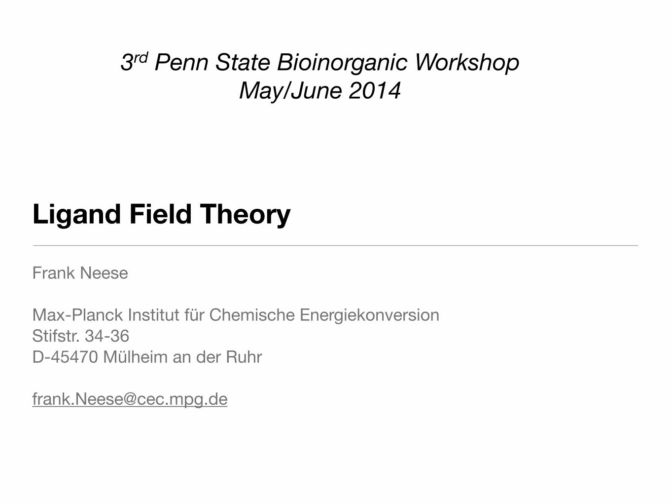
Theory in Chemistry

Observable Facts

(Experiments)ChemicalLanguage

Phenomenological Models

SemiempiricalTheories

MolecularRelativistic

SchrödingerEquation

NonrelativisticQuantum

Mechanics

Hartree-FockTheory

CorrelatedAb InitioMethods

DensityFunctional

Theory

NUMBERSUNDERSTANDING

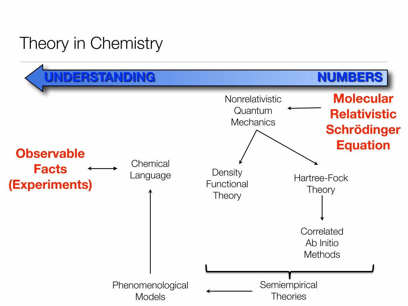
What is Ligand Field Theory ?

★ Ligand Field Theory is: ‣ A semi-empirical theory that applies to a CLASS of substances (transition

metal complexes).‣ A LANGUAGE in which a vast number of experimental facts can be

rationalized and discussed.‣ A MODEL that applies only to a restricted part of reality.!

★ Ligand Field Theory is NOT: ‣ An ab initio theory that lets one predict the properties of a compound ‚from

scratch‘‣ A physically rigorous treatment of transition metal electronic structure

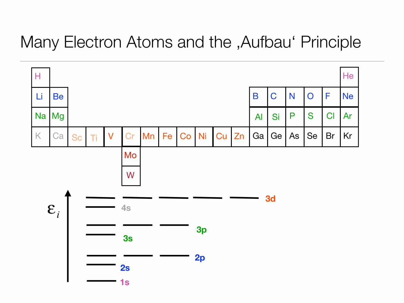
Many Electron Atoms and the ‚Aufbau‘ Principle

1s2s

2p

3s3p

4s3d

Sc Ti V Cr Mn Fe Co Ni Cu ZnK Ca

H He

Li Be B C N O F Ne

Ar

Kr

Al Si P S Cl

Ga Ge As Se Br

Na Mg

Mo

W

States of Atoms and Molecules

★ Atoms and Molecule exist in STATES

★ ORBITALS can NEVER be observed in many electron systems !!!

★ A STATE of an atom or molecule may be characterized by four criteria:

1. The distribution of the electrons among the available orbitals (the electron CONFIGURATION) (A set of occupation numbers)

2. The overall SYMMETRY of the STATE (Γ Quantum Number)

3. The TOTAL SPIN of the STATE (S-Quantum Number)

4. The PROJECTION of the Spin onto the Z-axis (MS Quantum Number)

|nSkMΓMΓ>

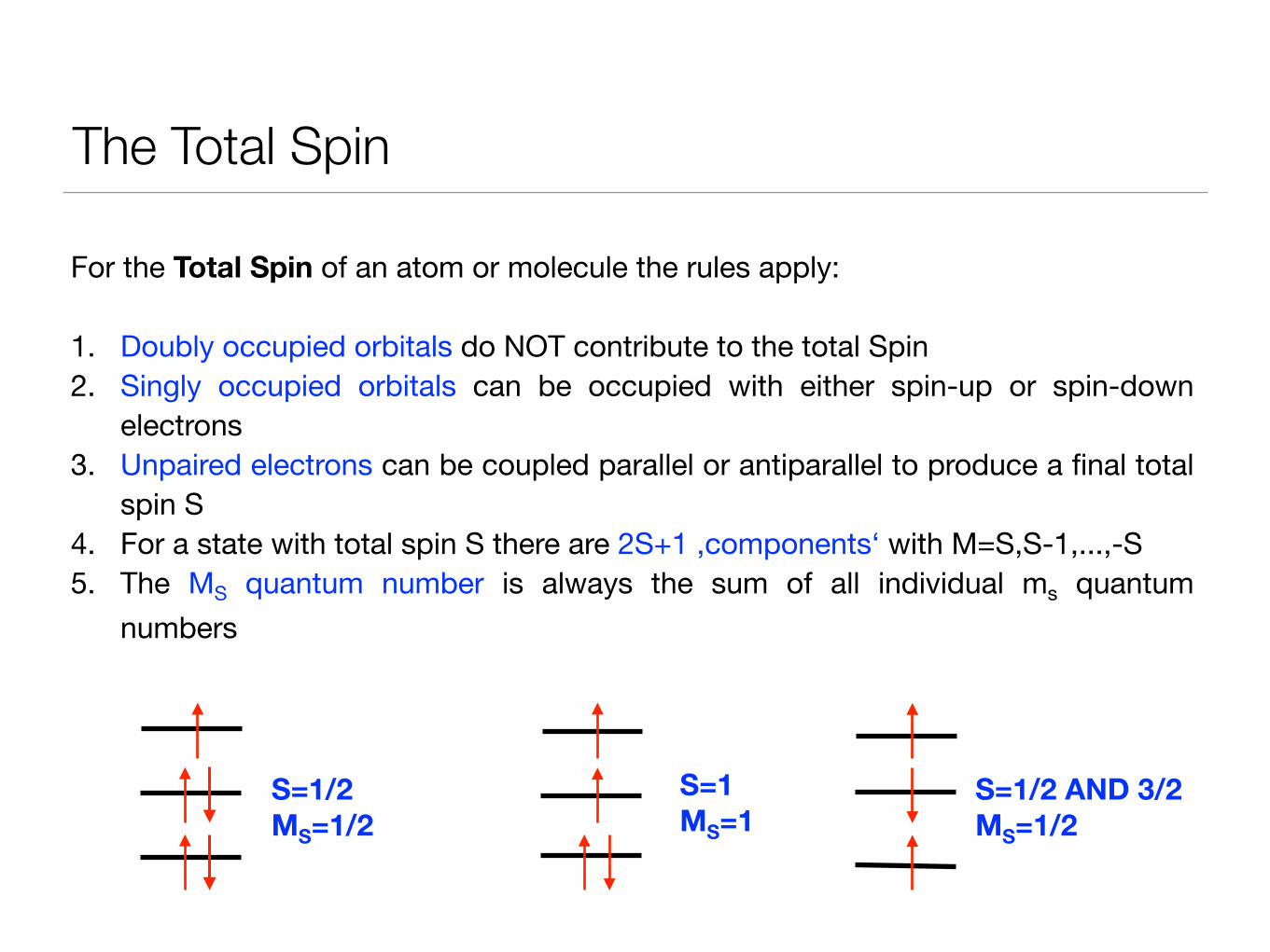
The Total Spin

For the Total Spin of an atom or molecule the rules apply:!1. Doubly occupied orbitals do NOT contribute to the total Spin2. Singly occupied orbitals can be occupied with either spin-up or spin-down

electrons3. Unpaired electrons can be coupled parallel or antiparallel to produce a final total

spin S4. For a state with total spin S there are 2S+1 ‚components‘ with M=S,S-1,...,-S5. The MS quantum number is always the sum of all individual ms quantum

numbers

S=1/2 MS=1/2

S=1 MS=1

S=1/2 AND 3/2 MS=1/2

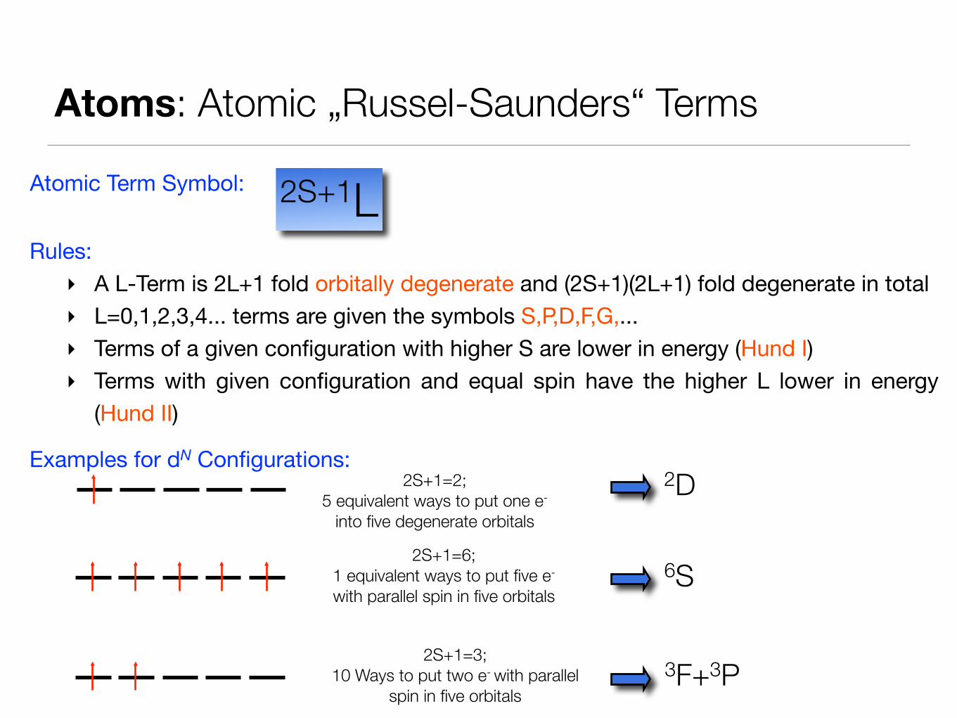
Atoms: Atomic „Russel-Saunders“ Terms

Rules:‣ A L-Term is 2L+1 fold orbitally degenerate and (2S+1)(2L+1) fold degenerate in total‣ L=0,1,2,3,4... terms are given the symbols S,P,D,F,G,...‣ Terms of a given configuration with higher S are lower in energy (Hund I)‣ Terms with given configuration and equal spin have the higher L lower in energy

(Hund II)

Atomic Term Symbol: 2S+1L

Examples for dN Configurations:2S+1=2;

5 equivalent ways to put one e-

into five degenerate orbitals

2D

2S+1=6; 1 equivalent ways to put five e-

with parallel spin in five orbitals6S

2S+1=3; 10 Ways to put two e- with parallel

spin in five orbitals3F+3P

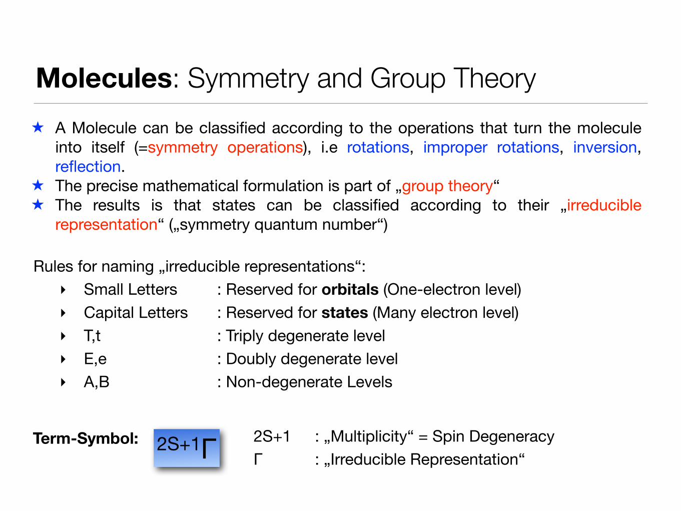
Molecules: Symmetry and Group Theory

Rules for naming „irreducible representations“:‣ Small Letters : Reserved for orbitals (One-electron level)‣ Capital Letters : Reserved for states (Many electron level)‣ T,t : Triply degenerate level‣ E,e : Doubly degenerate level‣ A,B : Non-degenerate Levels

Term-Symbol: 2S+1Γ 2S+1 : „Multiplicity“ = Spin DegeneracyΓ : „Irreducible Representation“

★ A Molecule can be classified according to the operations that turn the molecule into itself (=symmetry operations), i.e rotations, improper rotations, inversion, reflection.

★ The precise mathematical formulation is part of „group theory“★ The results is that states can be classified according to their „irreducible

representation“ („symmetry quantum number“)

Principles of Ligand Field Theory

Example:

R-L| Mδ- δ+

Strong Attraction

NegativePositive

Electrostatic Potential

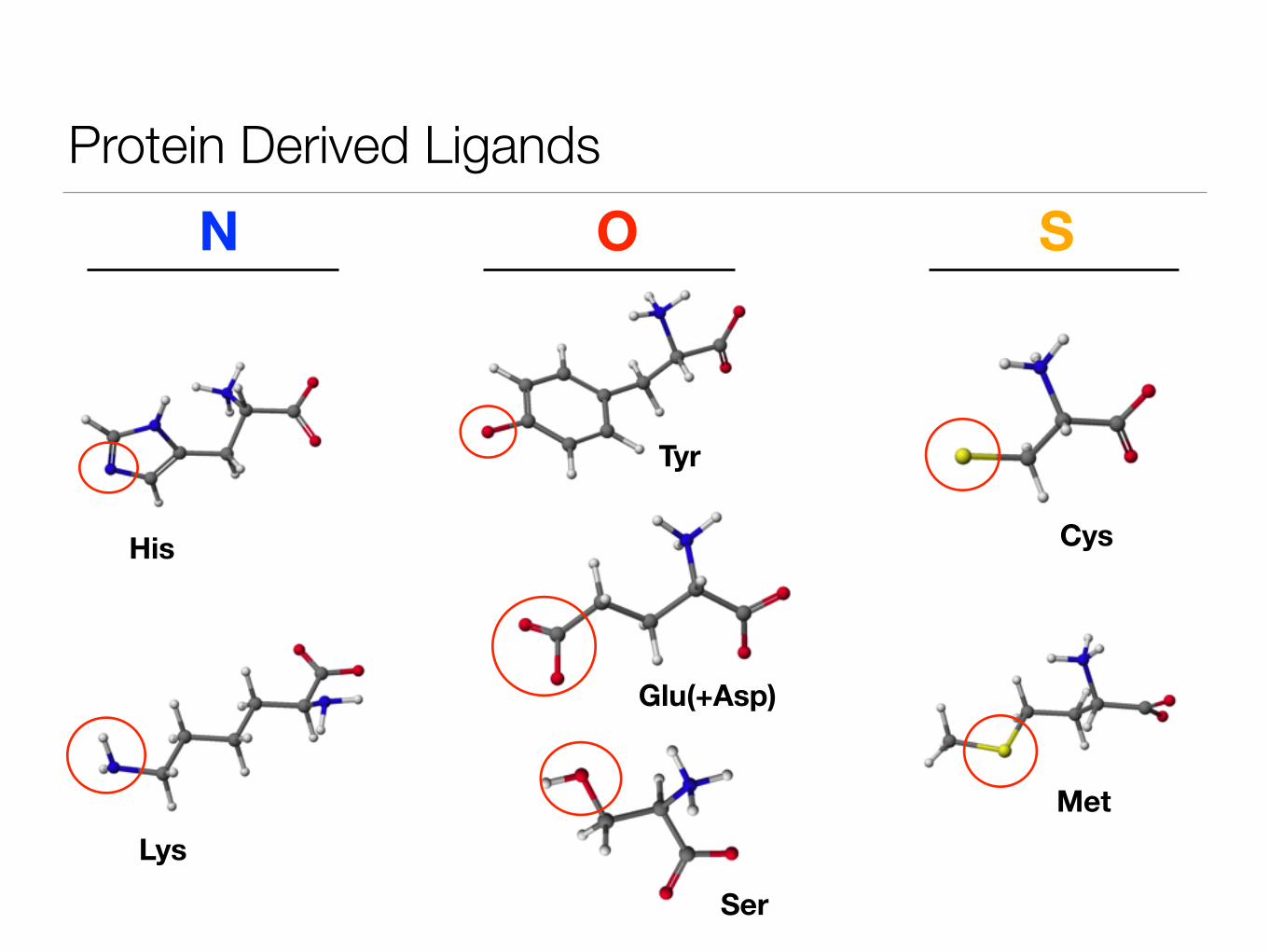
Protein Derived LigandsN O S

His

Lys

Tyr

Glu(+Asp)

Ser

Cys

Met

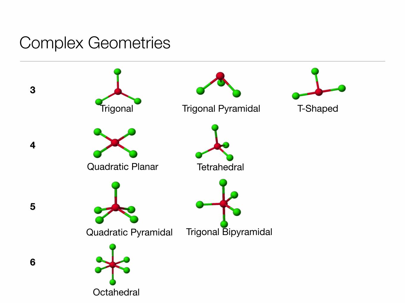
Complex Geometries

3

4

5

6

Trigonal Trigonal Pyramidal T-Shaped

Quadratic Planar Tetrahedral

Quadratic Pyramidal Trigonal Bipyramidal

Octahedral

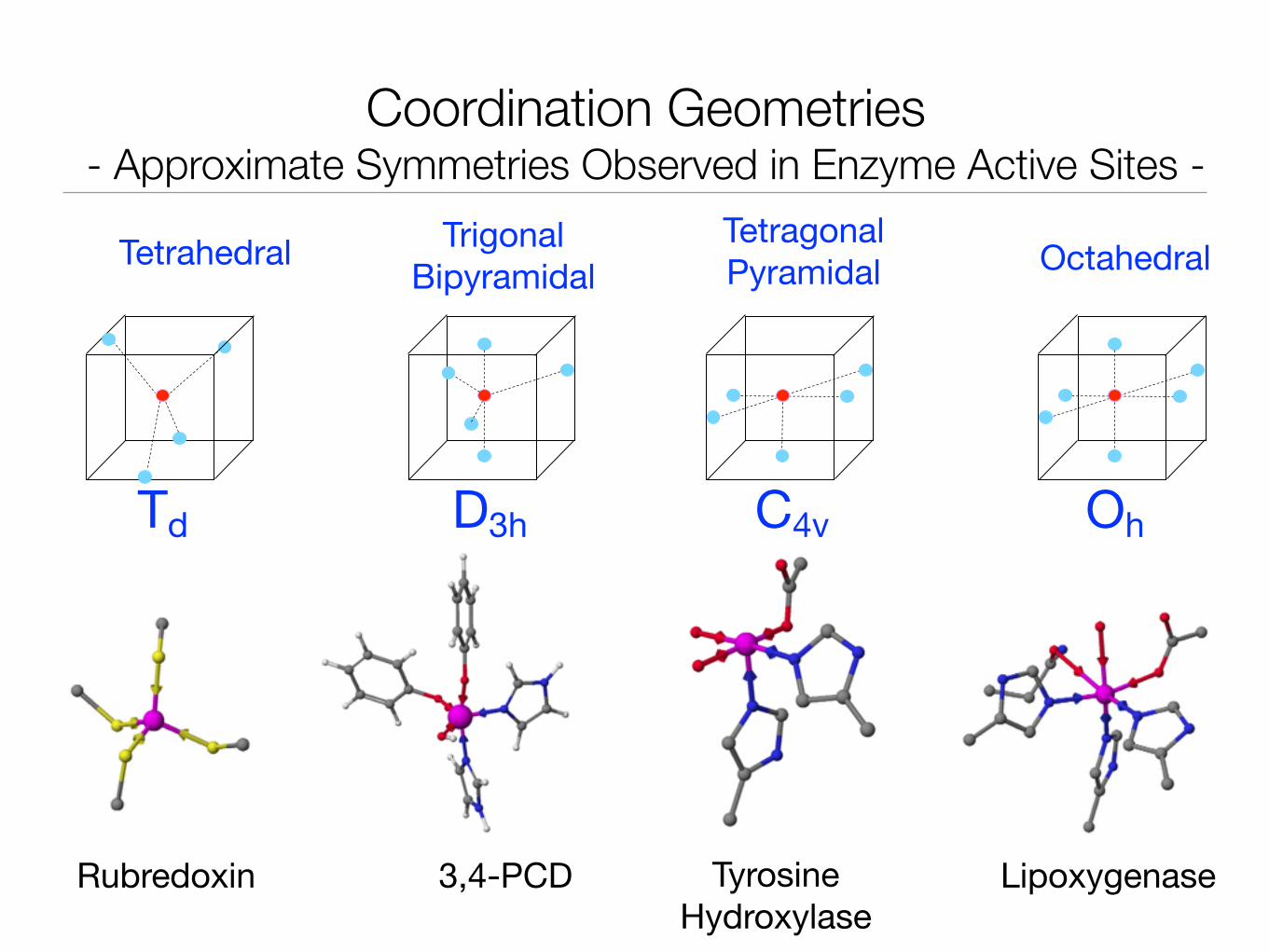
Rubredoxin 3,4-PCD TyrosineHydroxylase

Lipoxygenase

Tetrahedral TrigonalBipyramidal

TetragonalPyramidal Octahedral

Coordination Geometries- Approximate Symmetries Observed in Enzyme Active Sites -

Td D3h C4v Oh

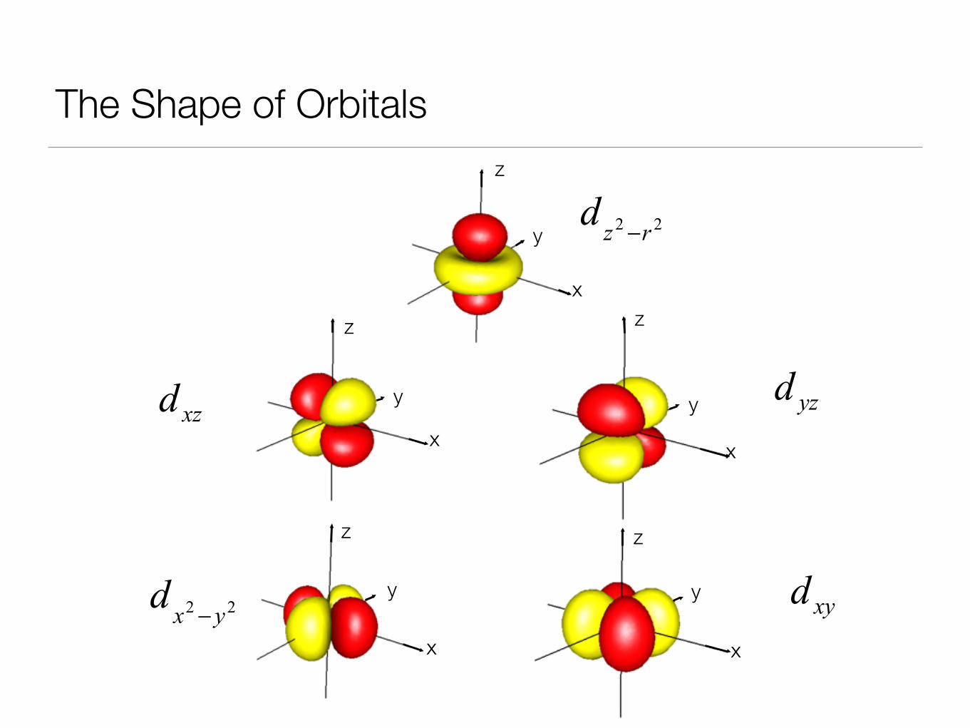
The Shape of Orbitals

x

x

xx

x

y

y

yy

y

z

zz

z z

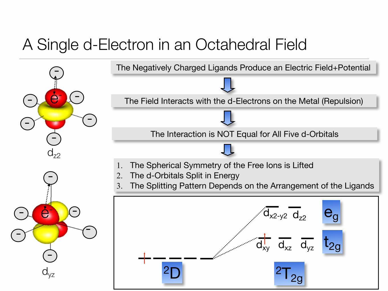
A Single d-Electron in an Octahedral FieldThe Negatively Charged Ligands Produce an Electric Field+Potential

The Field Interacts with the d-Electrons on the Metal (Repulsion)

The Interaction is NOT Equal for All Five d-Orbitals

1. The Spherical Symmetry of the Free Ions is Lifted2. The d-Orbitals Split in Energy3. The Splitting Pattern Depends on the Arrangement of the Ligands

2D

dxy dxz dyz

dx2-y2 dz2

t2g

eg

2T2g

dz2

dyz

--

--

--

-

---

--

e-

e-

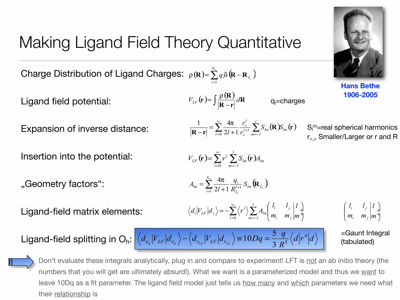
Making Ligand Field Theory QuantitativeCharge Distribution of Ligand Charges:

Ligand field potential:

Expansion of inverse distance:

Insertion into the potential:

„Geometry factors“:

Ligand-field matrix elements:

qi=charges

Slm=real spherical harmonics

r<,> Smaller/Larger or r and R

=Gaunt Integral (tabulated)Ligand-field splitting in Oh:

Don‘t evaluate these integrals analytically, plug in and compare to experiment! LFT is not an ab initio theory (the numbers that you will get are ultimately absurd!). What we want is a parameterized model and thus we want to leave 10Dq as a fit parameter. The ligand field model just tells us how many and which parameters we need what their relationship is

Hans Bethe 1906-2005

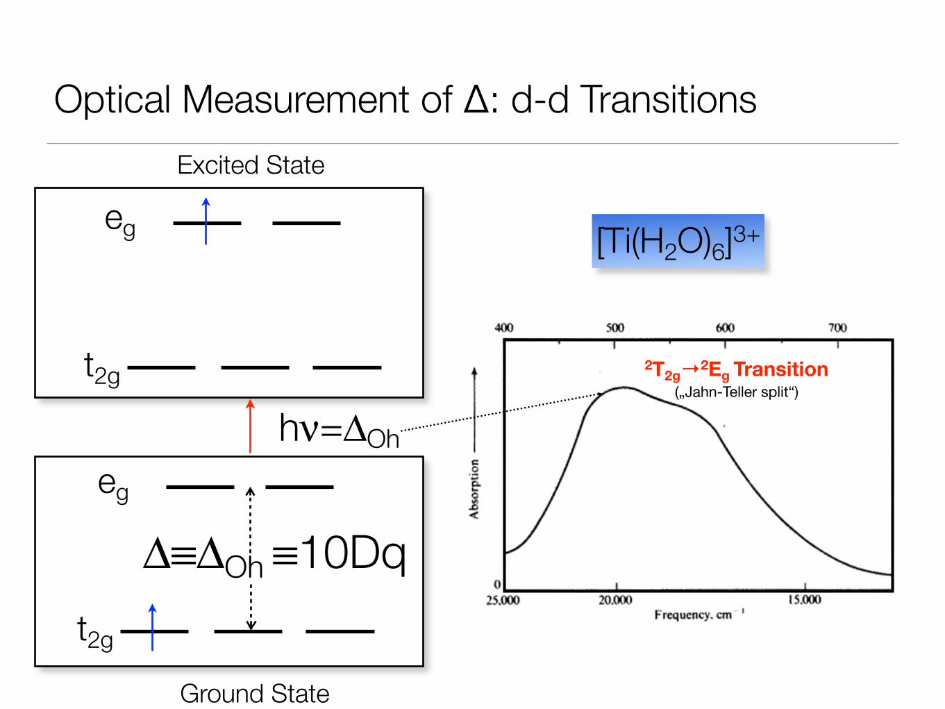
Optical Measurement of Δ: d-d Transitions

[Ti(H2O)6]3+

2T2g→2Eg Transition („Jahn-Teller split“)

eg

t2g

Δ≡ΔOh ≡10Dq

hν=ΔOh

eg

t2g

Ground State

Excited State

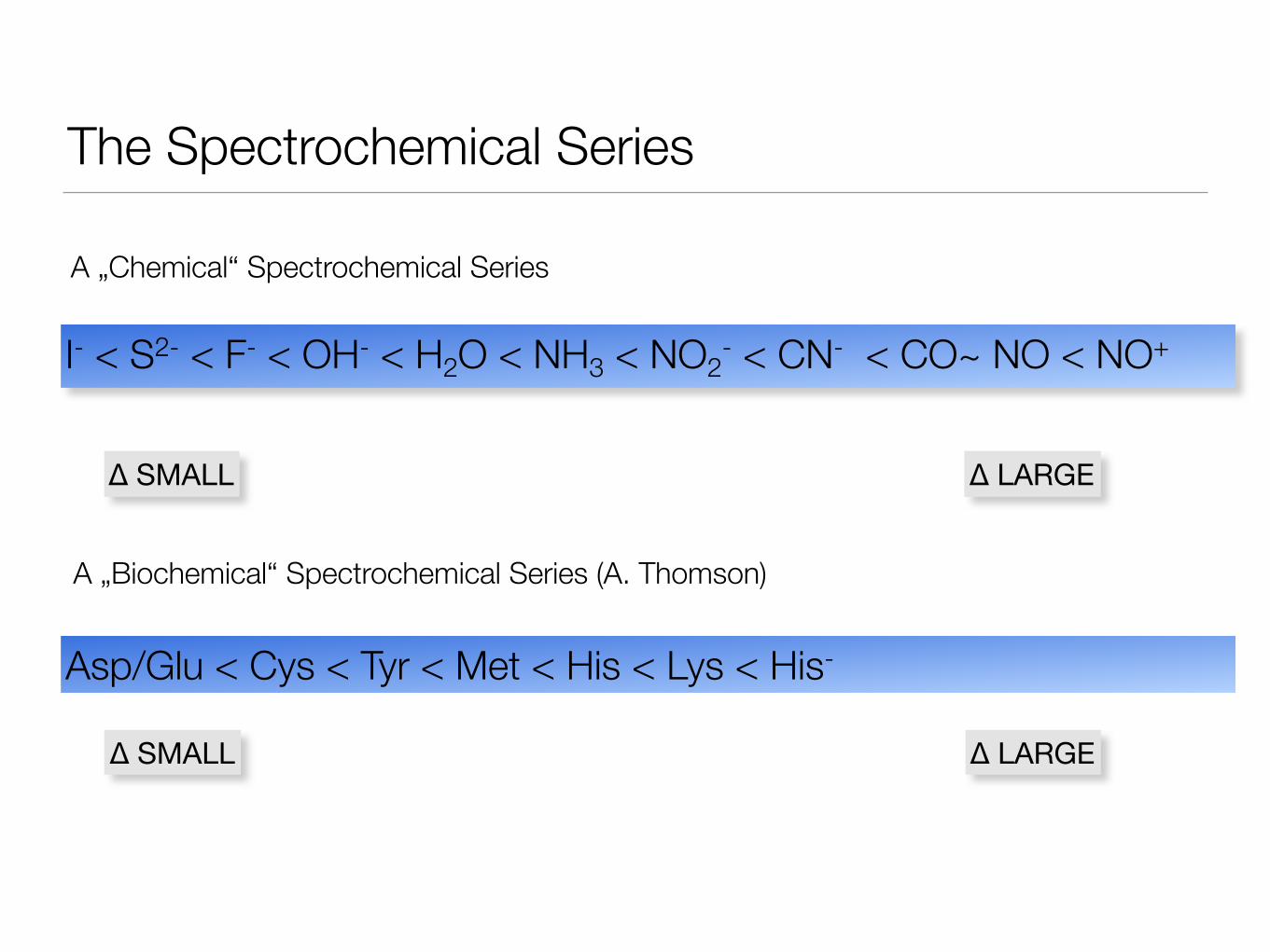
The Spectrochemical Series

A „Chemical“ Spectrochemical Series

A „Biochemical“ Spectrochemical Series (A. Thomson)

Δ LARGEΔ SMALL

Δ LARGEΔ SMALL

I- < S2- < F- < OH- < H2O < NH3 < NO2- < CN- < CO~ NO < NO+

Asp/Glu < Cys < Tyr < Met < His < Lys < His-

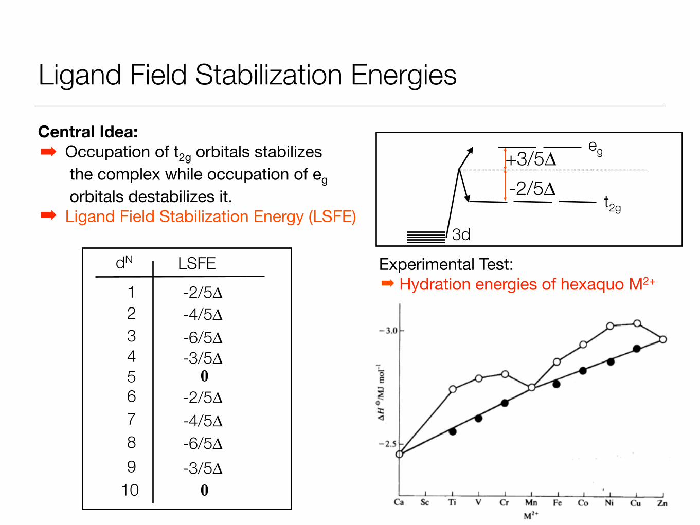
Ligand Field Stabilization Energies

Central Idea: ➡ Occupation of t2g orbitals stabilizes

the complex while occupation of eg orbitals destabilizes it.

➡ Ligand Field Stabilization Energy (LSFE)

Experimental Test:➡ Hydration energies of hexaquo M2+

t2g

eg

-2/5Δ+3/5Δ

dN LSFE123456789

10

0

0

-2/5Δ-4/5Δ-6/5Δ-3/5Δ

-2/5Δ-4/5Δ-6/5Δ-3/5Δ

3d

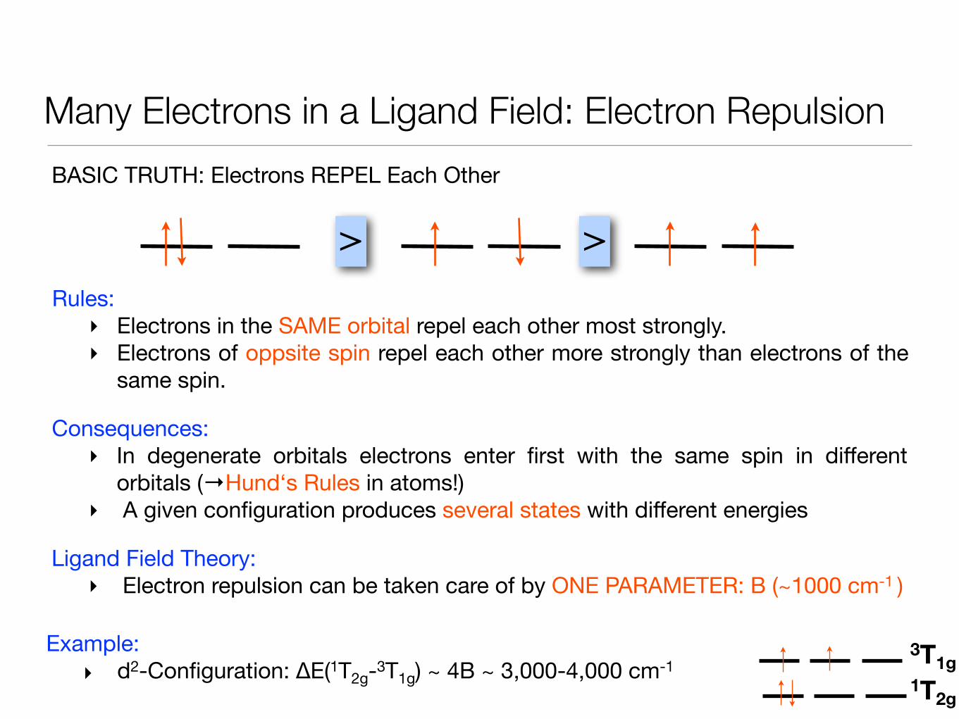
Many Electrons in a Ligand Field: Electron RepulsionBASIC TRUTH: Electrons REPEL Each Other

> >Rules:

‣ Electrons in the SAME orbital repel each other most strongly.‣ Electrons of oppsite spin repel each other more strongly than electrons of the

same spin.

Consequences:‣ In degenerate orbitals electrons enter first with the same spin in different

orbitals (→Hund‘s Rules in atoms!)‣ A given configuration produces several states with different energies

Ligand Field Theory:‣ Electron repulsion can be taken care of by ONE PARAMETER: B (~1000 cm-1 )

Example: ‣ d2-Configuration: ΔE(1T2g-3T1g) ~ 4B ~ 3,000-4,000 cm-1

1T2g

3T1g

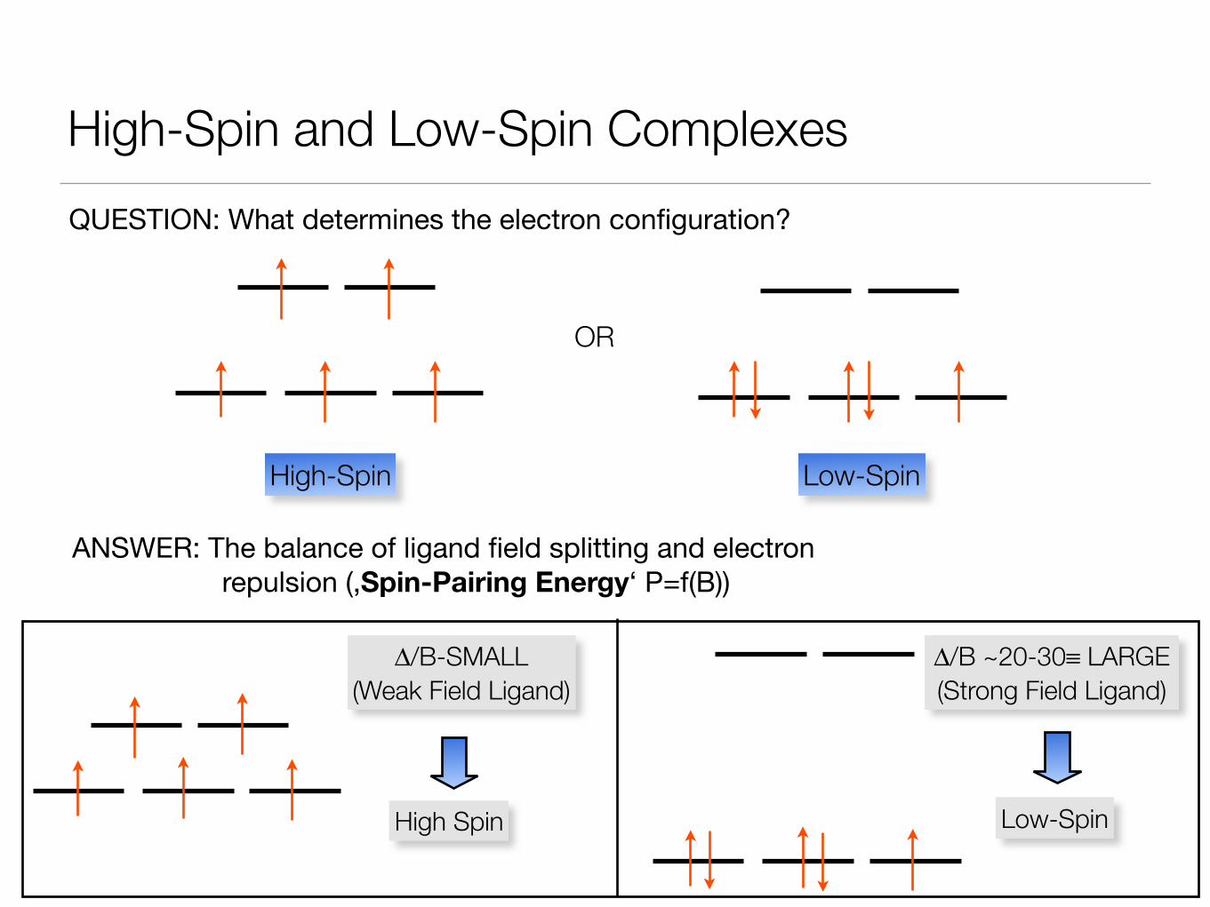
High-Spin and Low-Spin ComplexesQUESTION: What determines the electron configuration?

OR

High-Spin Low-Spin

ANSWER: The balance of ligand field splitting and electron repulsion (‚Spin-Pairing Energy‘ P=f(B))

Δ/B-SMALL (Weak Field Ligand)

High Spin

Δ/B ~20-30≡ LARGE (Strong Field Ligand)

Low-Spin

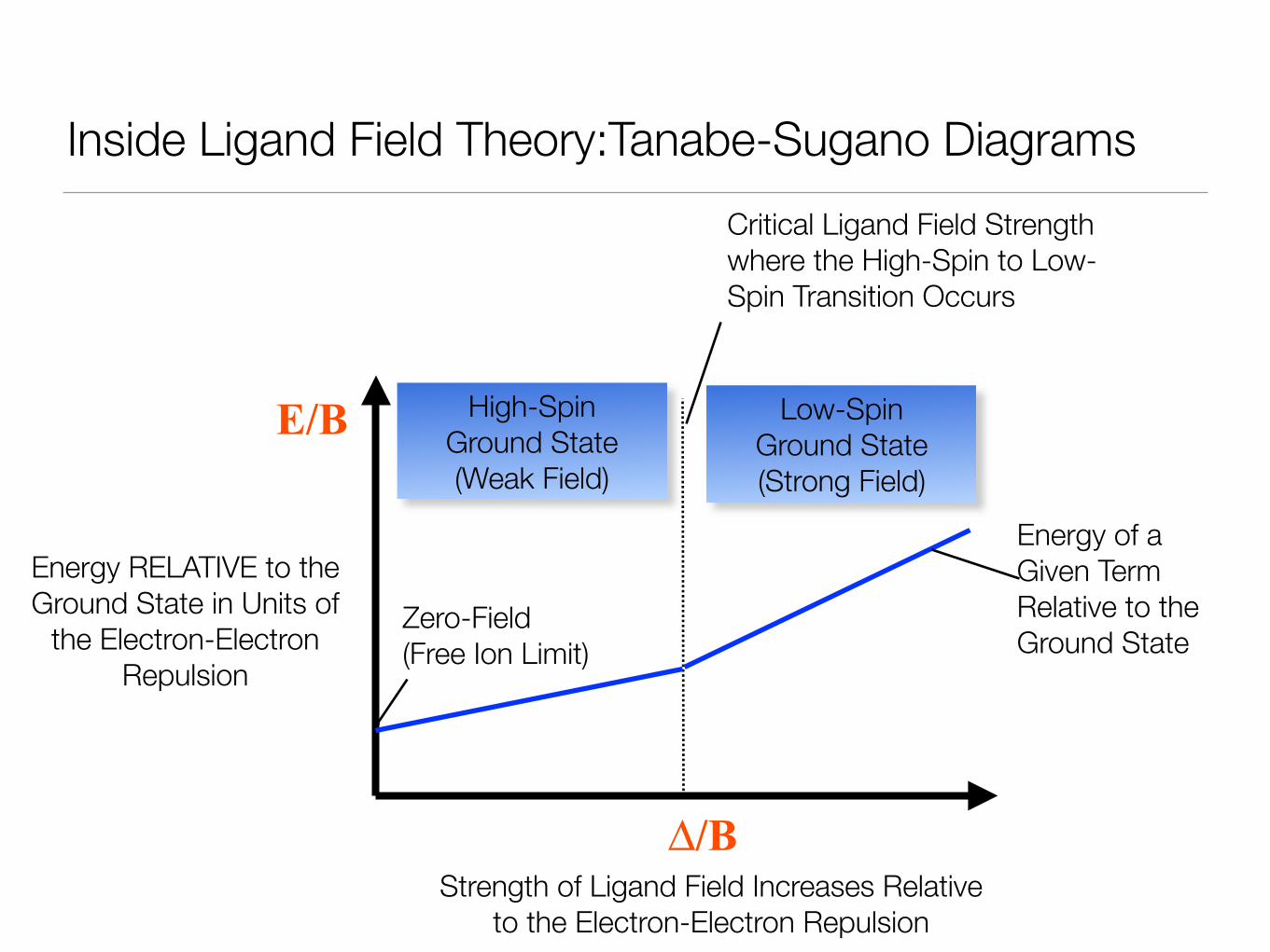
Inside Ligand Field Theory:Tanabe-Sugano Diagrams

Δ/BStrength of Ligand Field Increases Relative

to the Electron-Electron Repulsion

E/B

Energy RELATIVE to the Ground State in Units of

the Electron-Electron Repulsion

Critical Ligand Field Strength where the High-Spin to Low-Spin Transition Occurs

High-SpinGround State(Weak Field)

Low-SpinGround State (Strong Field)

Zero-Field (Free Ion Limit)

Energy of a Given Term Relative to the Ground State

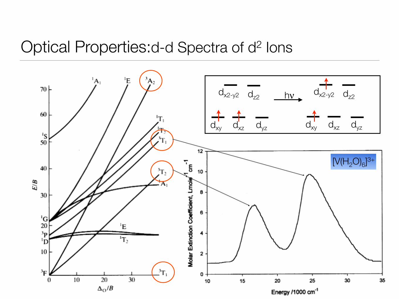
Optical Properties:d-d Spectra of d2 Ions

dxy dxz dyz

dx2-y2 dz2

dxy dxz dyz

dx2-y2 dz2hν

[V(H2O)6]3+

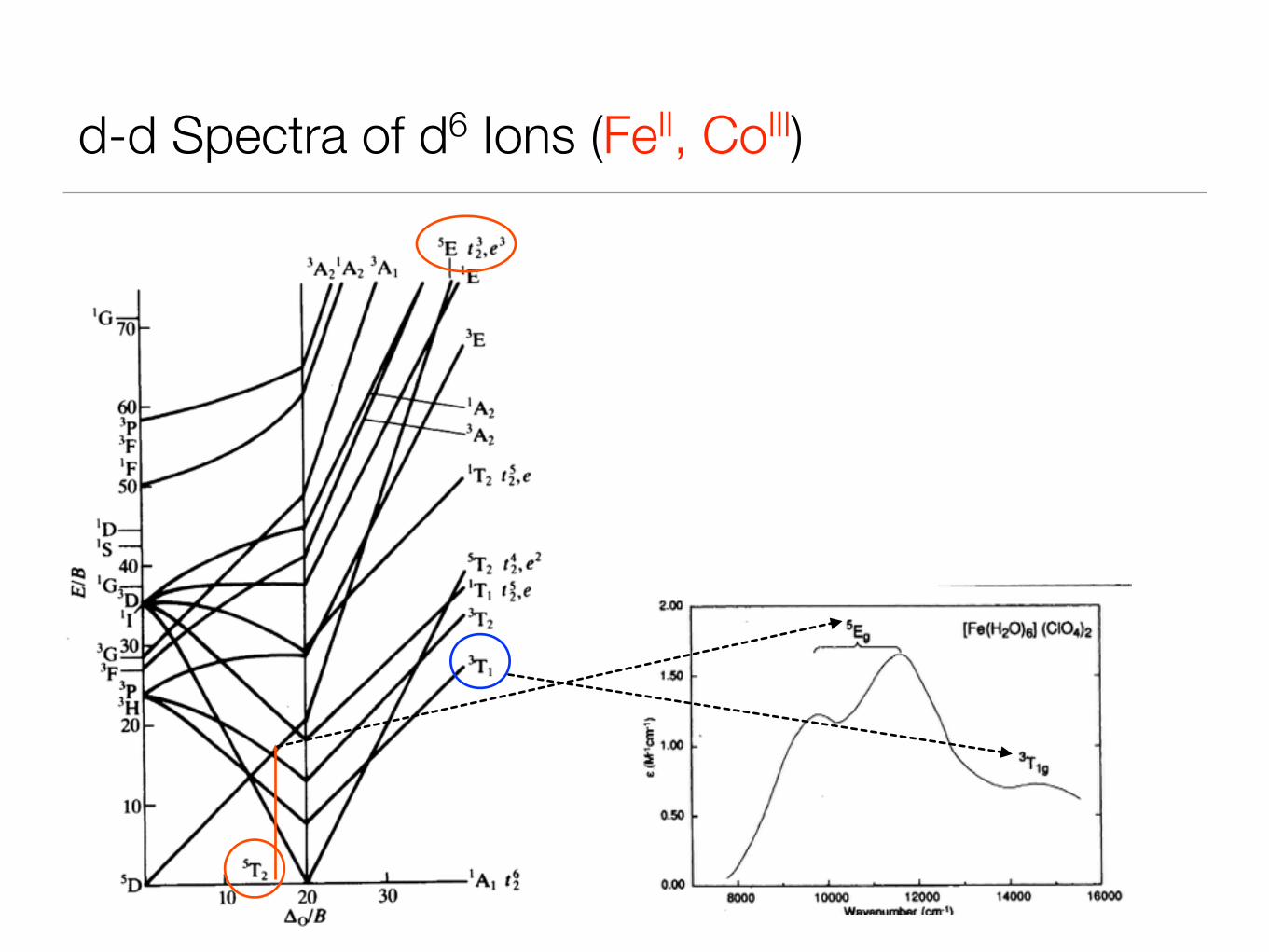
d-d Spectra of d6 Ions (FeII, CoIII)

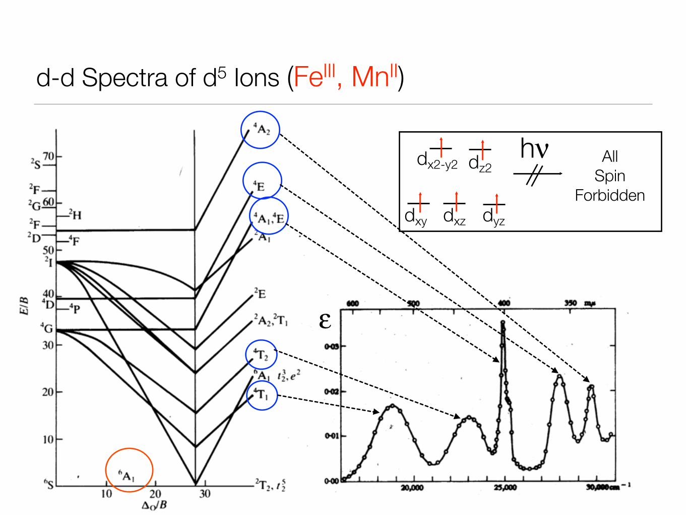
d-d Spectra of d5 Ions (FeIII, MnII)

ε

dxy dxz dyz

dx2-y2 dz2hν All

Spin Forbidden

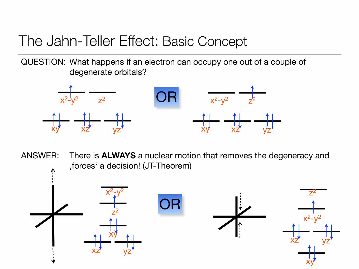
The Jahn-Teller Effect: Basic Concept

xy

xz yz

x2-y2

z2

QUESTION: What happens if an electron can occupy one out of a couple of degenerate orbitals?

xy xz yz

x2-y2 z2OR

ANSWER: There is ALWAYS a nuclear motion that removes the degeneracy and ‚forces‘ a decision! (JT-Theorem)

xy xz yz

x2-y2 z2

xy

xz yz

x2-y2

z2

OR

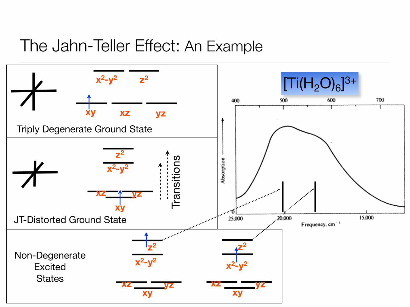
The Jahn-Teller Effect: An Example

[Ti(H2O)6]3+

xy xz yz

x2-y2 z2

xyxz yz

x2-y2z2

Triply Degenerate Ground State

JT-Distorted Ground State

xyxz yz

x2-y2

z2

xyxz yz

x2-y2

z2Non-Degenerate

Excited States

Tran

sitio

ns

xy xy xy

xy

xy

xzxz

xz

xzxz

yzyz

yz

yzyz

x2-y2 x2-y2 x2-y2

x2-y2

x2-y2

z2

z2

z2

z2

z2

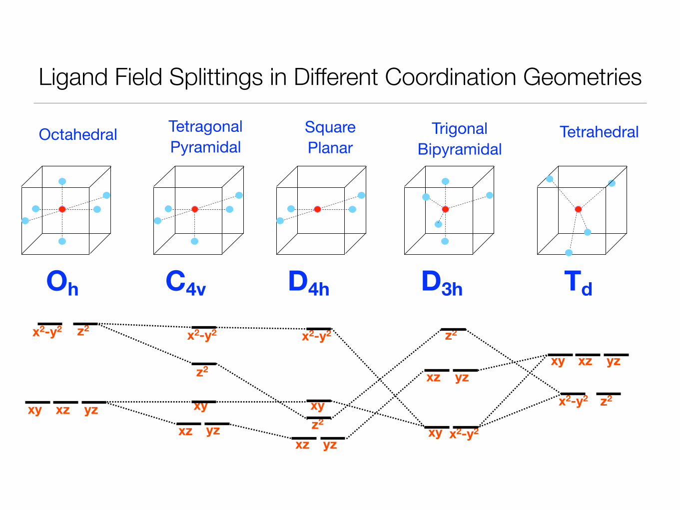
Ligand Field Splittings in Different Coordination Geometries

TdD3hC4vOh D4h

TetrahedralTrigonalBipyramidal

TetragonalPyramidal

Octahedral SquarePlanar

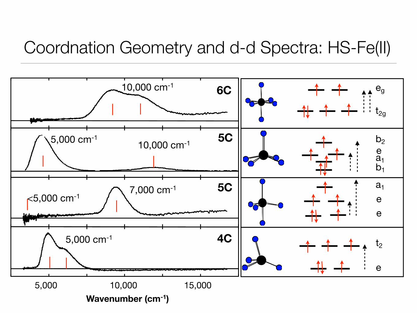
Coordnation Geometry and d-d Spectra: HS-Fe(II)

5C

5C

4C

6C10,000 cm-1

10,000 cm-15,000 cm-1

7,000 cm-1<5,000 cm-1

5,000 cm-1

5,000 10,000 15,000Wavenumber (cm-1)

eg

t2g

a1

ee

a1eb1

b2

t2

e

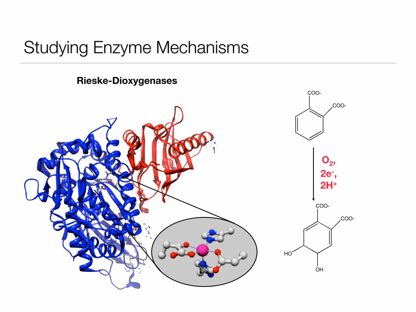
Studying Enzyme Mechanisms

O2, 2e-, 2H+

Rieske-Dioxygenases

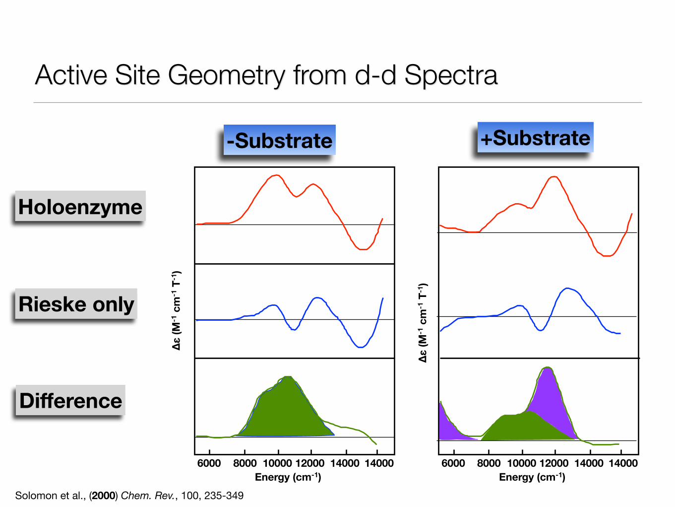
Active Site Geometry from d-d Spectra

Holoenzyme

Rieske only

Difference

-Substrate +Substrate

6000 8000 10000 12000 14000 14000Energy (cm-1)

6000 8000 10000 12000 14000 14000Energy (cm-1)

Δε (M

-1 c

m-1

T-1

)

Δε (M

-1 c

m-1

T-1

)

Solomon et al., (2000) Chem. Rev., 100, 235-349

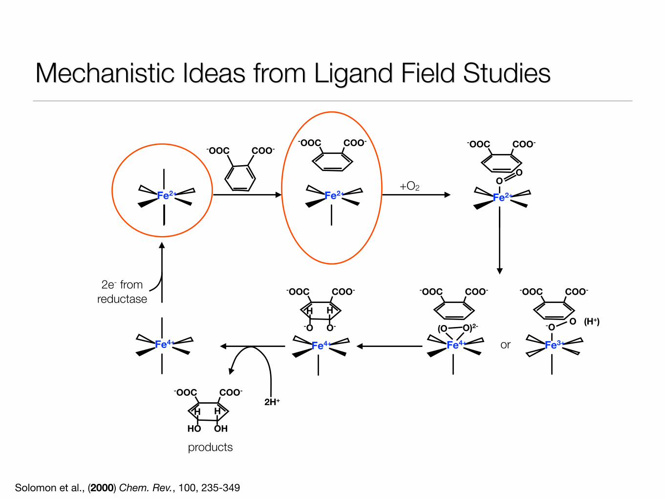
Mechanistic Ideas from Ligand Field Studies

Solomon et al., (2000) Chem. Rev., 100, 235-349

Fe2+ Fe2+ Fe2+

Fe4+ Fe3+Fe4+Fe4+

COO--OOCCOO--OOC COO--OOC

OO

COO--OOC

(O O)2-

COO--OOC

-O O (H+)

COO--OOC

H H-O O-

2H+COO--OOC

H H

HO OH

2e- from reductase

products

or

+O2

Beyond Ligand Field Theory

„Personally, I do not believe much of the electrostatic romantics, many of my collegues talked about“

(C.K. Jörgensen, 1966 Recent Progress in Ligand Field Theory)

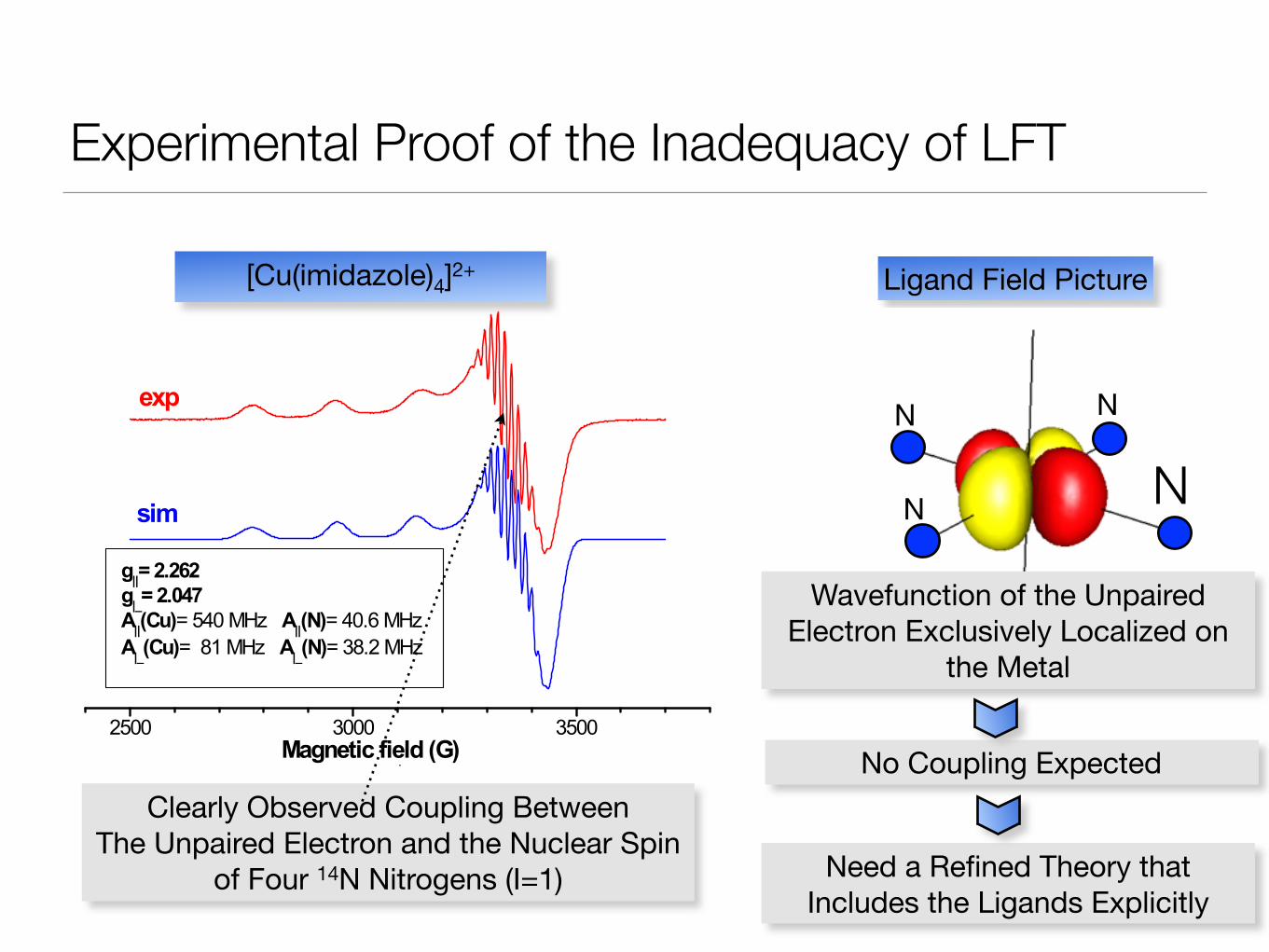
Experimental Proof of the Inadequacy of LFT

[Cu(imidazole)4]2+ Ligand Field Picture

Clearly Observed Coupling BetweenThe Unpaired Electron and the Nuclear Spin

of Four 14N Nitrogens (I=1)

Wavefunction of the Unpaired Electron Exclusively Localized on

the Metal

No Coupling Expected

Need a Refined Theory that Includes the Ligands Explicitly

N N

NN

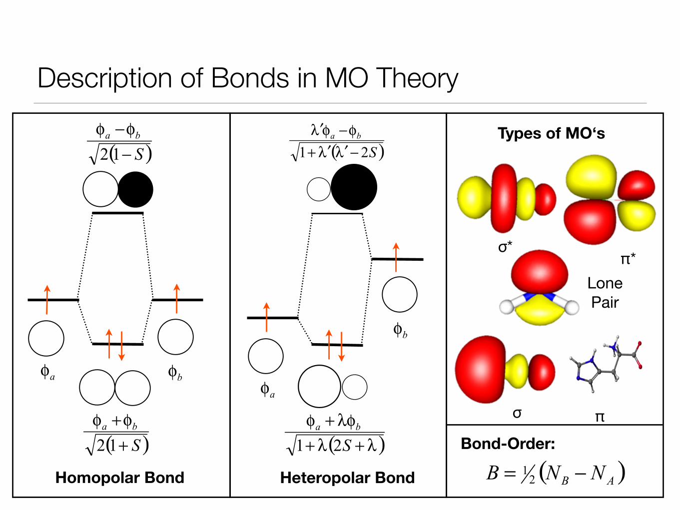
Description of Bonds in MO Theory

Homopolar Bond Heteropolar Bond

Bond-Order:

Types of MO‘s

σ*π*

σ π

Lone Pair

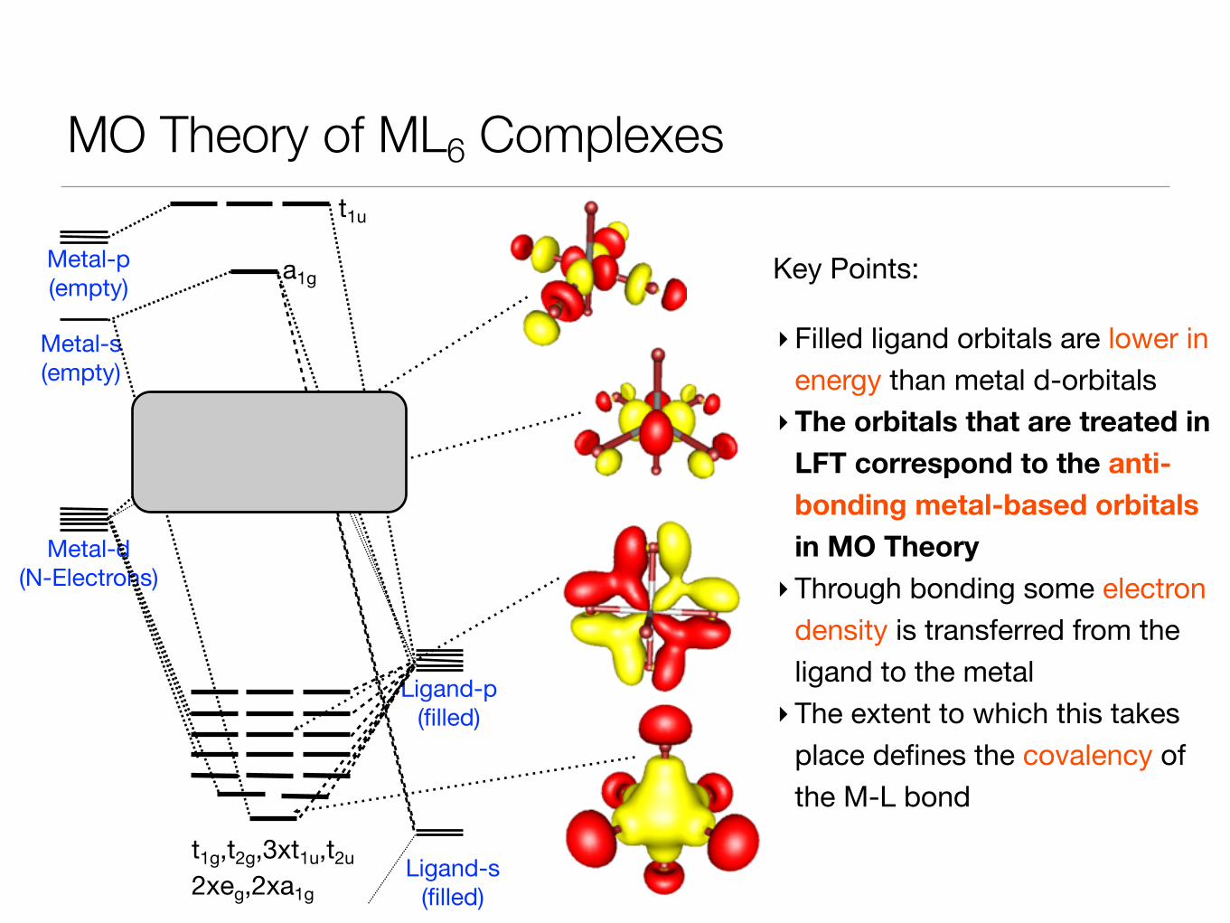
MO Theory of ML6 Complexes

Key Points:!‣Filled ligand orbitals are lower in

energy than metal d-orbitals ‣The orbitals that are treated in

LFT correspond to the anti-bonding metal-based orbitals in MO Theory ‣Through bonding some electron

density is transferred from the ligand to the metal‣The extent to which this takes

place defines the covalency of the M-L bond

Metal-d(N-Electrons)

Metal-s(empty)

Metal-p(empty)

Ligand-s(filled)

Ligand-p(filled)

t2g

eg

a1g

t1u

t1g,t2g,3xt1u,t2u2xeg,2xa1g

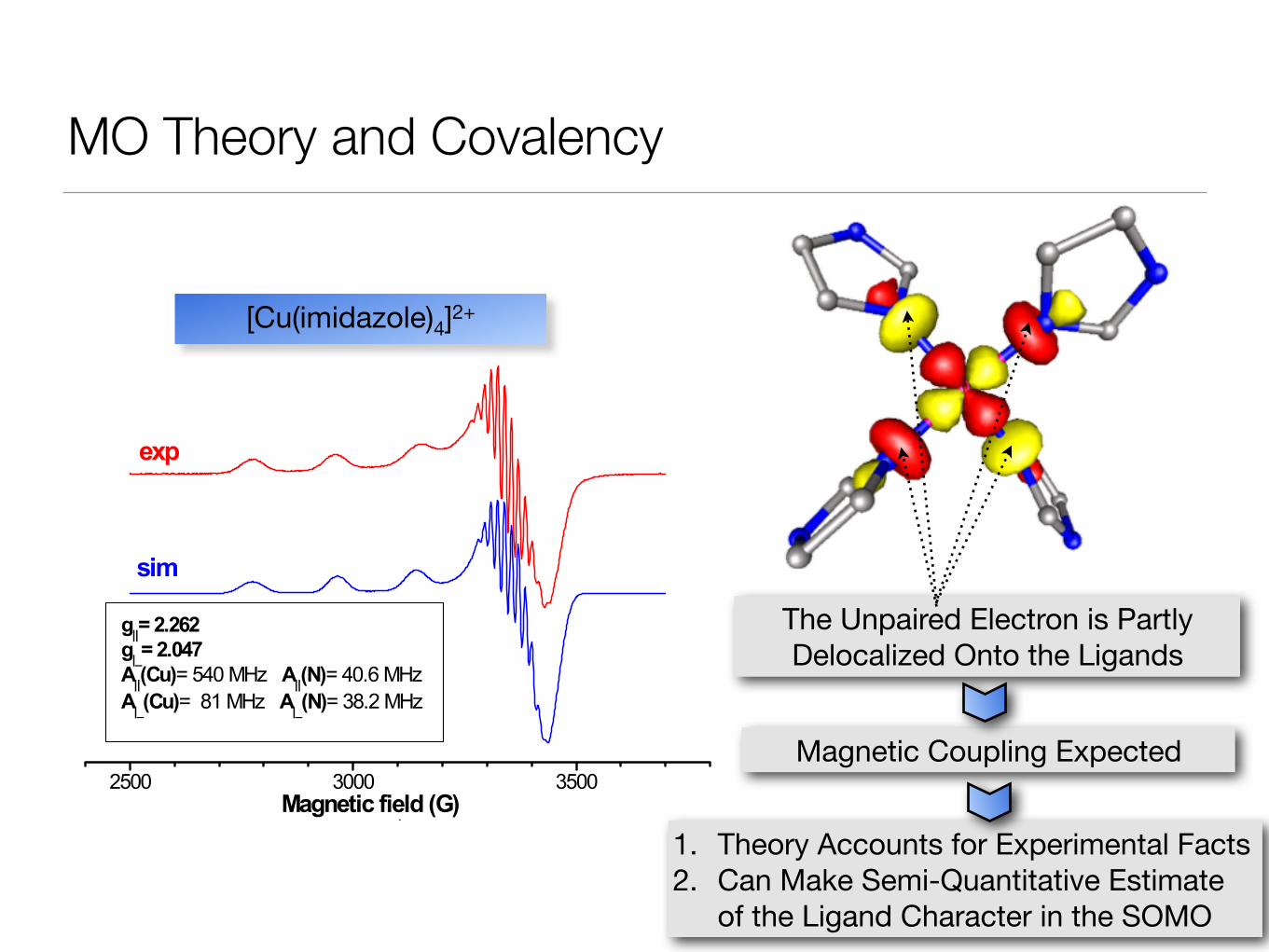
[Cu(imidazole)4]2+

The Unpaired Electron is Partly Delocalized Onto the Ligands

Magnetic Coupling Expected

1. Theory Accounts for Experimental Facts2. Can Make Semi-Quantitative Estimate

of the Ligand Character in the SOMO

MO Theory and Covalency

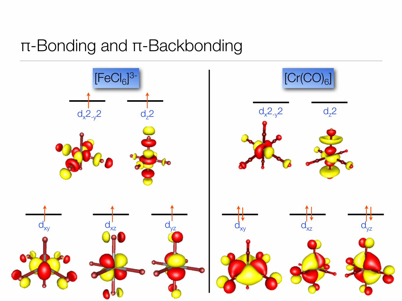
π-Bonding and π-Backbonding

[FeCl6]3- [Cr(CO)6]

dxy dxz dyzdxy dxz dyz

dz2 dz2dx2-y2 dx2-y2

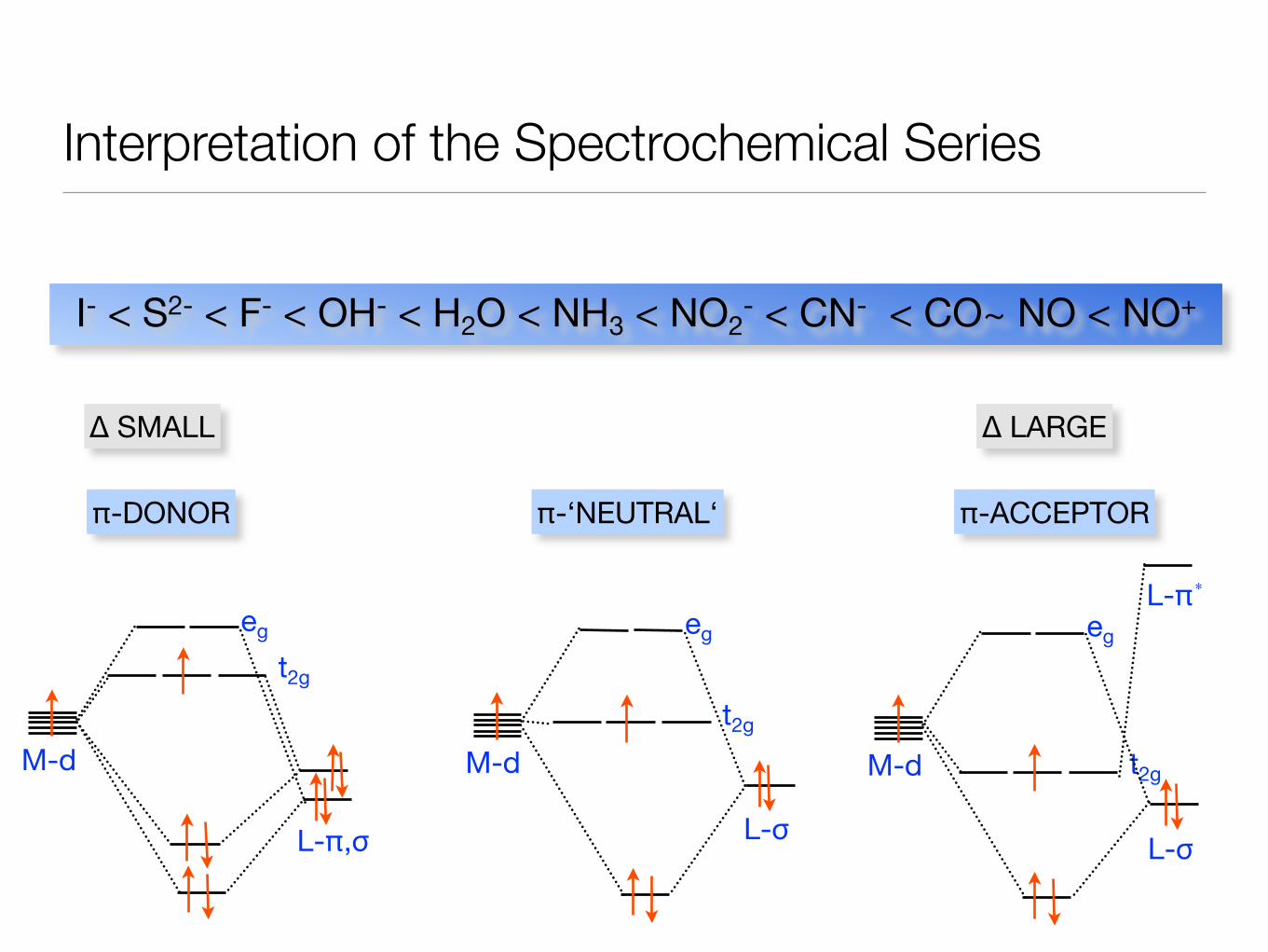
Interpretation of the Spectrochemical Series

Δ LARGEΔ SMALL

I- < S2- < F- < OH- < H2O < NH3 < NO2- < CN- < CO~ NO < NO+

π-DONOR π-ACCEPTORπ-‘NEUTRAL‘

L-π,σ

M-d

eg

t2g

L-σ

M-d

eg

t2g

L-σ

M-d

eg

t2g

L-π∗

Covalency, Oxidation States and MO Theory

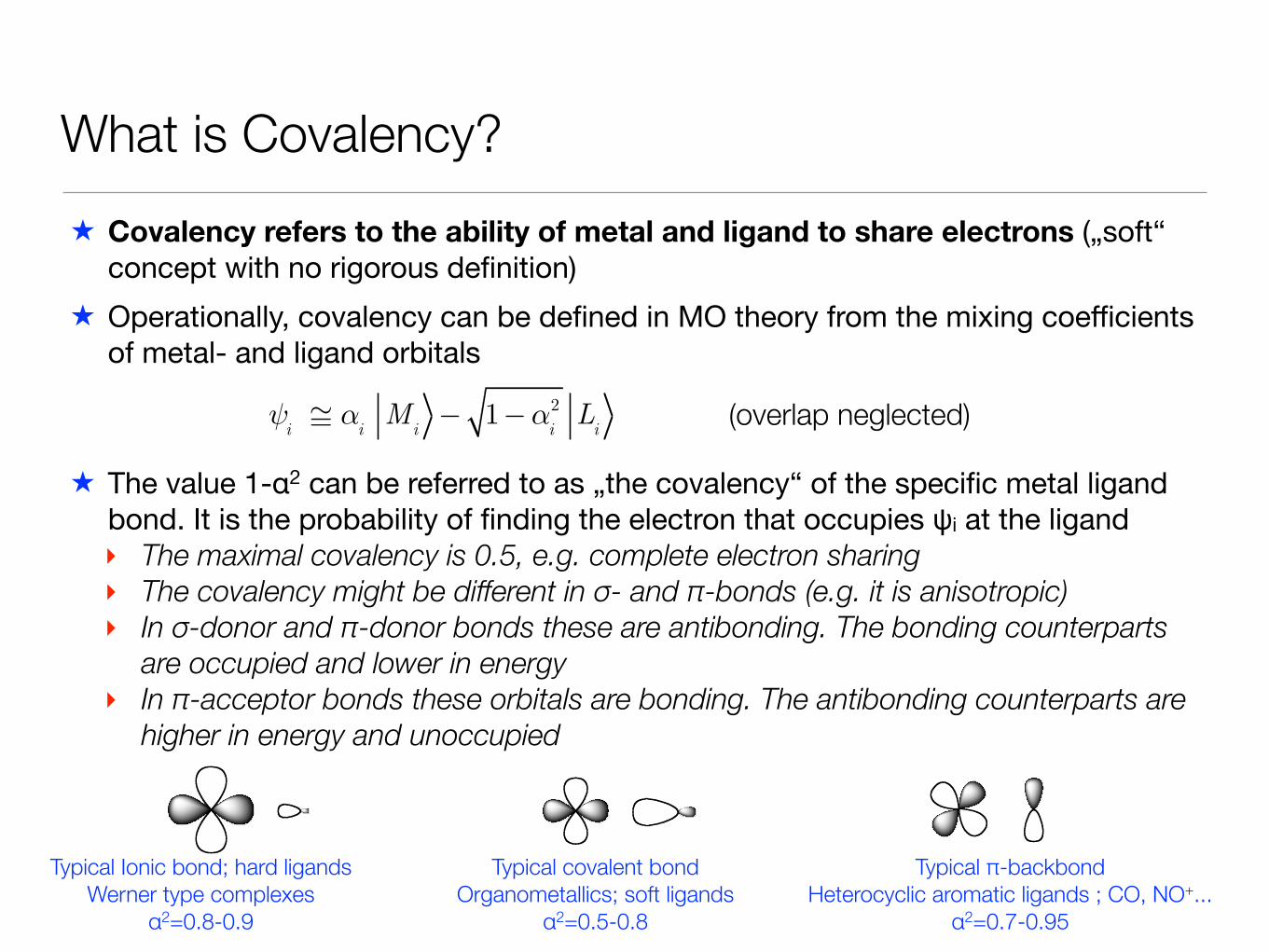
What is Covalency?★ Covalency refers to the ability of metal and ligand to share electrons („soft“

concept with no rigorous definition)★ Operationally, covalency can be defined in MO theory from the mixing coefficients

of metal- and ligand orbitals

ψ

i≅ α

iM

i− 1−α

i2 L

i (overlap neglected)

★ The value 1-α2 can be referred to as „the covalency“ of the specific metal ligand bond. It is the probability of finding the electron that occupies ψi at the ligand‣ The maximal covalency is 0.5, e.g. complete electron sharing ‣ The covalency might be different in σ- and π-bonds (e.g. it is anisotropic) ‣ In σ-donor and π-donor bonds these are antibonding. The bonding counterparts

are occupied and lower in energy ‣ In π-acceptor bonds these orbitals are bonding. The antibonding counterparts are

higher in energy and unoccupied

Typical Ionic bond; hard ligands Werner type complexes

α2=0.8-0.9

Typical covalent bond Organometallics; soft ligands

α2=0.5-0.8

Typical π-backbond Heterocyclic aromatic ligands ; CO, NO+...

α2=0.7-0.95

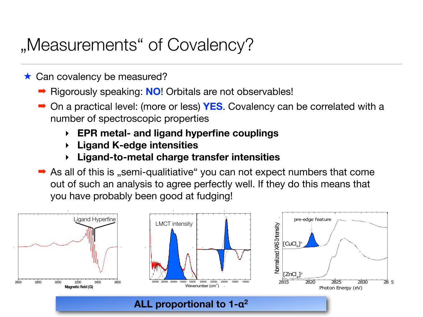
„Measurements“ of Covalency?★ Can covalency be measured?

➡ Rigorously speaking: NO! Orbitals are not observables!➡ On a practical level: (more or less) YES. Covalency can be correlated with a

number of spectroscopic properties ‣ EPR metal- and ligand hyperfine couplings ‣ Ligand K-edge intensities ‣ Ligand-to-metal charge transfer intensities

➡ As all of this is „semi-qualitiative“ you can not expect numbers that come out of such an analysis to agree perfectly well. If they do this means that you have probably been good at fudging!

Ligand HyperfineLMCT intensity

ALL proportional to 1-α2

Covalency and Molecular Properties

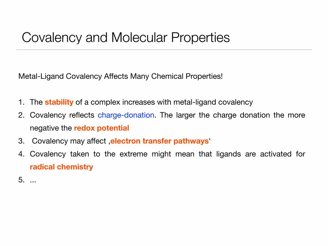
Metal-Ligand Covalency Affects Many Chemical Properties!!1. The stability of a complex increases with metal-ligand covalency2. Covalency reflects charge-donation. The larger the charge donation the more

negative the redox potential3. Covalency may affect ‚electron transfer pathways‘4. Covalency taken to the extreme might mean that ligands are activated for

radical chemistry5. ...

Covalency and Ligand-to-Metal Charge Transfer Spectra

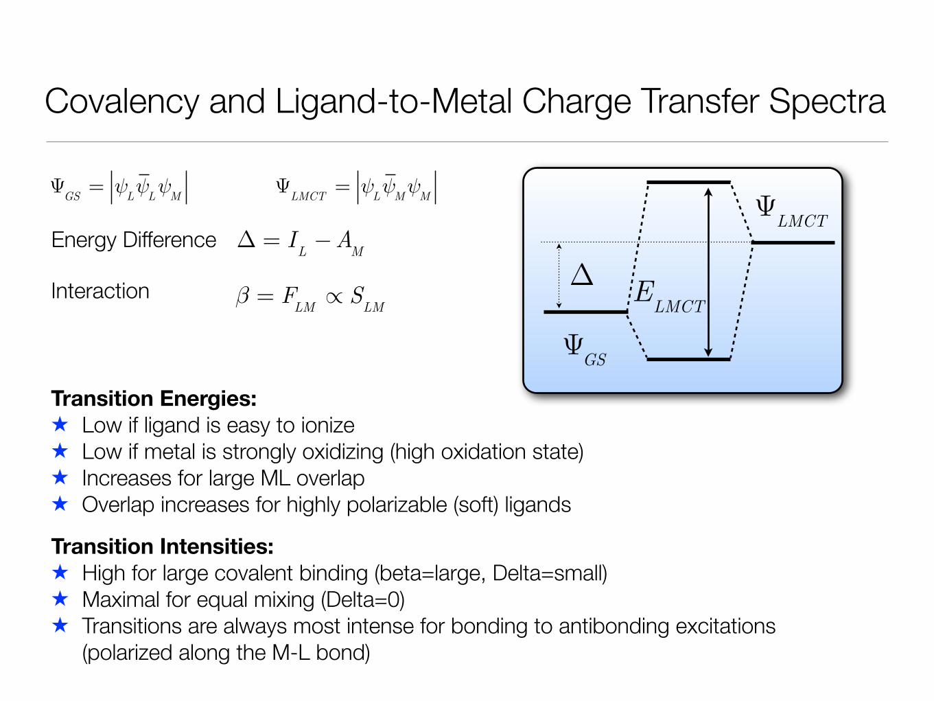
Ψ

GS= ψ

Lψ

Lψ

M Ψ

LMCT= ψ

Lψ

Mψ

M

Energy Difference Δ = IL−A

M

Interaction β = F

LM∝ S

LM

ΨGS

ΨLMCT

ELMCT Δ

Transition Energies: ★ Low if ligand is easy to ionize ★ Low if metal is strongly oxidizing (high oxidation state) ★ Increases for large ML overlap ★ Overlap increases for highly polarizable (soft) ligands

Transition Intensities: ★ High for large covalent binding (beta=large, Delta=small) ★ Maximal for equal mixing (Delta=0) ★ Transitions are always most intense for bonding to antibonding excitations

(polarized along the M-L bond)

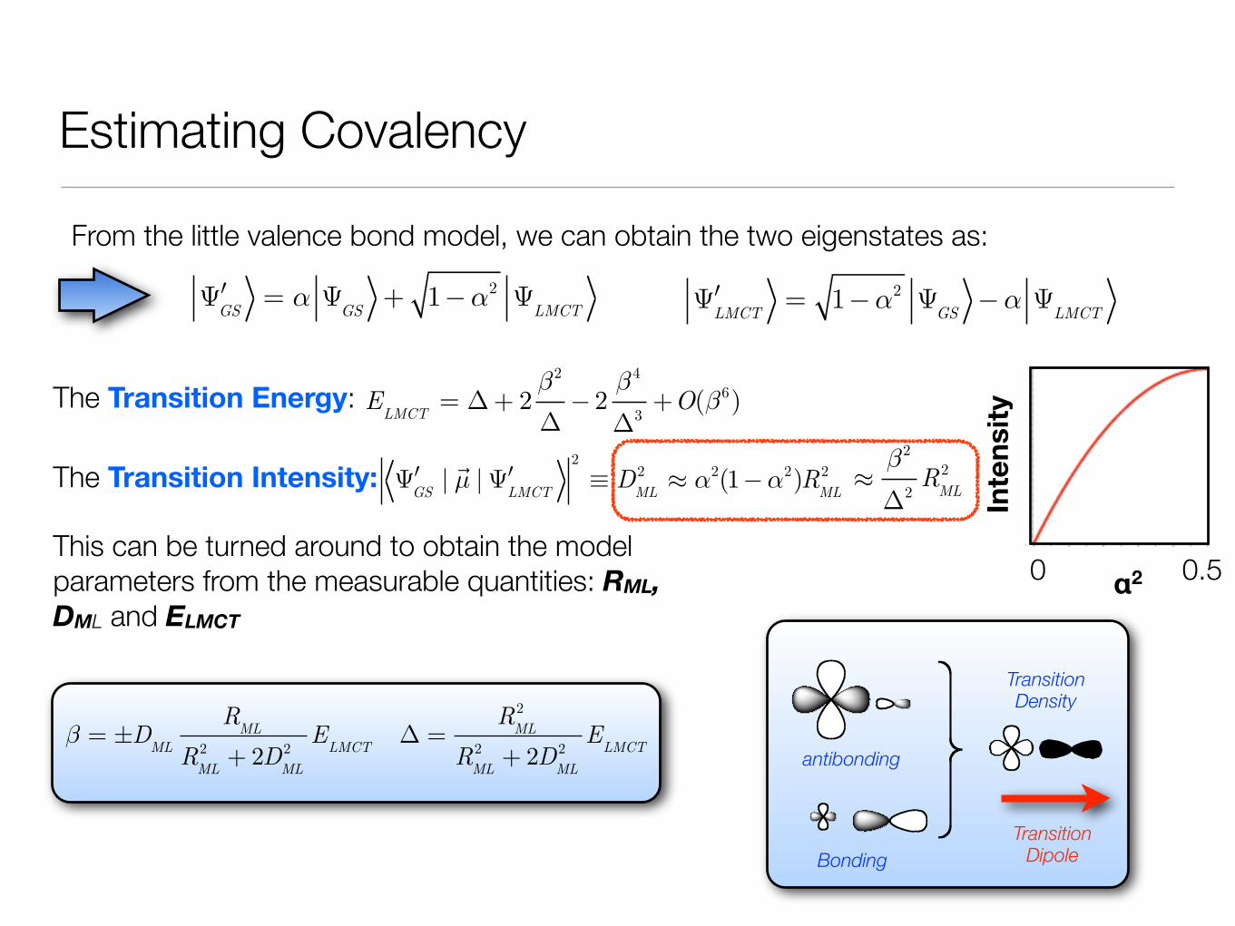
Estimating Covalency

E

LMCT= Δ+ 2

β2

Δ− 2β4

Δ3+O(β6)

′ΨGS

|!µ | ′Ψ

LMCT

2

≡ DML2 ≈ α2(1−α2)R

ML2

≈β2

Δ2R

ML2

β = ±DML

RML

RML2 + 2D

ML2

ELMCT

Δ =R

ML2

RML2 + 2D

ML2

ELMCT

′ΨGS

= α ΨGS

+ 1−α2 ΨLMCT

′ΨLMCT

= 1−α2 ΨGS−α Ψ

LMCT

From the little valence bond model, we can obtain the two eigenstates as:

The Transition Energy:

The Transition Intensity:

This can be turned around to obtain the model parameters from the measurable quantities: RML, DML and ELMCT

Bonding

antibonding

Transition Density

Transition Dipole

Inte

nsity

α20 0.5

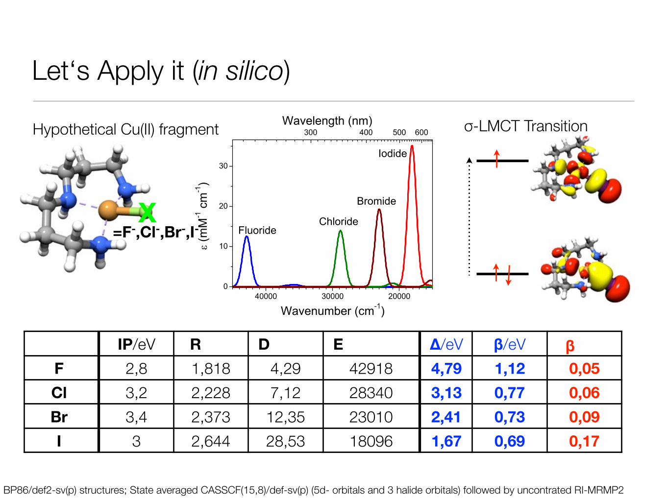
Let‘s Apply it (in silico)

IP/eV R D E Δ/eV β/eV βF 2,8 1,818 4,29 42918 4,79 1,12 0,05Cl 3,2 2,228 7,12 28340 3,13 0,77 0,06Br 3,4 2,373 12,35 23010 2,41 0,73 0,09I 3 2,644 28,53 18096 1,67 0,69 0,17

X=F-,Cl-,Br-,I-

Hypothetical Cu(II) fragment

BP86/def2-sv(p) structures; State averaged CASSCF(15,8)/def-sv(p) (5d- orbitals and 3 halide orbitals) followed by uncontrated RI-MRMP2

σ-LMCT Transition

Exchange CouplingThe Spin State Problem:

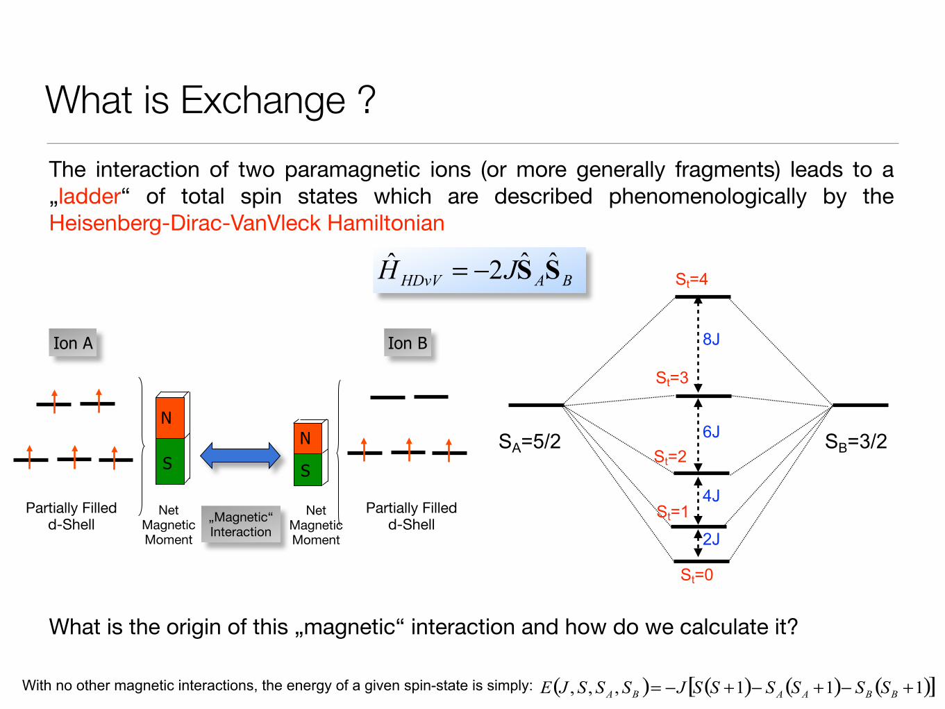
What is Exchange ?The interaction of two paramagnetic ions (or more generally fragments) leads to a „ladder“ of total spin states which are described phenomenologically by the Heisenberg-Dirac-VanVleck Hamiltonian

Ion A Ion B

Partially Filledd-Shell

Partially Filledd-Shell

Net MagneticMoment

Net MagneticMoment

N

SN

S

„Magnetic“Interaction

SA=5/2 SB=3/2

2J

4J

St=0

St=4

St=1

6J

8J

St=2

St=3

With no other magnetic interactions, the energy of a given spin-state is simply:

What is the origin of this „magnetic“ interaction and how do we calculate it?

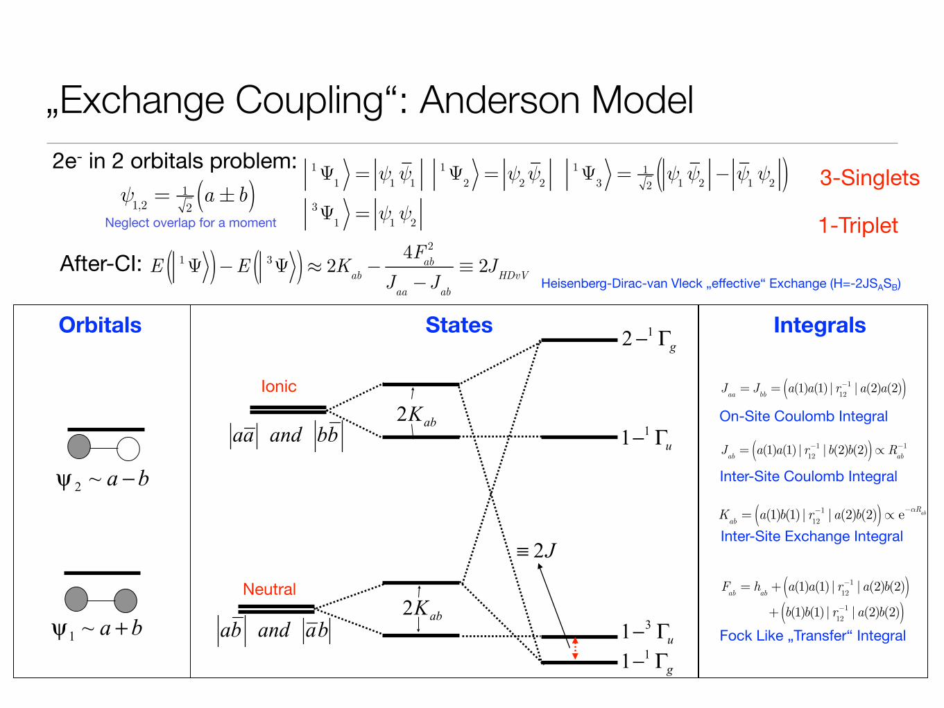
„Exchange Coupling“: Anderson Model2e- in 2 orbitals problem:

3-Singlets

1-TripletAfter-CI:

Orbitals States Integrals

On-Site Coulomb Integral

Inter-Site Coulomb Integral

Inter-Site Exchange Integral

Fock Like „Transfer“ Integral

Neutral

Ionic

Neglect overlap for a moment

Heisenberg-Dirac-van Vleck „effective“ Exchange (H=-2JSASB)

ψ1,2= 1

2a ±b( )

1Ψ1= ψ

1ψ1

1Ψ2= ψ

2ψ2

1Ψ3= 1

2ψ1ψ2− ψ

1ψ2( )

3Ψ1= ψ

1ψ2

E1Ψ( )−E 3Ψ( )≈ 2Kab − 4F

ab

2

Jaa−J

ab

≡ 2JHDvV

Jaa= J

bb= a(1)a(1) | r

12−1 |a(2)a(2)( )

Jab= a(1)a(1) | r

12−1 |b(2)b(2)( )∝ Rab−1

Kab= a(1)b(1) | r

12−1 |a(2)b(2)( )∝ e−αRab

Fab= h

ab+ a(1)a(1) | r

12−1 |a(2)b(2)( )

+ b(1)b(1) | r12−1 |a(2)b(2)( )