Embed Size (px)
Citation preview

Lifshitz Tails in Constant Magnetic Fields
Frederic Klopp, Georgi Raikov
Abstract: We consider the 2D Landau Hamiltonian H perturbed by a random alloy-type
potential, and investigate the Lifshitz tails, i.e. the asymptotic behavior of the corresponding
integrated density of states (IDS) near the edges in the spectrum of H. If a given edge coin-
cides with a Landau level, we obtain different asymptotic formulae for power-like, exponential
sub-Gaussian, and super-Gaussian decay of the one-site potential. If the edge is away from the
Landau levels, we impose a rational-flux assumption on the magnetic field, consider compactly
supported one-site potentials, and formulate a theorem which is analogous to a result obtained
by the first author and T. Wolff in [25] in the case of a vanishing magnetic field.
2000 AMS Mathematics Subject Classification: 82B44, 47B80, 47N55, 81Q10
Key words: Lifshitz tails, Landau Hamiltonian, continuous Anderson model
1 Introduction
LetH0 = H0(b) := (−i∇− A)2 − b (1.1)
be the unperturbed Landau Hamiltonian, essentially self-adjoint on C∞0 (R2). Here A =(− bx2
2, bx1
2) is the magnetic potential, and b ≥ 0 is the constant scalar magnetic field. It
is well-known that if b > 0, then the spectrum σ(H0) of the operator H0(b) consists ofthe so-called Landau levels 2bq, q ∈ Z+, and each Landau level is an eigenvalue of infinitemultiplicity. If b = 0, then H0 = −∆, and σ(H0) = [0,∞) is absolutely continuous.Next, we introduce a random Z2-ergodic alloy-type electric potential
V (x) = Vω(x) :=∑
γ∈Z2
ωγu(x− γ), x ∈ R2.
Our general assumptions concerning the potential Vω are the following ones:
• H1: The single-site potential u satisfies the estimates
0 ≤ u(x) ≤ C0(1 + |x|)−κ, x ∈ R2, (1.2)
with some κ > 2 and C0 > 0. Moreover, there exists an open non-empty setΛ ⊂ R2 and a constant C1 > 0 such that u(x) ≥ C1 for x ∈ Λ.
1

• H2: The coupling constants {ωγ}γ∈Z2 are non-trivial, almost surely bounded i. i.d. random variables.
Evidently, these two assumptions entail
M := ess-supω
supx∈R2
|Vω(x)| <∞. (1.3)
On the domain of H0 define the operator H = Hω := H0(b)+Vω. The integrated densityof states (IDS) for the operator H is defined as a non-decreasing left-continuous functionNb : R→ [0,∞) which almost surely satisfies
∫
Rϕ(E)dNb(E) = lim
R→∞R−2Tr (1ΛRϕ(H)1ΛR) , ∀ϕ ∈ C∞0 (R). (1.4)
Here and in the sequel 1O denotes the the characteristic function of the set O, and
ΛR :=(−R
2, R
2
)2. By the Pastur-Shubin formula (see e.g. [36, Section 2] or [11, Corollary
3.3]) we have
∫
Rϕ(E)dNb(E) = E (Tr (1Λ1ϕ(H)1Λ1)) , ∀ϕ ∈ C∞0 (R), (1.5)
where E denotes the mathematical expectation. Moreover, there exists a set Σ ⊂ Rsuch that σ(Hω) = Σ almost surely, and supp dNb = Σ. The aim of the present articleis to study the asymptotic behavior of Nb near the edges of Σ. It is well known that,for many random models, this behavior is characterized by a very fast decay which goesunder the name of “Lifshitz tails”. It was studied extensively in the absence of magneticfield (see e.g. [31], [15]), and also in the presence of magnetic field for other types ofdisorder (see [2], [6], [12], [7], [13]).
2 Main results
In order to fix the picture of the almost sure spectrum σ(Hω), we assume b > 0, andmake the following two additional hypotheses:
• H3: The support of the random variables ωγ , γ ∈ Z2, consists of the interval[ω−, ω+] with ω− < ω+ and ω−ω+ ≤ 0.
• H4: We have M+ −M− < 2b where ±M± := ess-supω supx∈R2 (±Vω(x)).
Assumptions H1 – H4 imply M−M+ ≤ 0. Moreover, the union ∪∞q=0[2bq+M−, 2bq+M+]which contains Σ, is disjoint. Introduce the bounded Z2-periodic potential
W (x) :=∑
γ∈Z2
u(x− γ), x ∈ R2,
2

and on the domain of H0 define the operators H± := H0 + ω±W . It is easy to see that
σ(H−) ⊆ ∪∞q=0[2bq +M−, 2bq], σ(H+) ⊆ ∪∞q=0[2bq, 2bq +M+],
and
σ(H−) ∩ [2bq +M−, 2bq] 6= ∅, σ(H+) ∩ [2bq, 2bq +M+] 6= ∅, ∀q ∈ Z+.
Set
E−q := inf{σ(H−) ∩ [2bq +M−, 2bq]
}, E+
q := sup{σ(H+) ∩ [2bq, 2bq +M+]
}.
Following the argument in [16] (see also [31, Theorem 5.35]), we easily find that
Σ = ∪∞q=0[E−q , E+q ],
i.e. Σ is represented as a disjoint union of compact intervals, and each interval [E−q , E+q ]
contains exactly one Landau level 2bq, q ∈ Z+.In the following theorems we describe the behavior of the integrated density of statesNb near E−q , q ∈ Z+; its behavior near E+
q could be analyzed in a completely analogousmanner.Our first theorem concerns the case where E−q = 2bq, q ∈ Z+. This is the case if andonly if ω− = 0; in this case, the random variables ωγ, γ ∈ Z2, are non-negative.
Theorem 2.1. Let b > 0 and assumptions H1 – H4 hold. Suppose that ω− = 0, andthat
P(ω0 ≤ E) ∼ CEκ, E ↓ 0, (2.1)
for some C > 0 and κ > 0. Fix the Landau level 2bq = E−q , q ∈ Z+.i) Assume that C−(1 + |x|)−κ ≤ u(x) ≤ C+(1 + |x|)−κ, x ∈ R2, for some κ > 2, andC+ ≥ C− > 0. Then we have
limE↓0
ln | ln (Nb(2bq + E)−Nb(2bq))|lnE
= − 2
κ − 2. (2.2)
ii) Assume e−C+|x|β
C+≤ u(x) ≤ e−C−|x|
β
C−, x ∈ R2, β ∈ (0, 2], C+ ≥ C− > 0. Then we have
limE↓0
ln | ln (Nb(2bq + E)−Nb(2bq))|ln | lnE| = 1 +
2
β. (2.3)
iii) Assume1{x∈R2 ; |x−x0|<ε}
C+≤ u(x) ≤ e−C−|x|
2
C−for some C+ ≥ C− > 0, x0 ∈ R2, and
ε > 0. Then there exists δ > 0 such that
1 + δ ≤ lim infE↓0
ln | ln (Nb(2bq + E)−Nb(2bq)|ln | lnE| ≤
lim supE↓0
ln | ln (Nb(2bq + E)−Nb(2bq)|ln | lnE| ≤ 2. (2.4)
3

The proof of Theorem 2.1 is contained in Sections 3 – 5. In Section 3 we constructa periodic approximation of the IDS Nb which plays a crucial role in this proof. Theupper bounds of the IDS needed for the proof of Theorem 2.1 are obtained in Section4, and the corresponding lower bounds are deduced in Section 5.Remarks: i) In the first and second part of Theorem 2.1 we consider one-site potentials urespectively of power-like or exponential sub-Gaussian decay at infinity, and obtain thevalues of the so called Lifshitz exponents. Note however that in the case of power-likedecay of u the double logarithm of Nb(2bq+E)−N (2bq) is asymptotically proportionalto lnE (see (2.2)), while in the case of exponentially decaying u this double logarithm isasymptotically proportional to ln | lnE| (see (2.3)); in both cases the Lifshitz exponentis defined as the corresponding proportionality factor. In the third part of the theoremwhich deals with one-site potentials u of super-Gaussian decay, we obtain only upperand lower bounds of the Lifshitz exponent. It is natural to conjecture that the valueof this exponent is 2, i.e. that the upper bound in (2.4) reveals the correct asymptoticbehavior.ii) In the case of a vanishing magnetic field, the Lifshitz asymptotics for random Schro-dinger operator with repulsive random alloy-type potentials has been known since longago (see [17]). To the authors’ best knowledge the Lifshitz asymptotics for the LandauHamiltonian with non-zero magnetic field, perturbed by a positive random alloy-typepotential, is considered for the first time in the present article. However, it is appropriateto mention here the related results concerning the Landau Hamiltonian with repulsiverandom Poisson potential. In [2] the Lifshitz asymptotics in the case of a power-likedecay of the one-site potential u, was investigated. The case of a compact support of uwas considered in [6]. The results for the case of a compact support of u were essentiallyused in [12] and [7] (see also [13]), in order to study the problem in the case of anexponential decay of u.Our second theorem concerns the case where E−q < 2bq, q ∈ Z+. This is the case ifand only if ω− < 0. In order to handle this case, we need some facts from the magneticFloquet-Bloch theory. Let Γ := g1Z⊕ g2Z with gj > 0, j = 1, 2. Introduce the tori
TΓ := R2/Γ, T∗Γ := R2/Γ∗, (2.5)
where Γ∗ := 2πg−11 Z ⊕ 2πg−1
2 Z is the lattice dual to Γ. Denote by OΓ and O∗Γ thefundamental domains of TΓ and T∗Γ respectively. Let W : R2 → R be a Γ-periodicbounded real-valued function. On the domain of H0 define the operator HW := H0 +W .Assume that the scalar magnetic field b ≥ 0 satisfies the integer-flux condition withrespect to the lattice Γ, i.e. that bg1g2 ∈ 2πZ+. Fix θ ∈ T∗Γ. Denote by h0(θ) theself-adjoint operator generated in L2(OΓ) by the closure of the non-negative quadraticform ∫
OΓ
|(i∇+ A− θ)f |2dx
4

defined originally on the set
{f = g∣∣OΓ
| g ∈ C∞(R2), (τγg)(x) = g(x), x ∈ R2, γ ∈ Γ
}
where τy, y ∈ R2, is the magnetic translation given by
(τyg)(x) := eiby1y2
2 eibx∧y
2 g(x+ y), x ∈ R2, (2.6)
with x∧y := x1y2−x2y1. Note that the integer-flux condition implies that the operatorsτγ, γ ∈ Γ, commute with each other, as well as with operators i ∂
∂xj+ Aj, j = 1, 2 (see
(1.1)), and hence with H0 and HW . In the case b = 0, the domain of the operator h0 isisomorphic to the Sobolev space H2(TΓ), but if b > 0, this is not the case even underthe integer-flux assumption since h0 acts on U(1)-sections rather than on functions overTΓ (see e.g [30, Subsection 2.2]). On the domain of h0 define the operator
hW(θ) := h0(θ) +W , θ ∈ T∗Γ. (2.7)
Set
H0 :=
∫
O∗Γ⊕ h0(θ)dθ, HW :=
∫
O∗Γ⊕ hW(θ)dθ. (2.8)
It is well-known (see e.g [10], [35], or [30, Subsection 2.4]) that the operators H0 andHW are unitarily equivalent to the operators H0 and HW respectively. More precisely,we have H0 = U∗H0U and HW = U∗HWU where U : L2(R2) → L2(OΓ × O∗Γ) is theunitary Gelfand-type operator defined by
(Uf)(x; θ) :=1√
volT∗Γ
∑
γ∈Γ
e−iθ(x+γ)(τγf)(x), x ∈ OΓ, θ ∈ T∗Γ. (2.9)
Evidently for each θ ∈ T∗Γ the spectrum of the operator hW(θ) is purely discrete. Denoteby {Ej(θ)}∞j=1 the non-decreasing sequence of its eigenvalues. Let E ∈ R. Set
J(E) := {j ∈ N ; there exists θ ∈ T∗Γ such that Ej(θ) = E} .
Evidently, for each E ∈ R the set J(E) is finite. If E ∈ R is an end of an open gapin σ(H0 +W), then we will call it an edge in σ(H0 +W). We will call the edge E inσ(H0 +W) simple if #J(E) = 1. Moreover, we will call the edge E non-degenerate iffor each j ∈ J(E) the number of points θ ∈ T∗Γ such that Ej(θ) = E is finite, and ateach of these points the extremum of Ej is non-degenerate.Assume at first that b = 0. Then H0 = −∆, and we will consider the general d-dimensional situation; the simple and non-degenerate edges in σ(−∆ +W) are definedexactly as in the two-dimensional case. IfW : Rd → R is a real-valued bounded periodicfunction, it is well-known that:
5

• The spectrum of −∆+W is absolutely continuous (see e.g. [33, Theorems XIII.90,XIII.100]). In particular, no Floquet eigenvalue Ej : T∗Γ → R, j ∈ N, is constant.
• If d = 1, all the edges in σ(−∆ +W) are simple and non-degenerate (see e.g. [33,Theorem XIII.89]).
• For d ≥ 1 the bottom of the spectrum of −∆ +W is a simple and non-degenerateedge (see [19]).
• For d ≥ 1, the edges of σ(−∆ +W) generically are simple (see [24]).
Despite the widely spread belief that generically the higher edges in σ(−∆ +W) shouldalso be non-degenerate in the multi-dimensional case d > 1, there are no rigorous resultsin support of this conjecture.Let us go back to the investigation of the Lifshitz tails for the operator −∆ + Vω. Itfollows from the general results of [16] that E− (respectively, E+) is an upper (respec-tively, lower) end of an open gap in σ(−∆+Vω) if and only if it is an upper (respectively,lower) end of an open gap in the spectrum of −∆ + ω−W (respectively, −∆ + ω+W ).For definiteness, let us consider the case of an upper end E−. The asymptotic behaviorof the IDS N0(E) as E ↓ E− has been investigated in [28] - [29] in the case d = 1, andin [19] in the case d ≥ 1 and E− = inf σ(−∆ + ω−W ). Note that the proofs of theresults of [28], [29], and [19], essentially rely on the non-degeneracy of E−. Later, theLifshitz tails for the operator −∆ +Vω near the edge E− were investigated in [15] underthe assumptions that d ≥ 1, E− > inf σ(−∆ + ω−W ), and that E− is non-degenerateedge in the spectrum of −∆ + ω−W ; due to the last assumption these results are con-ditional. However, it turned out possible to lift the non-degeneracy assumption in thetwo-dimensional case considered in [25]. First, it was shown in [25, Theorem 0.1] thatfor any single-site potential u satisfying assumption H1, we have
lim supE↓0
ln | ln (N0(E− + E)−N0(E−q ))|lnE
< 0
without any additional assumption on E−. If, moreover, the support of u is compact,and the probability P(ω0−ω− ≤ E) admits a power-like decay as E ↓ 0, it follows from[25, Theorem 0.2] that there exists α > 0 such that
limE↓0
ln | ln (N0(E− + E)−N0(E−q ))|lnE
= −α (2.10)
under the unique generic hypothesis that E− is a simple edge. Note that the absolutecontinuity of σ(−∆ + ω−W ) plays a crucial role in the proofs of the results of [25].Assume now that the scalar magnetic field b > 0 satisfies the rational flux conditionb ∈ 2πQ. More precisely, we assume that b/2π is equal to the irreducible fraction p/r,p ∈ N, r ∈ N. Then b satisfies the integer-flux assumption with respect, say, to thelattice Γ = rZ ⊕ Z, and the operator H− is unitarily equivalent to Hω−W . As in the
6

non-magnetic case, in order to investigate the Lifshitz asymptotics as E ↓ E−q of Nb(E),we need some information about the character of E−q as an edge in the spectrum of H−.For example, if we assume that E−q is a simple edge, and the corresponding Floquetband does not shrink into a point, we can repeat almost word by word the argument ofthe proof of [25, Theorem 0.2], and obtain the following
Theorem 2.2. Let b > 0, b ∈ 2πQ, and assumptions H1 – H4 hold. Assume that thesupport of u is compact, ω− < 0, and P(ω0 − ω− ≤ E) ∼ CEκ, E ↓ 0, for some C > 0and κ > 0. Fix q ∈ Z+. Suppose E−q is a simple edge in the spectrum of the operatorH−, and that the function Ej, j ∈ J(E−q ), is not identically constant. Then there existsα > 0 such that
limE↓0
ln | ln (Nb(E−q + E)−Nb(E−q ))|lnE
= −α. (2.11)
Remarks: i) It is believed that under the rational-flux assumption the Floquet eigen-values Ej, j ∈ N, for the operator H− generically are not constant. Note that thisproperty may hold only generically due to the obvious counterexample where u = 1Λ1 ,H− = H0 + ω−, and for all j ∈ N the Floquet eigenvalue Ej is identically equal to2b(j− 1) +ω−. Also, in contrast to the non-magnetic case, we do not know whether theedges in the spectrum of H− generically are simple.ii) The definition of the constant α in (2.11) is completely analogous to the one in (2.10)which concerns the non-magnetic case. This definition involving the concepts of Newtonpolygon, Newton diagram, and Newton decay exponent, is not trivial, and can be foundin the original work [25], or in [22, Subsection 4.2.8].
3 Periodic approximation
Pick a > 0 such that ba2
2π∈ N. Set L := (2n + 1)/2, n ∈ N, and define the random
2LZ2-periodic potential
V per(x) = V pern,ω (x) :=
∑
γ∈2LZ2
(Vω1Λ2L) (x+ γ), x ∈ R2.
On the domain of H0 define the operator Hper = Hpern,ω := H0 + V per
n,ω . For brevity setT2L := T2LZ2 , T∗2L := T∗2LZ2 (see (2.5)). Note that the square Λ2L is the fundamentaldomain of the torus T2L, while Λ∗2L := ΛπL−1 is the fundamental domain of T∗2L. As in(2.7), on the domain of h0 define the operator
h(θ) = hper(θ) := h0(θ) + V per, θ ∈ T∗2L,
and by analogy with (2.8) set
Hper :=
∫
Λ∗2L
⊕ hper(θ)dθ.
7
As above, the operators H0 and Hper are unitarily equivalent to the operators H0 andHper respectively. Set
N per(E) = N pern,ω (E) := (2π)−2
∫
Λ∗2L
N(E;hper(θ))dθ, E ∈ R. (3.1)
Here and in the sequel, if T is a self-adjoint operator with purely discrete spectrum,then N(E;T ) denotes the number of the eigenvalues of T less than E ∈ R, and countedwith the multiplicities. The function N per plays the role of IDS for the operator Hper
since, similarly to (1.4) and (1.5), we have∫
Rϕ(E)dN per(E) = lim
R→∞R−2Tr (1ΛRϕ(Hper)1ΛR)
almost surely, and
E(∫
Rϕ(E)dN per(E)
)= E (Tr (1Λ1ϕ(Hper)1Λ1)) , (3.2)
for any ϕ ∈ C∞0 (R) (see e.g. the proof of [21, Theorem 5.1] where however the case ofa vanishing magnetic field is considered).
Theorem 3.1. Assume that hypotheses H1 and H2 hold. Let q ∈ Z+, η > 0. Thenthere exist ν > 0 and E0 > 0 such that for E ∈ (0, E0] and n ≥ E−ν we have
E (N per(2bq + E/2)−N per(2bq − E/2))− e−E−η ≤ Nb(2bq + E)−Nb(2bq − E) ≤
E (N per(2bq + 2E)−N per(2bq − 2E)) + e−E−η. (3.3)
The main technical steps of the proof of Theorem 3.1 which is the central result of thissection, are contained in Lemmas 3.1 and 3.2 below.
Lemma 3.1. Let Q = Q ∈ L∞(R2), X := H0 + Q, D(X) = D(H0). Then there existsε = ε(b) > 0 such that for each α, β ∈ Z2, and z ∈ C \ σ(X) we have
‖χα(X − z)−1χβ‖HS ≤ 2b+ 1
π1/2
(1 +
1
η(z)
)e−εη(z)|α−β| (3.4)
where χα := 1Λ1+α, α ∈ Z2, η(z) = η(z; b,Q) := dist(z,σ(X))|z|+|Q|∞+1
, ‖ · ‖HS denotes the Hilbert-
Schmidt norm, and |Q|∞ := ‖Q‖L∞(R2).
Proof. We will apply the ideas of the proof of [20, Proposition 4.1]. For ξ ∈ R2 set
Xξ := eξ·xXe−ξ·x = (i∇+ A− iξ)2 +Q = X − 2iξ · (i∇+ A) + |ξ|2.
Evidently,
Xξ − z = (X − z)(1 + (X − z)−1
(|ξ|2 − 2iξ · (i∇+ A)
)). (3.5)
8

Let us estimate the norm of the operator (X − z)−1 (|ξ|2 − 2iξ · (i∇+ A)) appearing atthe right-hand side of (3.5). We have
‖(X − z)−1|ξ|2‖ ≤ |ξ|2dist(z, σ(X))−1,
‖(X − z)−12iξ · (i∇+ A)‖ ≤2‖(H0 + 1)−1(i∇+ A) · ξ − (X − z)−1(Q− z − 1)(H0 + 1)−1(i∇+ A) · ξ‖ ≤
2C
(1 +
1
η(z)
)|ξ|
with
C = C(b) := ‖(H0 + 1)−1(i∇+ A)‖ = supq∈Z+
((2q + 1)b)1/2
2bq + 1.
Choose ε ∈(
0, 18(C+1)
)and ξ ∈ R2 such that |ξ| = εη(z). Then, by the above estimates,
we have
‖(X − z)−1(|ξ|2 − 2iξ · (i∇+ A)
)‖ ≤ ε2η(z)2dist(z, σ(X))−1 + 2Cε
(1 +
1
η(z)
)η(z) ≤
ε2η(z) + 2Cε(1 + η(z)) < ε2 + 4Cε < 3/4 (3.6)
since the resolvent identity implies η(z) < 1. Therefore, the operator Xξ−z is invertible,and
χα(X − z)−1χβ =(e−ξ·xχα
)χα(Xξ − z)−1χβ
(eξ·xχβ
). (3.7)
Moreover, (3.5) and (3.6) imply
‖χα(Xξ − z)−1χβ‖HS ≤ 4‖(X − z)−1χβ‖HS ≤4‖(H0 + 1)−1χβ − (X − z)−1(Q− z − 1)(H0 + 1)−1χβ‖HS ≤
4‖(H0+1)−1χβ‖HS(1+‖(X−z)−1(Q−z−1)‖) ≤ 4‖(H0+1)−1χβ‖HS
(1 +
1
η(z)
). (3.8)
Finally, applying the diamagnetic inequality for Hilbert-Schmidt operators (see e.g. [1]),we get
‖(H0 + 1)−1χβ‖HS ≤ ‖(H0 + 1)−1(H0 + b+ 1)‖‖(H0 + b+ 1)−1χβ‖HS ≤‖(H0 + 1)−1(H0 + b+ 1)‖‖(−∆ + 1)−1χβ‖HS =
supq∈Z+
2bq + b+ 1
2bq + 1‖(−∆ + 1)−1χβ‖HS =
b+ 1
2π1/2. (3.9)
The combination of (3.7), (3.8), and (3.9) yields
‖χα(X − z)−1χβ‖HS ≤2(b+ 1)
π1/2e−ξ(α−β)
(1 +
1
η(z)
).
Choosing ξ = εη(z) α−β|α−β| , we get (3.4).
9

Lemma 3.2. Assume that hypotheses H1 and H2 hold. Then there exists a constantC > 1 such that for any ϕ ∈ C∞0 (R), and any n ∈ N, l ∈ N, we have
∣∣∣∣E(∫
Rϕ(E)dNb(E)−
∫
Rϕ(E)dN per(E)
)∣∣∣∣ ≤
cn−leCl log l supx∈R, 0≤j≤l+5
∣∣∣∣(|x|+ C)l+5djϕ
dxj(x)
∣∣∣∣ . (3.10)
Proof. We will follow the general lines of the proof of [23, Lemma 2.1]. Due to the factthat we consider only the two-dimensional case, and an alloy-type potential which isalmost surely bounded, the argument here is somewhat simpler than the one in [23]. By(1.5) and (3.2) we have
E(∫
Rϕ(E)dNb(E)−
∫
Rϕ(E)dN per(E)
)= E (Tr (1Λ1(ϕ(H)− ϕ(Hper))1Λ1)) .
Next, we introduce a representation of the operator ϕ(H) − ϕ(Hper) by the Helffer-Sjostrand formula (see e.g. [4, Chapter 8]). Let ϕ be an almost analytic extension ofthe function ϕ ∈ C∞0 (R) appearing in (3.10). We recall that ϕ possesses the followingproperties:
1. If Im z = 0, then ϕ(z) = ϕ(z).
2. supp ϕ ⊂ {x+ iy ∈ C; |y| < 1}.
3. ϕ ∈ S ({x+ iy ∈ C; |y| < 1}).
4. The family of functions x 7→ ∂ϕ∂z
(x+ iy)|y|−m, |y| ∈ (0, 1), is bounded in S(R) forany m ∈ Z+.
Such extensions exist for ϕ ∈ S(R) (see [27], [4, Chapter 8]), and there exists a constantC > 1 such that for any m ≥ 0, α ≥ 0, β ≥ 0, we have
sup0≤|y|≤1
supx∈R
∣∣∣∣xα∂β
∂xβ
(|y|−m∂ϕ
∂z(x+ iy)
)∣∣∣∣ ≤
Cm logm+α logα+β+1 supβ′≤m+β+2, α′≤α
supx∈R
∣∣∣∣xα′ dβ
′ϕ(x)
dxβ′
∣∣∣∣ . (3.11)
Then the Helffer-Sjostrand formula yields
E (Tr (1Λ1(ϕ(H)− ϕ(Hper))1Λ1)) =
1
πE(
Tr
(∫
C
∂ϕ
∂z(z)(1Λ1
((H − z)−1 − (Hper − z)−1
)1Λ1
)dxdy
))=
10

1
πE(
Tr
(∫
C
∂ϕ
∂z(z)(1Λ1(H − z)−1(V per − V )(Hper − z)−11Λ1
)dxdy
)). (3.12)
Next, we will show that 1Λ1(H−z)−1(V per−V )(Hper−z)−11Λ1 is a trace-class operatorfor z ∈ C \ R, and almost surely
‖1Λ1(H − z)−1(V per − V )(Hper − z)−11Λ1‖Tr ≤M(b+ 1)2
2π
(1 +
M + |z|+ 1
|Im z|
)2
(3.13)
where ‖.‖Tr denotes the trace-class norm. Evidently,
‖1Λ1(H − z)−1(V per − V )(Hper − z)−11Λ1‖Tr ≤
‖1Λ1(H0 + 1)−1‖2HS‖(V per − V )‖‖(H0 + 1)(H − z)−1‖‖(H0 + 1)(Hper − z)−1‖. (3.14)
By (3.9) we have ‖1Λ1(H0+1)−1‖2HS ≤ (b+1)2
4π. Moreover, almost surely ‖V per−V ‖ ≤ 2M .
Finally, it is easy to check that both norms ‖(H0+1)(H−z)−1‖ and ‖(H0+1)(Hper−z)−1‖are almost surely bounded from above by 1+ M+|z|+1
|Im z| , so that (3.13) follows from (3.14).
Taking into account estimate (3.13) and Properties 2, 3, and 4 of the almost analyticcontinuation ϕ, we find that (3.12) implies
E (Tr (1Λ1(ϕ(H)− ϕ(Hper))1Λ1)) =
1
π
∫
C
∂ϕ
∂z(z)E
(Tr(1Λ1(H − z)−1(V per − V )(Hper − z)−11Λ1
))dxdy. (3.15)
Our next goal is to obtain a precise estimate (see (3.19) below) on the decay rate asn→∞ of
E(Tr(1Λ1(H − z)−1(V per − V )(Hper − z)−11Λ1
))
with z ∈ C \ R and |Im z| < 1. Evidently,
E(Tr(1Λ1(H − z)−1(V per − V )(Hper − z)−11Λ1
))=
∑
α∈Z2,|α|∞>naE(Tr(1Λ1
((H − z)−1χα(V per − V )(Hper − z)−1
)1Λ1
))
where |α|∞ := maxj=1,2 |αj|, since V per = V on Λ2L, and therefore χα(V per − V ) = 0 if|α|∞ ≤ na. Hence, bearing in mind estimates (1.3) and (3.4), we easily find that
|E(Tr(1Λ1(H − z)−1(V per − V )(Hper − z)−11Λ1
))| ≤
∑
α∈Z2,|α|∞>naE(‖χ0(H − z)−1χα(V per − V )(Hper − z)−1χ0‖Tr
)≤
2M∑
α∈Z2,|α|∞>naE(‖χ0(H − z)−1χα‖HS‖χα(Hper − z)−1χ0‖HS
)≤
11

M(b+ 1)2
2π
(1 +|x|+M + 2
|y|
)2 ∑
α∈Z2,|α|∞>naexp
(− 2ε|α||y||x|+M + 2
)(3.16)
for every z = x+iy with 0 < |y| < 1. Using the summation formula for a geometric series,and some elementary estimates, we conclude that there exists a constant C dependingonly on ε such that
∑
α∈Z2,|α|∞>naexp
(− 2ε|α||y||x|+M + 2
)≤(
1 + C|x|+M + 2
|y|
)exp
(− aεn|y||x|+M + 2
)
(3.17)provided that 0 < |y| < 1. Putting together (3.16) and (3.17), we find that there existsa constant C = C(M, b, ε, a) such that
∣∣E(Tr(1Λ1(H − z)−1(V per − V )(Hper − z)−11Λ1
))∣∣ ≤ C
( |x|+ C
|y|
)3
exp
(− aεn|y||x|+ C
).
(3.18)Writing
( |x|+ C
|y|
)3
exp
(− aεn|y||x|+ C
)= (aεn)−l
( |x|+ C
|y|
)3+l (aεn|y||x|+ C
)lexp
(− aεn|y||x|+ C
)
with l ∈ N, and bearing in mind the elementary inequality tle−t ≤ (l/e)l, t ≥ 0, l ∈ N,we find that (3.18) implies
∣∣E(Tr(1Λ1(H − z)−1(V per − V )(Hper − z)−11Λ1
))∣∣ ≤
C(aεe)−ln−l( |x|+ C
|y|
)3+l
el log l, l ∈ N. (3.19)
Combining (3.19) and (3.15), we get
|E (Tr (1Λ1(ϕ(H)− ϕ(Hper))1Λ1)) | ≤
C
π
∫
R(|x|+C)−2dx (aεe)−ln−lel log l sup
0<|y|<1
supx∈R
(|x|+C)l+5|y|−(l+3)
∣∣∣∣∂ϕ
∂z(x+ iy)
∣∣∣∣ , l ∈ N.
(3.20)Applying estimate (3.11) on almost analytic extensions, we find that (3.20) entails (3.10).
Now we are in position to prove Theorem 3.1. Let ϕ+ ∈ C∞0 (R) be a non-negativeGevrey-class function with Gevrey exponent % > 1, such that
∫R ϕ+(t)dt = 1, suppϕ+ ⊂[
−E2, E
2
]. Set Φ+ := 1[2bq− 3E
2,2bq+ 3E
2 ]∗ϕ+. Then Φ+ is Gevrey-class function with Gevrey
exponent %. Moreover,
1[2bq−E,2bq+E](t) ≤ Φ+(t) ≤ 1[2bq−2E,2bq+2E](t), t ∈ R.
12

Therefore,
Nb(2bq + E)−Nb(2bq − E) ≤ E (N per(2bq + 2E)−N per(2bq − 2E)) +
∣∣∣∣E(∫
RΦ+(t)dNb(t)−
∫
RΦ+(t)dN per(t)
)∣∣∣∣ . (3.21)
Applying Lemma 3.2 and the standard estimates on the derivatives of Gevrey-classfunctions, we get
∣∣∣∣E(∫
RΦ+(t)dNb(t)−
∫
RΦ+(t)dN per(t)
)∣∣∣∣ ≤ Cn−l(l + 5)%(l+5), l ∈ N, (3.22)
with C independent of n, and l. Optimizing the r.h.s. of (3.22) with respect to l, weget ∣∣∣∣E
(∫
RΦ+(t)dNb(t)−
∫
RΦ+(t)dN per(t)
)∣∣∣∣ ≤ exp(−(%+ C)n1/(%+C)
)
for sufficiently large n. Picking η > 0, and choosing ν > (%+C)η and n ≥ E−ν , we findthat ∣∣∣∣E
(∫
RΦ+(t)dNb(t)−
∫
RΦ+(t)dN per(t)
)∣∣∣∣ ≤ e−E−η
(3.23)
for sufficiently small E > 0. Now the combination of (3.21) and (3.23) yields theupper bound in (3.3). The proof of the first inequality in (3.3) is quite similar, sothat we will just outline it. Let ϕ− ∈ C∞0 (R) be a non-negative Gevrey-class functionwith Gevrey exponent % > 1, such that
∫R ϕ+(t)dt = 1, and suppϕ+ ⊂
[−E
4, E
4
]. Set
Φ+ := 1[2bq− 3E4,2bq+ 3E
4 ] ∗ ϕ+. Then Φ− is Gevrey-class function with Gevrey exponent %.
Similarly to (3.21) we have
E (N per(2bq + E/2)−N per(2bq − E/2))−∣∣∣∣∫
RE(
Φ−(t)dNb(t)−∫
RΦ−(t)dN per(t)
)∣∣∣∣ ≤
≤ Nb(2bq + E)−Nb(2bq − E). (3.24)
Arguing as in the proof of (3.23), we obtain
∣∣∣∣∫
RE(
Φ−(t)dNb(t)−∫
RΦ−(t)dN per(t)
)∣∣∣∣ ≤ e−E−η
which combined with (3.24) yields the lower bound in (3.3). Thus, the proof of Theorem3.1 is now complete.Further, we introduce a reduced IDS ρq related to a fixed Landau level 2bq, q ∈ Z−.It is well-known that for every fixed θ ∈ T∗2L we have σ(h(θ)) = ∪∞q=0 {2bq}, anddim Ker (h(θ)− 2bq) = 2bL2/π for each q ∈ Z+ (see [5]). Denote by pq(θ) : L2(Λ2L)→L2(Λ2L) the orthogonal projection onto Ker (h(θ) − 2bq), and by rq(θ) = rq,n,ω(θ) the
13

operator pq(θ)Vpern,ω pq(θ) defined and self-adjoint on the finite-dimensional Hilbert space
pq(θ)L2(Λ2L). Set
ρq(E) = ρq,n,ω(E) = (2π)−2
∫
Λ∗2L
N(E; rq,n,ω(θ))dθ, E ∈ R. (3.25)
By analogy with (3.1), we call the function ρq,n,ω the IDS for the operatorRq = Rq,n,ω :=∫Λ∗2L⊕rq,n,ωdθ defined and self-adjoint on PqL2(Λ2L × Λ∗2L) where Pq :=
∫Λ∗2L⊕pq(θ)dθ.
Note that Rq = PqV perPq.Denote by Pq, q ∈ Z+, the orthogonal projection onto Ker(H0 − 2bq). Evidently, Pq =UPqU
∗. As mentioned in the Introduction, rankPq = ∞ for every q ∈ Z+. Moreover,the functions
ej(x) = ej,q(x) := (−i)q√
q!
πj!
(b
2
)(j−q+1)/2
(x1 + ix2)j−qL(j−q)q
(b
2|x|2)e−
b4|x|2 , j ∈ Z+,
(3.26)form the so-called angular-momentum orthogonal basis of PqL
2(R2), q ∈ Z+ (see [8] or[3, Section 9]). Here
L(j−q)q (ξ) :=
q∑
l=max{0,q−j}
j!
(j − q + l)!(q − l)!(−ξ)ll!
, ξ ∈ R, q ∈ Z+, j ∈ Z+,
are the generalized Laguerre polynomials. For further references we give here severalestimates concerning the functions ej,k. If q ∈ Z+, j ≥ 1, and ξ ≥ 0, we have
L(j−q)q (jξ)2 ≤ j2qe2ξ (3.27)
(see [14, Eq. (4.2)]). On the other hand, there exists j0 > q such that j ≥ j0 implies
L(j−q)q (jξ)2 ≥ 1
(q!)2
(1
2
)2+2q
(j − q)2q (3.28)
if ξ ∈ [0, 1/2] (see [32, Eq. (3.6)]). Moreover, for j ∈ Z+ and q ∈ Z+ we have
ej,q(x) =1√
q!(2b)q(a∗)qe0,q(x), x ∈ R, (3.29)
where
a∗ := −i ∂∂x1
− A1 − i(−i ∂∂x2
− A2
)= −2ieb|z|
2/4 ∂
∂ze−b|z|
2/4, z := x1 + ix2, (3.30)
is the creation operator (see e.g. [3, Section 9]). Evidently, a∗ commutes with themagnetic translation operators τγ, γ ∈ 2LZ2 (see (2.6)). Finally, the projection Pq,q ∈ Z+, admits the integral kernel
Kq,b(x, x′) =
b
2πe−i
b2x∧x′Ψq
(b
2|x− x′|2
), x, x′ ∈ R2, (3.31)
14

where Ψq(ξ) := L(0)q (ξ)e−ξ/2, ξ ∈ R. Since Pq is an orthogonal projection in L2(R2) we
have ‖Pq‖L2(R2)→L2(R2) = 1. Using the facts that Pq = UPqU∗ and Pq :=
∫Λ∗2L⊕pq(θ)dθ,
as well as the explicit expressions (2.9) for the unitary operator U , and (3.31) for theintegral kernel of Pq, q ∈ Z+, we easily find that the projection pq(θ), θ ∈ T∗2L, admitsan explicit kernel in the form
Kq,b(x, x′; θ) =b
2πeiθ(x
′−x)e−ib2x∧x′×
∑
α∈2LZ2
Ψq
(b
2|x− x′ + α|2
)e−iθαei
b2
(x+x′)∧αeib2α1α2 , x, x′ ∈ Λ2L. (3.32)
Lemma 3.3. Let the assumptions of Theorem 3.1 hold. Suppose, moreover, that therandom variables ωγ, γ ∈ Z2, are non-negative.a) For each c0 ∈
(1 + M
2b,∞)
there exists E0 ∈ (0, 2b) such that for each E ∈ (0, E0),θ ∈ T∗2L, almost surely
N(E; r0(θ)) ≤ N(E;h(θ)) ≤ N(c0E; r0(θ)). (3.33)
b) Assume H4, i.e. 2b > M . Then for each c1 ∈(0, 1− M
2b
), c2 ∈
(1 + M
2b,∞), there
exists E0 ∈ (0, 2b) such that for each E ∈ (0, E0), θ ∈ T∗2L, and q ≥ 1, almost surely
N(c1E; rq(θ)) ≤ N(2bq + E;h(θ))−N(2bq;h(θ)) ≤ N(c2E; rq(θ)). (3.34)
Proof. In order to simplify the notations we will omit the explicit dependence of theoperators h, h0, pq, and rq, on θ ∈ T∗2L. Moreover, we set Dq := pqD(h) = pqL
2(Λ2L),and Cq := (1− pq)D(h). At first we prove (3.33). The minimax principle implies
N(E;h) ≥ N(E; p0hp0|D0) = N(E; r0)
which coincides with the lower bound in (3.33). On the other hand, the operator in-equality
h ≥ p0(h0 + (1− δ)V per)p0 + (1− p0)(h0 + (1− δ−1)V per)(1− p0), δ ∈ (0, 1), (3.35)
combined with the minimax principle, entails
N(E;h) ≤ N(E; p0(h0 + (1− δ)V per)p0|D0)
+N(E; (1− p0)(h0 + (1− δ−1)V per)(1− p0)|C0)
≤ N((1− δ)−1E; r0) +N(E +M(δ−1 − 1); (1− p0)h0(1− p0)|C0).
(3.36)
Choose M(δ−1−1) < 2b, and, hence, c0 := (1−δ)−1 > 1+ M2b
, and E ∈ (0, 2b−M(δ−1−1)). Since
inf σ((1− p0)h0(1− p0)|C0) = 2b,
15
we find that the second term on the r.h.s. of (3.36) vanishes, and N(E;h) ≤ N(c0E; r0)which coincides with the upper bound in (3.33).Next we assume q ≥ 1 and M < 2b, and prove (3.34). Note for any E1 ∈ (0, 2b −M)we have
N(2bq;h) = N(2bq − E1;h).
Pick again δ ∈(
M2b+M
, 0)
so that c2 := (1− δ)−1 > 1 + M2b
. Then the operator inequality
h ≥ pq(h0 + (1− δ)V per)pq + (1− pq)(h0 + (1− δ−1)V per)(1− pq), δ ∈ (0, 1),
analogous to (3.35), yields
N(2bq + E;h) ≤ N(2bq + E; pq(h0 + (1− δ)V per)pq |Dq)
+N(2bq + E; (1− pq)(h0 + (1− δ−1)V per)(1− pq)|Cq)≤ N(c2E; rq) +N(2bq + E +M(δ−1 − 1); (1− pq)h0(1− pq)|Cq).
On the other hand, the minimax principle implies
N(2bq−E1;h) ≥ N(2bq−E1; (1−pq)h(1−pq)|Cq) ≥ N(2bq−E1−M ; (1−pq)h0(1−pq)|Cq).
Thus we get
N(2bq + E;h)−N(2bq − E1;h) ≤ N(c2E; rq)
+N(2bq + E +M(δ−1 − 1); (1− pq)h0(1− pq)|Cq)−N(2bq − E1 −M ; (1− pq)h0(1− pq)|Cq).
(3.37)
It is easy to check that
2bq − E1 −M > 2b(q − 1), 2bq + E +M(δ−1 − 1) < 2(q + 1)b
provided that E ∈ (0, 2b−M(δ−1 − 1)). Since
σ((1− pq)h0(1− pq)|Cq) ∩ (2(q − 1)b, 2(q + 1)b) = ∅,
we find that the the r.h.s. of (3.37) is equal to N(c2E; rq), thus getting the upper boundin (3.34).Finally, we prove the lower bound in (3.34). Pick ζ ∈
(M
2b−M ,∞), and, hence c1 :=
(1 + ζ)−1 ∈(0, M
2b
). Bearing in mind the operator inequality
h ≤ pq(h0 + (1 + ζ)V per)pq + (1− pq)(h0 + (1 + ζ−1)V per)(1− pq),
and applying the minimax principle, we obtain
N(2bq + E;h) ≥ N(2bq + E; pq(h0 + (1 + ζ)V per)pq |Dq)
+N(2bq + E; (1− pq)(h0 + (1 + ζ−1)V per)(1− pq)|Cq)≥ N(c1E; rq) +N(2bq + E −M(ζ−1 + 1); (1− pq)h0(1− pq)|Cq).
16

On the other hand, since V per ≥ 0, the minimax principle directly implies
N(2bq − E1;h) ≤ N(2bq − E1;h0) = N(2bq − E1; (1− pq)h0(1− pq)|Cq).Combining the above estimates, we get
N(2bq + E;h)−N(2bq − E1;h) ≥ N(c1E; rq)
−∣∣N(2bq + E −M(ζ−1 + 1); (1− pq)h0(1− pq)|Cq)
−N(2bq − E1; (1− pq)h0(1− pq)|Cq)∣∣ . (3.38)
Since
2(q − 1)b < 2bq + E −M(ζ−1 + 1) < 2(q + 1)b, 2(q − 1)b < 2bq − E1 < 2(q + 1)b,
provided that E ∈ (0, 2b + M(ζ−1 + 1)), we find that the r.h.s of (3.38) is equal toN(c1E; rq) which entails the lower bound in (3.34).
Integrating (3.33) and (3.34) with respect to θ and ω, and combining the results with(3.3), we obtain the following
Corollary 3.1. Assume that the hypotheses of Theorem 3.1 hold. Let q ∈ Z+ η > 0. Ifq ≥ 1, assume M < 2b. Then there exist ν = ν(η) > 0, d1 ∈ (0, 1), d2 ∈ (1,∞), andE0 > 0, such that for each E ∈ (0, E0) and n ≥ E−ν, we have
E (ρq,n,ω(d1E))− e−E−η ≤ Nb(2bq + E)−Nb(2bq) ≤ E (ρq,n,ω(d2E)) + e−E−η. (3.39)
4 Proof of Theorem 2.1: upper bounds of the IDS
In this section we obtain the upper bounds of Nb(2bq + E)−Nb(2bq) necessary for theproof of Theorem 2.1.
Theorem 4.1. Assume that H1 – H4 hold, that almost surely ωγ ≥ 0, γ ∈ Z2, and(2.1) is valid. Fix the Landau level 2bq, q ∈ Z+.i) Assume that u(x) ≥ C(1 + |x|)−κ, x ∈ R2, for some κ > 2, and C > 0. Then wehave
lim infE↓0
ln | ln (Nb(2bq + E)−Nb(2bq))|| lnE| ≥ 2
κ − 2. (4.1)
ii) Assume u(x) ≥ Ce−C|x|β, x ∈ R2, for some β > 0, C > 0. Then we have
lim infE↓0
ln | ln (Nb(2bq + E)−Nb(2bq))|ln | lnE| ≥ 1 +
2
β. (4.2)
iii) Assume u(x) ≥ C1{x∈R2 ; |x−x0|<ε} for some C > 0, x0 ∈ R2, and ε > 0. Then thereexists δ > 0 such that we have
lim infE↓0
ln | ln (Nb(2bq + E)−Nb(2bq)|ln | lnE| ≥ 1 + δ. (4.3)
17

Fix θ ∈ T∗2L. Denote by λj(θ), j = 1, . . . , rank rq,n,ω(θ), the eigenvalues of the operatorrq,n,ω(θ) enumerated in non-decreasing order. Then (3.25) implies
E (ρq,n,ω(E)) =1
(2π)2
∫
Λ∗2L
E(N(E; rq,n,ω(θ))dθ =1
(2π)2
∫
Λ∗2L
rank rq,n,ω(θ)∑
j=1
P(λj(θ) < E)dθ
(4.4)with E ∈ R. Since the potential V is almost surely bounded, we have rank rq,n,ω(θ) ≤rank pq(θ) = 2bL2/π. Therefore, (4.4) entails
E (ρq,n,ω(E)) ≤ bL2
2π3
∫
Λ∗2L
P(rq,n,ω(θ) has an eigenvalue less than E)dθ. (4.5)
In order to estimate the probability in (4.5), we need the following
Lemma 4.1. Assume that, for n ∼ E−ν, the operator rq,n,ω(θ) has an eigenvalue lessthan E. Set L := (2n + 1)a/2. Pick E small and l large such that L >> l both large.Decompose Λ2L = ∪γ∈2lZ2∩Λ2L
(γ + Λ2l). Fix C > 1 sufficiently large and m = m(L, l)such that
1
C bl2 ≤ m ≤ CbL2, (4.6)
E
(l
L
)2
> Ce−bl2/2+m ln(Cbl2/m). (4.7)
Then, there exists γ ∈ 2lZ2 ∩ Λ2L and a non identically vanishing function ψ ∈ L2(R2)in the span of {ej,q}0≤j≤m, the functions ej,q being defined in (3.26), such that
〈V γω ψ, ψ〉l ≤ 2E〈ψ, ψ〉l (4.8)
where V γω (x) = V per
ω (x+ γ), and 〈·, ·〉l :=∫
Λ2l| · |2dx.
Proof. Consider ϕ ∈ Ran pq(θ) a normalized eigenfunction of the operator rq,n,ω(θ) cor-responding to an eigenvalue smaller than E. Then we have
〈Vωϕ, ϕ〉L ≤ E〈ϕ, ϕ〉L. (4.9)
Whenever necessary, we extend ϕ by magnetic periodicity (i.e. the periodicity withrespect to the magnetic translations) to the whole plane R2. Note that
ϕ(x) = ϕ(x; θ) =
∫
Λ2L
Kq,b(x, x′; θ)ϕ(x′)dx′ =b
2π
∫
R2
eiθ(x′−x)Kq,b(x, x
′)ϕ(x′)dx′
with x ∈ Λ2L (see (3.31) and (3.32) for the definition of Kq,b and Kq,b respectively).Evidently, ϕ ∈ L∞(R2), and since it is normalized in L2(Λ2L), we have
‖ϕ‖L∞(R2) ≤ supx∈Λ2L
(∫
Λ2L
|Kq,b(x, x′; θ)|2dx′)1/2
≤
18

supx∈Λ2L
∫
Λ2L
( ∑
α∈2LZ2
Ψq(x− x′ + α)
)2
dx′
1/2
≤ C (4.10)
where
Ψq(y) :=b
2π
∣∣∣∣Ψq
(b
2|y|2)∣∣∣∣ , y ∈ R2. (4.11)
and C depends on q and b but is independent of n and θ.Fix C1 > 1 large to be chosen later on. Consider the sets
L+ =
{γ ∈ 2lZ2 ∩ Λ2L;
∫
γ+Λ2l
|ϕ(x)|2dx ≥ 1
C1
(l
L
)2 ∫
Λ2L
|ϕ(x)|2dx},
L− =
{γ ∈ 2lZ2 ∩ Λ2L;
∫
γ+Λ2l
|ϕ(x)|2dx < 1
C1
(l
L
)2 ∫
Λ2L
|ϕ(x)|2dx}.
The sets L− and L+ partition 2lZ2 ∩ Λ2L.Fix C2 > 1 large. Let us now prove that for some γ ∈ L+, one has
∫
γ+Λ2l
V perω (x)|ϕ(x)|2dx ≤ C2E
∫
γ+Λ2l
|ϕ(x)|2dx. (4.12)
Indeed, if this were not the case, then (4.9) would yield
−E∑
γ∈L−
∫
γ+Λ2l
|ϕ(x)|2dx ≤∑
γ∈L−
(∫
γ+Λ2l
V perω (x)|ϕ(x)|2dx− E
∫
γ+Λ2l
|ϕ(x)|2dx)
≤∑
γ∈L+
(E
∫
γ+Λ2l
|ϕ(x)|2dx−∫
γ+Λ2l
V perω (x)|ϕ(x)|2dx
)
≤ −E(C2 − 1)∑
γ∈L+
∫
γ+Λ2l
|ϕ(x)|2dx.
(4.13)
On the other hand, the definition of L− yields
∫
Λ2L
|ϕ(x)|2dx =∑
γ∈L−
∫
γ+Λ2l
|ϕ(x)|2dx+∑
γ∈L+
∫
γ+Λ2l
|ϕ(x)|2dx
≤∑
γ∈L+
∫
γ+Λ2l
|ϕ(x)|2dx+1
C1
∑
γ∈L−
(l
L
)2 ∫
Λ2L
|ϕ(x)|2dx
≤∑
γ∈L+
∫
γ+Λ2l
|ϕ(x)|2dx+1
C1
∫
Λ2L
|ϕ(x)|2dx.
19
Plugging this into (4.13), we get
E
C1
∫
Λ2L
|ϕ(x)|2dx ≥ E(C2 − 1)
(1− 1
C1
)∫
Λ2L
|ϕ(x)|2dx (4.14)
which is clearly impossible if we choose (C2 − 1)(C1 − 1) > 1.So from now on we assume that (C2−1)(C1−1) > 1. Hence, we can find γ ∈ 2lZ2∩Λ2L
such that one has∫
γ+Λ2l
V perω (x)|ϕ(x)|2dx ≤ C2E
∫
γ+Λ2l
|ϕ(x)|2dx,
∫
γ+Λ2l
|ϕ(x)|2dx ≥ 1
C1
(l
L
)2 ∫
Λ2L
|ϕ(x)|2dx.
Shifting the variables in the integrals above by γ, we may assume γ = 0 if we replaceV perω by V γ
ω . Thus we get∫
Λ2l
V γω (x)|ϕ(x)|2dx ≤ C2E
∫
Λ2l
|ϕ(x)|2dx,
∫
Λ2l
|ϕ(x)|2dx ≥ 1
C1
(l
L
)2 ∫
γ+Λ2L
|ϕ(x)|2dx.
Due to the magnetic periodicity of ϕ, we have∫
γ+Λ2L
|ϕ(x)|2dx =
∫
Λ2L
|ϕ(x)|2dx
which yields ∫
Λ2l
Vω(x)|ϕ(x)|2dx ≤ C2E
∫
Λ2l
|ϕ(x)|2dx, (4.15)
∫
Λ2l
|ϕ(x)|2dx ≥ 1
C1
(l
L
)2 ∫
Λ2L
|ϕ(x)|2dx. (4.16)
Let us now show that roughly the same estimates hold true for ϕ replaced by a functionψ ∈ PqL
2(R2). Set ψ := Pqχ−eθϕ where eθ(x) := eiθx, x ∈ R2, and χ− denotes thecharacteristic function of the set {x ∈ R2; |x|∞ < L}. Note that ϕ− eθψ = eθPqχ+eθϕwhere χ+ is the characteristic function of the set {x ∈ R2; |x|∞ ≥ L}. Let us estimatethe L2(Λ2L)-norm of the function ϕ− eθψ. We have
‖ϕ− eθψ‖2L := ‖ϕ− eθψ‖2
L2(Λ2L)
=
∫
Λ2L
∣∣∣∣∫
R2
Kq,b(x, x′)χ+(x′)eiθxϕ(x′)dx′
∣∣∣∣2
dx
≤ supx′∈R2
|ϕ(x′)|2∫
Λ2L
∫
R2
∫
R2
Ψq(x− x′)Ψq(x− x′′)χ+(x′)χ+(x′′)dx′dx′′dx,
(4.17)
20

the function Ψ being defined in (4.11). Bearing in mind estimate (4.10), and takinginto account the Gaussian decay of Ψ at infinity, we easily find that (4.17) implies theexistence of a constant C > 0 such that for sufficiently large L we have
‖ϕ− eθψ‖2L ≤ e−L/C .
As ϕ is normalized in L2(Λ2L), this implies that, for sufficiently small E,
‖ψ‖L ≥1
2‖ϕ‖L and ‖ϕ− eθψ‖L ≤ e−L/C‖ψ‖L. (4.18)
As V perω is uniformly bounded, it follows from our choice for L and l and estimate (4.18)
that, for E sufficiently small,∫
Λ2l
|ψ(x)|2dx ≥ 1
C1
(l
L
)2 ∫
Λ2L
|ϕ(x)|2dx− C‖ϕ− eθψ‖2L
≥ 1
C1
(l
L
)2 ∫
Λ2L
|ψ(x)|2dx,∫
Λ2l
V perω (x)|ψ(x)|2dx =
∫
Λ2l
V perω (x)|ϕ(x)|2dx+ C‖ϕ− eθψ‖2
L ≤ C2E
∫
Λ2l
|ψ(x)|2dx.
Hence, we obtain inequalities (4.15) - (4.16) with ϕ replaced by ψ ∈ PqL2(R2). Now, wewrite ψ =
∑j≥0 ajej (see (3.26)). Using the fact that {ej}j≥0 is an orthogonal family
on any disk centered at 0 (this is due to the rotational symmetry), we compute∫
Λ2l
|ψ(x)|2dx ≤∫
|x|≤√
2l
|ψ(x)|2dx =∑
j≥0
|aj|2∫
|x|≤√
2l
|ej(x)|2dx, (4.19)
and ∫
Λ2L
|ψ(x)|2dx ≥∫
|x|≤L|ψ(x)|2dx =
∑
j≥0
|aj|2∫
|x|≤L|ej(x)|2dx. (4.20)
Fix m ≥ 1 and decompose ψ = ψ0 + ψm where
ψ0 =m∑
j=0
ajej, ψm =∑
j≥m+1
ajej. (4.21)
Our next goal is to estimate the ratio∫|x|<√
2l|ej,q(x)|2dx
∫|x|<L |ej,q(x)|2dx , j ≥ m+ 1, (4.22)
where l, m, and L satisfy (4.6) with suitable C, under the hypotheses that l, and hencem and L are sufficiently large. Passing to polar coordinates (r, θ), and then changing
the variable s = bρ2
2jin both the numerator and the denominator of (4.22), we find that
∫|x|<√
2l|ej,q(x)|2dx
∫|x|<L |ej,q(x)|2dx =
∫ bl2/j0
e−s(j−q)sj−qL(j−q)q (js)2ds
∫ bL2/(2j)
0e−s(j−q)sj−qL(j−q)
q (js)2ds. (4.23)
21

Employing estimates (3.27) and (3.28), we get
∫ bl2/j0
e−s(j−q)sj−qL(j−q)q (js)2ds
∫ bL2/(2j)
0e−s(j−q)sj−qL(j−q)
q (js)2ds≤ C(q)
(j
j − q
)2q∫ bl2/j
0e(j−q)f(s)ds
∫ ε(j)0
e(j−q)f(s)ds(4.24)
wheref(s) := ln s− s, s > 0,
and
ε(j) =
{ 12
if j ≤ bL2,bL2
2jif j > bL2.
Note that the function f is increasing on the interval (0, 1). Since j ≥ m + 1, and C,the constant in (4.6), is greater than one, we have bl2
j< 1. Therefore,
∫ bl2/j
0
e(j−q)f(s)ds ≤ bl2
je(j−q)f(bl2/j). (4.25)
On the other hand, using a second-order Taylor expansion of f , we get
f(s) ≥ f(ε(j)) +s− ε(j)ε(j)
− 1
2, s ∈ (ε(j), ε(j)/2).
Consequently,
∫ ε(j)
0
e(j−q)f(s)ds ≥∫ ε(j)
ε(j)/2
e(j−q)f(s)ds ≥ ε(j)
2e(j−q)(f(ε(j))−1)). (4.26)
Putting together (4.24) - (4.26), we obtain
∫|x|<√
2l|ej,q(x)|2dx
∫|x|<n |ej,q(x)|2dx ≤ C(q)
2bl2
jε(j)
(j
j − q
)2q
exp ((j − q)(f(bl2/j)− f(ε(j)) + 1)
≤ C(q)2bl2
jε(j)
(j
j − q
)2q
jq exp(−bl2 + j ln (2e3/2bl2
j))
if j < bL2,
exp(−bl2 + j ln (2e2l2
L2 ))
if j ≥ bL2.
(4.27)
Now, using the computations (4.19) and (4.20) done for ψm, as well as (4.6), we obtain
∫
Λ2l
|ψm(x)|2dx ≤ Ce−bl2/2+m ln(Cbl2/2m)
∫
Λ2L
|ψ(x)|2dx
≤ C1
(L
l
)2
e−bl2/2+m ln(Cbl2/m)
∫
Λ2l
|ψ(x)|2dx.(4.28)
22

Plugging this into (4.15) – (4.16), and using the uniform boundedness of Vω, we get that
∫
Λ2l
Vω(x)|ψ0(x)|2dx ≤(C2E + C
(L
l
)2
e−bl2+m ln(Cbl2/2m)
)∫
Λ2l
|ψ0(x)|2dx,
2
∫
Λ2l
|ψ0(x)|2dx ≥(
1
C1
(l
L
)2
− e−bl2+m ln(Cbl2/2m)
)∫
Λ2L
|ψ(x)|2dx.
Taking (4.7) into consideration, this completes the proof of Lemma 4.1.
Let us now complete the proof of Theorem 4.1. Assume at first the hypotheses of itsfirst part. In particular, suppose that u(x) ≥ C(1 + |x|)−κ, x ∈ R2, with some κ > 2,and C > 0. Pick η > 2/(κ − 2), and ν0 > max
{1κ−2
, ν}
where ν = ν(η) is the numberdefined in Corollary 3.1. Finally, fix an arbitrary κ′ > κ and set
n ∼ E−ν0 , L = (2n+ 1)a/2, l = E−1
κ′−2 , m ∼ E−2
κ−2 .
Then the numbers m, l, and L, satisfy (4.6) – (4.7) provided that E > 0 is sufficientlysmall. Further, for any γ0 ∈ lZ2 ∩ Λ2L we have
〈V γ0ω ψ, ψ〉l ≥
∑
|γ|≤lωγ
∫
Λ2l
u(x− γ)|ψ(x)|2dx ≥ 1
C3
l−κ∑
|γ|≤lωγ
∫
Λ2l
|ψ(x)|2dx (4.29)
with C3 > 0 independent of θ and E. Hence, the probability that there exists γ ∈2lZ2 ∩ Λ2L and a non identically vanishing function ψ in the span of {ej}0≤j≤m suchthat (4.8) be satisfied, is not greater than the probability that
l−2∑
|γ|≤lωγ ≤ C3El
κ−2 = C3Eκ′−κκ′−2 . (4.30)
Applying a standard large-deviation estimate (see e.g. [15, Subsection 8.4] or [22, Section3.2]), we easily find that the probability that (4.30) holds, is bounded by
exp(C4l
2 lnP(ω0 ≤ C3Eκ′−κκ′−2 )
)= exp
(C4E
2κ′−2 lnP(ω0 ≤ C3E
κ′−κκ′−2 )
)
with C4 independent of θ and E > 0 small enough. Applying our hypothesis thatP(ω0 ≤ E) ∼ CEκ, E ↓ 0, with C > 0 and κ > 0, we find that for any κ ′ > κ, θ ∈ T∗2L,and sufficiently small E > 0, we have
P(rq,n,ω(θ) has an eigenvalue less thanE) ≤ exp(−C5E
2κ′−2 | lnE|
)(4.31)
with C5 > 0 independent of θ and E. Putting together (3.39), (4.5) and (4.31), andtaking into account that area Λ∗2L = π2L−2, we get
Nb(2bq + E)−Nb(2bq) ≤b
2πexp
(−C5E
2κ′−2 | lnE|
)+ exp (−E−η)
23

which implies
lim infE↓0
ln | lnNb(2bq + E)−Nb(2bq)|| lnE| ≥ 2
κ′ − 2
for any κ′ > κ. Letting κ′ ↓ κ, we get (4.1).Assume now the hypotheses of Theorem 4.1 ii). In particular, we suppose that u(x) ≥Ce−C|x|
β, x ∈ R2, C > 0, β > 0. Put β0 = max {1, 2/β}. Pick an arbitrary β ′ > β and
setl = | lnE|1/β′ , m ∼ | lnE|β0.
Then (4.6) - (4.7) are satisfied provided that E > 0 is sufficiently small, and similarlyto (4.29), for any γ0 ∈ 2lZ2 ∩ Λ2L we have
〈V γ0ω ψ, ψ〉l ≥
1
C6
e−c6lβ∑
|γ|≤lωγ
∫
Λ2l
|ψ(x)|2dx
with C6 > 0 independent of θ and E. Arguing as in the derivation of (4.31), we get
P(rq,n,ω(θ) has an eigenvalue less thanE) ≤ exp(−C7| lnE|1+2/β′ ln | lnE|
)(4.32)
with C7 > 0 independent of θ and E. As in the previous case, we put together (3.39),(4.5) and (4.31), and obtain the estimate
Nb(2bq + E)−Nb(2bq) ≤b
2πexp
(−C7| lnE|1+2/β′ ln | lnE|
)+ exp (−E−η)
which implies
lim infE↓0
ln | lnNb(2bq + E)−Nb(2bq)|ln | lnE| ≥ 1 +
2
β′
for any β ′ > β. Letting β ′ ↓ β, we get (4.2).Finally, let us assume the hypotheses of Theorem 4.1 iii). In particular, we assume thatu(x) ≥ C1{x∈R2;|x−x0|<ε} with some C > 0, x0 ∈ R2, and ε > 0. Due to τx0H0τ
∗x0
= H0
and τx01{x∈R2;|x−x0|<ε}τ∗x0
= 1{x∈R2;|x|<ε} we can assume without loss of generality thatx0 = 0. Our first goal is to estimate from below the ratio
Rγ = Rγ,m,q :=
∫|x−γ|≤ε |Pm(x)|2dx∫|x|≤√
2l|Pm(x)|2dx (4.33)
where
Pm(x) :=
q∑
j=0
cjej,q(x), x ∈ R2, (4.34)
with 0 6= c = (c0, c1, . . . , cm) ∈ Cm.
24
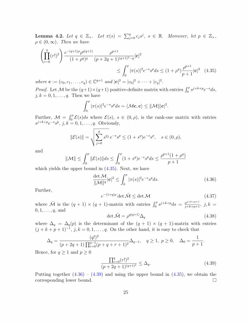
Lemma 4.2. Let q ∈ Z+. Let π(s) =∑q
j=0 cjsj, s ∈ R. Moreover, let p ∈ Z+,
ρ ∈ (0,∞). Then we have(
q∏
r=0
(r!)2
)e−(q+1)ρρq(q+1)
(1 + ρq)qρp+1
(p+ 2q + 1)(q+1)2−q |c|2
≤∫ ρ
0
|π(s)|2e−sspds ≤ (1 + ρq)ρp+1
p+ 1|c|2 (4.35)
where c := (c0, c1, . . . , cq) ∈ Cq+1 and |c|2 = |c0|2 + · · ·+ |cq|2.
Proof. LetM be the (q+1)×(q+1) positive-definite matrix with entries∫ ρ
0sj+k+pe−sds,
j, k = 0, 1, . . . , q. Then we have∫ ρ
0
|π(s)|2e−sspds = 〈Mc, c〉 ≤ ‖M‖|c|2.
Further, M =∫ ρ
0E(s)ds where E(s), s ∈ (0, ρ), is the rank-one matrix with entries
sj+k+pe−ssp, j, k = 0, 1, . . . , q. Obviously,
‖E(s)‖ =
√√√√q∑
j=0
s2j e−ssp ≤ (1 + sq)e−ssp, s ∈ (0, ρ),
and
‖M‖ ≤∫ ρ
0
‖E(s)‖ds ≤∫ ρ
0
(1 + sq)e−sspds ≤ ρp+1(1 + ρq)
p+ 1
which yields the upper bound in (4.35). Next, we have
detM‖M‖q |c|
2 ≤∫ ρ
0
|π(s)|2e−sspds. (4.36)
Further,e−(1+q)ρ detM ≤ detM (4.37)
where M is the (q + 1) × (q + 1)-matrix with entries∫ ρ
0sj+k+pds = ρj+k+p+1
j+k+p+1, j, k =
0, 1, . . . , q, anddetM = ρq(q+1)∆q (4.38)
where ∆q = ∆q(p) is the determinant of the (q + 1) × (q + 1)-matrix with entries(j + k + p+ 1)−1, j, k = 0, 1, . . . , q. On the other hand, it is easy to check that
∆q =(q!)2
(p+ 2q + 1)∏q−1
r=0(p+ q + r + 1)2∆q−1, q ≥ 1, p ≥ 0, ∆0 =
1
p+ 1.
Hence, for q ≥ 1 and p ≥ 0∏q
r=0(r!)2
(p+ 2q + 1)(q+1)2 ≤ ∆q. (4.39)
Putting together (4.36) – (4.39) and using the upper bound in (4.35), we obtain thecorresponding lower bound.
25

In the following proposition we obtain the needed lower bound of ratio (4.33).
Proposition 4.1. There exists a constant C > 0 such that for sufficiently large m andl ratio (4.33) satisfies the estimates
Rγ ≥ e−Cm ln l (4.40)
for each linear combination Pm of the form (4.34).
Proof. Evidently,
∫
|x−γ|≤ε|Pm(x)|2dx =
∫
|x|≤ε|Pm(x+ γ)|2dx =
∫
|x|≤ε|(τγPm)(x)|2, (4.41)
∫
|x|≤√
2l
|Pm(x)|2dx ≤∫
|x−γ|≤2√
2l
|Pm(x)|2 =
∫
|x|≤2√
2l
|Pm(x+ γ)|2dx =
∫
|x|≤2√
2l
|(τγPm)(x)|2dx, (4.42)
the magnetic translation operator τγ being defined in (2.6). Using the fact that τγcommutes with the the creation operator a∗ (see (3.30)), we easily find that (3.29)implies
(τγPm)(x) =m∑
j=0
cj(a∗)q(zjeζze−b|z|
2/4)
(4.43)
where z = x1 + ix2, ζ = − b2(γ1 − iγ2), and the coefficients cj, j = 0, 1, . . . ,m, may
depend on γ, b and q but are independent of x ∈ R2. Applying (3.26) and (3.29), weget
m∑
j=0
cj(a∗)q(zjeζze−b|z|
2/4)
=m∑
j=0
cj
∞∑
k=0
ζk
k!(a∗)q
(zj+ke−b|z|
2/4)
=
e−b|z|2/4
m∑
j=0
cjzj−q
∞∑
k=0
(ζz)k
k!L(j+k−q)q (b|z|2/2) (4.44)
with cj, j = 0, 1, . . . ,m, independent of x ∈ R2. By [9, Eq.(8.977.2)] we have
∞∑
k=0
(ζz)k
k!L(j+k−q)q (b|z|2/2) = eζzL(j−q)
q
(b|z|2
2− ζz
), (4.45)
while the Taylor expansion formula entails
L(j−q)q
(b|z|2
2− ζz
)=
q∑
s=0
(−ζz)s
s!
dsL(j−q)q (ξ)
dξs∣∣ξ=b|z|2/2
, (4.46)
26

and [9, Eq.(8.971.3)] yields
dsL(j−q)q (ξ)
dξs= (−1)sL
(j−q+s)q−s (ξ), ξ ∈ R. (4.47)
Combining (4.43) - (4.47), we find that
(τγPm)(x) = eζzPm(x), x ∈ R2, (4.48)
where
Pm(x) = e−b|z|2/4
m∑
j=0
cj
q∑
s=0
ζs
s!zj+s−qL(j+s−q)
q−s (b|z|2/2) =
e−b|z|2/4
m+q∑
p=0
zp−qφp,q(b|z|2/2), (4.49)
and φp,q, p = 0, . . . ,m + q, are polynomials of degree not exceeding q; moreover, ifp < q, then the minimal possible degree of the non-zero monomial terms in φp,q, is q−p.Bearing in mind that |eζz|2 = ex·γ and |γ| ≤
√2
2l, we find that there exists a constant C
such that for sufficiently large l we have
Rγ ≥ e−Cl2
R (4.50)
where
R =
∫|x|≤ε |Pm(x)|2dx
∫|x|≤2
√2l|Pm(x)|2dx
, (4.51)
the functions Pm being defined in (4.49). Passing to the polar coordinates (r, θ) inR2, after that changing the variable s = br2/2, and taking into account the rotationalsymmetry we find that for each R > 0 we have
∫
|x|≤R|Pm(x)|2dx =
2π
b
m+q∑
p=0
(2
b
)p−q ∫ ρ
0
sp−qe−s|φp,q(s)|2ds =
m∑
p=0
∫ ρ
0
spe−s|Πp,q(s)|2ds+
q∑
p=1
∫ ρ
0
spe−s|Πp,q(s)|2ds; (4.52)
if q = 0, then the second term in the last line of (4.52) should be set equal to zero. Here
ρ = bR2/2, Πp,q(s) =√
2πb
(2b
)pφp+q,q(s), p = 0, . . . ,m, Πp,q =
√2πb
(2b
)−ps−pφq−p,q(s),
p = 1, . . . , q. Note that the degree of the polynomials Πq,p does not exceed q, and thethe degree of the polynomials Πq,p does not exceed q − p. Bearing in mind (4.52) andapplying Lemma 4.2, we easily deduce the existence of a constant C > 0 such that forsufficiently large m and l we have
R ≥ e−Cm ln l,
which combined with (4.50) yields (4.40).
27

Next, we pick an arbitrary η and ν = ν(η), the number defined in Corollary 3.1. Further,we choose ς > 1 and δ ∈ (0, 1/2) so that ς (1− δ) > 1 + 2ν, and set
l = | lnE|δ/2, m ∼ ς| logE|log | logE| , L = (2n+ 1)a/2. (4.53)
Then, for E sufficiently small, (4.6) – (4.7) are satisfied. Further, we impose the addi-tional condition that µ := Cςδ
2< 1 where C is the constant in (4.40), which is compatible
with the conditions on ς and δ formulated above. Now, the probability that there existsγ ∈ 2lZ2∩Λ2L and a non identically vanishing function ψ in the span of {ej}0≤j≤m suchthat (4.8) be satisfied, is not greater than the probability that
l−2∑
|γ|≤lωγ ≤ l−2E1−µ = E1−µ| lnE|δ.
Arguing as in the derivation of (4.31) and (4.32), we conclude that for any θ ∈ T∗2L wehave
P(rq,m,ω has an eigenvalue less than E) ≤exp
(C8l
2 logP(ω0 ≤ E1−µ| lnE|δ)≤ exp
(−C9| lnE|1+δ ln | lnE|
)(4.54)
with positive C8 and C9 independent of θ and E > 0 small enough. Combining theupper bound in (3.39), (4.5), and (4.54), we get (4.3).This completes the proof of the upper bounds in Theorem 2.1.
5 Proof of Theorem 2.1: lower bounds of the IDS
In this section we get the lower bounds of Nb(2bq + E)−Nb(2bq) needed for the proofof Theorem 2.1.
Theorem 5.1. Assume that H1 – H4 hold, that almost surely ωγ ≥ 0, γ ∈ Z2, and(2.1) is valid. Fix the Landau level 2bq, q ∈ Z+.i) We have
lim infE↓0
ln | ln (Nb(2bq + E)−Nb(2bq))|| lnE| ≤ 2
κ − 2, (5.1)
where κ is the constant in (1.2).ii) Let u(x) ≤ e−C|x|
β, x ∈ R2, for some C > 0 and β ∈ (0, 2]. Then we have
lim supE↓0
ln (Nb(2bq + E)−Nb(2bq))| lnE|1+2/β
≥ −πκC, (5.2)
if β ∈ (0, 2), and
lim infE↓0
ln (Nb(2bq + E)−Nb(2bq))| lnE|2 ≥ −πκ
(2
b+
1
C
), (5.3)
28

if β = 2. Therefore,
lim supE↓0
ln | ln (Nb(2bq + E)−Nb(2bq))|ln | lnE| ≤ 1 + 2/β. (5.4)
Note that the combination of Theorem 4.1 with Theorem 5.1 completes the proof ofTheorem 2.1.Let us prove now Theorem 5.1. Pick η ≥ 2
κ−2in the case of its first part, or an arbitrary
η > 0 in the case of its second part. As above, set n ∼ E−ν where ν = ν(η) is thenumber defined in Corollary 3.1, and L = (2n + 1)a/2. Bearing in mind the lowerbound in (3.39), and (4.4), we conclude that it suffices to estimate from below thequantity
E (ρq,n,ω(E)) =1
(2π)2
∫
Λ∗2L
E(N(E; rq,n,ω(θ))dθ
= (2π)−2
∫
Λ∗2L
rank rq,n,ω(θ)∑
j=1
P(λj(θ) < E)dθ
≥ (2π)−2
∫
Λ∗2L
P(λ1(θ) < E)dθ.
(5.5)
Fix an arbitrary θ ∈ T∗2L. Evidently, P(λ1(θ) < E) is equal to the probability that thereexists a non-zero function f ∈ Ran rq,n,ω(θ) such that
∫
Λ2L
Vω(x)|f(x; θ)|2dx < E
∫
Λ2L
|f(x; θ)|2dx. (5.6)
Further, pick the trial function
ϕ(x; θ) =∑
γ∈2LZ2
e−iθ(x+γ)(τγϕ)(x), x ∈ Λ2L, θ ∈ T∗2L, (5.7)
whereϕ(x) = ϕq(x) := zqe−b|z|
2/4, z = x1 + ix2, z = x1 − ix2. (5.8)
Since the function ϕq is proportional to e0,q (see (3.26)), we have ϕ ∈ Ran rq,n,ω(θ).Therefore, the probability that there exists a non-zero function f ∈ Ran rq,n,ω(θ) suchthat (5.6) holds, is not less than the probability that
∫
Λ2L
Vω(x)|ϕ(x; θ)|2dx < E
∫
Λ2L
|ϕ(x; θ)|2dx. (5.9)
Lemma 5.1. Let the function ϕ be defined as in (5.7) – (5.8). Then there exist L0 > 0and c1 > 0 independent of θ such that L ≥ L0 implies
∫
Λ2L
|ϕ(x; θ)|2dx > c1. (5.10)
29

Proof. We have ϕ = ϕ0 + ϕ∞ where
ϕ0(x; θ) = e−iθxϕ(x), (5.11)
ϕ∞(x; θ) =∑
γ∈2LZ2, γ 6=0
e−iθ(x+γ)(τγϕ)(x). (5.12)
Note thatsupx∈Λ2L
|ϕ∞(x; θ)| ≤ ce−cL2
(5.13)
with c independent of L and θ. Further,
∫
Λ2L
|ϕ(x; θ)|2dx ≥ 1
2
∫
Λ2L
|ϕ0(x; θ)|2dx− 2
∫
Λ2L
|ϕ∞(x; θ)|2dx
≥ 1
2
∫
R2
|ϕ(x)|2dx− 8cL2e−cL2
.
(5.14)
Taking into account that∫R2 |ϕ|2dx = 2π
b
(2q
)qq!, we find that (5.14) implies (5.10).
By assumption we have
u(x) ≤ Cv(x), C > 0, x ∈ R2, (5.15)
where v(x) := (1 + |x|)−κ in the case of Theorem 5.1 i), and v(x) := e−C|x|β
in the caseof Theorem 5.1 ii). Since ωγ ≥ 0, inequality (5.9) will follow from
∑
γ∈Z2
ωγ
∫
Λ2L
v(x− γ)|ϕ(x; θ)|2dx ≤ c2E (5.16)
where c2 = c1C−1, C being the constant in (5.15), and c1 being the constant in (5.10).
Next, we write ∑
γ∈Z2
ωγ
∫
Λ2L
v(x− γ)|ϕ(x; θ)|2dx ≤
2∑
γ∈Z2
ωγ
∫
Λ2L
v(x− γ)|ϕ0(x; θ)|2dx+ 2∑
γ∈Z2
ωγ
∫
Λ2L
v(x− γ)|ϕ∞(x; θ)|2dx (5.17)
where ϕ0 and ϕ∞ are defined in (5.11) and (5.12) respectively.
Lemma 5.2. Fix q ∈ Z+.i) Let κ > 0, b > 0. Then there exists a constant c′ > 0 such that for each y ∈ R2,L > 0, and θ ∈ T∗2L, we have
∫
Λ2L
(1 + |x− y|)−κ|ϕ0(x; θ)|2dx ≤ c′(1 + |y|)−κ. (5.18)
30

ii) Let β ∈ (0, 2], b > 0, C > 0. If β ∈ (0, 2), set b0 := C. If β = 2, set b0 := Cb2C+b
.Then for each b1 < b0 there exists a constant c′′ > 0 such that for each y ∈ R2, L > 0,and θ ∈ T∗2L, we have
∫
Λ2L
e−C|x−y|β |ϕ0(x; θ)|2dx ≤ c′′e−b1|y|
β
. (5.19)
We omit the proof since estimates (5.18) – (5.19) follow from standard simple factsconcerning the asymptotics at infinity of the convolutions of functions admitting power-like or exponential decay, with the derivatives of Gaussian functions. In the case ofpower-like decay, results of this type can be found in in [34, Theorem 24.1], and in thecase of an exponential decay similar results are contained in [12, Lemma 3.5].Using Lemma 5.2, we find that under the hypotheses of Theorem 5.1 i) we have
2∑
γ∈Z2
ωγ
∫
Λ2L
v(x− γ)|ϕ0(x; θ)|2dx ≤ c3
∑
γ∈Z2
ωγ(1 + γ|)−κ, (5.20)
while under the hypotheses of Theorem 5.1 ii) for each b1 < b0 we have
2∑
γ∈Z2
ωγ
∫
Λ2L
v(x− γ)|ϕ0(x; θ)|2dx ≤ c3
∑
γ∈Z2
ωγe−b1|γ|2, (5.21)
where c3 is independent of L and θ. Further, for both parts of Theorem 5.1 we have
2∑
γ∈Z2
ωγ
∫
Λ2L
v(x− γ)|ϕ∞(x; θ)|2dx ≤ c4L2e−cL
2
(5.22)
where c4 is independent of L and θ, and c is the constant in (5.13). Since L ∼ E−ν ,ν > 0, we have
c2E − c4L2e−cL
2 ≥ c2
2E (5.23)
for sufficiently small E > 0. Combining (5.17) with (5.20) – (5.23), and setting c5 =c2/(2c3), we find that (5.16) will follow from the inequality
∑
γ∈Z2
ωγc5(1 + |γ|)−κ ≤ c5E, (5.24)
in the case of Theorem 5.1 i), or from the inequality
∑
γ∈Z2
ωγe−b1|γ|β ≤ c5E, b1 < b0, (5.25)
in the case of Theorem 5.1 ii). Now pick l > 0 and write
∑
γ∈Z2
ωγ(1 + |γ|)−κ ≤∑
γ∈Z2, |γ|≤lωγ +
∑
γ∈Z2, |γ|>lωγ|γ|−κ, (5.26)
31

∑
γ∈Z2
ωγe−b1|γ|β ≤
∑
γ∈Z2, |γ|≤lωγ +
∑
γ∈Z2, |γ|>lωγe
−b1|γ|β . (5.27)
Evidently, for each κ′ ∈ (2,κ) and b2 < b1 there exists a constant c6 > 0 such that
∑
γ∈Z2, |γ|>lωγ|γ|−κ ≤ c6l
−κ′+2, (5.28)
∑
γ∈Z2, |γ|>lωγe
−b1|γ|β ≤ c6e−b2lβ . (5.29)
Fix l and c7 ∈ (0, c5) such that
l−κ′+2 =
c5 − c7
c6
E (5.30)
in the case of Theorem 5.1 i), or
e−b2lβ
=c5 − c7
c6
E (5.31)
in the case of Theorem 5.1 ii). Putting together (5.26) - (5.31), we conclude that (5.24),or, respectively, (5.25) will follow from the inequality
∑
γ∈Z2, |γ|≤lωγ ≤ c7E (5.32)
provided that l satisfies (5.30) or, respectively, (5.31). Set
N(l) := #{γ ∈ Z2 ; |γ| ≤ l},
so that we haveN(l) = πl2(1 + o(1)), l→∞. (5.33)
Evidently, the probability that (5.32) holds, is not less than the probability that ωγ ≤c7E/N(l) for each γ ∈ Z2 such that |γ| ≤ l. Since the random variables ωγ are identicallydistributed and independent, the last probability is equal to P(ω0 ≤ c7E/N(l))N(l).Combining the above inequalities, and using the lower bound in (3.39), we get
Nb(2bq + E)−Nb(2bq) ≥area Λ∗2L
(2π)2P(ω0 ≤ c7E/N(l))N(l) − e−E−η , (5.34)
where l is chosen to satisfy (5.30) with an arbitrary κ′ ∈ (2,κ) in the case of Theorem5.1 i), or to satisfy (5.31) with an arbitrary fixed b2 < b0 in the case of Theorem 5.1 ii).Putting together (5.34), (2.1), (5.30), and (5.33), we get
lim supE↓0
ln | ln (Nb(2bq + E)−Nb(2bq))|| lnE| ≤ 2
κ′ − 2
32

for any κ′ ∈ (2,κ) such that η > 2κ′−2
. Letting κ′ ↑ κ, we get (5.1).Similarly, putting together (5.34), (2.1), (5.31), and (5.33), we get
lim infE↓0
ln (Nb(2bq + E)−Nb(2bq))| lnE|1+ 1
β
≥ −πκb2
for any b2 < b0. Letting
b2 ↑ b0 =
{1C
if β ∈ (0, 2),bCb+2C
if β = 2,
we get (5.2) – (5.3).
Acknowledgments. The financial support of the Chilean Science Foundation Fondecytunder Grants 1020737 and 7020737 is acknowledged by both authors. Georgi Raikovis sincerely grateful for the warm hospitality of his colleagues at the Department ofMathematics, University of Paris 13, during his visit in 2004, when a considerable partof this work was done. He would like to thank also Werner Kirsch, Hajo Leschke andSimone Warzel for several illuminating discussions.
References
[1] J. Avron, I. Herbst, B. Simon, Schrodinger operators with magnetic fields. I. Generalinteractions, Duke. Math. J. 45 (1978), 847-883.
[2] K. Broderix, D. Hundertmark, W. Kirsch, H. Leschke, The fate of Lifshits tailsin magnetic fields, J. Statist. Phys. 80 (1995), 1–22.
[3] V. Bruneau, A. Pushnitski, G. D. Raikov, Spectral shift function in strong magneticfields, Algebra i Analiz 16 (2004), 207-238.
[4] M. Dimassi, J. Sjostrand, Spectral Asymptotics in the Semi-Classical Limit. LondonMathematical Society Lecture Notice Series 268 Cambridge University Press, 1999.
[5] B. A. Dubrovin, S. P. Novikov, Ground states in a periodic field. Magnetic Blochfunctions and vector bundles, Sov. Math., Dokl. 22 (1980), 240-244.
[6] L. Erdos, Lifschitz tail in a magnetic field: the nonclassical regime, Probab. TheoryRelated Fields 112 (1998), 321–371.
[7] L. Erdos, Lifschitz tail in a magnetic field: coexistence of classical and quantum behaviorin the borderline case, Probab. Theory Related Fields 121 (2001), 219–236.
[8] V.Fock, Bemerkung zur Quantelung des harmonischen Oszillators im Magnetfeld, Z.Physik 47 (1928), 446-448.
[9] I. S. Gradshteyn, I. M. Ryzhik, Table of Integrals, Series, and Products, New YorkSan Francisco, London, 1965.
33

[10] B. Helffer, J. Sjostrand, Equation de Schrodinger avec champ magnetique etequation de Harper, In: H. Holden and A. Jensen (eds.), Schrodinger operators, Pro-ceedings, Sonderborg, Denmark 1988, Lect.Notes in Physics 345 (1988), 118-197.
[11] T. Hupfer, H. Leschke, P. Muller, S. Warzel, Existence and uniqueness of theintegrated density of states for Schrodinger operators with magnetic fields and unboundedrandom potentials, Rev. Math. Phys. 13 (2001), 1547–1581.
[12] T.Hupfer, H.Leschke, S.Warzel, Poissonian obstacles with Gaussian walls discrim-inate between classical and quantum Lifshits tailing in magnetic fields, J. Statist. Phys.97 (1999), 725–750.
[13] T.Hupfer, H.Leschke, S.Warzel, The multiformity of Lifshits tails caused by randomLandau Hamiltonians with repulsive impurity potentials of different decay at infinity,In: Differential equations and mathematical physics (Birmingham, AL, 1999), 233–247,AMS/IP Stud. Adv. Math., 16, Amer. Math. Soc., Providence, RI, 2000.
[14] T.Hupfer, H.Leschke, S.Warzel, Upper bounds on the density of states of singleLandau levels broadened by Gaussian random potentials, J. Math. Phys. 42 (2001), 5626-5641.
[15] W. Kirsch, Random Schrodinger operators: a course. In: Schrodinger operators, Proc.Nord. Summer Sch. Math., Sandbjerg Slot, Soenderborg/Denmark 1988, Lect. NotesPhys. 345, Springer, Berlin, (1989) 264-370.
[16] W. Kirsch, F. Martinelli, On the spectrum of Schrodinger operators with a randompotential, Comm. Math. Phys. 85 (1982), 329–350.
[17] W. Kirsch, F. Martinelli, Large deviations and Lifshitz singularity of the integrateddensity of states of random Hamiltonians, Comm. Math. Phys. 89 (1983), 27–40.
[18] W. Kirsch, B. Simon, Lifshitz tails for periodic plus random potentials, J. Statist.Phys. 42 (1986), no. 5-6, 799–808.
[19] W. Kirsch, B. Simon, Comparison theorems for the gap of Schrodinger operators, J.Funct. Anal. 75 (1987), 396–410.
[20] F. Klopp, An asymptotic expansion for the density of states of a random Schrodingeroperator with Bernoulli disorder, Random Oper. Stochastic Equations 3 (1995), 315–331.
[21] F. Klopp, Internal Lifshits tails for random perturbations of periodic Schrodinger op-erators, Duke Math. J. 98 (1999), 335–396.
[22] F. Klopp, Lifshitz tails for random perturbations of periodic Schrodinger operators, In:Spectral and inverse spectral theory (Goa, 2000). Proc. Indian Acad. Sci. Math. Sci. 112(2002), 147–162.
[23] F. Klopp, L. Pastur, Lifshitz tails for random Schrodinger operators with negativesingular Poisson potential, Comm. Math. Phys. 206 (1999), 57–103.
[24] F. Klopp, J. Ralston, Endpoints of the spectrum of periodic operators are genericallysimple, In: Cathleen Morawetz: a great mathematician. Methods Appl. Anal. 7 (2000),459–463.
[25] F. Klopp, T. Wolff, Lifshitz tails for 2-dimensional random Schrodinger operators.Dedicated to the memory of Tom Wolff, J. Anal. Math. 88 (2002), 63–147.
34

[26] L. Landau, Diamagnetismus der Metalle, Z. Physik 64 (1930), 629-637.
[27] J. N. Mather, On Nirenberg’s proof of Malgrange’s preparation theorem, In: Proceed-ings of Liverpool Singularities—Symposium, I (1969/70), pp. 116–120. Lecture Notes inMathematics, 192 Springer, Berlin, 1971.
[28] G. Mezincescu, Lifschitz singularities for periodic operators plus random potentials, J.Statist. Phys. 49 (1987), 1181–1190.
[29] G. Mezincescu, Internal Lifshitz singularities for one-dimensional Schrodinger opera-tors, Commun.Math.Phys. 158 (1993), 315-325.
[30] A. Mohamed, G. Raikov, On the spectral theory of the Schrodinger operator withelectromagnetic potential, Pseudo-differential calculus and mathematical physics, 298–390, Math. Top., 5, Akademie Verlag, Berlin, 1994.
[31] L.Pastur, A.Figotin, Spectra of Random and Almost-Periodic Operators.Grundlehren der Mathematischen Wissenschaften 297, Springer-Verlag, Berlin,1992.
[32] G.D.Raikov, S.Warzel, Quasi-classical versus non-classical spectral asymptotics formagnetic Schrodinger operators with decreasing electric potentials, Rev. Math. Phys. 14(2002), 1051–1072.
[33] M.Reed, B.Simon, Methods of Modern Mathematical Physics. IV. Analysis of Opera-tors, Academic Press, New York, 1978.
[34] M.A.Shubin, Pseudodifferential Operators and Spectral Theory, Second Edition,Springer-Verlag, Berlin, 2001.
[35] J. Sjostrand, Microlocal analysis for the periodic magnetic Schrodinger equation andrelated questions, IN: Microlocal analysis and applications (Montecatini Terme, 1989),237–332, Lecture Notes in Math., 1495, Springer, Berlin, 1991.
[36] I. Veselic, Integrated density of states and Wegner estimates for random Schrodingeroperators, Spectral Theory of Schrodinger Operators, 97–183, Contemp. Math. 340,AMS, Providence, RI, 2004.
Frederic KloppDepartement de mathematiquesUniversite de Paris NordAvenue J. Baptiste Clement93430 Villetaneuse, FranceE-mail: [email protected]
Georgi RaikovDepartamento de MatematicasFacultad de CienciasUniversidad de ChileLas Palmeras 3425Santiago, ChileE-mail: [email protected]
35