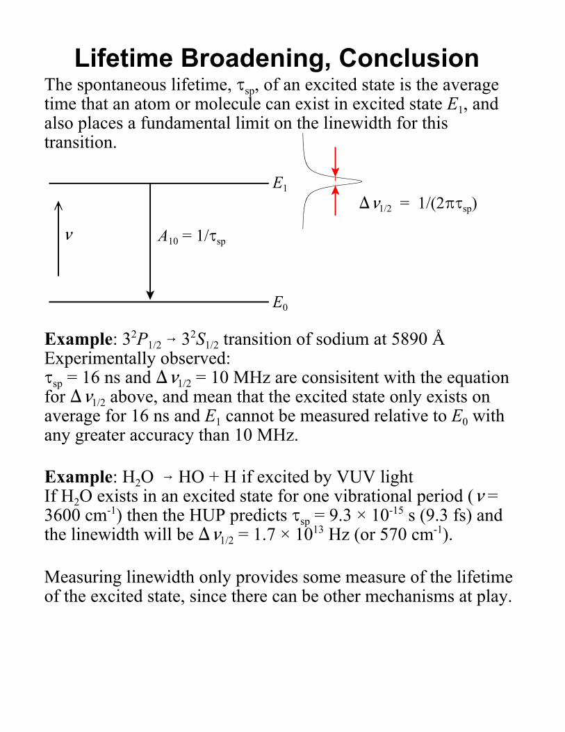
Lifetime Broadening, ConclusionThe spontaneous lifetime, Jsp, of an excited state is the averagetime that an atom or molecule can exist in excited state E1, andalso places a fundamental limit on the linewidth for thistransition.

< A10 = 1/Jsp

E1

E0

)<1/2 = 1/(2BJsp)

Example: 32P1/2 6 32S1/2 transition of sodium at 5890 ÅExperimentally observed: Jsp = 16 ns and )<1/2 = 10 MHz are consisitent with the equationfor )<1/2 above, and mean that the excited state only exists onaverage for 16 ns and E1 cannot be measured relative to E0 withany greater accuracy than 10 MHz.

Example: H2O 6 HO + H if excited by VUV lightIf H2O exists in an excited state for one vibrational period (< =3600 cm-1) then the HUP predicts Jsp = 9.3 × 10-15 s (9.3 fs) andthe linewidth will be )<1/2 = 1.7 × 1013 Hz (or 570 cm-1).

Measuring linewidth only provides some measure of the lifetimeof the excited state, since there can be other mechanisms at play.

Pressure BroadeningPressure broadening results from collisions of molecules, anddepends on their intermolecular potentials. Since moleculescollide with one another, there is an exchange of energy whicheffectively broadens or “blurs” the energy levels. The dipolemoment oscillates at the Bohr frequency - but the phase israndomly altered if collisions occur.

)<1/2 ' (2BJc)&1

where b is the pressure-broadening coefficient, and isexperimentally measured (e.g., 10 MHz Torr-1 is a typical value)

Mt

The infinitely sharp lineshape associated with a perfectlyoscillating cos wave now takes on a finite width. If Jc is theaverage time between collisions, and each collision results in atransition between two states, there is a broadening, )<, of thetransition where

This is the result of FT of autocorrelation functions, and canalso be derived from the uncertainty principle. The average timebetween collisions is proportional to the inverse of the pressure

)<1/2 ' bp

Pressure broadening results in homogeneous Lorentzianlineshapes similar to lifetime broadening.

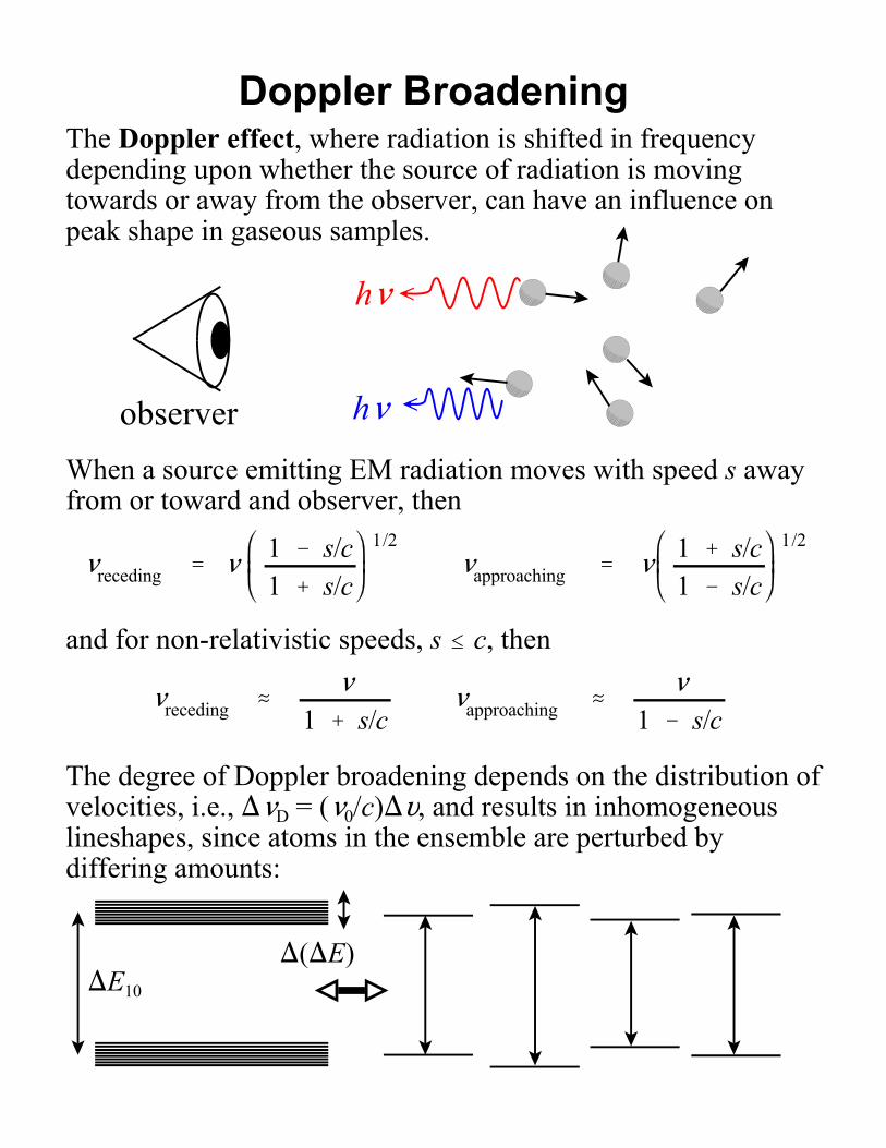
Doppler BroadeningThe Doppler effect, where radiation is shifted in frequencydepending upon whether the source of radiation is movingtowards or away from the observer, can have an influence onpeak shape in gaseous samples.

h<

h<

observerWhen a source emitting EM radiation moves with speed s awayfrom or toward and observer, then

<receding ' <1 & s/c1 % s/c

1/2<approaching ' <

1 % s/c1 & s/c

1/2

and for non-relativistic speeds, s # c, then

<receding . <

1 % s/c<approaching . <

1 & s/c

The degree of Doppler broadening depends on the distribution ofvelocities, i.e., )<D = (<0/c))L, and results in inhomogeneouslineshapes, since atoms in the ensemble are perturbed bydiffering amounts:

)E10

)()E)

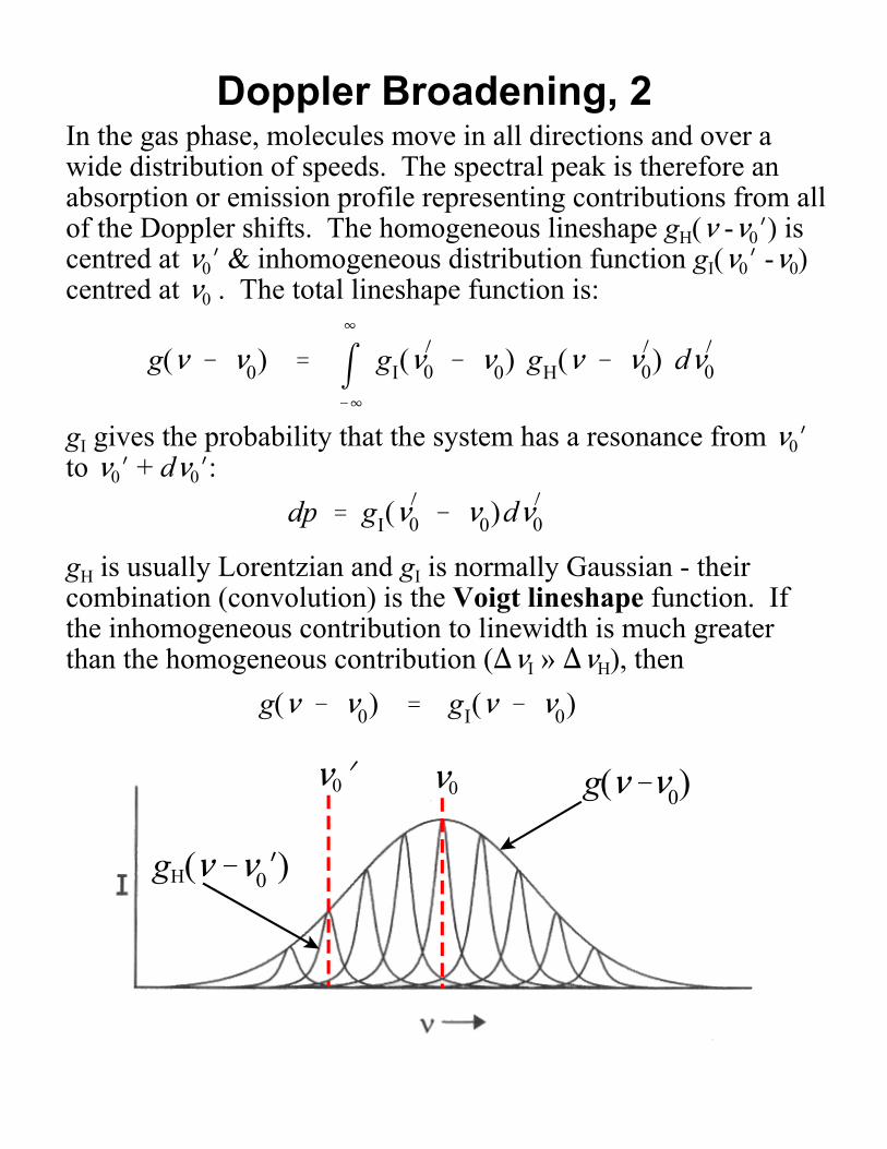
Doppler Broadening, 2In the gas phase, molecules move in all directions and over awide distribution of speeds. The spectral peak is therefore anabsorption or emission profile representing contributions from allof the Doppler shifts. The homogeneous lineshape gH(< -<0N) iscentred at <0N & inhomogeneous distribution function gI(<0N -<0)centred at <0 . The total lineshape function is:

g(< & <0) ' m4

&4

gI(<)

0 & <0) gH(< & <)

0) d<)0

gI gives the probability that the system has a resonance from <0Nto <0N + d<0N:

dp ' gI(<)

0 & <0)d<)0gH is usually Lorentzian and gI is normally Gaussian - theircombination (convolution) is the Voigt lineshape function. Ifthe inhomogeneous contribution to linewidth is much greaterthan the homogeneous contribution ()<I » )<H), then

g(< & <0) ' gI(< & <0)

g(<&<0)

gH(<&<0N)

<0<0N

Doppler Broadening, 3If an atom of velocity v interacts with a parallel plane wave k,then the atom sees a Doppler shifted frequency <N = <(1 ± L/c) (-ve if same direction or +ve if opposite direction to EMradiation). Only the component of v along k is important, so

<) ' < 1 &v @ kc|k|

where *k* is the norm of the unit vector, and v·k = Lkcos2 = L

In the lab frame, the EM wave is at <, but the atomic resonancefrequency, <0 (which is moving at velocity L) is shifted to

<)

0 '<0

1 ± L/c

or more generally, an atom with velocity component Lz towardsan observer has a shifted frequency:

< ' <0 %Lx

c<0

The Maxwell-Boltzmann velocity distribution along a Cartesianaxis is given by

f(L) dL 'm

2BkT

1/2e &mL2 / (2kT) dL

Given that dL = (c/<0)d<0 (from differentiating (*) above), then

(*)

gD(< & <0) '1<0

mc 2

2BkT

1/2

e &mc 2(<&<20) / (2kT<20)

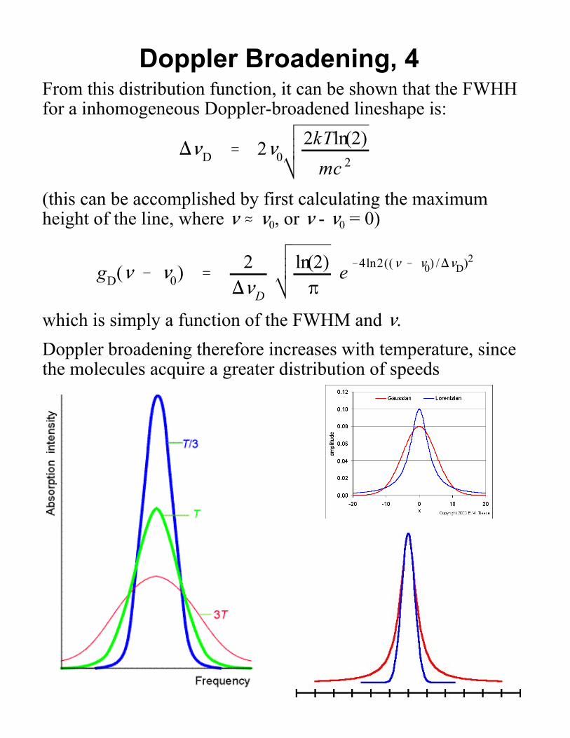
Doppler Broadening, 4From this distribution function, it can be shown that the FWHHfor a inhomogeneous Doppler-broadened lineshape is:

)<D ' 2<02kTln(2)

mc 2

(this can be accomplished by first calculating the maximumheight of the line, where < . <0, or < - <0 = 0)

which is simply a function of the FWHM and <.

gD(< & <0) '2)<D

ln(2)B

e &4ln2((< & <0) /)<D)2

Doppler broadening therefore increases with temperature, sincethe molecules acquire a greater distribution of speeds

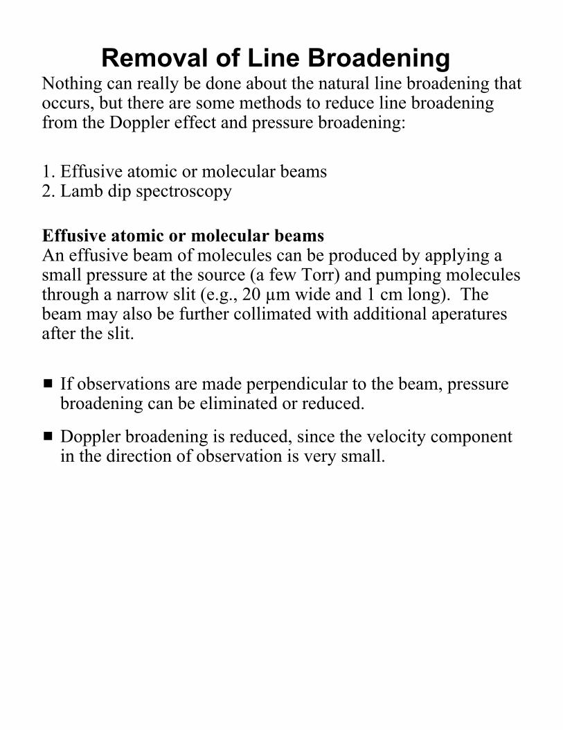
Removal of Line BroadeningNothing can really be done about the natural line broadening thatoccurs, but there are some methods to reduce line broadeningfrom the Doppler effect and pressure broadening:

1. Effusive atomic or molecular beams2. Lamb dip spectroscopy

Effusive atomic or molecular beamsAn effusive beam of molecules can be produced by applying asmall pressure at the source (a few Torr) and pumping moleculesthrough a narrow slit (e.g., 20 µm wide and 1 cm long). Thebeam may also be further collimated with additional aperaturesafter the slit.

# If observations are made perpendicular to the beam, pressurebroadening can be eliminated or reduced.

# Doppler broadening is reduced, since the velocity componentin the direction of observation is very small.

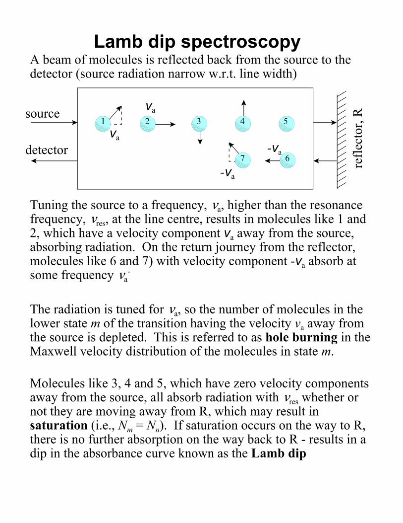
Lamb dip spectroscopyA beam of molecules is reflected back from the source to thedetector (source radiation narrow w.r.t. line width)

va

-va

source

detector

Tuning the source to a frequency, <a, higher than the resonancefrequency, <res, at the line centre, results in molecules like 1 and2, which have a velocity component va away from the source,absorbing radiation. On the return journey from the reflector,molecules like 6 and 7) with velocity component -va absorb atsome frequency <a

-

1 2 3 4 5

67

The radiation is tuned for <a, so the number of molecules in thelower state m of the transition having the velocity va away fromthe source is depleted. This is referred to as hole burning in theMaxwell velocity distribution of the molecules in state m.

Molecules like 3, 4 and 5, which have zero velocity componentsaway from the source, all absorb radiation with <res whether ornot they are moving away from R, which may result insaturation (i.e., Nm = Nn). If saturation occurs on the way to R,there is no further absorption on the way back to R - results in adip in the absorbance curve known as the Lamb dip

va

-va

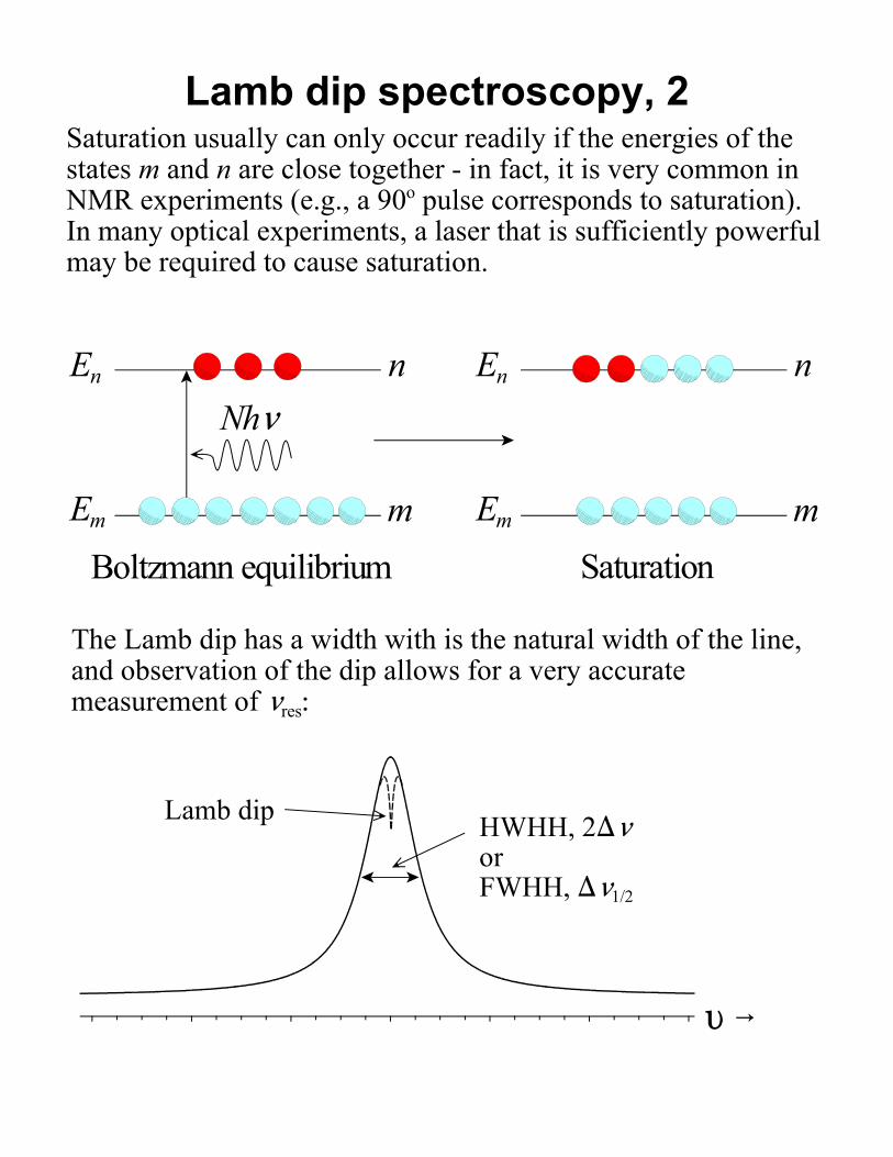
Lamb dip spectroscopy, 2Saturation usually can only occur readily if the energies of thestates m and n are close together - in fact, it is very common inNMR experiments (e.g., a 90o pulse corresponds to saturation). In many optical experiments, a laser that is sufficiently powerfulmay be required to cause saturation.

m

nEn

Em m

nEn

Em

Nh<

Boltzmann equilibrium Saturation

The Lamb dip has a width with is the natural width of the line,and observation of the dip allows for a very accuratemeasurement of <res:

L 6

HWHH, 2)<or FWHH, )<1/2

Lamb dip

Power BroadeningLasers find use in almost all areas of spectroscopy - interestingly,the intense EM radiation from lasers actually sometimes causebroadening and even splitting of lines. A simple estimate oflinewidth comes from

)E)t $ £

At very high powers, the system undergoes Rabi oscillations atTR = µ10E/£, and therefore, the system is only in the excited E1state for a period of ca. h/µ10E. Thus:

)E hµ10E

. £

or if h)< = )E, an uncertainty in frequency of

)< .µ10E2B£

'TR

4B2

Example:A 1 W laser beam of 1 mm diameter interacts with a two-levelsystem with a transition dipole moment of 1 D and TR = 9.8 × 108

rad s-1 gives )< = 25 MHz.

Pulsed lasers of 1 MW capacity (10 mJ in 10 ns) will increase Eto 3.1 × 107 V m-1 (by a factor of 1000 times!) compared to thefirst example, meaning that the linewidth is around 25000 MHzor 0.83 cm-1, exceeding typical Doppler widths.

N.B.: the E on its own symbolizes electric field in V m-1, and thedipole moments are given in Debye (1 D = 3.33564 × 10-30 C m)

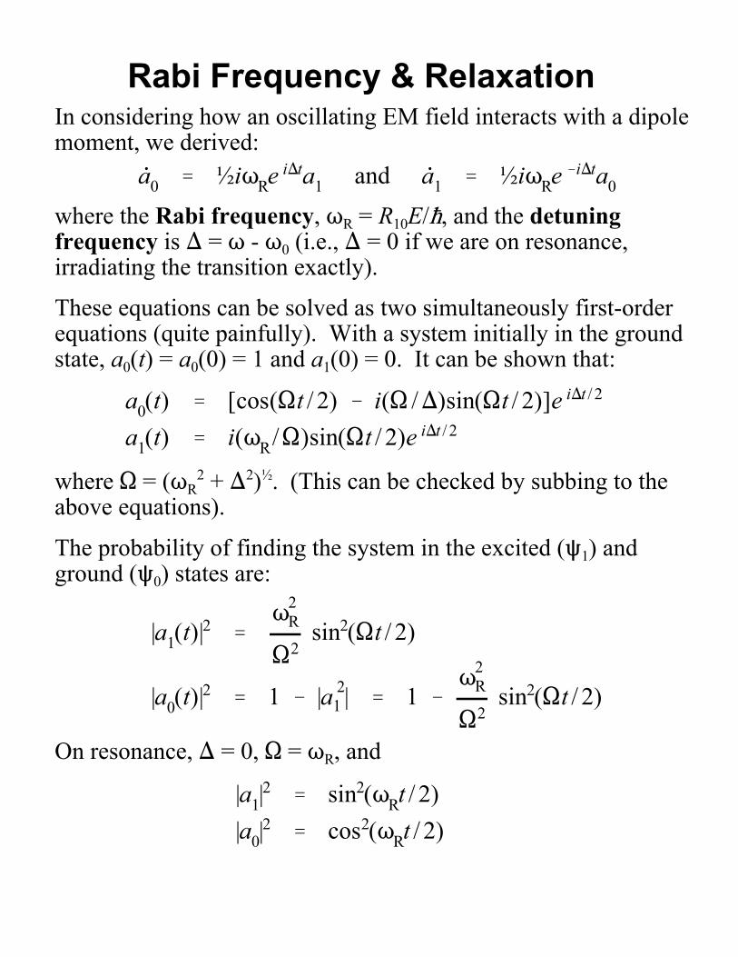
Rabi Frequency & RelaxationIn considering how an oscillating EM field interacts with a dipolemoment, we derived:

0a0 ' ½iTRe i)ta1 and 0a1 ' ½iTRe &i)ta0

where the Rabi frequency, TR = R10E/£, and the detuningfrequency is ) = T - T0 (i.e., ) = 0 if we are on resonance,irradiating the transition exactly).

These equations can be solved as two simultaneously first-orderequations (quite painfully). With a system initially in the groundstate, a0(t) = a0(0) = 1 and a1(0) = 0. It can be shown that:

a0(t) ' [cos(St / 2) & i(S /))sin(St / 2)]e i)t / 2

a1(t) ' i(TR/S)sin(St / 2)e i)t / 2

where S = (TR2 + )2)½. (This can be checked by subbing to the

above equations).

The probability of finding the system in the excited (R1) andground (R0) states are:

|a1(t)|2 '

T2R

S2sin2(St / 2)

|a0(t)|2 ' 1 & |a 2

1 | ' 1 &T

2R

S2sin2(St / 2)

On resonance, ) = 0, S = TR, and

|a1|2 ' sin2(TRt / 2)

|a0|2 ' cos2(TRt / 2)

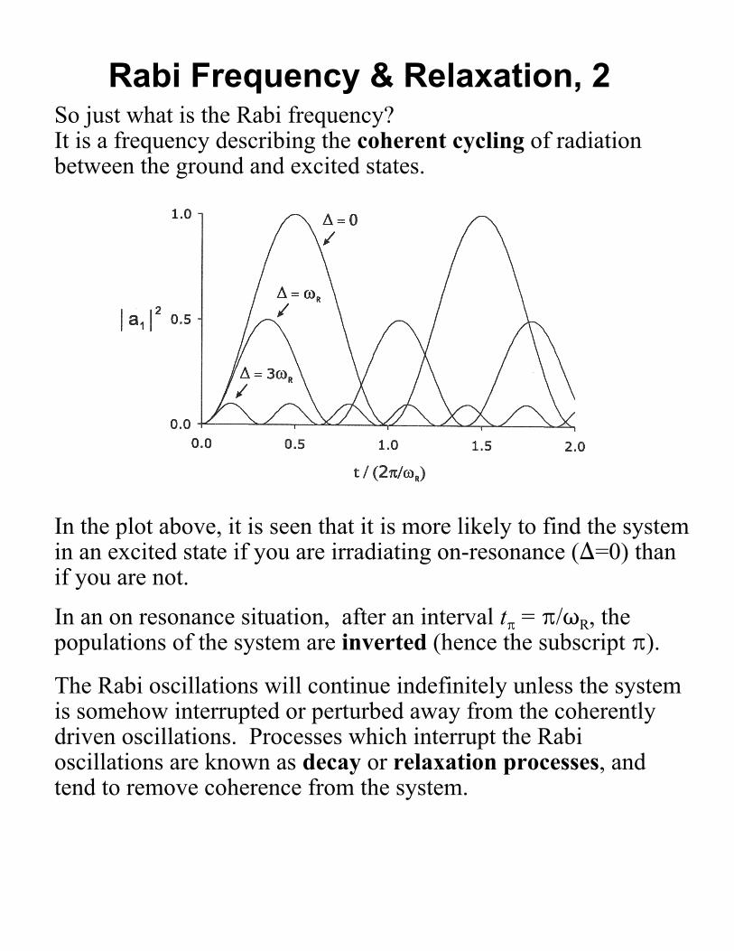
So just what is the Rabi frequency?It is a frequency describing the coherent cycling of radiationbetween the ground and excited states.

Rabi Frequency & Relaxation, 2

In the plot above, it is seen that it is more likely to find the systemin an excited state if you are irradiating on-resonance ()=0) thanif you are not.

The Rabi oscillations will continue indefinitely unless the systemis somehow interrupted or perturbed away from the coherentlydriven oscillations. Processes which interrupt the Rabioscillations are known as decay or relaxation processes, andtend to remove coherence from the system.

In an on resonance situation, after an interval tB = B/TR, thepopulations of the system are inverted (hence the subscript B).

The two general relaxation processes are termed T1 and T2, whichare also the rate constant names used to describe these processes.

Rabi Frequency & Relaxation, 3

T1 process: I0(1 - exp(-t/T1))Spontaneous emission breaks the coherence, returns the system tothe ground state (i.e., returns to thermal equilibrium populationspredicted by the Boltzmann distribution

T2 process: I0(exp(-t/T2))Collisions which result in changes in the phases of R1 and/or R0,but no change in the populations. The coherent cycling isinterrupted (as discussed earlier in pressure broadening). Theeffect of the T2 process is to dampen the Rabi oscillations.

In order to quench the effects of damping, one must increase theamplitude of the applied electric field, E, such that TR » Trelax. InNMR experiments, this is trivial; however, for IR and visiblerange processes, Rabi oscillations are always damped.

A system oscillates briefly when a strong E is applied, then losescoherence and becomes saturated (i.e., N1 = N0).

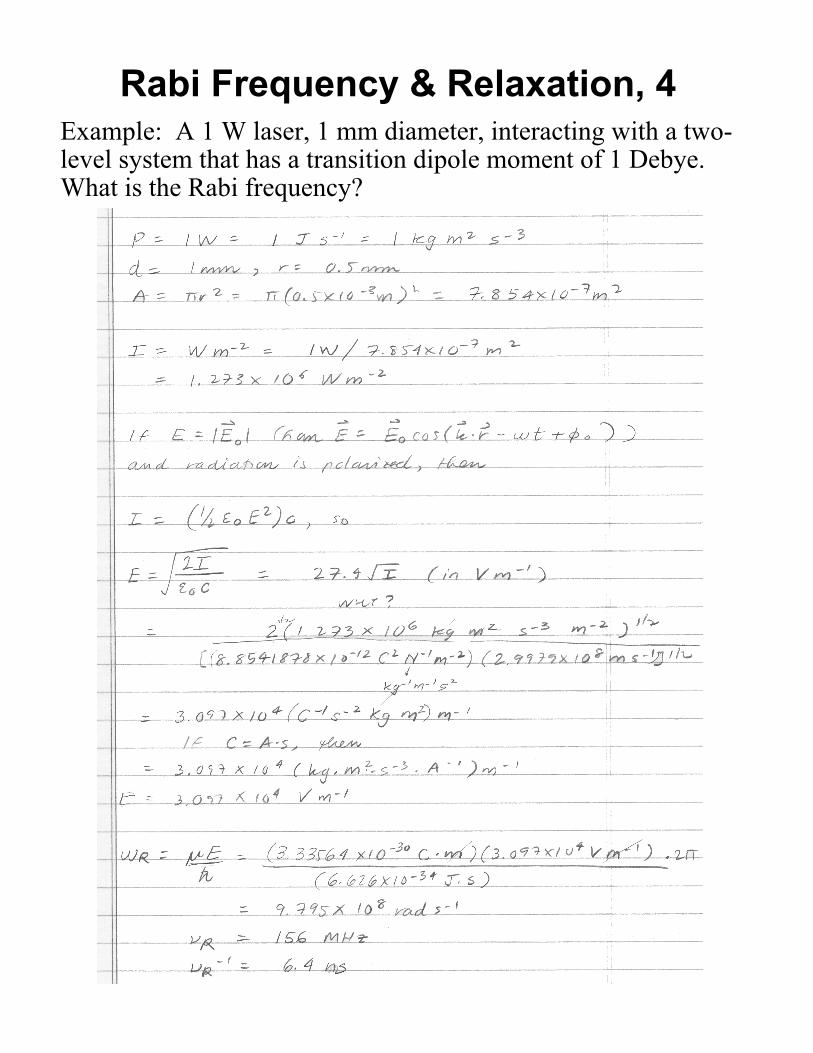
Example: A 1 W laser, 1 mm diameter, interacting with a two-level system that has a transition dipole moment of 1 Debye. What is the Rabi frequency?

Rabi Frequency & Relaxation, 4

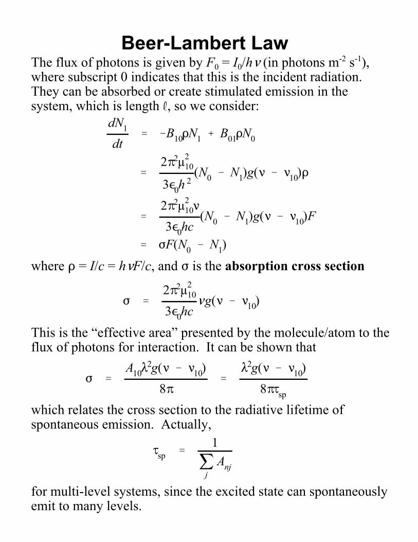
Beer-Lambert LawThe flux of photons is given by F0 = I0/h< (in photons m-2 s-1),where subscript 0 indicates that this is the incident radiation. They can be absorbed or create stimulated emission in thesystem, which is length R, so we consider:

dN1

dt' &B10DN1 % B01DN0

'2B2µ2

10

3,0h2

(N0 & N1)g(< & <10)D

'2B2µ2

10<

3,0hc(N0 & N1)g(< & <10)F

' FF(N0 & N1)

F '2B2µ2

10

3,0hc<g(< & <10)

F 'A108

2g(< & <10)8B

'82g(< & <10)

8BJsp

where D = I/c = h<F/c, and F is the absorption cross section

This is the “effective area” presented by the molecule/atom to theflux of photons for interaction. It can be shown that

which relates the cross section to the radiative lifetime ofspontaneous emission. Actually,

Jsp '1

jj

Anj

for multi-level systems, since the excited state can spontaneouslyemit to many levels.

If the flux is incident to an element of small thickness dx with across sectional area of 1 m2, then the change in flux passingthrough the element is

Beer-Lambert Law, 2

dF ' &FF(N0 & N1) dx

which gives:

mF

F0

dFF

' &FF(N0 & N1)mR

0

dx

which is rewritten in the more common form:

lnF0

F' ln

I0

I' &FF(N0 & N1) R

or: I ' I0 10&,cR

I ' I0e&F(N0 & N1)R

Integrating:

It is most common to report F in cm2, N in molecules cm-3 and Rin cm (SI units are almost never used). The most common formof Beer’s Law uses mol L-1 for c, cm for R and L mol-1 cm-1 for ,.

1 m

1 m

Rdx

C C

C

C

C CI0 = F0h<

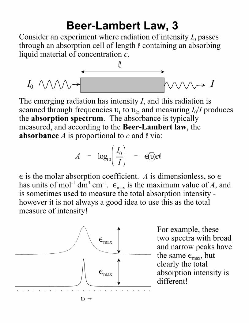
Beer-Lambert Law, 3Consider an experiment where radiation of intensity I0 passesthrough an absorption cell of length R containing an absorbingliquid material of concentration c.

L 6

,max

,max

I0 I

R

The emerging radiation has intensity I, and this radiation isscanned through frequencies L1 to L2, and measuring I0/I producesthe absorption spectrum. The absorbance is typicallymeasured, and according to the Beer-Lambert law, theabsorbance A is proportional to c and R via:

, is the molar absorption coefficient. A is dimensionless, so ,has units of mol-1 dm3 cm-1. ,max is the maximum value of A, andis sometimes used to measure the total absorption intensity -however it is not always a good idea to use this as the totalmeasure of intensity!

I

For example, thesetwo spectra with broadand narrow peaks havethe same ,max, butclearly the totalabsorption intensity isdifferent!

A ' log10

I0

I' ,(̄L)cR

The integrated area under the peak will provide a more exactmeasure of of absorption intensity. If Nn « Nm, then decay of stateNn by emission is negligible, and

If the absorption is due to an electronic transition fnm, theoscillator strength, is used to quantify the intensity and isrelated to the area under the curve by

where <nm is the average wavenumber of absorption and NA isAvogadro’s number.

The quantity fnm is dimensionless and is the ratio of the strengthof the transition to that of an electric dipole transition betweentwo states of the electron oscillating in three dimensions as asimple harmonic oscillator (max. value is typically 1).

One can also measure the transmittance, T, of a sample. If theintensity of light striking the sample is I0 and light which passesout of the sample is I, then T = I/I0, or

or, T = 10-A. Sometimes the per cent transmittance is quoted,i.e., T = 0.25, then %T = 25%.

mL̄2

L̄1

,(̄<)d(̄<) 'NAh̄ nmBnm

ln 10<

fnm '4,0mec

2ln10

NAe 2 m<̄2

<̄1

,(̄<)d<̄

A ' log10I0

I' log10

1T

' ,(̄<)cR

Absorption Intensity