Embed Size (px)
Citation preview
LIFECYCLE ASSESMENTS:METHODOLOGY & RESULTS
Environmental Working Group Meat Eaters Guide: Methodology 20112
M e a t E a t e r s G u i d e : M e t h o d o l o g y
Table of Contents
Acknowledgements . . . . . . . . . . . . . . . . . . . . . . . . . . . . . . . . . . . . . . . . . . . . . . . . . . . . . . . . . . . . . . . . . . . . . . . . . . . . . . . . .4
Introduction . . . . . . . . . . . . . . . . . . . . . . . . . . . . . . . . . . . . . . . . . . . . . . . . . . . . . . . . . . . . . . . . . . . . . . . . . . . . . . . . . . . . . . .5
A. LCA Boundaries and Functional Unit . . . . . . . . . . . . . . . . . . . . . . . . . . . . . . . . . . . . . . . . . . . . . . . . . . . . . . . . . . . . . . .5
B. Apportionment of GHGs to food versus non-food products (co-product allocation) . . . . . . . . . . . . . . . . . . . . . . . . .7
C. Modeling Agricultural Processes: Data and Emissions Factors . . . . . . . . . . . . . . . . . . . . . . . . . . . . . . . . . . . . . . . . . .7
1 . Key Inputs and Emission Outputs . . . . . . . . . . . . . . . . . . . . . . . . . . . . . . . . . . . . . . . . . . . . . . . . . . . . . . . . . . . . . . . . . . . . .7
2 . Activity Data and Criteria for Selection of Production Systems . . . . . . . . . . . . . . . . . . . . . . . . . . . . . . . . . . . . . . . . . . . . . . .9
3 . Data Sources for Calculating Emissions from Each Stage of Production . . . . . . . . . . . . . . . . . . . . . . . . . . . . . . . . . . . . . .10
4 . Model Testing, Validation, Uncertainty and Variability . . . . . . . . . . . . . . . . . . . . . . . . . . . . . . . . . . . . . . . . . . . . . . . . . . . .17
D. Modeling Emissions from Meat, Dairy and Egg Production and Consumption . . . . . . . . . . . . . . . . . . . . . . . . . . . . .21
1 . Beef Production . . . . . . . . . . . . . . . . . . . . . . . . . . . . . . . . . . . . . . . . . . . . . . . . . . . . . . . . . . . . . . . . . . . . . . . . . . . . . . . . . .24
2 . Lamb Production . . . . . . . . . . . . . . . . . . . . . . . . . . . . . . . . . . . . . . . . . . . . . . . . . . . . . . . . . . . . . . . . . . . . . . . . . . . . . . . . .27
3 . Pork Production . . . . . . . . . . . . . . . . . . . . . . . . . . . . . . . . . . . . . . . . . . . . . . . . . . . . . . . . . . . . . . . . . . . . . . . . . . . . . . . . . .29
4 . Poultry (Broiler Chicken and Turkey) . . . . . . . . . . . . . . . . . . . . . . . . . . . . . . . . . . . . . . . . . . . . . . . . . . . . . . . . . . . . . . . . . .30
5 . Dairy (Cheese) . . . . . . . . . . . . . . . . . . . . . . . . . . . . . . . . . . . . . . . . . . . . . . . . . . . . . . . . . . . . . . . . . . . . . . . . . . . . . . . . . .33
6 . Eggs . . . . . . . . . . . . . . . . . . . . . . . . . . . . . . . . . . . . . . . . . . . . . . . . . . . . . . . . . . . . . . . . . . . . . . . . . . . . . . . . . . . . . . . . . .36
7 . Farmed Salmon . . . . . . . . . . . . . . . . . . . . . . . . . . . . . . . . . . . . . . . . . . . . . . . . . . . . . . . . . . . . . . . . . . . . . . . . . . . . . . . . . .37
8 . Canned Tuna . . . . . . . . . . . . . . . . . . . . . . . . . . . . . . . . . . . . . . . . . . . . . . . . . . . . . . . . . . . . . . . . . . . . . . . . . . . . . . . . . . . .38
E. Modeling Emissions from Feedstock and Crop Production . . . . . . . . . . . . . . . . . . . . . . . . . . . . . . . . . . . . . . . . . . . . .40
1 . General Production and Modeling Details . . . . . . . . . . . . . . . . . . . . . . . . . . . . . . . . . . . . . . . . . . . . . . . . . . . . . . . . . . . . . .40
2 . Specific Modeling Details for Feedstock Production . . . . . . . . . . . . . . . . . . . . . . . . . . . . . . . . . . . . . . . . . . . . . . . . . . . . . .40
a . Corn Production . . . . . . . . . . . . . . . . . . . . . . . . . . . . . . . . . . . . . . . . . . . . . . . . . . . . . . . . . . . . . . . . . . . . . . . . . . . . . . . . . .40
b . Soybean Production . . . . . . . . . . . . . . . . . . . . . . . . . . . . . . . . . . . . . . . . . . . . . . . . . . . . . . . . . . . . . . . . . . . . . . . . . . . . . .41
c . Alfalfa Production . . . . . . . . . . . . . . . . . . . . . . . . . . . . . . . . . . . . . . . . . . . . . . . . . . . . . . . . . . . . . . . . . . . . . . . . . . . . . . . . .43
d . Lentil Production . . . . . . . . . . . . . . . . . . . . . . . . . . . . . . . . . . . . . . . . . . . . . . . . . . . . . . . . . . . . . . . . . . . . . . . . . . . . . . . . .44
3 . Sources of Emissions of Plant Protein . . . . . . . . . . . . . . . . . . . . . . . . . . . . . . . . . . . . . . . . . . . . . . . . . . . . . . . . . . . . . . . .47
Environmental Working Group Meat Eaters Guide: Methodology 2011 3
TablesTable 1 . Sources of Primary Greenhouse Gas Emissions . . . . . . . . . . . . . . . . . . . . . . . . . . . . . . . . . . . . . . . . . . . . . . . . . . . .8
Table 2 . Validation of EWG LCA GHG Emission Results of Protein-Rich Foods . . . . . . . . . . . . . . . . . . . . . . . . . . . . . . . . . .19
Table 3 . LCA Allocation Factors . . . . . . . . . . . . . . . . . . . . . . . . . . . . . . . . . . . . . . . . . . . . . . . . . . . . . . . . . . . . . . . . . . . . . . .22
Table 4 . GHG Emissions from Beef Production (at farmgate) . . . . . . . . . . . . . . . . . . . . . . . . . . . . . . . . . . . . . . . . . . . . . . . . .25
Table 5 . GHG Emissions from Beef Consumption (post-farmgate) . . . . . . . . . . . . . . . . . . . . . . . . . . . . . . . . . . . . . . . . . . . . .25
Table 6 . GHG Emissions from Lamb Production (at farmgate) . . . . . . . . . . . . . . . . . . . . . . . . . . . . . . . . . . . . . . . . . . . . . . . .28
Table 7 . GHG Emissions from Lamb Consumption (post-farmgate) . . . . . . . . . . . . . . . . . . . . . . . . . . . . . . . . . . . . . . . . . . . .28
Table 8 . GHG Emissions from Pork Production (at farmgate) . . . . . . . . . . . . . . . . . . . . . . . . . . . . . . . . . . . . . . . . . . . . . . . . .29
Table 9 . GHG Emissions from Pork Consumption (post-farmgate) . . . . . . . . . . . . . . . . . . . . . . . . . . . . . . . . . . . . . . . . . . . . .30
Table 10 . GHG Emissions from Broiler Chicken Production (at farmgate) . . . . . . . . . . . . . . . . . . . . . . . . . . . . . . . . . . . . . . .31
Table 11 . GHG Emissions from Broiler Chicken Consumption (post-farmgate) . . . . . . . . . . . . . . . . . . . . . . . . . . . . . . . . . . .31
Table 12 . GHG Emissions from Turkey Production (at farmgate) . . . . . . . . . . . . . . . . . . . . . . . . . . . . . . . . . . . . . . . . . . . . . .31
Table 13 . GHG Emissions from Turkey Consumption (post-farmgate) . . . . . . . . . . . . . . . . . . . . . . . . . . . . . . . . . . . . . . . . . .31
Table 14 . GHG Emissions from Milk Production (at farmgate) . . . . . . . . . . . . . . . . . . . . . . . . . . . . . . . . . . . . . . . . . . . . . . . .34
Table 15 . Greenhouse Gas Emission from Milk (2 percent) Consumption (post-farmgate) . . . . . . . . . . . . . . . . . . . . . . . . . .34
Table 16 . GHG Emissions from Domestic Cheese Production (at farmgate) . . . . . . . . . . . . . . . . . . . . . . . . . . . . . . . . . . . . .34
Table 17 . Greenhouse Gas Emission from Domestic Cheese Consumption (post-farmgate) . . . . . . . . . . . . . . . . . . . . . . . .34
Table 18 . GHG Emissions from Imported Cheese Production (at farmgate) . . . . . . . . . . . . . . . . . . . . . . . . . . . . . . . . . . . . .34
Table 19 . Greenhouse Gas Emission from Yogurt Consumption (post-farmgate) . . . . . . . . . . . . . . . . . . . . . . . . . . . . . . . . .35
Table 20 . GHG Emissions from Yogurt Production . . . . . . . . . . . . . . . . . . . . . . . . . . . . . . . . . . . . . . . . . . . . . . . . . . . . . . . . .35
Table 21 . GHG Emissions from Egg Production (at farmgate) . . . . . . . . . . . . . . . . . . . . . . . . . . . . . . . . . . . . . . . . . . . . . . . .36
Table 22 . GHG Emissions from Egg Consumption (post-farmgate) . . . . . . . . . . . . . . . . . . . . . . . . . . . . . . . . . . . . . . . . . . . .36
Table 23 . GHG Emissions from Imported Farmed Salmon Production (at farmgate) . . . . . . . . . . . . . . . . . . . . . . . . . . . . . . .37
Table 24 . GHG Emissions from Imported Farmed Salmon Consumption (post-farmgate) . . . . . . . . . . . . . . . . . . . . . . . . . . .38
Table 25 . GHG Emissions from Canned Tuna Production (at farmgate) . . . . . . . . . . . . . . . . . . . . . . . . . . . . . . . . . . . . . . . .39
Table 26 . GHG Emissions from Tuna Consumption (post-farmgate) . . . . . . . . . . . . . . . . . . . . . . . . . . . . . . . . . . . . . . . . . . .39
Table 27 . Iowa Corn Production System Inputs . . . . . . . . . . . . . . . . . . . . . . . . . . . . . . . . . . . . . . . . . . . . . . . . . . . . . . . . . . .41
Table 28 . Soybean Agriculture System Inputs, Major States, 2002 . . . . . . . . . . . . . . . . . . . . . . . . . . . . . . . . . . . . . . . . . . . .42
Table 29 . Production System and Primary Input Data for Feedstock & Plant Protein Products . . . . . . . . . . . . . . . . . . . . . . .45
Environmental Working Group Meat Eaters Guide: Methodology 20114
M e a t E a t e r s G u i d e : M e t h o d o l o g y
FiguresFigure 1 . Summary of Results: Total GHG Emissions from Common Proteins . . . . . . . . . . . . . . . . . . . . . . . . . . . . . . . . . . .23
Figure 2 . Sources of Production Emissions: A Nebraska System . . . . . . . . . . . . . . . . . . . . . . . . . . . . . . . . . . . . . . . . . . . . . .26
Figure 3 . Beef: Production Dominates Greenhouse Gas Emissions . . . . . . . . . . . . . . . . . . . . . . . . . . . . . . . . . . . . . . . . . . . .27
Figure 4 . Sources of GHG Emissions from British Columbia Poultry Farm . . . . . . . . . . . . . . . . . . . . . . . . . . . . . . . . . . . . . . .32
Figure 5 . Figure 5 . Chicken: Production and Post-Farmgate Emissions are Roughly Equal . . . . . . . . . . . . . . . . . . . . . . . . .32
Figure 6 . Sources of GHG Emissions for Cheese . . . . . . . . . . . . . . . . . . . . . . . . . . . . . . . . . . . . . . . . . . . . . . . . . . . . . . . . . .35
Figure 7 . Eggs: Sources of Greenhouse Gas Emissions . . . . . . . . . . . . . . . . . . . . . . . . . . . . . . . . . . . . . . . . . . . . . . . . . . . .37
Figure 8 . Tuna: Sources of Greenhouse Gas Emissions . . . . . . . . . . . . . . . . . . . . . . . . . . . . . . . . . . . . . . . . . . . . . . . . . . . .39
Figure 9 . Emission Sources of Corn Production in Iowa . . . . . . . . . . . . . . . . . . . . . . . . . . . . . . . . . . . . . . . . . . . . . . . . . . . . .41
Figure 10 . Emissions Sources of Soybean Production . . . . . . . . . . . . . . . . . . . . . . . . . . . . . . . . . . . . . . . . . . . . . . . . . . . . . .42
Figure 11 . Emissions Sources of Alfalfa Production . . . . . . . . . . . . . . . . . . . . . . . . . . . . . . . . . . . . . . . . . . . . . . . . . . . . . . . .43
Figure 12 . Sources of Lentil Production Emissions . . . . . . . . . . . . . . . . . . . . . . . . . . . . . . . . . . . . . . . . . . . . . . . . . . . . . . . . .44
AnnexesAnnex A . Activity Data Sources . . . . . . . . . . . . . . . . . . . . . . . . . . . . . . . . . . . . . . . . . . . . . . . . . . . . . . . . . . . . . . . . . . . . . . .55
Annex B . Assumptions for Cooking times and Methods . . . . . . . . . . . . . . . . . . . . . . . . . . . . . . . . . . . . . . . . . . . . . . . . . . . . .59
Annex C . Approximate Ratios of Fresh vs . Frozen Meat . . . . . . . . . . . . . . . . . . . . . . . . . . . . . . . . . . . . . . . . . . . . . . . . . . . .60
Acknowledgements EWG thanks Kumar Venkat, president of CleanMetrics, for carrying out the lifecycle data analysis and for working with EWG to define and redefine parameters, assumptions, data sources and other infor-mation underlying the analysis. We also thank him for providing important background information for this methodology as well as several thorough reviews of the document.
We also give great thanks and appreciation to Kimi Shell, our exceptional intern, for organizing much of the data and creating the numerous tables, charts, and graphs that appear throughout the docu-ment. Thanks also to Michele Reilly for her research assistance on the project.
We would also like to thank our three outside reviewers – Anna Lappe, Small Planet Institute; Dr. Roni Neff, Center for A Livable Future, Johns Hopkins University; and Dr. Whendee Silver, UC/ Berkeley – for their useful and thorough review of the first draft of this methodology.
The author would also like to thank her colleagues, Craig Cox, Renee Sharp, Lisa Frack, Sean Gray and Jane Houlihan for their edits and many contributions to the project. And finally, many thanks to the primary editor of this report, Nils Bruzelius, who has made a very long and technical document much more readable.
Environmental Working Group Meat Eaters Guide: Methodology 2011 5
By: Kari Hamerschlag, EWG Senior Analyst Kumar Venkat, President & Chief Technologist, CleanMetrics Corp.
Introduction Environmental Working Group (EWG) partnered with CleanMetrics Corp., a Portland, Ore.-based en-vironmental analysis and consulting firm, to carry out “cradle to grave” life cycle assessments (LCAs) of greenhouse gas (GHG) emissions for selected protein-rich foods, from production of animal feed to the food waste thrown in the trash.
The LCAs calculate GHG emissions from each major process, from the production and application of fertilizers, pesticides and other materials used to grow crops through to the processing, transportation and disposal of unused food at the retail, institutional and household level.1 The LCA also accounts for waste from the portion of the animal carcass that is not available for consumption.
This document provides a detailed report on the methodology, assumptions and results of the lifecycle assessments of 20 plant and animal foods commonly consumed in the United States. Due to lack of data, the analysis focused on typical, conventional food production systems rather than organic production systems or those based on best management agricultural practices that might result in lower emissions. While our LCAs focus exclusively on GHG emissions, climate impact is just one of many critical environmental and health factors to consider in evaluating protein choices. The Meat Eater’s Guide to Climate Change and Health provides a broad overview of the health and environmental concerns linked to animal production.
Section 1 addresses the boundaries (key elements included and excluded) of the LCA, the main production inputs and emission outputs, sources of data and the assumptions related to each of the main stages of production and consumption. We also provide a detailed explanation of the validation process, including a chart comparing our findings to other comparable and mostly peer-reviewed or government-sponsored LCA studies of that product. We describe many of the underlying uncertainties and variability associated with estimating GHG emissions from food production and provide concrete examples of how emissions can be reduced by better management practices. Section 2 describes the essential production, consumption and modeling details and emissions of each production system as well as the results of the GHG calculations for each based on the available input data.
A. LCA Boundaries and Functional UnitThe functional unit used to calculate GHG emissions2 is 1 kilogram of consumed, edible product. This differs considerably from the current set of published LCAs, which typically calculate only the GHGs associated with the production of one unit of edible meat or live carcass. Our model goes further to consider the GHG’s associated with material and energy expended or produced at each major stage
Environmental Working Group Meat Eaters Guide: Methodology 20116
M e a t E a t e r s G u i d e : M e t h o d o l o g y
of food production and consumption (cradle to grave), as well as the GHGs associated with the pro-duction of the amount of a given product that is necessary – given the sizable waste factor – to yield 1 kg of consumed, edible food.3
The analysis considered the following GHGs and calculated their carbon dioxide equivalents based on each one’s global warming potential (GWP) – the warming effect relative to carbon dioxide over a 100-year time frame:4
• Carbon dioxide (CO2) (GWP of 1)• Nitrous oxide (N20) (GWP of 298)• Methane (CH4) (GWP of 25)• Hydrofluorocarbons (specifically the refrigerant HFC-134a, with a GWP of 1,430).
LCAs included GHG emissions associated with the following processes5:
• Production and transport of “inputs,” the materials used to grow crops or feed animals (fertil-izers, pesticides and seed for crop production; feeds for animal production)
• On-farm generation of GHG emissions (e.g., the enteric fermentation digestive process of cows, sheep and other ruminants; manure management; soil emissions from fertilizer applica-tion; etc.)
• On-farm energy use (fuel and electricity, including energy used for irrigation)• Transportation of animals and harvested crops • Processing (slaughter, packaging and freezing)• Refrigeration (retail and transportation)• Cooking• Retail and consumer waste (waste before and after cooking, including served but uneaten
food that is thrown away)Due to lack of data, the LCAs did not consider the following processes related to food production:
• Consumer transport to and from retail outlets • Home storage of food products• Production of capital goods and infrastructure (typically excluded from most LCAs and is cur-
rently excluded from standards such as PAS 2050)• Energy required for water use in growing livestock feed (irrigation is included for alfalfa but not
for corn and soybeans)
Assessment methods used for this analysis are consistent with the globally recognized International Standards Organization (ISO) 14040 series and the British Publicly Available Specification 2050 (PAS 2050), a leading standard for life-cycle GHG emissions assessment developed at the request of the
Environmental Working Group Meat Eaters Guide: Methodology 2011 7
UK government by the UK’s national standards body, the British Standards Institution (BSI Group).
B. Apportionment of GHGs to food versus non-food products (co-product allocation)Some foods considered in this analysis are derived from animals or crops also used to make non-food products. For example, animals are used to produce meat, leather, and cosmetic ingredients, among other items. GHG emissions presented here consider only the fraction of emissions associ-ated with food production.
CleanMetrics accomplishes this allocation by apportioning GHGs from animal or crop production to food and non-food products based on – in order of preference – the relative economic value (weight-ed by mass) or a relative biophysical factor such as mass, energy or nutrition content associated with each type of finished product. This is called “co-product allocation.”
In practice, mass-weighted economic value has proved to be the most reliable basis for allocation, particularly when final products are highly dissimilar or in cases where one or most of the final prod-ucts are materials or energy other than food.6 CleanMetrics used this method for each of the food items considered in this analysis. See Table 3 for the specific allocation factors used in the calcula-tions.
Recycled materials are both produced from and used in animal- and crop-based food production. These GHG calculations model the emissions from recycling facilities and recycled materials used to grow, process, package or transport the food (e.g., recycled food packaging) using the “recycled content” method.7 For any particular food, GHG estimates include emissions from delivering waste material to a recycling facility.
C. Modeling Agricultural Processes: Data and Emissions Factors1. Key Inputs and Emission OutputsCleanMetrics modeled the GHG emissions of a number of typical, conventional (as opposed to or-ganic and/or best management) production methods for each of the foods in the Meat Eaters Guide based on a detailed inventory of inputs and outputs and associated emissions. The table below gives a sense of some, but not all, of the sources of GHG emissions considered in the LCAs.
Environmental Working Group Meat Eaters Guide: Methodology 20118
M e a t E a t e r s G u i d e : M e t h o d o l o g y
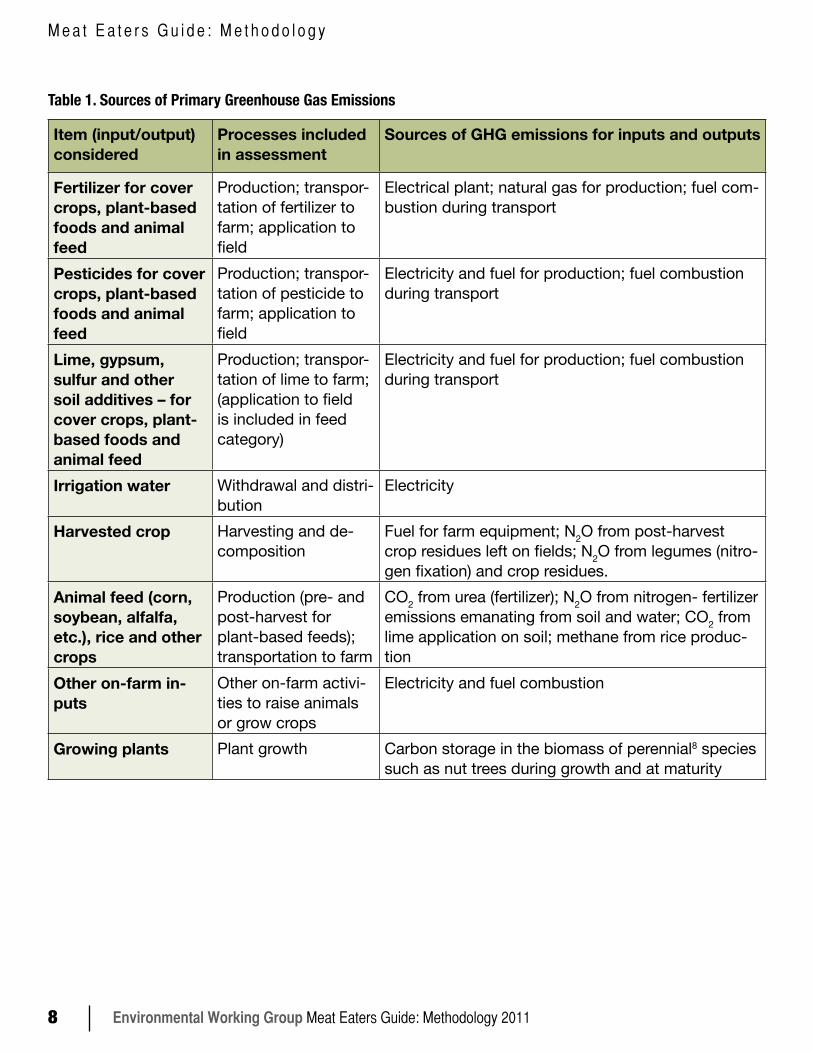
Table 1. Sources of Primary Greenhouse Gas Emissions
Item (input/output) considered
Processes included in assessment
Sources of GHG emissions for inputs and outputs
Fertilizer for cover crops, plant-based foods and animal feed
Production; transpor-tation of fertilizer to farm; application to field
Electrical plant; natural gas for production; fuel com-bustion during transport
Pesticides for cover crops, plant-based foods and animal feed
Production; transpor-tation of pesticide to farm; application to field
Electricity and fuel for production; fuel combustion during transport
Lime, gypsum, sulfur and other soil additives – for cover crops, plant-based foods and animal feed
Production; transpor-tation of lime to farm; (application to field is included in feed category)
Electricity and fuel for production; fuel combustion during transport
Irrigation water Withdrawal and distri-bution
Electricity
Harvested crop Harvesting and de-composition
Fuel for farm equipment; N2O from post-harvest crop residues left on fields; N2O from legumes (nitro-gen fixation) and crop residues.
Animal feed (corn, soybean, alfalfa, etc.), rice and other crops
Production (pre- and post-harvest for plant-based feeds); transportation to farm
CO2 from urea (fertilizer); N2O from nitrogen- fertilizer emissions emanating from soil and water; CO2 from lime application on soil; methane from rice produc-tion
Other on-farm in-puts
Other on-farm activi-ties to raise animals or grow crops
Electricity and fuel combustion
Growing plants Plant growth Carbon storage in the biomass of perennial8 species such as nut trees during growth and at maturity
Environmental Working Group Meat Eaters Guide: Methodology 2011 9
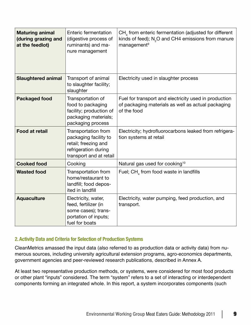
Maturing animal (during grazing and at the feedlot)
Enteric fermentation (digestive process of ruminants) and ma-nure management
CH4 from enteric fermentation (adjusted for different kinds of feed); N2O and CH4 emissions from manure management9
Slaughtered animal Transport of animal to slaughter facility; slaughter
Electricity used in slaughter process
Packaged food Transportation of food to packaging facility; production of packaging materials; packaging process
Fuel for transport and electricity used in production of packaging materials as well as actual packaging of the food
Food at retail Transportation from packaging facility to retail; freezing and refrigeration during transport and at retail
Electricity; hydrofluorocarbons leaked from refrigera-tion systems at retail
Cooked food Cooking Natural gas used for cooking10
Wasted food Transportation from home/restaurant to landfill; food depos-ited in landfill
Fuel; CH4 from food waste in landfills
Aquaculture Electricity, water, feed, fertilizer (in some cases); trans-portation of inputs; fuel for boats
Electricity, water pumping, feed production, and transport.
2. Activity Data and Criteria for Selection of Production SystemsCleanMetrics amassed the input data (also referred to as production data or activity data) from nu-merous sources, including university agricultural extension programs, agro-economics departments, government agencies and peer-reviewed research publications, described in Annex A.
At least two representative production methods, or systems, were considered for most food products or other plant “inputs” considered. The term “system” refers to a set of interacting or interdependent components forming an integrated whole. In this report, a system incorporates components (such
Environmental Working Group Meat Eaters Guide: Methodology 201110
M e a t E a t e r s G u i d e : M e t h o d o l o g y
as crops, animals, soil, etc.) within a bounded geographical area and specified time frame that takes external inputs (such as fertilizers, water, energy, etc.) and produces useful outputs (such as grains, vegetables, meat, etc.) using specific production methods. Due to limited available data, only one pro-duction method was considered for a few items, including chicken, peanut butter, lentils and orchard grass.
We selected specific conventional production systems to model based primarily on a) the availability of input data, and b) how representative it is of the industry as a whole.
We made a concerted effort to find publicly available production data from leading production regions for major meat categories. These public data sources are typically university agricultural extension programs, university agro-economics departments and state- or province-level departments of agri-culture. These sources often provide data in the form of cost and return studies or budgets that in-clude all the specific inputs consumed by a typical production system and outputs generated by the system in a specified region. We judged the quality of the data based on a number of criteria, includ-ing completeness and consistency with other data sources. We rejected some data sources that did not meet these standards (in some cases, after running a trial analysis to further evaluate the data quality).
Data was not always available for states that produce the most of some types of meat. Generally, however, we were able to find good production data from one of the top three production states for major categories such as beef and pork, as well as for dairy and eggs. We supplemented these pri-mary sources with data from other regions. The two poultry meats, chicken and turkey, are the excep-tion to this. The broiler chicken production data is from a large-scale confined feeding operation in British Columbia, Canada11 and the turkey calculations are based on data from Pennsylvania.
The data models in this analysis were based on typical production systems, rather than best-man-agement agricultural practices that might result in lower emissions. Because of differences in inputs, management practices and consumption patterns, there is some variability in the exact GHG emis-sion results for a given product. In Section 4c, we discuss how emissions might change with better management practices.
3. Data Sources for Calculating Emissions from Each Stage of ProductionUsing basic emission factors, equations and calculations from the Intergovernmental Panel on Cli-mate Change (IPCC), the U.S. Environmental Protection Agency (EPA) and other recognized sources described below, CleanMetrics analyzed each aspect of the input data to calculate the GHGs associ-ated with each activity along the supply chain.
The analysis used emission factors and calculations for the extraction and combustion of primary fuels – as well as non-energy-related factors for GHG emissions inherent in industrial, agricultural, transport and other processes – generated primarily from the following two sources:
Environmental Working Group Meat Eaters Guide: Methodology 2011 11
a)US Life-Cycle Inventory (LCI) Database (NREL 2010);
b)IPCC Guidelines for National Greenhouse Gas Inventories (IPCC 2010).
Additional sources and assumptions behind our emission estimates follow, detailing the assumptions behind the estimates of greenhouse gas emissions generated during the pre-farm gate phase.
a. ElectricitySeveral stages of food production consume electric power. Primary energy use and GHG emissions per unit of electricity supplied through the grid were calculated using activity data consisting of fuel and power plant mixes for various grid regions (both US and international), as well as transmission losses and other details, drawn from:
a) EPA eGRID Emissions Database
b) IEA Energy Statistics (Electricity/Heat by Country/Region).
For the processing stage, the analysis used average US electricity emissions, except in a few cases (such as chicken and turkey) where the processing is likely to occur in the same state/province as the production systems. All US electricity production data are derived from EPA’s eGRID database; inter-national electricity production data are from the International Energy Agency’s country-level statistics.
b. TransportPractically all production phases require the use of transportation of inputs and outputs. Primary energy use and GHG emissions per metric ton-kilometer of freight for all transport modes (road, rail, ocean and air) were calculated using activity data from: a) Greenhouse Gas Protocol, and b) DOE Transportation Energy Data Book.
Transport assumptions• The analysis assumes domestic sourcing of all manufactured inputs for the farm (such as feed
and fertilizer). 12 • The model assumes that farm inputs are transported a distance of 1,600 km by semi-trailer
trucks to a local distribution center, and an additional 200 km by single-unit trucks to the farm.13 14
• Locally available organic materials – such as compost, manure and hay – are assumed to be transported 300 km to the farm by single-unit trucks.
• All animal transport to meat processing assumes a distance of 300 km.15
• All waste (retail and consumer) is assumed to be transported 100 km.• Packaging materials are assumed to be transported 1,600 km to processing facilities by semi-
Environmental Working Group Meat Eaters Guide: Methodology 201112
M e a t E a t e r s G u i d e : M e t h o d o l o g y
trailer truck.• All food items are assumed to be produced and transported domestically, with the exception
of lamb and salmon, which are assumed to be imported and transported via ship a distance equal to the average distance of the top two producing countries. Lamb production data is domestic; our calculations assume that 50% is imported by ship from New Zealand and Aus-tralia.
• All food products are assumed to travel 2,253 km (1,500 miles) and by semi-trailer truck 161 km (100 miles) by single-unit truck to final retail establishment. 16
• For imported products (lamb, salmon, imported cheese), we estimate emissions for each item using the average distance (in nautical miles) from the top two exporting countries.
• All transport modes are assumed to have 100 percent utilization (full use of the truck) and 100 percent backhaul (use of the return trip for hauling other freight).
Clearly, the actual distance traveled by different inputs will vary by region and production system. In some cases, animals are trucked much farther than 300 km from where they are born to where they are raised in confinement. The distance that food travels to its final destination will also vary. For the purposes of this analysis, we selected a set of consistent assumptions based on general averages. In order to provide a sense of the differential GHG impact of eating locally or regionally, our model calcu-lated GHGs of food that was transported either 2,253 km or 161 km (100 miles). Surprisingly, the ac-tual GHG differential between 2,253 km and 161 km is quite small. In the case of beef, eating a kilo-gram of beef that travelled 161 versus 2,253 km only changes the GHG footprint by 0.28 kg CO2e per kg of beef consumed – less than 1 percent of beef’s total emissions. The difference is much greater in vegetables, where the overall footprint is much smaller. Buying locally can reduce the overall footprint by as much as 20 percent for broccoli and 25 percent for tomatoes; local purchasing reduces meat’s carbon footprint by just 1-3 percent. We also considered the GHGs associated with shipping products such as cheese and lamb (about 50 percent of lamb is imported). Shipping adds 0.18 kg CO2e per kg beef, but just 0.06 kg CO2e per kg of cheese.
c. Fertilizer and Pesticide ProductionFertilizer production is an energy-intensive process that relies primarily on natural gas. Pesticide production is also energy intensive, relying primarily on the use of crude petroleum oils and/or natural gas. CO2 is generated from the energy used in production and in treating the resulting wastewater.
CleanMetrics based emission factors for fertilizer production on International Fertilizer Association (IFA) publications.17 Pesticide data were derived from the Encyclopedia of Pest Management.Water/wastewater treatment data are from American Council for an Energy Efficient Economy (ACEEE) and IPCC. Emissions associated with transportation of fertilizers and pesticides to the agricultural sites are based on an assumption of 1,600 km by semi-trailer truck and 200 km by single-unit truck.18
Environmental Working Group Meat Eaters Guide: Methodology 2011 13
d. Feed ProductionThe four main feed stocks modeled in the LCAs are domestic corn, soybeans, orchard grass and alfalfa.19 Feed production requires significant fuel, water and energy to produce and apply pesticides and fertilizer and to grow and feed crops. CleanMetrics estimated fertilizer, pesticides, fuel, irrigation and electricity quantities used in feed production based on input data cited in Table 27 and 28. Sec-tion E2 provides further details about the sources of emissions from the production of corn, soybean, and alfalfa, the three primary animal feed stocks.
CleanMetrics used IPCC Tier 1 methods in modeling emissions from agricultural soils from fertilizer application for growing feed (including grazing, where appropriate). These emissions include direct and indirect nitrous oxide emissions generated from synthetic and organic nitrogen fertilizers and crop residues, as well CO2 from the application of lime and urea. The model also includes indirect nitrous oxide emissions from aquaculture systems as a function of nitrogen added or released into the water.
e. Enteric Fermentation and Manure ManagementRuminant animals such as sheep and cows emit methane from enteric fermentation, a digestive pro-cess in which microorganisms break down carbohydrates into simple molecules for better absorption. All animals generate methane and nitrous oxide from manure deposits.
CleanMetrics used IPCC tier 2 methods to model emissions from livestock production. Calculations for methane from enteric fermentation are based on the kind of feedstuffs ingested by livestock spe-cies and the quality of the ingredients in the feed mix. For example, feedstuffs with higher fiber con-tent, such as grass and hay, generate higher emissions than a higher quality, grain-based diet. 20
Methane emission estimates from manure management are based on the type of manure manage-ment system (pasture, solid storage, liquid), the average temperature of the geographic location, and the amount of volatile solids excreted (in turn based on feed energy content and digestibility). Direct and indirect nitrous oxide emissions from manure are calculated based on nitrogen balance (in turn based on crude protein content in the diet) and the quantities of nitrogen excreted. Emission factors vary depending on the actual manure management system (such as pasture, dry lot, solid storage, liquid/slurry, poultry manure with/without litter, etc.).21
f. Soil Carbon Emissions and SequestrationNet carbon can be emitted from or sequestered in soil depending on the kinds of agricultural practices employed on the land and whether the system is in transition or steady state. While certain types of management practices, such as tillage and intensive grazing, are known to generate a loss of carbon, other practices such as rotational grazing and organic fertilization are known to build up carbon in the soil (see Best Management Practices section below).
Rates of soil carbon sequestration and emissions from soils differ under different land management
Environmental Working Group Meat Eaters Guide: Methodology 201114
M e a t E a t e r s G u i d e : M e t h o d o l o g y
regimes, but these differences remain poorly understood.22 As a result, this analysis does not con-sider the carbon sequestration benefits or the carbon losses that could be occurring during a transi-tion phase as a result of changes in soil management practices. For the results presented here, we assume that direct land use and management practices have been unchanged for a sufficiently long period and that soil carbon is at equilibrium. According to the IPCC, soil carbon content is considered to approach over time “a spatially-averaged, stable value specific to the soil, climate, land-use and management practices.” 23 Under this assumption, unless management practices have changed re-cently (for example, within the IPCC default transition period of 20 years between equilibrium values) on a given cropland, the soil carbon content is considered to be unchanged (or in “steady state”).
Although the IPCC states that this “assumption…is widely accepted,” 24 it should be pointed out that assumptions about steady state remain the subject of considerable scientific debate. Several recent studies have reported ongoing carbon losses on intensively managed soil for extended periods25. While we recognize that this assumption could be a limitation in the analysis, this is a standard as-sumption in most current published LCAs of food products. 26
g. Methane Emissions from Rice ProductionMethane is produced from anaerobic decomposition in flooded rice fields. Emission factors are based on IPCC tier 1 parameters.
h. Processing Due to lack of available domestic data, meat-processing calculations for beef, lamb and pork are based on average data from New Zealand27: 0.019 cubic meters of natural gas and 0.286 kwh of elec-tricity per kg of carcass weight. This is applied to US conditions using average US national or regional electricity emissions data.
i. PackagingFood packaging uses materials such as plastics, glass, metal, paper and cardboard. GHG emis-sions for many basic manufacturing processes and materials used in food packaging were calculated through an analysis of the US Life-Cycle Inventory Database. Additional data sources for materials include the Inventory of Carbon and Energy, Eco-Profiles of the European Plastics Industry, peer-reviewed research publications, LCA/LCI studies in the public domain and industry sources. Case-ready meat/seafood packaging configuration and size were obtained from a meat and seafood com-mercial package manufacturer (http://www.sealedair.com/special/nmcs_summary.pdf and http://www.sealedair.com/products/food/caseready/default.html). Other package configurations and sizes were estimated based on actual measurements of packages.
j. Refrigeration and FreezingInitial freezing of any food commodity is an energy-intensive operation, often exceeding the energy
Environmental Working Group Meat Eaters Guide: Methodology 2011 15
required to maintain the product at low temperatures during transport and storage.
• GHG emission calculations for refrigerated warehouse storage, retail and transportation are based on activity data for primary energy use from EPA Energy Star and fluorocarbon emission data from IPCC.
• GHG emission calculations for initial freezing are based on energy estimates from EnergyStar (http://www.energystar.gov/ia/business/industry/Food-Guide.pdf).
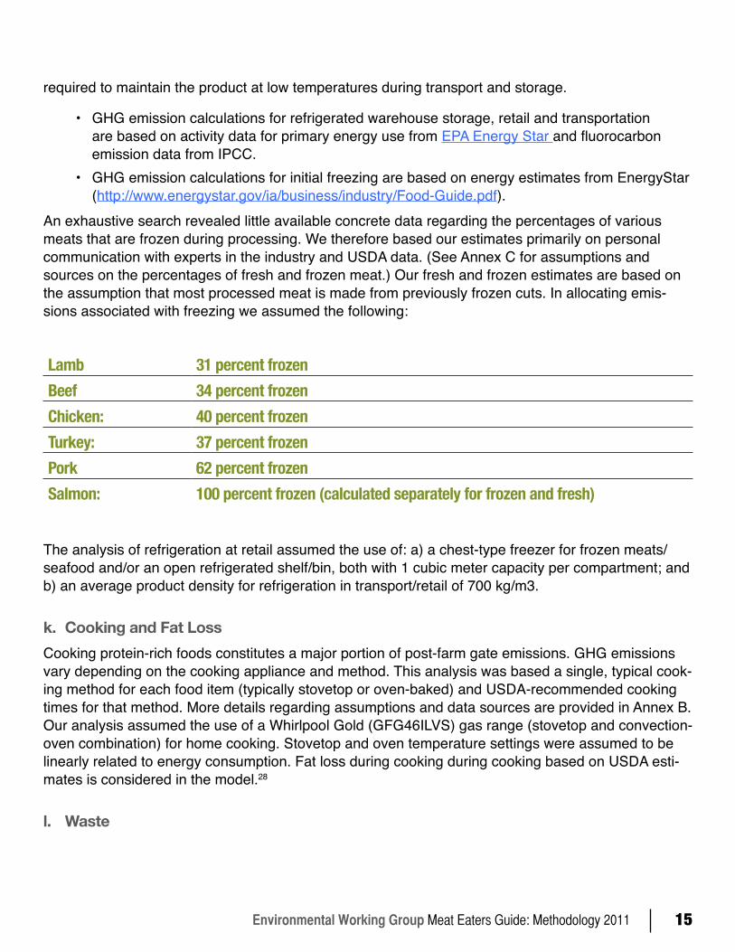
An exhaustive search revealed little available concrete data regarding the percentages of various meats that are frozen during processing. We therefore based our estimates primarily on personal communication with experts in the industry and USDA data. (See Annex C for assumptions and sources on the percentages of fresh and frozen meat.) Our fresh and frozen estimates are based on the assumption that most processed meat is made from previously frozen cuts. In allocating emis-sions associated with freezing we assumed the following:
Lamb 31 percent frozenBeef 34 percent frozenChicken: 40 percent frozenTurkey: 37 percent frozen Pork 62 percent frozenSalmon: 100 percent frozen (calculated separately for frozen and fresh)
The analysis of refrigeration at retail assumed the use of: a) a chest-type freezer for frozen meats/seafood and/or an open refrigerated shelf/bin, both with 1 cubic meter capacity per compartment; and b) an average product density for refrigeration in transport/retail of 700 kg/m3.
k. Cooking and Fat LossCooking protein-rich foods constitutes a major portion of post-farm gate emissions. GHG emissions vary depending on the cooking appliance and method. This analysis was based a single, typical cook-ing method for each food item (typically stovetop or oven-baked) and USDA-recommended cooking times for that method. More details regarding assumptions and data sources are provided in Annex B. Our analysis assumed the use of a Whirlpool Gold (GFG46ILVS) gas range (stovetop and convection-oven combination) for home cooking. Stovetop and oven temperature settings were assumed to be linearly related to energy consumption. Fat loss during cooking during cooking based on USDA esti-mates is considered in the model.28
l. Waste
Environmental Working Group Meat Eaters Guide: Methodology 201116
M e a t E a t e r s G u i d e : M e t h o d o l o g y
An astounding amount of meat – on average about 20 percent – is wasted at the retail, institutional and consumer level. The GHGs associated with producing and discarding wasted food is calculated using a recently commissioned USDA study (Muth, et al 2011) of consumer-level food loss estimates at the retail and household levels, and other literature sources for estimates of fat loss (included in USDA data) and moisture loss (not included in USDA data) during cooking.
USDA states that these data are more accurate than previously published USDA data, but they are still likely underestimating actual waste.29 At least two other major studies have generated higher retail and consumer waste estimates.30 Given data limitations, our model considers only the waste from the retail and consumer phases (including institutions and restaurants) for each food commodity. Our calculations do not include wasted product that remains on farmers’ fields or waste generated from processing. In the absence of solid data, our model conjectures that half of the consumer waste (ex-cluding fat and moisture losses) occurs prior to cooking and the other half occurs after cooking. The overall model also accounts for fat and moisture losses during cooking, as well as waste that occurs prior to cooking – including retail waste and non-edible share (such as egg shells or broccoli stems). For meat products, only the edible share is included in the model based on co-product allocation at the production stage.
Based on that waste percentage, we calculate the GHGs associated with the amount of a given prod-uct that is needed to produce 1 kg of consumed product. In other words, if the production is P kg, and the waste percentage is W percent, then: P = 1/(1-(W/100)).
Here is how our model works in the case of beef. Recent USDA research shows that 23.44 percent of the weight of packaged beef is never used, is wasted during cooking or discarded after a meal.31 This includes a retail loss of 4.3 percent and further losses at the consumer level. Relative to the con-sumer loss portion, available data suggests that 7 percent is fat loss that occurs during cooking and is included in the USDA waste data. An additional 18 percent of weight loss (relative to product available after other losses) occurs during cooking from moisture loss, which we assume is not included in the USDA waste data – this requires production and waste to be scaled up appropriately to deliver 1 kg of cooked product for consumption. We therefore calculate that it takes 1.59 kg of beef to produce 1 kg of consumed meat, and 0.59 kg is lost during the retail and consumption phase.32 Actual waste that is disposed through landfilling or composting amounts to 0.27 kg, the balance being the fat and mois-ture losses during cooking.
All food waste sent to landfills is modeled using the same IPCC first-order model33 and decay rate for the food category (for example, all meat is assumed to decay at the same rate, with no difference between chicken and lamb). The only difference between various food commodities is the estimated percentage of food waste. We assumed that the landfill was located in a temperate dry zone. (A temperate wet zone has slightly higher emissions). The food waste that ends up in landfills generates methane emissions from anaerobic decomposition as well as a small amount of nitrous oxide emis-sions. Our model assumes that 23.25 percent of the landfill methane is captured on average (with credit given for energy recovery) and 21 percent of the methane is flared (EPA2006), and some credit is given for carbon storage in the landfill. The analysis also calculates emissions from the transport of
Environmental Working Group Meat Eaters Guide: Methodology 2011 17
used packaging materials to waste disposal (landfill or recycling facility).
Our models also provided a calculation to measure GHGs when food is composted. On average, composting (at home or through a service) reduces overall emissions by small amounts compared to landfilling: less than 1-3 percent for all meats and just 10 percent for broccoli and tomatoes. This is a result of the model assumptions on how the landfill methane is managed.
Emissions from the disposal of packaging materials, including cardboard, Styrofoam, plastic wrap, plastic containers and glass bottles, are ignored since all cardboard used in packaging (the only packaging material that is likely to decompose in a landfill within a 100-year assessment period) is as-sumed to be recycled. The costs and benefits of recycling are allocated to other product systems that use the recycled material in some form (according the “recycled content” method34). All plastic and glass packaging materials are either landfilled or recycled. If landfilled, they do not degrade within a 100-year assessment period and therefore do not add to the product life cycle emissions.
4. Model Testing, Validation, Uncertainty and VariabilityThe LCA models for all the crop and animal production systems were put through a number of stan-dard steps for model testing and validation, most of which were done automatically by the CleanMet-rics LCA software. These included:
• Sensitivity analysis on explicit numerical assumptions where actual data were not available, such as transport distances for inputs used in crop production and transport distance from farm to meat processing.
• Mass and energy balance where appropriate.• Crosschecking of input values amongst multiple product systems producing the same or
similar commodity for consistency.• Checking of both input and output values to flag those that fall well outside normal ranges.• Weeding out a small number of production systems where the data appeared to be erroneous
or of poor quality in some way.
a. ValidationIn order to validate the general findings of our analysis, EWG gathered data results for the GHG emissions produced by 1 kg of each food product produced (prior to processing) by comparing them to several other mostly peer-reviewed or government-sponsored LCA GHG studies for those products in the US, Canada and Europe.35 EWG’s results were within a 2-50 percent range of the studies listed below, though in most cases, our results were within a 5-10 percent range of at least one other study.
Nevertheless, it is important to note that the goal of this study is not to predict with absolute certainty the exact GHG emissions associated with a portion of meat or protein alternative. Instead it is to give a general sense of the magnitude of GHGs associated with meat consumption and provide general
Environmental Working Group Meat Eaters Guide: Methodology 201118
M e a t E a t e r s G u i d e : M e t h o d o l o g y
guidance of the relative GHGs of different proteins.
Predicting GHG emissions with absolute certainty is difficult. Actual GHG emissions associated with a given product will vary depending on: 1) the extent to which best practices are implemented along the entire supply chain; and 2) differences in input data as a result of regional and/or production system differences for a for a given meat/crop production system. There are also uncertainties associated with IPCC emission factors. We discuss all these factors in some detail below.
Given the validation results, however, we are confident that our report provides good guidance on the relative carbon footprints of different kinds of meat and plant proteins as well as a good basis for com-paring overall life cycle carbon footprints of consuming these foods with other human activities.
b. Uncertainty and variability associated with input data and process assumptions Additional uncertainties arise from the variability of activity data used to model specific production systems as well as assumptions related to background processes. For example, the specific input data used for modeling beef production systems could be different in Idaho and Nebraska than in Kansas, or the length of time in the feedlot might vary. Similarly, there may be differences in inputs and transportation distances between one production system and another. In several cases, we were unable to find data from the states with the highest production for a particular kind of meat. Neverthe-less, we are confident that the systems we modeled are fairly representative and comparable in terms of inputs used and emissions generated across production systems.
Since virtually all input and output data were obtained from external sources (listed elsewhere) as single-point estimates, we have no information on uncertainty related to those estimates.
The specific GHG CO2e value that we present for each product is typically the average of two or three production systems from two or more regions that we modeled. The range for GHG emissions associ-ated with a given product, as well as the average, is presented in Section D.
Environmental Working Group Meat Eaters Guide: Methodology 2011 19
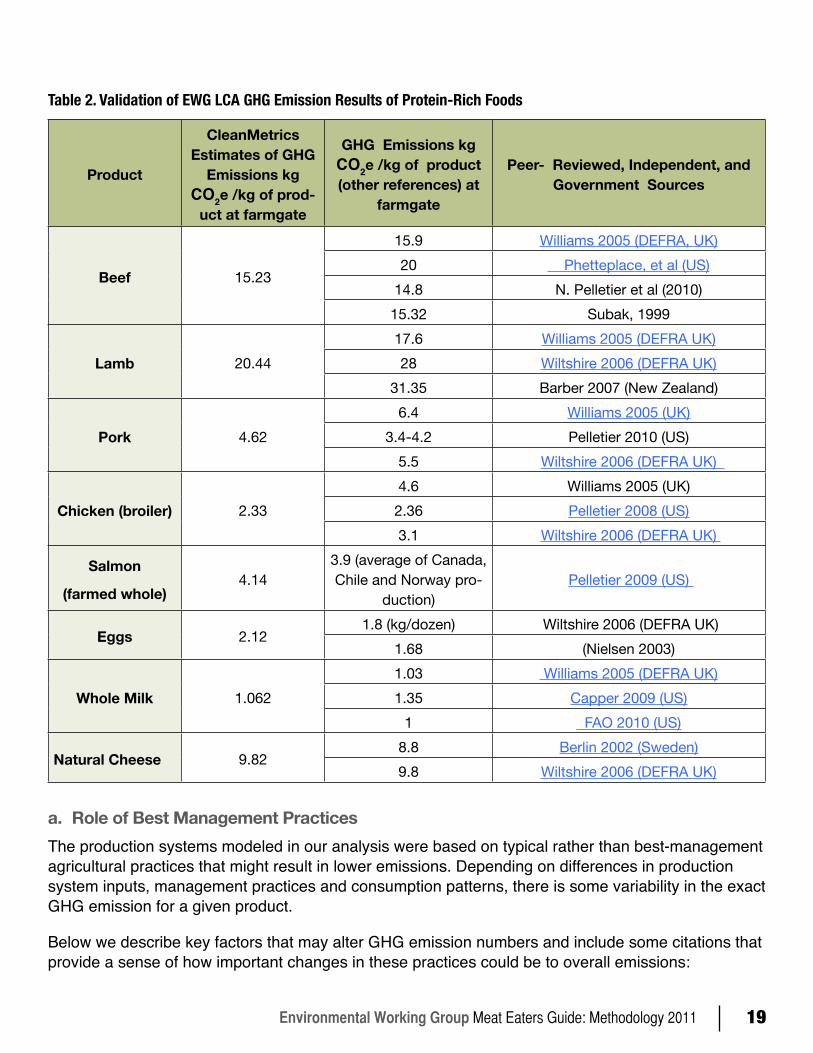
Table 2. Validation of EWG LCA GHG Emission Results of Protein-Rich Foods
Product
CleanMetrics Estimates of GHG
Emissions kg CO2e /kg of prod-
uct at farmgate
GHG Emissions kg CO2e /kg of product (other references) at
farmgate
Peer- Reviewed, Independent, and Government Sources
Beef 15.23
15.9 Williams 2005 (DEFRA, UK)20 Phetteplace, et al (US)
14.8 N. Pelletier et al (2010)15.32 Subak, 1999
Lamb 20.4417.6 Williams 2005 (DEFRA UK)28 Wiltshire 2006 (DEFRA UK)
31.35 Barber 2007 (New Zealand)
Pork 4.62 6.4 Williams 2005 (UK)
3.4-4.2 Pelletier 2010 (US)5.5 Wiltshire 2006 (DEFRA UK)
Chicken (broiler) 2.334.6 Williams 2005 (UK)2.36 Pelletier 2008 (US)3.1 Wiltshire 2006 (DEFRA UK)
Salmon
(farmed whole)4.14
3.9 (average of Canada, Chile and Norway pro-
duction)Pelletier 2009 (US)
Eggs 2.121.8 (kg/dozen) Wiltshire 2006 (DEFRA UK)
1.68 (Nielsen 2003)
Whole Milk 1.0621.03 Williams 2005 (DEFRA UK)1.35 Capper 2009 (US)
1 FAO 2010 (US)
Natural Cheese 9.828.8 Berlin 2002 (Sweden)9.8 Wiltshire 2006 (DEFRA UK)
a. Role of Best Management Practices The production systems modeled in our analysis were based on typical rather than best-management agricultural practices that might result in lower emissions. Depending on differences in production system inputs, management practices and consumption patterns, there is some variability in the exact GHG emission for a given product.
Below we describe key factors that may alter GHG emission numbers and include some citations that provide a sense of how important changes in these practices could be to overall emissions:
Environmental Working Group Meat Eaters Guide: Methodology 201120
M e a t E a t e r s G u i d e : M e t h o d o l o g y
• Overall Efficiency of the Agricultural Operation: Greater yields per input will naturally result in lower GHGs; more productive agricultural systems tend to produce the fewest GHGs per unit. This is perhaps one of the most important factors that could change the relative GHGs of a given operation. However, in some cases efficiency gains can be counteracted by unintended consequences. For example, feed production efficiency gains could be achieved by increased fertilizer use, which could in turn lead to increased nitrous oxide emissions.36
• Nutritional quality and digestibility of feed: High quality diets (based on ingredients such as corn and soy) will result in lower methane emissions from the cow’s digestive process compared to lower quality, higher-fiber diets consisting of grass and hay.37
• Manure Management Practices: Solid manure storage will have lower methane emissions than open pit or liquid manure systems; ensuring that manure is then spread on fields in an ef-ficient manner (not overusing manure and assuming no precipitation) will also reduce the N20 emissions from application of manure.38
• Grazing Practices: Intensive grazing (whereby animals are regularly moved to fresh pasture to maximize the quality and quantity of forage growth) generates fewer GHGs than the more common practice of extensive grazing.39 Other best management practices, such as the use of soil amendments, could result in steady sequestration of carbon by pastureland and would reduce the overall emissions of this stage of the process.40
• Soil Management Practices: Various best practices in soil management, such as cover cropping and composting, result in lower emissions by building soil organic carbon. At the same time, reducing fertilizer use for growing feed (especially corn) could result in decreases in energy use from fertilizer production as well as decreases in nitrous oxide emissions.41 Since feed production contributes a sizable amount to the overall carbon footprint of meat, best management practices in fertilizer application could be an important way to reduce GHG emissions.
• Freezing: Whether a product is frozen or not has an important impact on post-farmgate emis-sions but not on a product’s overall emissions. For example, consuming fresh rather than frozen beef reduces its GHG emissions by less than 3 percent.
• Cooking: The length and type of cooking has an important impact on post-farmgate emis-sions. For example, a baked potato has a much higher GHG impact than French fried potatoes, since French fries are cooked in about 5 minutes while a baked potato takes about an hour.42 However, cooking accounts for a relatively small portion of the overall footprint in the case of animal products (about 4 percent in the case of beef).
• Waste: The percentage of food that is wasted along the supply chain has a dramatic impact on the carbon footprint of food when all the inputs that went into producing that food are con-sidered. Whether a food item is composted or sent to the dump also has an impact, but not nearly as much as the actual amount of food discarded. According to our model, composting beef rather than tossing it in the garbage reduces the overall carbon footprint by .4 percent (26.93 CO2 if beef is composted instead of 27.02 if it is tossed in the landfill).
Environmental Working Group Meat Eaters Guide: Methodology 2011 21
d. Sensitivity Analysis: Each crop or animal production system may include up to 30 different inputs/outputs with specific values. Moreover, it is generally true that there are strong correlations among some inputs and outputs in any production system (i.e., a change in one might imply changes in oth-ers), but these relationships are not easily quantifiable. Due to lack of data about uncertainties and correlations, as well as the large number of input/output variables in each system, it has not been possible or useful to conduct a comprehensive numerical sensitivity analysis on input/output values for all production systems.
e. Uncertainty Associated with GHG Emissions Agricultural Production Systems and IPCC fac-tors
In general, there is significant variability and uncertainty with respect to greenhouse gas emissions from agricultural systems. This analysis relies on widely accepted IPCC emission factors for underly-ing biochemical processes (such as methane from enteric fermentation and nitrous oxide from fer-tilizer application). While these are tailored to specific agricultural systems and conditions, (dry vs. temperate climates, grass- vs. grain-feed, dry vs. liquid manure storage, etc.), they are based on av-erages and, in some cases, very few field measurements – and therefore actual emissions may vary considerably depending on particular conditions.
Nitrous oxide emissions, in particular, are inherently highly variable and hard to measure with great certainty, given different microbial, soil and weather conditions. Some have estimated that the nitrous oxide emission factor could vary by as much as 50 percent.43 Similarly the CO2 associated with lime application (a common feature in soybean production) is also known to have variability as high as 50 percent, according to the IPCC and other studies.44 Whether this variability could significantly change our GHG calculation depends on the relative contribution of corn feed (and N20) to the overall foot-print. In the case of chicken, feed (mostly corn) represents 53 percent of pre-farmgate (production emissions) and about half of those are N20 soil emissions (see section D for details). However, since feed comprises only 18 percent of total chicken emissions, reducing N20 emissions significantly would only make a small difference in the overall GHG footprint.
It should be noted that with respect to methane, estimates on feed conversion to methane and meth-ane emissions from manure tend to be less variable. Therefore, for production systems such as beef, where methane constitutes the largest emission source, there is greater certainty as to the overall carbon footprint. The uncertainty associated with GHG emissions from agriculture is the subject of an ongoing debate and the best that we can do at the moment is rely on the most reasonable estimates as developed by the IPCC.
D. Modeling Emissions from Meat Production and Consumption This section describes the essential production, consumption and modeling details and emissions of selected geographical meat production systems included in EWG Meat Eaters Guide. We provide key calculations explaining how the waste factor is integrated into the model, as well as the key assump-tions behind choices for determining the edible portion of meat.
Environmental Working Group Meat Eaters Guide: Methodology 201122
M e a t E a t e r s G u i d e : M e t h o d o l o g y
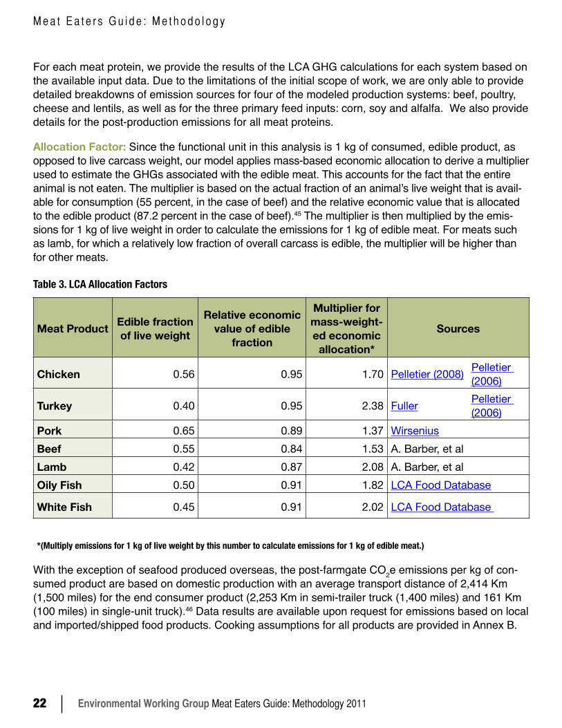
For each meat protein, we provide the results of the LCA GHG calculations for each system based on the available input data. Due to the limitations of the initial scope of work, we are only able to provide detailed breakdowns of emission sources for four of the modeled production systems: beef, poultry, cheese and lentils, as well as for the three primary feed inputs: corn, soy and alfalfa. We also provide details for the post-production emissions for all meat proteins.
Allocation Factor: Since the functional unit in this analysis is 1 kg of consumed, edible product, as opposed to live carcass weight, our model applies mass-based economic allocation to derive a multiplier used to estimate the GHGs associated with the edible meat. This accounts for the fact that the entire animal is not eaten. The multiplier is based on the actual fraction of an animal’s live weight that is avail-able for consumption (55 percent, in the case of beef) and the relative economic value that is allocated to the edible product (87.2 percent in the case of beef).45 The multiplier is then multiplied by the emis-sions for 1 kg of live weight in order to calculate the emissions for 1 kg of edible meat. For meats such as lamb, for which a relatively low fraction of overall carcass is edible, the multiplier will be higher than for other meats.
Table 3. LCA Allocation Factors
Meat Product Edible fraction of live weight
Relative economic value of edible
fraction
Multiplier for mass-weight-ed economic allocation*
Sources
Chicken 0.56 0.95 1.70 Pelletier (2008) Pelletier (2006)
Turkey 0.40 0.95 2.38 Fuller Pelletier (2006)
Pork 0.65 0.89 1.37 WirseniusBeef 0.55 0.84 1.53 A. Barber, et alLamb 0.42 0.87 2.08 A. Barber, et alOily Fish 0.50 0.91 1.82 LCA Food Database
White Fish 0.45 0.91 2.02 LCA Food Database
*(Multiply emissions for 1 kg of live weight by this number to calculate emissions for 1 kg of edible meat.)
With the exception of seafood produced overseas, the post-farmgate CO2e emissions per kg of con-sumed product are based on domestic production with an average transport distance of 2,414 Km (1,500 miles) for the end consumer product (2,253 Km in semi-trailer truck (1,400 miles) and 161 Km (100 miles) in single-unit truck).46 Data results are available upon request for emissions based on local and imported/shipped food products. Cooking assumptions for all products are provided in Annex B.
Environmental Working Group Meat Eaters Guide: Methodology 2011 23
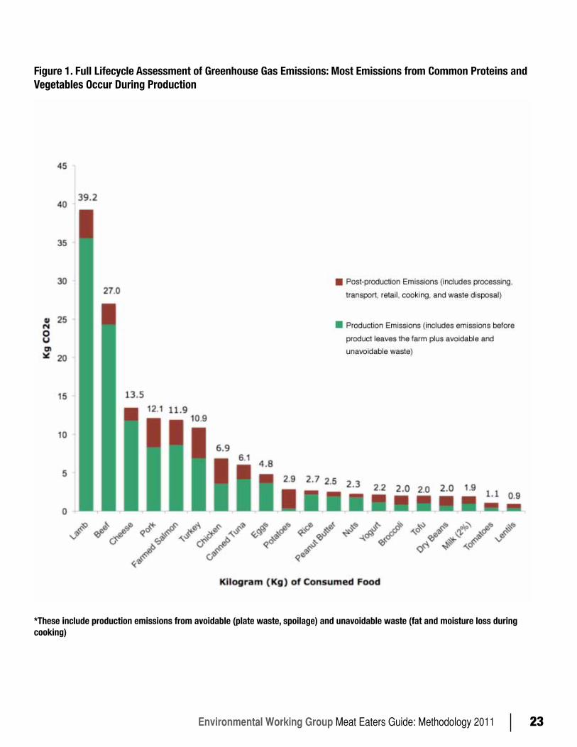
Figure 1. Full Lifecycle Assessment of Greenhouse Gas Emissions: Most Emissions from Common Proteins and Vegetables Occur During Production
*These include production emissions from avoidable (plate waste, spoilage) and unavoidable waste (fat and moisture loss during cooking)
Environmental Working Group Meat Eaters Guide: Methodology 201124
M e a t E a t e r s G u i d e : M e t h o d o l o g y
1. Beef ProductionBeef production systems are more complex than many other animal production systems. The cradle-to-farmgate life cycle assessment considered two conventional beef production systems:
• A two-stage system based in Idaho; • The more common three-stage system based on input data from Nebraska, the third leading
cattle producing state in the country.47 Our GHG estimate was based on the average GHG emissions of the Idaho and Nebraska beef pro-duction systems. Nebraska is the nation’s third largest cattle producing state. Our analysis did not consider the leading cattle-producing states due to lack of data.
The three-stage system based on Nebraska input data consists of the cow-calf, steer calf (stocker) and finishing (feedlot) phases, each with its own distinct set of inputs (fuel, electricity, feed) and out-puts (CO2, methane and nitrous oxide).
a. Key Production and Modeling DetailsCow-calf stage:
• In the Nebraska system, cows and calves are fed in a lot nearly year-round on mostly hay and some corn silage. The system we studied does not rely on grazing, although other cow-calf systems in Nebraska and elsewhere do.
• The cow-calf stage in the Idaho system includes a pasture component with hay supplements; in addition to grazing on grass, feed includes significant amounts of hay and crop residues
• The manure management for the cow-calf systems in both Idaho and Nebraska assume a pasture-like system.48
• Once the calves reach 550 lbs., they are separated from the cows and sent to a stocker (steer calf) operation.
• Other inputs include feed supplements such as salt and minerals and fuel.• Replacement cows are usually raised within the herd. Twenty percent of calves are retained
for replacement. • Herd size and operation size are not available for these beef production systems because the
data used for analysis were provided per cow-calf unit or per confined animal.Steer calf (stocker) phase:
• Steers are fed a mixed diet of hay, grain such as corn, soymeal and supplements for 180 days and fattened up to about 715 lbs. Animals are primarily fed in a barn or confined lot where their manure is collected and stored in a dry storage facility.49
• The operation uses diesel for fuel requirements.
Environmental Working Group Meat Eaters Guide: Methodology 2011 25
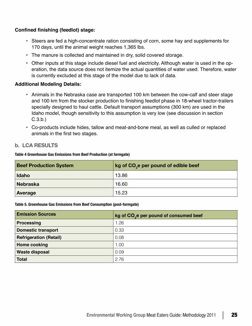
Confined finishing (feedlot) stage:
• Steers are fed a high-concentrate ration consisting of corn, some hay and supplements for 170 days, until the animal weight reaches 1,365 lbs.
• The manure is collected and maintained in dry, solid covered storage.• Other inputs at this stage include diesel fuel and electricity. Although water is used in the op-
eration, the data source does not itemize the actual quantities of water used. Therefore, water is currently excluded at this stage of the model due to lack of data.
Additional Modeling Details:
• Animals in the Nebraska case are transported 100 km between the cow-calf and steer stage and 100 km from the stocker production to finishing feedlot phase in 18-wheel tractor-trailers specially designed to haul cattle. Default transport assumptions (300 km) are used in the Idaho model, though sensitivity to this assumption is very low (see discussion in section C.3.b.)
• Co-products include hides, tallow and meat-and-bone meal, as well as culled or replaced animals in the first two stages.
b. LCA RESULTSTable 4 Greenhouse Gas Emissions from Beef Production (at farmgate)
Beef Production System kg of CO2e per pound of edible beef
Idaho 13.86
Nebraska 16.60
Average 15.23
Table 5. Greenhouse Gas Emissions from Beef Consumption (post-farmgate)
Emission Sources kg of CO2e per pound of consumed beefProcessing 1.26Domestic transport 0.33Refrigeration (Retail) 0.08Home cooking 1.00Waste disposal 0.09Total 2.76
Environmental Working Group Meat Eaters Guide: Methodology 201126
M e a t E a t e r s G u i d e : M e t h o d o l o g y
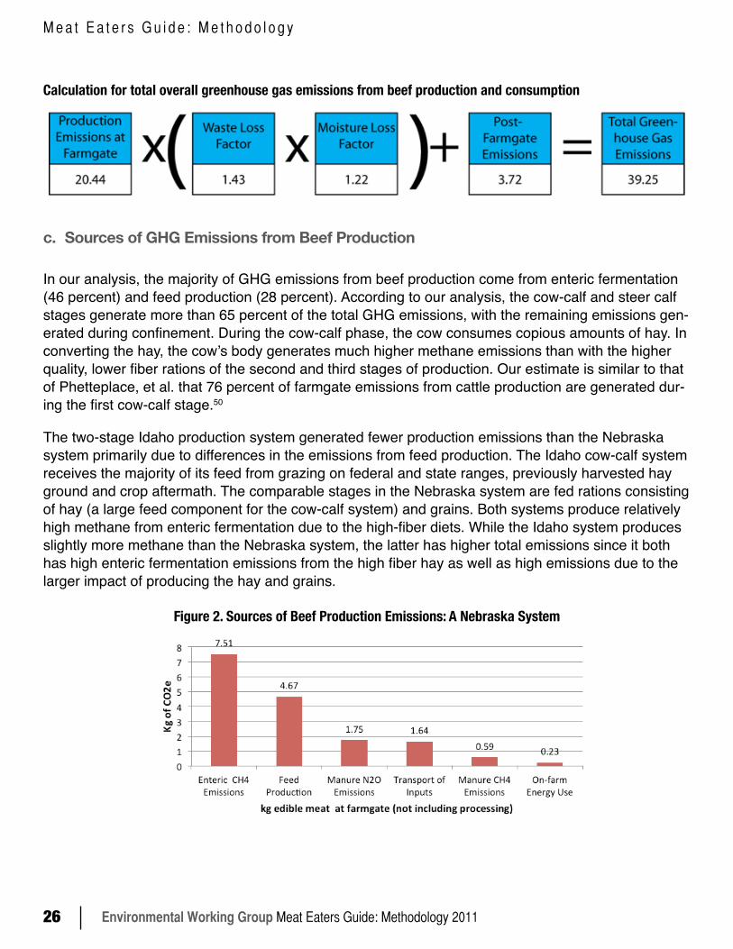
Calculation for total overall greenhouse gas emissions from beef production and consumption
c. Sources of GHG Emissions from Beef Production
In our analysis, the majority of GHG emissions from beef production come from enteric fermentation (46 percent) and feed production (28 percent). According to our analysis, the cow-calf and steer calf stages generate more than 65 percent of the total GHG emissions, with the remaining emissions gen-erated during confinement. During the cow-calf phase, the cow consumes copious amounts of hay. In converting the hay, the cow’s body generates much higher methane emissions than with the higher quality, lower fiber rations of the second and third stages of production. Our estimate is similar to that of Phetteplace, et al. that 76 percent of farmgate emissions from cattle production are generated dur-ing the first cow-calf stage.50
The two-stage Idaho production system generated fewer production emissions than the Nebraska system primarily due to differences in the emissions from feed production. The Idaho cow-calf system receives the majority of its feed from grazing on federal and state ranges, previously harvested hay ground and crop aftermath. The comparable stages in the Nebraska system are fed rations consisting of hay (a large feed component for the cow-calf system) and grains. Both systems produce relatively high methane from enteric fermentation due to the high-fiber diets. While the Idaho system produces slightly more methane than the Nebraska system, the latter has higher total emissions since it both has high enteric fermentation emissions from the high fiber hay as well as high emissions due to the larger impact of producing the hay and grains.
Figure 2. Sources of Beef Production Emissions: A Nebraska System
Environmental Working Group Meat Eaters Guide: Methodology 2011 27
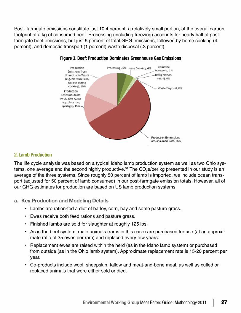
Post- farmgate emissions constitute just 10.4 percent, a relatively small portion, of the overall carbon footprint of a kg of consumed beef. Processing (including freezing) accounts for nearly half of post- farmgate beef emissions, but just 5 percent of total GHG emissions, followed by home cooking (4 percent), and domestic transport (1 percent) waste disposal (.3 percent).
Figure 3. Beef: Production Dominates Greenhouse Gas Emissions
2. Lamb Production The life cycle analysis was based on a typical Idaho lamb production system as well as two Ohio sys-tems, one average and the second highly productive.51 The CO2e/per kg presented in our study is an average of the three systems. Since roughly 50 percent of lamb is imported, we include ocean trans-port (adjusted for 50 percent of lamb consumed) in our post-farmgate emission totals. However, all of our GHG estimates for production are based on US lamb production systems.
a. Key Production and Modeling Details• Lambs are ration-fed a diet of barley, corn, hay and some pasture grass. • Ewes receive both feed rations and pasture grass.• Finished lambs are sold for slaughter at roughly 125 lbs.• As in the beef system, male animals (rams in this case) are purchased for use (at an approxi-
mate ratio of 35 ewes per ram) and replaced every few years.• Replacement ewes are raised within the herd (as in the Idaho lamb system) or purchased
from outside (as in the Ohio lamb system). Approximate replacement rate is 15-20 percent per year.
• Co-products include wool, sheepskin, tallow and meat-and-bone meal, as well as culled or replaced animals that were either sold or died.
Production Emmissions of Consumed Beef, 56%
Environmental Working Group Meat Eaters Guide: Methodology 201128
M e a t E a t e r s G u i d e : M e t h o d o l o g y
• Although water is used in the operation, the data source does not itemize the actual quantities of water used. Therefore, water is currently excluded at this stage of the model due to lack of data.
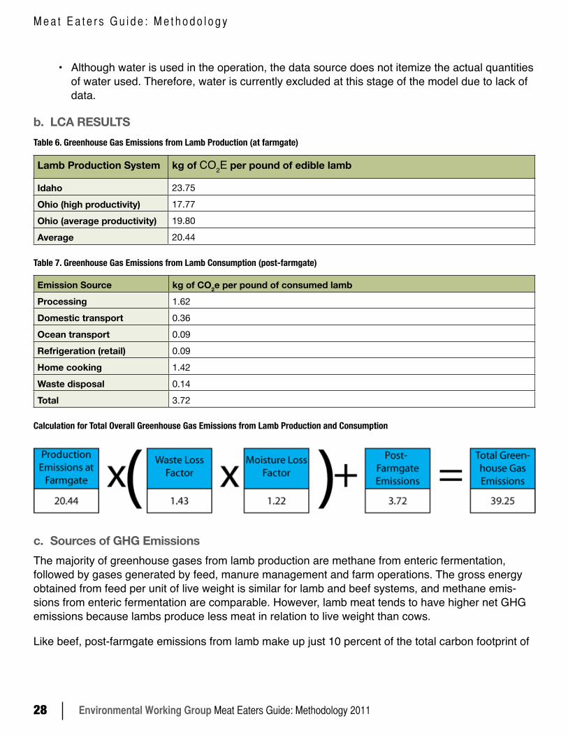
b. LCA RESULTSTable 6. Greenhouse Gas Emissions from Lamb Production (at farmgate)
Lamb Production System kg of CO2E per pound of edible lamb
Idaho 23.75
Ohio (high productivity) 17.77
Ohio (average productivity) 19.80
Average 20.44
Table 7. Greenhouse Gas Emissions from Lamb Consumption (post-farmgate)
Emission Source kg of CO2e per pound of consumed lambProcessing 1.62Domestic transport 0.36Ocean transport 0.09Refrigeration (retail) 0.09Home cooking 1.42Waste disposal 0.14Total 3.72
Calculation for Total Overall Greenhouse Gas Emissions from Lamb Production and Consumption
c. Sources of GHG EmissionsThe majority of greenhouse gases from lamb production are methane from enteric fermentation, followed by gases generated by feed, manure management and farm operations. The gross energy obtained from feed per unit of live weight is similar for lamb and beef systems, and methane emis-sions from enteric fermentation are comparable. However, lamb meat tends to have higher net GHG emissions because lambs produce less meat in relation to live weight than cows.
Like beef, post-farmgate emissions from lamb make up just 10 percent of the total carbon footprint of
Environmental Working Group Meat Eaters Guide: Methodology 2011 29
a kg of lamb. Processing (including freezing and packaging) accounts for 4 percent of total emissions, followed by home cooking (3 percent), and both waste disposal and domestic transport (less than 1 percent each).
3. Pork ProductionThe CleanMetrics LCA analysis modeled four typical single-stage pork production systems: two from Michigan (average- and high-productivity) and two from the country’s leading pork-producing state, Iowa. In once case, the animals have some pasture access, but the feed rations are similar in both confined and some pasture access.
a. Key Production and Modeling Details• One-stage system with sows and piglets raised together 52 • A pork system with pasture access uses nearly the same feed inputs (mostly corn, soybean
meal and other grains) as a confined system, since the animals do not obtain much nutrition from grazing on pasture.
• Manure management system is assumed to be liquid slurry with natural crust cover. Although some manure was deposited on pasture in the Iowa pasture system, the model does not separate that out due to lack of data.
• Fuel and electricity are main energy inputs for farm operation. (Energy used for delivering water is excluded due to lack of data).
• Hogs in each system are sold to slaughter at a weight of around 260 lbs • Transport assumptions are similar to beef and lamb systems.
b. LCA Results
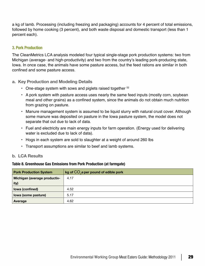
Table 8. Greenhouse Gas Emissions from Pork Production (at farmgate)
Pork Production System kg of CO2e per pound of edible porkMichigan (average productiv-ity)
4.17
Iowa (confined) 4.52
Iowa (some pasture) 5.17
Average 4.62
Environmental Working Group Meat Eaters Guide: Methodology 201130
M e a t E a t e r s G u i d e : M e t h o d o l o g y
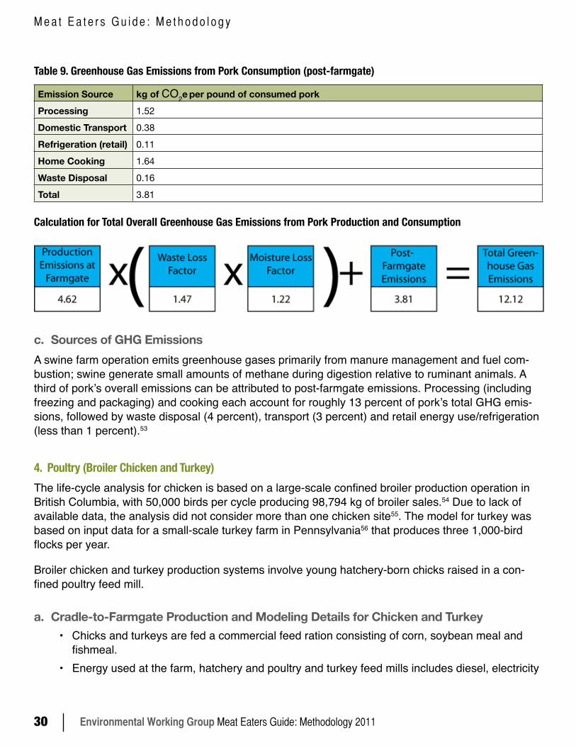
Table 9. Greenhouse Gas Emissions from Pork Consumption (post-farmgate)
Emission Source kg of CO2e per pound of consumed porkProcessing 1.52Domestic Transport 0.38Refrigeration (retail) 0.11Home Cooking 1.64Waste Disposal 0.16Total 3.81
Calculation for Total Overall Greenhouse Gas Emissions from Pork Production and Consumption
c. Sources of GHG EmissionsA swine farm operation emits greenhouse gases primarily from manure management and fuel com-bustion; swine generate small amounts of methane during digestion relative to ruminant animals. A third of pork’s overall emissions can be attributed to post-farmgate emissions. Processing (including freezing and packaging) and cooking each account for roughly 13 percent of pork’s total GHG emis-sions, followed by waste disposal (4 percent), transport (3 percent) and retail energy use/refrigeration (less than 1 percent).53
4. Poultry (Broiler Chicken and Turkey)The life-cycle analysis for chicken is based on a large-scale confined broiler production operation in British Columbia, with 50,000 birds per cycle producing 98,794 kg of broiler sales.54 Due to lack of available data, the analysis did not consider more than one chicken site55. The model for turkey was based on input data for a small-scale turkey farm in Pennsylvania56 that produces three 1,000-bird flocks per year.
Broiler chicken and turkey production systems involve young hatchery-born chicks raised in a con-fined poultry feed mill.
a. Cradle-to-Farmgate Production and Modeling Details for Chicken and Turkey• Chicks and turkeys are fed a commercial feed ration consisting of corn, soybean meal and
fishmeal. • Energy used at the farm, hatchery and poultry and turkey feed mills includes diesel, electricity
Environmental Working Group Meat Eaters Guide: Methodology 2011 31
and natural gas. Water is excluded due to lack of data.• Chicken slaughter weight is 6 lbs57
• Turkey slaughter weight is 15 lbs for hens and 30 lbs for toms.
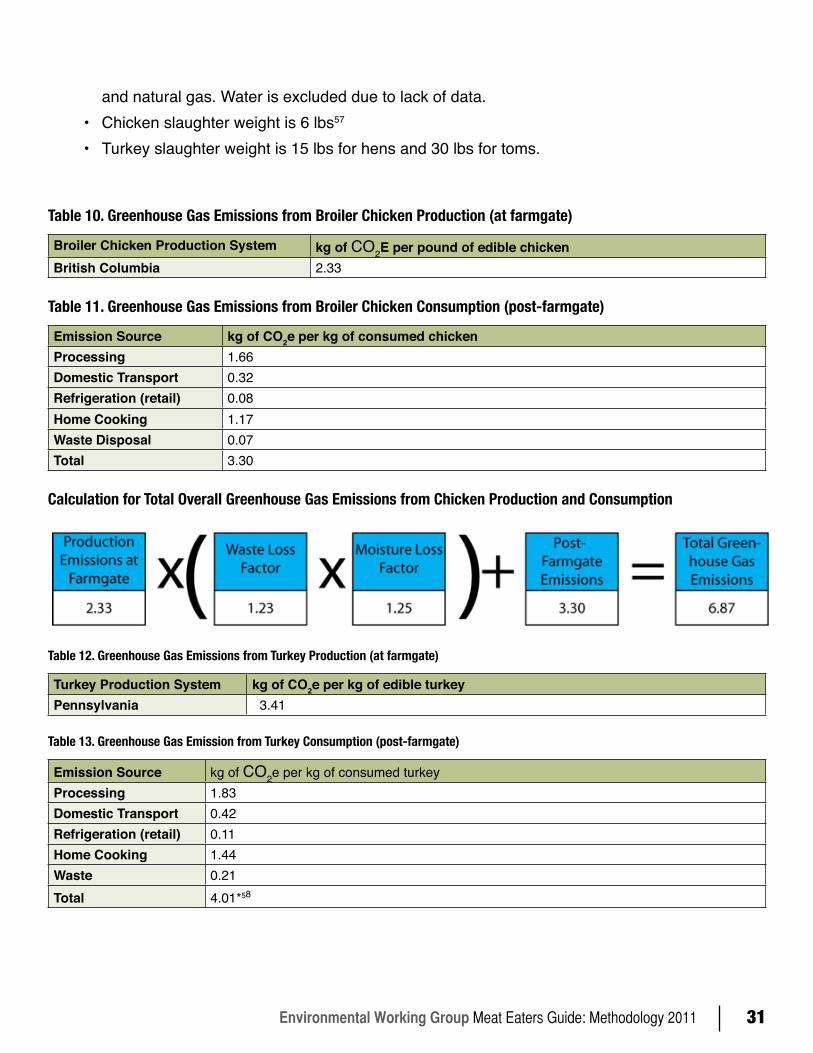
Table 10. Greenhouse Gas Emissions from Broiler Chicken Production (at farmgate)
Broiler Chicken Production System kg of CO2E per pound of edible chickenBritish Columbia 2.33
Table 11. Greenhouse Gas Emissions from Broiler Chicken Consumption (post-farmgate)
Emission Source kg of CO2e per kg of consumed chickenProcessing 1.66Domestic Transport 0.32Refrigeration (retail) 0.08Home Cooking 1.17Waste Disposal 0.07Total 3.30
Calculation for Total Overall Greenhouse Gas Emissions from Chicken Production and Consumption
Table 12. Greenhouse Gas Emissions from Turkey Production (at farmgate)
Turkey Production System kg of CO2e per kg of edible turkeyPennsylvania 3.41
Table 13. Greenhouse Gas Emission from Turkey Consumption (post-farmgate)
Emission Source kg of CO2e per kg of consumed turkeyProcessing 1.83Domestic Transport 0.42Refrigeration (retail) 0.11Home Cooking 1.44Waste 0.21Total 4.01*58
Environmental Working Group Meat Eaters Guide: Methodology 201132
M e a t E a t e r s G u i d e : M e t h o d o l o g y
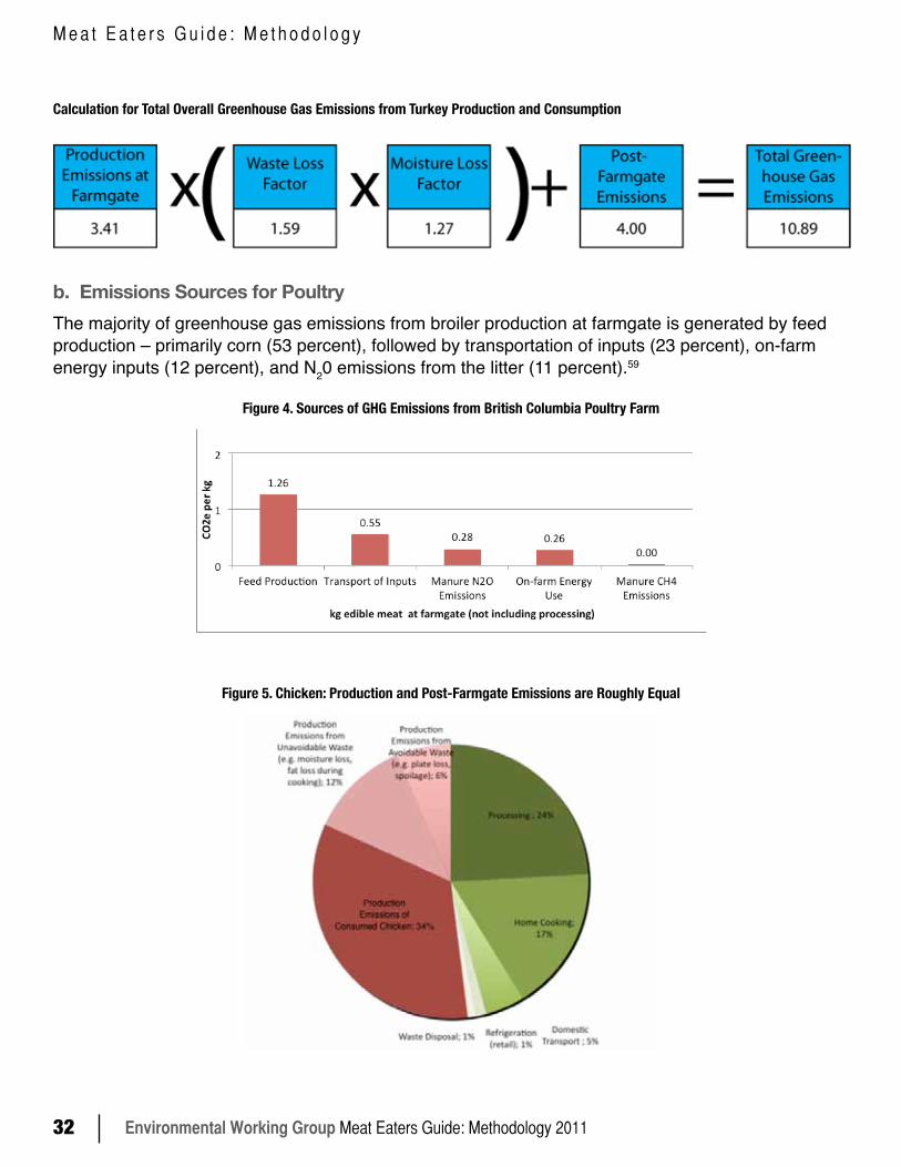
Calculation for Total Overall Greenhouse Gas Emissions from Turkey Production and Consumption
b. Emissions Sources for PoultryThe majority of greenhouse gas emissions from broiler production at farmgate is generated by feed production – primarily corn (53 percent), followed by transportation of inputs (23 percent), on-farm energy inputs (12 percent), and N20 emissions from the litter (11 percent).59
Figure 4. Sources of GHG Emissions from British Columbia Poultry Farm
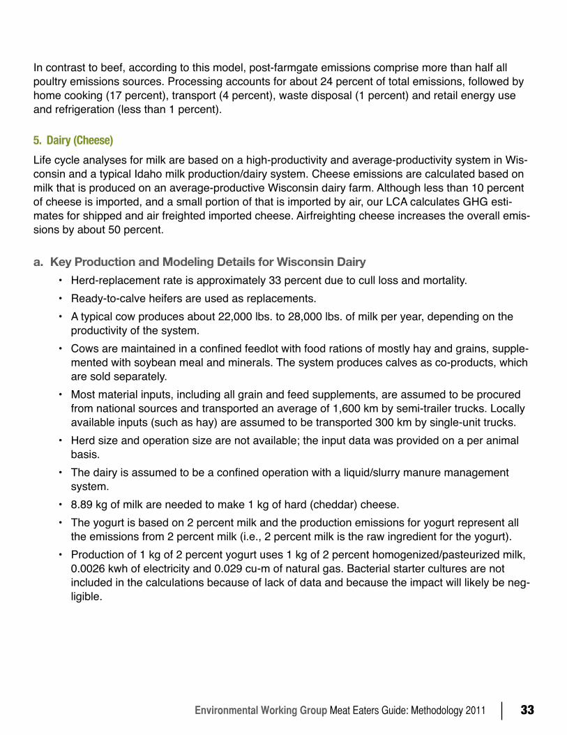
Figure 5. Chicken: Production and Post-Farmgate Emissions are Roughly Equal
Environmental Working Group Meat Eaters Guide: Methodology 2011 33
In contrast to beef, according to this model, post-farmgate emissions comprise more than half all poultry emissions sources. Processing accounts for about 24 percent of total emissions, followed by home cooking (17 percent), transport (4 percent), waste disposal (1 percent) and retail energy use and refrigeration (less than 1 percent).
5. Dairy (Cheese)Life cycle analyses for milk are based on a high-productivity and average-productivity system in Wis-consin and a typical Idaho milk production/dairy system. Cheese emissions are calculated based on milk that is produced on an average-productive Wisconsin dairy farm. Although less than 10 percent of cheese is imported, and a small portion of that is imported by air, our LCA calculates GHG esti-mates for shipped and air freighted imported cheese. Airfreighting cheese increases the overall emis-sions by about 50 percent.
a. Key Production and Modeling Details for Wisconsin Dairy• Herd-replacement rate is approximately 33 percent due to cull loss and mortality. • Ready-to-calve heifers are used as replacements. • A typical cow produces about 22,000 lbs. to 28,000 lbs. of milk per year, depending on the
productivity of the system. • Cows are maintained in a confined feedlot with food rations of mostly hay and grains, supple-
mented with soybean meal and minerals. The system produces calves as co-products, which are sold separately.
• Most material inputs, including all grain and feed supplements, are assumed to be procured from national sources and transported an average of 1,600 km by semi-trailer trucks. Locally available inputs (such as hay) are assumed to be transported 300 km by single-unit trucks.
• Herd size and operation size are not available; the input data was provided on a per animal basis.
• The dairy is assumed to be a confined operation with a liquid/slurry manure management system.
• 8.89 kg of milk are needed to make 1 kg of hard (cheddar) cheese.• The yogurt is based on 2 percent milk and the production emissions for yogurt represent all
the emissions from 2 percent milk (i.e., 2 percent milk is the raw ingredient for the yogurt). • Production of 1 kg of 2 percent yogurt uses 1 kg of 2 percent homogenized/pasteurized milk,
0.0026 kwh of electricity and 0.029 cu-m of natural gas. Bacterial starter cultures are not included in the calculations because of lack of data and because the impact will likely be neg-ligible.
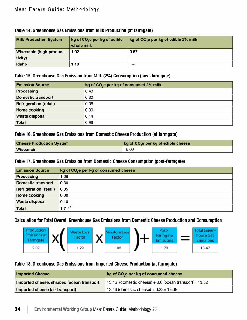
Environmental Working Group Meat Eaters Guide: Methodology 201134
M e a t E a t e r s G u i d e : M e t h o d o l o g y
Table 14. Greenhouse Gas Emissions from Milk Production (at farmgate)
Milk Production System kg of CO2e per kg of edible whole milk
kg of CO2e per kg of edible 2% milk
Wisconsin (high produc-tivity)
1.02 0.67
Idaho 1.10 --
Table 15. Greenhouse Gas Emission from Milk (2%) Consumption (post-farmgate)
Emission Source kg of CO2e per kg of consumed 2% milkProcessing 0.48Domestic transport 0.30Refrigeration (retail) 0.06Home cooking 0.00Waste disposal 0.14Total 0.98
Table 16. Greenhouse Gas Emissions from Domestic Cheese Production (at farmgate)
Cheese Production System kg of CO2e per kg of edible cheeseWisconsin 9.09
Table 17. Greenhouse Gas Emission from Domestic Cheese Consumption (post-farmgate)
Emission Source kg of CO2e per kg of consumed cheeseProcessing 1.26Domestic transport 0.30Refrigeration (retail) 0.05Home cooking 0.00Waste disposal 0.10Total 1.7162
Calculation for Total Overall Greenhouse Gas Emissions from Domestic Cheese Production and Consumption
Table 18. Greenhouse Gas Emissions from Imported Cheese Production (at farmgate)
Imported Cheese kg of CO2e per kg of consumed cheese
Imported cheese, shipped (ocean transport 13.46 (domestic cheese) + .06 (ocean transport)= 13.52
Imported cheese (air transport) 13.46 (domestic cheese) + 6.22= 19.68
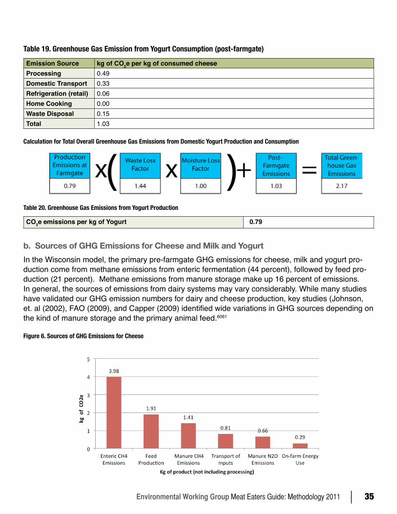
Environmental Working Group Meat Eaters Guide: Methodology 2011 35
Table 19. Greenhouse Gas Emission from Yogurt Consumption (post-farmgate)
Emission Source kg of CO2e per kg of consumed cheeseProcessing 0.49Domestic Transport 0.33Refrigeration (retail) 0.06Home Cooking 0.00Waste Disposal 0.15Total 1.03
Calculation for Total Overall Greenhouse Gas Emissions from Domestic Yogurt Production and Consumption
Table 20. Greenhouse Gas Emissions from Yogurt Production
CO2e emissions per kg of Yogurt 0.79
b. Sources of GHG Emissions for Cheese and Milk and YogurtIn the Wisconsin model, the primary pre-farmgate GHG emissions for cheese, milk and yogurt pro-duction come from methane emissions from enteric fermentation (44 percent), followed by feed pro-duction (21 percent). Methane emissions from manure storage make up 16 percent of emissions. In general, the sources of emissions from dairy systems may vary considerably. While many studies have validated our GHG emission numbers for dairy and cheese production, key studies (Johnson, et. al (2002), FAO (2009), and Capper (2009) identified wide variations in GHG sources depending on the kind of manure storage and the primary animal feed.6061
Figure 6. Sources of GHG Emissions for Cheese
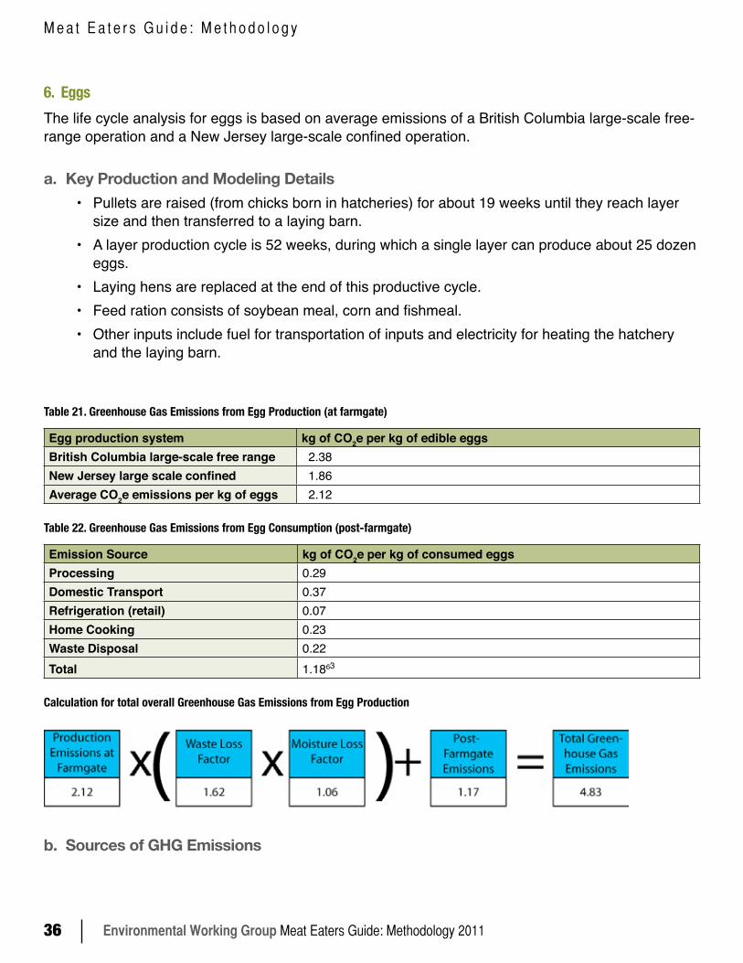
Environmental Working Group Meat Eaters Guide: Methodology 201136
M e a t E a t e r s G u i d e : M e t h o d o l o g y
6. EggsThe life cycle analysis for eggs is based on average emissions of a British Columbia large-scale free-range operation and a New Jersey large-scale confined operation.
a. Key Production and Modeling Details• Pullets are raised (from chicks born in hatcheries) for about 19 weeks until they reach layer
size and then transferred to a laying barn. • A layer production cycle is 52 weeks, during which a single layer can produce about 25 dozen
eggs. • Laying hens are replaced at the end of this productive cycle. • Feed ration consists of soybean meal, corn and fishmeal.• Other inputs include fuel for transportation of inputs and electricity for heating the hatchery
and the laying barn.
Table 21. Greenhouse Gas Emissions from Egg Production (at farmgate)
Egg production system kg of CO2e per kg of edible eggsBritish Columbia large-scale free range 2.38 New Jersey large scale confined 1.86 Average CO2e emissions per kg of eggs 2.12
Table 22. Greenhouse Gas Emissions from Egg Consumption (post-farmgate)
Emission Source kg of CO2e per kg of consumed eggsProcessing 0.29Domestic Transport 0.37Refrigeration (retail) 0.07Home Cooking 0.23Waste Disposal 0.22Total 1.1863
Calculation for total overall Greenhouse Gas Emissions from Egg Production
b. Sources of GHG Emissions
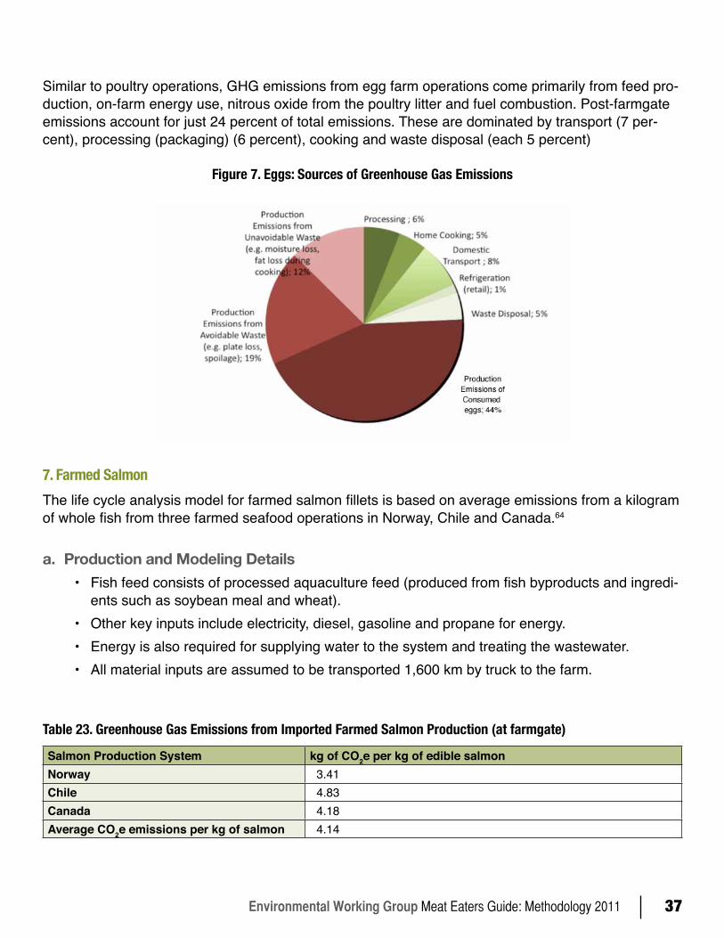
Environmental Working Group Meat Eaters Guide: Methodology 2011 37
Similar to poultry operations, GHG emissions from egg farm operations come primarily from feed pro-duction, on-farm energy use, nitrous oxide from the poultry litter and fuel combustion. Post-farmgate emissions account for just 24 percent of total emissions. These are dominated by transport (7 per-cent), processing (packaging) (6 percent), cooking and waste disposal (each 5 percent)
Figure 7. Eggs: Sources of Greenhouse Gas Emissions
7. Farmed SalmonThe life cycle analysis model for farmed salmon fillets is based on average emissions from a kilogram of whole fish from three farmed seafood operations in Norway, Chile and Canada.64
a. Production and Modeling Details• Fish feed consists of processed aquaculture feed (produced from fish byproducts and ingredi-
ents such as soybean meal and wheat). • Other key inputs include electricity, diesel, gasoline and propane for energy.• Energy is also required for supplying water to the system and treating the wastewater.• All material inputs are assumed to be transported 1,600 km by truck to the farm.
Table 23. Greenhouse Gas Emissions from Imported Farmed Salmon Production (at farmgate)
Salmon Production System kg of CO2e per kg of edible salmonNorway 3.41Chile 4.83 Canada 4.18Average CO2e emissions per kg of salmon 4.14
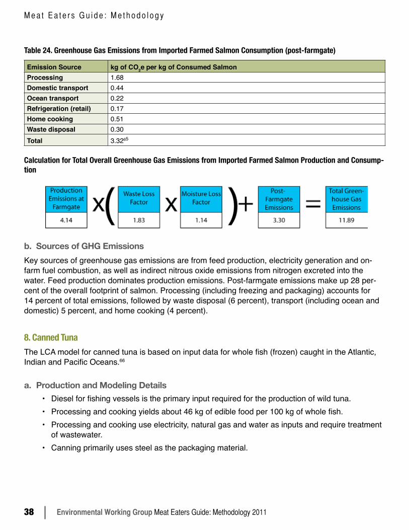
Environmental Working Group Meat Eaters Guide: Methodology 201138
M e a t E a t e r s G u i d e : M e t h o d o l o g y
Table 24. Greenhouse Gas Emissions from Imported Farmed Salmon Consumption (post-farmgate)
Emission Source kg of CO2e per kg of Consumed SalmonProcessing 1.68Domestic transport 0.44Ocean transport 0.22Refrigeration (retail) 0.17Home cooking 0.51Waste disposal 0.30Total 3.3265
Calculation for Total Overall Greenhouse Gas Emissions from Imported Farmed Salmon Production and Consump-tion
b. Sources of GHG Emissions Key sources of greenhouse gas emissions are from feed production, electricity generation and on-farm fuel combustion, as well as indirect nitrous oxide emissions from nitrogen excreted into the water. Feed production dominates production emissions. Post-farmgate emissions make up 28 per-cent of the overall footprint of salmon. Processing (including freezing and packaging) accounts for 14 percent of total emissions, followed by waste disposal (6 percent), transport (including ocean and domestic) 5 percent, and home cooking (4 percent).
8. Canned TunaThe LCA model for canned tuna is based on input data for whole fish (frozen) caught in the Atlantic, Indian and Pacific Oceans.66
a. Production and Modeling Details• Diesel for fishing vessels is the primary input required for the production of wild tuna.• Processing and cooking yields about 46 kg of edible food per 100 kg of whole fish.• Processing and cooking use electricity, natural gas and water as inputs and require treatment
of wastewater.• Canning primarily uses steel as the packaging material.
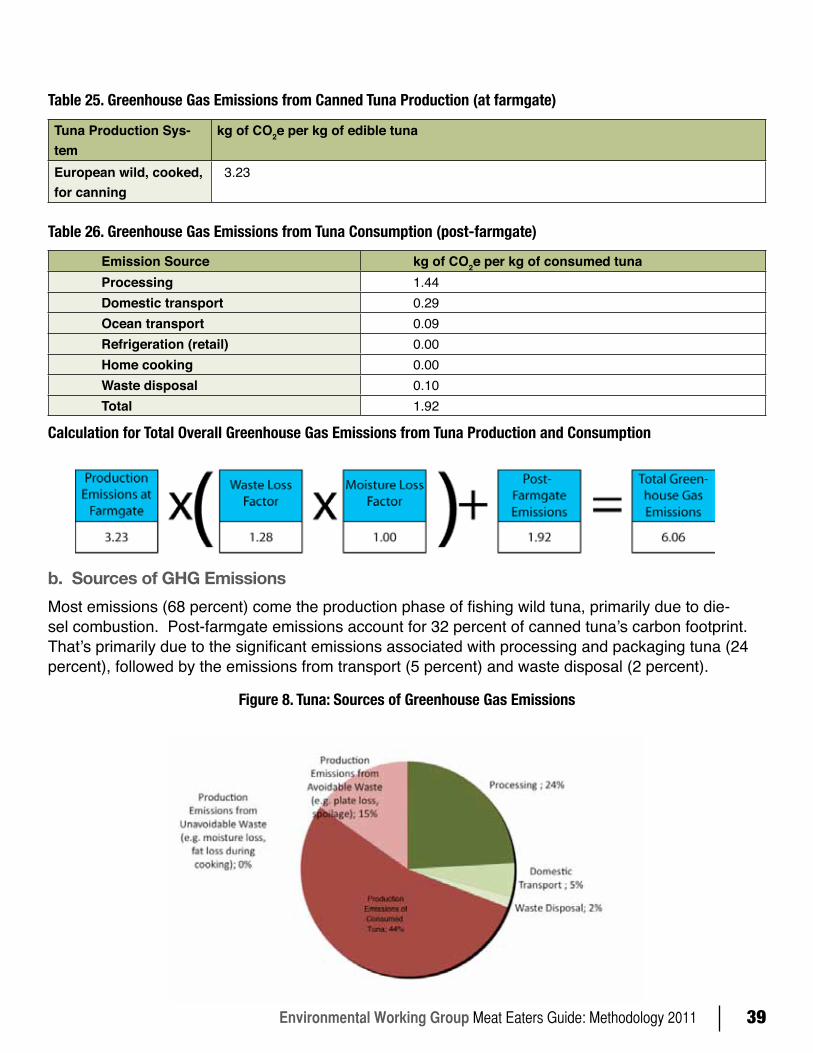
Environmental Working Group Meat Eaters Guide: Methodology 2011 39
Table 25. Greenhouse Gas Emissions from Canned Tuna Production (at farmgate)
Tuna Production Sys-tem
kg of CO2e per kg of edible tuna
European wild, cooked, for canning
3.23
Table 26. Greenhouse Gas Emissions from Tuna Consumption (post-farmgate)
Emission Source kg of CO2e per kg of consumed tunaProcessing 1.44Domestic transport 0.29Ocean transport 0.09Refrigeration (retail) 0.00Home cooking 0.00Waste disposal 0.10Total 1.92
Calculation for Total Overall Greenhouse Gas Emissions from Tuna Production and Consumption
b. Sources of GHG EmissionsMost emissions (68 percent) come the production phase of fishing wild tuna, primarily due to die-sel combustion. Post-farmgate emissions account for 32 percent of canned tuna’s carbon footprint. That’s primarily due to the significant emissions associated with processing and packaging tuna (24 percent), followed by the emissions from transport (5 percent) and waste disposal (2 percent).
Figure 8. Tuna: Sources of Greenhouse Gas Emissions
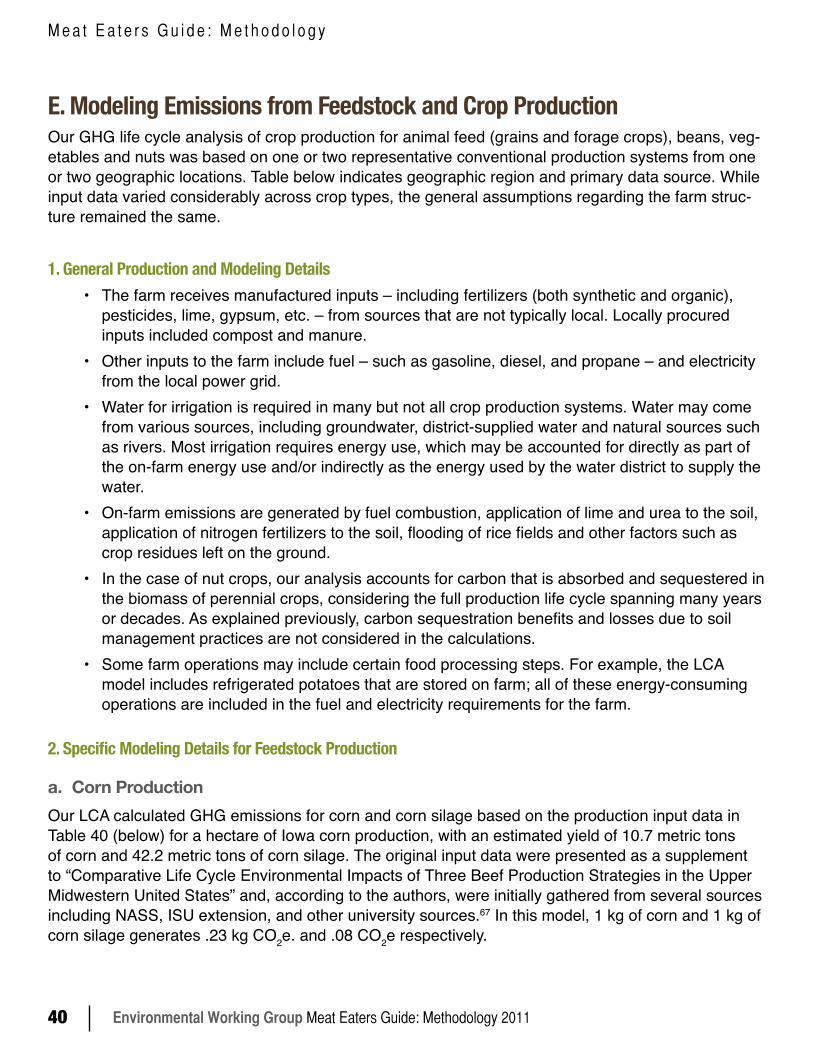
Environmental Working Group Meat Eaters Guide: Methodology 201140
M e a t E a t e r s G u i d e : M e t h o d o l o g y
E. Modeling Emissions from Feedstock and Crop ProductionOur GHG life cycle analysis of crop production for animal feed (grains and forage crops), beans, veg-etables and nuts was based on one or two representative conventional production systems from one or two geographic locations. Table below indicates geographic region and primary data source. While input data varied considerably across crop types, the general assumptions regarding the farm struc-ture remained the same.
1. General Production and Modeling Details• The farm receives manufactured inputs – including fertilizers (both synthetic and organic),
pesticides, lime, gypsum, etc. – from sources that are not typically local. Locally procured inputs included compost and manure.
• Other inputs to the farm include fuel – such as gasoline, diesel, and propane – and electricity from the local power grid.
• Water for irrigation is required in many but not all crop production systems. Water may come from various sources, including groundwater, district-supplied water and natural sources such as rivers. Most irrigation requires energy use, which may be accounted for directly as part of the on-farm energy use and/or indirectly as the energy used by the water district to supply the water.
• On-farm emissions are generated by fuel combustion, application of lime and urea to the soil, application of nitrogen fertilizers to the soil, flooding of rice fields and other factors such as crop residues left on the ground.
• In the case of nut crops, our analysis accounts for carbon that is absorbed and sequestered in the biomass of perennial crops, considering the full production life cycle spanning many years or decades. As explained previously, carbon sequestration benefits and losses due to soil management practices are not considered in the calculations.
• Some farm operations may include certain food processing steps. For example, the LCA model includes refrigerated potatoes that are stored on farm; all of these energy-consuming operations are included in the fuel and electricity requirements for the farm.
2. Specific Modeling Details for Feedstock Production
a. Corn ProductionOur LCA calculated GHG emissions for corn and corn silage based on the production input data in Table 40 (below) for a hectare of Iowa corn production, with an estimated yield of 10.7 metric tons of corn and 42.2 metric tons of corn silage. The original input data were presented as a supplement to “Comparative Life Cycle Environmental Impacts of Three Beef Production Strategies in the Upper Midwestern United States” and, according to the authors, were initially gathered from several sources including NASS, ISU extension, and other university sources.67 In this model, 1 kg of corn and 1 kg of corn silage generates .23 kg CO2e. and .08 CO2e respectively.
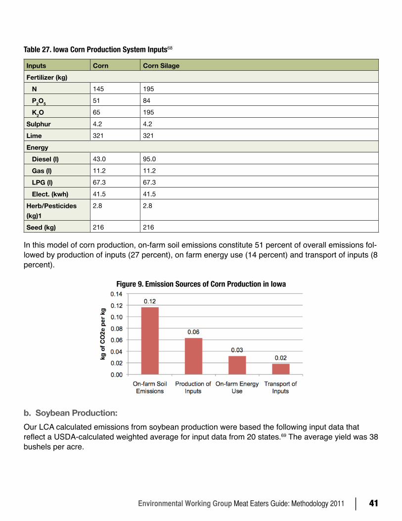
Environmental Working Group Meat Eaters Guide: Methodology 2011 41
Table 27. Iowa Corn Production System Inputs68
Inputs Corn Corn SilageFertilizer (kg) N 145 195
P2O5 51 84
K2O 65 195
Sulphur 4.2 4.2
Lime 321 321
Energy Diesel (l) 43.0 95.0
Gas (l) 11.2 11.2
LPG (l) 67.3 67.3
Elect. (kwh) 41.5 41.5
Herb/Pesticides (kg)1
2.8 2.8
Seed (kg) 216 216
In this model of corn production, on-farm soil emissions constitute 51 percent of overall emissions fol-lowed by production of inputs (27 percent), on farm energy use (14 percent) and transport of inputs (8 percent).
Figure 9. Emission Sources of Corn Production in Iowa
b. Soybean Production:Our LCA calculated emissions from soybean production were based the following input data that reflect a USDA-calculated weighted average for input data from 20 states.69 The average yield was 38 bushels per acre.
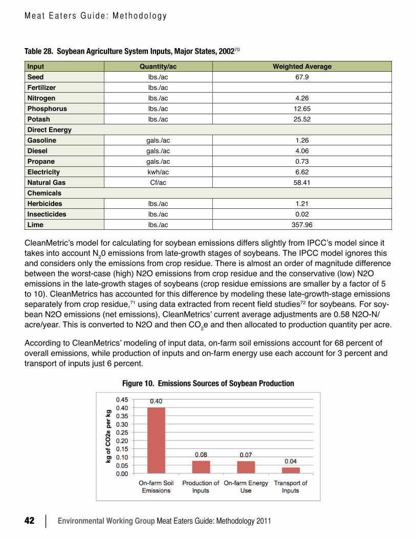
Environmental Working Group Meat Eaters Guide: Methodology 201142
M e a t E a t e r s G u i d e : M e t h o d o l o g y
Table 28. Soybean Agriculture System Inputs, Major States, 200270
Input Quantity/ac Weighted AverageSeed lbs./ac 67.9Fertilizer lbs./acNitrogen lbs./ac 4.26Phosphorus lbs./ac 12.65Potash lbs./ac 25.52Direct EnergyGasoline gals./ac 1.26Diesel gals./ac 4.06Propane gals./ac 0.73Electricity kwh/ac 6.62Natural Gas Cf/ac 58.41ChemicalsHerbicides lbs./ac 1.21Insecticides lbs./ac 0.02Lime lbs./ac 357.96
CleanMetric’s model for calculating for soybean emissions differs slightly from IPCC’s model since it takes into account N20 emissions from late-growth stages of soybeans. The IPCC model ignores this and considers only the emissions from crop residue. There is almost an order of magnitude difference between the worst-case (high) N2O emissions from crop residue and the conservative (low) N2O emissions in the late-growth stages of soybeans (crop residue emissions are smaller by a factor of 5 to 10). CleanMetrics has accounted for this difference by modeling these late-growth-stage emissions separately from crop residue,71 using data extracted from recent field studies72 for soybeans. For soy-bean N2O emissions (net emissions), CleanMetrics’ current average adjustments are 0.58 N2O-N/acre/year. This is converted to N2O and then CO2e and then allocated to production quantity per acre.
According to CleanMetrics’ modeling of input data, on-farm soil emissions account for 68 percent of overall emissions, while production of inputs and on-farm energy use each account for 3 percent and transport of inputs just 6 percent.
Figure 10. Emissions Sources of Soybean Production
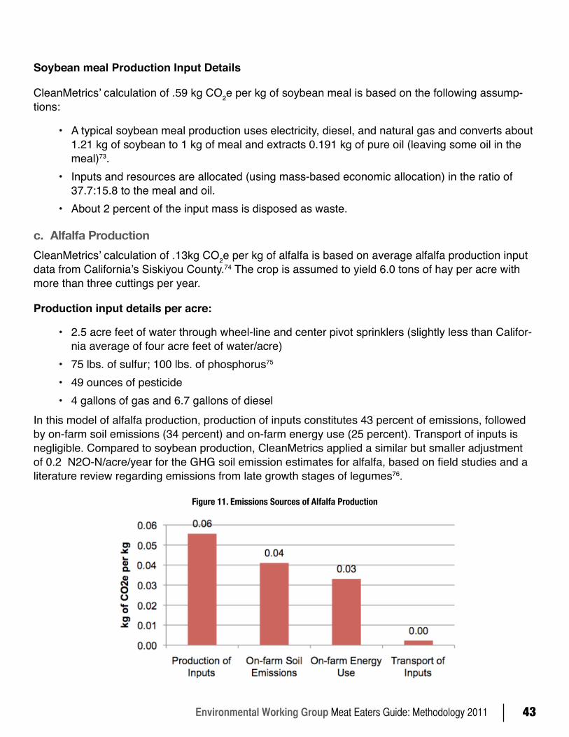
Environmental Working Group Meat Eaters Guide: Methodology 2011 43
Soybean meal Production Input Details
CleanMetrics’ calculation of .59 kg CO2e per kg of soybean meal is based on the following assump-tions:
• A typical soybean meal production uses electricity, diesel, and natural gas and converts about 1.21 kg of soybean to 1 kg of meal and extracts 0.191 kg of pure oil (leaving some oil in the meal)73.
• Inputs and resources are allocated (using mass-based economic allocation) in the ratio of 37.7:15.8 to the meal and oil.
• About 2 percent of the input mass is disposed as waste.
c. Alfalfa ProductionCleanMetrics’ calculation of .13kg CO2e per kg of alfalfa is based on average alfalfa production input data from California’s Siskiyou County.74 The crop is assumed to yield 6.0 tons of hay per acre with more than three cuttings per year.
Production input details per acre:
• 2.5 acre feet of water through wheel-line and center pivot sprinklers (slightly less than Califor-nia average of four acre feet of water/acre)
• 75 lbs. of sulfur; 100 lbs. of phosphorus75 • 49 ounces of pesticide • 4 gallons of gas and 6.7 gallons of diesel
In this model of alfalfa production, production of inputs constitutes 43 percent of emissions, followed by on-farm soil emissions (34 percent) and on-farm energy use (25 percent). Transport of inputs is negligible. Compared to soybean production, CleanMetrics applied a similar but smaller adjustment of 0.2 N2O-N/acre/year for the GHG soil emission estimates for alfalfa, based on field studies and a literature review regarding emissions from late growth stages of legumes76.
Figure 11. Emissions Sources of Alfalfa Production
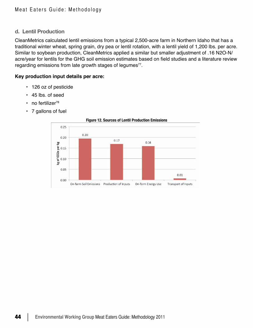
Environmental Working Group Meat Eaters Guide: Methodology 201144
M e a t E a t e r s G u i d e : M e t h o d o l o g y
d. Lentil ProductionCleanMetrics calculated lentil emissions from a typical 2,500-acre farm in Northern Idaho that has a traditional winter wheat, spring grain, dry pea or lentil rotation, with a lentil yield of 1,200 lbs. per acre. Similar to soybean production, CleanMetrics applied a similar but smaller adjustment of .16 N2O-N/acre/year for lentils for the GHG soil emission estimates based on field studies and a literature review regarding emissions from late growth stages of legumes77.
Key production input details per acre:
• 126 oz of pesticide• 45 lbs. of seed• no fertilizer78
• 7 gallons of fuelFigure 12. Sources of Lentil Production Emissions
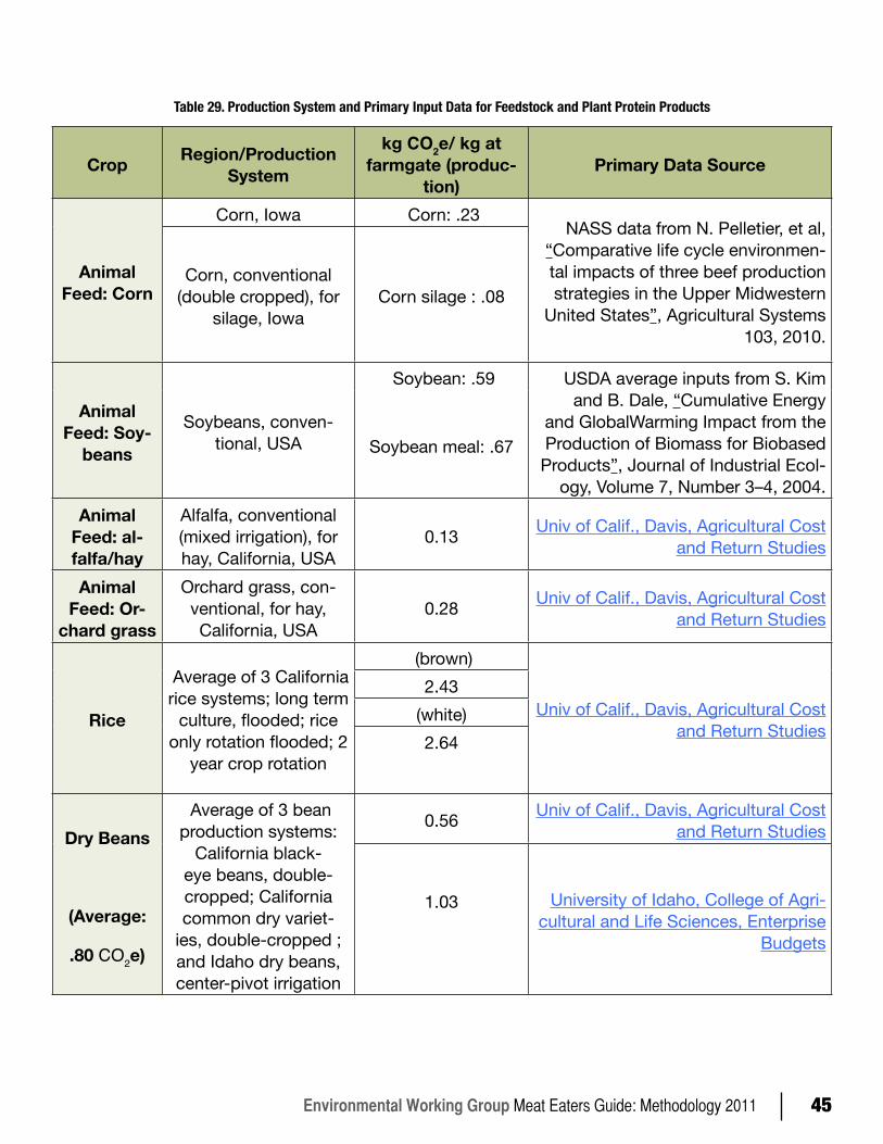
Environmental Working Group Meat Eaters Guide: Methodology 2011 45
Table 29. Production System and Primary Input Data for Feedstock and Plant Protein Products
Crop Region/Production System
kg CO2e/ kg at farmgate (produc-
tion)Primary Data Source
Animal Feed: Corn
Corn, Iowa Corn: .23NASS data from N. Pelletier, et al,
“Comparative life cycle environmen-tal impacts of three beef production strategies in the Upper Midwestern
United States”, Agricultural Systems 103, 2010.
Corn, conventional (double cropped), for
silage, IowaCorn silage : .08
Animal Feed: Soy-
beans
Soybeans, conven-tional, USA
Soybean: .59 USDA average inputs from S. Kim and B. Dale, “Cumulative Energy
and GlobalWarming Impact from the Production of Biomass for Biobased Products”, Journal of Industrial Ecol-
ogy, Volume 7, Number 3–4, 2004.
Soybean meal: .67
Animal Feed: al-falfa/hay
Alfalfa, conventional (mixed irrigation), for hay, California, USA
0.13 Univ of Calif., Davis, Agricultural Cost and Return Studies
Animal Feed: Or-
chard grass
Orchard grass, con-ventional, for hay, California, USA
0.28 Univ of Calif., Davis, Agricultural Cost and Return Studies
Rice
Average of 3 California rice systems; long term
culture, flooded; rice only rotation flooded; 2
year crop rotation
(brown)
Univ of Calif., Davis, Agricultural Cost and Return Studies
2.43(white)2.64
Dry Beans
(Average:
.80 CO2e)
Average of 3 bean production systems:
California black-eye beans, double-cropped; California common dry variet-
ies, double-cropped ; and Idaho dry beans, center-pivot irrigation
0.56 Univ of Calif., Davis, Agricultural Cost and Return Studies
1.03 University of Idaho, College of Agri-cultural and Life Sciences, Enterprise
Budgets
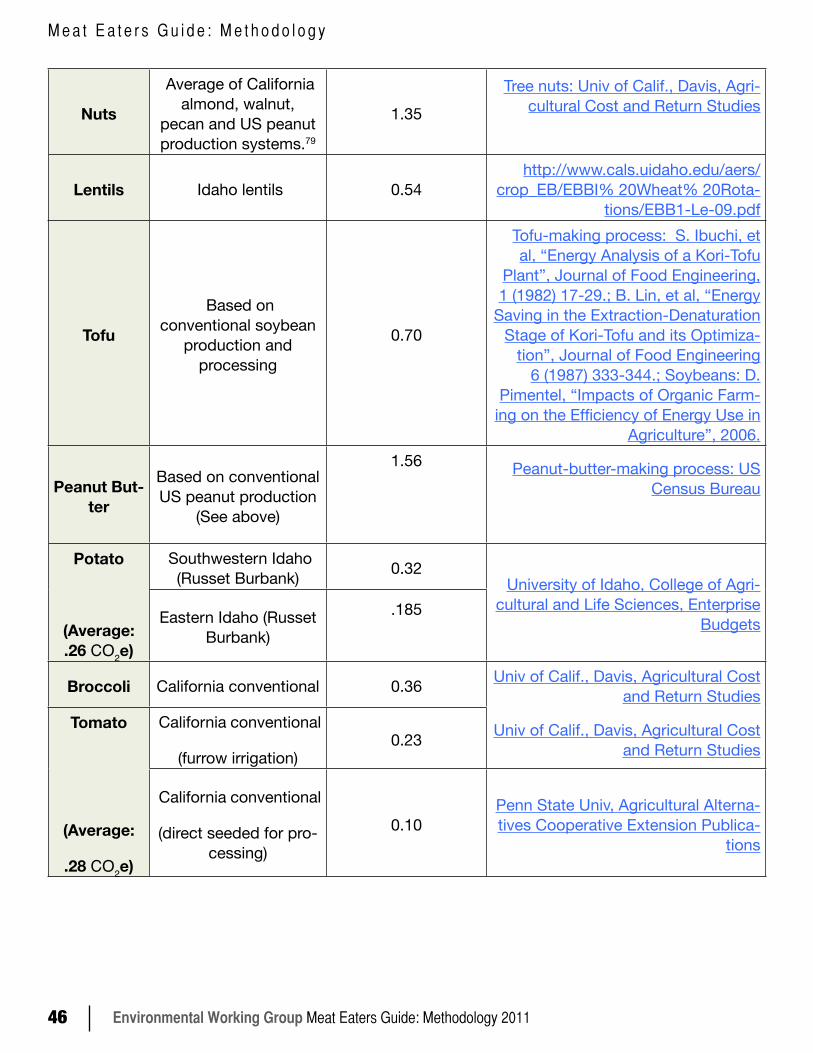
Environmental Working Group Meat Eaters Guide: Methodology 201146
M e a t E a t e r s G u i d e : M e t h o d o l o g y
Nuts
Average of California almond, walnut,
pecan and US peanut production systems.79
1.35Tree nuts: Univ of Calif., Davis, Agri-
cultural Cost and Return Studies
Lentils Idaho lentils 0.54http://www.cals.uidaho.edu/aers/
crop_EB/EBBI% 20Wheat% 20Rota-tions/EBB1-Le-09.pdf
Tofu
Based on conventional soybean
production and processing
0.70
Tofu-making process: S. Ibuchi, et al, “Energy Analysis of a Kori-Tofu
Plant”, Journal of Food Engineering, 1 (1982) 17-29.; B. Lin, et al, “Energy
Saving in the Extraction-Denaturation Stage of Kori-Tofu and its Optimiza-
tion”, Journal of Food Engineering 6 (1987) 333-344.; Soybeans: D.
Pimentel, “Impacts of Organic Farm-ing on the Efficiency of Energy Use in
Agriculture”, 2006.
Peanut But-ter
Based on conventional US peanut production
(See above)
1.56
Peanut-butter-making process: US Census Bureau
Potato
(Average: .26 CO2e)
Southwestern Idaho (Russet Burbank) 0.32
University of Idaho, College of Agri-cultural and Life Sciences, Enterprise
BudgetsEastern Idaho (Russet Burbank)
.185
Broccoli California conventional 0.36 Univ of Calif., Davis, Agricultural Cost and Return Studies
Tomato
(Average:
.28 CO2e)
California conventional
(furrow irrigation)0.23 Univ of Calif., Davis, Agricultural Cost
and Return Studies
California conventional
(direct seeded for pro-cessing)
0.10Penn State Univ, Agricultural Alterna-tives Cooperative Extension Publica-
tions
Environmental Working Group Meat Eaters Guide: Methodology 2011 47
3. Sources of Emissions of Plant ProteinIn contrast to meat proteins, plant proteins have much higher emissions associated with the post-farmgate phase, as opposed to production activities. For major plant proteins such as dry beans and lentils, post-farmgate emissions represent 65 and 59 percent of total emissions. Potatoes are highest, with 90 percent of emissions attributed to post-farmgate activities. Most of these emissions come from the energy used in cooking. In the case of dry beans, for example, home cooking generates slightly higher emissions than the actual production process of the beans. Generally speaking the second largest contributor of post-farmgate emissions is transport, followed by waste disposal.
Endnotes1. The analysis drew from CleanMetrics’ extensive life-cycle inventory database of agriculture, food produc-
tion and processing inputs and energy sources.
2. The greenhouse gas (GHG) emissions are calculated in terms of carbon dioxide equivalents (CO2e), incor-porating carbon dioxide emissions as well as the 100-year global warming potentials of other GHGs such as methane and nitrous oxide.
3. For instance, recent research commissioned by the USDA shows that 22 percent of the weight of pack-aged beef is never used, or it is wasted during cooking or disposed of after a meal. Therefore, we calculate that it will take 1.59 kgs of beef to produce 1kg of edible meat at farmgate; thus for every kg of meat that is consumed we attribute GHGs to 1.59kg of meat produced. This same model calculates that .59 kgs is lost during the retail and consumption phase.
4. IPCC Fourth Assessment Report: Climate Change 2007 2.10.2 Direct Global Warming Potentials accessed 18 January 2011 at http://www.ipcc.ch/publications_and_data/ar4/wg1/en/ch2s2-10-2.html
5. Our model calculates pre-farmgate emissions and post-farmgate emissions. Pre-farmgate refers to all the inputs and outputs associated with the production of a kg of product before it leaves the farm. Post- farm-gate refers to everything that occurs after it leaves the farm (e.g. processing, , freezing, packaging, retail refrigeration, transport, cooking and waste disposal)
6. For additional background info on allocation, see for example, N. Ayer et al. “Co-product allocation in life cycle assessments of seafood production systems: Review of problems and strategies”. International Jour-nal of Life Cycle Assessment 12 (7) 480 – 487 (2007).
7. In the “recycled content” method, the costs and benefits of the recycling are allocated to product systems that use the recycled material in some form. See further description at the Inventory of Carbon and Energy website (http://people.bath.ac.uk/cj219/ice00a.pdf)
8. Soil carbon sequestration is not accounted for in this model based on the IPPC guidance and generally accepted assumption used in LCA that all production systems under consideration have reached steady
Environmental Working Group Meat Eaters Guide: Methodology 201148
M e a t E a t e r s G u i d e : M e t h o d o l o g y
states where the net carbon flux from the soil is zero on average (spatial/temporal average). it should be pointed out that assumptions about steady state remain the subject of considerable scientific debate.
9. Manure benefits go to crop systems that use it as fertilizer, per the “recycled content” method. No benefits are accounted for in the animal system that produces the manure. No change to soil carbon stock in crop systems that use the manure -- under the assumption that the system is at steady state and the net soil carbon flux is zero on average.
10. While some homes will use electricity for cooking, our model assumes the use of natural gas; further cook-ing assumptions are included in Annex B.
11. The size of the large-scale operation is 50,000 birds, smaller than the typical 200,000 in a US poultry op-eration.
12. While a significant portion of fertilizer is imported and shipped to the United States, emissions from ship-ping a minor portion of overall emissions from fertilizer production and delivery. For freight transport by ocean where the product is not under temperature control, the road transport on either side of the ocean segment generally dominates the total transport emissions. For example, for 1 Kg of state-of-the-art nitro-gen fertilizer transported 5000 km by ocean and 1600 km by semi-trailer truck, the ocean transport con-tributes about 1.3% of the total fertilizer-related emissions at the point of delivery to a farm while the truck transport contributes 9.1%.
13. We assumed these nominal transport distances for inputs because most agricultural production data sources do not provide this information. We tested the sensitivities of our assumptions and found that the final results are quite insensitive to these assumptions. For example, in the case of corn produced in the Midwest, if the input transport distances changed by +/-25% relative to our assumptions, the cradle-to-farmgate emissions would change by less than 2 percent (even less if you consider the emissions as a total percentage of cradle to grave emissions). Transport-related emissions are generally a very minor compo-nent of the overall GHG emissions per Kg of product.
14. Fertilizer production is modeled uniformly on current state-of-the-art technologies per the International Fer-tilizer Association and is not country-specific.
15. While many animals are transported far greater distances from their original grazing or confined pasture lands, we used this distance since our models were based on regional production systems in which all sub-systems (such as cow-calf and feedlot) are in the same state. The sensitivity of final results to this assump-tion is very low. The 300 km transport adds less than 0.1 Kg CO2e to the cradle-to-gate GHG emissions of 1 Kg of meat. If we increase this to 1,500 km, it would still represent a very small portion of the overall carbon footprint.
16. The number was selected somewhat arbitrarily based on average distances from the middle of the country, where a majority of meat is produced, to major populations centers on either coast.
Environmental Working Group Meat Eaters Guide: Methodology 2011 49
17. Fertilizer production is modeled uniformly based on current state-of-the-art technologies per the Internation-al Fertilizer Association and is not country-specific. It is likely that these same technologies are commonly used around the world for competitive and economic reasons.
18. While a small portion of soybean and corn feed are imported and GHG emissions will vary for soybean and corn grown outside of the US (since they may including emissions caused by deforestation, etc), this study assumes all grain is domestic. .
19. High quality feed is characterized by high digestibility, high energy content and low fiber content, such as concentrates including grains.
20. Based on the 2006 IPCC Guidelines for GHG Inventories, vol. 4, chap. 10; and US-Canadian Tables of Feed Composition, Third Edition, National Academies Press.
21. Sanderman and Baldock (2010), Accounting for soil carbon sequestration in national inventories: a soil scientist’s perspective. Environmental Research letters, Volume 5, Number 3.
22. 2006 IPCC Guidelines for GHG Inventories, vol. 4, chap. 2, p.2.29
23. 2006 IPCC Guidelines for GHG Inventories, Ibid
24. (Sanderman and Bladock 2010, Senthilkumar et al (2009) Intercellular colonization and growth promoting effects of Methylobacterium sp. With plant-growth regulators on rice (Oryza sativa L. Cv CO-43). Microbiol. Res. 164: 92-104.
25. See: LCA: Pelletier, et al, “ Comparative life cycle environmental impacts of three beef production strate-gies in the Upper Midwestern United States”, Agricultural Systems 103 (2010) 380–389 and LCA: Williams, A.G., Audsley, E. and Sandars, D.L. (2006) Determining the environmental burdens and resource use in the production of agricultural and horticultural commodities. Main Report. Defra Research Project IS0205.
26. Barber 2007, “Primary energy and net GHG emissions from biodiesel made from NZ tallow”, CRL Energy Report 06-11547b (New Zealand)
27. US Department of Agriculture, Agricultural Research Srevice, Agriculture Handbook No.102, “Food Yields Summarized by Different Stages of Preparation”accessed March 2011 at: http://www.nal.usda.gov/fnic/foodcomp/Data/Classics/ah102.pdf
28. Based on email communication explaining that “If the RTI report’s proposed loss estimates are fully adopt-ed in the Economic Research Service’s Loss-Adjusted Food Availability data, the new estimates suggest that the average American consumed 2,615 calories per person per day in 2006 (see Table 17, p. 37). This is evidence that the proposed loss estimates are likely to be underestimated. This daily calorie level may be appropriate for some physically active adult males but is too high for most Americans, even considering the current obesity epidemic. This means that the cumulative effects of the hundreds of loss assumptions in
Environmental Working Group Meat Eaters Guide: Methodology 201150
M e a t E a t e r s G u i d e : M e t h o d o l o g y
the data system would need to be higher to reduce this calorie total.”
29. See Hall, Kevin D., GUo, Juen, Dore, Michael and Chow, Carson C, “The Progressive Increase of Food Waste in America and its Environmental Impact” published on line Nov. 25,2009, accessed November 2010 at http://www.plosone.org/article/info%3Adoi%2F10.1371%2Fjournal.pone.0007940; and Bloom, Jonathan, American Wasteland, October 2010.
30. Accessed Aug. 5, 2010: http://www.ers.usda.gov/Data/FoodConsumption/FoodGuideSpreadsheets.htm;
31. Data sources for waste are cited in Section C.3. l on data sources
32. Documented further at the Inventory of Carbon and Energy (http://people.bath.ac.uk/cj219/ice00a.pdf)
33. We validate the LCA GHG emissions of edible products produced before processing instead of the emis-sions associated with 1kg of that product consumed, since very few peer-reviewed studies have assessed LCA greenhouse gas emissions of consumed product. Also, it should be noted that the post-farmgate emissions for most meat products is relatively small compared with their production emissions.
34. It should be noted that some improvements in efficiency that are achieved by larger animal confinement op-erations or the use of antibiotics and growth hormones may have deleterious health and/or environmental impacts. (e.g. such as increased contamination of water and increased antibiotic-resistant strains of bacte-ria in humans).
35. The FAO dairy study (2009) found that a 10 percent change in feed digestibility could reduce emissions by 14.8 percent. Adding other factors such as higher milk yield per cow or more digestible feed could reduce overall emissions associated with one unit of milk by as much as 20 percent in an extensive system and 15 percent in an intensive system.
36. The FAO dairy study found that replacing solid storage with liquid manure systems could increase GHG emissions by nearly 6 percent, but in other cases changing manure systems did not result in significant emission changes.
37. According to Phetteplace (2001), intensive grazing reduced the CO2e per unit of production by about 10 percent. The FAO dairy study (FAO 2009) also found that intensive grazing systems generate lower emis-sions per unit of milk yield per cow.
38. There is evidence that best management practices in grazing can generate a significant reduction in greenhouse gas emissions through soil and woody matter carbon sequestration. According to Follet, et al. 2001, BMPs in pastureland or rangeland can present significant (potential to offset GHG emissions with increased soil carbon sequestration. Ryan, et al 2008, found that grazed pasture generated an increase in soil organic matter of 1.14 percent a year. Johnson, et. al report on a study by Conant et al (2001) that found an increase of .4 mg/ha in intensive grazing pasture in the southeastern US. Pelletier et al (2010) found that emissions from grass-fed beef could be reduced by as much as 40 percent in transitional im-
Environmental Working Group Meat Eaters Guide: Methodology 2011 51
proved grazing systems. Since the majority of grazing in the US is not carried out under best management practices, we do not include any estimates for carbon sequestration rates in the grazing stage of beef production.
39. This calculation does not include energy used in producing the oil. Given the amount of energy that goes into baking versus deep-frying, French-fried potatoes are still the more energy efficient way to eat a potato. However, they are far less healthy, and therefore many factors must be considered here.
40. DEFRA report (January 2008)
41. IPCC, Based on the 2006 IPCC Guidelines for GHG Inventories, vol. 4, chap. 11 accessed November 2010 at: http://www.ipcc-nggip.iges.or.jp/public/2006gl/pdf/4_Volume4/V4_11_Ch11_N2O&CO2.pdf
42. For more information on mass weighted economic value, see: N. Ayer et al. “Co-product allocation in life cycle assessments of seafood production systems: Review of problems and strategies”. International Jour-nal of Life Cycle Assessment 12 (7) 480 – 487 (2007).
43. We also have data results available upon request for emissions based on local and imported/shipped food products.
44. University of Idaho, College of Agricultural and Life Sciences (http://www.cals.uidaho.edu/aers/PDF/Live-stock/EEB%202004/EBB-CC3-06.pdf; http://www.cals.uidaho.edu/aers/PDF/Livestock/EEB%202004/EBB-FL1-06.pdf); University of Nebraska, Lincoln, Extension (http://www.ianrpubs.unl.edu/epublic/live/ec857/build/ec857.pdf )
45. The IPCC model for this is called “pasture/range/paddock”.
46. Across the country, there is great diversity among stocker operations. Some are primarily grass-fed, open pasture, while others are in total or semi-confinement, with a mix of grain and forage feed.
47. Johnson, D. E. et al. Methane, nitrous oxide and carbon dioxide emissions from ruminant livestock produc-tion systems. In Greenhouse gases and animal agriculture (eds J. Takahashi & B. A. Young). Amsterdam, The Netherlands: Elsevier, 2002.http://www.agron.iastate.edu/courses/agron515/Johnsonmethane.pdf
48. University of Idaho, College of Agricultural and Life Sciences (http://www.cals.uidaho.edu/aers/PDF/Live-stock/EEB%202004/EBB-SF1-06.pdf); The Ohio State University Extension (http://aede.osu.edu/Programs/FarmManagement/Budgets/Sheep/index.htm); High productivity means a system that produces more out-put for a similar set of inputs and resources.
49. While many farrowing operations are normally separate, our data sources combined them together. We don’t expect that this approach will significantly change the results.
50. A major industry-funded LCA for consumed product of pork found that 30 percent of emissions can be at-
Environmental Working Group Meat Eaters Guide: Methodology 201152
M e a t E a t e r s G u i d e : M e t h o d o l o g y
tributed to post-farmgate activities: http://www.slideshare.net/trufflemedia/dr-gregory-thoma-porks-carbon-footprint. This study did not however account for methane emissions associated with waste disposal.
51. British Columbia Ministry of Agriculture, Food and Fisheries (http://www.agf.gov.bc.ca/busmgmt/budgets/budget_pdf/poultry/vibroilr.pdf; ttp://www.agf.gov.bc.ca/busmgmt/budgets/budget_pdf/small_scale/small_scale_hay_chicken_budget.pdf)
52. This is significantly smaller than average poultry operations in the US of 200,000 birds or more. However, the emission result was validated by a detailed LCA (US) national poultry study by Pelletier (2008), which calculated poultry emissions per kg produced to be 2.36 when converted to edible meat (see validation chart).
53. Penn State College of Agricultural Sciences, Agricultural Research and Cooperative Extension (http://agal-ternatives.aers.psu.edu/Publications/SmallflockTurkeys.pdf )
54. See figure 4, p 8. USDA, ERS, The Economic Organization of U.S. Broiler Production / EIB-38 Accessed in November 2010 at http://www.ers.usda.gov/publications/eib38/eib38.pdf
55. Due to rounding errors, the calculations for post-farmgate emissions vary slightly from the post-farmgate emissions in the Calculation for Total Overall Greenhouse Gas Emissions from Pork Production and Con-sumption.
56. The sources of emission differ somewhat from Pelletier’s (2009) study, which attributes 80 percent of greenhouse gas emission sources to feed production. This could partially be explained by the fact that our analysis separates out transportation of inputs from feed production. The percentage of feed attributed to GHG emissions is also higher since Pelletier assigns a negative emission value to litter waste – which he assumes is used as a soil amendment, thus avoiding a portion of the GHG burden of fertilizer production.
57. In Johnson’s et al study 2002 comparing California and Wisconsin dairies, 36 percent and 41 percent respectively of emissions came from enteric fermentation, while 21 percent and 3 percent came from methane from manure management. The significant difference in manure-generated CH4 is the storage method; the California dairy relies primarily on anaerobic lagoons, while the Wisc. model was primarily manure deposited on pasture. More information on California dairy emissions can be found in: Capper, J. L., R. A. Cady, and D. E. Bauman. 2009. “The environmental impact of dairy production: 1944 com`pared with 2007.” Journal of Animal Science 87, no. 6: 2160-2167. Academic Search Complete, EBSCOhost (ac-cessed Jan. 25, 2011).
58. In Johnson’s et al study (2002) comparing California and Wisconsin dairies, 36 percent and 41 percent respectively of emissions came from enteric fermentation, while 21 percent and 3 percent came from meth-ane from manure management. The significant difference in manure-generated CH4 is the storage method; the California dairy relies primarily on anaerobic lagoons, while the Wisc. model was primarily manure de-posited on pasture. Capper, J. L., R. A. Cady, and D. E. Bauman. 2009. “The environmental impact of dairy
Environmental Working Group Meat Eaters Guide: Methodology 2011 53
production: 1944 compared with 2007.” Journal of Animal Science 87, no. 6: 2160-2167. Academic Search Complete, EBSCOhost (accessed Jan. 25, 2011).
59. Due to rounding errors, the calculations for post-farmgate emissions vary slightly from the post-farmgate emissions in the Calculation for Total Overall Greenhouse Gas Emissions from Cheese Production and Consumption.
60. Due to rounding errors, the calculations for post-farmgate emissions vary slightly from the post-farmgate emissions in the Calculation for Total Overall Greenhouse Gas Emissions from Egg Production and Con-sumption
61. Input data (not emission values) were based on the inputs reported in: N. Pelletier, et al, “Not All Salmon Are Created Equal: Life Cycle Assessment (LCA) of Global Salmon Farming Systems”, Environ. Sci. Tech-nol. 2009 43, 8730–8736; and Filleting and freezing of fish: LCA Food Database (http://www.lcafood.dk/processes/industry/filletingfish.htm)
62. Due to rounding errors, the calculations for post-farmgate emissions vary slightly from the post-farmgate emissions in the Calculation for Total Overall Greenhouse Gas Emissions from Salmon Production and Consumption
63. Input data is provided by: A. Hospido, et al, “Life cycle environmental impacts of Spanish tuna fisheries”, Fisheries Research (76) 2005.
64. Personal communication with Rich Pirog, co-author of “Comparative Life Cycle Environmental Impacts of Three Beef Production Strategies in the Upper Midwestern United States,” Agricultural Systems 103, 2010.
65. Production Data is from: “Comparative Life Cycle Environmental Impacts of Three Beef Production Strate-gies in the Upper Midwestern United States,” Agricultural Systems 103, 2010.
66. USDA average inputs from S. Kim and B. Dale, “Cumulative Energy and Global Warming Impact from the Production of Biomass for Biobased Products”, Journal of Industrial Ecology, Volume 7, Number 3–4, 2004.
67. *Weighted by area harvested in each state (AR, IL, IN, IA, KS, KY, LA, MD, MI, MN, MS, MO, NE, NC, ND, OH, SD, TN, VA, WI) Source: USDA, National Agricultural Statistics Service (NASS), 2005; USDA, Eco-nomic Research Service (ERS) (a); USDA, ERS (b); and USDA, NASS, 2003.
68. See blog post- on this topic: Modeling soil nitrous oxide emissions for legumes
69. Yang and Cai, “The effect of growing soybean (Glycine max. L.) on N2O emission from soil” Soil Biology & Biochemistry 37 (2005) 1205–1209; Ciampitti and Ciarlo, “Nitrous oxide emissions from soil during soybean (Glycine max (L.) Merrill] crop phenological stages and stubbles decomposition period”, Biol Fertil Soils (2008) 44:581–588.
Environmental Working Group Meat Eaters Guide: Methodology 201154
M e a t E a t e r s G u i d e : M e t h o d o l o g y
70. R. Dalgaard, et al, “LCA of Soybean Meal”, Intl Journal of LCA 13 (3) 2008.
71. University Of California - Cooperative Extension Sample Costs To Establish And Produce Alfalfa: Inter-mountain Region – Siskiyou County Scott Valley – Mixed Irrigation, 2007 accessed June 2010: http://cost-studies.ucdavis.edu/current.php
72. This is yearly average given that in second and fourth production years, 200 lb of phosphorus as 11-52-0 (104 lb of P2O5) is custom applied. Three-hundred lb of sulfur (elemental) per acre is also custom spread in March of the fourth production year.
73. Rochette, e al, “Emissions of N2O from Alfalfa and Soybean Crops in Eastern Canada”, SOIL SCI. SOC. AM. J., VOL. 68, MARCH–APRIL 2004; Rochette and Janzen, “Towards a revised coefficient for estimating N2O emissions from legumes”, Nutrient Cycling in Agroecosystems (2005) 73:171 (200
74. Rochette, e al, “Emissions of N2O from Alfalfa and Soybean Crops in Eastern Canada”, SOIL SCI. SOC. AM. J., VOL. 68, MARCH–APRIL 2004; Rochette and Janzen, “Towards a revised coefficient for estimating N2O emissions from legumes”, Nutrient Cycling in Agroecosystems (2005) 73:171 (200
75. Input data from Idaho indicates no application of fertilizer. However, extension data from other states does recommend som phosphorous, sulfur and potassium application under poor soil conditions.
76. Our estimate for nuts is an average of the following: California almonds-average of 4 systems 2.05 CO2e, walnuts .71 CO2e, peanuts 1.04 CO2e and pecans 1.61 CO2e.
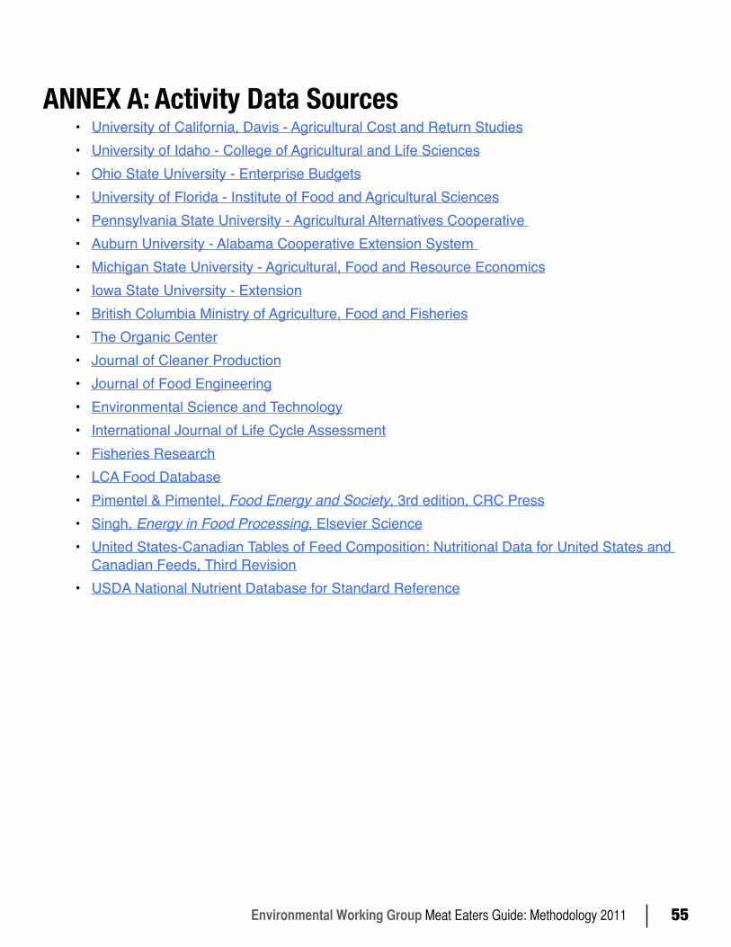
Environmental Working Group Meat Eaters Guide: Methodology 2011 55
ANNEX A: Activity Data Sources • University of California, Davis - Agricultural Cost and Return Studies• University of Idaho - College of Agricultural and Life Sciences• Ohio State University - Enterprise Budgets• University of Florida - Institute of Food and Agricultural Sciences• Pennsylvania State University - Agricultural Alternatives Cooperative • Auburn University - Alabama Cooperative Extension System • Michigan State University - Agricultural, Food and Resource Economics• Iowa State University - Extension• British Columbia Ministry of Agriculture, Food and Fisheries• The Organic Center• Journal of Cleaner Production• Journal of Food Engineering• Environmental Science and Technology• International Journal of Life Cycle Assessment• Fisheries Research• LCA Food Database• Pimentel & Pimentel, Food Energy and Society, 3rd edition, CRC Press• Singh, Energy in Food Processing, Elsevier Science• United States-Canadian Tables of Feed Composition: Nutritional Data for United States and
Canadian Feeds, Third Revision• USDA National Nutrient Database for Standard Reference
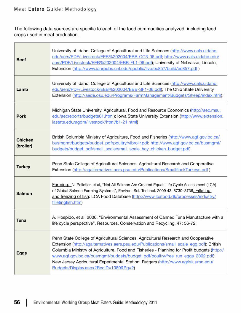
Environmental Working Group Meat Eaters Guide: Methodology 201156
M e a t E a t e r s G u i d e : M e t h o d o l o g y
The following data sources are specific to each of the food commodities analyzed, including feed crops used in meat production.
Beef
University of Idaho, College of Agricultural and Life Sciences (http://www.cals.uidaho.edu/aers/PDF/Livestock/EEB%202004/EBB-CC3-06.pdf; http://www.cals.uidaho.edu/aers/PDF/Livestock/EEB%202004/EBB-FL1-06.pdf); University of Nebraska, Lincoln, Extension (http://www.ianrpubs.unl.edu/epublic/live/ec857/build/ec857.pdf )
LambUniversity of Idaho, College of Agricultural and Life Sciences (http://www.cals.uidaho.edu/aers/PDF/Livestock/EEB%202004/EBB-SF1-06.pdf); The Ohio State University Extension (http://aede.osu.edu/Programs/FarmManagement/Budgets/Sheep/index.htm);
PorkMichigan State University, Agricultural, Food and Resource Economics (http://aec.msu.edu/aecreports/budgets01.htm ); Iowa State University Extension (http://www.extension.iastate.edu/agdm/livestock/html/b1-21.html)
Chicken (broiler)
British Columbia Ministry of Agriculture, Food and Fisheries (http://www.agf.gov.bc.ca/busmgmt/budgets/budget_pdf/poultry/vibroilr.pdf; http://www.agf.gov.bc.ca/busmgmt/budgets/budget_pdf/small_scale/small_scale_hay_chicken_budget.pdf)
Turkey Penn State College of Agricultural Sciences, Agricultural Research and Cooperative Extension (http://agalternatives.aers.psu.edu/Publications/SmallflockTurkeys.pdf )
Salmon
Farming: N. Pelletier, et al, “Not All Salmon Are Created Equal: Life Cycle Assessment (LCA) of Global Salmon Farming Systems”, Environ. Sci. Technol. 2009 43, 8730–8736; Filleting and freezing of fish: LCA Food Database (http://www.lcafood.dk/processes/industry/filletingfish.htm)
Tuna A. Hospido, et al. 2006. “Environmental Assessment of Canned Tuna Manufacture with a life cycle perspective”. Resources, Conservation and Recycling, 47: 56-72.
Eggs
Penn State College of Agricultural Sciences, Agricultural Research and Cooperative Extension (http://agalternatives.aers.psu.edu/Publications/small_scale_egg.pdf); British Columbia Ministry of Agriculture, Food and Fisheries - Planning for Profit budgets (http://www.agf.gov.bc.ca/busmgmt/budgets/budget_pdf/poultry/free_run_eggs_2002.pdf); New Jersey Agricultural Experimental Station, Rutgers (http://www.agrisk.umn.edu/Budgets/Display.aspx?RecID=1089&Pg=2)
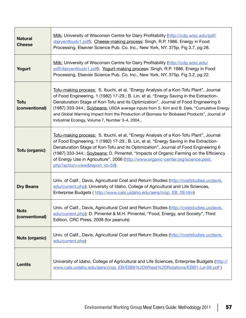
Environmental Working Group Meat Eaters Guide: Methodology 2011 57
Natural Cheese
Milk: University of Wisconsin Centre for Dairy Profitability (http://cdp.wisc.edu/pdf/dairyentbudv1.pdf); Cheese-making process: Singh, R.P. 1986. Energy in Food Processing. Elsevier Science Pub. Co. Inc., New York, NY. 375p. Fig 3.7, pg 28.
YogurtMilk: University of Wisconsin Centre for Dairy Profitability (http://cdp.wisc.edu/pdf/dairyentbudv1.pdf); Yogurt-making process: Singh, R.P. 1986. Energy in Food Processing. Elsevier Science Pub. Co. Inc., New York, NY. 375p. Fig 3.2, pg 22.
Tofu (conventional)
Tofu-making process: S. Ibuchi, et al, “Energy Analysis of a Kori-Tofu Plant”, Journal of Food Engineering, 1 (1982) 17-29.; B. Lin, et al, “Energy Saving in the Extraction-Denaturation Stage of Kori-Tofu and its Optimization”, Journal of Food Engineering 6 (1987) 333-344.; Soybeans: USDA average inputs from S. Kim and B. Dale, “Cumulative Energy and Global Warming Impact from the Production of Biomass for Biobased Products”, Journal of Industrial Ecology, Volume 7, Number 3–4, 2004..
Tofu (organic)
Tofu-making process: S. Ibuchi, et al, “Energy Analysis of a Kori-Tofu Plant”, Journal of Food Engineering, 1 (1982) 17-29.; B. Lin, et al, “Energy Saving in the Extraction-Denaturation Stage of Kori-Tofu and its Optimization”, Journal of Food Engineering 6 (1987) 333-344.; Soybeans: D. Pimentel, “Impacts of Organic Farming on the Efficiency of Energy Use in Agriculture”, 2006 (http://www.organic-center.org/science.pest.php?action=view&report_id=59).
Dry BeansUniv. of Calif., Davis, Agricultural Cost and Return Studies (http://coststudies.ucdavis.edu/current.php); University of Idaho, College of Agricultural and Life Sciences, Enterprise Budgets ( http://www.cals.uidaho.edu/aers/crop_EB_09.htm)
Nuts (conventional)
Univ. of Calif., Davis, Agricultural Cost and Return Studies (http://coststudies.ucdavis.edu/current.php); D. Pimentel & M.H. Pimentel, “Food, Energy, and Society”, Third Edition, CRC Press, 2008 (for peanuts)
Nuts (organic) Univ. of Calif., Davis, Agricultural Cost and Return Studies (http://coststudies.ucdavis.edu/current.php)
Lentils University of Idaho, College of Agricultural and Life Sciences, Enterprise Budgets (http://www.cals.uidaho.edu/aers/crop_EB/EBBI%20Wheat%20Rotations/EBB1-Le-09.pdf )
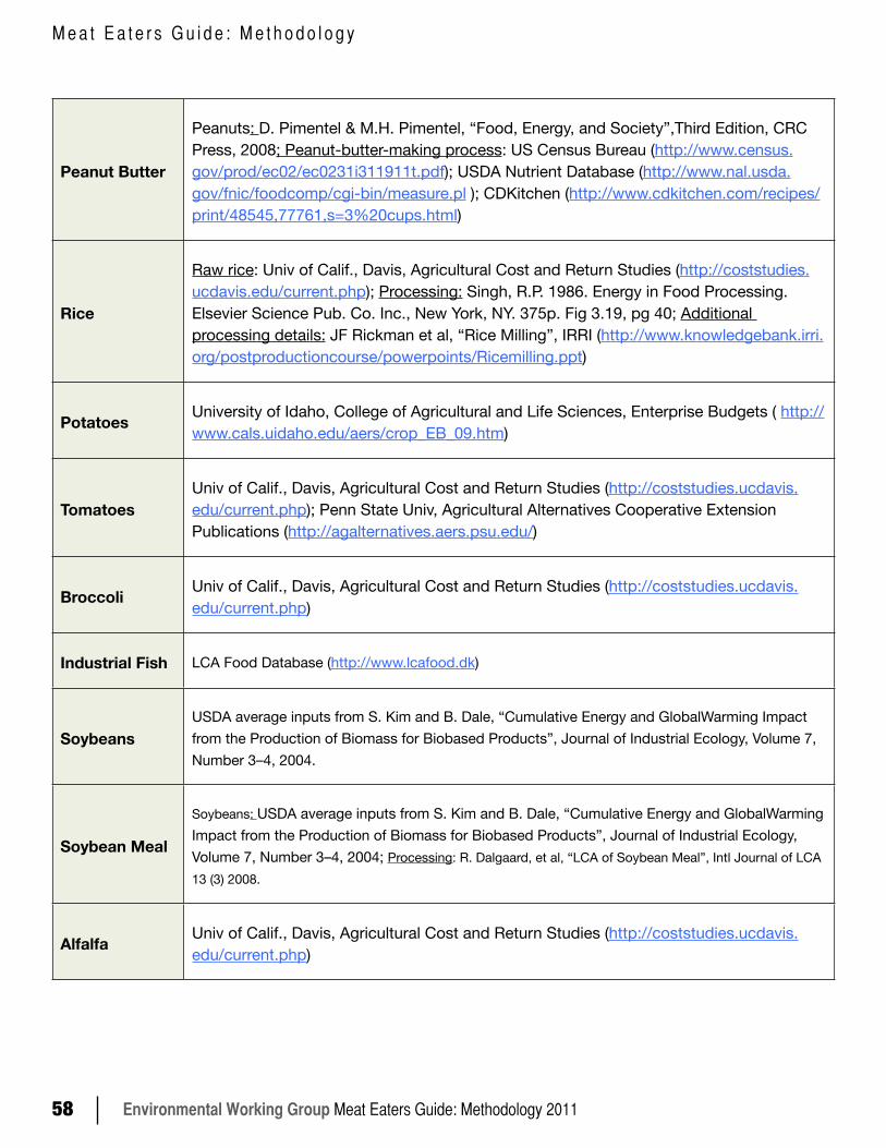
Environmental Working Group Meat Eaters Guide: Methodology 201158
M e a t E a t e r s G u i d e : M e t h o d o l o g y
Peanut Butter
Peanuts: D. Pimentel & M.H. Pimentel, “Food, Energy, and Society”,Third Edition, CRC Press, 2008; Peanut-butter-making process: US Census Bureau (http://www.census.gov/prod/ec02/ec0231i311911t.pdf); USDA Nutrient Database (http://www.nal.usda.gov/fnic/foodcomp/cgi-bin/measure.pl ); CDKitchen (http://www.cdkitchen.com/recipes/print/48545,77761,s=3%20cups.html)
Rice
Raw rice: Univ of Calif., Davis, Agricultural Cost and Return Studies (http://coststudies.ucdavis.edu/current.php); Processing: Singh, R.P. 1986. Energy in Food Processing. Elsevier Science Pub. Co. Inc., New York, NY. 375p. Fig 3.19, pg 40; Additional processing details: JF Rickman et al, “Rice Milling”, IRRI (http://www.knowledgebank.irri.org/postproductioncourse/powerpoints/Ricemilling.ppt)
Potatoes University of Idaho, College of Agricultural and Life Sciences, Enterprise Budgets ( http://www.cals.uidaho.edu/aers/crop_EB_09.htm)
TomatoesUniv of Calif., Davis, Agricultural Cost and Return Studies (http://coststudies.ucdavis.edu/current.php); Penn State Univ, Agricultural Alternatives Cooperative Extension Publications (http://agalternatives.aers.psu.edu/)
Broccoli Univ of Calif., Davis, Agricultural Cost and Return Studies (http://coststudies.ucdavis.edu/current.php)
Industrial Fish LCA Food Database (http://www.lcafood.dk)
SoybeansUSDA average inputs from S. Kim and B. Dale, “Cumulative Energy and GlobalWarming Impact from the Production of Biomass for Biobased Products”, Journal of Industrial Ecology, Volume 7, Number 3–4, 2004.
Soybean Meal
Soybeans: USDA average inputs from S. Kim and B. Dale, “Cumulative Energy and GlobalWarming Impact from the Production of Biomass for Biobased Products”, Journal of Industrial Ecology, Volume 7, Number 3–4, 2004; Processing: R. Dalgaard, et al, “LCA of Soybean Meal”, Intl Journal of LCA 13 (3) 2008.
Alfalfa Univ of Calif., Davis, Agricultural Cost and Return Studies (http://coststudies.ucdavis.edu/current.php)

Environmental Working Group Meat Eaters Guide: Methodology 2011 59
Annex B Assumptions for Cooking times and Methods
Product Cook-ing Appliance
Tem-pera-ture
Pre-heating time
Cooking Time/ lb product
Cooking Time/kg product
Source
Lamb oven 325°F 10 min 30 min/ lb 30 min/ .45kg
http://www.hoptechno.com/booklamb.htm
Beef stove top medium-high heat 10 min/ .3125
10 min/ 0.1417 kg
http://www.thejoykitch-en.com/recipe
Pork Oven 350°F 10 min 30 min/1 lb 30 min/ .45kg
http://www.fsis.usda.gov/Fact_Sheets/Pork_From_Farm_to_Table/index.asp
Chicken oven 350°F 10 min 1.5hrs/4lbs 1.5 hrs/1.814
http://www.fsis.usda.gov/factsheets/Chick-en_Food_Safety_Fo-cus/index.asp
Turkey oven 325°F 10 min 3.25hours/ 8 lbs
3.25 hrs/3.6287
http://www.fsis.usda.gov/Fact_Sheets/Lets_Talk_Turkey/index.asp
Salmon oven 350°F 10 min 30 min/5 lbs
30 min/2.26 kg
http://www.reci-petips.com/kitchen-tips/t--1231/fish-cook-ing-guide.asp
Tofu stove top medium to high heat 8 min 8 min/ .45kg http://www.eatingwell.com/recipes/spice_crusted_tofu.html
Orchardgrass Univ of Calif., Davis, Agricultural Cost and Return Studies (http://coststudies.ucdavis.edu/current.php)
CornNASS data from N. Pelletier, et al, “Comparative life cycle environmental impacts of three beef production strategies in the Upper Midwestern United States”, Agricultural Systems 103, 2010.
Corn SilageNASS data from N. Pelletier, et al, “Comparative life cycle environmental impacts of three beef production strategies in the Upper Midwestern United States”, Agricultural Systems 103, 2010.
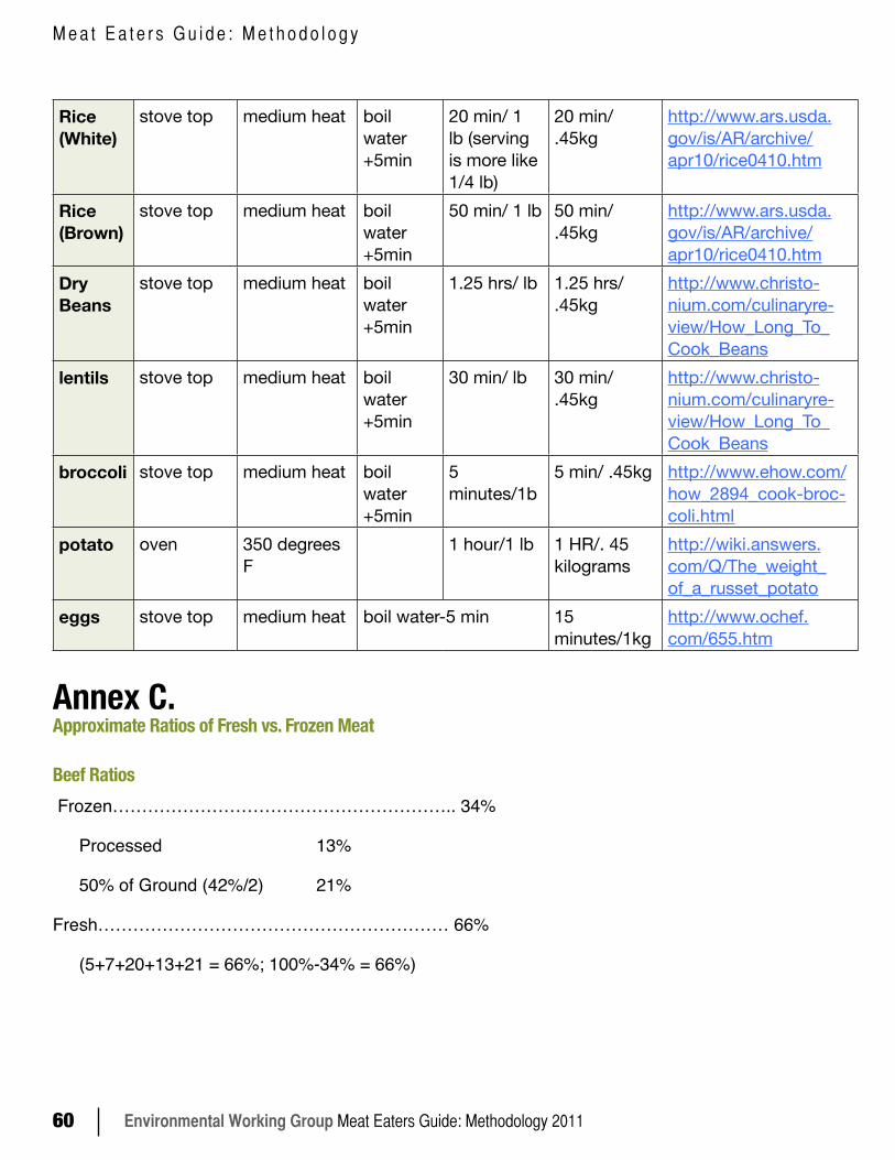
Environmental Working Group Meat Eaters Guide: Methodology 201160
M e a t E a t e r s G u i d e : M e t h o d o l o g y
Rice (White)
stove top medium heat boil water +5min
20 min/ 1 lb (serving is more like 1/4 lb)
20 min/ .45kg
http://www.ars.usda.gov/is/AR/archive/apr10/rice0410.htm
Rice (Brown)
stove top medium heat boil water +5min
50 min/ 1 lb 50 min/ .45kg
http://www.ars.usda.gov/is/AR/archive/apr10/rice0410.htm
Dry Beans
stove top medium heat boil water +5min
1.25 hrs/ lb 1.25 hrs/ .45kg
http://www.christo-nium.com/culinaryre-view/How_Long_To_Cook_Beans
lentils stove top medium heat boil water +5min
30 min/ lb 30 min/ .45kg
http://www.christo-nium.com/culinaryre-view/How_Long_To_Cook_Beans
broccoli stove top medium heat boil water +5min
5 minutes/1b
5 min/ .45kg http://www.ehow.com/how_2894_cook-broc-coli.html
potato oven 350 degrees F
1 hour/1 lb 1 HR/. 45 kilograms
http://wiki.answers.com/Q/The_weight_of_a_russet_potato
eggs stove top medium heat boil water-5 min 15 minutes/1kg
http://www.ochef.com/655.htm
Annex C. Approximate Ratios of Fresh vs. Frozen Meat
Beef Ratios Frozen………………………………………………….. 34%
Processed 13%
50% of Ground (42%/2) 21%
Fresh…………………………………………………… 66%
(5+7+20+13+21 = 66%; 100%-34% = 66%)
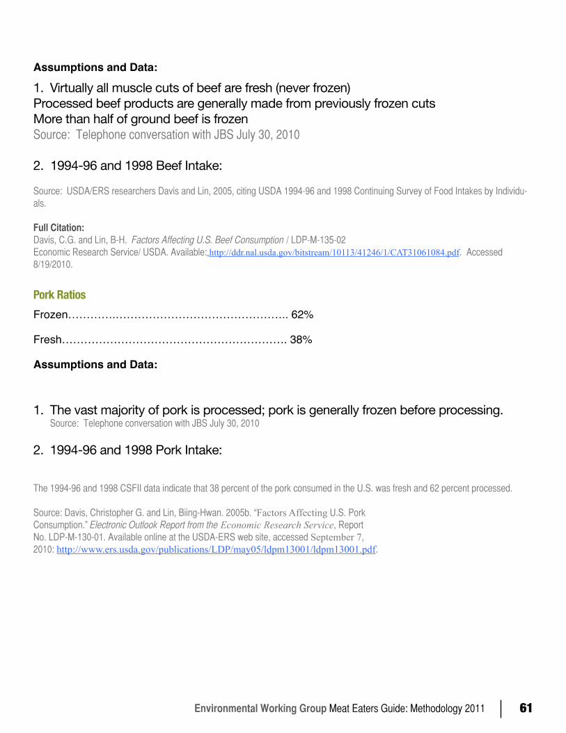
Environmental Working Group Meat Eaters Guide: Methodology 2011 61
Assumptions and Data:
1. Virtually all muscle cuts of beef are fresh (never frozen)Processed beef products are generally made from previously frozen cutsMore than half of ground beef is frozenSource: Telephone conversation with JBS July 30, 2010
2. 1994-96 and 1998 Beef Intake:
Source: USDA/ERS researchers Davis and Lin, 2005, citing USDA 1994-96 and 1998 Continuing Survey of Food Intakes by Individu-als .
Full Citation:Davis, C .G . and Lin, B-H . Factors Affecting U.S. Beef Consumption / LDP-M-135-02Economic Research Service/ USDA . Available: http://ddr.nal.usda.gov/bitstream/10113/41246/1/CAT31061084.pdf . Accessed 8/19/2010 .
Pork RatiosFrozen………….……………………………………….. 62%
Fresh……………………………………………………. 38%
Assumptions and Data:
1. The vast majority of pork is processed; pork is generally frozen before processing. Source: Telephone conversation with JBS July 30, 2010
2. 1994-96 and 1998 Pork Intake:
The 1994-96 and 1998 CSFII data indicate that 38 percent of the pork consumed in the U .S . was fresh and 62 percent processed . Source: Davis, Christopher G . and Lin, Biing-Hwan . 2005b . “Factors Affecting U .S . PorkConsumption .” Electronic Outlook Report from the Economic Research Service, ReportNo . LDP-M-130-01 . Available online at the USDA-ERS web site, accessed September 7,2010: http://www.ers.usda.gov/publications/LDP/may05/ldpm13001/ldpm13001.pdf .

Environmental Working Group Meat Eaters Guide: Methodology 201162
M e a t E a t e r s G u i d e : M e t h o d o l o g y
Assumptions and Data:
1. Virtually all muscle cuts of beef are fresh (never frozen)Processed beef products are generally made from previously frozen cutsMore than half of ground beef is frozenSource: Telephone conversation with JBS July 30, 2010
2. 1994-96 and 1998 Beef Intake:
Source: USDA/ERS researchers Davis and Lin, 2005, citing USDA 1994-96 and 1998 Continuing Survey of Food Intakes by Individu-als .
Full Citation:Davis, C .G . and Lin, B-H . Factors Affecting U.S. Beef Consumption / LDP-M-135-02Economic Research Service/ USDA . Available: http://ddr.nal.usda.gov/bitstream/10113/41246/1/CAT31061084.pdf . Accessed 8/19/2010 .
Pork RatiosFrozen………….……………………………………….. 62%
Fresh……………………………………………………. 38%
Assumptions and Data:
1. The vast majority of pork is processed; pork is generally frozen before processing. Source: Telephone conversation with JBS July 30, 2010
2. 1994-96 and 1998 Pork Intake:
The 1994-96 and 1998 CSFII data indicate that 38 percent of the pork consumed in the U .S . was fresh and 62 percent processed . Source: Davis, Christopher G . and Lin, Biing-Hwan . 2005b . “Factors Affecting U .S . PorkConsumption .” Electronic Outlook Report from the Economic Research Service, ReportNo . LDP-M-130-01 . Available online at the USDA-ERS web site, accessed September 7,2010: http://www.ers.usda.gov/publications/LDP/may05/ldpm13001/ldpm13001.pdf .
Chicken RatiosFresh………….……………………………………….. 60%
Frozen………….……………………………………… 40%Source: Telephone conversation with National Chicken Council August 12, 2010
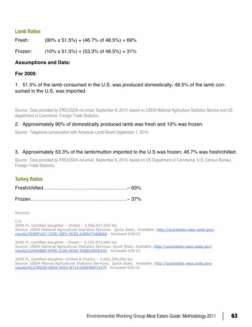
Environmental Working Group Meat Eaters Guide: Methodology 2011 63
Lamb RatiosFresh: (90% x 51.5%) + (46.7% of 48.5%) = 69%
Frozen: (10% x 51.5%) + (53.3% of 48.5%) = 31%
Assumptions and Data:
For 2009:
1. 51.5% of the lamb consumed in the U.S. was produced domestically; 48.5% of the lamb con-sumed in the U.S. was imported.
Source: Data provided by ERS/USDA via email, September 8, 2010, based on USDA National Agriculture Statistics Service and US department of Commerce, Foreign Trade Statistics .
2. Approximately 90% of domestically produced lamb was fresh and 10% was frozen.Source: Telephone conversation with American Lamb Board September 1, 2010 .
3. Approximately 53.3% of the lamb/mutton imported to the U.S was frozen; 46.7% was fresh/chilled.Source: Data provided by ERS/USDA via email, September 8, 2010, based on US Department of Commerce, U .S . Census Bureau, Foreign Trade Statistics .
Turkey RatiosFresh/chilled……………………………………………– 63%
Frozen…………………………………………………..– 37% Sources:
U.S.2009 FI, Certified slaughter – chilled – 3,556,427,000 lbs.Source: USDA National Agricultural Statistics Services. Quick Stats. Available: http://quickstats.nass.usda.gov/results/5D85F1A7-253E-39F2-9C83-A395A74686A8. Accessed 9/8/10.
2009 FI, Certified slaughter – frozen – 2,105,972,000 lbs.Source: USDA National Agricultural Statistics Services. Quick Stats. Available: http://quickstats.nass.usda.gov/results/0240AB6E-6F98-3100-9D00-EA881E83E420. Accessed 9/8/10.
2009 FI, Certified slaughter (chilled & frozen) – 5,662,399,000 lbs.Source: USDA Ntional Agricultural Statistics Services. Quick Stats. Available: http://quickstats.nass.usda.gov/results/6127ED36-0659-34D2-871A-656F86FC447F. Accessed 9/8/10.