Life Tables with Covariates: Dynamic Model for Nonlinear Analysis of Longitudinal Data

Life Tables with Covariates: Dynamic Model forNonlinear Analysis of Longitudinal Data

I. AkushevichA. KulminskiK. G. MantonCenter for Demographic Studies, Duke University, Durham,North Carolina, USA

Life table models based on nonlinear dynamics of risk factors are developed usingstochastic differential equations for individual changes and on the resultingFokker-Planck equation to describe population changes. Central to the model isa microsimulation strategy developed as a numerical procedure to represent amortality effect when analytic approaches are not applicable. The model is appliedto the Framingham Heart Study 46-year follow-up data. Life table functions andprojections of risk factors are calculated to demonstrate the nonlinear effects onobservable quantities over time. A set of statistically significant nonlinear contri-butions to covariate dynamics is identified. Their synergistic effect on dynamicsand use of them as ‘‘new’’ risk factors are discussed. An important advantage ofthis approach is the ability to study the effects of health interventions at theindividual level. This is illustrated in several examples.

Keywords: stochastic differential equations; quadratic hazard; life table; risk factors;Fokker-Planck equation; longitudinal data

INTRODUCTION

Despite numerous experimental and theoretical attempts to under-stand the forces shaping the human mortality curve at late ages, manymethodological problems remain to be solved before a model can bedeveloped that accurately reflects changes in the complex biology of

This research was supported by grant P01 AG17937-05 from the National Institutesof Health=National Institute on Aging. The Framingham Heart Study (FHS) is conduc-ted and supported by the NHLBI in collaboration with the FHS Study Investigators.This paper was prepared using a limited access dataset obtained by the NHLBI and doesnot necessarily reflect the opinions or views of the FHS Study or the NHLBI.

Address correspondence to Igor Akushevich, Ph.D., Center for Demographic Studies,Duke University, 2117 Campus Drive, Box 90408, Durham, NC 27708-0408, USA.Tel.: 919-668-2715, E-mail: [email protected]

Mathematical Population Studies, 12:51–80, 2005

Copyright # Taylor & Francis Inc.

ISSN: 0889-8480 print=1543-5253 online

DOI: 10.1080/08898480590932296

51

individuals (Manton and Yashin, 2000). Theoretical insights intohuman failure processes also have the difficulty of reacting to therapid production of findings from experimental, clinical and popu-lation studies. Explanations based on concepts of heterogeneity inmortality, individual adaptation, hormesis or on the general proper-ties of complex multistage dynamic systems sometimes appear to con-tradict each other (Manton, 1999; Michalski et al., 2003; Stebbing,1987 and Vaupel and Yashin, 1985) and existing demographic models.Using only population survival data restricts analysis to mortality(time to failure) models, so contradictions may not even be observed(Manton and Stallard, 1988). A frequently used model, the Gompertzhazard, does not fit mortality in human populations at later ages(Lew and Garfinkel, 1984, 1987; Carey et al., 1992). Models thatassume characteristics of aging are specific to individuals have thedifficulty of interpreting the distribution of these characteristics inpopulation (heterogeneity) as biologically meaningful (e.g., the use ofa gamma or inverse Gaussian mixed Gompertz (Dubey, 1967, Mantonet al., 1986)). Standard longitudinal analyses employ the Coxregression with proportional risk assumptions which can be difficultto motivate biologically (Woodbury et al., 1981).

The problems in constructing bio-demographic models of mortalityare enhanced by the complex nature of longitudinal studies. Usually,time series formed by repeated measurements in longitudinal studiesare insufficiently lengthy or detailed. This prevents the developmentof modeling techniques suitable for comprehensively describing a sam-ple of three dimensional (3D) measurements formed by persons, mea-sures, and time. Moreover, the individual time series are randomlyended because of different types of failure events. Recent long-termstudies (Framingham Heart Study, National Long Term Care Survey)can be used as the basis for longitudinal bio-demographic modeling.

Thus, further development of biologically motivated populationmodels—as well as the extension of existing bio-demographic modelsfor analyzing longitudinal physiological change and survival data—are needed. One biologically detailed model suitable for describing a‘‘long’’ time series of longitudinal data (typically less than fifty mea-surements over time) is based on a high dimensional random walkfor individuals, producing a Fokker-Planck equation for the popu-lation (Woodbury and Manton, 1977). This model is based on a biologi-cally motivated assumption of a quadratic hazard that exploits themathematical formalism of stochastic differential equations. Thequadratic hazard is justified by J or U-shaped forms of hazards as afunction of risk factors observed in many epidemiological studies(Witteman et al., 1994). A comprehensive review of the stages of

52 I. Akushevich et al.

development of demographic models, from conventional models toquadratic hazard, is given by Yashin et al. (2000). Such models are dis-tinct from conventional time series models, which deal with long timeseries data (typically more than fifty measurements over time) collectedfor one subject (e.g., for one individual), i.e., they are 2D models whilelongitudinal studies require techniques dealing with the 3D sample.

In our approach it is assumed that the evolution of the individual’sstate and survival probability SðxÞ can be described by a system ofstochastic differential equations for stopped processes. The failureprobability is modeled as a positive definite quadratic form. The mini-mum corresponds to a point (or a domain) in the covariate state spaceoptimal to health status. The probability of death increases far fromthis optimal region. This model generalizes the concepts of frailtyand competing risks, and, in addition, allows one to consider thedynamics of observed and unobserved covariates (risk factors). Withthis model it is possible to calculate life table functions and to forecastthe characteristics of the health state distribution over age and time(Woodbury and Manton, 1983; Manton et al., 1992). However, usingonly linear state dynamic equations restricts the accuracy andpredictive power of the model.

We generalize this model to include the effects of nonlinear interac-tions among the risk factors. There are several reasons to constructnonlinear generalizations. First, statistical analysis of experimentalmedical data shows that many more parameters can be introducedinto dynamic models to achieve an adequate description of the data(Kulminski et al., 2004). Second, the solution of the system for lineardynamics, the Gaussian random process, is not sufficiently rich.Experimental covariate distributions are described by Gaussian lawonly as a rough approximation, and such facts as the existence of anonzero probability of having negative values of covariates are alsoinappropriate consequence of the assumption. Third, since a humanbeing is a complex biological system, it is reasonable to expect thatnonlinear interactions among risk factors (covariates) describinghealth status can be significant. The price of not using the restrictiveassumptions necessary for linear model construction is that analyticformulas for projections may not work. Consequently, we developnew techniques based on microsimulation of individual trajectoriesin state space for linking nonlinear models with mortality. Thus, anew population model for covariate dynamics and covariate dependentfailure events is constructed. The parameters of the model are esti-mated from data collected in the Framingham Heart Study throughmaximum likelihood. We performed numerical analyses wherethe impact of linear and nonlinear effects on covariate dynamics and

Life Tables with Covariates 53

survival is studied. An important part of our analysis is the search foressential nonlinear contributions to covariate dynamics and investi-gation of their synergistic effects. Finally, we show how to includeeffects of non-Gaussian diffusion effects and how to study healthstatus interventions.

DYNAMIC MODELING TECHNIQUE

Comprehensive longitudinal analysis requires advanced techniques tofully utilize the rich potential of longitudinal data that link dynamicsand random failure events (death, disease). Such techniques should bebiologically motivated. The basis of such a methodology was developedby Woodbury and Manton (1977). Since it is not a standard tool weprovide a detailed derivation of the basic linear model to make cleanits logic, assumptions, and restrictions. Then we extend this modelto include the effects of nonlinear interaction among risk factors.

Assume that the health state of an organism can be described byJ physiological variables (or risk factors). The number of risk factorsis not limited and can be as many as necessary (or available) to com-pletely describe the individual’s health state. These variables constitutea state space in which each point represents an individual at time t. Lifeof an individual is approximated by a trajectory in the state space, withbeginning and end corresponding to birth and death. The set of allpoints at a fixed instant of time represents a population as a whole.All population characteristics are calculated as means over individuals.

Two important points to be addressed are i) the laws governing indi-vidual dynamics (i.e., the laws responsible for changing covariateswith time), and ii) time and causality of failure events. Usually, evol-ution of objects in a state space is described by a system of ordinarydifferential equations. A well-known example is a system of Newtonequations governing movement of particles in statistical systems.When the state space is associated with the individual’s health state,the construction of an exact system of master equations for describinghealth trajectories is not helpful for two reasons. First, an organism isvery complicated and a finite number of risk factors can only approxi-mate its state. Second, the environment can influence the health state.Although the dynamics of risk factors can be modeled deterministi-cally, a natural way to describe the environment contribution, as wellas the latent (unobserved) risk factors, is by stochastic components.Thus, to model covariate dynamics we use a system of stochasticdifferential equations, i.e.,

dxt ¼ uðxt; tÞdtþ rðxt; tÞdWt: ð1Þ


Equation (1) represents the changes for organism i on each of J covari-ates x ¼ ðxj; j ¼ 1; 2; . . . ;JÞ or risk factors at time t. The total move-ment dxt of individual i during time dt in the state space is the sumof deterministic changes uðxi; tÞdt and the random walk, rðxt; tÞdWt.Wt is a standard Wiener process.

Dynamic Eq. (1) for state variables has to be completed by an equa-tion describing random stopping (killing or absorption). This can bedone in terms of function describing the probability of survival. Thenchanges in the conditional survival function Sðtjxt0 ; . . . ;xtÞ in time are

dSðtjxt0 ; . . . ;xtÞ ¼ �lðxt; tÞSðtjxt0 ; . . . ;xtÞdt: ð2Þ

Sðtjxt0 ; . . . ;xtÞ is the probability of surviving for individual i with statespace trajectory xt0 ; . . . ;xt. The change of the survival probabilitySðtjxt0 ; . . . ;xtÞ is proportional to mortality lðxt; tÞ. Necessary and suf-ficient conditions justifying (2) are given in Yashin and Arjas (1988).

The system of stochastic differential equations (1) and (2) is writtenin Ito form. Equation (1) governs movements of individuals over thestate space. It can be interpreted as the development of a cohort in timeunder a deterministic law with stochastic deviations of individual trajec-tories. Individual trajectories are randomly stopped. The distribution ofthe stopping moments is described by Eq. (2). In terms of the theory ofdifferential equations, the system of Eq. (1) and (2) represents astochastic Cauchy problem generalized to random stopping. The stoch-astic process defined by system (1) and (2) is Markovian. Although thissomewhat restricts the model, the importance of this restriction is oftenoverestimated. In fact, it is difficult to argue against a point of view thatthe whole history of a person is hidden within the present state, ifthe state space has sufficiently high dimensions (e.g., history, recentdynamics or memory effects can be modeled by adding covariate deriva-tives up to necessary orders as independent variables). The practicaluse of dozens of covariates as a state space is only an approximationdictated by experimental data, but it is not the principle restriction ofthe model. Besides, using Markovian processes allow the use of well-developed mathematical formalism based on the Ito formula, theKolmogorov-Fokker-Planck equation and the Feynman-Kac formula.

The system of equations (1) and (2) has to be completed by the initialconditions for the distribution of covariates with probability densityp1ðt0Þ at initial time t0 (i.e., when a cohort was established). Then theCauchy problem can be solved analytically or numerically. Currently,the theory of the numerical solution of such problems is under intensedevelopment. The general approach for constructing a solution is to usea stochastic generalization of the schemes of numerical solutions forordinary differential equations (e.g., Euler, Runge-Kutta). This


approach is based on discretization of time interval, and it uses theTaylor-Ito expansion of the Ito stochastic processes. The numericalschemes differ only by the order of the approximation of the stochasticintegrals. Meanwhile, for stopped processes the theory is not so welldeveloped. Thus, to construct a solution we can use discretization,which is well suited both for analytical and for numerical solutions.The simplest discrete solution can be constructed using Euler’s scheme,which is transparent and has a natural algorithm, which can be con-veniently generalized to stopped processes, i.e.,

xtþ1 ¼ x�t þ �uuðx�

t ; tÞ þ �rrðx�t ; tÞDWt; ð3Þ

with the correction that is provided by mortality. The superindex � indi-cates that x�

t is conditional on survival in the next discrete time inter-val. The discrete form of the solution is chosen because of thestructure of data to be used for parameter estimation and because ofour desire to develop a model for cumulative, rather then differential,mortality. This allows us to avoid difficulties in defining risk factorsat the moment of death. Because of dependence of the matrix �rrðxt; tÞonxt, it is necessary to distinguish between the Ito and the Stratonovichdefinitions. We define the model using Ito’s definition because it corre-sponds to general demographic definitions (e.g., survival in one year forindividuals having a certain age at the beginning of the interval).

We focus on a class of nonlinear models in which deterministic driftuðxi; tÞ is a nonlinear function of the risk factors.

It can be shown that if all elements of a drift vector udðxt; tÞ

udj ðxt; tÞ ¼ ujðxt; tÞ þ

1

2

Xj1j2

@rjj2ðxt; tÞ@xj1

rj1j2ðxt; tÞ ð4Þ

are differentiable and all elements of a diffusion matrix

rdðxt; tÞ ¼ rðxt; tÞrTðxt; tÞ

are twice differentiable, then the transferring probability density ofthe Markovian process pðxt; tjys; sÞ between states xt and yt ðt � sÞobeys the generalized Fokker-Planck equation or second Kolmogorovequation (Risken, 1996):

@pðxt; tjys; sÞ@t

¼ �Xj

@

@xjudj ðxt; tÞpðxt; tjys; sÞ

h i

þ 1

2

Xj1j2

@2

@xj1xj2rj1j2ðxt; tÞpðxt; tjys; sÞ� �

� lðxt; tÞpðxt; tjys; sÞ; ð5Þ


with initial condition

limt#s

pðxt; tjys; sÞ ¼ dðxt � ytÞ:

An analytic solution of the stochastic Cauchy problem formulated inthe form of the Fokker-Planck equation can be found under specificconditions (Woodbury and Manton, 1977). First is that the populationdistribution can be described at time t as a multivariate normal distri-bution Nðlt; nt;VtÞ whose three parameters represent the populationsize (lt), the vector of physiological variable means (nt ¼ EðxtÞ), andthe variance-covariance matrix (Vt ¼ VarðxtÞ). This is equivalent toassuming a linear drift over xt and constant diffusion. The lastterm in (5) (lp), corresponding to the force of mortality, changes thenormalization (lt) of the multivariate distribution function over time.

The second assumption is that mortality is a quadratic function ofrisk factors,

lðxtÞ ¼ l0 þ btxt þ1

2xTt Btxt: ð6Þ

This function describes the probability of dying conditional on thehealth state described by risk factors xt. The quadratic form of lt helpsto model a situation when there is a point (or a domain) in the statespace optimal for health (e.g., the vertex of paraboloid), and mortalityincreases going away from this domain. Hence, matrix Bt is assumedto be positive definite. For discrete time l0, bt and Bt have the meaningof coefficients of the cumulative force of mortality for the age intervalðt; tþ 1Þ. The numerical estimation of these parameters is discussed inthe Section ‘‘Data Analysis.’’

The first and second assumptions are sufficient to show that thecovariate distribution of survivors over the time period is normalðNðl�t ; n�t ;V�

t ÞÞ. This allows us to calculate the characteristics of the sur-viving population (variables with asterisk) in terms of the characteris-tics of the total population and the hazard coefficients (Woodbury andManton, 1983)

n�t ¼ nt � V�t ðbt þ BtntÞ; V�

t ¼ ðV�1t þ BtÞ�1: ð7Þ

Another consequence is an explicit expression for the normalizationparameter l�t ¼ ltþ1 of the risk factor distribution related to the sur-vival function lt=l0 ¼ St

def¼¼ EðSðtjxt0 ; . . . ;xtÞÞ. The survival function

starting as St0 ¼ 1 is,

Stþ1 ¼ StjI þ VtBtj�1=2 explðntÞ þ lðn�t Þ

2� 2l

nt þ n�t2

� �� : ð8Þ


Formula (8) is obtained without additional assumptions about theform of the dynamic equations. The time period appearing in l.h.s. of(8) exactly corresponds to the time period of the cumulative force ofmortality in r.h.s.

Next we construct a dynamic model describing the changes in riskfactors over time. We discuss below different models, keeping in mindthe parameter estimation for covariates measured at discrete times.The simplest model used by Woodbury and Manton (1977) is linearwith respect to variables x�

t ,

xtþ1 ¼ u0 þ Rx�t þ E: ð9Þ

We use Gaussian assumptions about the initial covariate distributionwith probability density pGðxt0 ; nt0 ;Vt0Þ, where mean nt0 and variance-covariance matrix Vt0 are estimated from data. The vector u0 andthe regression matrix R are calculated using ordinary least squaremethods (see Section ‘‘Data Analysis’’), and E ¼ rðx; tÞdWt will beapproximated by a time-independent normally distributed randomvariable. The asterisk for x in the R.H.S. of Eq. (9) emphasizes thefact that x� belongs to the distribution of individuals who are aliveat time ðtþ 1Þ. A valuable feature of the linear model is that itpreserves the normality of covariate distribution over time. Thevector of means and the variance-covariance matrix can be calculatedas:

ntþ1 ¼ u0 þ Rn�t ; Vtþ1 ¼ RþRV�t R

T; ð10Þ

where R ¼ VarðEÞ is the empirical diffusion matrix. Thus, this model isbased on the assumption that changes in each risk factor are related tothe linear superposition on their prior values.

Assumptions about linear drift and constant diffusion restrict thepredictive power of the model. The basic restriction is due to the nor-mal form of the covariate distribution which is only a first approxi-mation. Apart from the strict analytical form for this distribution, itimplies the finite probability of having unnatural (negative) valuesfor covariates. Attempts to overcome this obstacle (e.g., to artificiallykeep covariates positive) require functional dependence of diffusionon covariates that destroy the normality of the covariate distribution.Another problem is related to assumptions about linear drift. Autore-gression models used to estimate covariate dynamics have J para-meters per covariate (J ¼ 11 in our case), while longitudinal surveysprovide about I �N measurements per covariate. Thus, the linearmodel may not be sufficiently rich to describe such data. Third, theanalytical solution provides projections for population characteristics


at the (macro) population level with limited possibilities for modelingat the individual level. These concerns require generalizing the model.

Recently, attention has been devoted to extensions of the linearmethods of data analysis to consider nonlinear dynamics and memoryeffects (Pe~nna et al., 2001). Nonlinear time series analysis deals withthe ‘‘degree of nonlinearity,’’ i.e., how strongly nonlinear the systemis. The importance of the system’s prehistory can be characterizedby ‘‘degree of memory.’’ Implementing such effects into our longitudi-nal model, the following equation can be written:

xtþ1 ¼ u0 þ Fðxt; . . . ;xt�m; aÞ þ E; ð11Þ

where m is the depth of the memory, a is a vector of parameters andFð�Þ is a nonlinear function of covariates and, perhaps, of parameters.

To simplify the problem one can consider two limits of the modelwith either memory or nonlinear effect. For the memory effect themodel is,

xtþ1 ¼ u0 þ Rx�t þ Tx��

t�1 þ � � � þ E: ð12Þ

The double asterisk means survival over two time periods. Analysis ofthe 46-year follow-up Framingham data shows that there are suf-ficient data to estimate several terms in Eq. (12). This model alsopropagates a normal distribution. The simplest case with m ¼ 1 in(12) and with no correlations between x�

t and x��t�1 is considered by

Akushevich et al. (2003). In longitudinal studies in which time seriesare relatively short, using (12) sacrifices the initial waves.

In the second limit the model includes only nonlinearities. The sim-plest nonlinear model assumes, in addition to describing the effect oflinear superposition of all risk factors on future health, that each riskfactor can ‘‘interfere’’ with the others, inducing additional changes.The interference of two (or more) variables can be represented by theirscalar product as:

xtþ1;j ¼ u0;j þXk

Rjkx�t;k þ

Xk;l

Cjklx�t;kx

�t;l þ � � � þ Ej: ð13Þ

We deal with model (13) with only second order nonlinearities. By esti-mating the coefficients in vector u0 and matrices R and C, we can use(13) to study the synergistic effect in the dynamics of risk factors andin health changes.

Since the nonlinear model does not propagate a Gaussian distri-bution over time, exact analytical formulas like (10) cannot beobtained. What can be obtained analytically are formulas for the meanand variance-covariance matrix if the multidimensional covariate


distribution is approximated by a normal distribution at each timeinterval. These equations read:

ntþ1;j ¼ u0;j þXk

Rjkn�k þXk;l

CjklðV�kl þ n�kn

�l Þ ð14Þ

and

Vtþ1;ij ¼ Rij þXkl

RikV�klRjl þ 2

Xmkl

RimCjklðn�l V�mk þ n�kV

�ml � 2n�l n

�kn

�mÞ

þXmnkl

CimnCjklðV�mkV

�nl þ V�

mlV�nk � n�l n

�kn

�mn

�nÞ: ð15Þ

For simplicity, we dropped index t at quantities with asterisk in r.h.s.:n�t;k � n�k and V�

t;mk � V�mk. These formulas complete the standard sys-

tem of difference equations (in addition to Eq. (7) and (8)). Hence,the approximate analytical calculation of life tables can be developedfor the nonlinear case, but it will be not exact. Moreover, the accuracyof this approximation is difficult to control.

An exact procedure of propagation based on nonlinear formulasincluding mortality effects can be developed using microsimulation.In this approach random stopped individual trajectories are simulatedas a solution (3) of the system of stochastic differential equations.Instead of analytical formulas, the results for all quantities of interestare calculated as expectations over all simulated trajectories. Thisapproach can be applied for the linear model. A comparison of cal-culated expectations with analytical projections provide a check offormulas and numerical codes.

MICROSIMULATION AND MORTALITY EFFECTS

The microsimulation procedure is based on methods for simulating thetrajectories for each person in the cohort. The mathematical basis ofthis technique is the theory of stochastic processes and the simulationmethods of solving stochastic differential equations (Kloeden, Platen,1992; Kloeden et al., 1994; Wolf, 2001 on applications of micro-simulation in the social sciences). The individual trajectory is con-structed as a solution of a deterministic system of differentialequations which is obtained after specific realizations of randomvariables: the Wiener process in (1), the initial values of covariates,and random stopping.

To begin, a cohort of individuals at an initial time t0 is constructed.Cohort size is limited only by the required statistical accuracy. Theinitial values of covariates for all individuals in the cohort are simulated


assuming a multidimensional Gaussian distribution. Means nt0 and thecoefficients of the variance-covariance matrix Vt0 can be estimated fromdata at the initial age or can be based onmodel assumptions. Individualcovariates xt0 are simulated using a theorem about the decomposition ofthe multivariate normally distributed random vector:

xt0 ¼ nt0 þDTZ ð16Þwhere Z is a vector of standardized normally distributed numbersZi � Nð0; 1Þ and matrix D is the square root of the matrixVt0 ðVt0 ¼ DTDÞ.

Generally, the assumption of a normal distribution is not necessary.Non-Gaussian corrections can be added to study the non-Gaussianeffects of the initial population distribution on projections. Age atthe initial time is fixed in calculations. Generalizations to the variableinitial age are straightforward. For fixed age, the variance-covariancematrices (Vt and R) have to be calculated conditional on age.

Having the initial distribution of individuals, we then model tra-jectories in the J dimensional state space in two steps. First, theprobability SðtjxtÞ ¼ Ext0

;...;xt�1ðSðtjxt0 ; . . . ;xtÞÞ of survival for each

individual is calculated using the mortality rate lt for the interval(t; tþ 1):

SðtjxtÞ ¼ expð�ltÞ ¼ exp �l0 � btxt �1

2xTt Btxt

� �: ð17Þ

The integral over the time period (t; tþ 1) does not appear explicitlybecause it is hidden in coefficients l0, bt and Bt, which are estimatedas integrated (cumulative) characteristics. Each individual in thecohort is simulated to survive, or not, in accordance with probabilitySðtjxtÞ. To do this, a uniformly distributed random number r is gener-ated. If r > SðtjxtÞ, the individual is assumed to have died and isremoved from the cohort. It is possible to demonstrate that the pro-cedure of random removal of individuals from the cohort with nor-mally distributed covariates xt gives a survival population which isalso normally distributed, and that relations between parameters ofthese two distributions are given by (7). In fact, the simulated numberof survivors having risk factors in the neighborhood of xt, i.e., in(xt � 1

2Dxt, xt þ 12Dxt), is ltSðtjxtÞpGðxt; nt;VtÞDxt. In the limit of large

cohort size this number should exactly coincide with the number ofindividuals in the state space domain for survival distributionl�t pGðxt; n�t ;V

�t ÞDxt. This means that the following equality has to be

valid for any xt:

l�t pGðxt; n�t ;V�t Þ ¼ expð�ltÞ lt pGðxt; nt;VtÞ; ð18Þ


which can be checked by direct calculation using the explicit form ofmultivariate Gaussian distribution pG and Eq. (7), (8), and (17).

New covariates xtþ1 for surviving individuals are simulated using alinear (9) or nonlinear (13) model ((11) in a general case). Diffusion(vector E) is simulated assuming the Gaussian multivariate distri-bution as E � D0TZ, where vector components of vector Z are distribu-ted as Nð0; 1Þ and the matrix D0 is the square root of the diffusionmatrix R, which is estimated from data simultaneously withregression parameters. This risk factor recalculation for individualsis the second stage of the procedure.

The procedure is repeated for all time periods until all individualsin the cohort die. The results on the individual (micro) level have tobe averaged over all surviving individuals in the cohort at each timeperiod to be used for controlling and cross checking calculations. Themean values (nt) of risk factors obtained during the microsimulationconstitute the dynamics reflecting mortality. These mean values,along with the calculated variance covariance matrix (Vt), allowcalculation of the characteristics of the survival distributionNðl�tþ1; n

�tþ1;V

�tþ1Þ for the next time period. The survival curve is the

percentage of survivors in the cohort.

DATA ANALYSIS

Above, we developed a model for longitudinal analysis based on stoch-astic differential Eq. (1) and (2) and on nonlinear dynamics. Thenonlinear extension generalizes the Woodbury and Manton (1977)model. Although such a generalization does not allow the exact ana-lytical solution (3), we developed a new approach based on stochasticmicrosimulation of individual trajectories with random stopping(death). It provides a method to solve the problem exactly up to stat-istical uncertainty, which can be made as small as needed. Projec-tions based on this solution and forecasting are straightforwardafter parameter estimation using experimental data. We concentratehere on the nonlinear model (13) of the second order as a naturalextension of the linear model. However, all formulas for parameterestimation and projections, as well as the computer code developedfor individual trajectory simulations, can be extended to any desireddynamic equation.

Below we perform a numerical analysis of a nonlinear model andcompare the results with those from linear model. We pay attentionto calculation of survival functions in these models and projecting riskfactors taking mortality into account. We will focus on the followingproblems:


. Constructing the likelihood for parameter estimation and verifyingits normalization (both for linear and nonlinear dynamic models)and estimating hazard and dynamic parameters;

. Performing microsimulation using the linear model and verifyingthat all simulated observables coincide (up to statistical effects) withlife table calculations;

. Performing microsimulation using nonlinear dynamics, calculatingsurvival functions and projection trajectories and comparing theresults with those given by the linear model;

. Estimating the significance of nonlinear contributions;

. Studying the effects of non-Gaussian diffusion both for linear andnonlinear models;

. Analyzing interventions;

. Checking the effects of cause-specific mortality on survival functionsand projections.

We apply our formalisms to the 46-year follow-up of the Framing-ham Heart Study, in which the medical characteristics of individualsare measured multiple times at approximately equal intervals. We usedata from 23 waves of measurements made over 46 years (1950 to1996).

Data Preparation and Parameter Estimation

Preparating the Framingham data for nonlinear analysis includesdefining variables, extracting them from raw data, and dealing withmissing data.

Several analyses (Manton et al., 1992; Manton et al., 1994;Manton and Yashin, 2000) show that a reasonable set of risk factorsincludes:

[x1] – age (in years);[x2] – pulse pressure (in millimeters of mercury);[x3] – diastolic blood pressure (in millimeters of mercury);[x4] – QI or body mass index. This is calculated as QI ¼ 10�

weight=height2, ½10� kg=m2�;[x5] – CHOL-serum cholesterol (in mg=100ml);[x6] – SUGAR-blood glucose (in mg=100ml);[x7] – HEMA-hematocrit (in %);[x8] – VCI – vital capacity index. It is calculated as VCI ¼ 10�

VITC=height2 ½10� deciL=m2�, where VITC is vital capacity(in deciliters);

[x9] – RATE-pulse rate – (beats=minute);


[x10] – LVH-left ventricular hypertrophy (prevalence);[x11] – CIG-smoking – (cigarettes=day)

These variables were measured every two years beginning in 1950.Additional calculations are required only for blood pressure (the aver-age of three measures) and LVH (a combination of several clinicalsources). We use 23 longitudinal waves with the beginning numberof individuals being 5204. This provides the total number of residualsof vector autoregression (9) or (13) 32,884 per equation for males and46,784 per equation for females.

To deal with missing data, assumptions about procedures for theirfilling are required. Analyzing distributions of residuals, Akushevichet al. (2003) showed that a procedure based on a Monte Carlo approachis more reasonable than the so-called simple mean scheme. In theMonte Carlo approach missing values are substituted by values calcu-lated from regression models in which vectors of residuals are simu-lated like normally distributed numbers. The appearance of newlysubstituted data changes the estimates of the regression parameters,so this procedure is repeated iteratively, as required by the missinginformation principle (Orchard and Woodbury, 1972).

There are two types of random variables in the task: discrete age (T)at last survey before death and covariate J � ðT � t0 þ 1Þ matrixX def

¼¼ xt ¼ xjt, where j runs over covariates and discrete age t changesfrom the age of forming a cohort (t0) to T. The probability density ismodeled to reflect survival and risk factor dynamics:

pðX;TÞ ¼ p1ðxt0ÞYT�1

t¼t0

SðtjxtÞ/ðxtþ1jxtÞ( )

f1� SðTjxTÞg; ð19Þ

where p1ðxt0Þ is the probability density of the risk factor distributionat t0, and /ðxtþ1jxtÞ is the transition probability of processes (9), (13)or (11). Because of a normal distribution of residuals in these formu-las, /ðxtþ1jxtÞ has the form of a multivariate Gaussian distribution.A normalization property for pðX;TÞ now reads:

limT0!1

XT0

T¼t0

Zdxt0 . . .dxT pðX;TÞ

¼ limT0!1

Zdxt0 pðX; t0Þ

�þZ

dxt0dxt0þ1 pðX; t0 þ 1Þ þ � � �

þZ

dxt0dxt0þ1 . . .dxT0 pðX;T0Þ�

¼ 1: ð20Þ


This can be seen explicitly usingZdxT/ðxT jxT�1Þ ¼ 1; ð21Þ

for both linear and nonlinear models (as well as for general model(11)), and therefore,Z

dxt0 . . .dxT0 pðX;T0Þ ¼ IT0�1 � IT0 ;

where for any T ¼ t0; . . . ;T0

IT ¼Z

dxt0 . . .dxT

YTs¼t0

SðsjxsÞ/ðxsjxs�1Þ; ð22Þ

and /ðxt0 jxt0�1Þdef¼¼ p1ðxt0Þ. Only two summands survive with the sum-

mation in Eq. (20): 1 and IT0 . It can be shown that IT0 tends to zerodue to the asymptotic properties of the survival probability.

The corresponding likelihood can be written as

L ¼Yi

pðXi;TiÞ: ð23Þ

Here and below, superindex i marks the data (xit, t

i, ti0 and Ti) mea-sured for person i. We note that the dimension of matrix Xi is individu-ally dependent; i.e., J � ðTi � ti0 þ 1Þ. To apply general theorems aboutthe consistency of likelihood estimates, the number of estimated para-meters has to be fixed for all individuals; thus the dimension of matrixXi cannot vary from individual to individual. However, it can alwaysbe fixed by choosing T ¼ maxTi and adding artificial components toX ’s that do not change the likelihood (23).

The likelihood Eq. (23) can be written as a product of three terms,L ¼ L1L2L3 (Manton et al., 1992), where L1 contains p1ðxt0Þ, L2

includes transferring probability densities /ðxtþ1jxtÞ, and L3 includesonly the survival probability SðtjxtÞ:

L1 ¼Yi

p1ðxiti0Þ; ð24Þ

L2 ¼Yi

YTi�1

t¼ti0

/ðxitþ1jxi

tÞ; ð25Þ

L3 ¼Yi

YTi�1

t¼ti0

SðtjxitÞ

8<:

9=;�1� SðTijxi

TiÞ�d

Ti ; ð26Þ


dTi ¼ 1 if death of individual i is detected after the last survey, anddTi ¼ 0 an individual is still alive or the vital status is unknown.

Since these three likelihoods contain only non-overlapping sets ofparameters, each of them can be maximized separately. The first ismaximized analytically assuming the normality of the initial distri-bution of risk factors. Maximization of L2 is reduced to the linear leastsquared methods with Eq. (9) and (13) for linear and nonlineardynamic models. Maximization of L3 is more complicated. We providedetails of this optimization task.

The numerical estimation of parameters requires the solution of anoptimization problem with restrictions coming from a positive definitematrix B or from the generalized matrix Q:

Q ¼ l012b

T

12b

12B

!:

This problem can be simplified by introducing so-called hazardparameters bij and using the Cholesky decomposition (Manton andStallard, 1988),

l0 ¼ b200At; bi ¼ b00b0iAt; Bik ¼XKj¼0

bjkbjiAt: ð27Þ

where K ¼ minði; k; ir � 1Þ. ir defines the number of Cholesky compo-nents retained. We took ir ¼ 4 for the 46-year Framingham data.The hazard coefficients are considered time independent. All timedependence is included in function At, which is modeled by GompertzðAt ¼ expðhtÞÞ or Weibull ðAt ¼ tm�1Þ distributions. In addition to haz-ard parameters, the quantities h and m are estimated for the Gom-pertz or Weibull model to reflect the effects of unobserved variablescorrelated with age.

Using Eq. (27) the (log) likelihood (L3) can be expressed as

logL3 ¼ L ¼ �Lr þXIi¼1

lnðexp li � 1Þ;

li ¼Xir�1

j¼0

XJl¼j

XJm¼j

bjlbjmniln

im ¼

Xir�1

j¼0

XJl¼j

bjlnil

!2

;

Lr ¼Xir�1

j¼0

XJl¼j

XJm¼j

bjlbjmrlm;

rlm ¼Xi0

�xxi0

l �xxi0

m;


where i runs over individuals (i ¼ 1; 2; . . . ; I), and i0 runs over allexams of all individuals; �xx is the covariate dependent vector augmen-ted with a constant in the zeroth position and rescaled making fittingeasier and faster; i.e.,

�xxi ¼1

xi � o

! ffiffiffis

pe½t

i�o1�h2; �xxi ¼1

xi � o

! ffiffiffis

p ti � o1a0 � o1

� �m�12

; ð28Þ

for Gompertz and for Weibull models. ni denotes the last measurementð�xxiÞ before death. Components of vector o are calculated as means overmale=female databases and remain unchanged during calculations(except o1 which can be fitted also for the Weibull model), and a0 ischosen to be equal to 50 years.

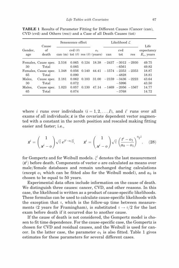
Experimental data often include information on the cause of death.We distinguish three causes: cancer, CVD, and other reasons. In thiscase, the likelihood is written as a product of cause-specific likelihoods.These formulas can be used to calculate cause-specific likelihoods withthe exception that s, which is the follow-up time between measure-ments (2 years for Framingham), is substituted s ! s=2 for the lastexam before death if it occurred due to another cause.

If the cause of death is not considered, the Gompertz model is cho-sen to fit time dependence. For the cause-specific case, the Gompertz ischosen for CVD and residual causes, and the Weibull is used for can-cer. In the latter case, the parameter o1 is also fitted. Table 1 givesestimates for these parameters for several different cases.

TABLE 1 Results of Parameter Fitting for Different Causes (Cancer (can),CVD (cvd) and Others (res)) and a Case of all Death Causes (tot)

Gender,age

Causeof

death

Senescence effect

o1(years)

Likelihood LLife

expectancyEx, years

cvd (h) cvdcan (m) tot (h) res (h) can tot res

Females,30

Cause spec. 2.516 0.065 0.124 18.38 �2437 �3012 �2930 49.75Total 0.085 �6561 49.82

Females,65

Cause spec. 1.348 0.056 0.140 44.41 �1574 �2353 �2353 18.87Total 0.090 �4828 18.81

Males,30

Cause spec. 2.181 0.062 0.103 31.00 �2159 �3436 �2223 43.64Total 0.072 �5996 43.50

Males,65

Cause spec. 1.023 0.057 0.130 47.14 �1469 �2056 �1567 14.77Total 0.074 �3768 14.72


Linear Model and Cross Check

A linear dynamic model is convenient object because life table func-tions can be calculated using both analytic methods and numericalmicrosimulations. Results of these two approaches must coincide inthe limit of large cohort size. This fact can be used to test the microsi-mulation approach. First, an analytical test is performed. We demon-strate that the standard expressions (7) for distribution moments willhold if we use our simulation method. Expression for the means n�t ofthe survival distribution is obtained using Eq. (18) and (8),

n�t ¼Z

dxt xt pGðxt; n�t ;V�t Þ ¼

Zdxt xt

l�tlt

pGðxt; nt;VtÞ e�lt

¼ ð1þ VtBtÞ�1ðnt � VtbtÞ ¼ nt � V�t ðbt þ BtntÞ:

Other quantities can be calculated in a similar fashion.The second step is a numerical comparison. We assume that

all individuals in the initial cohort are distributed according to amultivariate normal distribution. Then individual trajectories aresimulated and observable quantities are calculated, as discussedabove. Mean values and the variance-covariance matrix of an initialcohort are used for life table projection calculations. Comparing theresults, we found that the theoretical (life table) and simulated sur-vival functions and projections for all xt coincide up to statisticaluncertainties.

Nonlinear Model

Various nonlinear models applied to the Framingham data were inves-tigated in Kulminski et al. (2004). It was shown that nonlinear modelsdescribe data much better by considering risk factor interactions. Themost satisfactory nonlinear model of the second order is the model inwhich coefficients for the squares of cigarette smoking and LVH areset to zero. It was also concluded that risk factor dynamics for femalesare more complicated than for males, i.e., female health is more sensi-tive to the nonlinear interactions among risk factors.

We extend this analysis, generalizing it to take into accountmortality. Since the analysis of the residuals of the nonlinear modelshows that the statistical criteria of the quality of regression modelsare not satisfactory for cigarette smoking and LVH for projecting fromage 30, we will use two models in further analyses. One of them (M11)is a full model with all covariates. In another model (M9) these twocovariates are excluded. Statistical criteria (AIC, BIC and likelihoodratio tests) confirm that the linear model has an insufficient numberof parameters. In M11 the double difference of (log)likelihoods


2ðlogLnon2 � logLlin

2 Þ is 4250 for males and 5648 for females. Thisquantity asymptotically has a v2 distribution with 640 degrees offreedom. Thus, the null hypothesis that all nonlinear contributionsare zero, has to be rejected at the 5% significance level. For M9 thesituation is similar, i.e. 2ðlogLnon

2 � logLlin2 Þ is 1918 for males and

3042 for females, with a difference in the number of parameters of320. This result is not surprising because of the large number ofmeasurements: 32,884 residuals per equation for males and 46,784for females, while the number of estimated parameters is 12 perequation in M11, and 10 in M9.

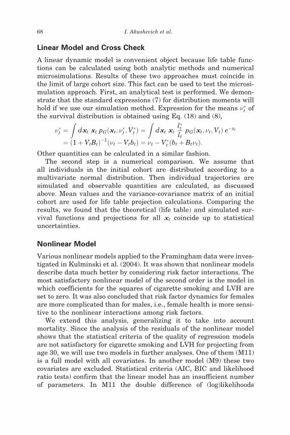
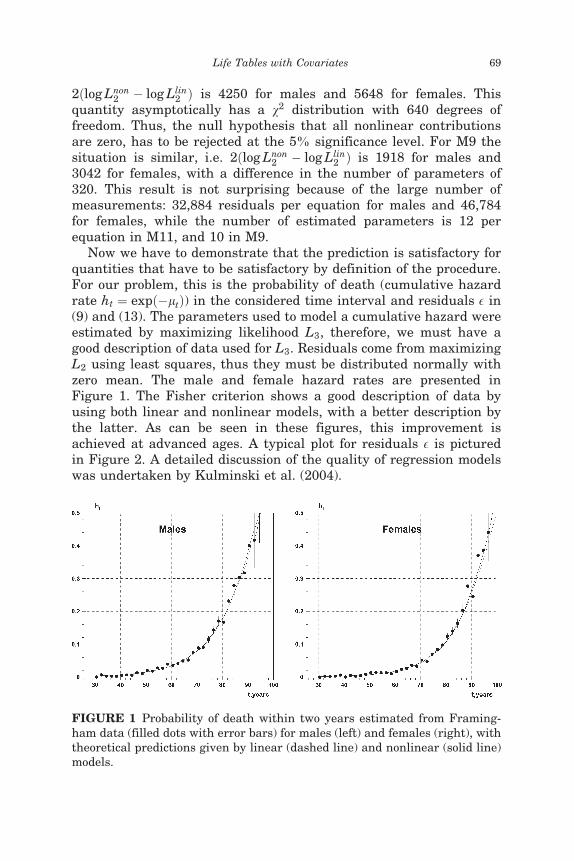
Now we have to demonstrate that the prediction is satisfactory forquantities that have to be satisfactory by definition of the procedure.For our problem, this is the probability of death (cumulative hazardrate ht ¼ expð�ltÞ) in the considered time interval and residuals E in(9) and (13). The parameters used to model a cumulative hazard wereestimated by maximizing likelihood L3, therefore, we must have agood description of data used for L3. Residuals come from maximizingL2 using least squares, thus they must be distributed normally withzero mean. The male and female hazard rates are presented inFigure 1. The Fisher criterion shows a good description of data byusing both linear and nonlinear models, with a better description bythe latter. As can be seen in these figures, this improvement isachieved at advanced ages. A typical plot for residuals E is picturedin Figure 2. A detailed discussion of the quality of regression modelswas undertaken by Kulminski et al. (2004).

FIGURE 1 Probability of death within two years estimated from Framing-ham data (filled dots with error bars) for males (left) and females (right), withtheoretical predictions given by linear (dashed line) and nonlinear (solid line)models.


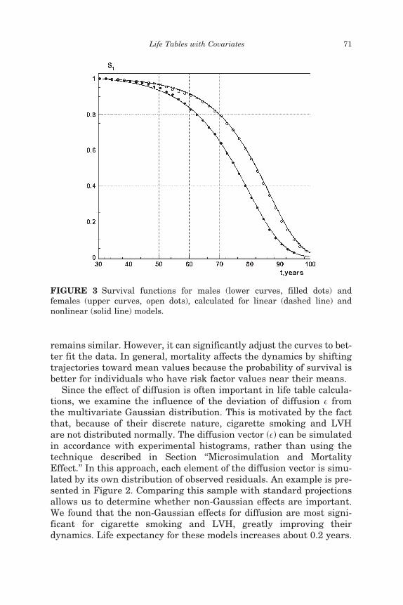
Next we focus on predicting survival functions and on projectingrisk factors. The results are presented in Figures 3, 4 and 5 for linearand nonlinear models. The survival functions predicted by linear andnonlinear models (Figure 3) are nearly identical. This is not surpris-ing, since the same hazard parameters are used in both models andthe survival functions can differ only due to the different covariate dis-tributions used in Eq. (6). Only for advanced ages (90þ) does the non-linear model predict a slightly smaller percent of survival. This is theconsequence of the increased hazard rate shown in Figure 1. Lifeexpectancies are provided in Table 1.

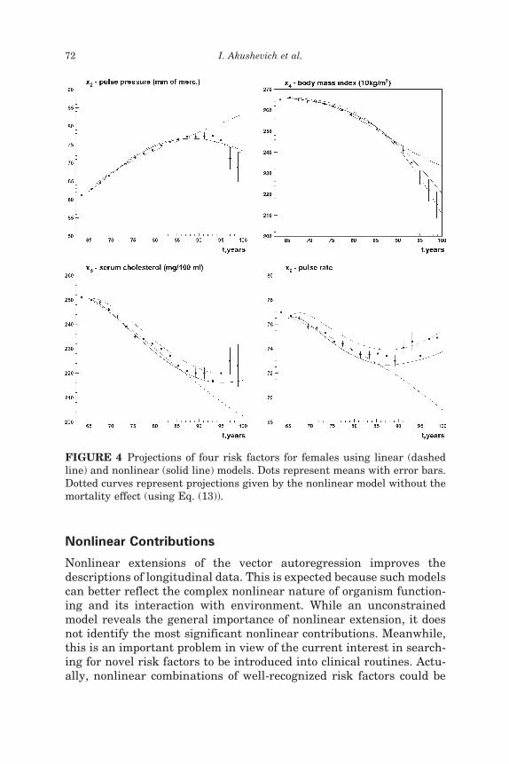
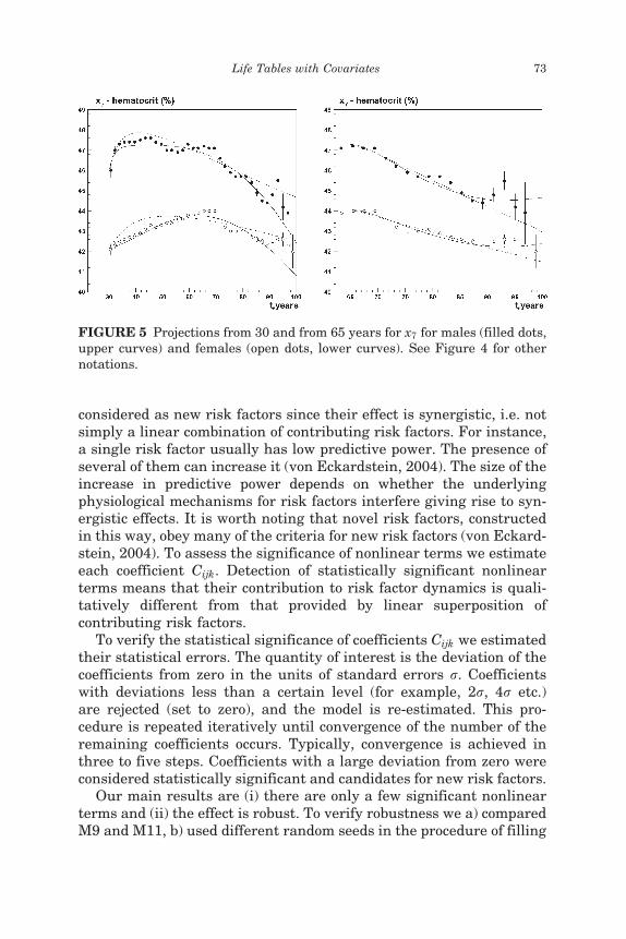
The analysis of dynamics (Figures 4 and 5) suggests that the non-linear model is more suitable for describing covariate dynamics thanthe linear one. Nonlinear effects are especially important at advancedages (Figure 4). For these ages the linear model can capture neitherthe shape nor the values of the projected risk factors. Figure 5 demon-strates the projections for hematocrit from age 30 and 65 years. Thecomparison of these two plots shows that the domain of advanced agesis fitted much better by nonlinear models.

Predictions of the nonlinear model without mortality effects are alsoplotted in Figure 4. Mortality plays a minor role in dynamics and doesnot qualitatively change propagation, i.e., the shape of the curves

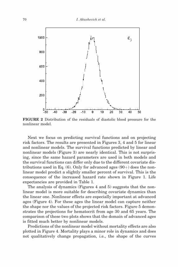
FIGURE 2 Distribution of the residuals of diastolic blood pressure for thenonlinear model.


remains similar. However, it can significantly adjust the curves to bet-ter fit the data. In general, mortality affects the dynamics by shiftingtrajectories toward mean values because the probability of survival isbetter for individuals who have risk factor values near their means.

Since the effect of diffusion is often important in life table calcula-tions, we examine the influence of the deviation of diffusion E fromthe multivariate Gaussian distribution. This is motivated by the factthat, because of their discrete nature, cigarette smoking and LVHare not distributed normally. The diffusion vector (E) can be simulatedin accordance with experimental histograms, rather than using thetechnique described in Section ‘‘Microsimulation and MortalityEffect.’’ In this approach, each element of the diffusion vector is simu-lated by its own distribution of observed residuals. An example is pre-sented in Figure 2. Comparing this sample with standard projectionsallows us to determine whether non-Gaussian effects are important.We found that the non-Gaussian effects for diffusion are most signi-ficant for cigarette smoking and LVH, greatly improving theirdynamics. Life expectancy for these models increases about 0.2 years.

FIGURE 3 Survival functions for males (lower curves, filled dots) andfemales (upper curves, open dots), calculated for linear (dashed line) andnonlinear (solid line) models.


Nonlinear Contributions

Nonlinear extensions of the vector autoregression improves thedescriptions of longitudinal data. This is expected because such modelscan better reflect the complex nonlinear nature of organism function-ing and its interaction with environment. While an unconstrainedmodel reveals the general importance of nonlinear extension, it doesnot identify the most significant nonlinear contributions. Meanwhile,this is an important problem in view of the current interest in search-ing for novel risk factors to be introduced into clinical routines. Actu-ally, nonlinear combinations of well-recognized risk factors could be

FIGURE 4 Projections of four risk factors for females using linear (dashedline) and nonlinear (solid line) models. Dots represent means with error bars.Dotted curves represent projections given by the nonlinear model without themortality effect (using Eq. (13)).


considered as new risk factors since their effect is synergistic, i.e. notsimply a linear combination of contributing risk factors. For instance,a single risk factor usually has low predictive power. The presence ofseveral of them can increase it (von Eckardstein, 2004). The size of theincrease in predictive power depends on whether the underlyingphysiological mechanisms for risk factors interfere giving rise to syn-ergistic effects. It is worth noting that novel risk factors, constructedin this way, obey many of the criteria for new risk factors (von Eckard-stein, 2004). To assess the significance of nonlinear terms we estimateeach coefficient Cijk. Detection of statistically significant nonlinearterms means that their contribution to risk factor dynamics is quali-tatively different from that provided by linear superposition ofcontributing risk factors.

To verify the statistical significance of coefficients Cijk we estimatedtheir statistical errors. The quantity of interest is the deviation of thecoefficients from zero in the units of standard errors r. Coefficientswith deviations less than a certain level (for example, 2r, 4r etc.)are rejected (set to zero), and the model is re-estimated. This pro-cedure is repeated iteratively until convergence of the number of theremaining coefficients occurs. Typically, convergence is achieved inthree to five steps. Coefficients with a large deviation from zero wereconsidered statistically significant and candidates for new risk factors.

Our main results are (i) there are only a few significant nonlinearterms and (ii) the effect is robust. To verify robustness we a) comparedM9 and M11, b) used different random seeds in the procedure of filling

FIGURE 5 Projections from 30 and from 65 years for x7 for males (filled dots,upper curves) and females (open dots, lower curves). See Figure 4 for othernotations.


missing data, c) applied hard (i.e., 4r) and soft (iterations from 1r to4r) criteria, d) combined several tests simultaneously. In all of themthe pattern of nonlinear terms with a significance level greater than4r remained similar. Nevertheless, the set of significant coefficientswas age- and sex-dependent that is physiologically justified. We visu-ally inspected trajectories for risk factors to verify the quality of thepropagation. This test shows that, as a rule, projected curves of meansdo not become worse. In some cases we even observed that propagationbecomes slightly better and smoother.

Although we tested nonlinear contributions, an important problemis the significance of linear terms and whether they should be retainedindependently of significance or neglected. If non-significant linearterms are neglected, it affects the distribution of the significance ofnonlinear terms because the function of neglected linear terms istransferred to corresponding nonlinear terms. Therefore, by neglect-ing linear terms we cannot claim a pure nonlinear effect. Thus, inour analysis of statistically significant nonlinear terms, we use amodel in which all linear terms are kept, i.e., a nonlinear model withan unconstrained linear part.

This model was used to iteratively extract significant nonlinear con-tributions for two starting projection ages, apr, (30 and 65) and bothsexes. Since the statistics in all four cases are different, the signifi-cance level at which iterations were stopped was different. Specifi-cally, it was 9r for females for apr � 30, 7r for females for apr � 30,and 5r for apr � 65 and both sexes.

We identify several groups of significant nonlinear terms (seeTable 2). The first group (I) includes contributions with age squared(Ci11). Their appearance is sensitive to the starting projection age.For projections starting at 30 years (apr � 30) significant coefficientsare detected for diastolic blood pressure (i ¼ 3) and serum cholesterol(i ¼ 5) for both sexes and, in addition, for body mass index (i ¼ 4) andhematocrit (i ¼ 7) for females. For projections starting at 65 (apr � 65)significant contributions are detected only for females, C211 (pulsepressure). The second group (II) contains age-independent diagonal(Ciii, i 6¼ 1) and non-diagonal (Cjii, j; i 6¼ 1) squares. The most signifi-cant diagonal contribution is the pulse rate (i ¼ 9). Others are vitalcapacity index (i ¼ 8), body mass index (i ¼ 4), blood glucose (i ¼ 6)and hematocrit (i ¼ 7). A significant non-diagonal coefficient is C322

for males for apr � 30. The third group (III) includes diagonal andnon-diagonal age and non-age-covariate interaction terms (Ci1i andCj1i, j; i 6¼ 1). The serum cholesterol coefficient C515 is significant inalmost all cases with the exception for females (apr � 65), where itwas rejected at the level of 3r. This is the only contribution of this


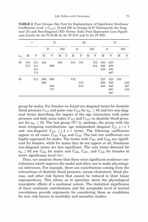
group for males. For females we found two diagonal terms for diastolicblood pressure C313 and pulse rate C919 for apr � 65 and two non-diag-onal terms describing the impact of the age interaction with pulsepressure and body mass index (C312 and C314) on diastolic blood press-ure for apr � 30. The last group (IV) is, perhaps, the group with themost intriguing contributions: age independent diagonal Cjji, j; i 6¼ 1and non-diagonal Cjik, j; i; k 6¼ 1 terms. The following coefficientsappear in all cases: C223, C626 and C646. The last two coefficients arehighly expressed for males. The terms with C667 and C668 are signifi-cant for females, while for males they do not appear at all. Nonlinearnon-diagonal terms are less significant. The only terms detected forapr � 65 are C526 for males and C236, C467, and C539 for females atlower significance level (3r).

Thus, our analysis shows that there exist significant nonlinear con-tributions which improve the model and allow one to make physiologi-cal inferences. For example, there are contributions coming from theinteractions of diastolic blood pressure, serum cholesterol, blood glu-cose, and other risk factors that cannot be reduced to their linearsuperpositions. This allows us to speculate about the physiologicalsynergistic effects of a nonlinear nature. The statistical significanceof these nonlinear contributions and the acceptable level of mutualcorrelations provide arguments for considering them as candidatesfor new risk factors in morbidity and mortality studies.

TABLE 2 Four Groups (See Text for Explanations) of Significant NonlinearCoefficients (mnk � Cmnk). D and ND in Groups II-IV Distinguish the Diag-onal (D) and Non-Diagonal (ND) Terms. Italic Font Represents Less Signifi-cant Levels (6r for IV-D-M; 8r for IV-D-F and 3r for IV-ND)

apr

I II III IV

D ND D ND D ND

M F M F M F M F M F M F M F

30 311 311 444 322 515 515 312 223 223511 511 999 314 626 626

411 646 646711 667

65 211 999 999 515 223 223 526666 313 626 626 236

888 919 646 646 467777 667 539

667


Note that the next natural step would be extending the quadratichazard model to include these novel risk factors and verifying theirimpact on survival. This would lead to a mortality model of the fourthdegree, which is not purely quadratic. This can be a subject of futurework when more complete data from the Framingham Study are avail-able. The statistical criteria applied to our current data show that wedo not have a deficit of survival parameters.

Interventions

Manton et al. (1992) showed that the effects of interventions affectinghealth status can be studied by changing regression u, R, R or hazardQ parameters, as well as initial conditions nt0 and Vt0 . A comparison ofthe projected results (e.g., life expectancies) allows one to make conclu-sions about the impact of interventions on health. Microsimulationallows us to advance this technique by using individual (or xt-depen-dent) interventions that are more realistic and flexible. The simplestway to introduce interventions at the individual level is to use specificcuts for the simulated values of risk factors or for the diffusion vector E.These cuts can be age-, gender-, race- or covariate-dependent. Forexample, a restriction in cigarette smoking can be analyzed by requir-ing x11 < 15. Another example is to use a cut on a specific component ofthe diffusion vector E.

Strictly speaking, any cuts on the components of covariate or dif-fusion vectors, applied to real data, change the regression estimatesand the hazard parameters, both of which are used for projections.Thus an exact method of x-dependent intervention treatment has toinclude iterative compensations for these deviations. The first step isto fix a desirable intervention and to calculate the zeroth approxi-mation for the dynamic and survival curves. The simulated risk fac-tors for the cohort can be treated as a new cohort and used tocalculate new mortality coefficients and regression matrices. This pro-cedure can be iteratively repeated until convergence occurs. Insightscan be obtained at the zeroth step of this iterative procedure, as illu-strated below.

We consider three examples. First, we restrict cigarette smoking toa limit of x11 < 15 cigarettes per day for males and females of all ages.Second, we increase the diffusion for VCI by a factor of 2. Since VCIcan be considered as a biomarker of senescence, this intervention cor-responds to the case of a sub-population with accelerated aging.Finally, we perform an intervention describing blood pressure control,i.e., the diffusion vectors for pulse pressure and diastolic blood press-ure are lowered by a factor of 2.


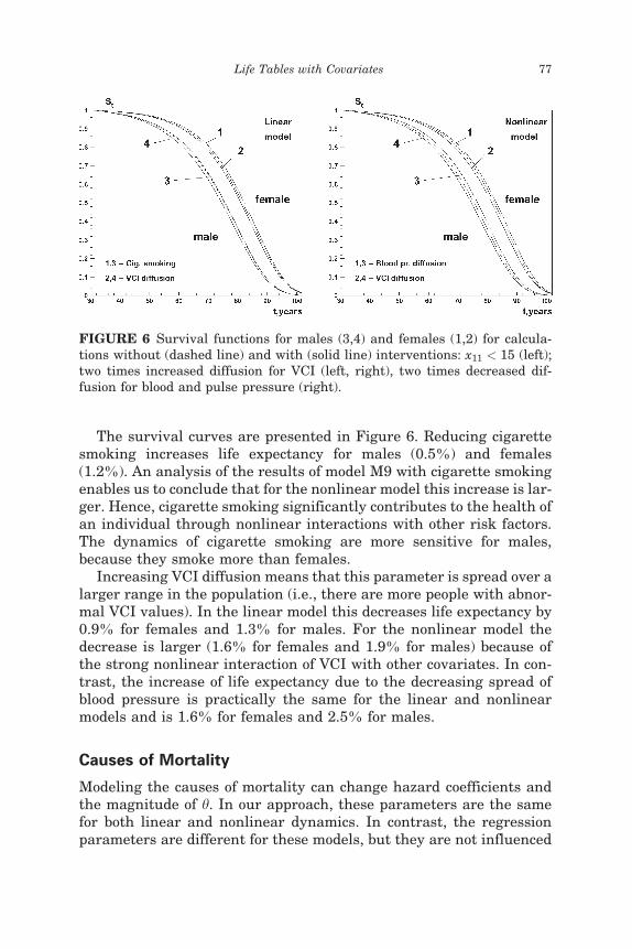
The survival curves are presented in Figure 6. Reducing cigarettesmoking increases life expectancy for males (0.5%) and females(1.2%). An analysis of the results of model M9 with cigarette smokingenables us to conclude that for the nonlinear model this increase is lar-ger. Hence, cigarette smoking significantly contributes to the health ofan individual through nonlinear interactions with other risk factors.The dynamics of cigarette smoking are more sensitive for males,because they smoke more than females.

Increasing VCI diffusion means that this parameter is spread over alarger range in the population (i.e., there are more people with abnor-mal VCI values). In the linear model this decreases life expectancy by0.9% for females and 1.3% for males. For the nonlinear model thedecrease is larger (1.6% for females and 1.9% for males) because ofthe strong nonlinear interaction of VCI with other covariates. In con-trast, the increase of life expectancy due to the decreasing spread ofblood pressure is practically the same for the linear and nonlinearmodels and is 1.6% for females and 2.5% for males.

Causes of Mortality

Modeling the causes of mortality can change hazard coefficients andthe magnitude of h. In our approach, these parameters are the samefor both linear and nonlinear dynamics. In contrast, the regressionparameters are different for these models, but they are not influenced

FIGURE 6 Survival functions for males (3,4) and females (1,2) for calcula-tions without (dashed line) and with (solid line) interventions: x11 < 15 (left);two times increased diffusion for VCI (left, right), two times decreased dif-fusion for blood and pulse pressure (right).


by mortality causes. Thus, the dynamics and survival functions for thecause-specific case reflect all features of the total (cause averaged)case. Numerical analysis confirms this conclusion. The dynamics atearly ages predicted by the linear model is nearly the same as in thestandard Gompertz model for all causes of deaths. At advanced ages,it can deviate significantly. The survival curves essentially coincidewith those for the cause-averaged model, so life expectancy differslittle (less than 0.1 year). Nonlinear interactions can give rise tonoticeable differences for both dynamics and survival curves. Lifeexpectancy is nearly equal to that of the linear model. However, non-linear corrections have opposite signs for males and females. Forfemales life expectancy is smaller when compared to the linear model.The opposite is found for males.

CONCLUSION

We generalized the population life table model by Woodbury and Man-ton (1977, 1983), which is based on a system of stochastic differentialIto equations for linear dynamics and mortality selection. The assump-tion about linear dynamics restricts the accuracy and predictive powerof this model. Kulminski et al. (2004) suggested a nonlinear model forlongitudinal data to reflect risk factor interactions. The system of fivedifference equations in the model of Woodbury and Manton (1983) can-not be generalized to this class of nonlinear models due to the lack ofnormality in propagating the population distribution. In this paper,we describe how to generalize the model for the dynamics of any com-plexity by using a formalism based on the microsimulation of individ-ual trajectories. This formalism gives exact results for projection ofpopulation trajectories and survival functions in the limit of largecohort size. Since microsimulation deals with individual trajectories,the effects of health interventions and the influences of assumptionsabout linear dynamics and Gaussian diffusion on life expectancy canbe studied.

This approach was applied to a dynamic model with second ordernonlinearities. The strategy of parameter estimation is describedand the necessary properties of the likelihood function are illustrated.Data analysis of the 46-year follow-up of the Framingham HeartStudy showed that the nonlinear model fits the data much better,especially at advanced ages. We analyzed the effects of non-Gaussiandiffusion. These effects provide a more accurate dynamic model for dis-crete risk factors (cigarette smoking, LVH). We identified a set of stat-istically significant nonlinear combinations of risk factors in the senseof their influence on risk factor dynamics. The influence of these terms


could not be reduced to the linear superposition of contributing riskfactors. This reflects the synergistic nature of covariate interactionsand allows one to consider significant nonlinear contributions as can-didates for new risk factors in morbidity and mortality studies. Wealso illustrate the effects of interventions on risk factors and their dif-fusion. These calculations provide the background for forecasting andactuarial calculations.

This class of models allows one to investigate more realistic assump-tions about changes in health, as indexed by major risk factors andmortality. It will also help us to understand the mechanisms of healthchanges both at the individual level and for populations. An approachemploying joint analysis of the effects of risk factors and mortalitywith their interactions is an important step in eliminating the pro-blems of demographic models when only mortality models are usedto describe and project health changes.

REFERENCES

Akushevich, I., Akushevich, L., Manton, K.G., and Yashin, A. (2003). Stochastic processmodel of mortality and aging: application to longitudinal data. Nonlinear Phenomenaand Complex Systems 6: 515–523.

Carey, J.R., Liedo, P., Orozco, D., and Vaupel, J.W. (1992). Slowing of mortality rates atolder ages in large medfly cohorts. Science 258: 457–461.

Dubey, S.D. (1967). Some percentile estimators of weibull parameters. Technometrics 9:119–129.

Kloeden, P.E. and Platen, E. (1992). Numerical Solution of Stochastic Differential Equa-tions. Application of Mathematics Series Vol. 23. Heidelberg: Springer-Verlag.

Kloeden, P.E., Platen, E., and Schurz, H. (1994). Numerical Solution of SDE ThroughComputer Experiments. Berlin: Springer.

Kulminski, A., Akushevich, I., and Manton, K. (2004). Modeling nonlinear effects inlongitudinal survival data: implications for the physiological dynamics of biologicalsystems. Frontiers in Bioscience 9, 481–493, special issue, http:==www.bioscience.org=current=special=manton.htm.

Lew, E.A. and Garfinkel, L. (1984). Mortality ages 65 and over in a middle-class popu-lation. Trans. Soc. Actuaries 36: 257–295.

Lew, E.A. and Garfinkel, L. (1987). Differences in mortality and longevity by sex, smok-ing habits and health status. Trans. Soc. Actuaries 39: 107–125.

Manton, K.G., Stallard, E., and Vaupel, J.W. (1986). Alternative models for theheterogeneity of mortality risks among the aged. Journal of the American StatisticalAssociation 81: 635–644.

Manton, K.G. and Stallard, E. (1988). Chronic Disease Modeling: Measurement andEvaluation of the Risks of Chronic Disease Processes. London: Griffin; New York:Oxford University Press.

Manton, K.G., Stallard, E., and Singer, B. (1992). Projecting the future size and healthstatus of the US elderly population. International Journal of Forecasting 8: 433–458.

Manton, K.G., Stallad, E., Woodbury, M.A., and Dowd, J. (1994). Time-varying covari-ates in models of human mortality and aging: multidimensional generalizations ofthe Gompertz. Journal of Gerontology: Biological Sciences 49: B169–B190.


Manton, K.G. (1999). Dynamic paradigms for human mortality and aging. Journal ofGerontology: Biological Sciences 54A: B247–B254.

Manton, K.G. and Yashin, A.I. (2000). Mechanisms of Aging and Mortality: The Searchfor New Paradigms. Denmark: Odense University Press.

Michalski, J.M., Winter, K., Purdy, J.A., Wilder, R.B., Perez C.A., Roach., M. et al.(2003). Preliminary evaluation of low–grade toxicity with conformal radiation ther-apy for prostate cancer on RTOG 9406 dose levels I and II. International Journalof Radiation Oncology, Biology, Physics 56: 192–8.

Orchard, G. and Woodbury, M.A. (1971). A missing information principle: Theory andapplication. In L. LeCam, J. Heyman, and E. Scott (Eds.), Sixth Berkley Symposiumon Mathematical Statistics and Probability. Berkley, CA: University of CaliforniaPress, pp. 697–715.

Pe~nna, D., Tiao, G.C., and Tsay, R.S. (2001). A Course in Time Series Analysis. New York,NY: Wiley.

Risken, H. (1989). The Fokker-Planck Equation: Methods of Solution and Applications.New York, NY: Springer-Verlag.

Stebbing, A.R.D. (1987). Growth hormesis: a by-product of control. Health Physics 52:543–547.

Vaupel, J.W. and Yashin, A.I. (1985). Heterogeneity’s ruses: some surprising effects ofselection on population dynamics. The American Statistician 39: 176–185.

von Eckardstein A. (2004). Is there a need for novel cardiovascular risk factors? NephrolDial Transplant. Apr 19(4): 761–5.

Witteman, J.C.M., Grobbee, D.E., Valkenburg, H.A., van Hemert, A.M., Stijnen, T.,Burger, H., Hofman, A. (1994). J-shaped relation between change in diastolic bloodpressure and aortic atherosclerosis. Lancet 343: 504–507.

Woodbury, M.A. and Manton, K.G. (1977). A random walk model of human mortalityand aging. Theoretical Population Biology 11: 37–48.

Woodbury, M.A. and Manton, K.G. (1983). A theoretical model of the physiologicaldynamics of circulatory disease in human populations. Human Biology 55: 417–441.

Woodbury, M.A., Manton, K.G., and Stallard, E. (1981). Longitudinal models for chronicdisease risk: an evaluation of logistic multiple regression and alternatives. Inter-national Journal of Epidemiology 10: 187–197.

Wolf, D. (2001). The role of microsimulation in longitudinal data analysis. CanadianStudies in Population 28: 165–179.

Yashin, A. and Arjas, E. (1988). A note on random intensities and conditional survivalfunctions. Journal of Applied Probability 25: 630–635.

Yashin, A.I., Iachine, I.A., and Begun, A.S. (2000). Mortality Modeling: A Review.Mathematical Population Studies 8(4): 305–332.


Documents

Life Tables with Covariates: Dynamic Model for Nonlinear Analysis of Longitudinal Data