Embed Size (px)
Citation preview

DI
SC
US
SI
ON
P
AP
ER
S
ER
IE
S
Forschungsinstitut zur Zukunft der ArbeitInstitute for the Study of Labor
Life Satisfaction, Income and Personality
IZA DP No. 8837
February 2015
Eugenio ProtoAldo Rustichini

Life Satisfaction, Income and Personality
Eugenio Proto University of Warwick
and IZA
Aldo Rustichini University of Minnesota
Discussion Paper No. 8837 February 2015
IZA
P.O. Box 7240 53072 Bonn
Germany
Phone: +49-228-3894-0 Fax: +49-228-3894-180
E-mail: [email protected]
Any opinions expressed here are those of the author(s) and not those of IZA. Research published in this series may include views on policy, but the institute itself takes no institutional policy positions. The IZA research network is committed to the IZA Guiding Principles of Research Integrity. The Institute for the Study of Labor (IZA) in Bonn is a local and virtual international research center and a place of communication between science, politics and business. IZA is an independent nonprofit organization supported by Deutsche Post Foundation. The center is associated with the University of Bonn and offers a stimulating research environment through its international network, workshops and conferences, data service, project support, research visits and doctoral program. IZA engages in (i) original and internationally competitive research in all fields of labor economics, (ii) development of policy concepts, and (iii) dissemination of research results and concepts to the interested public. IZA Discussion Papers often represent preliminary work and are circulated to encourage discussion. Citation of such a paper should account for its provisional character. A revised version may be available directly from the author.

IZA Discussion Paper No. 8837 February 2015
ABSTRACT
Life Satisfaction, Income and Personality We use personality traits to better understand the relationship between income and life satisfaction. Personality traits mediate the effect of income on life satisfaction. The effect of neuroticism, which measures sensitivity to threat and punishment, is strong in both the British Household Panel Survey and the German Socioeconomic Panel. Neuroticism increases the usually observed concavity of the relationship: individuals with a higher neuroticism score enjoy extra income more than those with a lower score if they are poorer, and enjoy extra income less if they are richer. When the interaction between income and neuroticism is introduced, income does not have a significant effect on its own. To interpret the results, we present a simple model based on Prospect Theory, where we assume that: (i) life satisfaction is dependent on the gap between aspired and realized income, and this is modulated by neuroticism; and (ii) income increases in aspirations with a slope less than unity, so that the gap between aspired and realized income increases with aspirations. From the estimation of this model we argue that poorer individuals tend to over-shoot in their aspirations, while the rich tend to under-shoot. The estimation of the model also shows a substantial effect of traits on income. JEL Classification: D03, D87, C33 Keywords: life satisfaction, income, personality traits, neuroticism, prospect theory Corresponding author: Eugenio Proto University of Warwick Department of Economics Coventry CV4 7AL United Kingdom E-mail: [email protected]

1 Introduction
Given its importance for welfare analysis and public policy, the general relation between self-
reported well-being and personally available income has been widely investigated. A regression
of life satisfaction on income using both cross-sectional and panel survey data from a developed
country generally shows a significant, positive, but small estimated coefficient of income (e.g.
Blanchflower and Oswald, 2004; Ferrer-i-Carbonell and Frijters, 2004). Although the debate
on the existence of a satiation point is still open, there is general agreement that the size of the
effect is decreasing with income, consistent with the usual assumptions on the utility function
of individuals, as Layard et al. (2008) explicitly point out.1
However, a significant amount of evidence suggests that the link between income and life
satisfaction is more complex than that. Life satisfaction appears to be monotonically increasing
with income when one studies this relation at a point in time across nations (e.g. Deaton,
2008; Stevenson and Wolfers, 2008). Over time, however, the relation between GDP and life
satisfaction appears rather different. In a well-known finding, Easterlin reports no significant
relationship between happiness and aggregate income in time-series analysis. For example, the
income per capita in the USA in the period 1974-2004 almost doubled, but the average level
of happiness shows no appreciable trend upwards. This puzzling finding, appropriately called
the Easterlin Paradox (Easterlin, 1974) has been confirmed in similar studies by psychologists
(Diener et al., 1995) and political scientists (Inglehart, 1990), and has been shown to also hold
for European countries (Easterlin, 1995).2 A recent paper by Proto and Rustichini (2013)
finds a positive relationship between growth and satisfaction for countries with a GDP below
15,000 USD but shows that this relationship is flat in richer countries, suggesting a gap between
aspiration and realised income.
A potential explanation of the paradox is that individuals adapt to current conditions, and
the level of subjective well-being tends to revert to a baseline level depending on a reference
1Layard et al. (2008) find that marginal life satisfaction with respect to income declines at a faster rate thanthat implied by a logarithmic utility function. Kahneman and Deaton (2010) argue that the effect of incomeon an emotional dimension of well-being, like happiness self-reports, reaches a maximum at an annual incomeof 75,000 USD, and it has no further positive influence for higher values; while the non-emotional measures ofwell-being like the Cantrill ladder do not feature this satiation point
2There is some disagreement in the time-series based analyses: Oswald (1997) shows evidence of a smallpositive temporal correlation between life satisfaction and GDP in industrialized countries and Stevenson andWolfers (2008) find significant happiness gains in Japan in the post-war period.
2

point, an idea originally proposed by Brickman and Campbell (1971). Aspirations are naturally
associated with the reference point provided by current income. Hence, to the extent that an
increase in income leads to an increase in aspirations, changes in income may not have a long-
run effect on subjective wellbeing.3 Another explanation of the Easterlin Paradox hinges on the
concept that relative, rather than absolute income, is the main determinant of life satisfaction,
an idea that can be dated back to Duesenberry (1949). The two explainations are closely
related.4
The present paper aims to shed more light on the relation between personal income and
life satisfaction by analyzing how personality affects this relation. Recently, economists have
recognized the importance of introducing personality traits into economic models (Borghans et
al., 2008; Rustichini, 2009; Almlund et al., 2011). Recent studies show that personality has a
biological basis, as DeYoung and Gray (2010) argue in an exhaustive survey of the literature.
The rest of the paper is organized as follows. In section 2 we describe the datasets, the
main variables (2.1) and the econometric model (2.2). In section 3 we show the results from
the estimation of the econometric model. In section 4 we describe our theory and estimate
the structural model (4.1). In section 5 we discuss the main results and conclude. Additional
analysis and more technical details are in the appendix.
2 Data and Methods
2.1 Data
We use two national data sets: the British Household Panel Survey (BHPS), covering the
years 1996-2008 (the question on life satisfaction was introduced in 1996), and the German
Socioeconomic Panel Study (SOEP), available for the years 1984-2009. Both SOEP and BHPS
are longitudinal datasets, with the same individuals interviewed every year. Summary statistics
relating to all the main variables are presented in tables 1 and 2. We now provide a brief
3Easterlin (2005), Stutzer (2004) and McBride (2010) provide some empirical evidence on how aspirationsincrease in income, Di Tella et al. (2010) show evidence that individuals adapt to status, although they cannotreject the hypothesis of no full adaptation to a change in income in four years.
4Clark and Oswald (1996), Blanchflower and Oswald (2004), Ferrer-i-Carbonell, (2005), Luttmer (2005) andSenik (2009), among others, present empirical validations of this hypothesis. See Clark et al. (2008) for anextensive survey of the theoretical and empirical literature explaining the Easterlin Paradox.
3

description of the main variables.
Big 5 Personality Traits. The Big Five are usually measured through self-report based
on the NEO Five-Factor Inventory (see e.g. Costa and McCrae, 1992). There is a large
literature demonstrating the reliability of this questionnaire and the stability of the personality
traits. The data used in the current paper have been elaborated from the standard short
questionnaire present in the BHPS and SOEP datasets (in the year 2005). Personality traits
are usually assessed with the NEO-Five Factor Inventory (NEO-FFI) with 60 items (12 items
per domain). However, recent scale-development studies have indicated that the Big Five
traits can be reliably assessed with a smaller number of items (e.g., Gosling et al., 2003). For
instance, pilot work from the German Socio-Economic Panel (GSOEP) study led to a 15-item
version of the well-validated Big Five Inventory (Benet-Martinez and John, 1998) that can be
used in large-scale surveys. The questions are presented in section A of the appendix.
We use data on the Big Five personality traits in the 2005 waves of the BHPS and SOEP
datasets as measures of individuals’ personality for the entire time span that we observe each
individual for. Borghans et al. (2008) argue that personality traits vary little for individuals
aged between 18 and 65, the life span we are considering. Our data are consistent with this
result since when we regress the personality traits against age and age squared we find that
they explain a very small portion of the variance. For example in a regression of neuroticism
with age and age2, the R2 = 0.0027 in the SOEP and R2 = 0.0025 in the BHPS. The effect on
all other traits is very similar. Although it is unlikely that this variation can bias our estimates,
in our analysis we use the residuals after controlling for the age effects. Accordingly, our results
refer to the age-invariant factor of the personality trait, which as we argued above, explains
more than 99 percent of the total variance.5
Furthermore, considering the data related to one year rather than time-changing measures
generally avoids the problem that the estimation can be biased by short-term fluctuations that
contemporaneously affect income, life satisfaction and personality. A final concern might be
related to some external shock that permanently changes personality, income and life satis-
faction. In this respect, Cobb-Clark et al. (2011), using data from two separate waves of the
5Our estimates are generally robust to the inclusion of the raw data instead of the residuals.
4

Household, Income and Labour Dynamics in Australia (HILDA) survey measuring personality,
show that that personality traits only change after main life shocks to a negligible extent. For
example, individuals who experience five or more employment/income-related negative shocks
like worsening finances, retiring, being fired, or becoming unemployed, between 2006 and 2009
(in their data more than three standard deviations) become more neurotic in the order of 0.28
standard deviations for men and 0.15 for women. Cobb-Clark et al. quantify this effect con-
sidering the usual estimated effect of traits on income (see e.g. Mueller and Plug (2006), and
also our estimation below) in a decrease of 0.012 USD in the hourly wage.
Life satisfaction. In the BHPS, the life satisfaction question is: “How dissatisfied or
satisfied are you with your life overall?” and it is coded on a scale from 1 (not satisfied at all)
to 7 (completely satisfied). In the SOEP, the questions is “We would like to ask you about your
satisfaction with your life in general”, coded on a scale from 0 (completely dissatisfied) to 10
(completely satisfied).
We present the percentage of responses in each category for both datasets in figure A.1
of the appendix. To ease comparability of the statistical results for different datasets, we
have transformed the measures of life satisfaction to always lie in a range between 1 and
7. In particular, we transform the index of the SOEP survey according to the formula 1 +
life satisfaction ×610 .
Household income. In both the SOEP and the BSHP datasets income has been converted
into USD at 2005 constant prices, using the Consumer Price Index (CPI) of the World Bank-
World Development indicators. Data on income are all in 10K units. Figure A.2 in the
appendix displays the histograms of income distributions for the UK and Germany. As is
common in the literature analyzing the effect of life satisfaction at the individual levels (e.g.
Oswald and Blanchflower, 2004; Ferrer-i-Carbonel, 2005), we use household income instead of
personal income. It is natural to conjecture that in a household there are significant amounts
of income transfers between the members; at the same time personal income earning decisions
are dependent on the income earned by the other members of the household. Considering only
personal income would have implied the exclusion of these pervasive externalities.
Control variables. Unless explicitly stated otherwise, in all regressions we control for the
5

usual demographic variables: age, age2 and gender, marital status (a set of dummies depending
on whether the respondent is married, divorced, separated or widowed), number of children
in the household, the highest academic qualifications based on the education systems of the
two countries (a set of dummies measuring high school achievement, vocational training or
college degree). In addition, we introduce, as a control for health status, a set of dummies
indicating the number of visits to the doctor. We use this variable for two reasons: (i) it is an
objective indicator of health;6 and (ii) it is present in both the SOEP and the BHPS datasets
in a similar form. We also introduce a dummy for region of residence of the household; the
regional aggregation in Germany in the SOEP dataset is based on the NUTS 1 code of the
European Union (16 regions), while for the UK data in the BHPS dataset it roughly follows
the NUTS 2 code (18 regions). Finally, we control for a series of labour environment-related
variables: labour force participation (a set of dummies depending on whether the individual
labour market status is employed, housekeeper, unemployed, retired); occupation types (a
standard set of dummies for socioeconomic status: manager, professional, white collar, blue
collar, farm worker and so on), hours worked per week and the latter squared.7
2.2 Econometric Specification
We use a quadratic specification for a model linking income to life satisfaction because we
are interested in analyzing how prsonality traits influence the concavity of this relation. In
order to avoid the excessive weight given to outliers by this specification, we exclude from the
sample the top and bottom 1 percent of observations. Excluding observations in the two tails
of income distribution is standard in this literature.8
In particular, we estimate the following model:
hit = β1yit + β2y2it + β′1θiyit + β′2θiy
2it + Γzit + Λθi + εi + ηt + eit (1)
6This avoids possible biases from introducing a subjective variable in the RHS of a happiness equation.7When an individual is recorded as unemployed for employment status, she is recorded with 0 hours worked,
and he/she is recorded as unemployed also in occupation types.8For example, in the SOEP this excludes 3964 observations with an income between 114K and 1,515K at
the top and at the bottom 4019 observations with an income less than or equal to 7,277 euro per year. All thefollowing results are robust to different thresholds of exclusion.
6

In equation (1), i represents the individual and t the year of the survey, hit is life satisfaction
and yit household income. The individual fixed effect is described as Λθi + εi, where
θi = (Ni, Ei, Ci, Ai, Oi,Mi) (2)
with N = Neuroticism, E = Extraversion, C = Conscientiousness, A = Agreeableness,
O = Openness, M = Male and εi is the individual specific random effect. The terms β′1θiyit+
β′2θiy2it represent the interaction of a personality trait index with the income variables. The
vector zit consists of time-changing individual characteristics. The variable ηt denotes a year
(and wave) fixed effect and eit is random noise.
3 Results
Figures 1 and 2 display the residuals of life satisfaction – after controlling for age, age2, gender
and the five personality traits, as a function of income residuals after controlling for the same
variables, in the UK and Germany respectively. From the two panels in figure 1, we note that
for individuals with a high neuroticism score, the curve is more concave, while for those with
low neuroticism this relation is almost linear. Furthermore, in both countries the relation is
steeper for high neuroticism scores with respect to low neuroticism scores in the region of the
graph corresponding to lower incomes, while it is flatter for high neuroticism scores with high
income. Finally, we note from the graphs in figure 2 that no other trait has such a clear effect
on the relation we are analyzing.
The panels in Figures 1 and 2 are based on data pooled across waves. To exploit the
longitudinal nature of our dataset by taking into account individuals’ heterogeneity and to
exclude the role of omitted variables, we estimate a number of econometric models controlling
for a large number of potentially confounding factors. We estimate model (1) by OLS estimation
and report the results in table 3, where in order to take into account possible heteroscedasticity,
we cluster the standard errors at the individual levels.9 The table shows that in both datasets
9It is known in this literature that assuming ordinality or cardinality of happiness scores makes little difference(Ferrer-i-Carbonell Frijters 2004). This can also be observed in table 5, where we report the estimation of asimilar model using an ordered probit estimator.
7

neuroticism is the only one of the five personality traits to affect the relation between income
and life satisfaction, and in a qualitatively similar way. No other trait significantly interacts in
the relationship between income and life satisfaction. Furthermore, both in Germany and in
the UK, the usually observed marginal decreasing effect of income on life satisfaction is entirely
mediated by neuroticism. Once the interacted term is taken into account, either there is no
effect of income on life satisfaction or this effect becomes convex as in column 2.
A possible concern is that the random effect estimator is not consistent due to the fact
that εi is correlated with the other regressors. We therefore estimate an equation similar to
model 1 with individual fixed effects. The results are reported in table 4. Finally, we further
interact the terms neuroticism*income with a male dummy. From table 6 we note that for
males neuroticism affects the relation between income and life satisfaction more strongly than
for females. In other words, the concavity of this relation, due to the neuroticism, is stronger
among males.
Why do we observe this strong effect of neuroticism in modulating the relationship between
income and life satisfaction? Neuroticism is linked to higher sensitivity to negative emotions like
anger, hostility or depression (e.g. Clark and Watson, 2008), and is associated with structural
features of the brain systems associated with sensitivity to threat and punishment. For this
reason, modern studies identify this personality trait with sensitivity to negative outcomes,
threats and punishments (see DeYoung and Gray (2010) for a recent survey). It is therefore
reasonable to assume that people with higher neuroticism experience higher sensitivity to losses
or failure to meet their expectations, an effect similar to loss aversion in the prospect theory.
In the next section, we will therefore derive an explanation of the effect of neuroticism we see
in figure 1 and tables 4 and 6 by estimating a prospect theory-based model.
We will assume that neuroticism modulates the effect of the gap between aspired and
realized income and we show that, when aspirations are not observed, neuroticism appears to
decrease the elasticity between income and life satisfaction for high income levels and to increase
this elasticity for lower income levels, as observed in this section. Furthermore, our model below
will also explain why personality traits underlying motivation, like conscientiousness, openness
and extraversion (see e.g. DeYoung and Gray 2010) do not have an effect on the way income
8

affects life satisfaction, but they significantly affect income.
4 A model of life satisfaction, income and personality
To better understand the relation presented in the previous section between happiness, income
and personality, we present a simple structural model based on the insights deriving from the
theories of personality traits that we outlined above. We show that this model is able to
produce an equation similar to equation 1 as a reduced form and we estimate this model. We
then interpret the coefficient of the estimation in the light of the underlying structural model.
The terms eit;uit; vit are error terms. The model has three equations. The dependent
observable variables are household income yit and life satisfaction hit. The dependent latent
variable is the desired income for any individual i at time t and is denoted by ait. We assume
that the aspiration to an income, ait induces (through effort, persistence, and confidence) a
real level of income that is increasing in the aspiration level. Thus the Level of income depends
on the desired income as follows:
yit = α2 + β2ait + uit. (3)
Let α2 > 0 and β2 ∈ (0, 1), so that the aspiration to an income ait induces (through effort,
persistence, and confidence) a real level of income that is increasing in the aspiration level,
but at a rate smaller than 1. Individuals with low aspirations on average overshoot by earning
more than aspired. The linear form is for convenience: what is essential is that the relationship
is monotonic and has decreasing returns.
We summarize the argument in the following hypotheses: (i) higher motivation produces
aspiration to higher income, and hence to higher realized income; (ii) high aspirations are
necessary to become rich, but the higher they are, the more likely it is that they go unfulfilled.
The effect of aspiration on realized income therefore occurs at a decreasing rate. This is a
standard assumption. To illustrate it, consider the search for the “aspired” occupation. An
individual searching for the occupation may set a minimum level of earnings to be reached
before he or she stops searching. The higher the aspiration level the higher the final earnings
9

will be, everything else being equal, although perhaps at a later date. Increasing aspirations
may increase realized income, but, only up to a point: if they are too high they will never be
fulfilled even after a long period of searching. Note that this applies to different job statuses: for
a self-employed individual the right occupation can be found in a new project; for an employee,
the right occupation can be a promotion or a new position; for an unemployed individual or
somebody in search of a new occupation this is a new job; for a capital owner this can be the
right investment. Furthermore, we also note that the interpretation of this model can also be
extended to the marriage market, as representing the search for the right partner.
Using equation 3, it is possible to argue that this implies that the rich fail to meet their
aspirations on average more than the poor. In other words, the rich under shoot in their
aspirations on average more than poorer individuals.
A crucial assumption is that an individual’s sensitivity to the gap between aspired and
realized income depends on his/her personality. As mentioned above, recent literature in
psychology views neuroticism as sensibility to negative outcomes. Ex-post, individuals perceive
the negative gap between real and aspired income as a negative outcome, and the higher their
neuroticism score, the higher the potential subjective welfare cost of this gap. This is also an
application of prospect theory.
Accordingly we assume that life satisfaction depends on realized income and other vari-
ables, but it also depends on the distance with aspirations and this distance is modulated by
neuroticism.
hit = α1 + β1yit + δy2it + (4)
+γ1Ni (ait − yit) + γ2,1Ni[(ait − yit)+]2 +
+γ2,2Ni[(ait − yit)−]2 + Γ1zhit + Λ1θhi + eit.
where the term (ait − yit)+ is (ait − yit) when the value within brackets is positive and it is 0
when ait < yit, while (ait − yit)− is (ait − yit) when ait < yit and 0 otherwise. We expect the
term γ1 to be negative while the terms γ2,1 and γ2,2 depend on the concavity of the function. If
we consider ait as a reference point, prospect theory would predict that equation 4 is concave
10

in the “gains”, i.e. when ait < yit and convex in the “losses”, i.e. when ait > yit. Accordingly,
we should observe γ2,1 < 0 and γ2,2 > 0.
Personality traits also affect life satisfaction by shifting the intercept and interacting with
income. The vector θh,i includes neuroticism and extraversion, in addition to gender (variable
Male). zhit includes time-changing personal characteristics.
We assume that aspirations are exogenous with respect to individuals’ choices. Hence
individuals do not choose their level of aspirations by maximizing their ex-post level of life
satisfaction. Following the literature on the hedonic treadmill theory (Diener and Lucas, 1999),
we assume that they are determined as it follows:
ait = α0 + η0yit−1 + Γ0zait + Λ0θai + vit (5)
where θai is a vector containing time-independent personal characteristics (gender and the
personality traits), zait are the time-dependent personal characteristics and yit−1 is the real
income in the previous wave. The interpretation of equation 5 is as follows: at any time t,
individuals form realistic aspirations for the next period’s income, with an upward adjustment
affected by their characteristics, education and age.
This model is consistent with the idea of “Keeping up with the Jones” (Duesenberry, 1949)
if we consider that aspiration could be set to depend on the top incomes of some reference
group. It is also consistent with habit formation ideas (Brickman and Campbell, 1971) since
aspirations are updated with past income. The main problem in estimating the model described
by equations 3, 4 and 5 is that the aspiration level, ait, is not observable. We therefore solve
for ait in equation 5 and substitute it into equation 4, leading to a “semi-reduced” form that
can be estimated.
Before we proceed with this strategy, we check the plausibility of this model by estimating
the two equations 3 and 5 using a proxy for aspiration present in the SOEP dataset, provided
by the answer to the question: Importance of Success In Job.10 The results are presented in
10This question is answered by the entire sample in the waves 1990, 1992, 1995, 2004, 2008. We choose theyear 2004 as the closest to 2005, the year personality was measured. The answers are originally inversely codedand distributed as it follows: Unimportant [1], 9.78%; Not Very Important [2], 15.86%; Important [3] 51.94 %;Very Important [4] 22.42 %.
11

table A.1 of the appendix. As expected, the answer to this question correlates positively and
significantly with the traits implying motivations: openness, conscientiousness and extraversion
(and negatively with the others) in the first stage regression and, as an instrumented variable,
the same question is a significantly positive predictor of income in the 3-stage least squares
estimation.
Next, we solve equation 3 for ait, and substitute it into 4 to obtain the equations below.
For yit >uit+α2
1−β2
hit = γ2,1Ni
(−uit + yit − α2
β2− yit
)2
+ γ1Ni
(−uit + yit − α2
β2− yit
)+
β1yit + δy2it + Γ1zhit + Λ1θhi + α1 + eit.
(6)
For yit <uit+α2
1−β2
hit = γ2,1Ni
(−uit + yit − α2
β2− yit
)2
+ γ1Ni
(−uit + yit − α2
β2− yit
)+
β1yit + δy2it + Γ1zhit + Λ1θhi + α1 + eit
(7)
We estimate a single equation:
hit = γ2Ni
(−uit + yit − α2
β2− yit
)2
+ γ1Ni
(−uit + yit − α2
β2− yit
)+
β1yit + δy2it + Γ1zhit + Λ1θhi + α1 + eit,
(8)
which implies that γ2 is the sum of two different effects. For example, if the equation is concave
when yit >uit+α2
1−β2and convex when yit <
uit+α2
1−β2and if γ2 < 0, then this suggests that the
concavity of the function when aspirations are “over shooting” is stronger than its convexity
when aspirations are “under shooting”. Equation 8 can be rewritten as
hit = α1 + β1yit + δy2it + γ2
(1− β2β2
)2
Niy2it + (Cuit +B)Niyit+
+Ni(Fu2it +Guit +D
)+ Γ1zhit + λEEi + eit,
(9)
where B,C,D, F and G are constants that depend on the parameters of the structural model
12

that we present in Appendix B. Moreover, substituting equation 5 into equation 3, we have:
yit = A2 +B2yit−1 + C2zait +D2θai + β2vit + uit. (10)
4.1 Estimation of the structural model
The results of the estimations of the system of equations 9 and 10 are presented in table 7. We
note from the top of this table that in both datasets both the linear and quadratic interactions
of income with neuroticism are significant with the sign we observed in the previous analysis.
The non-interacted relation between income and life satisfaction is insignificant, suggesting
again that the entire relationship between income and life satisfaction is entirely mediated by
neuroticism. Therefore, our structural model is able to explain the relationship observed in
the previous analysis, and in particular why neuroticism is responsible for the convexity of the
relationship between income and life satisfaction.
Furthermore, it is instructive to interpret the results of table 7 in the light of our structural
model represented by equations 3, 4 and 5. Considering the estimated equation 9, we note that
B > 0, where
B =(1− β2) (β2γ1 − 2α2γ2)
β22
. (11)
The sign of the coefficient of Niy2it is negative. Therefore the sign of γ2 is identified and
negative.
We assumed that income aspirations, ait, induce (through effort, persistence, and confi-
dence) a real level of income increasing in the aspiration level, but at a rate smaller than 1,
so that 0 < β2 < 1 and that α2 > 0. Hence, γ1 can be negative as expected. Moreover,
consistent with the literature (Cohen et al., 2003; Vitters and Nilsen, 2002), the direct effects
of neuroticism on life satisfaction are negative, large and significant; those of extraversion are
positive and significant.
Some interesting insights can be derived from the analysis of the effect of personality traits
on income. In the bottom of table 7 we present results from estimating of equation 3, which
provide an estimate of the effect of personality traits on income. Motivation is likely to increase
income. Hence, openness, conscientiousness and extraversion (traits underlying motivation)
13

should affect income positively.11
The magnitudes of the effects of personality on household income per year are noticeable.
For example, in the UK sample the size is around 2.2K USD for openness, −4.1K USD for
neuroticism, and 3.5K USD for extraversion. For comparison, the effect of Male is 1.2K USD
per year. Hence, the effects of some personality traits are between two and three times larger
than the gender gap. These results confirm that personality traits are important for predicting
life outcomes, income in this case (see Mueller and Plug, 2006; Roberts et al., 2007; Burks et
al., 2009, for other life outcomes).
5 Discussion
Our analysis shows that neuroticism affects not just the level of life satisfaction, but also modu-
lates the relationship between income and life satisfaction in both the British Household Panel
Survey and the German Socioeconomic Panel. The effect of income seems largely mediated
by personality traits. When the interaction between income and neuroticism is introduced, in-
come does not have a significant effect on its own. Neuroticism increases the usually observed
concavity of the relationship between income and life satisfaction. Individuals with higher neu-
roticism scores enjoy income more than those with a lower score if they are poorer; conversely,
they enjoy income less if they are richer. These results are fully consistent with Boyce and
Wood (2010), who find that neuroticism interacts negatively in a model with the logarithm of
income in a life satisfaction equation.
Why do we observe this strong effect? Neuroticism is linked to higher sensitivity to negative
emotions like anger, hostility or depression (e.g. Clark and Watson, 2008), and is associated
with structural features of the brain systems associated with sensitivity to threat and pun-
ishment (DeYoung and Gray, 2010) and with low levels of serotonin in turn associated with
aggression, poor impulse control, depression, and anxiety (Spoont,1992). For this reason mod-
ern studies identify this personality trait with sensitivity to negative outcomes, threats and
punishments (see DeYoung and Gray, 2010 for a recent survey). It is therefore reasonable to
11 Mueller and Plug (2006) and Boyce et al. (2010) successfully test a related assumption that conscientious-ness matters for life satisfaction indirectly when interacted with unemployment.
14

argue that people with higher neuroticism experience higher sensitivity to losses or failure to
meet their expectations. Accordingly, we propose an explanation of why neuroticism decreases
the elasticity between income and life satisfaction for high income levels and increases this elas-
ticity for lower income levels. The explanation is based on the sensitivity to the gap between
aspirations and realisations of income.
In a simple structural model, we take the aspiration determined by personality traits and
income to be a monotonic function of aspiration, and assume that the responsiveness of life
satisfaction to the gap between aspired and realized income is proportional to neuroticism.
Estimation of the model shows that the elasticity between income and life satisfaction increases
with neuroticism for lower incomes and declines with neuroticism at higher incomes. Thus,
aspirations are on average fulfilled for low income and on average un-fulfilled for high income.
We therefore estimate the elasticity of life satisfaction on income as a variable dependent on
an individual’s personality. Kahneman et al. (2006) and Akin et al. (2009) show that individ-
uals tend to underestimate the life satisfaction of the poor. Their conclusion is that individuals
work to become richer because of the illusion that wealth brings happiness. The present paper
brings personality theory into the analysis and suggests a different reading of these empirical
findings. Richer people, having a different personality to poorer people, estimate correctly how
bad they would feel if they themselves were poorer, and it is also for this reason that they are
not poorer.
The estimation of the reduced form of our structural model unveils other relevant empir-
ical results. Traits underlying motivation, like conscientiousness, openness and extraversion,
increase income significantly. These results confirm that personality traits are important in
predicting life outcomes, income in this case (see Barrick and Mount, 1991 and Almlund et
al., 2011, for the relationship with income; and Roberts et al., 2007 and Burks et al., 2009 for
other life outcomes).
Furthermore, we note that the result that the marginal satisfaction of individuals with
higher neuroticism declines faster for high income levels provides a possible explanation of the
finding that more neurotic individuals tend more often to choose life scenarios with a lower
level of life satisfaction (Benjamin et al., 2011). Neurotic and highly ambitious individuals,
15

even when they prefer to be richer, expect that the cost of being rich is high for then. Hence,
they may predict that this leads to less satisfaction.
In summary, our empirical test provides support for our theory based on the gap between
aspirations and income, explaining our findings that life satisfaction declines faster at higher
income when neuroticism is higher. This conclusion suggests a different interpretation of the
well-established fact that life satisfaction increases slowly, or is completely flat at high levels
of income (Kahneman and Deaton 2010). This finding has so far been interpreted with the
argument that marginal life satisfaction is decreasing, just like utility. Our results suggest
a stronger reason: the flatness of happiness with income is the effect of opposite forces on
life satisfaction: the usual positive effect and a negative effect induced by the gap between
aspirations and realizations.
A possible area of further research relates to exploring the merit of alternative explanations.
A plausible alternative hypothesis, also consistent with the notion of neuroticism as sensitivity
to negative rewards and punishment, is that higher income is also associated with higher
variance of income. Higher income variance and the associated anticipated anxiety might
reduce the level of life satisfaction in individuals with higher scores for neuroticism. According
to this explanation, the effect of neuroticism is produced by anticipation of future fluctuations
in income, rather than a comparison with past aspiration levels. This hypothesis is harder to
test with the data we are using, although we see it as complementary to the one discussed here.
Acknowledgements The authors thank several coauthors and colleagues for discussions on
related research, especially Wiji Arulampalam, Sasha Becker, Gordon Brown, Dick Easterlin,
Peter Hammond, Alessandro Iaria, Graham Loomes, Kyoo il Kim, Rocco Macchiavello, Anandi
Mani, Fabien Postel-Vinay, Dani Rodrik, Jeremy Smith, Chris Woodruf and Fabian Waldinger.
References
[1] Almlund, M., Duckworth, A., Heckman, J.J., and Kautz, T. (2011). Personality Psychol-
ogy and Economics. IZA Discussion Paper No. 5500.
16

[2] Aknin, L.B., Norton, M.I., and Dunn, E.W. (2009). From wealth to well-being? Money
matters, but less than people think. Journal of Positive Psychology, 4, 523–527.
[3] Barrick, M. R., Mount, M.K. (1991). The Big Five Personality Dimensions and Job Per-
formance: A Meta-Analysis, Personnel Psychology, Spring 1991; 44, 1.
[4] Becker, G. S., and Rayo, L. (2008). Comment on Economic growth and subjective wellbe-
ing: Reassessing the Easterlin Paradox by Betsey Stevenson and Justin Wolfers. Brookings
Papers on Economic Activity, Spring, 88–95.
[5] Benjamin, D.J., Heffetz, O., Kimball, M.S. and Rees-Jones, A. (2011). What Do You
Think Would Make You Happier? What Do You Think You Would Choose? American
Economic Review, 102(5): 20832110.
[6] Borghans, L., Duckworth, A.L., Heckman J.J. and ter Weel, B. (2008). The Economics and
Psychology of Personality Traits, Journal of Human Resources, University of Wisconsin
Press, 43, 4.
[7] Benet-Martinez, V. and John, O.P. (1998). Los Cinco Grandes across cultures and ethnic
groups: Multitrait multimethod analyses of the Big Five in Spanish and English. Journal
of Personality and Social Psychology, 75, 729–750.
[8] Blanchflower, D.G. and Oswald, A.J. (2004). Well-Being over Time in Britain and the
USA. Journal of Public Economics, 88, 1359–1386.
[9] Boyce, C.J. and Wood, A.M. (2011). Personality and the marginal utility of income :
Personality interacts with increases in household income to determine life satisfaction.
Journal of Economic Behavior and Organization, 78 (1-2), pp. 183-191.
[10] Boyce, C.J., Wood, A.M. and Brown, G.D.A. (2010). The dark side of conscientiousness:
Conscientious people experience greater drops in life satisfaction following unemployment.
Journal of Research in Personality, 44, 535–539.
[11] Borghans, L. , Duckworth, A. L., Heckman, J. J. and ter Weel, B. (2008). The Economics
and Psychology of Personality Traits, The Journal of Human Resources, XLIII(4), pp.
972–1059.
17

[12] Brickman, P. and Campbell, D.T. (1971). Hedonic Relativism and Planning the Good
Society. In: Mortimer H. Appley (ed.) Adaptation Level Theory: A Symposium. New
York: Academic Press.
[13] Burks, S., Carpenter, J., Goette, L. and Rustichini, A. (2009). Cognitive abilities explain
economic preferences, strategic behavior and job performance, Proceedings of the National
Academy of Sciences, 106, 7745–7750.
[14] Clark, A.E. (1996). L’utilite est-elle relative? Analyse a l’ aide de donnees sur les menages.
Economie et Prevision, 121, 151–164.
[15] Clark, A.E., Frijters, P. and Shields, M.A. (2008). Relative Income, Happiness, and Util-
ity: An Explanation for the Easterlin Paradox and Other Puzzles. Journal of Economic
Literature, 46, 1, 95–144.
[16] Clark, A.E., and Oswald, A.J. (1996). Satisfaction and Comparison Income. Journal of
Public Economics, 61, 359–381.
[17] Clark, L.A., and Watson, D. (2008). Temperament: An organizing paradigm for trait
psychology. In O.P. John, R.W. Robins, and L.A. Pervin (Eds.), Handbook of personality:
Theory and research (pp. 265–286). New York: Guilford Press.
[18] Cohen, S., Doyle, W.J., Turner, R.B., Alper, C.M., and Skoner, D.P. (2003). Emotional
Style and Susceptibility to the Common Cold. Psychosomatic Medicine, 65, 652–657.
[19] Cobb-Clark, D. A. and Schurer, S. (2012). The stability of big-five personality traits,
Economics Letters, 115, 1, 11–15
[20] Costa, P.T. and McCrae, R.R., (1980), Influence of extraversion and neuroticism on subjec-
tive well-being: Happy and unhappy people,Journal of Personality and Social Psychology,
38, 668678.
[21] Costa, P.T. and McCrae, R.R. (1992). Revised NEO Personality Inventory (NEO-PI-R)
and NEO Five-Factor Inventory (NEO-FFI) manual. Odessa, FL: Psychological Assess-
ment Resources.
18

[22] Costa, P.T., McCrae, R.R., Dye, D.A. (1991). Facet scales for agreeableness and con-
scientiousness: A revision of the NEO Personality Inventory. Personality and Individual
Differences. 12, 887-898.
[23] Deaton, A. (2008). Income, Health and Well-Being around the World: Evidence from the
Gallup World Poll. Journal of Economic Perspectives 22, 53–72.
[24] Depue, R. A. and Collins, P. F. (1999). Neurobiology of the structure of personality:
Dopamine, facilitation of incentive motivation, and extraversion. Behavioral and Brain
Sciences, 22, 491–569.
[25] DeYoung, C.G., Peterson, J.B., Sguin, J.R., Pihl, R.O., and Tremblay, R.E. (2008). Ex-
ternalizing behavior and the higher-order factors of the Big Five, Journal of Abnormal
Psychology, 117, 947–953.
[26] DeYoung C.G., Gray J.R. (2010). Personality Neuroscience: Explaining Individual Dif-
ferences in Affect, Behavior, and Cognition, in P. J. Corr and G. Matthews (Eds.), The
Cambridge handbook of personality psychology, New York: Cambridge University Press.
[27] DeYoung, C.G., Hirsh, J.B., Shane, M.S., Papademetris, X., Rajeevan, N., and Gray, J.R.
(2010). Testing predictions from personality neuroscience: Brain structure and the Big
Five. Psychological Science, 21, 820–828.
[28] Diener, E., and Lucas, R.E. (1999). Personality and subjective well-being. In D. Kah-
neman, E. Diener, and N. Schwarz (Eds.), Well-being: The foundations of a hedonic
psychology (pp. 213229). New York: Russell Sage Foundation.
[29] Diener, Ed, Diener, M. and Diener, C. (1995). Factors Predicting the Subjective Well-
Being of Nations. Journal of Personality and Social Psychology, 69, 851–864.
[30] Di Tella, R., and MacCulloch, R. Happiness Adaptation to Income and to Status in an
Individual Panel. Journal of Economic Behavior and Organization 76, no. 3 (December
2010): 834-852.
[31] Duesenberry, J.S. (1949).Income, Saving, and the Theory of Consumer Behavior. Cam-
bridge and London: Harvard University Press
19

[32] Easterlin, R.A. (1974). Does Economic Growth Improve the Human Lot? Some Empirical
Evidence. In Nations and Households in Economic Growth: Essays in Honor of Moses
Abramovitz, ed. R. David and M. Reder. New York: Academic Press, 89–125.
[33] Easterlin, R.A. (1995). Will Raising the Incomes of All Increase the Happiness of All?
Journal of Economic Behavior and Organization, 27, 35–47.
[34] Easterlin, R.A. (2005). Feeding the Illusion of Growth and Happiness: A Reply to Hagerty
and Veenhoven. Social Indicators Research, 74, 429–443.
[35] Ferrer-i-Carbonell, A. (2005). Income and Well-being: An Empirical Analysis of the Com-
parison Income Effect. Journal of Public Economics, 89(5-6): 997-1019.
[36] Ferrer-i-Carbonell, A., and Frijters. P. (2004), How Important Is Methodology for the
Estimates of the Determinants of Happiness?Economic Journal, 114: 641–659.
[37] Gosling, S.D., Rentfrow, P.J., and Swann, W.B., (2003). A very brief measure of the
Big-Five personality domains. Journal of Research in Personality, 37, 504–528.
[38] Inglehart, R. (1990).Cultural Shift in Advanced Industrial Society. Princeton: Princeton
University Press.
[39] John, O.P., Naumann, L.P., and Soto, C.J. (2008). Paradigm shift to the integrative Big
Five trait taxonomy: history: measurement, and conceptual issues. In O.P. John, R.W.
Robins, and L.A. Pervin (Eds), Handbook of personality: Theory and research, 114–158,
New York, Guilford Press.
[40] John, O.P., and Srivastava, S. (1999), The Big Five trait taxonomy: History, measurement,
and theoretical perspectives. In L.A. Pervin and O.P. John (Eds.), Handbook of personality:
Theory and research (2nd ed., 102–138). New York: Guilford.
[41] Kahneman, D., Krueger, A.B., Schkade, D., Schwarz, N., and Stone, A.A. (2006). Would
you be happier if you were rich? A focusing illusion. Science, 312, 1908–1910.
[42] Kahneman, D. and Deaton, A. (2010). High income improves evaluation of life but not
emotional well-being, Proceedings of the National Academy of Sciences, 107, 16489-16493.
20

[43] Kimball, Miles S., and Willis, R.J. (2006). Happiness and Utility. University of Michigan,
mimeo. http://www-personal.umich.edu/~mkimball/pdf/uhap-3march6.pdf
[44] Layard, R., Mayraz, G. and Nickell, S. (2008). The marginal utility of income, Journal of
Public Economics, vol. 92(8-9), 1846-1857, August.
[45] Luttmer, E. (2005). Neighbors as Negatives: Relative Earnings and Well-Being, Quarterly
Journal of Economics, 120(3), 963-1002, August.
[46] McBride, M. (2010). Money, Happiness, and Aspiration Formation: An Experimental
Study. Journal of Economic Behavior and Organization, 74 262276.
[47] McCrae, R.R. and Costa, P.T. (1990).Personality in Adulthood. New York: The Guildford
Press.
[48] McCrae, R.R., and Costa, P.T. (1997). Conceptions and correlates of Openness to Experi-
ence. In R. Hogan, J. Johnson, and S. Briggs (Eds.), Handbook of personality psychology.
Boston, Academic Press.
[49] McCrae, R.R., and Costa, P.T., Jr. (1999). A five factor theory of personality. In L. A.
Pervin and O. P. John (Eds), Handbook of personality: Theory and research (102-138),
New York, Guilford Press.
[50] Moore, J.C., Stinson, L.L., Edward, J. and Welniak, J. (2000). Income Measurement Error
in Surveys: A Review. Journal of Official Statistics, 16(4):331362.
[51] Mueller, G. and Plug, E. (2006). Estimating the effects of personality on male and female
earnings. Industrial and Labor Relations Review 60, 3–22.
[52] Oswald, A. (1997). Happiness and Economic Performance, Economic Journal, 107, 1815-
1831.
[53] Ozer, D. J. and Benet-Martinez, V. (2006). Personality and the prediction of consequential
Outcomes, Annual Review of Psychology, 57, 201–221.
[54] Paulhus, D.L., Lysy, D.C., and Yik, M. (1998). Self-report measures of intelligence: Are
they useful as proxy IQ tests? Journal of Personality, 66, 525–554.
21

[55] Proto, E. and Rustichini, A. (2013). A Reassessment of the Relationship Between GDP
and Life Satisfaction, PloS one 8(11), e79358..
[56] Roberts B. W., Kuncel, N.R., Shiner, R., Caspi, A. and Goldberg, L.R. (2007). The Power
of Personality. The Comparative Validity of Personality Traits, Socioeconomic Status, and
Cognitive Ability for Predicting Important Life Outcomes, Perspectives on Psychological
science, 2, 313–345.
[57] Royston, P., and Altman, D.G. (1994). Regression using fractional polynomials of contin-
uous covariates: Parsimonious parametric modelling, Applied Statistics 43: 429–467.
[58] Rustichini, A. (2009). Neuroeconomics: what have we found, and what should we search
for. Current Opinion in Neurobiology. 19, 672–677.
[59] Schrapler, J.P. (2002). Respondent Behavior in Panel Studies - A Case Study for Income-
Nonresponse by means of the German Socio-Economic Panel (GSOEP), DIW, dp 299.
[60] Senik, C. (2009). Direct Evidence on Income Comparison and their Welfare Effects, Jour-
nal of Economic Behavior and Organization, 2009, 72, 408–424.
[61] Stutzer, A. (2004). The Role of Income Aspirations in Individual Happiness. Journal of
Economic Behavior and Organization 54(1), pp. 89–109.
[62] Spoont, M. R. (1992). Modulatory role of serotonin in neural information processing:
Implications for human psychopathology. Psychological Bulletin, 112, 330–350.
[63] Stevenson, B., and Wolfers, J. (2008). Economic Growth and Subjective Well-Being: Re-
assessing the Easterlin Paradox. Brookings Papers on Economic Activity, 1, 1–87.
[64] Vitterso, J. and Nilsen, F. (2002). The Conceptual and Relational Structure of Subjective
Well-Being, Neuroticism, and Extraversion: Once Again, Neuroticism Is the Important
Predictor of Happiness, Social Indicators Research, 1, 89–118.
22

Table 1: Germany: SOEP dataset years 1984-2009: main variables used in the regressions.
Variable Mean Std. Dev. Min. Max. NLife Satisfaction 5.187 1.088 1 7 324354Income 3.749 1.822 0.728 11.49 309166Age 41.762 12.827 18 65 325313Male 0.492 0.5 0 1 325313Agreeableness* 5.419 0.971 1 7 15389Conscientiouseness* 5.95 0.9 1 7 15364Extraversion* 4.857 1.129 1 7 15407Neuroticism* 3.959 1.212 1 7 15393Openness* 4.516 1.181 1 7 15332Agreeableness 0.618 0.117 0.082 0.813 219832Conscientiouseness 0.618 0.108 0.008 0.832 219250Extraversion 0.613 0.135 0.134 0.904 219981Neuroticism 0.621 0.144 0.236 0.999 219955Openness 0.609 0.144 0.19 0.92 218995Hours worked 28.715 20.226 0 80 304634
Table 2: UK: BHPS dataset years 1996-2008: main variables used in the regressions.
Variable Mean Std. Dev. Min. Max. NLife Satisfaction 5.143 1.267 1 7 117041Income 6.44 3.702 0.433 20.774 136582Age 41.213 12.801 18 65 136582Male 0.466 0.499 0 1 136581Agreeableness* 5.45 0.985 1 7 10484Conscientiouseness* 5.344 1.045 1 7 10463Extraversion* 4.523 1.148 1 7 10475Neuroticism* 3.737 1.299 1 7 10493Openness* 4.502 1.167 1 7 10457Agreeableness 0.558 0.121 0 0.774 105485Conscientiouseness 0.558 0.129 0.007 0.828 105320Extraversion 0.559 0.142 0.078 0.899 105433Neuroticism 0.557 0.16 0.203 0.985 105599Openness 0.559 0.144 0.106 0.931 105231Hours worked 25.949 18.739 0 99 132846
23

Table 3: Life Satisfaction, Income and Neuroticism in the UK and Germany. Paneldata using an OLS estimator with Individual Random Effects. Dependent variable is lifesatisfaction; all regressions include control for age, age2, gender (omitted from the table).Income is in 10K USD, (standard errors clustered at individual levels are in brackets).
Germany Germany UK UK UK1984-09 1984-09 1996-08 1996-08 1996-08
b/se b/se b/se b/se b/seIncome 0.0225 –0.0933* –0.0020 –0.0020 0.0116
(0.0233) (0.0541) (0.0157) (0.0047) (0.0115)Income2 0.0022 0.0105** 0.0001
(0.0021) (0.0051) (0.0008)Neur*Inc 0.1287*** 0.1453*** 0.0864*** 0.0434*** 0.0505**
(0.0379) (0.0388) (0.0286) (0.0110) (0.0234)Neur*Inc2 –0.0128*** –0.0139*** –0.0036** –0.0016*** –0.0022*
(0.0035) (0.0036) (0.0015) (0.0004) (0.0012)Ext*Inc 0.0624 –0.0507*
(0.0449) (0.0301)Ext*Inc2 –0.0028 0.0025
(0.0041) (0.0016)Cons*Inc 0.1648*** –0.0289
(0.0524) (0.0367)Cons*Inc2 –0.0130*** 0.0015
(0.0049) (0.0020)Open*Inc –0.0463 0.0050
(0.0428) (0.0307)Open*Inc2 0.0044 –0.0003
(0.0039) (0.0017)Agr*Inc –0.0079 0.0399
(0.0502) (0.0370)Agr*Inc2 –0.0011 –0.0029
(0.0046) (0.0020)Neuroticism –1.2911*** –1.3320*** –2.2545*** –1.9095*** –1.9142***
(0.0939) (0.0954) (0.1258) (0.0852) (0.1106)Extraversion 0.2595*** 0.0734 0.4035*** 0.4683*** 0.6540***
(0.0383) (0.1108) (0.0648) (0.0614) (0.1357)Conscientiousness 0.2688*** –0.1194 1.0748*** 0.9551*** 1.0532***
(0.0487) (0.1310) (0.0750) (0.0716) (0.1605)Openness 0.2385*** 0.3357*** –0.1040 –0.1333** –0.1444
(0.0364) (0.1056) (0.0662) (0.0649) (0.1360)Agreableness 0.4528*** 0.5056*** 0.6498*** 0.6926*** 0.5993***
(0.0443) (0.1260) (0.0780) (0.0747) (0.1639)Individual random effects Yes Yes Yes Yes YesWave effects Yes Yes Yes Yes YesRegion effects Yes Yes Yes Yes YesNumber of children Yes Yes Yes Yes YesMarital status Yes Yes No Yes YesEducation Yes Yes No Yes YesEmployment status Yes Yes No Yes YesOccupation type Yes Yes No Yes YesHealth Status Yes Yes No Yes YesWorked Hours Yes Yes Yes Yes NoWorked Hours2 Yes Yes Yes Yes No
N 177562 177562 90026 88961 91085
24

Table 4: Life Satisfaction, Income and Personality Traits in the UK and Germany.Panel data using an OLS estimator with Individual Fixed Effects. Dependent variable is lifesatisfaction, all regressions include control for age, age2, gender (omitted from the table).Income is in 10K USD, (standard errors clustered at individual levels are in brackets).
Germany Germany UK UK1984-09 1984-09 1996-08 1996-08
b/se b/se b/se b/seIncome 0.0241 0.0045
(0.0288) (0.0057)Income2 0.0014
(0.0026)Neur*Inc 0.1156** 0.0907** 0.0404*** 0.0533**
(0.0467) (0.0387) (0.0130) (0.0266)Neur*Inc2 –0.0121*** –0.0086** –0.0022*** –0.0026*
(0.0044) (0.0036) (0.0004) (0.0014)Ext*Inc 0.0465 –0.0530
(0.0527) (0.0344)Ext*Inc2 0.0011 0.0032*
(0.0049) (0.0018)Cons*Inc 0.1389** –0.0227
(0.0601) (0.0437)Cons*Inc2 –0.0101* 0.0014
(0.0056) (0.0023)Open*Inc –0.0498 0.0419
(0.0516) (0.0346)Open*Inc2 0.0047 –0.0019
(0.0048) (0.0018)Agr*Inc –0.0695 0.0470
(0.0565) (0.0430)Agr*Inc2 0.0029 –0.0032
(0.0052) (0.0022)Individual fixed effects Yes Yes Yes YesWave effects Yes Yes Yes YesRegion effects Yes Yes Yes YesNumber of children Yes Yes Yes YesMarital status Yes Yes No NoEducation Yes Yes No NoEmployment status Yes Yes No NoOccupation type Yes Yes No NoHealth Status Yes Yes No NoWorked Hours Yes Yes Yes NoWorked Hours2 Yes Yes Yes No
r2 0.046 0.047 0.008 0.005N 180940 177562 91246 92174
25

Table 5: Life Satisfaction, Household Income and Traits, Ordered Probit. Thedependent variable is individual life satisfaction (standard errors clustered at individual levelsare in brackets).
Germany Germany UK UK1984-09 1984-09 1996-08 1996-08
b/se b/se b/se b/se
Income –0.1091 0.0040 0.0356 0.0040(0.0812) (0.0249) (0.0471) (0.0147)
Income2 0.0120 –0.0023(0.0080) (0.0025)
Neur*Inc 0.1585*** 0.1106** 0.0986*** 0.1092***(0.0590) (0.0484) (0.0368) (0.0310)
Neur*Inc2 –0.0172*** –0.0122*** –0.0034* –0.0042**(0.0057) (0.0045) (0.0020) (0.0016)
Ext*Inc 0.0585 0.0280 –0.0692 –0.0576(0.0682) (0.0645) (0.0425) (0.0396)
Ext*Inc2 –0.0015 0.0018 0.0036 0.0029(0.0065) (0.0061) (0.0023) (0.0021)
Cons*Inc 0.1460* 0.1023 0.0262 0.0310(0.0825) (0.0779) (0.0473) (0.0445)
Cons*Inc2 –0.0101 –0.0053 –0.0008 –0.0013(0.0078) (0.0073) (0.0026) (0.0024)
Open*Inc –0.0417 –0.0608 –0.0786* –0.0655(0.0630) (0.0616) (0.0443) (0.0426)
Open*Inc2 0.0043 0.0064 0.0042* 0.0033(0.0060) (0.0059) (0.0024) (0.0023)
Agr*Inc 0.1040 0.0635 0.0708 0.0908*(0.0776) (0.0726) (0.0514) (0.0488)
Agr*Inc2 –0.0069 –0.0027 –0.0037 –0.0049*(0.0074) (0.0068) (0.0028) (0.0026)
Neuroticism –1.4261*** –1.3345*** –2.0728*** –2.1038***(0.1373) (0.1213) (0.1526) (0.1373)
Extraversion 0.0971 0.1546 0.6588*** 0.6280***(0.1590) (0.1528) (0.1766) (0.1685)
Conscientiousness 0.0983 0.1791 0.7604*** 0.7433***(0.1913) (0.1848) (0.1934) (0.1865)
Openness 0.3361** 0.3718*** 0.1014 0.0914(0.1463) (0.1443) (0.1832) (0.1793)
Agreableness 0.2861 0.3640** 0.5214** 0.4408**(0.1824) (0.1749) (0.2145) (0.2080)
Wave effects Yes Yes No YesRegion effects Yes Yes No YesNumber of children Yes Yes Yes YesMarital status Yes Yes No NoEducation Yes Yes Yes YesEmployment status Yes Yes Yes YesOccupation type Yes Yes Yes YesHealth Status Yes Yes No NoWorked Hours Yes Yes No NoWorked Hours2 Yes Yes No No
N 177562 177562 91777 91092
26

Table 6: Life Satisfaction, Income and Personality Traits in the UK and Germanywith Gender differences. Panel data using an OLS estimator with Individual RandomEffects. Dependent variable is life satisfaction; all regressions include control for age, age2,gender (omitted from the table). Income is in 10K USD, (standard errors clustered at individuallevels are in brackets).
Germany UK UK1984-09 1996-08 1996-08
b/se b/se b/seIncome 0.0115 –0.0100 –0.0035
(0.0260) (0.0162) (0.0049)Income2 0.0035 0.0005
(0.0023) (0.0008)Neur*Inc 0.1397*** 0.0874*** 0.0362***
(0.0416) (0.0286) (0.0125)Neur*Inc2 –0.0139*** –0.0036** –0.0011**
(0.0038) (0.0015) (0.0005)Male*Neur*Inc 0.0531*** 0.0341** 0.0272*
(0.0192) (0.0163) (0.0153)Male*Neur*Inc2 –0.0043** –0.0016* –0.0012
(0.0018) (0.0009) (0.0008)Neuroticism –1.3586*** –2.2462*** –1.8628***
(0.1070) (0.1329) (0.0972)Male*Neuroticism –0.2462*** –0.1601 –0.1690
(0.0847) (0.1309) (0.1246)Extraversion 0.2784*** 0.4041*** 0.4688***
(0.0421) (0.0648) (0.0614)Conscientiousness 0.3818*** 1.0746*** 0.9537***
(0.0538) (0.0750) (0.0716)Openness 0.2576*** –0.1031 –0.1328**
(0.0400) (0.0662) (0.0649)Agreableness 0.4703*** 0.6486*** 0.6904***
(0.0488) (0.0780) (0.0747)Individual random effects Yes Yes YesWave effects Yes Yes YesRegion effects Yes Yes YesNumber of children Yes Yes YesMarital status Yes No YesEducation Yes No YesEmployment status Yes No YesOccupation type Yes No YesHealth Status Yes No YesWorked Hours Yes Yes YesWorked Hours2 Yes Yes Yes
N 177562 90026 88961
27

Table 7: Life Satisfaction, Household Income and Personality Traits in a structuralmodel using the entire panel of Germany and UK data. Dependent variable is lifesatisfaction, income is in 10K USD, traits are normalized between 0 and 1. Estimates of thestructural model using a 3SLS estimator with pooled data (standard errors in brackets).
Germany UK(1) 1984-09 (2) 1984-09
b/se b/selfsatoIncome –0.059 –0.030
(0.072) (0.021)Income2 0.005 0.001
(0.006) (0.001)Neur.× Income 0.584*** 0.328***
(0.119) (0.036)Neur.× Income2 –0.037*** –0.014***
(0.010) (0.002)Neuroticism –3.874*** –3.364***
(0.274) (0.118)Extraversion 0.549*** 0.565***
(0.032) (0.029)Age –0.070*** –0.063***
(0.002) (0.002)Age2 0.001*** 0.001***
(0.000) (0.000)Male –0.194*** –0.184***
(0.009) (0.008)nhincAgreeableness 0.062 –0.188***
(0.044) (0.051)Conscientiousness 0.762*** 0.393***
(0.043) (0.050)Openness 0.052 0.217***
(0.038) (0.044)Extraversion 0.413*** 0.348***
(0.036) (0.042)Neuroticism –0.808*** –0.409***
(0.041) (0.048)Age –0.004*** –0.005***
(0.000) (0.000)Male 0.193*** 0.118***
(0.011) (0.013)Income at t−1 0.542*** 0.723***
(0.002) (0.002)Education 0.101*** 0.106***
(0.002) (0.002)
N 74050 83689
28

Figure 1: Life Satisfaction, Income and Personality Traits in the UK and Germany.Quadratic Interpolations. Bold line = Individuals in the top 5 percentiles in neuroticism score.Dashed line = Individuals in the bottom 5 percentiles in neuroticism score.
29

Figure 2: Life Satisfaction, Income and Personality Traits in the UK and Germany.Quadratic Interpolations. Bold line = Individuals in the top 5 percentiles in neuroticism score.Dashed line = Individuals in the bottom 5 percentiles in neuroticism score.
30
APPENDIX
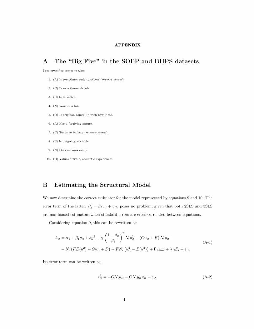
A The “Big Five” in the SOEP and BHPS datasets
I see myself as someone who:
1. (A) Is sometimes rude to others (reverse-scored).
2. (C) Does a thorough job.
3. (E) Is talkative.
4. (N) Worries a lot.
5. (O) Is original, comes up with new ideas.
6. (A) Has a forgiving nature.
7. (C) Tends to be lazy (reverse-scored).
8. (E) Is outgoing, sociable.
9. (N) Gets nervous easily.
10. (O) Values artistic, aesthetic experiences.
B Estimating the Structural Model
We now determine the correct estimator for the model represented by equations 9 and 10. The
error term of the latter, εyit = β2vit + uit, poses no problem, given that both 2SLS and 3SLS
are non-biased estimators when standard errors are cross-correlated between equations.
Considering equation 9, this can be rewritten as:
hit = α1 + β1yit + δy2it − γ(
1− β2β2
)2
Niy2it − (Cuit +B)Niyit+
−Ni(FE(u2) +Guit +D
)+ FNi
(u2it − E(u2)
)+ Γ1zhit + λEEi + eit.
(A-1)
Its error term can be written as:
εhit = −GNiuit − CNiyituit + eit. (A-2)
1

Given equation 3, yit and uit are correlated by construction. Substituting 10 in A-2, we
obtain:
εhit =−GNiuit − CNi(A2 +B2yit−1 + C2zait+
D2θai + β2vit + uit)uit + FNi(u2it − E(u2)
)+ eit.
(A-3)
from which we note that
E(εhit)− CNiE(u2) = 0. (A-4)
Therefore, we define εhit = εhit + CNiE(u2) and we rewrite equation A-1, as:
hit = α1 + β1yit + δy2it − γ(
1− β2β2
)2
Niy2it −BNiyit+
−Ni((F + C)E(u2) +D
)+ Γ1zhit + λEEi + εhit,
(A-5)
whose errors satisfy the conditional mean condition: E(εhit|Ni, Ei, yit, zit) = 0.
More precisely:
B =(1− β2) (β2γ1 − 2α2γ2)
β22
C = −2 (1− β2) γ2β22
D = λN −α22γ2β22
− α2γ1β2
F = − γ2β22
G =β2γ1 − 2α2γ2
β22
.
2

Moreover, substituting equation 3 in equation 5 we have:
A2 = α2 + α0β2
B2 = β2η0
C2 = β2Γ0
D2 = β2Λ0.
3

Table A.1: Income, Job Motivation and Personality Traits in Germany. 3SLS estima-tion; dependent variable is household income (standard errors in brackets).
Germany Germany Germany Germany2004 2004 2004 2004b/se b/se b/se b/se
IncomeSuccess Important 1.453*** 0.190* 2.616*** 0.193***
(0.114) (0.110) (0.144) (0.064)Education 0.162*** 0.115***
(0.006) (0.008)Age 0.113*** 0.058*** 0.056*** 0.029***
(0.010) (0.009) (0.013) (0.006)Age2 –0.001*** –0.001*** –0.000 –0.000***
(0.000) (0.000) (0.000) (0.000)Male –0.121** 0.146*** –0.429*** 0.010
(0.047) (0.043) (0.058) (0.026)Income at t−1 0.810***
(0.005)Success importantEducation 0.034*** 0.017*** –0.008*** 0.019***
(0.002) (0.002) (0.002) (0.002)Age –0.007** –0.000 –0.007** –0.000
(0.003) (0.003) (0.003) (0.003)Age2 –0.000*** –0.000*** –0.000*** –0.000***
(0.000) (0.000) (0.000) (0.000)Male 0.246*** 0.268*** 0.224*** 0.268***
(0.012) (0.013) (0.013) (0.013)Neuroticism –0.114*** 0.049 –0.001 0.041
(0.040) (0.044) (0.033) (0.044)Extraversion 0.270*** 0.285*** 0.163*** 0.286***
(0.045) (0.049) (0.037) (0.050)Conscientiousness 0.773*** 1.016*** 0.542*** 1.028***
(0.058) (0.061) (0.053) (0.063)Agreeableness –0.240*** –0.124** –0.108*** –0.136**
(0.051) (0.056) (0.042) (0.057)Openness 0.499*** 0.526*** 0.265*** 0.510***
(0.043) (0.047) (0.037) (0.048)Income at t−1 0.155***
(0.002)
N 13615 13615 12996 12996
4

Figure A.1: Life Satisfaction Distribution in the UK and Germany. Data in Per-centage of All Responses.
Figure A.2: Household Income distribution. UK and Germany. Income in 10K 2005USD.
5