A

porm©

K

1

tiotmoHf

ε

wne

η

b

0d

Electrochimica Acta 52 (2007) 3493–3504

Life of the Tafel equation: Current understanding andprospects for the second century

Oleg A. Petrii a,1, Renat R. Nazmutdinov b,1, Michael D. Bronshtein b, Galina A. Tsirlina a,∗,1

a Moscow State University, Chemical Faculty, 119992 Moscow, Russiab Kazan State Technological University, 420015 Kazan, Republic Tatarstan, Russia

Received 14 April 2006; received in revised form 4 October 2006; accepted 5 October 2006Available online 28 November 2006

bstract

The life of Tafel equation is considered briefly as evolution in the understanding of Tafel’s empiric parameters in the framework of varioushenomenological and theoretical approaches. Modern theories of the interfacial charge transfer reactions are employed to explain the behavior

f transfer coefficient versus electrode overvoltage and deviations of this quantity from 0.5 at low overvoltage. The effects of intramoleculareorganization, orbital overlap, reactant quantum modes and solvent dynamics are addressed and illustrated by model calculations. An attempt isade to propose new explanations of some data reported in the literature.2006 Elsevier Ltd. All rights reserved.

izatio

η

pWmpnetg

bStsare

eywords: Heterogeneous electron and proton transfer; Intramolecular reorgan

. Introduction

The famous paper of Tafel [1] started the epoch of quantita-ive approaches to electrode kinetics. An important idea stressedn Tafel’s paper is considering the current density dependencen overvoltage (not on the “absolute potential” or “decomposi-ion potential”). The values of hydrogen overvoltage for various

etals were reported for the first time. The linear dependencesf current density logarithm on overvoltage were presented forg, Pb and Cd. These empiric dependences were generalized as

ollows:

= a + b logJ, (1)

here overvoltage is ε, and the current density is J. The modernotations substituted ε for η and J for i, but never touched thempiric constants a and b:

= a + b logi. (2)

Eq. (2) can be most usually found now in the competent text-ooks (see, e.g. ref. [2]) and papers. The data presentation in

∗ Corresponding author. Tel.: +7 495 9391321; fax: +7 495 9328846.E-mail address: tsir@elch.chem.msu.ru (G.A. Tsirlina).

1 ISE member.

ciiht

013-4686/$ – see front matter © 2006 Elsevier Ltd. All rights reserved.oi:10.1016/j.electacta.2006.10.014

n; Solvent dynamics; Hydronium ion; Transfer coefficient

, log i coordinates became a conventional procedure, and peo-le employ this approach to study various reaction mechanisms.hen doing so they turn a little attention on the nature of ele-entary act. One can find the terms like “mass transfer Tafel

lot”, “ohmic Tafel plot” and “back reaction Tafel plot”, havingo relation to the elementary act of charge transfer. The consid-ration given below is restricted to the Tafel plots correspondingo the charger transfer reaction steps2 the most advanced branchrowing at the great tree of “Tafel Law”.

A century of the Tafel equation was noticed and markedy a number of papers, including the Special Issue of Corros.ci. prefaced by Burstein”s inspired essay [3]. We would like

o contribute to the jubilee celebrations by our current under-tanding of the physical reasons of Tafel’s experimental findingnd the essence of empiric parameters introduced in ref. [1]. Toeach this goal we need to trace the development of Tafel-likequations and to fix the most weak links in their experimentalonfirmation. We shall try to demonstrate that a number of exper-mental facts considered as contradicting can find explanation

n frames of molecular modeling of the charge transfer. Tafelad been at the head of an endless column of people looking forools and principles to control the rate of electrode reactions by

2 Here and below, we discuss exclusively the heterogeneous charge transfer.

3 imica

me

2

coeasLdlkptut

pidHpb

(

(

peith

spbasttagspip

boadhrlittbw

iaToadai

es1isst

reproduced in the textbooks as the illustration of good linear-ity of the typical semilogarithmic polarization curves. Whenreconsidering the collected curves in respect to mechanistic

3 For a low overvoltage (current) region, the contribution of impurity depo-larizers is significant, whereas for a high overvoltage (currents) interval themeasurements are strongly complicated by the ohmic drop. Rather complex(and usually uncertain) correction procedures are required for these both utmost

494 O.A. Petrii et al. / Electroch

eans of potential. This approach remains a key problem in thelectrode kinetics.

. Selection of experimental data for verification

Like any quantitative relation, the Tafel’s equation requires alear comprehension of the limits of its applicability. The choicef this limits should be understood from both theoretical andxperimental sides. The simplest but evidently unsatisfactorypproach from the experimental side is to consider any for linearemilogarithmic polarization curve as the confirmation of Tafelaw. More balanced approach assumes first of all the analysis ofeviations from linearity, i.e. from the Tafel-like behavior. Fol-owing the tradition and practice of XX century electrochemicalinetics, we do not separate the electron and proton transferrocesses in this consideration, and this approach does not con-radict the essence of our further logical steps because of theniversal nature of the basic theoretical approaches to variousypes of charge transfer.

Our consideration unwittingly intersects with the discussionresented recently by Gileadi and Kirowa-Eisner [4]. We acceptn general the tacit assumptions under which Eq. (2) should beiscussed for any charge transfer process, as listed in ref. [4].owever, looking through examples of the constant Tafel slopesresented in ref. [4] we easily notice that two assumptions shoulde formulated in a sharper manner.

1) Assumption (e) in ref. [4] looks as follows: “It is assumedthat only one reaction takes place in the region of poten-tial considered”. We prefer to reformulate it: “It is assumedthat there are no parallel reaction pathways, and the ratedetermining step is presented by the charge transfer processwith the participation of reactant having a fixed bulk con-centration, not an intermediate specie”. This reformulationis necessary to avoid the appearance of non-linearity or, viceversa, false linearity because of some reasons going fromthe formal kinetics of complex processes.

2) Assumption (f) in ref. [4] states: “The diffuse double layeris suppressed by a large excess of supporting electrolyteand/or a suitable correction is applied”. The uncertainty of‘suitable correction’ makes this point rather questionable. Inaddition, the diffuse layer effects are not exclusive becausea great number of reactions can be complicated by spe-cific adsorption and various local electrostatic interactions.We do not prefer to fix any certain correction as suitable,and suggest to check possible deviations from the Tafel-likebehavior under various assumptions regarding electrostaticeffects. Another formulation of this point is to check howrealistic is correction resulting in the Tafel-like behavior ofpolarization curve.

Point (1) is related to the problem of a complex reactionathway. One ought to mention that Tafel’s name is known in

lectrochemistry not only due to his famous equation, but alson relation to hydrogen reaction pathway, due to his idea abouthe recombination step. It was Tafel who initially attributedis polarization curves on Hg and Hg-like metals (with the

sitoa

Acta 52 (2007) 3493–3504

lope b = 0.107 V at 12 ◦C) to recombination step. This inter-retation had met immediately a number of objections mostlyecause of its inability to explain the value of dη/d(log j) slopend temperature dependence of this quantity (later also on theolution composition [5]). There are two “hydrogen” aspects ofhe Tafel equation: the reconsideration of recombination stepaking into account the potential dependence of surface cover-ge by hydrogen adatoms [6,7], and a search for some physicalrounds of the Tafel-like behavior for the hydronium dischargetep. Just the latter aspect finds itself far beyond the particularroblems of hydrogen evolution and appears to be extremelymportant for general consideration of the charge transferrocesses.

The elementary act of the discharge of a hydronium ion cane discussed in terms of the electron and proton transfer. The ratef this first order reaction can be measured directly on mercurynd some mercury-like metals. For these metals the hydroniumischarge is the first and simultaneously the limiting step ofydrogen evolution [5]. There is a uniquely wide overvoltageange for mercury (ca. 0.2–1.6 V) usually discussed as a purelyinear semilogarithmic curve. For example, such a representations given in the frequently cited paper [8]. More detailed informa-ion can be found in the famous monograph [9], it demonstrateshat the region under discussion is composed of a separate num-er of linear plots (each for the overvoltage region of 0.3–0.5 Vidth) obtained by different authors.The collection presented in ref. [9] contains the data obtained

n less dilute solutions in the absence of pronounced specificdsorption, therefore, it satisfies the criteria (2) discussed above.he slopes are really very close, but all segments do not fall intone straight line. Moreover, the regions of the lowest (0.2–0.4 V)nd the highest (1.3–1.6 V) overvoltage are presented by theata obtained under serious experimental complications,3 whilemid region (0.4–1.3 V) corresponds to more or less coincident

ndependent data.We can conclude that true experimental evidence of the lin-

ar semilogarithmic polarization curve for hydronium dischargetep is available only for ca. 1 V width region (η from 0.4 to.3 V). According to our knowledge, so wide linear Tafel regions unique [7], and no similar linearity was ever observed for anyimple charge transfer process. Such a sharp statement requirespecial comments concerning some data presented in the litera-ure.

A set of linear curves collected in Fig. 2 of ref. [8] is widely

ituations (see in ref. [6], for example); hence, the reliability of the slope values lower as compared to the slope in mid region. It is easy to see directly fromhe deviations of some points well reproduced in ref. [9]. Our thorough studyf the accuracy as reported in the original papers lead us to conclusion that thisccuracy is surely lower than for the mid overvoltage region.

imica

coah

3p

olacaecVeco

η

s

ctnBe

i

Bttbnst

gatafmcrNdc[

fi

pt

a

sefc

fitc

4

eGcwpiscarivsa

caibtTn

O.A. Petrii et al. / Electroch

omplications4 one can conclude that there is no exact evidencef the possibility to use any of reactions mentioned in ref. [8] asmodel reaction for consideration of Tafel’s law (excluding theydrogen evolution).

. Tafel’s equation retranslated by the earlyhenomenological theories of charge transfer

The consideration of charge (electron) transfer as a slow stepf complex electrode reactions, looking so natural and doubt-ess now, had been rather disputable for a long time. The initialttempts to give a semiquantitative treatment of the slow dis-harge step are associated with Audubert [12] and Butler [13]nd based on the ‘kinetic’ derivation of Nernst equation. Thexact formulation and mathematical presentation of slow dis-harge had been given in the classical paper by Erdey-Gruz andolmer [14]. Assuming the effect of potential on the activationnergy of electron transfer, the authors introduced the transferoefficient α as a parameter, and for a region of the moderatevervoltage η the Tafel equation written in the form:

= constant +(

RT

αF

)ln i. (3)

When α = 0.5, this equation gives a correct value for the Tafellope and describes its temperature dependence.

Frumkin [15] was the first to explain the experimentalurrent–overvoltage behavior by extending the Broensted rela-ion [16] (considering the hydronium discharge as a sort ofeutralization reaction). An important step had been done byutler [17], who introduced (without using this term),5 thexchange current density i0:

= i0

{exp

[αnFη

RT

]− exp

[− (1 − α)nFη

RT

]}. (4)

According to the famous textbook [19], Eq. (4) is referred toutler–Volmer equation (it is difficult to say who introduced for

he first time this frequently used double name). The number ofransferred electrons n should not be mixed with the total num-

er of electrons transferred in a multistep process; it denotes theumber of electrons transferred in a single slow electrochemicaltep, so typically n = 1. For the relatively high η values, Eq. (4)akes a form of the original Tafel equation, and its both empiric

4 Electrochemical transformations of benzene and nitrate, as well as the oxy-en evolution should be excluded from our consideration, as all these processesre electrocatalytic (with complex pathways), and there is no exact evidence forhe charge transfer as a limiting step in the overall overvoltage region. We alsovoid to consider both metallic Cu in solid electrolyte (too complex correctionor the mass transport limitations), and the curve for hexacyanoferreate (it waseasured [10] on a passive iron electrode in alkaline solution, and the surface

omposition could hardly remain unchanged in a wide potential range). The lasteaction from this collection is the oxidation of Cr(II) aquacomplex on mercury.o graph for this reaction is presented in the original paper [11]; the slope repro-uced in ref. [8] differs from the original slope given in ref. [11]; in addition, theomplications induced by the lability of water molecules in the aquacomplex11] are ignored.5 The notion of the exchange current density was clearly formulated for therst time by Dolin et al. [18].

cD

pctpetoeecT

fiao

Acta 52 (2007) 3493–3504 3495

arameters can be treated in terms of the phenomenologicalheory of charge transfer:

= − RT

αnFlni0; b = 2.3RT

αnF, (5)

till without any clear ideas how to explain and/or predict theffects of solution composition, as no any dependences of trans-er coefficient and exchange current density on the nature andoncentration of supporting electrolyte were expected.

We discuss i0 and α parameters instead of a and b, as under therst approximation they represent the overvoltage-independent

erm and d(log i)/dη (note that if α depends on overvoltage, theonstant a is already overvoltage-dependent).

. Towards the elementary act and molecular features

The important physical features of electron transfer (ET) inlectrochemical systems had been noticed for the first time byurney in his paper [20] truly appreciated after a long delay. In

ontrast, the model proposed later by Horiuti and Polanyi [21]as rapidly accepted. A general idea to construct the curves ofotential energy for reactant and product still remains a key tooln the theory of elementary act. The main result of these earlytudies appeared to be physical interpretation of the transferoefficient α, or, in other words, a sort of physical substanti-tion of the Broensted-like empiric relations. However, it stillemained unclear: (i) why α ≈ 0.5 for hydronium discharge (ast followed from the Tafel slope value b); (ii) whether α �= 0.5alues are possible for other reactions; (iii) why α remains con-tant in a certain overvoltage interval. No progress was achievedlso in understanding the effects of solution composition.

The latter aspect was clarified by Frumkin in his slow dis-harge theory [22], still based on Broensted equation, but withllowance for more realistic potential distribution in the vicin-ty of charged interfaces. The treatment of experimental dataased on Frumkin theory (widely known as Frumkin correc-ion) eliminates the potential-dependent double layer effects.his procedure consists of two steps [23], namely (1) determi-ation of the mean reactant charge in the solution bulk and (2)onstruction of the corrected Tafel plots introduced initially byelahay and co-workers [24].The slow discharge theory offered a principle way for a more

recise determination of the transfer coefficients and exchangeurrent densities (rate constants) by fixing the relations betweenrue (corrected) and experimental (apparent) values of thesearameters. In 1960–1970s, Frumkin school provided a strongxperimental contribution to the double layer effects in elec-rochemical kinetics, especially due to the lucky experimentalbservation of anions electroreduction at negatively chargedlectrodes [23,25]. The latter situation amplifies the effect oflectrostatic repulsion of the reactant and allows to observe thehange not only in the value, but also in the sign of an apparentafel’s parameter b.

To summarize, one should consider Frumkin theory as therst physically grounded theory in electrochemical kinetics,s it operates with a less phenomenological parameter namedriginally the mean potential in the plane of reactant localiza-

3 imica

trufccp

trtetMrhfcspba

taLa

γ

wλ

ft

air

α

ca

j

wFf

te

(

eMa

α

wctcssae

b

((

(

(

(

t

496 O.A. Petrii et al. / Electroch

ion [22] (later “psi-prime potential” [23,25]). The electrostaticeactant–electrode interactions can be now considered at molec-lar level [26–28], and can be also more precisely extractedrom experimental data [29]. A bottleneck of the slow dis-harge theory is not so much the uncertainty of its electrostaticomponent,6 but first of all the phenomenological nature of otherarameters (rate constant and transfer coefficient).

The next level of understanding became available due toheoretical findings by Marcus [30] and Levich (see earlyeview [31]). Unfortunately it took a long time to ‘translate’heir equations into the language accepted by experimentallectrochemists, but finally the transfer coefficient α (and simul-aneously Tafel parameter b) acquired transparent interpretation.

odern theoretical approaches never rejected the Broenstedelation, but enabled to clarify its physical reasons and explainedow this famous relation should be applied in less straight-orward manner (‘microscopic’ Broensted relation, remainingorrect at any fixed overvoltage, but without obligatory con-tancy of the transfer coefficient). The importance of thisroblem for chemical kinetics can be hardly overestimatedecause of the multiplicity of reactions involving proton transfers the elementary step [32].

A variety of the ET processes occurring at an elec-rode/solution interface can be roughly divided into adiabaticnd diabatic reactions. Usually, one needs an estimate of theanday–Zener factor (γe) to judge directly about the reactiondiabacity [31,33]. For low overvoltages,

e ≈ ρ(εF )kT

(hωeff)2

√πkT

λ

(Ee

2

)2

. (6)

here ρ(εF) is the density of electronic states at the Fermi level,the total reorganization energy, ωeff the effective frequency

actor (≈1013 s−1) and Ee is the resonance splitting of reactionerms in the crossing point.7

According to the Marcus theory developed initially for adi-batic reactions (γe � 1) the transfer coefficient can be writtenn a simple form as a function of the overvoltage and totaleorganization energy:

= 1

2− Fη

2λ. (7)

For the diabatic limit of the electron transfer (γe � 1) the totalurrent can be estimated by integrating over the energy levels ofmetal electrode ε [31,33]:

≈∫ +∞

−∞ρ(ε)n(ε) exp

[− (λ − ε − Fη)2

4λkT

]dε, (8)

here ρ(ε) is the density of electronic states and n(ε) is theermi–Dirac distribution function (the Fermi level is reckonedrom zero).

6 We will use further only the corrected values of experimentally determinedransfer coefficients from authoritative sources, or the values obtained with highnough electrolyte concentrations.7 If the electron transfer is accompanied by the bond break, the factor before

Ee/2)2 should be modified.

Acta 52 (2007) 3493–3504

The integration plays a crucial role when considering the highlectrode overvoltages and excludes the appearance of invertedarcus region (observed for homogeneous ET reactions). The

nalysis of Eq. (8) (see ref. [34]) allows to define α in the form:

≈ 1 − n(ε∗), (9)

here ε* is the effective energy level which gives the largestontribution to the resulting current. If ε* lies significantly lowerhan the Fermi level, the α values tend to zero (activationless dis-harge). Thus, Eqs. (8) and (9) stress the importance of electronictructure of a metal electrode for the diabatic ET. It should betressed that these findings are valid for the combined electronnd proton transfer (in part, for the electrochemical hydrogenvolution).

It is easy to see that Eqs. (7) and (9) predict the followingehavior of transfer coefficient:

1) α = 0.5 for zero overvoltage;2) linear decrease of α with overvoltage in the normal Marcus

region;3) asymptotic decrease of α with overvoltage in the vicinity of

the activationless region;4) possibility of the apparent independence of α on overvoltage

in a relatively narrow overvoltage interval;5) impossibility of the non-monotonous α versus η behavior.

Let us list the initial observations stimulating us to considerhe problem more systematically.

Prediction (1).A typical error in α usually exceeds ±0.02, being even

higher for more dilute solutions. One can consider, therefore,the reported values of 0.45–0.55 as agreement with prediction(1). Bearing in mind the maximal possible experimental erroraffected the α values one can conclude (see Eq. (8)) that α

remains overvoltage-independent in the interval of ∼0.05λ/Fwidth, i.e. at ∼0.05λ/F V this quantity is expected to remainclose to 0.5. At the same time, there are many examples of thetransfer coefficient falling beyond 0.45–0.55 limits at alreadyvery low overvoltage of 50–150 mV [11,35,36], despite thevalues of λ are high enough (above 200 kJ mol−1).Predictions (2) and (3).

A linear decrease of α with overvoltage for a number oforganic reactants was studied systematically by the Saveantand Tessier [37,38], and Eq. (7) was confirmed for a num-ber of systems (see ref. [26] for a brief review of the otherdata of this sort). Typically the diffusion limitations compli-cate such experiments at high overvoltage, but an exceptionalpossibility to penetrate into this region appears under strongelectrostatic repulsion (electroreduction of anions). These reac-tions can be studied at the boundary of the normal Marcusregion and beyond, providing the experimental confirmation

[39] of Eq. (9).Prediction (4)

For the hydrogen evolution on mercury, the experimentalregion of Tafel behavior is of 1.2 V and the reaction formally

imica Acta 52 (2007) 3493–3504 3497

4

(rte

U

a

U

wcaftrs

gtc“msjoul

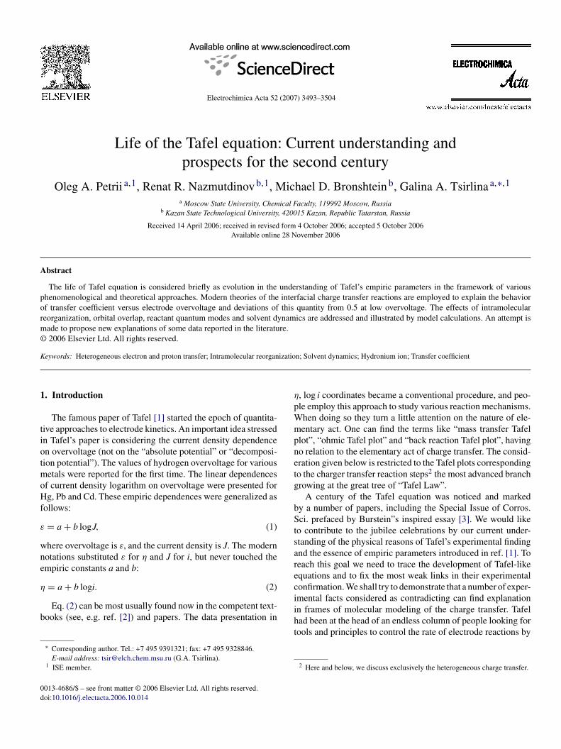
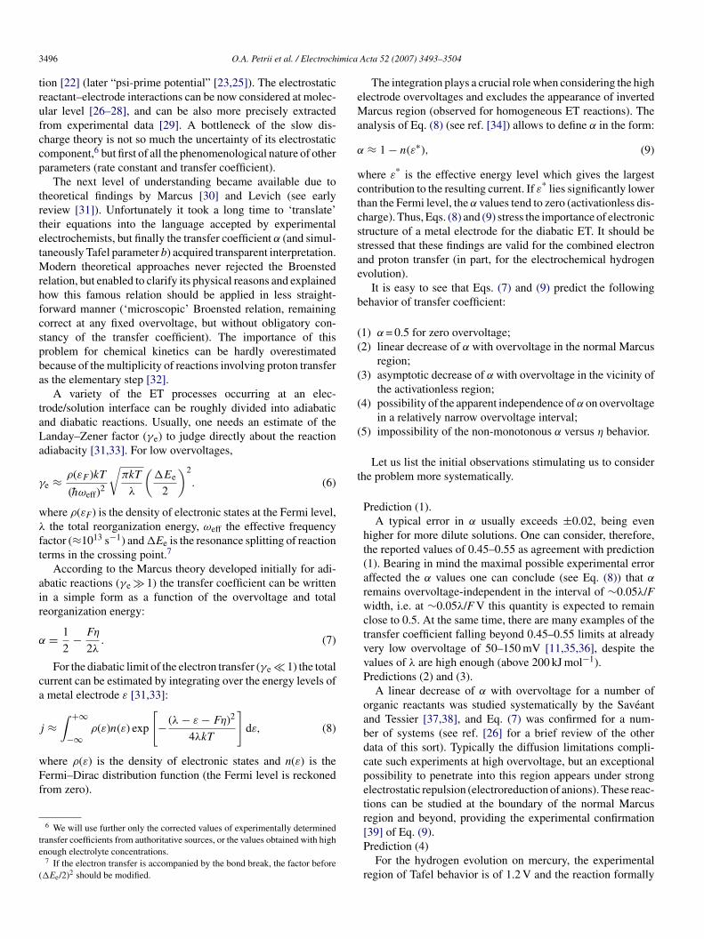
Fig. 1. The fragment of the free energy surface describing the ET with the asym-mη

mnaKto

adtν

f

α

i

α

a

gca

O.A. Petrii et al. / Electroch

satisfies Eq. (8) at λ ≈ 2 MJ mol−1. This value can hardly beregarded as physically reasonable being at least an order higherthan any possible estimate of the solvent and innersphere reor-ganization energies.Prediction (5)

A non-monotonous α versus η behavior was reported bythe Maran’s group for a number of organic reactants [40–42]when reduction was accompanied by the bond rupture. For thistype of electron transfer reaction, a wide-spread theoreticaltreatment of α is based on the Saveant’s model of so-calledconcerted electron transfer [43,44]. This simplified treatmentpresents a limiting case of a more general theory of the bondbreaking electron transfer (BBET) (see, e.g. ref. [45]).

Our main goal is to consider systematically the basic phys-ical reasons inducing deviations from the Marcus predictionsregarding the α behavior, as well as the models/theories whichcan be additionally employed. An important aspect of the prob-lem is working out a qualitative diagnostic approach for theinitial choice of a suitable model, as no direct experimentalobservations can discover a certain type of the elementary act.

In subsequent sections we address the effects of inner-spherereorganization, electrode–reactant coupling, quantum modesof reactant and solvent dynamics on the behavior of α versusη. For the sake of simplicity we restrict ourselves to the one-stepelectron transfer.

.1. Effects of intramolecular reorganization

Let us consider first the diabatic free energy surfaces for initiali) and final (f) states. If both the solvent and intramoleculareorganization can be described in terms of the linear responseheory [33], the energy surfaces are parabolic and the relevantquations take the form:

i(q, qin) = λsq2 + λinq

2in, (10)

nd

f(q, qin) = λs(q − 1)2 + �λin(qin − 1)2 − Fη,

here q and qin are the dimensionless solvent and intramolecularoordinates, respectively, λs is the solvent reorganization energynd λin and �λin refer to the intramolecular reorganization energyor reduction and oxidation, respectively. In general q can bereated as a fraction of the reactant charge which changes soapidly that the reactant interacts only with the fast modes ofolvent.

Eq. (10) addresses the “asymmetry” of inner-sphere reor-anization (λin �= �λin), which stems from a difference betweenhe classical vibration modes of reactant and product. A typi-al example of the adiabatic free energy surface comprising theasymmetry” effect is shown in Fig. 1. Note that for the sym-etry case (λin = �λin) the projection of saddle line is a straight

egment. On the contrary, if λin �= �λin, the corresponding pro-

ection is a parabolic curve (Fig. 1). Some results of calculationsf the ET kinetic parameters taking into account the intramolec-lar asymmetry have been reported earlier in refs. [46] (diabaticimit) and [47] (adiabatic ET). The problem of innersphere asym-

r0oo

etry of intramolecular reorganization (λs = 0.7 eV, λin = 1 eV, �λin = 0.3 eV,= 0 V). The initial state corresponds to (0,0), the final state corresponds to (1,1).

etry was mentioned by Schmickler [48], although the authoreglected this effect in the model calculations. The effect ofsymmetry of intramolecular reorganization was addressed byuznetsov and Ulstrup [49]. The authors built the model activa-

ion barrier versus the reaction free energy considering changef intramolecular vibrations going from reactant to product.

To calculate the activation energy as a function of overvolt-ge, one needs to find the saddle point of potential surfaceefined by Eq. (10). It is impossible to build any simple equa-ion for transfer coefficient for an arbitrary asymmetry factor,= �λin/λin. However, one can easily derive simple asymptotic

ormulas for two limiting cases. If ν � 1,

≈ 1

2

(1 +

�λin

λs

)− Fη

2λs, (11)

.e. the transfer coefficient exceeds 0.5 at zero overvoltage.For the opposite limit ν � 1,

≈ 1

2

(1 −

λin

λs

)− Fη

2λs, (12)

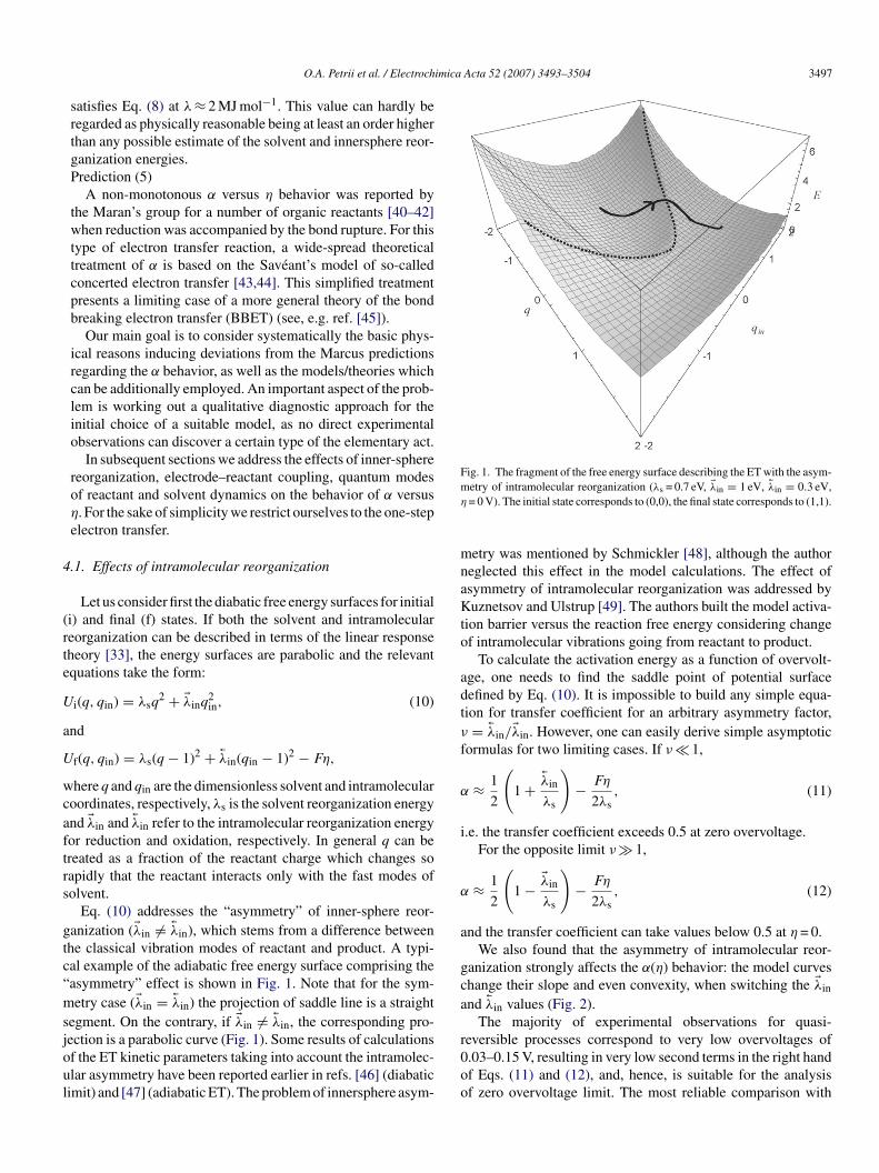
nd the transfer coefficient can take values below 0.5 at η = 0.We also found that the asymmetry of intramolecular reor-

anization strongly affects the α(η) behavior: the model curveshange their slope and even convexity, when switching the λin

nd �λin values (Fig. 2).The majority of experimental observations for quasi-

eversible processes correspond to very low overvoltages of.03–0.15 V, resulting in very low second terms in the right handf Eqs. (11) and (12), and, hence, is suitable for the analysisf zero overvoltage limit. The most reliable comparison with

3498 O.A. Petrii et al. / Electrochimica Acta 52 (2007) 3493–3504

Fig. 2. Transfer coefficient vs.ηdependencies illustrating the effects of asymme-tod

eEbo

bCtrtraa[mhadrsNtena

trnptf

U

a

U

Foc

ectdist

α

wui(t

α

w

(

1

2

3

ry of inner-sphere reorganization: λs = 0.7 eV, λin = 1 eV, �λin = 0.25 (squares)r 0.5 (circles) eV; λin = 1 eV, �λin = 0.25 (triangles up) or 0.5 (trianglesown) eV.

xperiment in terms of the α deviation from 0.5 can be done forq. (11): even if the second term is essential, its effect cannote mixed with the key effect of the first term because of thepposite signs.

Possible examples of the behavior predicted by Eq. (11) cane found for the reduction of [Co(en)3]3+ (α ∼ 0.8) [35] and ther(III) amino complexes (α ∼ 0.65–0.8) [36]. Since electron is

ransferred to the antibonding molecular orbital of the complexeactants, the innersphere reorganization can be noticeable (withhe asymmetry factor ν < 1). An opposite type of behaviour cor-esponding to Eq. (12) was reported for the reduction of V(III)quacomplexes [35]. The oxidation of Eu(II) aquacomplexeslso demonstrates a pronounced deviation from 0.5 (α ∼ 0.2)11] (it is evident that for the oxidation of a complex the asym-etry factor most likely >1). The quantitative comparison is

ardly possible in the framework of asymptotic formulas (11)nd (12), because for real systems neither ν � 1, nor ν � 1 con-itions are satisfied (see examples in ref. [46]). However, theatios of innersphere and solvent reorganisation energies respon-ible for the degree of α deviation from 0.5 can exceed unity.ote that a value of 0.6 for the transfer coefficient reported for

he electroreduction of [Ru(NH3)6]3+ [35] cannot be discussedven qualitatively using Eq. (11), as the intramolecular reorga-ization of the complex is very small (electron is transferred tobinding molecular orbital).

At a very strong intramolecular reorganization, the electronransfer results in the chemical bond rupture. Since the linearesponse theory can be used only to describe the solvent reorga-ization in such reactions, one needs to employ “non-parabolic”otentials Ui(f)(r) (r is the intramolecular coordinate) to handlehe reorganization of inner sphere. The equations for diabaticree energy surfaces look as follows:

(q, r) = λ q2 + U (r) (13)

i s i

nd

f(q, r) = λsq2 + Uf(r) − Fη.

tdt

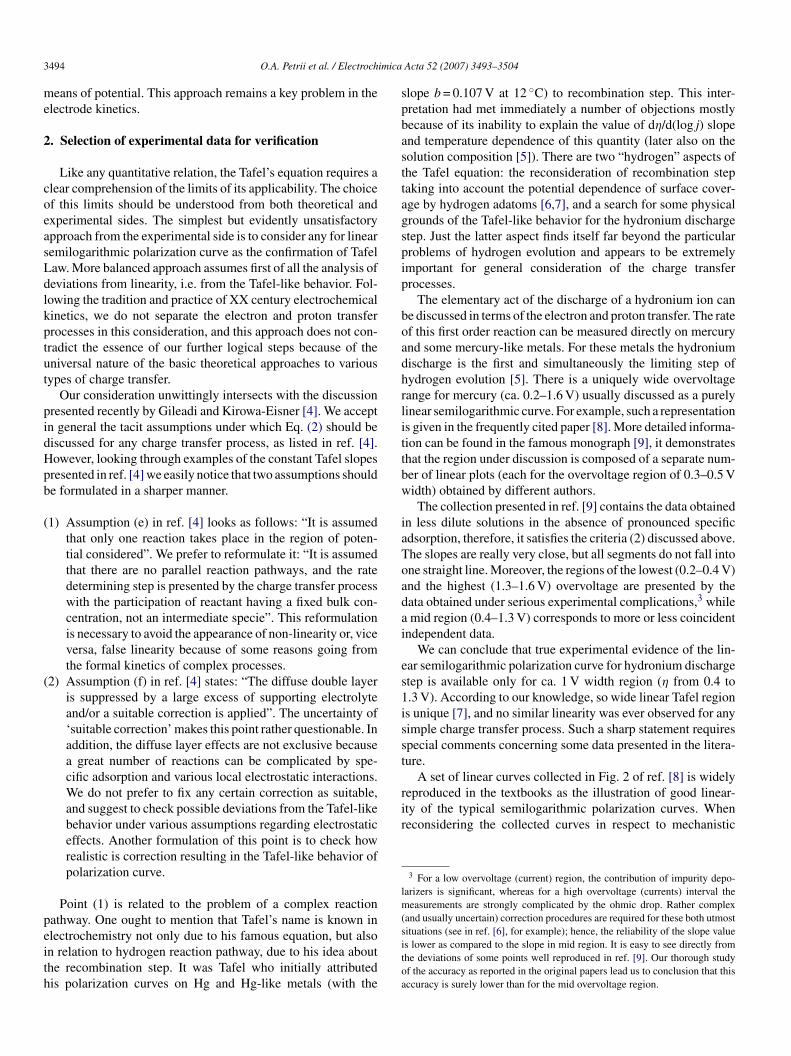
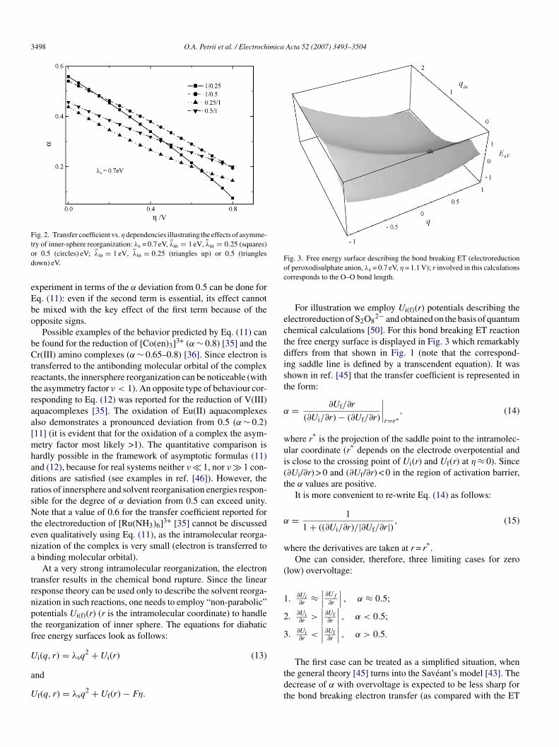
ig. 3. Free energy surface describing the bond breaking ET (electroreductionf peroxodisulphate anion, λs = 0.7 eV, η = 1.1 V); r involved in this calculationsorresponds to the O–O bond length.

For illustration we employ Ui(f)(r) potentials describing thelectroreduction of S2O8

2− and obtained on the basis of quantumhemical calculations [50]. For this bond breaking ET reactionhe free energy surface is displayed in Fig. 3 which remarkablyiffers from that shown in Fig. 1 (note that the correspond-ng saddle line is defined by a transcendent equation). It washown in ref. [45] that the transfer coefficient is represented inhe form:

= ∂Uf/∂r

(∂Ui/∂r) − (∂Uf/∂r)

∣∣∣∣r=r∗

, (14)

here r* is the projection of the saddle point to the intramolec-lar coordinate (r* depends on the electrode overpotential ands close to the crossing point of Ui(r) and Uf(r) at η ≈ 0). Since∂Ui/∂r) > 0 and (∂Uf/∂r) < 0 in the region of activation barrier,he α values are positive.

It is more convenient to re-write Eq. (14) as follows:

= 1

1 + ((∂Ui/∂r)/|∂Uf/∂r|) , (15)

here the derivatives are taken at r = r*.One can consider, therefore, three limiting cases for zero

low) overvoltage:

. ∂Ui

∂r≈∣∣∣ ∂Uf

∂r

∣∣∣ , α ≈ 0.5;

. ∂Ui∂r

>

∣∣∣ ∂Uf∂r

∣∣∣ , α < 0.5;

. ∂Ui∂r

<

∣∣∣ ∂Uf∂r

∣∣∣ , α > 0.5.

The first case can be treated as a simplified situation, whenhe general theory [45] turns into the Saveant’s model [43]. Theecrease of α with overvoltage is expected to be less sharp forhe bond breaking electron transfer (as compared with the ET

imica Acta 52 (2007) 3493–3504 3499

a

α

wop

rvcobtoaa

dlwpSOtat[twbad

isc

Fte

Fo0

4

sfcsttfatta

O.A. Petrii et al. / Electroch

ccompanied with a lower intramolecular reorganization) [43]:

= 1

2− Fη

(λs + D), (16)

here D is the bond rupture energy. This simple equation isbtained under assumption that the exponents of the repulsiveart of the Morse and decay terms are equal.

We believe that the numerous manifestations of low α

eported for organic reactants at potentials close to reversiblealue (see ref. [40]), for example, might be attributed to thease 2, being already beyond the Saveant’s model. The otherbservations (α > 0.5) for the same type of reactions [41] mighte explained in terms of the limiting case 3. A special computa-ional analysis is surely required in addition to systematic studiesf Saveant’s and Maran’s groups, to check the correctness of thebovementioned assumption and to judge about the necessity topply ‘beyond Saveant’ models.

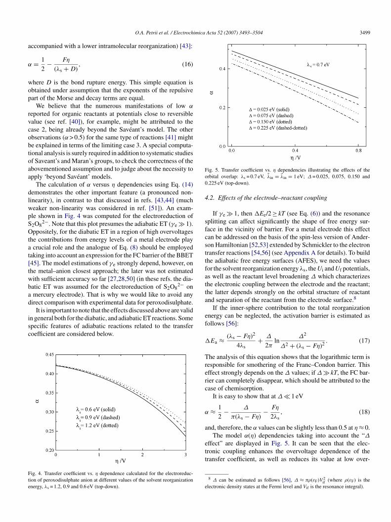
The calculation of α versus η dependencies using Eq. (14)emonstrates the other important feature (a pronounced non-inearity), in contrast to that discussed in refs. [43,44] (mucheaker non-linearity was considered in ref. [51]). An exam-le shown in Fig. 4 was computed for the electroreduction of2O8

2−. Note that this plot presumes the adiabatic ET (γe � 1).ppositely, for the diabatic ET in a region of high overvoltages

he contributions from energy levels of a metal electrode playcrucial role and the analogue of Eq. (8) should be employed

aking into account an expression for the FC barrier of the BBET45]. The model estimations of γe strongly depend, however, onhe metal–anion closest approach; the later was not estimatedith sufficient accuracy so far [27,28,50] (in these refs. the dia-atic ET was assumed for the electroreduction of S2O8

2− onmercury electrode). That is why we would like to avoid any

irect comparison with experimental data for peroxodisulphate.

It is important to note that the effects discussed above are valid

n general both for the diabatic, and adiabatic ET reactions. Somepecific features of adiabatic reactions related to the transferoefficient are considered below.

ig. 4. Transfer coefficient vs. η dependence calculated for the electroreduc-ion of peroxodisulphate anion at different values of the solvent reorganizationnergy, λs = 1.2, 0.9 and 0.6 eV (top-down).

ef

Trerc

α

a

ett

e

ig. 5. Transfer coefficient vs. η dependencies illustrating the effects of therbital overlap: λs = 0.7 eV, �λin = λin = 1 eV; Δ = 0.025, 0.075, 0.150 and.225 eV (top-down).

.2. Effects of the electrode–reactant coupling

If γe � 1, then Ee/2 ≥ kT (see Eq. (6)) and the resonanceplitting can affect significantly the shape of free energy sur-ace in the vicinity of barrier. For a metal electrode this effectan be addressed on the basis of the spin-less version of Ander-on Hamiltonian [52,53] extended by Schmickler to the electronransfer reactions [54,56] (see Appendix A for details). To buildhe adiabatic free energy surfaces (AFES), we need the valuesor the solvent reorganization energy λs, the Ui and Uf potentials,s well as the reactant level broadening Δ which characterizeshe electronic coupling between the electrode and the reactant;he latter depends strongly on the orbital structure of reactantnd separation of the reactant from the electrode surface.8

If the inner-sphere contribution to the total reorganizationnergy can be neglected, the activation barrier is estimated asollows [56]:

Ea ≈ (λs − Fη)2

4λs+ Δ

2πln

Δ2

Δ2 + (λs − Fη)2 . (17)

he analysis of this equation shows that the logarithmic term isesponsible for smothering of the Franc–Condon barrier. Thisffect strongly depends on the Δ values; if Δ � kT, the FC bar-ier can completely disappear, which should be attributed to thease of chemisorption.

It is easy to show that at Δ � 1 eV

≈ 1

2− Δ

π(λs − Fη)− Fη

2λs, (18)

nd, therefore, the α values can be slightly less than 0.5 at η ≈ 0.The model α(η) dependencies taking into account the “Δ

ffect” are displayed in Fig. 5. It can be seen that the elec-ronic coupling enhances the overvoltage dependence of theransfer coefficient, as well as reduces its value at low over-

8 Δ can be estimated as follows [56], Δ ≈ πρ(εF)V 2if (where ρ(εF) is the

lectronic density states at the Fermi level and Vif is the resonance integral).

3 imica

v(adeefoin

mHiα

te

5p

atc(cdfnwso

cicea

j

wv

eaioSbpo

t

j

w

tlo[

td(qttt

[cransthias

v[syvtt(to

500 O.A. Petrii et al. / Electroch

oltage. Since α can be slightly less than 0.5 even at η = 0 Vsee Eq. (18)), the experimental examples of this sort discussedbove should be considered mandatory under two indepen-ent assumptions (innersphere asymmetry and the couplingffect).9 Note that when α > 0.5 the second assumption can bexcluded. The influence of electronic coupling on the trans-er coefficient was explored first in ref. [58] using the modelf a surface molecule (linear combination of atomic orbitals)n the Hartree–Fock approximation. The author has reported aon-monotonous behaviour of α when increasing overpotential.

It should be stressed that both the solvent and intramolecularodes were treated as classical in all reactions considered above.owever, the quantum character of some modes of the reactant

nner sphere (hw > kT ) can affect considerably the behaviour of(η). This important effect will be discussed in the next section

aking the electrochemical discharge of H3O+ ion as a goodxample.

. Mystery of the hydrogen evolution on mercury:roton transfer

The discharge of a hydronium ion with formation of andsorbed intermediate (H3O+ + e → Hads + H2O) is well-knowno be the rate controlling step of the hydrogen evolution at a mer-ury electrode We combined the Dogonadze–Kuznetsov–LevichDKL) theory [31,59,60] with a quantum chemical approach tolarify some molecular aspects of this reaction. The detailediscussion of the model and computational approaches can beound ref. [61]. The motion of system along the solvent coordi-ate was treated as classical, while the quantum tunneling effectsere considered for the proton degree of freedom. The mercury

urface was modeled by a cluster; the nearest solvation sheathf hydronium ion was considered as well [61].

The total current j was calculated as a sum of the partialontributions jnm (corresponding to the proton transfer from annitial energy level n to a final state m) normalized to the statisti-al sum Z =∑n exp{−ε

(i)1n/kT }, where ε

(i)1n is the excitation

nergy of a proton from the ground level (1) in initial state (i) togiven vibration state (n):

= 1

Z

∑n,m

jnm. (19)

Since the electron transfer at the hydronium ion discharge

as found to be significantly adiabatic [61], we can employ theersion of DKL theory developed for a strong coupling between

9 When comparing any computational results for adiabatic reactions withxperiment, one should take special care of the experimental evidence ofdiabaticity. A complex interplay of dynamic and static solvent effects andmpossibility to change the solvent relaxation parameters without simultane-us change of its permittivity strongly complicate the experimental diagnostics.imultaneously, the absence of the observable dynamic solvent effect cannote considered as the evidence of non-adiabaticity, at least for reactions withronounced innersphere contribution to reorganization energy and/or for highvervoltage. The problem is discussed in detail in our recent paper [57].

p

cedpifTtah

Acta 52 (2007) 3493–3504

he ET diabatic states:

nm ≈ κ(nm)p exp

{−ε

(i)1n

kT

}

×exp

⎧⎨⎩− (λs + HH2

ads + ε(f)m − ε

(i)n − Fη)

2

4λskT

⎫⎬⎭ , (20)

here κ(nm)p is the partial proton transmission coefficients (the

unneling probability), ε(i)n and ε

(f)m the quantum vibration energy

evels in initial (i) and final (f) states and EH2dis.ads is the energy

f dissociative adsorption of a hydrogen molecule on mercury62].

The quantum chemical calculations at the DFT level predictwo-level potentials as a function of the proton–mercury clusteristance for several positions H3O+relative to the metal surface0.36 nm ≤ r(Hg–O) ≤ 0.44 nm) [61]. The proton vibration fre-uencies were found to be quantum in the both wells. Note thathe computational results do not support the key assumption ofhe Benderskii–Ovchinnikov’s model [63] (according to whichhe proton motion in the final state is treated as classical).

The model calculations were performed using a new approach61]. This approach allows to address (within a self-consistentomputational scheme) the non-equilibrium solvent effectsesponsible for the equalizing the proton energy levels in anrbitrary two-well potential. It should be stressed that the tun-eling probability of proton was found to depend crucially on theequence number of exited proton states. Being rather small forhe ground states, this quantity becomes exceedingly large forighly exited vibrational energy levels due to the sharp increas-ng of overlap between the proton wave functions. This enables

noticeable contribution from the vibrationally exited protontates to the Tafel plots.

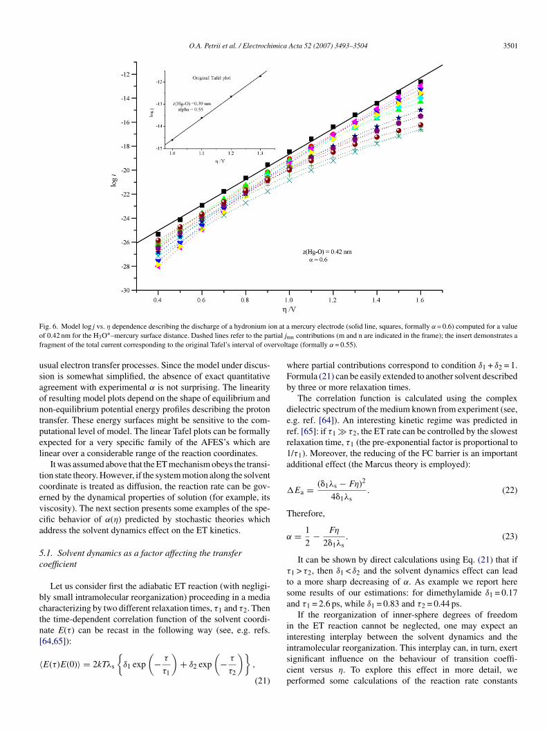
Fig. 6 presents an example of the resulting curve. The over-oltage interval is chosen in agreement with the collection in ref.9]. The quasi-linear behavior of the total current is observed inemilogarithmic coordinates (squared points, solid line), whichields a value of 0.6 for the effective transfer coefficient. Thisαeffalue demonstrates low sensitity to the mercury–hydronium dis-ance and solvent reorganization energy. However, if we excludehe region of low overvoltages and start regression from 0.8 Vthe most usual lower limit in experimental studies), αeff appearso be 0.53–0.55. The insert in Fig. 5 presents the imitation ofriginal Tafel’s data. For his narrow interval the linearization iserfect, with αeff = 0.55.

The dashed curves in Fig. 6 demonstrate the various partialontributions. It can be seen that any partial curve is less lin-ar as compared with the sum of all currents, i.e. our modeliscloses an important reason of the mysterious linearity: whenartial α starts to decrease with overvoltage (the ‘Marcus’ barriers assumed in Eq. (19) for jnm), a compensating effect appearsrom contribution of another proton level. Thus, the origin of the

afel plots can be ascribed mostly to the interplay between con-

ributions from the different proton energy levels. This simplend physically transparent reason is most likely specific for theydronium ion discharge and cannot be expected, in general, for

O.A. Petrii et al. / Electrochimica Acta 52 (2007) 3493–3504 3501

F n at ao rtial jmf ervolt

usaontpel

tcevca

5c

bctn[

〈

wFb

derr1a

T

α

τ

tsa

ii

ig. 6. Model log j vs. η dependence describing the discharge of a hydronium iof 0.42 nm for the H3O+–mercury surface distance. Dashed lines refer to the paragment of the total current corresponding to the original Tafel’s interval of ov

sual electron transfer processes. Since the model under discus-ion is somewhat simplified, the absence of exact quantitativegreement with experimental α is not surprising. The linearityf resulting model plots depend on the shape of equilibrium andon-equilibrium potential energy profiles describing the protonransfer. These energy surfaces might be sensitive to the com-utational level of model. The linear Tafel plots can be formallyxpected for a very specific family of the AFES’s which areinear over a considerable range of the reaction coordinates.

It was assumed above that the ET mechanism obeys the transi-ion state theory. However, if the system motion along the solventoordinate is treated as diffusion, the reaction rate can be gov-rned by the dynamical properties of solution (for example, itsiscosity). The next section presents some examples of the spe-ific behavior of α(η) predicted by stochastic theories whichddress the solvent dynamics effect on the ET kinetics.

.1. Solvent dynamics as a factor affecting the transferoefficient

Let us consider first the adiabatic ET reaction (with negligi-ly small intramolecular reorganization) proceeding in a mediaharacterizing by two different relaxation times, τ1 and τ2. Thenhe time-dependent correlation function of the solvent coordi-ate E(τ) can be recast in the following way (see, e.g. refs.

64,65]):

E(τ)E(0)〉 = 2kTλs

{δ1 exp

(− τ

τ1

)+ δ2 exp

(− τ

τ2

)},

(21)

iscp

mercury electrode (solid line, squares, formally α = 0.6) computed for a value

n contributions (m and n are indicated in the frame); the insert demonstrates aage (formally α = 0.55).

here partial contributions correspond to condition δ1 + δ2 = 1.ormula (21) can be easily extended to another solvent describedy three or more relaxation times.

The correlation function is calculated using the complexielectric spectrum of the medium known from experiment (see,.g. ref. [64]). An interesting kinetic regime was predicted inef. [65]: if τ1 � τ2, the ET rate can be controlled by the slowestelaxation time, τ1 (the pre-exponential factor is proportional to/τ1). Moreover, the reducing of the FC barrier is an importantdditional effect (the Marcus theory is employed):

Ea = (�1λs − Fη)2

4�1λs. (22)

herefore,

= 1

2− Fη

2�1λs. (23)

It can be shown by direct calculations using Eq. (21) that if1 > τ2, then δ1 < δ2 and the solvent dynamics effect can leado a more sharp decreasing of α. As example we report hereome results of our estimations: for dimethylamide δ1 = 0.17nd τ1 = 2.6 ps, while δ1 = 0.83 and τ2 = 0.44 ps.

If the reorganization of inner-sphere degrees of freedomn the ET reaction cannot be neglected, one may expect annteresting interplay between the solvent dynamics and the

ntramolecular reorganization. This interplay can, in turn, exertignificant influence on the behaviour of transition coeffi-ient versus η. To explore this effect in more detail, weerformed some calculations of the reaction rate constants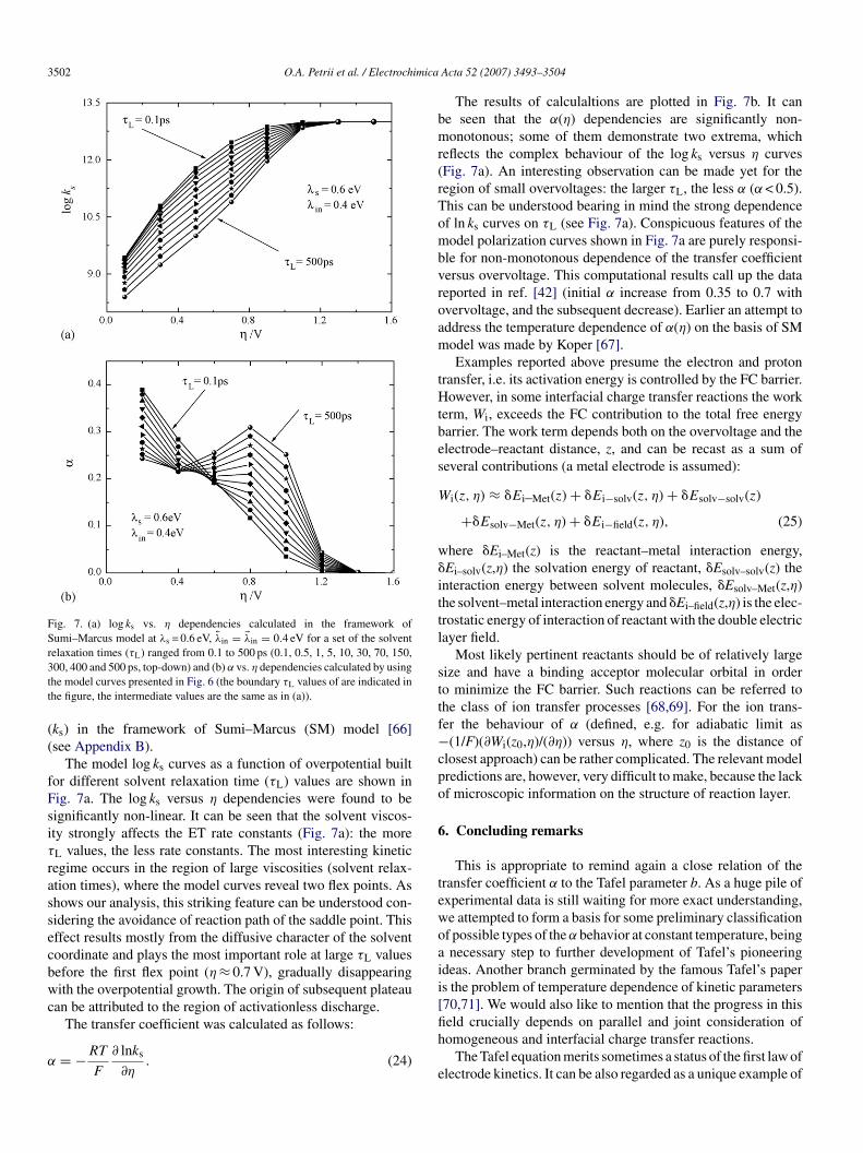

3502 O.A. Petrii et al. / Electrochimica

Fig. 7. (a) log ks vs. η dependencies calculated in the framework ofSumi–Marcus model at λs = 0.6 eV, �λin = λin = 0.4 eV for a set of the solventrelaxation times (τ ) ranged from 0.1 to 500 ps (0.1, 0.5, 1, 5, 10, 30, 70, 150,3tt

((

fFsiτ

rassecbwc

α

bmr(rTombvroam

tHtbes

W

w�ittl

sttf−cpo

6

tewoaii[

L

00, 400 and 500 ps, top-down) and (b) α vs. η dependencies calculated by usinghe model curves presented in Fig. 6 (the boundary τL values of are indicated inhe figure, the intermediate values are the same as in (a)).

ks) in the framework of Sumi–Marcus (SM) model [66]see Appendix B).

The model log ks curves as a function of overpotential builtor different solvent relaxation time (τL) values are shown inig. 7a. The log ks versus η dependencies were found to beignificantly non-linear. It can be seen that the solvent viscos-ty strongly affects the ET rate constants (Fig. 7a): the moreL values, the less rate constants. The most interesting kineticegime occurs in the region of large viscosities (solvent relax-tion times), where the model curves reveal two flex points. Ashows our analysis, this striking feature can be understood con-idering the avoidance of reaction path of the saddle point. Thisffect results mostly from the diffusive character of the solventoordinate and plays the most important role at large τL valuesefore the first flex point (η ≈ 0.7 V), gradually disappearingith the overpotential growth. The origin of subsequent plateau

an be attributed to the region of activationless discharge.

The transfer coefficient was calculated as follows:

= −RT

F

∂ lnks

∂η. (24)

fih

e

Acta 52 (2007) 3493–3504

The results of calculaltions are plotted in Fig. 7b. It cane seen that the α(η) dependencies are significantly non-onotonous; some of them demonstrate two extrema, which

eflects the complex behaviour of the log ks versus η curvesFig. 7a). An interesting observation can be made yet for theegion of small overvoltages: the larger τL, the less α (α < 0.5).his can be understood bearing in mind the strong dependencef ln ks curves on τL (see Fig. 7a). Conspicuous features of theodel polarization curves shown in Fig. 7a are purely responsi-

le for non-monotonous dependence of the transfer coefficientersus overvoltage. This computational results call up the dataeported in ref. [42] (initial α increase from 0.35 to 0.7 withvervoltage, and the subsequent decrease). Earlier an attempt toddress the temperature dependence of α(η) on the basis of SModel was made by Koper [67].Examples reported above presume the electron and proton

ransfer, i.e. its activation energy is controlled by the FC barrier.owever, in some interfacial charge transfer reactions the work

erm, Wi, exceeds the FC contribution to the total free energyarrier. The work term depends both on the overvoltage and thelectrode–reactant distance, z, and can be recast as a sum ofeveral contributions (a metal electrode is assumed):

i(z, η) ≈ �Ei–Met(z) + �Ei−solv(z, η) + �Esolv−solv(z)

+�Esolv−Met(z, η) + �Ei−field(z, η), (25)

here �Ei–Met(z) is the reactant–metal interaction energy,Ei–solv(z,η) the solvation energy of reactant, �Esolv–solv(z) thenteraction energy between solvent molecules, �Esolv–Met(z,η)he solvent–metal interaction energy and �Ei–field(z,η) is the elec-rostatic energy of interaction of reactant with the double electricayer field.

Most likely pertinent reactants should be of relatively largeize and have a binding acceptor molecular orbital in ordero minimize the FC barrier. Such reactions can be referred tohe class of ion transfer processes [68,69]. For the ion trans-er the behaviour of α (defined, e.g. for adiabatic limit as(1/F)(∂Wi(z0,η)/(∂η)) versus η, where z0 is the distance of

losest approach) can be rather complicated. The relevant modelredictions are, however, very difficult to make, because the lackf microscopic information on the structure of reaction layer.

. Concluding remarks

This is appropriate to remind again a close relation of theransfer coefficient α to the Tafel parameter b. As a huge pile ofxperimental data is still waiting for more exact understanding,e attempted to form a basis for some preliminary classificationf possible types of the α behavior at constant temperature, beingnecessary step to further development of Tafel’s pioneering

deas. Another branch germinated by the famous Tafel’s papers the problem of temperature dependence of kinetic parameters70,71]. We would also like to mention that the progress in this

eld crucially depends on parallel and joint consideration ofomogeneous and interfacial charge transfer reactions.

The Tafel equation merits sometimes a status of the first law oflectrode kinetics. It can be also regarded as a unique example of

imica

iiiea

notakmi

TwIWtN(TKt

inpcpl[so

tctotertett

A

0fi

A

a

t

E

wtU

y

I

ε

wT(

A

Scr

wsmτ

vstλ

k

wde

We have developed an efficient scheme [73] to solve Eq.(B.1), which differs from that suggested originally in ref. [74]and provides a reliable control of computational accuracy.

O.A. Petrii et al. / Electroch

terative misunderstandings at various levels, while the relationtself remains alive and is widely used. It still sounds as wellmportant for electrochemists as, to say, the Faraday laws oflectrolysis or Nernst equation, which have a more transparentnd unambiguous meaning.

It is hardly possible to find another equation ever proposed inatural science, which had undergone such a striking evolutionf its meaning and remained demanding for already a cen-ury. This evolution is the direct consequence of the impressivedvances in our understanding of the elementary act in electrodeinetics, in combination with the development of molecular levelodels of electrified interfaces. We do not think, however, that

t is already time to put an end to this story.Many details of Tafel’s life and activities remain unknown.

afel was supervised in his youth by Emil Fischer, later workedith Wilgelm Ostwald and headed for some period the famous

nstitute of Chemistry in Wurzburg, where W.K. Rontgen, W.ein, E. Fisher, A. Fick and other scientists were active during

he same epoch. Tafel was contemporary of F. Haber and W.ernst. His disease forced him to retire being still rather young

48 years old), and he tragically passed away being only 56.afel’s biography and list of papers can be found in the excellent. Muller’s essay “Who was Tafel?” [72], written according to

he Horiuti’s suggestion.The paradoxical hypnotic effect of the Tafel equation man-

fests itself in the fact that the “Tafel plot” notion is employedowadays by electrochemists as a universal tool for the dataresentation, even if the plots are evidently non-linear. Being austomary and obvious technique, it serves as a good startingoint for the analysis of reasons of frequently appearing non-inearity. We apparently have nothing against an amusing idea3] to introduce a new unit, 1 Tafel (Ta), but the unit should beurely smaller, as there is no chance to keep linearity in the rangef 1 Ta = 2.3 V width!

It will not be an exaggeration to say that if the experimen-al Tafel plot is linear, one should look first for some mutuallyompensating deviations. The second century of the Tafel equa-ion already started, and it should be marked by a new levelf the electrochemical reactivity prediction. To keep tradition,he latter can be considered as the prediction of Tafel param-ters and their dependence on the overvoltage, electrode andeactant nature, solvent and electrolyte composition, tempera-ure and pressure. We expect a fast progress in computationallectrochemistry, as well as the challenging interplay betweenhe model polarization curves obtained on the basis of advancedheory and reliable experimental confirmations.

cknowledgement

This work was supported in part by the RFBR (Project No 05-3-32381a). We are extremely grateful to Dr. Ibragim Manyurovor helpful discussions; we suffered a loss when he died suddenlyn November 2006.

ppendix A

In terms of the spin-less version of the Anderson Hamiltoniann equation for the adiabatic free energy surface (E) describing

(

f

Acta 52 (2007) 3493–3504 3503

he ET transfer can be written as follows:

(q) = Ui(r) + εay + Δ

2πln

ε2a + Δ2

(εa − Uc)2 + Δ2, (A.1)

here εa is an effective electronic energy level describing a reac-ant, y the occupation probability of the corresponding state and

c is the bottom of conduction band (≈12 eV [55]).The occupation probability y can be obtained from

= 1

πarccot

{εa

Δ

}. (A.2)

n turn,

a = Uf − Ui, (A.3)

here potentials Ui and Uf are defined by Eqs. (10) and (13).herefore, the free energy surface E is a function of q and qin

or r for the bond breaking ET).

ppendix B

Dealing with the Sumi–Marcus model we have to solve themoluchowski equation complemented by a sink term (which isonventionally referred to the Agmon–Hopfield equation in theecent literature):

d

dτP(q, τ) = D

∂

∂q

{∂

∂q+ 1

kT

d

dqU(q)

}×P(q, τ) − kin(q)P(q, τ), (B.1)

here P(q,τ) is the probability density to find a reactant in initialtate, D the diffusion coefficient which characterizes stochasticotion over the solvent coordinate q, D = (kT/2λsτL) (where

L is an effective relaxation time characterizing the solventiscosity)10 and U(q) is the section of adiabatic free energyurface along the intramolecular coordinate qin (we neglectedhe asymmetry of inner-sphere reorganization, i.e. assumed that

in = λin ≈ �λin).In Eq. (B.1) kin(q) is written in the following form:

in(q) = ωin

2πexp

{−E∗(q)

kT

}, (B.2)

here ωin is the characteristic frequency of the reactant vibrationescribing the inner-sphere reorganization and E*(q) is thenergy barrier along the intramolecular coordinate.

We define the rate constant (ks)11 in the following way:

1

ks=∫ ∞

0

∫ ∞

−∞P(q, τ) dτ dq. (B.3)

10 One effective relaxation time can be also defined for non-Debye solventssee, e.g. ref. [73]).11 For the heterogeneous ET ks should be multiplied by the reaction volumeor comparison with experiment.

3 imica

R

[

[[[[[[[[

[

[[[[

[[

[

[

[

[

[[[[

[

[

[

[[[

[[

[

[[

[[

[[[[

[

[[[[[[

[[

[

[

[

[[[[[[[[

[

504 O.A. Petrii et al. / Electroch

eferences

[1] J. Tafel, Z. Phys. Chem. 50 (1905) 641.[2] A.J. Bard, L.R. Faulkner, Electrochemical Methods. Fundamentals and

Applications., Wiley, NY, 2001, p. 92.[3] G.T. Burstein, Corros. Sci. 47 (2005) 2858.[4] E. Gileadi, E. Kirowa-Eisner, Corros. Sci. 47 (2005) 3068.[5] P.D. Lukovtsev, Zh. Fiz. Khimii 21 (1947) 589.[6] J.O’M. Bockris, A.M. Azzam, Trans. Faraday Soc. 48 (1952) 145.[7] A.N. Frumkin, in: P. Delahay (Ed.), Adv. Electrochem. Sci. Electrochem.

Eng., vol. 1, Intersci., NY, London, 1961, p. 1.[8] S.U.M. Khan, J.O’M. Bockris, J. Phys. Chem. 87 (1983) 2599.[9] K.J. Vetter, Elektrochemische Kinetik, Springer-Verlag,

Berlin/Goettingen/Heidelberg, 1961 (Chapter 4, paragraph 141).10] A.M.T. Olmedo, R. Pereiro, D.J. Schiffrin, J. Electroanal. Chem. 74 (1976)

19.11] S.W. Barr, K.L. Guyer, M.J. Weaver, J. Electroanal. Chem. 111 (1980) 41.12] R. Audubert, J. Chim. Phys. 21 (1924) 351.13] J.A.V. Butler, Trans. Faraday Soc. 19 (1924) 734.14] T. Erdey-Gruz, M. Volmer, Z. Phys. Chem. A 150 (1930) 203.15] A.N. Frumkin, Z. Phys. Chem. A 160 (1932) 116.16] J.N. Broensted, Z. Phys. Chem. 102 (1925) 299.17] J.A.V. Butler, Proc. R. Soc. A 157 (1936) 423.18] P.I. Dolin, B.V. Ershler, A.N. Frumkin, Acta Physicochim. URSS 13 (1940)

779.19] J.O.’M. Bockris, A.K.N. Reddy, Modern Electrochemistry, Plenum Press,

New York, 1970, p. 880.20] R. Gurney, Proc. R. Soc. A 134 (1931) 137.21] J. Horiuti, M. Polanyi, Acta Physicochim. URSS 2 (1935) 505.22] A.N. Frumkin, Z. Phys. Chem. A 164 (1933) 121.23] A.N. Frumkin, O.A. Petrii, N.V. Nikolaeva-Fedorovich, Electrochim. Acta

8 (1963) 177.24] K. Asada, P. Delahay, A.K. Sundaram, J. Am. Chem. Soc. 83 (1961) 3396.25] A.N. Frumkin, N.V. Nikolaeva-Fedorovich, N.P. Beresina, K.E. Keis, J.

Electroanal. Chem. 58 (1975) 189.26] G.A. Tsirlina, O.A. Petrii, R.R. Nazmutdinov, D.V. Glukhov, Russ. J. Elec-

trochem. 38 (2002) 132.27] R.R. Nazmutdinov, D.V. Glukhov, G.A. Tsirlina, O.A. Petrii, G.N.

Botukhova, J. Electroanal. Chem. 552 (2003) 261.28] R.R. Nazmutdinov, D.V. Glukhov, G.A. Tsirlina, O.A. Petrii, J. Electroanal.

Chem. 582 (2005) 118.29] P.A. Zagrebin, G.A. Tsirlina, R.R. Nazmutdinov, O.A. Petrii, M. Probst, J.

Solid State Electrochem. 10 (2006) 157.30] R.A. Marcus, J. Chem. Phys. 43 (1965) 679.31] V.G. Levich, Adv. Electrochem. Electrochem. Eng. 2 (1966) 249.32] A.J. Kresge, Acc. Chem. Res. 8 (1975) 354.33] A.M. Kuznetsov, J. Ulstrup, Electron Transfer in Chemistry and Biology,

Wiley, Chichester, 1999.

34] R.R. Dogonadze, A.M. Kuznetsov, V.G. Levich, Elektrokhimiya 3 (1967)

769.35] J.T. Hupp, H.Y. Liu, J.K. Farmer, T. Gennett, M.J. Weaver, J. Electroanal.

Chem. 168 (1984) 313.36] H.Y. Liu, J.T. Hupp, M.J. Weaver, J. Electroanal. Chem. 179 (1984) 219.

[[

[

Acta 52 (2007) 3493–3504

37] J.-M. Saveant, D. Tessier, J. Electroanal. Chem. 65 (1975) 57.38] J.-M. Saveant, D. Tessier, J. Phys. Chem. 82 (1978) 1723.39] G.A. Tsirlina, N.V. Titova, R.R. Nazmutdinov, O.A. Petrii, Russ. J. Elec-

trochem. 37 (2001) 15.40] S. Antonello, F. Maran, J. Am. Chem. Soc. 119 (1997) 12595.41] K. Daasbjerg, H. Jensen, R. Benassi, F. Taddei, S. Antonello, A. Gennaro,

F. Maran, J. Am. Chem. Soc. 121 (1999) 1750.42] S. Antonello, F. Formaggo, A. Moretto, C. Toniolo, F. Maran, J. Am. Chem.

Soc. 123 (2001) 9577.43] J.-M. Saveant, J. Am. Chem. Soc. 109 (1987) 6788.44] C. Costentin, M. Robert, J.-M. Saveant, Chem. Phys. (2005) (Available

online on 21 October).45] E.D. German, A.M. Kuznetsov, J. Phys. Chem. 98 (1994) 1189.46] G.A. Tsirlina, Y.I. Kharkats, R.R. Nazmutdinov, O.A. Petrii, J. Electroanal.

Chem. 450 (1998) 63.47] M.T.M. Koper, W. Schmickler, Electrochem. Commun. 1 (1999) 402.48] W. Schmickler, Electrochim. Acta 21 (1976) 161.49] A.M. Kuznetsov, J. Ulstrup, Phys. Chem. Chem. Phys. 1 (1999) 5587.50] R.R. Nazmutdinov, D.V. Glukhov, G.A. Tsirlina, O.A. Petrii, Russ. J. Elec-

trochem. 38 (2002) 720.51] R.L. Donkers, F. Maran, D.D. Wayner, M.S. Workentin, J. Am. Chem. Soc.

121 (1999) 7239.52] P.W. Anderson, Phys. Rev. 124 (1961) 4.53] D.M. Newns, Phys. Rev. 178 (1969) 1123.54] W. Schmickler, J. Electroanal. Chem. 204 (1986) 31.55] W. Schmickler, Chem. Phys. Lett. 237 (1995) 152.56] M.T.M. Koper, J.-H. Mohr, W. Schmickler, Chem. Phys. 220 (1997) 95.57] R.R. Nazmutdinov, M.D. Bronshtein, I.R. Manyurov, G.A. Tsirlina, in:

Abstract 208 ECS Meeting, Los-Angeles, Oct 16–21, 2005, No 1257.58] A.M. Kuznetsov, J. Electroanal. Chem. 159 (1983) 241.59] R.R. Dogonadze, A.M. Kuznetsov, V.G. Levich, Electrochim. Acta 13

(1968) 1025.60] E.D. German, R.R. Dogonadze, A.M. Kuznetsov, J. Faraday Trans. II 76

(1980) 1128.61] R.R. Nazmutdinov, M.D. Bronshtein, F. Wilhem, A.M. Kuznetsov, J. Elec-

troanal. Chem., submitted for publication.62] R.R. Nazmutdinov, G.A. Tsirlina, Y.I. Kharkats, O.A. Petrii, A.M.

Kuznetsov, Electrochim. Acta 47 (2000) 631.63] A.A. Ovchinnikov, V.A. Benderskii, J. Electroanal. Chem. 100 (1979) 563.64] M. Sparpaglione, S. Mukamel, J. Chem. Phys. 88 (1988) 4300.65] L.D. Zusman, Elektrokhimiya 24 (1988) 1212.66] H. Sumi, R. Marcus. J. Chem. Phys. 84 (1986) 4894.67] M.T.M. Koper, J. Phys. Chem. B 101 (1997) 3168.68] W. Schmickler, Electrochim. Acta 41 (1996) 2329.69] W.R. Fawcett, J. Electroanal. Chem. 310 (1991) 13.70] B.E. Conway, in: B.E. Conway, J.O’M. Bockris, R.E. White (Eds.), Modern

Aspects of Electrochemistry, vol. 16, Plenum, NY, 1985.71] B.E. Conway, D.P. Wilkinson, J. Chem. Soc., Faraday Trans. I 84 (1988)

3389.72] K. Muller, J. Res. Inst. Catal. Hokkaido Univ. 17 (1969) 54.73] R.R. Nazmutdinov, G.A. Tsirlina, M.D. Bronshtein, I.R. Manyurov, N.V.

Titova, Z.V. Kuz’minova, Chem. Phys. 326 (2006) 123.74] W. Nadler, R. Marcus, J. Chem. Phys. 86 (1987) 3906.