Embed Size (px)
Citation preview
Louisiana State UniversityLSU Digital Commons
LSU Master's Theses Graduate School
2015
LIfe Cycle Analysis of an Airlifted RecirculationAqualculture FacilityMarlon Alberetos GreenswordLouisiana State University and Agricultural and Mechanical College
Follow this and additional works at: https://digitalcommons.lsu.edu/gradschool_theses
Part of the Civil and Environmental Engineering Commons
This Thesis is brought to you for free and open access by the Graduate School at LSU Digital Commons. It has been accepted for inclusion in LSUMaster's Theses by an authorized graduate school editor of LSU Digital Commons. For more information, please contact [email protected].
Recommended CitationGreensword, Marlon Alberetos, "LIfe Cycle Analysis of an Airlifted Recirculation Aqualculture Facility" (2015). LSU Master's Theses.3543.https://digitalcommons.lsu.edu/gradschool_theses/3543
LIFE CYCLE ANALYSIS OF AN AIRLIFTED RECIRCULATION AQUACULTURE
FACILITY
A Thesis
Submitted to the Graduate Faculty of the
Louisiana State University and
Agricultural Mechanical College
in partial fulfillment of the
requirements for the Degree of
Master of Science in Civil Engineering
in
The Department of Civil and Environmental Engineering
by
Marlon Alberetos Greensword
M.S., Louisiana State University, 2010
B.S., Louisiana State University, 2007
B.A., Louisiana State University, 2005
December 2015

ii
Acknowledgment
I want to first thank God the Father, God the Son, and God the Holy Ghost. He not only
made this achievement possible, but also created the world’s greatest institution: marriage, which
I have partaken and celebrated for 8 years with my wife, Sylviane Ngandu-Kalenga Greensword,
to whom I dedicate this thesis.
I express my sincere gratitude to my major professor and friend Dr. Ronald F Malone for
his guidance, support, and infinite patience. I am also grateful for his critique and structural
discipline that are still to this day molding me into a better engineer and person.
I thank Dr. Donald Dean Adrian for serving on my committee and assisting me with
suggestions, editing, and insight. I am grateful for Dr. Warren Liao’s accepting to serve on my
committee. His expertise was a major contribution and is deeply appreciated. I also thank Dr.
Chandra Theegala for serving on my committee and for is well-needed assistance. I thank Dr.
María Teresa Gutierrez-Wing for serving on my committee as well. Her critique and assistance in
organizing my lab design have provided me with hands-on experience to make this research project
whole.
This thesis could not be possible without the help of Dr. Fereydoun Aghazadeh, Dr. Steven
Hall, and Dr. Chester Wilmot who helped fund my studies. I would like to thank Dr. Pius Egbelu,
Millie Williams, Daniel Alt, Milton Saidu, Aniruddha Joshi, Yetiv Knight, Precious Edwards,
Laurence Butcher, Tim Pfeiffer, Juilian M. Thomas, Steve Abernathy, Fatemehsadat
Fahandezhsadi, Craig Watson, and Ed Chesney as well. I would also like to thank Mrs. Sandy
Malone for bringing me into her family and for her spiritual and emotional support throughout this
journey. I must also acknowledge the support of the Ngandu family – particularly Angélique N.

iii
Lagat and Farida N. Ilunga – who supported and encouraged me in this endeavor. Finally, I salute
my friends, colleagues, and family members at home and abroad.
iv
Table of contents
Acknowledgment ............................................................................................................................ ii
List of Tables ................................................................................................................................ vii
List of Figures ................................................................................................................................ ix
Abstract ........................................................................................................................................... x
1. Overview ................................................................................................................................. 1
2. Literature Review.................................................................................................................... 4
2.1. Ornamental Fish Culture .................................................................................................. 4
2.2. Biofouling and Egg Loading ............................................................................................ 4
2.3. Contemporary Treatment Options .................................................................................... 7
2.3.1. PolyGeyser® Description ........................................................................................ 10
2.4. Airlifts ............................................................................................................................ 11
2.5. Airlifted PolyGeyser® RAS ............................................................................................ 13
2.5.1. “Enhanced Nitrification” (EN) Media .................................................................... 13
2.6. Cost Analysis.................................................................................................................. 14
3. Estimating BOD₅ and Nitrogen Loading from Decaying Egg Mass .................................... 16
3.1. Objectives ....................................................................................................................... 16
3.2. Background .................................................................................................................... 16
3.3. Methods .......................................................................................................................... 21
3.3.1. Overview ................................................................................................................. 21
3.3.2. Egg Collection ........................................................................................................ 21
3.3.3. Solidifying the Samples .......................................................................................... 22
3.3.4. Loading Measurements ........................................................................................... 23
3.3.5. Statistical analysis ................................................................................................... 24
3.4. Results ............................................................................................................................ 24
3.5. Discussion and Conclusion ............................................................................................ 27
4. Cost Analysis ........................................................................................................................ 29
4.1. Objectives ....................................................................................................................... 29
v
4.2. Background .................................................................................................................... 29
4.3. Proposed Facility ............................................................................................................ 34
4.3.1. Growout Building Layout ....................................................................................... 36
4.3.2. Tanks: Characteristics and Sizing ........................................................................... 38
4.3.3. Management and Production Schedule Leading to Harvest ................................... 44
4.4. Cost Analysis: Results .................................................................................................... 46
4.4.1. Overview ................................................................................................................. 46
4.4.2. Fingerling RAS costs .............................................................................................. 47
4.4.3. Growout .................................................................................................................. 50
4.4.4. Purge Tanks ............................................................................................................ 55
4.4.5. Break-Even cost ...................................................................................................... 56
4.4.6. Sensitivity Analysis ................................................................................................ 60
4.4.7. Life Cycle Cost Analysis ........................................................................................ 64
4.5. Discussion and Conclusion ............................................................................................ 66
5. Conclusion ............................................................................................................................ 70
References ..................................................................................................................................... 75
Appendix A: ANOVA BOD, Protein, and nitrogen distribution .................................................. 90
Appendix B: Mean plots of BOD, protein, and nitrogen loading ............................................... 104
Appendix C: Fingerling and Growout Assumptions .................................................................. 107
C.1. Fingerling Assumptions .................................................................................................. 107
C.2. Growout Assumptions ..................................................................................................... 109
Appendix D: Cost analysis equations ......................................................................................... 113
Appendix E: Optional cohort design criteria .............................................................................. 116
E.1. Chemicals ........................................................................................................................ 116
E.2. Feeding ............................................................................................................................ 117
Appendix F: Annual Breakdown of Life Cycle Cost.................................................................. 120
Appendix G: Greenhouse Heating Requirements ....................................................................... 121
vi
Appendix H: Sensitivity Analysis Formulae .............................................................................. 125
Vita .............................................................................................................................................. 126
vii
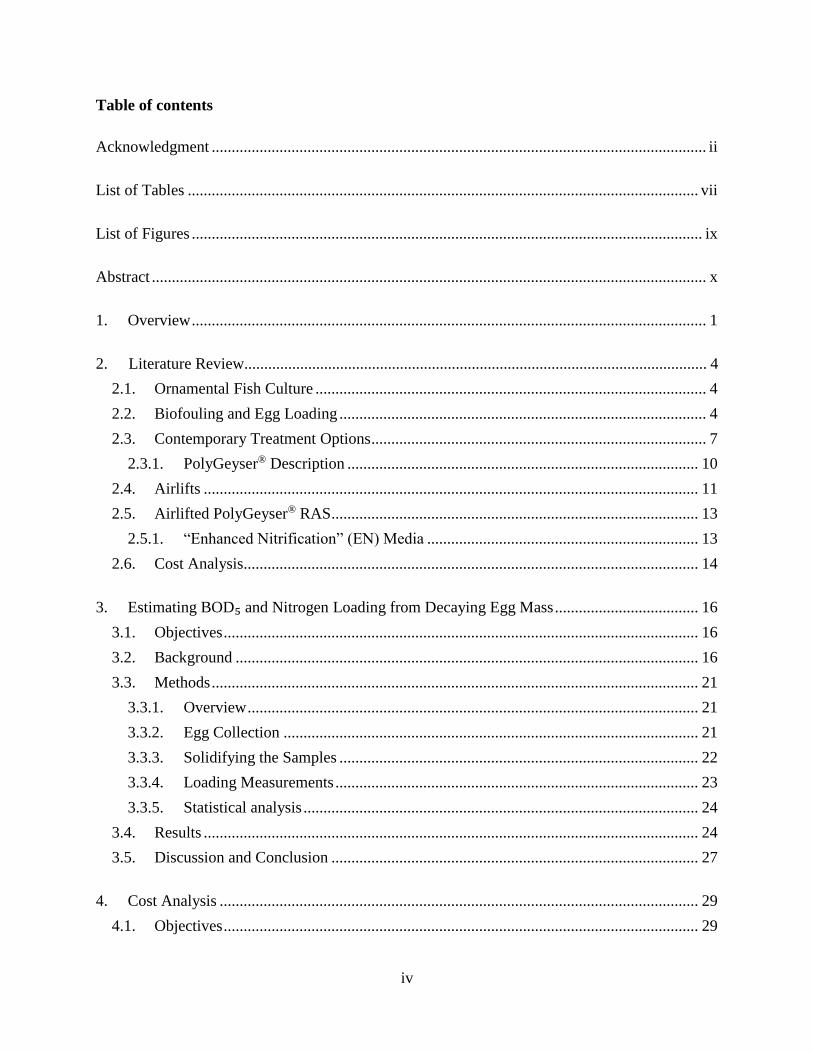
List of Tables
Table 1: Nine marine and freshwater fish species of eggs were sampled for the study. .............. 22
Table 2: Levels from BOD5, nitrogen, and protein for the eggs of all 8 species tested................ 24
Table 3: Mean BOD Tukey's Studentized Range (HSD) test for 8 species tested shows 4 different
groups (A-D). ................................................................................................................................ 25
Table 4: Nitrogen Tukey's Studentized Range (HSD) test for 8 species tested shows 4 different
groups (A-D). ................................................................................................................................ 26
Table 5: Protein Tukey's Studentized Range (HSD) test for 8 species tested shows 3 different
groups (A-C) ................................................................................................................................. 27
Table 6: Catfish and cobia displayed no significant differences from bala shark eggs for each test
....................................................................................................................................................... 28
Table 7: Measurements from Sumner (2000) were set to accommodate the RAS configuration for
growout buildings. ........................................................................................................................ 37
Table 8: Growout air flow requirements define the blower’s sizing. ........................................... 41
Table 9: Growout airlifted PolyGeyser® design criteria adapted from Malone (2013b) .............. 41
Table 10: Physical description of RAS growout........................................................................... 42
Table 11: Physical description of a fingerling tank ...................................................................... 43
Table 12: The startup of tanks is staggered to ensure a steady output of harvest fish. ................. 45
Table 13: Miscellaneous building and equipment costs other than growout capital costs ........... 46
Table 14: Capital cost for two fingerling facility.......................................................................... 48
Table 15: Annual operating cost for fingerling............................................................................. 50
Table 16: Growout capital cost per facility ................................................................................... 52
Table 17: Annual growout production cost .................................................................................. 53
Table 18: Annual operation costs for purge tanks ........................................................................ 55
Table 19: Capital costs for purge tanks......................................................................................... 56
Table 20: Unit cost per building obtained from NVP ................................................................... 57
Table 21: Life-cycle cost for the facility ....................................................................................... 58
viii
Table 22: Facility Equivalent Equipment costs over 30 year period ............................................ 59
Table 23: Fingerling sizing constants per tank ........................................................................... 108
Table 24: Equations used to determine sizing (determined values) for fingerling tanks ............ 109
Table 25: Growout tank sizing constants .................................................................................... 111
Table 26: Equations used to determine sizing (determined values) for growout tanks .............. 112
Table 27: Life-cycle cost for one tank ........................................................................................ 120

ix
List of Figures
Figure 1: McDonald Jars mechanically remove dead eggs (Source: Mather, 1884) ...................... 6
Figure 2: A dead egg removing apparatus (Source: McLeary, 1949) ............................................. 7
Figure 3: RAS floating bead filters by classification (modified from Malone and Pfeiffer, 2006) 9
Figure 4: The PolyGeyser® is a pneumatically washed unit that recycles its own backwash waters
(Source: Aquaculture Systems Technologies, 2006) .................................................................... 10
Figure 5: Freeze-dried egg samples were placed in sterile jars, then added to distilled water in the
BOD bottles. ................................................................................................................................. 23
Figure 6: The facility buildings are single gable greenhouses. Dimensions (A-G) vary based on
building type (acclimation, fingerling, growout, or purging building). ........................................ 34
Figure 7: Layout of the proposed facility ..................................................................................... 35
Figure 8: Layout of a growout building ........................................................................................ 37
Figure 9: Each tank is connected to airlifts and 2 PolyGeyser® filters. ........................................ 38
Figure 10: Schemated airlifted/PolyGeyser® combination ........................................................... 39
Figure 11: The production cost is calculated to be $1.12/lb. before processing. This figure breaks
down the cost into 7 different categories. ..................................................................................... 66
Figure 12: Distribution of costs associated with growout production .......................................... 53
Figure 13: The present worth decreases as the interest rate increases. ......................................... 60
Figure 14: The annual worth increases as interest rate increases. ................................................ 61
Figure 15: The future worth increases as the interest rate increases. ............................................ 63
Figure 16: Distribution of operation costs for the proposed facility ............................................. 73
Figure 17: Distribution of capital costs for the proposed facility ................................................. 74
x
Abstract
Airlift-equipped recirculating aquaculture systems (RAS) provide water-circulation,
aeration, and degassing efficiently and reliably. This project investigated the need for biofilters in
a fish hatchery environment to address biofouling of tank water from hatching eggs. Eggs of
various fish species were selected and Biological Oxygen Demand (BOD), total Kjeldahl nitrogen
(TKN), and protein loading and content were measured and compared. Means for all samples were:
0.67±0.05g BOD₅/g, 10.89 nitrogen±0.84% and the mean protein content 69.22±3.82%. A
statistical analysis indicates that Rachycentron canadum (cobia) and Ictalurus punctatus (channel
catfish) is the most representative of the multi-species lot when compared to Balantiocheilus
melanopterus (bala shark), the targeted species for this study. Secondly, this project sought to
quantify the costs associated with domestic tilapia growout production using Airlifted
PolyGeyser® RAS technology. A cost analysis was applied to a given facility, based on feeding
rate and annual production requirements. Results indicated a capital cost of $4,887,000 for the
entire facility including $4,671,000 for RAS equipment. The annual production cost of the growout
was determined to be $953,140 for the facility. The production cost of growout is $0.93 per pound
of fish. The calculated facility equivalent equipment cost was $0.26 and the purge facility $0.1 per
pound of fish. The total production cost of the facility per pound of tilapia produced was $1.19.
The life cycle costs of the facility over period of 30 years was $25,572,000, of which feeding
represents 43% with a cost of $11,056,000. Operation cost has the second highest cost of
$5,053,000then stocking cost, of $2,373,000. The thesis presents a tabular template of costs
applicable to airlifted PolyGeyser®-equipped facilities.
1
1. Overview
Recirculating aquaculture systems (RAS) are water-efficient in that they filter and reuse
tank water. As they minimize water use, they help save millions of gallons of water each year.
Nevertheless, these husbandry systems remain relatively costly (Masser et al., 1999). RAS must
also become cost competitive with alternate production modes (ponds, raceways, pens, and cages)
to gain popularity among commercial producers. This requires efficient design of its water
treatment processes for all stages of husbandry (hatchery, nursery, and growout) (Asian Institute
of Technology, 1994; RUFORUM, 2011).
Despite attempts to understand fish oogenesis (egg formation and development) and recent
progress on manned production (human-induced) of viable fish eggs, little documentation is
available on fish species-specific eggs and larvae (Auld and Schubel, 1978; Wallace and Selman,
1990; Lubzens et al., 2010).
Although biofouling in aquaculture, which can be defined as the process by which
accumulation of organic matter stimulate bacterial blooms, is increasingly studied, most
publications are concerned with live, grown fish (Guenther et al., 2009; Huntingford et al., 2006).
Biofouling in hatcheries results from the presence of dead eggs, egg shell debris, and other organic
waste that remains in the tank after hatching. Subsequently, the ammonia level rises making the
tank water unsuitable for the remaining fry. There is a need for a filtering system that removes the
organic matter in hatcheries. Because the organic waste load differs from species to species,
filtering system design must take into consideration the species’ loading profile.
The total Kjeldahl nitrogen (TKN) provides a physicochemical characterization of water
in terms of nitrogen. TKN level includes both organic nitrogen and ammonia. Thus, TKN level is
a reliable indicator of how inhospitable the tank is.
2
The first part of this thesis addresses the sizing of biofilters in hatcheries. It seeks to develop
a species-specific egg biofouling profile. Surrogates for an endangered species’ eggs (e.g., bala
shark) were used to determine filter loading parameters for TKN and BOD. A statistical analysis
established significant similarities in loading among species. This baseline data is needed to
determine filter size relation to egg loading.
A PolyGeyser® filter captures and removes solids and dissolved organics as it proceeds to
nitrification. Using floating beads, PolyGeyser® units self-wash or self-clean as they recycle their
own backwash waters (Malone and Beecher, 2000). Frequent washing assures efficient hydraulic
conductivity. They are energy efficient due to a relatively low headloss. The units operate most
efficiently with lifts below 12 inches (Gudipati, 2005). The operation is made relatively simple,
compared to the other recirculating systems that employ multiple treatment units (Malone and
Gudipati, 2005; Malone and Beecher, 2000).
PolyGeysers® are nitrification filters that help reduce fish loss in aquaculture. The beads
filter the water, making the system operation relatively simple. The filters are fed by airlifts that
inject air into a column to lift and transport the water vertically. By doing so, they degasify (remove
the CO₂ from the water) and allow for circulation, and add O₂ water. An Airlifted PolyGeyser®
RAS combination performs all these tasks simultaneously: it nitrifies and captures and removes
solids and dissolved organics while the airlifts circulate, add oxygen, and strip carbon dioxide. It
is cost-effective and its simplicity contrasts with the complexity of most RAS designs (Masser et
al., 1999).
The second part of this thesis aims at quantifying the cost associated with large scale tilapia
growout production using airlifted PolyGeyser® RAS technology equipped tanks. A cost analysis
applicable to PolyGeyser®-equipped tanks is presented as the study provides the financial and
3
biological rationale for launching a facility. The analysis was performed with feed rate and tank
size as the major determinants of production costs.
4
2. Literature Review
Ornamental Fish Culture
Ornamental fish are a cash crop in the U.S. and worldwide (Andrews, 1990; Chapman et
al., 1997; Steinke et al., 2009). This multi-million dollar industry features the U.S. as one of the
major importers, most species coming from Southeast Asia and the Amazon region (Bruckner,
2005; Watson and Shireman, 1996; Halachmi, 2006).
Marine and freshwater ornamental species are increasingly bred and spawn in captivity.
The culture of such species is essential to the preservation of endangered species such as the bala
shark. In effect, Halachmi (2006) and Tlusty (2002) explain that the development of RAS has
allowed for a decrease in the capture of wild ornamental fish species.
Ng and Tan (1997) note that, while too scarcely found in nature, some endangered and ornamental
species have been “successfully bred in captivity and conserved.” Tlusty (2002) reports that the
current legislation favors such a situation. Indeed, as collect on of animals from public bodies of
water faces more legal restrictions, aquarium rearing of ornamental species will increase.
Nevertheless, tank aquaculture is also regulated. Southgate (2010) remarks that several
external legislative measures and regulations have been put in place to ensure biosecurity for fish
tanks, especially regarding the quality of the tank water. However, the author notes that numerous
disease-causing agents are ubiquitous in the tank itself.
Biofouling and Egg Loading
Re-creating the fish’s habitat is a complex task. Salvesen and Vadstein (1995) observe that
intensive manned incubation differs from the natural process of fish production in regards to the
exposure of eggs and larvae to bacteria. While one of the major causes of egg mortality in fish is
5
genetic deformity (Brown et al., 2010), bacteria transmission from dead eggs to the live larvae
increases fry mortality in the hatchery tank.
Ammonia is directly excreted by fish and is produced by decaying fish waste, dead fish,
and waste feed. In hatchery tanks, waste is produced both by hatching eggs, and by the decay of
dead eggs. In the oogenetic development of fish eggs, ammonium ions accumulate during the late
embryonic stages (Finn et al., 1991).
Ip et al. (2001) details the toxic effect of ammonia on fish. Many disagree on whether
seawater species are more sensitive to ammonia toxicity than freshwater species1 (Ball, 1967;
Meade, 1985; Arthur et al., 1987; Ruyet et al., 1995; Randall and Tsui, 2002). Nevertheless,
ammonia in water has been referred to as “the major toxic nitrogen form in the environment” (Ip
et al., 2001). Indeed, this nitrogen form inhibits growth, and causes the gill development disorder
hyperplasia (Ip et al., 2001; Smart, 1976; Burrows, 1964). It also hinders energy metabolism
needed for embryos to hatch and survive upon hatching. Wright and Fyhn (2001) report that
ammonia can damage the developing embryonic tissue.
In the presence of dead, decomposed eggs and debris of hatched eggs, the quality of the
water deteriorates and may pose threats to the rest of the living organisms in the tank not only in
terms of exposure to nitrogen (ammonia), but can also induce oxygen shortage (Trout Unlimited,
2010). Fish eggs possess an oxygen reservoir within the perivitellin space (below the cell
membrane). During the perivitellin space formation, external water penetrates the cell to provide
oxygen needed for proper development (Braum, 1973). Oxygen deficiency is the cause of
numerous defects in fish. Braum (1973) observed different stages of herring morphogenesis in the
1 The disparity of results is due to the multiplicity of variables: developmental stage, whether the fish is starved or
fed, water temperature, etc.
6
lower layers of the tank, where there is poor circulation between eggs. Oxygen intake normally
increases as the eggs develop, but in the instance of oxygen shortage, eggs suffered morphological
retardation, failed to hatch, and those that hatched tended to exhibit small body length. Dead,
decaying eggs constitute a build-up of biomass in the tank, which causes a high increase in oxygen
consumption, creating a septic environment for the remaining eggs. Wickett’s 1954 experiment
measured BOD of live salmon eggs in the Nile Creek and determined oxygen demand to be
between 0.00013 and 0.0003 mg/egg/hour at a temperature of 0.1° to 8.2°C. Studies such as Steer
and Moltschaniwskyj (2007) that evaluated correlation between egg mass, embryo mortality, and
biofouling with squid suggest that biofouling is not necessarily lethal for all marine species’ eggs.
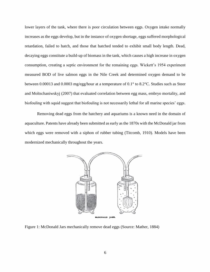
Removing dead eggs from the hatchery and aquariums is a known need in the domain of
aquaculture. Patents have already been submitted as early as the 1870s with the McDonald jar from
which eggs were removed with a siphon of rubber tubing (Titcomb, 1910). Models have been
modernized mechanically throughout the years.
Figure 1: McDonald Jars mechanically remove dead eggs (Source: Mather, 1884)
7
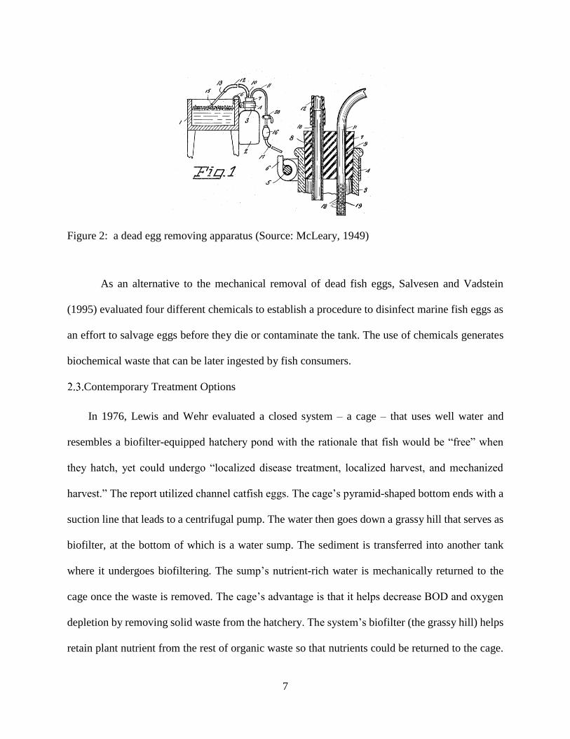
Figure 2: a dead egg removing apparatus (Source: McLeary, 1949)
As an alternative to the mechanical removal of dead fish eggs, Salvesen and Vadstein
(1995) evaluated four different chemicals to establish a procedure to disinfect marine fish eggs as
an effort to salvage eggs before they die or contaminate the tank. The use of chemicals generates
biochemical waste that can be later ingested by fish consumers.
Contemporary Treatment Options
In 1976, Lewis and Wehr evaluated a closed system – a cage – that uses well water and
resembles a biofilter-equipped hatchery pond with the rationale that fish would be “free” when
they hatch, yet could undergo “localized disease treatment, localized harvest, and mechanized
harvest.” The report utilized channel catfish eggs. The cage’s pyramid-shaped bottom ends with a
suction line that leads to a centrifugal pump. The water then goes down a grassy hill that serves as
biofilter, at the bottom of which is a water sump. The sediment is transferred into another tank
where it undergoes biofiltering. The sump’s nutrient-rich water is mechanically returned to the
cage once the waste is removed. The cage’s advantage is that it helps decrease BOD and oxygen
depletion by removing solid waste from the hatchery. The system’s biofilter (the grassy hill) helps
retain plant nutrient from the rest of organic waste so that nutrients could be returned to the cage.
8
The shortcoming of such a device is that although it removes the solid dead eggs, it does not
prevent them from fouling the water before they are removed. Inversely, chemical antifoulants
such as silicone and copper-based coatings are still being assessed and investigated (Guenther et
al., 2009; Braithwaite et al., 2007; Hodson et al., 2000), but such antifoulants do not eliminate the
need for mechanical removal of solid dead eggs.
Biological water treatment often involves the use of bacteria, such as nitrosomonas species
and nitrobacter species that oxidize the toxic ammonia into nitrites and then convert nitrites into
less toxic nitrates. Such strategy efficiently reduces water toxicity, but after extended loading, the
nitrate-rich water still needs to be changed and the tank may need cleaning (Trout Unlimited,
2010).
Fluidized beds, moving bed reactors, and floating bead filters are commonly used for
filtration of aquaculture waters (Burden, 1988; Thomasson, 1991; Sandu et al., 2002; Brindle and
Stephenson, 1996; Malone and Gudipati, 2005; Malone and Beecher, 2000; Sharrer et al., 2007;
Sharrer et al., 2010). Fluidized beds are characterized by a fixed film process that uses
hydraulically suspended sand (or plastic) as a biocarrier (Summerfelt, 2006; Weaver, 2006). These
filters remove pollutants on large surface areas, enabling oligotrophic water conditions (high
quality water required for spawning and larval rearing). However, Weaver (2006) argues that
although fluidized beds are adequate for removing soluble components, bead filters are more
efficient in removing solid waste. He uses the example of a zebra fish breeding RAS design to
show that fluidized beds provide nitrification, and that they are most effective when used in
combination with floating bead filters. Less widely used membrane biological reactors are filtering
systems that “combine activated sludge type treatment with membrane filtration” (Sharrer et al.,
2009). The membrane pores’ size determines organic retention.

9
Figure 3: RAS floating bead filters by classification (modified from Malone and Pfeiffer, 2006)
Nevertheless, the separation of liquids and solids often requires a secondary settling tank,
which is not only time-consuming, but also limits effluent quality (Hai and Yamamoto, 2011). In
municipal wastewater treatment, irreversible membrane damage has also been observed in
instances of irregular discharges (Fatone et al., 2007).
Malone and Pfeiffer (2006) present a biofilter classification of floating bead filters (Figure
3). RAS filters with moving media such as the moving bed reactor (Ødegaard et al., 1994; Rusten
et al., 2006) or the microbead filter (Timmons and Summerfelt, 1998) feature a mix of water and
air that move the filtering media in a constant manner. In RAS filters with static beads, however,
the media do not move, as the water goes through the stationary media bed. Static beds such as the
propeller-wash filter (Malone and Beecher, 2000; Chitta, 1993), the hydraulic filter (Wimberly,
1990), and the bubble-washed (Sastry et al., 1999) are further divided by their washing technique.
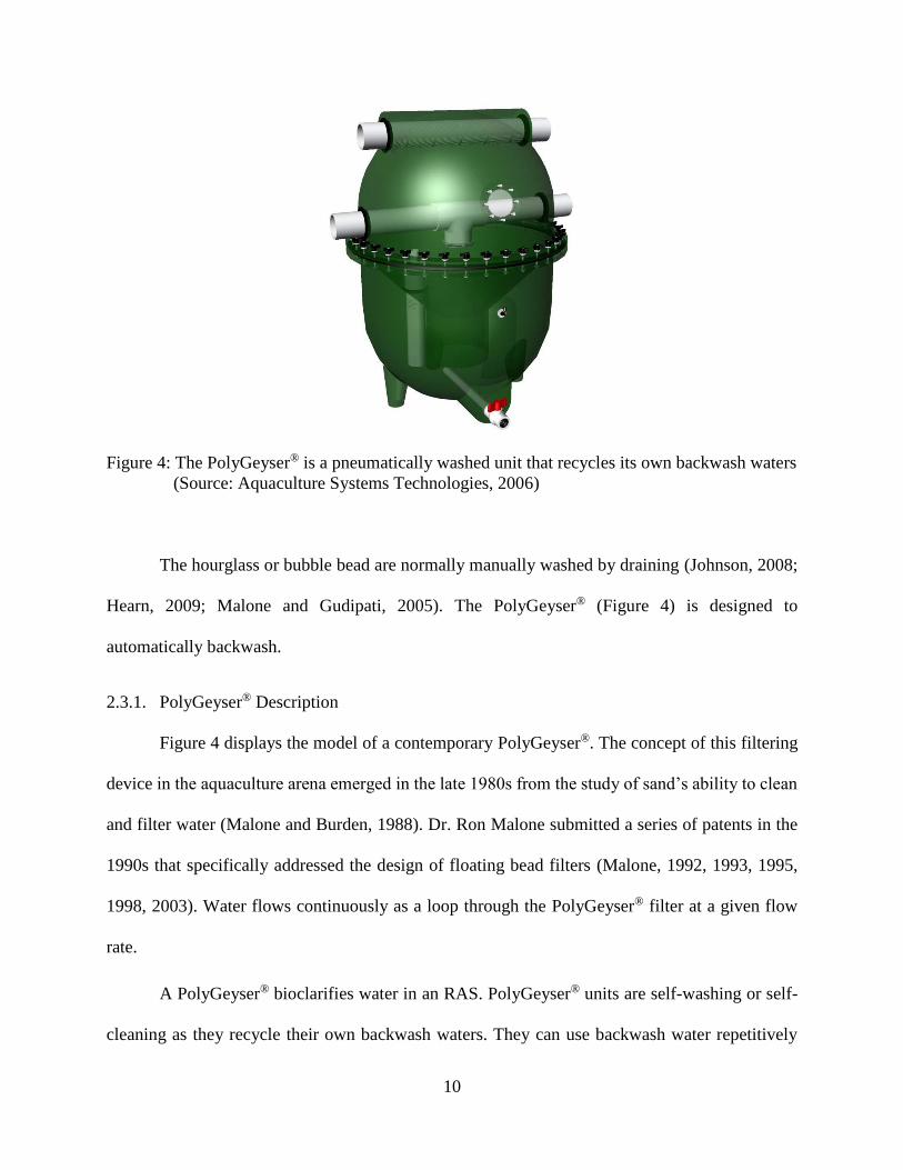
10
Figure 4: The PolyGeyser® is a pneumatically washed unit that recycles its own backwash waters
(Source: Aquaculture Systems Technologies, 2006)
The hourglass or bubble bead are normally manually washed by draining (Johnson, 2008;
Hearn, 2009; Malone and Gudipati, 2005). The PolyGeyser® (Figure 4) is designed to
automatically backwash.
2.3.1. PolyGeyser® Description
Figure 4 displays the model of a contemporary PolyGeyser®. The concept of this filtering
device in the aquaculture arena emerged in the late 1980s from the study of sand’s ability to clean
and filter water (Malone and Burden, 1988). Dr. Ron Malone submitted a series of patents in the
1990s that specifically addressed the design of floating bead filters (Malone, 1992, 1993, 1995,
1998, 2003). Water flows continuously as a loop through the PolyGeyser® filter at a given flow
rate.
A PolyGeyser® bioclarifies water in an RAS. PolyGeyser® units are self-washing or self-
cleaning as they recycle their own backwash waters. They can use backwash water repetitively
11
while retaining their nitrification capacity, which means long life and efficient hydraulic
conductivity. They can be energy efficient operating with total headlosses under 12 inches (Malone
and Gudipati, 2005).
Airlifts
The core feature of an airlift is a draft tube partially submerged in water. Air is injected
into a draft column. The air/water mixture has a low density and is pushed vertically, upwards
(lifted) by a pure water column. The pure water has a higher density and therefore exerts pressure
to eject the air/water mixture and replace the air-rich water in the tank.
The work of Gudipati (2005) evaluates the hydraulic performance of airlifts at different
flow rates and describes the characteristics of this performance. She evaluated the submergence to
lift (S: L) ratio at standard guidelines, and determined 4:1 or 80% to be the ratio at which airlifts
are most efficient.
Airlifts remove carbon dioxide (degasification), which is critical for pH control (Loyless
and Malone, 1998). Hearn (2009) established capacity/sizing standards with regards to the amount
of air needed in marine applications of airlifts. He tested performance characteristics of 20.3 cm
diameter airlifts used with warm water marine RAS. He measured that the air injection rate
corresponds to 1.3 times that of the liquid flow rate. The 20.3 cm airlift provides up to 3.1 kg
oxygen per day, while removing carbon dioxide. Hearn et al., (2009) also evaluated different airlift
sizes and produced a correspondence of oxygen and carbon dioxide transfer rates based on
different factors: pipe diameter, gas to liquid ratio, and S:L ratio. Johnson (2008) explored the
impact of different flow rates on oxygen transport for airlifted wastewater treatment applications.
In aquaculture, airlift use to sustain the rearing the marine species has flourished.
Chapman’s 1980 patent for a post larval crustacia rearing device contains an airlift that provided

12
air bubbles to the crustacia (Chapman, 1980). The device imitated the natural air supply in marine
waters. Between 1991 and 2001, Lee, Turk, and Whitson introduced a series of patents for
automated recirculating filtration systems, which airlift feature proved more cost-efficient than
those that feature electric pumps (Lee et al., 2001; Turk and Lee, 1991). The use of airlift pumps
is now widespread in the field of aquaculture, as they ensure proper water quality by circulating
and aerating water in closed systems that reuse or recirculate their water (Parker and Suttle, 1987;
Loyless and Malone, 1998; d’Orbcastel et al., 2009). Airlifts are not as energy-efficient as open
aeration systems are regarding the aeration performance, but airlifts have the advantage of
providing circulation (Loyless and Malone, 1998; Malone, 2013a). Airlifts limit the need for the
additional circulating components in an RAS.
Awari et al. (2004) determine mathematically optimal conditions of airlift pump use and
developed a computer program in which users may enter the variables of use conditions to obtain
the ideal design parameters for solid-liquid mixtures. Variables include: diameter of raising main,
immersion ratio, nozzle diameter, pressure, discharge or flow, head, and % efficiency (Timmons
and Summerfelt, 1998).
Wastewater treatment applications of pneumatic washing with the use of bead filters were
evaluated by Wagener (2003), Bellelo, (2006), and Johnson (2008). Wagener (2003) evaluated
performance of airlift-assisted secondary filtration as applied to wastewater and provides a
correspondence of biological (BOD₅) and physical (TSS) treatment based on different variables:
hydraulic filtration rate, backwash frequency, and filter configuration. The airlift/SLDM (static
low density media – bead bed) was found to produce better BOD₅ and TSS effluent qualities than
other secondary wastewater treatments, as it demonstrated higher loading capacities.

13
Airlifted PolyGeyser® RAS
Within an airlifted PolyGeyser® RAS, the PolyGeyser® nitrifies and proceeds to solids
capture and dissolved organics removal, while the airlifts circulate, add oxygen, and strip carbon
dioxide. The airlifts’ downstream position allows optimal gas transfer (Malone and Gudipati,
2005). The design approach seeks to achieve cost-effectiveness while overcoming the complex
demands imposed on RAS designs (Losordo et al., 1992), by using floating bead bioclarifiers that
simplify RAS designs (Malone and Gudipati, 2005; Malone and Beecher, 2000).
Malone and Gudipati (2005) have introduced RAS design criteria based on airlifted
PolyGeyser® technology currently employed in the United States in a number of prototype
facilities and they provide a list of airlift sizing criteria when used with a PolyGeyser®. In terms
of airlift sizing, Hearn (2009) determined 20.3 cm diameter airlifts to be adequate for multiple
stages of aquaculture: broodstock, fingerling, and growout.
In an airlifted PolyGeyser® system, airlift capacity must coordinate with the stock grown
in terms of density, volume, and feed amount. Alt (2015) studied PolyGeyser® performance as
influenced by different loading parameters such as biofilter oxygen, tank total ammonium
nitrogen, and carbon dioxide were projected and plotted against daily feed rate.
2.5.1. “Enhanced Nitrification” (EN) Media
Guerdat et al. (2010) stressed the importance of nitrification with PolyGeysers® in reducing
fish loss in fish aquaculture. The EN media was a critical element in the evolution of the airlifted
PolyGeyser® RAS treatment system. The media displayed extremely low headlosses at flow rates
used for high rate nitrification. Low bead bed headlosses, facilitate the airlift operation. Bellelo
(2006) considers Static Low Density Media (SLDM) filters used in high-density RAS, but applies
different media to the same filter configuration in a domestic wastewater treatment context. He
14
compared Enhanced Media (EN) and a KMT Kaldnes (KMT) media. As he measured post-primary
clarification BOD₅ (carbonaceous biochemical oxygen demand) and TSS (total suspended solids)
concentrations, EN was found to reduce 90% both BOD₅ and TSS. The SLDM/KMT combination
reduced 10% less. Furthermore, EN was found to generate oxygen uptake twice as high as that of
KMT, because of greater surface area per unit volume.
Cost Analysis
Large-scale tilapia farming is relatively recent in the U.S. Indeed, domestic mass
production started about 30 years ago (Josupeit, 2007; Globefish, 2015). Even though the U.S. is
still largely dependent on imports, domestic production is increasing, (USDA, 2015). The current
increase in RAS use is a turning point in the expansion of the industry (Fitzsimmons, 2000;
Molleda et al., 2007).
Watanabe et al. (2002) calculated that the greater financial yield was dependent upon feed
expenses and dissolved oxygen (DO) levels, as they noted that low DO killed or stressed fish in
ponds. Determining the total cost of fish rearing in a given facility is a complex task. To facilitate
cost estimations in RAS, Parker et al. (2012) developed a spreadsheet tool to using tilapia as an
example species. The user simply enters the numerical data that applies to his/her own facility
(yearly production, number of tanks, etc.) and the pre-recorded formulas adjust costs
automatically. Nevertheless, such tool implies that all facilities are uniform, and it allows little
room for non-listed equipment or equipment with modified voltage (which would change
electricity costs).
Held et al. (2008) analyzed the production parameters and the break-even costs for yellow
perch growout. In their study, the fish were hypothetically reared in tanks in a Texas facility.
Production parameters were expressed in terms of initial size, stocking density, feeding regime,
15
weight gain per fish, production in kg per tank, and food conversion ratio. The items considered
were related to the facility (land cost, building construction, plumbing, water system, electric
service, and labor and maintenance) and the equipment used (tanks, ponds, feeder, labor and
maintenance, etc.). Copeland et al. (2005) conducted an economic analysis on the RAS
characteristic for black sea bass production. They exposed the complexity of the various
parameters involved, such as the impact of the mortality rate on production costs and benefits of
RAS use, along with the fluctuation of market prices. Similarly, Beem and Hobbs (1995) stressed
the intricate aspect of RAS maintenance costs and their implications, as the least failure to proceed
to particularly as poor maintenance can result in rapid, dramatic production loss. The risk of
microbial contamination in RAS is also examined by Bowser et al. (1998). Shnel et al. (2002) led
a study of discharge and productivity criteria with RAS-reared tilapia. The analysis indicated that
RAS require only between 250 and 1,000 L of water per kg of fish and therefore constitutes a
source of cost and water reduction in fish production as compared to more traditional culture
methods such as ponds (Beem and Hobbs, 1995).
16
3. Estimating BOD₅ and Nitrogen Loading from Decaying Egg Mass
In hatcheries, loading and biofouling result from egg shell debris, hatching-related fluids,
and dead eggs. This organic waste decays in the tank water, leading to oxygen shortage and
nitrogen-related fouling that can affect the remaining eggs (Horvath, 1981). In this study, we
consider decomposing eggs of bala shark and characterize BOD₅ and nitrogen loading. Results
are compared with eggs of 7 other species. The results lay a foundation for design of large-scale
commercial breeding system.
Objectives
The long term objective of this effort was to develop a water treatment approach to resolve
the fouling of the water observed in bala shark breeding operations. The specific objectives of this
study were:
1. to determine the organic and nitrogen loading using eggs from abundant species
2. to determine which species produces eggs with similar waste loading characteristics to the
bala shark (Balantiocheilos melanopterus)
3. to establish the baseline waste loading expectations for a typical breeding operation laying
the foundation for a hatchery filtration system across species.
Background
Balantiocheilos melanopterus, commonly known as the bala shark (also called silver shark,
tricolor shark, or shark minnow) has an average adult length of 54 cm. Young fish are a favored
ornamental species and has been overexploited. Padmakumar et al. (2014) and Ng and Tan (1997)
describe this particular species as endangered. Early attempts to breed bala sharks in the U.S. were
complicated by high mortalities in the hatching stage (Ng and Tan, 1997). These procedures
involved the maturation of pond raised fish. The eggs were placed in tanks, hatched, and varied
17
for about one week before introduction to grow out ponds. High mortalities were attributed to poor
water quality conditions in the hatching tanks. Observations indicate that tank water used in the
bala shark breeding fouls when eggs die, jeopardizing the hatch.
While Southgate (2010) noted that numerous disease-causing agents and bacteria were
ubiquitous in the tank itself, Salvesen and Vadstein (1995) indicated that intensive manned
incubation exposed eggs and larvae to certain bacteria that they would not encounter in the natural
process. Industrial fish reproduction tends to promote fish diseases and bacteria transmission from
fish eggs to the live larvae and fish in the hatchery tank. The presence of dying and dead eggs in
the hatchery tank is a problem in that it creates a domino effect that hinders the healthy
development of all other live eggs, and fry. Brown et al. (2010) compared data on wild and captive
fish and concluded that the high rate of deformity among fish was a symptomatic response to
aquaculture-imposed conditions of hatchery-reared fish: “robust fingerling production remains a
serious impediment to the cultivation of numerous technically difficult species with otherwise
good aquaculture potential.” In addition, Brown et al. (2010) explained that the high rate of egg
mortality is mostly due to genetic deformities, and added that such a phenomenon is a typical and
growing problem of aquarium-reared ornamental fish where the gene pool was more limited.
The presence of disease-causing agents, as well as nitrifying bacteria (Madsen and
Dalsgaard, 1999; Oh et al., 2002; Malone and Pfeiffer, 2006), and salinity can also affect mortality
rates (Johnson and Katavic, 1984; Shinn et al., 2013).
Exposure to nitrogen (ammonia) and inappropriate dissolved gas concentrations (oxygen shortage,
for instance), due to the presence of dead eggs, seems to be the greatest hazard to egg survival. In
hatchery tanks more specifically, waste is produced not only by hatching eggs, but also by dead
eggs that remain in the tank. Finn et al. (1991) explained that in the oogenetic development of fish
18
eggs, ammonium ions accumulated during the late embryonic stages. The authors also suggested
that hatching eggs added more ammonia that was lethal for the remaining, unhatched eggs. In
addition, dead eggs that do not hatch and are not removed decompose and worsen the ammonia
problem (Trout Unlimited, 2010).
Ip et al. (2001) detailed the toxic effect of ammonia on fish. Ammonia inhibits growth, and
for fish, causes the gill development disorder hyperplasia (Ip et al., 2001; Smart, 1976; Burrows,
1964). It also hinders energy metabolism needed for embryos to hatch and survive upon hatching.
Wright and Fyhn (2001) more precisely reported that ammonia could damage the developing
embryonic tissue.
Ammonia nitrogen loading measurements are used as part of the physicochemical
characterization of water, and experts agree that a high level of nitrogen-derived ammonia is a
steady indicator of water toxicity (Trout Unlimited, 2010). Therefore tests such as total Kjeldahl
nitrogen (TKN) help determine water quality. For instance, high levels indicate not only protein
contamination (Vaithanomsat and Kitpreechavanich, 2008), but also potential biofouling. Nitrogen
loading is a source of great contamination for live fish (Bergheim et al., 1984; Handy and Poxton,
1993; Shinn et al., 2013). Although the direct effect of nitrogen loading on fish eggs still needs to
be further researched, it is reasonable to assume that its potentially lethal effect it has on hatched
fish is comparable or somehow proportional on fish eggs as well (Szluha, 1974). Concentrations
of nitrogen and protein in organic samples are related (Tomé and Bos, 2000). Indeed, protein
amounts and protein synthesis are controlled to a large extent by nitrogen and amino acid
concentrations (Tessari, 2006).
Although biofouling may not be directly lethal for marine species’ eggs (Steer and
Moltschaniwskyj, 2007), Hattori et al. (2004) studied the effect of varying amounts of dissolved

19
oxygen in the rearing tank. Oxygen deficiency was analyzed on a pathological viewpoint as the
cause of numerous defects in fish. In the case of fish eggs, dead, decaying eggs constitute a build-
up of biomass in the tank, which causes a high increase in oxygen consumption, and therefore
creates a septic environment for the remaining eggs (Lovegrove, 1979; Cronin et al., 1999).
Biochemical oxygen demand (BOD) corresponds to the oxygen amount aerobic organisms need
in order to break down (consume and digest) organic matter. BOD is controlled by protein levels
and, to a greater extent, the concentration of sugar and starch that enable metabolism (Church et
al., 1977; Cook et al., 2003; Wells and Wendorff, 2004). Thus, biofouled water contains more
organic matter (carbohydrates) that constitutes available energy for organisms. Wickett’s 1954
experiments measured BOD of live salmon eggs in the Nile Creek and determined oxygen demand
to be between 0.00013 and 0.0003 mg/egg/hour at a temperature of 0.1° to 8.2°C. Lowering
oxygen content or lack of water circulation was found to result in higher egg mortality.
In the case of hatchery engineering, re-creating the fish’s habitat is all the more complex
given that eggs and mature fish do not necessarily live in the same trophic level (Malone and
Pfeiffer, 2006). Malone et al. (1990) conducted a waste characterization study where they collected
water quality data regarding the aquatic environment of another endangered species, the Kemp’s
Ridley sea turtle. Water was tested for ammonia, nitrogen excretion, and BOD. The information
collected served as preliminary data in the design of a recirculating holding system for Kemp’s
Ridley sea turtles (Malone et al., 1990).
Malone and Pfeiffer (2006) illustrated the preliminary ratings needed in order to determine
biofilter sizing. They categorized filters and filter performance to match RAS applications based
on total ammonia nitrogen (TAN) loading and provide biofilter classifications based on trophic
levels from ultra-oligotrophic for larval production to hypereutrophic and acidic hypereutrophic.

20
Oligotrophic production systems are characterized by a severely limited amount of nutrients
(Malone and Pfeiffer, 2006). These systems are ideal for hatchery tanks because of the low degree
of nitrogen and organic waste which degradation leads to oxygen consumption – and/or pollutants
– at the eggs’ expense (Ip et al., 2001; Smart, 1976; Burrows, 1964; Wright and Fyhn, 2001;
Lovegrove, 1979; Cronin et al., 1999). The oligotrophic standard for biosecure fry production is
under 0.3 g N/m⁻³ (Malone and Pfeiffer, 2006; Weaver, 2006). Controlled maturation studies
indicate that some species’ eggs require an even lower (ultra-oligotrophic) TAN level <0.1 g N/m⁻³
(Watanabe et al., 1998; Malone et al., 2006).
Comparative studies suggested that fish species have comparable habitats, or habitats that
could be manipulated into similar environments for research purposes (Armstrong et al., 2003).
Smith and Noll (2009) explained that “except for temperature, salinity, and dissolved oxygen, there
are relatively few differences between species for the other water qualities.” Nevertheless, Eding
et al. (2006) expressed the need for species-specific filters, as opposed to Malone and Pfeiffer
(2006) that cited the need for unitarity in trophic level.
In RAS filters under oligotrophic conditions, biofilms are considerably thin and
heterogeneous (Malone and Pfeiffer, 2006). Diffusion to nitrifiers is relatively easy and
nitrification rates are moderate despite low TAN levels. Bacterial counts are relatively low as well
(Michaud et al., 2006). However, the oligotrophic water conditions are altered in the presence of
dead eggs, which inevitably affect the rest of the tank, especially larval fish which are extremely
sensitive to trophic water quality changes (Brown et al., 2010). As the eggs decay, there is an
increase in both carbon and nitrogen levels. The tank’s biofilms therefore thicken, and diffusion
into the biofilms subsequently slows. In terms of biofiltering capacity, increased nitrogen loading
pushes these oligotrophic RAS systems (designed for low loading) toward a mesotrophic or even
21
eutrophic condition, thereby making the filter sizing inadequate for the filtering needs of the eggs
and fry as the bacterial count rises (Malone and Pfeiffer, 2006).
More recently, Fahandezhsadi (2014) tested larval production systems with high TAN for
freshwater ornamental fish. She explored the conversion of TAN into removable microbial
biomass via heterotrophic bacteria/plastic system combination (bioplastic biofilter). These
heterotrophic filters were capable of operating as bioclarifiers in basic and acidic (pH 8 and 6.5)
ornamental fish hatchery water. No traditional dissimulatory nitrification was required.
Methods
3.3.1. Overview
Eggs of seven different species were selected for comparison to bala shark eggs. BOD,
nitrogen, and protein content were determined for each. These selected species are more abundant,
more easily and readily available, and cheaper than bala shark. Table 1 lists the species selected,
along with their aquatic habitat.
3.3.2. Egg Collection
All egg samples were outsourced in summer 2012 for the study. Eggs of potential surrogate species
(blackfin tuna, cobia, snapper, speckled trout, and yellow fin tuna) were collected from CoCo
Marine in New Orleans, Louisiana, with the help of Dr. Ed Chesney from Louisiana Universities
Marine Consortium (LUMCON). In addition, Dr. John Hargreaves from Aquaculture
Assessments, LLC. in New Orleans provided catfish and tilapia eggs. Bala shark eggs were
produced at and provided by the Institute of Food and Agriculture Sciences of the University of
Florida Cooperative Extension Service, with the assistance of Craig Watson.

22
Table 1: Nine marine and freshwater fish species of eggs were sampled for the study.
Scientific Name Common Name Water Type
Balantiocheilus melanopterus Bala Shark Freshwater
Cynoscion nebulosus Speckled trout Marine
Ictalurus punctatus Catfish Freshwater
Lutjanus campechanus Snapper Marine
Oreochromis niloticus Tilapia Freshwater
Rachycentron canadum Cobia Marine
Thunnus albacares Yellowfin tuna Marine
Thunnus atlanticus Blackfin tuna Marine
3.3.3. Solidifying the Samples
All eggs were freeze-dried in a Labconco LYPH-Lock 18 freeze-dryer and placed in a
Whirlpool® upright freezer to preserve the organic composition while removing the handling
limitations related to moisture. Freeze-dried samples were powdered via a Hamilton Beach® coffee
grinder. Powdering dry eggs increases the surface area of the particles and facilitates the
manipulation and measurement of each sample. The increased surface area facilitates the
degradation in the BOD5 test, thereby providing a worst case scenario for O2 consumption. Powder
form improved accuracy in weight measurements. Figure 5 shows the powder form of eggs from
different species.
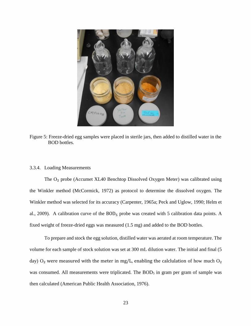
23
Figure 5: Freeze-dried egg samples were placed in sterile jars, then added to distilled water in the
BOD bottles.
3.3.4. Loading Measurements
The O₂ probe (Accumet XL40 Benchtop Dissolved Oxygen Meter) was calibrated using
the Winkler method (McCormick, 1972) as protocol to determine the dissolved oxygen. The
Winkler method was selected for its accuracy (Carpenter, 1965a; Peck and Uglow, 1990; Helm et
al., 2009). A calibration curve of the BOD5 probe was created with 5 calibration data points. A
fixed weight of freeze-dried eggs was measured (1.5 mg) and added to the BOD bottles.
To prepare and stock the egg solution, distilled water was aerated at room temperature. The
volume for each sample of stock solution was set at 300 mL dilution water. The initial and final (5
day) O₂ were measured with the meter in mg/L, enabling the calclulation of how much O₂
was consumed. All measurements were triplicated. The BOD5 in gram per gram of sample was
then calculated (American Public Health Association, 1976).
24
For TKN measurements, 1.025 g of dry weight power was measured in triplicate for each species’
egg sample into a foil paper. Samples were inserted into a nitrogen analyzer (LECO FP 528) that
analyzes organic samples and gives a reading of % nitrogen. Samples of the same weight (1.025
g) were analyzed for % protein in a LECO FP 528 as well.
3.3.5. Statistical analysis
The data acquired from the aforementioned measurements was input in SAS and an
ANOVA was conducted. A Tukey Studentized test identified similarities by grouping, based on
mean value.
Results
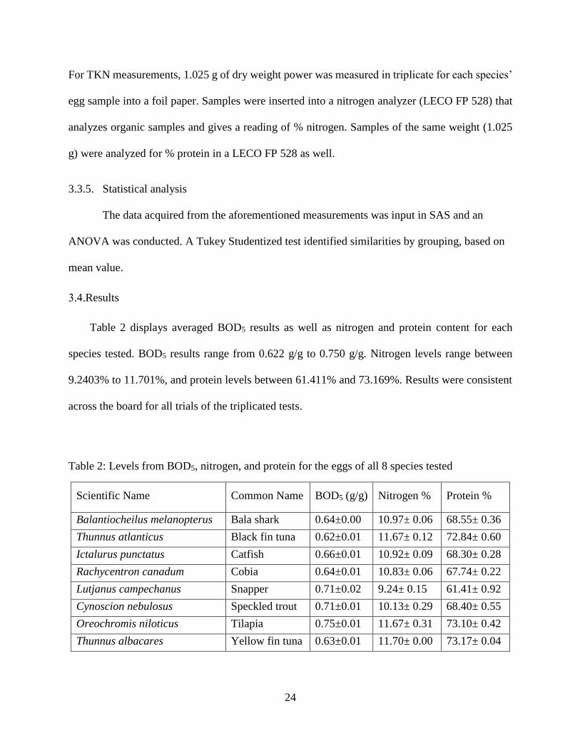
Table 2 displays averaged BOD5 results as well as nitrogen and protein content for each
species tested. BOD5 results range from 0.622 g/g to 0.750 g/g. Nitrogen levels range between
9.2403% to 11.701%, and protein levels between 61.411% and 73.169%. Results were consistent
across the board for all trials of the triplicated tests.
Table 2: Levels from BOD5, nitrogen, and protein for the eggs of all 8 species tested
Scientific Name Common Name BOD5 (g/g) Nitrogen % Protein %
Balantiocheilus melanopterus Bala shark 0.64±0.00 10.97± 0.06 68.55± 0.36
Thunnus atlanticus Black fin tuna 0.62±0.01 11.67± 0.12 72.84± 0.60
Ictalurus punctatus Catfish 0.66±0.01 10.92± 0.09 68.30± 0.28
Rachycentron canadum Cobia 0.64±0.01 10.83± 0.06 67.74± 0.22
Lutjanus campechanus Snapper 0.71±0.02 9.24± 0.15 61.41± 0.92
Cynoscion nebulosus Speckled trout 0.71±0.01 10.13± 0.29 68.40± 0.55
Oreochromis niloticus Tilapia 0.75±0.01 11.67± 0.31 73.10± 0.42
Thunnus albacares Yellow fin tuna 0.63±0.01 11.70± 0.00 73.17± 0.04
25
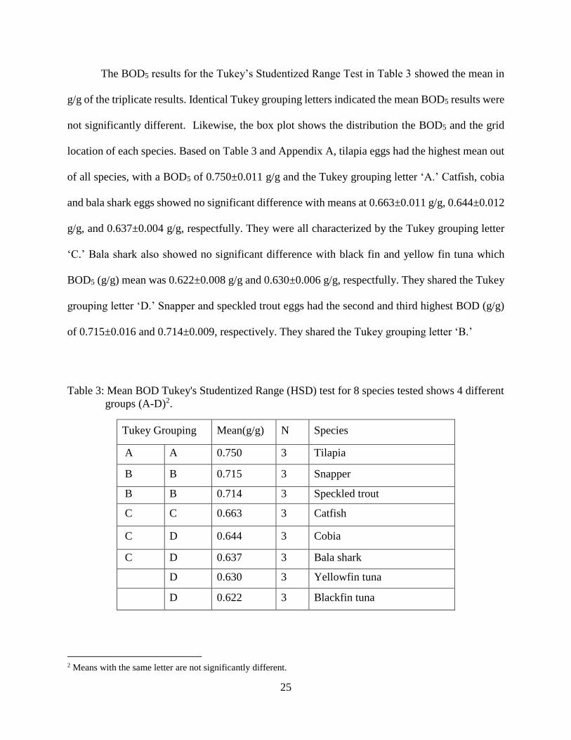
The BOD5 results for the Tukey’s Studentized Range Test in Table 3 showed the mean in
g/g of the triplicate results. Identical Tukey grouping letters indicated the mean BOD5 results were
not significantly different. Likewise, the box plot shows the distribution the BOD5 and the grid
location of each species. Based on Table 3 and Appendix A, tilapia eggs had the highest mean out
of all species, with a BOD5 of 0.750±0.011 g/g and the Tukey grouping letter ‘A.’ Catfish, cobia
and bala shark eggs showed no significant difference with means at 0.663±0.011 g/g, 0.644±0.012
g/g, and 0.637±0.004 g/g, respectfully. They were all characterized by the Tukey grouping letter
‘C.’ Bala shark also showed no significant difference with black fin and yellow fin tuna which
BOD5 (g/g) mean was 0.622±0.008 g/g and 0.630±0.006 g/g, respectfully. They shared the Tukey
grouping letter ‘D.’ Snapper and speckled trout eggs had the second and third highest BOD (g/g)
of 0.715±0.016 and 0.714±0.009, respectively. They shared the Tukey grouping letter ‘B.’
Table 3: Mean BOD Tukey's Studentized Range (HSD) test for 8 species tested shows 4 different
groups (A-D)2.
Tukey Grouping Mean(g/g) N Species
A A 0.750 3 Tilapia
B B 0.715 3 Snapper
B B 0.714 3 Speckled trout
C C 0.663 3 Catfish
C D 0.644 3 Cobia
C D 0.637 3 Bala shark
D 0.630 3 Yellowfin tuna
D 0.622 3 Blackfin tuna
2 Means with the same letter are not significantly different.
26
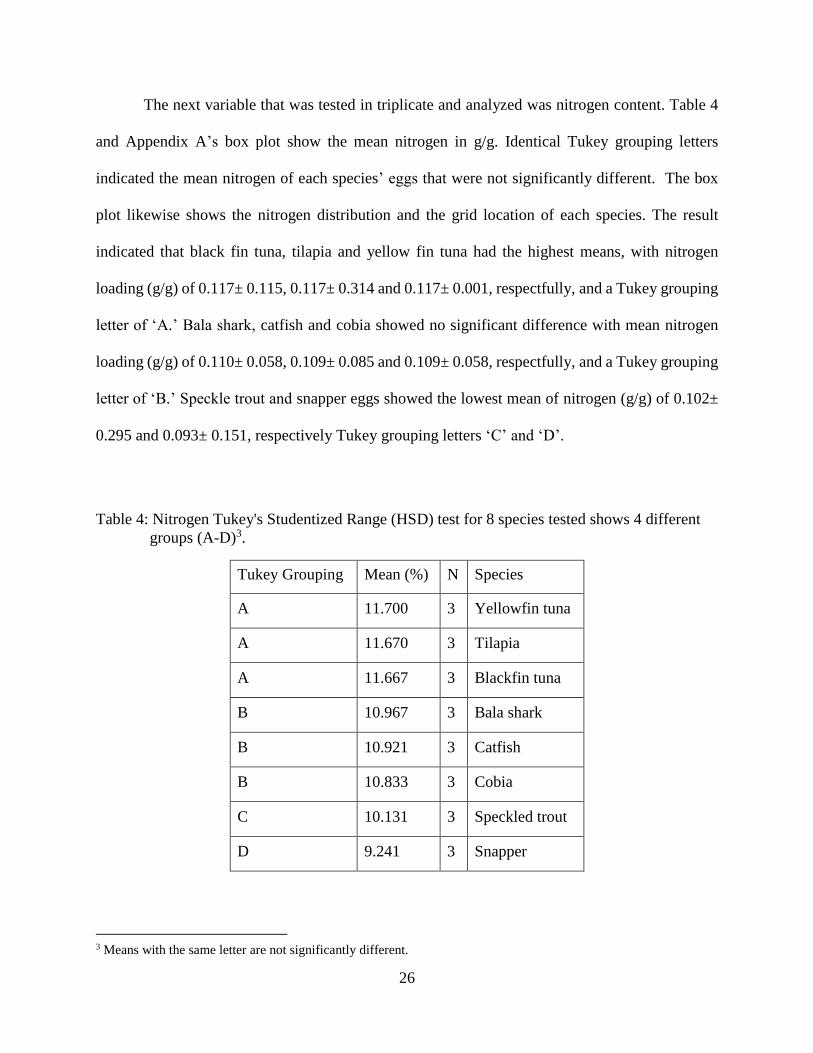
The next variable that was tested in triplicate and analyzed was nitrogen content. Table 4
and Appendix A’s box plot show the mean nitrogen in g/g. Identical Tukey grouping letters
indicated the mean nitrogen of each species’ eggs that were not significantly different. The box
plot likewise shows the nitrogen distribution and the grid location of each species. The result
indicated that black fin tuna, tilapia and yellow fin tuna had the highest means, with nitrogen
loading (g/g) of 0.117± 0.115, 0.117± 0.314 and 0.117± 0.001, respectfully, and a Tukey grouping
letter of ‘A.’ Bala shark, catfish and cobia showed no significant difference with mean nitrogen
loading (g/g) of 0.110± 0.058, 0.109± 0.085 and 0.109± 0.058, respectfully, and a Tukey grouping
letter of ‘B.’ Speckle trout and snapper eggs showed the lowest mean of nitrogen (g/g) of 0.102±
0.295 and 0.093± 0.151, respectively Tukey grouping letters ‘C’ and ‘D’.
Table 4: Nitrogen Tukey's Studentized Range (HSD) test for 8 species tested shows 4 different
groups (A-D)3.
Tukey Grouping Mean (%) N Species
A 11.700 3 Yellowfin tuna
A 11.670 3 Tilapia
A 11.667 3 Blackfin tuna
B 10.967 3 Bala shark
B 10.921 3 Catfish
B 10.833 3 Cobia
C 10.131 3 Speckled trout
D 9.241 3 Snapper
3 Means with the same letter are not significantly different.

27
Table 5: Protein Tukey's Studentized Range (HSD) test for 8 species tested shows 3 different
groups (A-C)4
Tukey Grouping Mean (%) N Species
A 73.310 3 Tilapia
A 73.170 3 Yellowfin tuna
A 72.838 3 Blackfin tuna
B 68.550 3 Bala shark
B 68.403 3 Speckled trout
B 68.320 3 Catfish
B 67.742 3 Cobia
C 61.401 3 Snapper
The final variable that was tested and analyzed is mean percent protein for all 8 species of
fish egg in triplicates. Table 5 and Appendix A’s box plot show the mean percent protein in g/g.
Again, identical Tukey grouping letters indicated the mean percent protein of each species’ eggs
that were not significantly different. The result indicated that tilapia, yellow fin and black fin tuna
eggs had the highest mean percent protein of all species with 73.10± 0.42, 73.17± 0.041 and 72.84±
0.60, respectfully, and a Tukey grouping letter of ‘A.’ Bala shark, speckle trout, catfish and cobia
eggs showed no significant difference with mean percent protein of 68.549 ± 0.362, 68.40± 0.55,
68.30± 0.28, and 67.74± 0.22, respectively, and a Tukey grouping letter of ‘B.’ Snapper eggs
showed the lowest mean percent protein of 61.41± 0.92 with a Tukey grouping letter of ‘C.’
Discussion and Conclusion
Results show a similar trend between nitrogen and protein concentrations, but a difference
between this trend and that of BOD5, as seen in Table 2. Bala shark, cobia, and catfish emerge as
the species with no statistical difference in all dependable variables test categories (BOD5,
4 Means with the same letter are not significantly different.
28
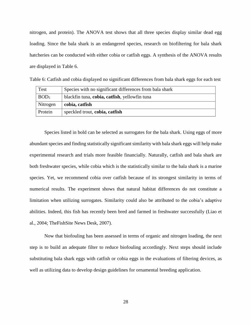
nitrogen, and protein). The ANOVA test shows that all three species display similar dead egg
loading. Since the bala shark is an endangered species, research on biofiltering for bala shark
hatcheries can be conducted with either cobia or catfish eggs. A synthesis of the ANOVA results
are displayed in Table 6.
Table 6: Catfish and cobia displayed no significant differences from bala shark eggs for each test
Test Species with no significant differences from bala shark
BOD5 blackfin tuna, cobia, catfish, yellowfin tuna
Nitrogen cobia, catfish
Protein speckled trout, cobia, catfish
Species listed in bold can be selected as surrogates for the bala shark. Using eggs of more
abundant species and finding statistically significant similarity with bala shark eggs will help make
experimental research and trials more feasible financially. Naturally, catfish and bala shark are
both freshwater species, while cobia which is the statistically similar to the bala shark is a marine
species. Yet, we recommend cobia over catfish because of its strongest similarity in terms of
numerical results. The experiment shows that natural habitat differences do not constitute a
limitation when utilizing surrogates. Similarity could also be attributed to the cobia’s adaptive
abilities. Indeed, this fish has recently been bred and farmed in freshwater successfully (Liao et
al., 2004; TheFishSite News Desk, 2007).
Now that biofouling has been assessed in terms of organic and nitrogen loading, the next
step is to build an adequate filter to reduce biofouling accordingly. Next steps should include
substituting bala shark eggs with catfish or cobia eggs in the evaluations of filtering devices, as
well as utilizing data to develop design guidelines for ornamental breeding application.
29
4. Cost Analysis
Despite growth in domestic production, over 70% tilapia consumed in the U.S. is imported
(Globefish, 2015), most of which directly from China. Commercial-scale domestic production can
be expanded with the use of RAS. Quantifying the costs and benefits of commercial aquaculture
production using RAS requires a detailed economic analysis.
RAS technologies are increasingly used for tilapia production. Indeed, a hardy species,
tilapia is adaptive to different water environments. It can withstand the presence of bacteria and
survive in adverse water conditions. It is tolerant to elevated TAN and nitrite concentrations
(Malone and Pfeiffer, 2006). In this chapter, we perform a cost analysis of growout tilapia
production on a hypothetical facility that uses airlifted PolyGeyser® RAS technology. We
determine capital costs that constitute the original investment, as well as operation costs that reflect
the financial impact of production-related variables.
Objectives
This chapter provides a framework for economic assessment in airlifted PolyGeyser® RAS,
focusing on the growout stage application of RAS. The objectives include: a) The assessment of
the direct normalized cost for Nile tilapia growout production (in dollars per lb.) for a commercial
scale airlifted PolyGeyser® RAS facility located in the southern part of the United States; b) The
mathematical determination of the influence of loan interest rate on the facility’s financial (present,
annual, and future) worth.
Background
Aquaculture is already known to be more beneficial than cattle and poultry production in
terms of nutritional and production time benefits (Helfrich and Garling, 2009). Tilapia is an
alternative to meat and other, more expensive fish species because of its suitability for intensive a

30
culture. It is tolerant to various environmental conditions (including poor water quality and saline
water) (El-Sayed, 2006). The development of U.S. intensive tilapia farming is a contemporary
phenomenon (Josupeit, 2007; FAO, 2011). North American production is on the rise, but most
tilapia consumed in the U.S. is still produced abroad, mostly in Asia and Central America (USDA,
2015). Fitzsimmons (2000) and Watanabe et al. (2002) noted that the U.S. fish production industry
was a leader in the development and engineering of recirculating techniques. RAS thus constitute
a new investment in modern-day U.S. aquaculture, as their use has become more widespread
throughout the past 30 years (Molleda et al., 2007), and are a key contributor in the expansion of
the industry.
Otoshi et al. (2003) compared shrimp growth in RAS and in ponds. Growth to growout
size was slightly lower in RAS, which could be attributable to the lack of natural productivity.
Otherwise, there were no noted drawbacks (survival, reproductive performance, or productivity
rates). The water quality was better in RAS, and RAS also offered a more controlled environment
in terms of temperature and ventilation. Nevertheless, due to more rapid growth, ponds provided
faster pay back. The study also showed that RAS offer biosecurity, whereas the presence of any
infection agent could jeopardize the survival of an entire harvest in other production systems.
While Otoshi et al. (2003) provided experimental results; Moss and Leung (2006) studied the
economics of pond v. RAS shrimp production. They explained that RAS shrimp production was
significantly cheaper ($4.38/kg v. $6.71/kg), reflecting multiple harvests and biosecurity.
Helfrich and Libey (1991) who had predicted that tilapia could be the cash crop of the 21st
century also compared production management and costs in different systems. RAS provided a
more controlled environment as opposed to ponds where the fish was more exposed and vulnerable
to environmental changes. This controlled environment allows for year-long production and
31
multiple harvests, and therefore increases profit (Helfrich and Libey, 1991). Furthermore, with less
water usage, RAS are more appropriate for intensive production. Overall better flavor is noted with
RAS-produced tilapia, because ponds contain contaminants detectable in fish taste. In addition,
RAS require less space, which reduces land costs. However, RAS have a higher initial capital cost.
They require more skilled labor, which increases operation costs. Moreover, RAS are more
dependent on mechanical and electric power, thus a power outage can compromise the entire
production.
Malone and Gudipati (2005) introduced RAS design criteria based upon an airlifted
PolyGeyser® technology that is currently being employed in the United States in a number of
prototype facilities. The design approach seeks to achieve cost-effectiveness while overcoming the
complex demands imposed on RAS designs (Masser et al., 1999). Malone (2013b) discussed
design modifications needed when applying empirical laboratory data to actual commercial scale
tilapia production facilities. Commercial practice demonstrated that an increase in airlift sizing
criterion (from 1 ft/sec to 1.5 ft/sec) for airlifts with diameters ≥ 6 in. was possible. Cost
considerations (the high price of reducer fittings) led to a reduction of the approach pipes’ design
velocities (from 2-3 ft/sec to 1.5 ft/sec criterion). The PolyGeyser® sizing criterion was unchanged
(1.5 lbs feed/ft³/day), but it is observed that the large scale PolyGeysers® not reach their maximum
capacity in early facilities. This was due to limitations imposed by, among other secondary factors,
water volume (>200 gal. /lb. feed/day) or blower capacity (> 4 cfm/lb. feed/day). The study
recommended “continued refinement in design criterion.”
Malison and Held (2006) and Held et al. (2008) analyzed the production parameters and
the break-even costs for yellow perch growout in farm ponds and in RAS, respectively. Production
parameters were expressed in terms of initial size, stocking density, feeding regime, weight gain
32
per fish, production in kg per tank, and food conversion ratio. They included an analysis of
investment costs. The items considered were related to the facility (land cost, building
construction, plumbing, water system, electric service, and labor and maintenance) and the
equipment used (tanks, ponds, feeder, labor and maintenance, etc.). The authors also included an
editable spreadsheet. For RAS production, profitability started at $3.30/lb., but the break-even cost
decreased with time, based on the number of cycles input in the spreadsheet.
Copeland et al., (2005) conducted an economic analysis on the RAS characteristic for black
sea bass production. They examined the complexity of the various parameters involved, including
the impact of the mortality rate on production costs and benefits of RAS use, along with the
fluctuation of market prices. Similarly, Beem and Hobbs (1995) stress the intricate aspect of RAS
maintenance costs and their implications, as even a small failure to follow maintenance procedures
can result in rapid, dramatic production loss. The risk of microbial contamination in RAS was
examined by Bowserg et al. (1998).
Helfrich and Libey (1991) conducted a comparative analysis of RAS, ponds, and raceways.
RAS were viewed favorably for their ability to rear fish at higher densities, for their controllable
environment, and high water reuse. New water is used only to compensate for evaporation and
sludge removal. The study of Molleda et al. (2007) compared water quality and consumption in
RAS with that in Limited Reuse Systems (LRS) for a culture of Arctic charr. Results indicate a
better water quality with LRS but greater water consumption, which resulted in higher costs.
Losordo and Westerman (1994) used STELLA modelling language to complete a computerized
simulation of small-scale RAS tilapia production featuring a floating bead filter with a rotating
biological contactor used in series. Dissolved oxygen was added externally. The simulated facility
included both fingerling and growout systems. Their simulation indicates a production cost of

33
$1.27/lb. Based on their model sensitivity analysis, “improvements in the performance efficiency
of system components [do] not greatly affect fish production cost.” However, variables that can
significantly reduce cost are feed cost reduction, feed conversion ratio improvement. Greater gains
are also dependent upon production capacity and decreased investment costs.
The relative cost of recirculation pertaining to the alternative systems (ponds and net pens)
can be expected to decrease, even though baseline costs will continue to increase (Malone and
Gudipati, 2005). Malone (2013a) noted that raceway tanks can be costly, and he contrasted axial
flow pumps that have a low operation cost but a high initial capital cost, with airlift pumps that are
inexpensive and considerably energy efficient. In light of such decrease in cost, Malone and
Gudipati (2005) predict an increased use of recirculating systems use as well as a diversification
of their uses into growout use. Although bead media have been criticized for being relatively
expensive to produce (Gutierrez-Wing et al., 2007; Castilho et al., 2009), investment costs for bead
filter-equipped RAS are also expected to decrease (Chanprateep 2010, Fahandezhsadi, 2014).
Parker et al. (2012) developed a spreadsheet tool to facilitate cost estimations in RAS using tilapia
as an example species. Helfrich and Garling (1985) noted that when determining the cost of
aquaculture production, the planning stage is quite complex because numerous biological,
economic, and legal factors must be taken into consideration. They explained that preliminary
research on feasibility constitutes the first step to take to ensure the success of any commercial
aquaculture project. To determine the total production cost, one must also consider additional
parameters related to capital investment costs, such as: equipment cost (tanks, pipes, etc.), material
cost or items that help sustain the process (e.g., fish, eggs, feeding, etc.), installation cost, working
capital, project engineering, and management (rate charged by fishery engineers, researchers,
lawyers, and other consultants).
34
Proposed Facility
The proposed facility is a set of buildings assumed to be already equipped with a water
source (water well). The farm campus is made up of polyethylene greenhouses5. The greenhouse
design presented in Figure 6 is similar for all 6 buildings. It is adapted from the Sumner (2000)6,
and greenhouse heating requirements are obtained from a template developed by Jones (2010).
Figure 7 is a blueprint of the spatial arrangement of the facility.
Figure 6: The facility buildings are single gable greenhouses. Dimensions (A-G) vary based on
building type (acclimation, fingerling, growout, or purging building).
5 Another feasible option would be the conversion of an existing fowl farm. The greenhouse design approach was
elected because of its ability to reduce light and heating costs. 6 Sumner (2000) explained that heating requirements can be drastically reduced when the buildings are joined as
gutter connected gable greenhouses, for single buildings because of the increased risk of spreading contamination
that incurs when buildings share a common wall.

35
Figure 7: Layout of the proposed facility
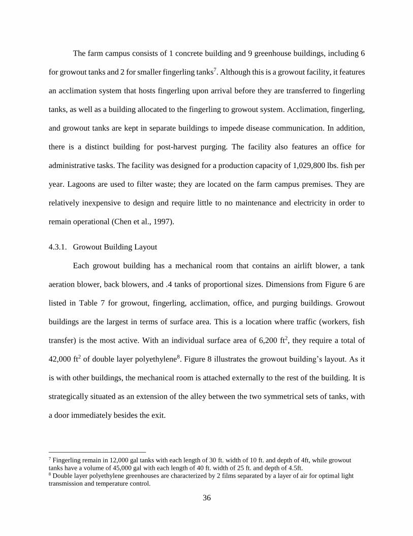
36
The farm campus consists of 1 concrete building and 9 greenhouse buildings, including 6
for growout tanks and 2 for smaller fingerling tanks7. Although this is a growout facility, it features
an acclimation system that hosts fingerling upon arrival before they are transferred to fingerling
tanks, as well as a building allocated to the fingerling to growout system. Acclimation, fingerling,
and growout tanks are kept in separate buildings to impede disease communication. In addition,
there is a distinct building for post-harvest purging. The facility also features an office for
administrative tasks. The facility was designed for a production capacity of 1,029,800 lbs. fish per
year. Lagoons are used to filter waste; they are located on the farm campus premises. They are
relatively inexpensive to design and require little to no maintenance and electricity in order to
remain operational (Chen et al., 1997).
4.3.1. Growout Building Layout
Each growout building has a mechanical room that contains an airlift blower, a tank
aeration blower, back blowers, and .4 tanks of proportional sizes. Dimensions from Figure 6 are
listed in Table 7 for growout, fingerling, acclimation, office, and purging buildings. Growout
buildings are the largest in terms of surface area. This is a location where traffic (workers, fish
transfer) is the most active. With an individual surface area of 6,200 ft2, they require a total of
42,000 ft2 of double layer polyethylene8. Figure 8 illustrates the growout building’s layout. As it
is with other buildings, the mechanical room is attached externally to the rest of the building. It is
strategically situated as an extension of the alley between the two symmetrical sets of tanks, with
a door immediately besides the exit.
7 Fingerling remain in 12,000 gal tanks with each length of 30 ft. width of 10 ft. and depth of 4ft, while growout
tanks have a volume of 45,000 gal with each length of 40 ft. width of 25 ft. and depth of 4.5ft. 8 Double layer polyethylene greenhouses are characterized by 2 films separated by a layer of air for optimal light
transmission and temperature control.
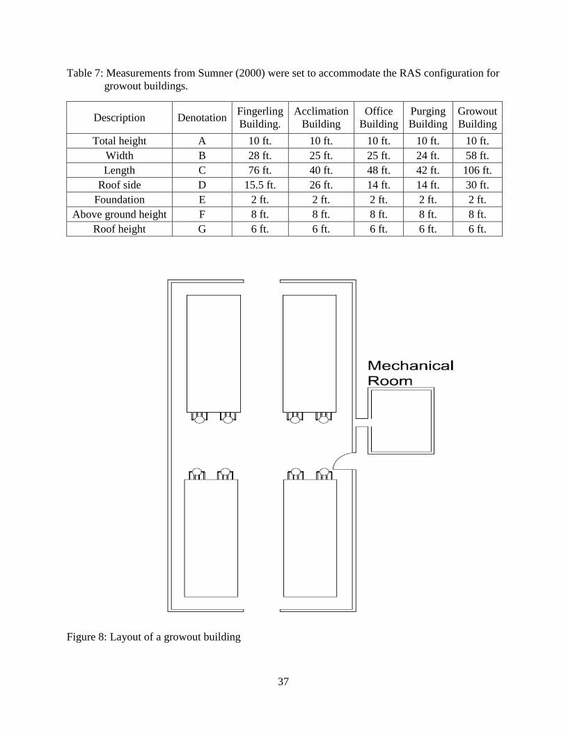
37
Table 7: Measurements from Sumner (2000) were set to accommodate the RAS configuration for
growout buildings.
Description Denotation Fingerling
Building.
Acclimation
Building
Office
Building
Purging
Building
Growout
Building
Total height A 10 ft. 10 ft. 10 ft. 10 ft. 10 ft.
Width B 28 ft. 25 ft. 25 ft. 24 ft. 58 ft.
Length C 76 ft. 40 ft. 48 ft. 42 ft. 106 ft.
Roof side D 15.5 ft. 26 ft. 14 ft. 14 ft. 30 ft.
Foundation E 2 ft. 2 ft. 2 ft. 2 ft. 2 ft.
Above ground height F 8 ft. 8 ft. 8 ft. 8 ft. 8 ft.
Roof height G 6 ft. 6 ft. 6 ft. 6 ft. 6 ft.
Figure 8: Layout of a growout building
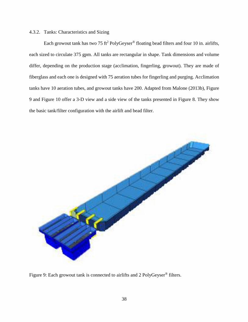
38
4.3.2. Tanks: Characteristics and Sizing
Each growout tank has two 75 ft2 PolyGeyser® floating bead filters and four 10 in. airlifts,
each sized to circulate 375 gpm. All tanks are rectangular in shape. Tank dimensions and volume
differ, depending on the production stage (acclimation, fingerling, growout). They are made of
fiberglass and each one is designed with 75 aeration tubes for fingerling and purging. Acclimation
tanks have 10 aeration tubes, and growout tanks have 200. Adapted from Malone (2013b), Figure
9 and Figure 10 offer a 3-D view and a side view of the tanks presented in Figure 8. They show
the basic tank/filter configuration with the airlift and bead filter.
Figure 9: Each growout tank is connected to airlifts and 2 PolyGeyser® filters.

39
Figure 10: Schemated airlifted/PolyGeyser® combination
Adapted from Malone (2013b)
Configuration and Components
The proposing 75 ft³ PolyGeyser® bead filter models, built by Arrowhead Fiberglass
Industry, LLC, located in Canton City, Colorado. The filters are filled with “Enhanced
Nitrification” media configured for airlift operation produced by Aquaculture Systems
Technologies in New Orleans, Louisiana. Bioclarification and recirculation in Figure 10 occurs in
two modes. First, during normal operation, water travels from the tank to the PolyGeyser® through
the beads to the airlift’s draft tube and back into the tank. This allows the bacteria on the beads to
feed off of the contaminants in the water and thus clean it. The second mode of operation is
backwashing. During normal operation, air is constantly input to the charge chamber. When
enough air has accumulated in the charge chamber, the air releases, forcing bubbles through the
bead bed. The beads mix up and the backwash water flows into the charge chamber. As normal
filtration resumes, solids settle out of the backwash water, forming a sludge in the sludge storage
basin. Above this basin, each PolyGeyser® has a bottom drain located at its center. The drain is
“connected to a drain line, which [discharges] solids and sludge” to a storing basin (Timmons and
Sludge storage basin
Intermittent air injector for sludge removal
Draft tube
40
Ebeling, 2006). The backwash waters are displaced by the entering air chamber. In this manner,
backwash waters are recycled to the tank.
The speed of sludge flushing also depends on the hydraulic retention time (HRT), that is,
the throughput flow rate or turnover time. The higher the rate, the more oxygen is provided, and
the faster the sludge can be flushed away. With tanks the size of those in the proposed facility, the
HRT is relatively low, compared to smaller tanks. Therefore, the airlift’s inlet and outlet injection
compensates for the otherwise low HRT and helps ensure proper water conditions and sludge
removal (Timmons and Ebeling, 2006).
Growout Tank Design
Design constants are determined from step-by-step engineering analysis (Malone, 2013b)9.
Each growout tank is furnished with two PolyGeyser® filters. One cubic foot of beads can process
the wastes of 2.25 lbs. of feed per day under expert management. In practice, the filters operate at
67% efficiency, thus one cubic foot of beads will support 67% of 2.25 lbs. of feed, that is, 1. 5 lb.
/ft3 However, with 45,000 gallon tanks, the peak carrying capacity for feed is 225 lbs. The feed
load determines the size of all components, as constants are multiplied by feed loading. Appendix
C: Fingerling and Growout Assumptions shows that the recirculation rate (amount of water filtered
by the PolyGeyser®) is a direct multiplication of the daily amount of feed and the constant
circulation rate (amount of water per minute that moves through the airlift). In the design, we used
an airflow of 3 cfm with a safety factor of 1.5. The amount of oxygen consumed is derived from
the amount of feed administered. Knowing the oxygen consumed allows calculation of the RAS
air flow rate.
9 Studies such as Gudipati (2005), Hearn (2009), and Johnson (2008) provide a reliable empirical analysis
framework that provides safe assumptions.

41
Table 8 shows the correlation between air flow and blower power (which can be translated
into electricity costs). As shown in Table 9 that details the design criteria for growout tanks, we
used recirculation rate of 7.5 gpm. feed/day and an airflow of 3 cfm lp feed per day and water flow
rate are correlated (Malone, 2013b), calculations of the needed flow rate and the airlift cross-
section area (in ft²) will be matched with corresponding pipe diameter and length. Table 10
provides numerical values for the growout tanks’ different characteristics.
Table 8: Growout air flow requirements define the blower’s sizing.
Requirement cfm air flow hp blower power
In-tank aeration per tank 465 7
Airlifts per tank 465 7
In-tank aeration for the facility 22,300 200
Airlifts for the facility 22,300 200
Table 9: Growout airlifted PolyGeyser® design criteria adapted from Malone (2013b)
Component Criterion
English Units. Metric
Tank (recirculation
rate)
200 gal./lb. feed/day 1.67 m3/kg feed/day
PolyGeyser® 0.67 ft3-beads/lb. feed/day 0.042 m3 bead/kg feed/day
Recirculation flow 7.5 gpm/lb. feed/day 38 Lpm/kg feed day
Airlift area 1.5 ft/sec or 450 gpm/ft2 0.46 m/sec
Lift (L) 12-15” 30-38 cm
Submergence (S) 4*L 4*L
Blower Volume 3 cfm/1b feed/day 187 Lpm/kg feed/day
Blower Pressure 5*L 5*L
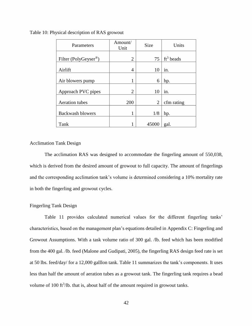
42
Table 10: Physical description of RAS growout
Parameters Amount/
Unit Size Units
Filter (PolyGeyser®) 2 75 ft3 beads
Airlift 4 10 in.
Air blowers pump 1 6 hp.
Approach PVC pipes 2 10 in.
Aeration tubes 200 2 cfm rating
Backwash blowers 1 1/8 hp.
Tank 1 45000 gal.
Acclimation Tank Design
The acclimation RAS was designed to accommodate the fingerling amount of 550,038,
which is derived from the desired amount of growout to full capacity. The amount of fingerlings
and the corresponding acclimation tank’s volume is determined considering a 10% mortality rate
in both the fingerling and growout cycles.
Fingerling Tank Design
Table 11 provides calculated numerical values for the different fingerling tanks’
characteristics, based on the management plan’s equations detailed in Appendix C: Fingerling and
Growout Assumptions. With a task volume ratio of 300 gal. /lb. feed which has been modified
from the 400 gal. /lb. feed (Malone and Gudipati, 2005), the fingerling RAS design feed rate is set
at 50 lbs. feed/day/ for a 12,000 galllon tank. Table 11 summarizes the tank’s components. It uses
less than half the amount of aeration tubes as a growout tank. The fingerling tank requires a bead
volume of 100 ft3/lb. that is, about half of the amount required in growout tanks.
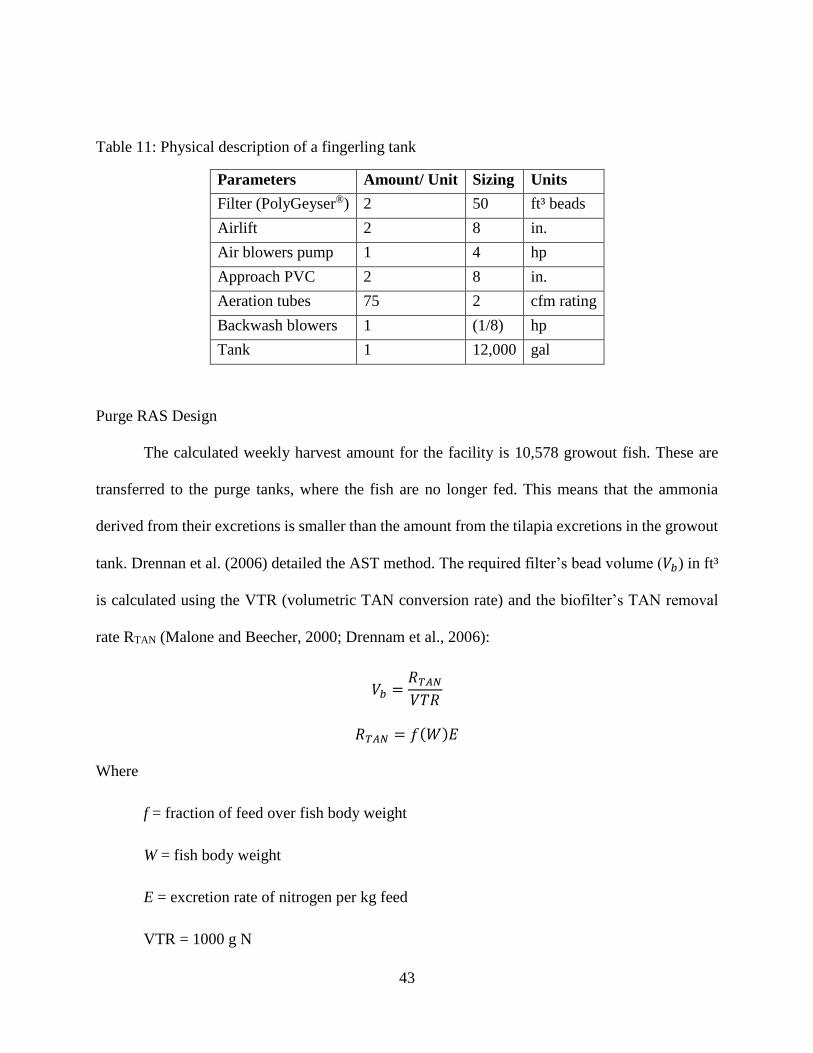
43
Table 11: Physical description of a fingerling tank
Parameters Amount/ Unit Sizing Units
Filter (PolyGeyser®) 2 50 ft³ beads
Airlift 2 8 in.
Air blowers pump 1 4 hp
Approach PVC 2 8 in.
Aeration tubes 75 2 cfm rating
Backwash blowers 1 (1/8) hp
Tank 1 12,000 gal
Purge RAS Design
The calculated weekly harvest amount for the facility is 10,578 growout fish. These are
transferred to the purge tanks, where the fish are no longer fed. This means that the ammonia
derived from their excretions is smaller than the amount from the tilapia excretions in the growout
tank. Drennan et al. (2006) detailed the AST method. The required filter’s bead volume (𝑉𝑏) in ft³
is calculated using the VTR (volumetric TAN conversion rate) and the biofilter’s TAN removal
rate RTAN (Malone and Beecher, 2000; Drennam et al., 2006):
𝑉𝑏 =𝑅𝑇𝐴𝑁
𝑉𝑇𝑅
𝑅𝑇𝐴𝑁 = 𝑓(𝑊)𝐸
Where
f = fraction of feed over fish body weight
W = fish body weight
E = excretion rate of nitrogen per kg feed
VTR = 1000 g N
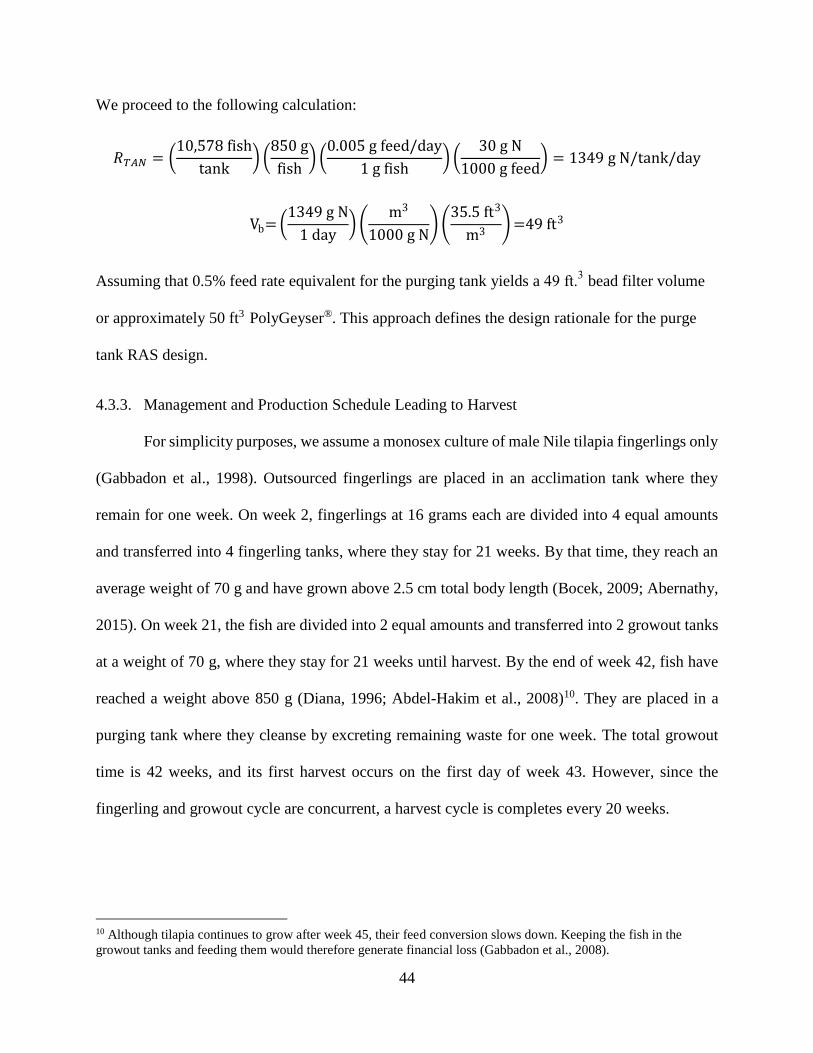
44
We proceed to the following calculation:
𝑅𝑇𝐴𝑁 = (10,578 fish
tank) (
850 g
fish) (
0.005 g feed/day
1 g fish) (
30 g N
1000 g feed) = 1349 g N/tank/day
Vb= (1349 g N
1 day) (
m3
1000 g N) (
35.5 ft3
m3) =49 ft3
Assuming that 0.5% feed rate equivalent for the purging tank yields a 49 ft.3 bead filter volume
or approximately 50 ft3 PolyGeyser®. This approach defines the design rationale for the purge
tank RAS design.
4.3.3. Management and Production Schedule Leading to Harvest
For simplicity purposes, we assume a monosex culture of male Nile tilapia fingerlings only
(Gabbadon et al., 1998). Outsourced fingerlings are placed in an acclimation tank where they
remain for one week. On week 2, fingerlings at 16 grams each are divided into 4 equal amounts
and transferred into 4 fingerling tanks, where they stay for 21 weeks. By that time, they reach an
average weight of 70 g and have grown above 2.5 cm total body length (Bocek, 2009; Abernathy,
2015). On week 21, the fish are divided into 2 equal amounts and transferred into 2 growout tanks
at a weight of 70 g, where they stay for 21 weeks until harvest. By the end of week 42, fish have
reached a weight above 850 g (Diana, 1996; Abdel-Hakim et al., 2008)10. They are placed in a
purging tank where they cleanse by excreting remaining waste for one week. The total growout
time is 42 weeks, and its first harvest occurs on the first day of week 43. However, since the
fingerling and growout cycle are concurrent, a harvest cycle is completes every 20 weeks.
10 Although tilapia continues to grow after week 45, their feed conversion slows down. Keeping the fish in the
growout tanks and feeding them would therefore generate financial loss (Gabbadon et al., 2008).
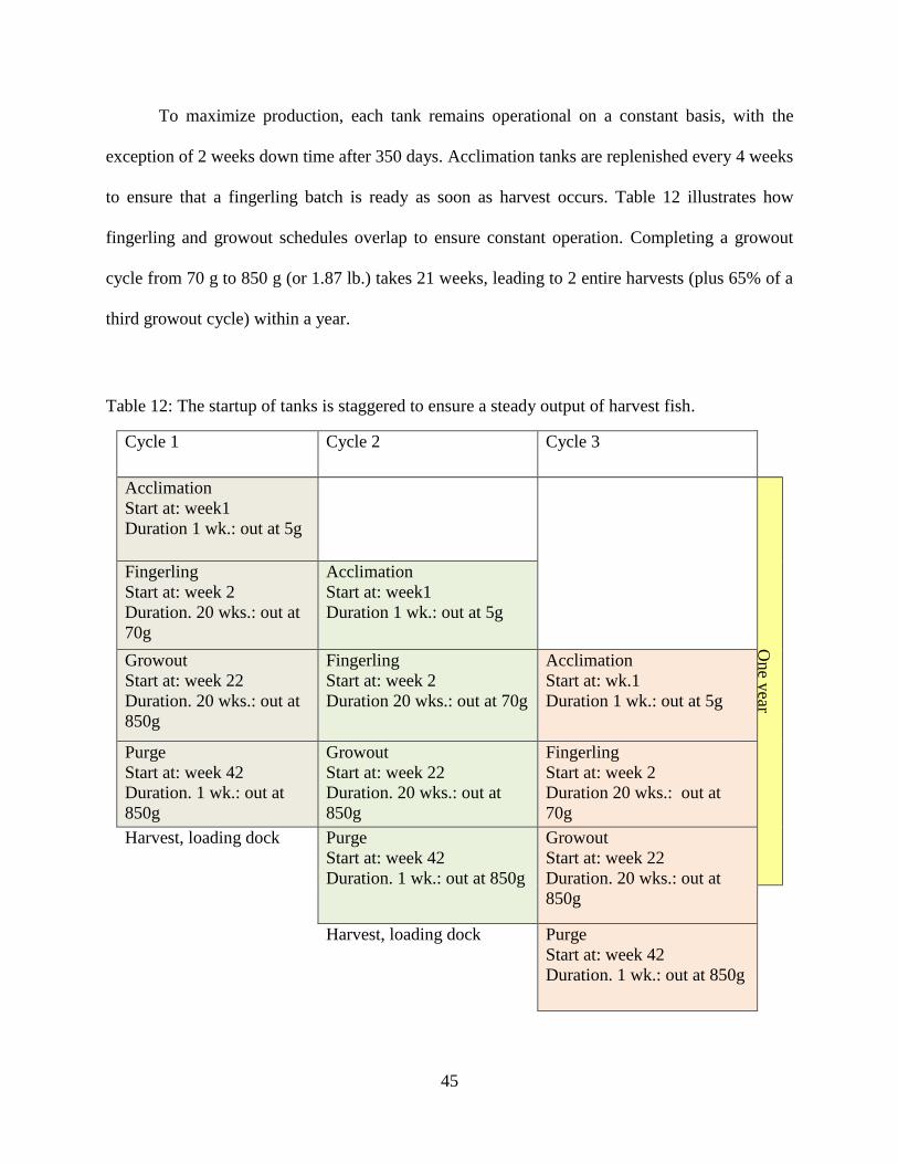
45
To maximize production, each tank remains operational on a constant basis, with the
exception of 2 weeks down time after 350 days. Acclimation tanks are replenished every 4 weeks
to ensure that a fingerling batch is ready as soon as harvest occurs. Table 12 illustrates how
fingerling and growout schedules overlap to ensure constant operation. Completing a growout
cycle from 70 g to 850 g (or 1.87 lb.) takes 21 weeks, leading to 2 entire harvests (plus 65% of a
third growout cycle) within a year.
Table 12: The startup of tanks is staggered to ensure a steady output of harvest fish.
Cycle 1 Cycle 2 Cycle 3
Acclimation
Start at: week1
Duration 1 wk.: out at 5g
One y
ear
Fingerling
Start at: week 2
Duration. 20 wks.: out at
70g
Acclimation
Start at: week1
Duration 1 wk.: out at 5g
Growout
Start at: week 22
Duration. 20 wks.: out at
850g
Fingerling
Start at: week 2
Duration 20 wks.: out at 70g
Acclimation
Start at: wk.1
Duration 1 wk.: out at 5g
Purge
Start at: week 42
Duration. 1 wk.: out at
850g
Growout
Start at: week 22
Duration. 20 wks.: out at
850g
Fingerling
Start at: week 2
Duration 20 wks.: out at
70g
Harvest, loading dock Purge
Start at: week 42
Duration. 1 wk.: out at 850g
Growout
Start at: week 22
Duration. 20 wks.: out at
850g
Harvest, loading dock Purge
Start at: week 42
Duration. 1 wk.: out at 850g

46
The design criteria and management plans for fingerling and growout systems are based
on a goal of harvesting 1,029,800 lbs. fish per year, that is, 550,038 fish weighing an average of
1.87 lb. each. This implies the number of fingerling required each year is 610,542. The amount of
fish harvested is commensurate with proper management and up keep base on disease prevention
and waste water management.
Cost Analysis: Results
4.4.1. Overview
Capital or investment cost refers to the monetary amount invested into the purchase of
items needed to realize a project (such as land, machinery, equipment, transportation, facility,
equipment, etc.). In other words, we consider items that must be initially purchased or rented.
These amounts are fixed and generally constitute one-time expenses (Boehlje and Ehmke, 2005).
Table 13: Miscellaneous building and equipment costs other than growout capital costs
Item Cost Comment
Fingerling Building $44,000.00 Two Greenhouse double liner 4400 ft² × $10
Acclimation Building $20,000.00 Greenhouse double liner 2000 ft² × $10
Purge Building $10,000.00 Greenhouse double liner 1000 ft² × $10
Office / Storage Building $43,024.04 for a 1200 ft² warehouse office
Fingerling RAS 441,700.00
Design capacity to accommodate the growout
amount
Acclimation RAS $52,020.00
Design capacity to accommodate the fingerling
amount
Purge RAS $22,920.00 Design criteria based estimated TAN excretion
Labor $33,000.00
Labor cost for construction installation and piping
fitting
47
Table 13 shows the building cost and basic RAS costs that drive most of capital costs not
directly associated with growout production. Surface area and RAS sizing are established to
accommodate desired growout amounts to full capacity (in consideration of the aforementioned
mortality rates).
Operating cost refers to the monetary amount required for tilapia production once the
facility is functional (labor/personnel compensation, electricity, water, etc.). This also including
maintenance costs in this category, that is, costs associated with ensuring the functionality of
material and equipment operation (cleaning, inspection, and repairing of material and equipment).
The parameters considered for maintenance are labor (consultants, technicians, janitorial,
management) and electricity (water pump, water heating and cooling).
4.4.2. Fingerling RAS costs
Fingerling capital costs
Table 14 details the parameter pricing toward the capital cost of one fingerling tank.
Numbers are to be multiplied by four in each building, since there are 4 tanks per building.
Additionally, the design criteria indicate that two such buildings are required. Therefore, fingerling
capital costs in table 14 fifth column that is multiplied by 8 (the sixth column) in order to obtain
fingerling capital costs for the entire facility.
The capital costs associated with a single fingerling RAS as described in Table 11. The
total capital, one-time cost for the fingerling section of the facility is $493,720. Tanks are custom-
built. The cost associated with this feature is the building cost of previously designed tanks, based
on labor and material. There are four fingerling tanks in each fingerling building. Each has a
volume of 12,000 gal. Long fiberglass tanks are built at a cost of $1.33 per gallon (Abernathy,
2015).
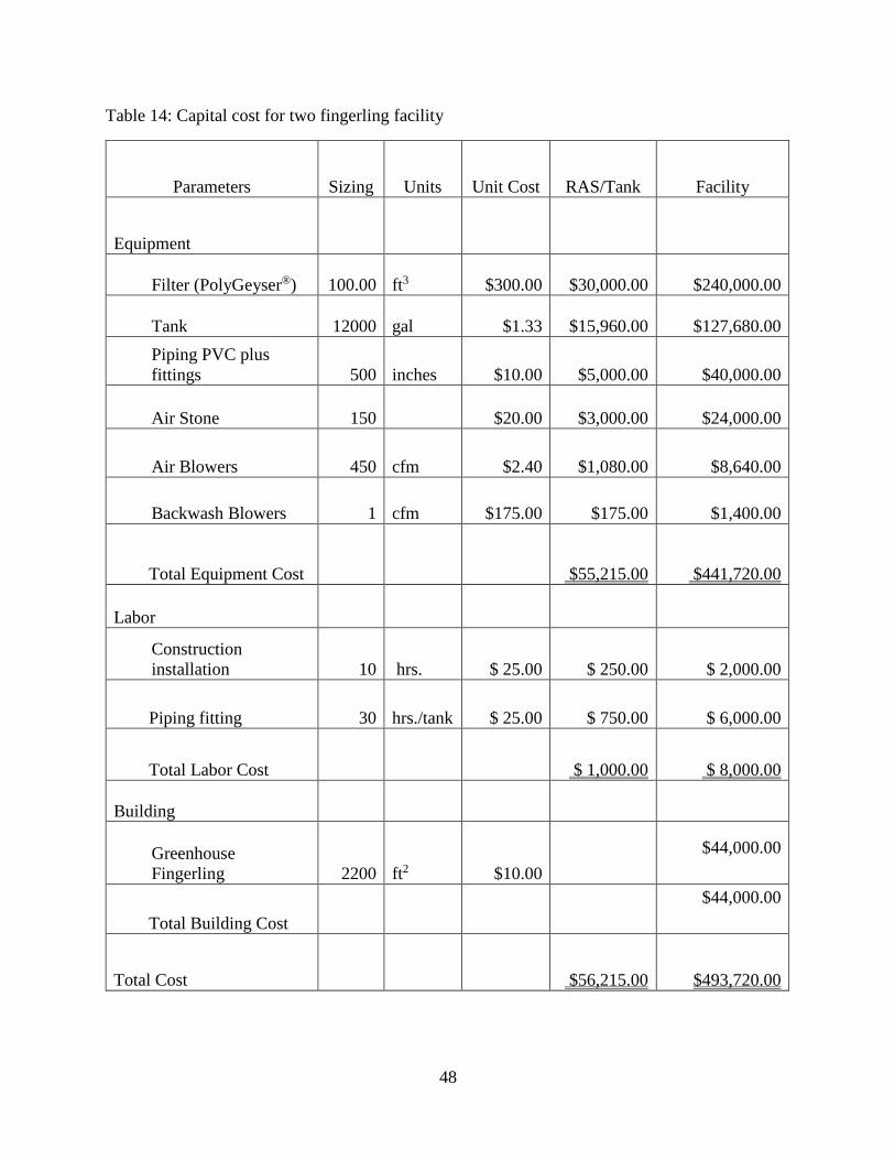
48
Table 14: Capital cost for two fingerling facility
Parameters Sizing Units Unit Cost RAS/Tank Facility
Equipment
Filter (PolyGeyser®) 100.00 ft3 $300.00 $30,000.00 $240,000.00
Tank 12000 gal $1.33 $15,960.00 $127,680.00
Piping PVC plus
fittings 500 inches $10.00 $5,000.00 $40,000.00
Air Stone 150 $20.00 $3,000.00 $24,000.00
Air Blowers 450 cfm $2.40 $1,080.00 $8,640.00
Backwash Blowers 1 cfm $175.00 $175.00 $1,400.00
Total Equipment Cost $55,215.00 $441,720.00
Labor
Construction
installation 10 hrs. $ 25.00 $ 250.00 $ 2,000.00
Piping fitting 30 hrs./tank $ 25.00 $ 750.00 $ 6,000.00
Total Labor Cost $ 1,000.00 $ 8,000.00
Building
Greenhouse
Fingerling 2200 ft2 $10.00
$44,000.00
Total Building Cost
$44,000.00
Total Cost $56,215.00 $493,720.00

49
Although fiberglass is not the cheapest material, it is one the most cost-effective and
reliable (Sprague, 1973; Howick et al., 1993). The fact that recirculation tanks are designed to self-
clean also reduces maintenance labor costs the construction installation (labor) and pipe fitting
requires 40 man hours with approximates cost of $8,000.00 for the fingerling section. Labor can
be completed by several workers simultaneously at a salary of $25.00/hr. Each tank is furnished
with two 50 ft³ PolyGeyser® filters at a unit cost of $12,000 for each tank. Each fingerling building
has 4 tanks, so the fingerling filter cost for the whole facility is $240,000. The air blowers, which
are determined to be set at 450 cfm with a unit cost $2.40 per cfm thus a total cost of $8,640. The
least expensive building material is the metallic greenhouse (market prices range from $10 to
40/ft², which is cheaper than conventional buildings). Material is needed for an area of 4400 ft²,
and we selected the lowest material cost of $10.00/ft². Thus, two fingerling building costs $44,000.
Fingerling production
The operational costs are obtained from expenses and management plans associated with
operation and maintenance. The target amount to farm is 1,029,800 pound of harvestable fish
divided into 8 initial fingerling tanks. Thus, each fingerling tank provides for 3 growout tanks
(with 24 growout tanks in the facility). The Table 15 details the operational expenditures associated
with annual fingerling production for each tank, each building, and for the entire facility.
As indicated in Table 15, each fingerling costs $0.16, based on a 5g fingerling weight. This
leads to an annual fingerling production cost at $0.52 per fingerling up to the 70g, based on the
design criteria. The stocking cost for the fingerling annual production is $106,500 for the entire
fingerling facility: feeding is $51,800/year, and chemical cost is $24,864 per year. The electricity,
labor, and heating annual costs for each tank are estimated at $69,277, $21,600, and $4,712.50,
respectfully. The miscellaneous cost is two percent of the overall fingerling cost.
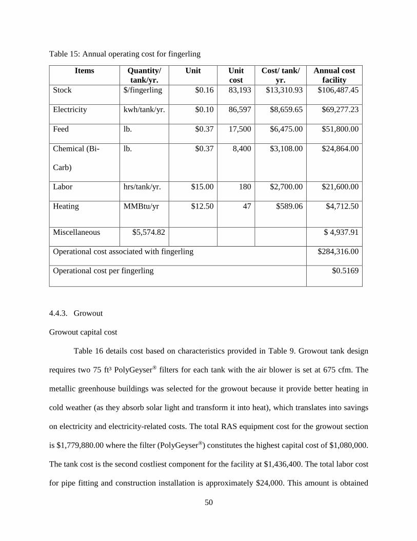
50
Table 15: Annual operating cost for fingerling
Items Quantity/
tank/yr.
Unit Unit
cost
Cost/ tank/
yr.
Annual cost
facility
Stock $/fingerling $0.16 83,193 $13,310.93 $106,487.45
Electricity kwh/tank/yr. $0.10 86,597 $8,659.65 $69,277.23
Feed lb. $0.37 17,500 $6,475.00 $51,800.00
Chemical (Bi-
Carb)
lb. $0.37 8,400 $3,108.00 $24,864.00
Labor hrs/tank/yr. $15.00 180 $2,700.00 $21,600.00
Heating MMBtu/yr $12.50 47 $589.06 $4,712.50
Miscellaneous $5,574.82 $ 4,937.91
Operational cost associated with fingerling $284,316.00
Operational cost per fingerling $0.5169
4.4.3. Growout
Growout capital cost
Table 16 details cost based on characteristics provided in Table 9. Growout tank design
requires two 75 ft³ PolyGeyser® filters for each tank with the air blower is set at 675 cfm. The
metallic greenhouse buildings was selected for the growout because it provide better heating in
cold weather (as they absorb solar light and transform it into heat), which translates into savings
on electricity and electricity-related costs. The total RAS equipment cost for the growout section
is $1,779,880.00 where the filter (PolyGeyser®) constitutes the highest capital cost of $1,080,000.
The tank cost is the second costliest component for the facility at $1,436,400. The total labor cost
for pipe fitting and construction installation is approximately $24,000. This amount is obtained
51
based on a total of forty man hours at a salary of $25.00. To accommodate the four 45,000 gallon
tanks for each growout building, the facility needs a 6,200 ft2 area. Given a price of $10.00 per ft2,
the resulting total cost is $372,000 for the six growout buildings.
Growout production
As indicated in Table 17, annual production costs for the growout section of the facility
amount to $953,140. Figure 11 is a complementary bar chart that details the distribution of annual
growout production costs. Both include the stocking (fingerling) unit cost based on the production
cost to reach 70g per fingerling for transfer into growout tanks. This leads to a total growout facility
cost of $106,500. The feeding cost is the highest of the growout production at $496,200 which
consist of both the fingerling and growout cost. The chemical and electric cost are $105,050 and
$111,000 respectively. A labor cost of $64,800 was established base on the facility design.
Transportation estimations in Table 17 constitute the lesser cost. This amount was estimated at the
maximum rates, which means that in practice, transportation could be even less costly. In this
analysis, a food conversion ratio of 1.4 was assumed (1.4 lb. of feeding per lb. of fish produced).
Cost of feed was assumed at $0.37/lb. (about $0.13/lb. of fish produced).
The bi-carbonate is the same chemical as the one used for fingerlings, priced at $0.37/lb.,
that is, $105,050 annually for the facility. Results indicate that the proposed facility produces
1,029,800 lbs. of tilapia every year. Fingerling and growout cycles result in total production cost
of $0.93 /fish. The equipment production cost is $0.26 plus the purge facility production cost at
$0.01 gives an overall cost per lb. of fish at $1.19.
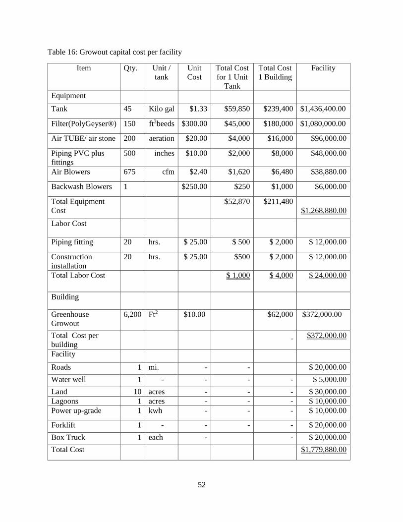
52
Table 16: Growout capital cost per facility
Item Qty. Unit /
tank
Unit
Cost
Total Cost
for 1 Unit
Tank
Total Cost
1 Building
Facility
Equipment
Tank 45 Kilo gal $1.33 $59,850 $239,400 $1,436,400.00
Filter(PolyGeyser®) 150 ft3beeds $300.00 $45,000 $180,000 $1,080,000.00
Air TUBE/ air stone 200 aeration $20.00 $4,000 $16,000 $96,000.00
Piping PVC plus
fittings
500 inches $10.00 $2,000 $8,000 $48,000.00
Air Blowers 675 cfm $2.40 $1,620 $6,480 $38,880.00
Backwash Blowers 1 $250.00 $250 $1,000 $6,000.00
Total Equipment
Cost
$52,870 $211,480
$1,268,880.00
Labor Cost
Piping fitting 20 hrs. $ 25.00 $ 500 $ 2,000 $ 12,000.00
Construction
installation
20 hrs. $ 25.00 $500 $ 2,000 $ 12,000.00
Total Labor Cost $ 1,000 $ 4,000 $ 24,000.00
Building
Greenhouse
Growout
6,200 Ft2 $10.00 $62,000 $372,000.00
Total Cost per
building
$372,000.00
Facility
Roads 1 mi. - - $ 20,000.00
Water well 1 - - - - $ 5,000.00
Land 10 acres - - - $ 30,000.00
Lagoons 1 acres - - - $ 10,000.00
Power up-grade 1 kwh - - - $ 10,000.00
Forklift 1 - - - - $ 20,000.00
Box Truck 1 each - - $ 20,000.00
Total Cost $1,779,880.00
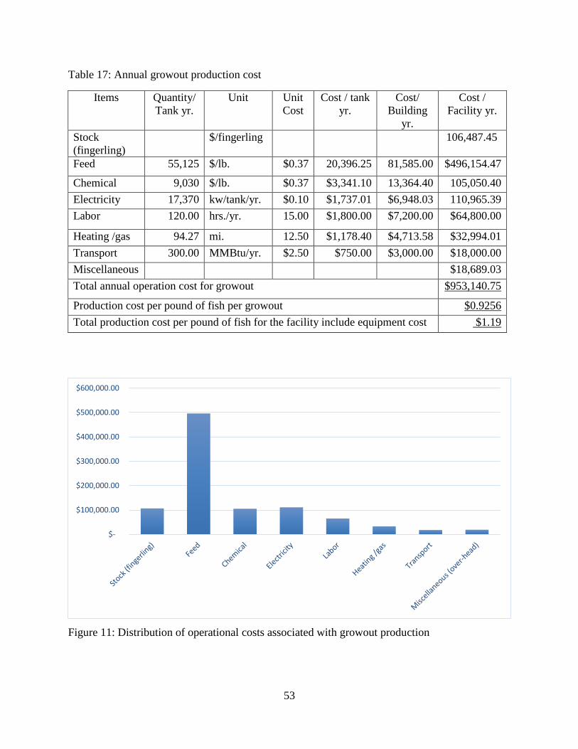
53
Table 17: Annual growout production cost
Items Quantity/
Tank yr.
Unit Unit
Cost
Cost / tank
yr.
Cost/
Building
yr.
Cost /
Facility yr.
Stock
(fingerling)
$/fingerling 106,487.45
Feed 55,125 $/lb. $0.37 20,396.25 81,585.00 $496,154.47
Chemical 9,030 $/lb. $0.37 $3,341.10 13,364.40 105,050.40
Electricity 17,370 kw/tank/yr. $0.10 $1,737.01 $6,948.03 110,965.39
Labor 120.00 hrs./yr. 15.00 $1,800.00 $7,200.00 $64,800.00
Heating /gas 94.27 mi. 12.50 $1,178.40 $4,713.58 $32,994.01
Transport 300.00 MMBtu/yr. $2.50 $750.00 $3,000.00 $18,000.00
Miscellaneous $18,689.03
Total annual operation cost for growout $953,140.75
Production cost per pound of fish per growout $0.9256
Total production cost per pound of fish for the facility include equipment cost $1.19
Figure 11: Distribution of operational costs associated with growout production
$-
$100,000.00
$200,000.00
$300,000.00
$400,000.00
$500,000.00
$600,000.00
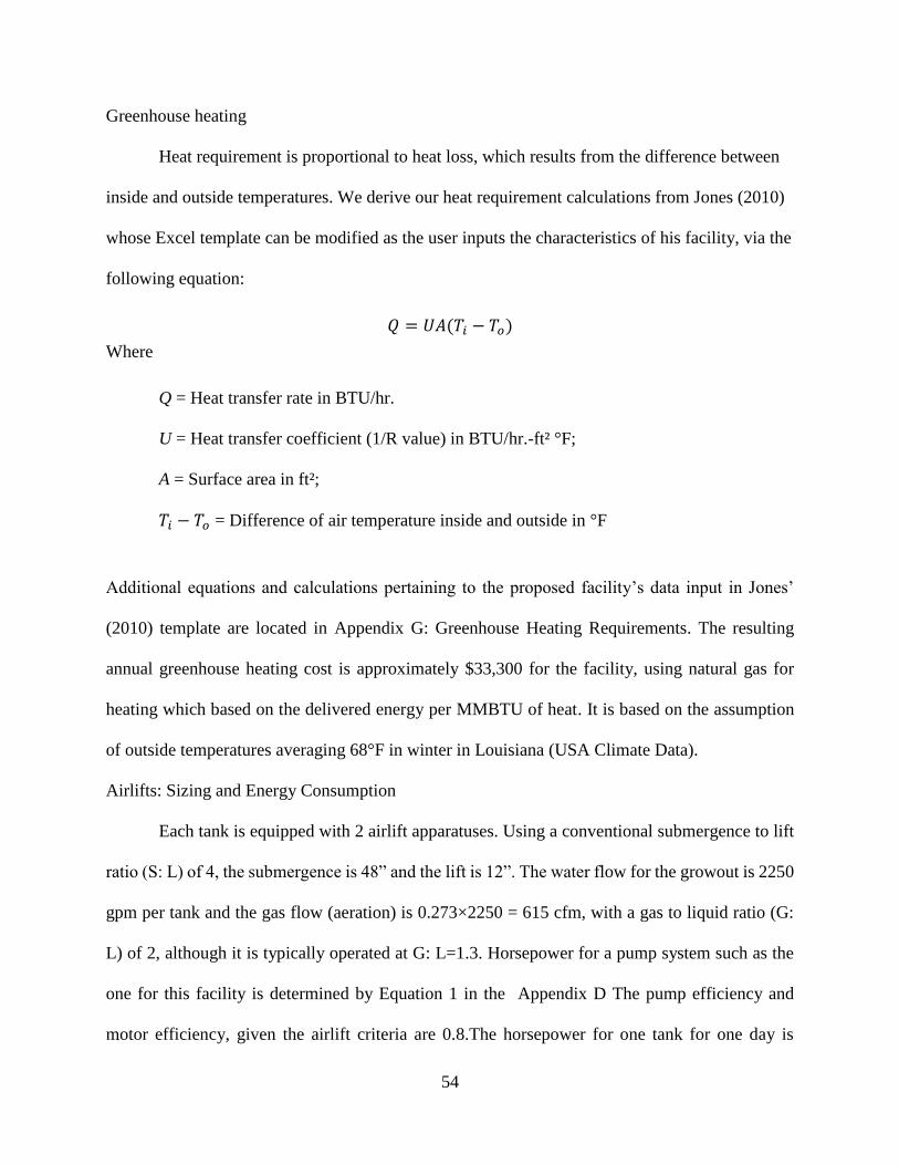
54
Greenhouse heating
Heat requirement is proportional to heat loss, which results from the difference between
inside and outside temperatures. We derive our heat requirement calculations from Jones (2010)
whose Excel template can be modified as the user inputs the characteristics of his facility, via the
following equation:
𝑄 = 𝑈𝐴(𝑇𝑖 − 𝑇𝑜)
Where
Q = Heat transfer rate in BTU/hr.
U = Heat transfer coefficient (1/R value) in BTU/hr.-ft² °F;
A = Surface area in ft²;
𝑇𝑖 − 𝑇𝑜 = Difference of air temperature inside and outside in °F
Additional equations and calculations pertaining to the proposed facility’s data input in Jones’
(2010) template are located in Appendix G: Greenhouse Heating Requirements. The resulting
annual greenhouse heating cost is approximately $33,300 for the facility, using natural gas for
heating which based on the delivered energy per MMBTU of heat. It is based on the assumption
of outside temperatures averaging 68°F in winter in Louisiana (USA Climate Data).
Airlifts: Sizing and Energy Consumption
Each tank is equipped with 2 airlift apparatuses. Using a conventional submergence to lift
ratio (S: L) of 4, the submergence is 48” and the lift is 12”. The water flow for the growout is 2250
gpm per tank and the gas flow (aeration) is 0.273×2250 = 615 cfm, with a gas to liquid ratio (G:
L) of 2, although it is typically operated at G: L=1.3. Horsepower for a pump system such as the
one for this facility is determined by Equation 1 in the Appendix D The pump efficiency and
motor efficiency, given the airlift criteria are 0.8.The horsepower for one tank for one day is
55
therefore calculated, resulting in a value of 2.78 hp. The electric cost of airlift operation alone is
$41,688.16 per facility per year. Knowing that each tank yields 42,900 lbs. fish per tank per yr. of
fish upon completion of a cycle, the electricity cost is $0.10 per lb. of fish produced.
Overall labor
Regular supply of labor is required to ensure proper operation and maintenance. Thus three
employees are selected to operate the facility which gives a total annual salary of $69,300.00. This
don’t include the engineer worker or other overhead labor cost.
4.4.4. Purge Tanks
The purge building capital cost for one 15,000 gallon tank with a 50 ft3 bead filter
(PolyGeyser®). The total RAS cost of the purge building is $23,920. The building design to
accommodate the purge tank is 1,000 ft2 at a cost of $10,000. The construction installation and
piping fitting have a total cost of $1,000 thus a total capital cost of $33,920. Table 18 and Table
19 detail the costs associated with operation and capital.
Table 18: Annual operation costs for purge tanks
Items Quantity/
tank/yr.
Unit Unit cost Annual cost
facility
Electricity 21,649 kwh/tank/yr. $ 0.10 $ 2,164.91
Labor 300 hrs./tank/yr. $ 15.00 $ 4,500.00
Heating 24 MMBtu/yr. $ 12.50 $ 294.53
Miscellaneous $ 139.19
Total Cost $ 7,098.63
Production cost/lb. for purge tank $ 0.01
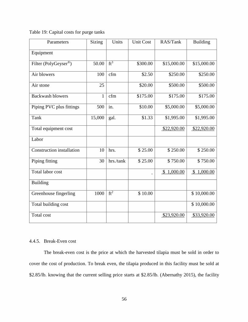
56
Table 19: Capital costs for purge tanks
Parameters Sizing Units Unit Cost RAS/Tank Building
Equipment
Filter (PolyGeyser®) 50.00 ft3 $300.00 $15,000.00 $15,000.00
Air blowers 100 cfm $2.50 $250.00 $250.00
Air stone 25 $20.00 $500.00 $500.00
Backwash blowers 1 cfm $175.00 $175.00 $175.00
Piping PVC plus fittings 500 in. $10.00 $5,000.00 $5,000.00
Tank 15,000 gal. $1.33 $1,995.00 $1,995.00
Total equipment cost $22,920.00 $22,920.00
Labor
Construction installation 10 hrs. $ 25.00 $ 250.00 $ 250.00
Piping fitting 30 hrs./tank $ 25.00 $ 750.00 $ 750.00
Total labor cost $ 1,000.00 $ 1,000.00
Building
Greenhouse fingerling 1000 ft2 $ 10.00 $ 10,000.00
Total building cost $ 10,000.00
Total cost $23,920.00 $33,920.00
4.4.5. Break-Even cost
The break-even cost is the price at which the harvested tilapia must be sold in order to
cover the cost of production. To break even, the tilapia produced in this facility must be sold at
$2.85/lb. knowing that the current selling price starts at $2.85/lb. (Abernathy 2015), the facility
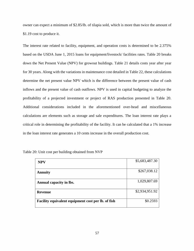
57
owner can expect a minimum of $2.85/lb. of tilapia sold, which is more than twice the amount of
$1.19 cost to produce it.
The interest rate related to facility, equipment, and operation costs is determined to be 2.375%
based on the USDA June 1, 2015 loans for equipment/livestock/ facilities rates. Table 20 breaks
down the Net Present Value (NPV) for growout buildings. Table 21 details costs year after year
for 30 years. Along with the variations in maintenance cost detailed in Table 22, these calculations
determine the net present value NPV which is the difference between the present value of cash
inflows and the present value of cash outflows. NPV is used in capital budgeting to analyze the
profitability of a projected investment or project of RAS production presented in Table 20.
Additional considerations included in the aforementioned over-head and miscellaneous
calculations are elements such as storage and sale expenditures. The loan interest rate plays a
critical role in determining the profitability of the facility. It can be calculated that a 1% increase
in the loan interest rate generates a 10 cents increase in the overall production cost.
Table 20: Unit cost per building obtained from NVP
NPV $5,683,487.30
Annuity $267,038.12
Annual capacity in lbs. 1,029,807.69
Revenue $2,934,951.92
Facility equivalent equipment cost per lb. of fish $0.2593
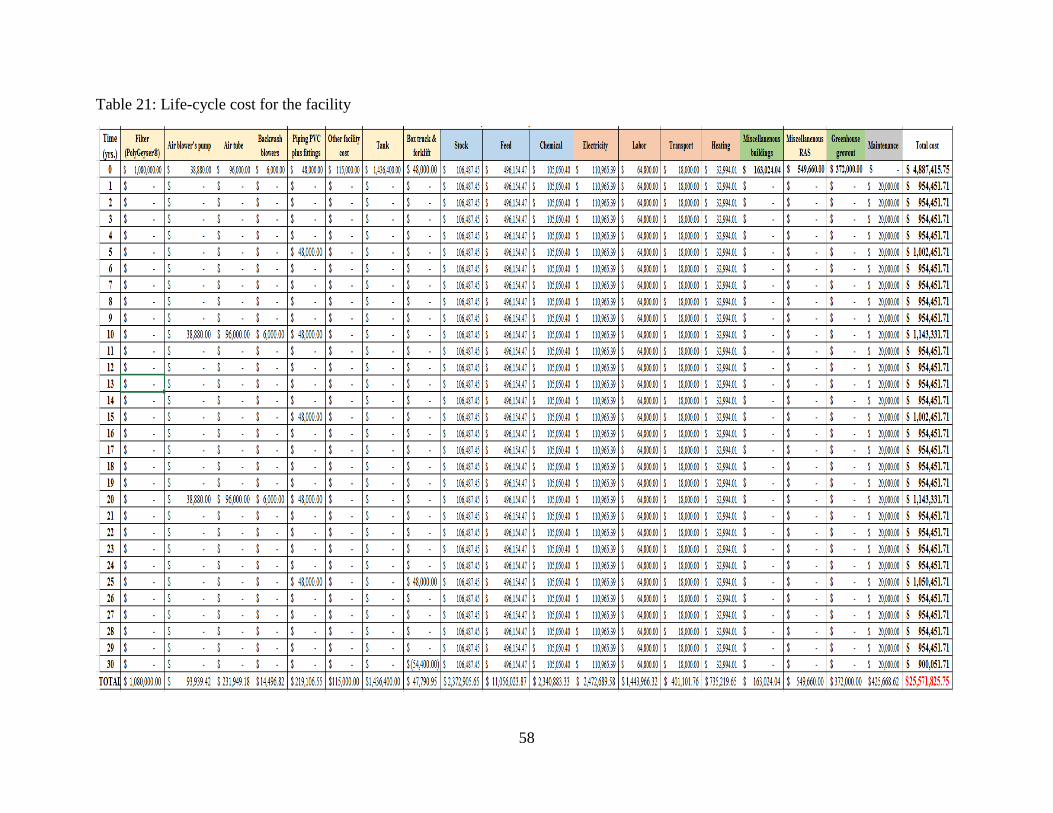
58
Table 21: Life-cycle cost for the facility
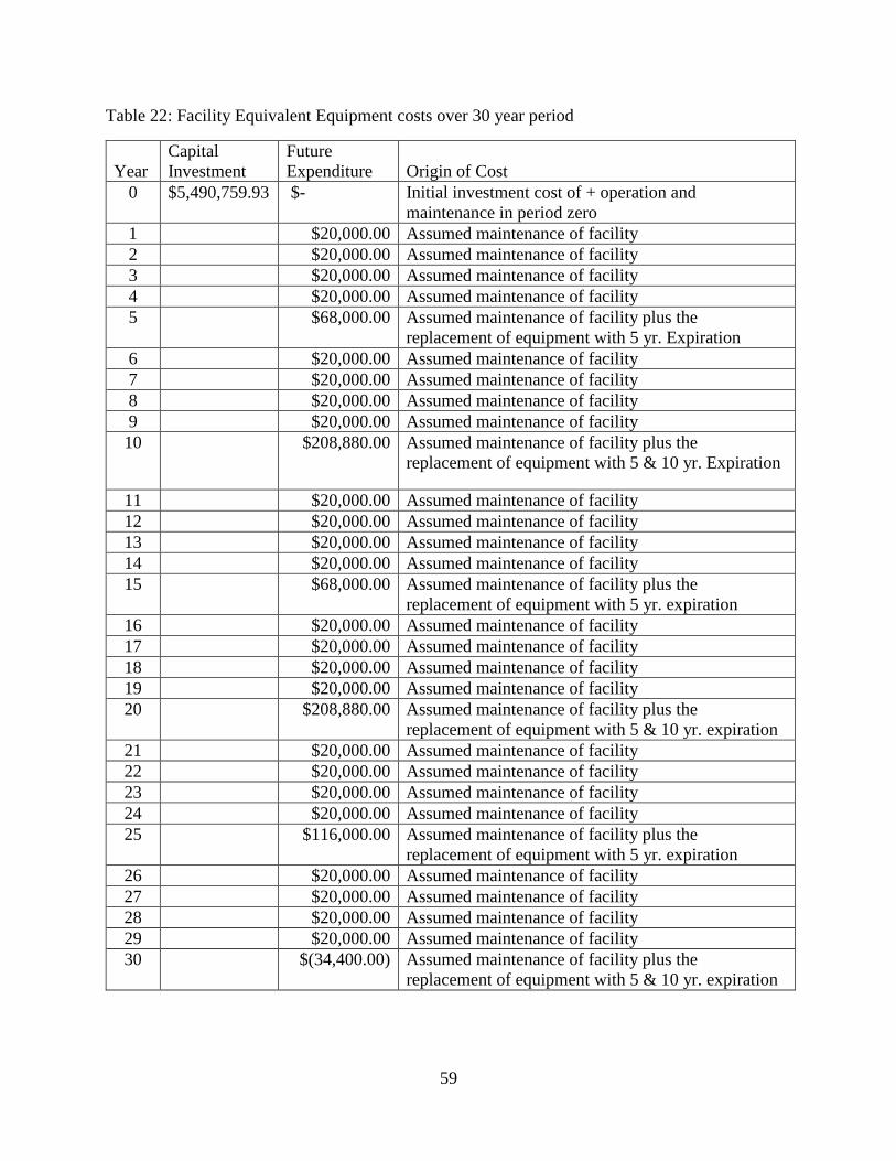
59
Table 22: Facility Equivalent Equipment costs over 30 year period
Year
Capital
Investment
Future
Expenditure Origin of Cost
0 $5,490,759.93 $- Initial investment cost of + operation and
maintenance in period zero
1 $20,000.00 Assumed maintenance of facility
2 $20,000.00 Assumed maintenance of facility
3 $20,000.00 Assumed maintenance of facility
4 $20,000.00 Assumed maintenance of facility
5 $68,000.00 Assumed maintenance of facility plus the
replacement of equipment with 5 yr. Expiration
6 $20,000.00 Assumed maintenance of facility
7 $20,000.00 Assumed maintenance of facility
8 $20,000.00 Assumed maintenance of facility
9 $20,000.00 Assumed maintenance of facility
10 $208,880.00 Assumed maintenance of facility plus the
replacement of equipment with 5 & 10 yr. Expiration
11 $20,000.00 Assumed maintenance of facility
12 $20,000.00 Assumed maintenance of facility
13 $20,000.00 Assumed maintenance of facility
14 $20,000.00 Assumed maintenance of facility
15 $68,000.00 Assumed maintenance of facility plus the
replacement of equipment with 5 yr. expiration
16 $20,000.00 Assumed maintenance of facility
17 $20,000.00 Assumed maintenance of facility
18 $20,000.00 Assumed maintenance of facility
19 $20,000.00 Assumed maintenance of facility
20 $208,880.00 Assumed maintenance of facility plus the
replacement of equipment with 5 & 10 yr. expiration
21 $20,000.00 Assumed maintenance of facility
22 $20,000.00 Assumed maintenance of facility
23 $20,000.00 Assumed maintenance of facility
24 $20,000.00 Assumed maintenance of facility
25 $116,000.00 Assumed maintenance of facility plus the
replacement of equipment with 5 yr. expiration
26 $20,000.00 Assumed maintenance of facility
27 $20,000.00 Assumed maintenance of facility
28 $20,000.00 Assumed maintenance of facility
29 $20,000.00 Assumed maintenance of facility
30 $(34,400.00) Assumed maintenance of facility plus the
replacement of equipment with 5 & 10 yr. expiration
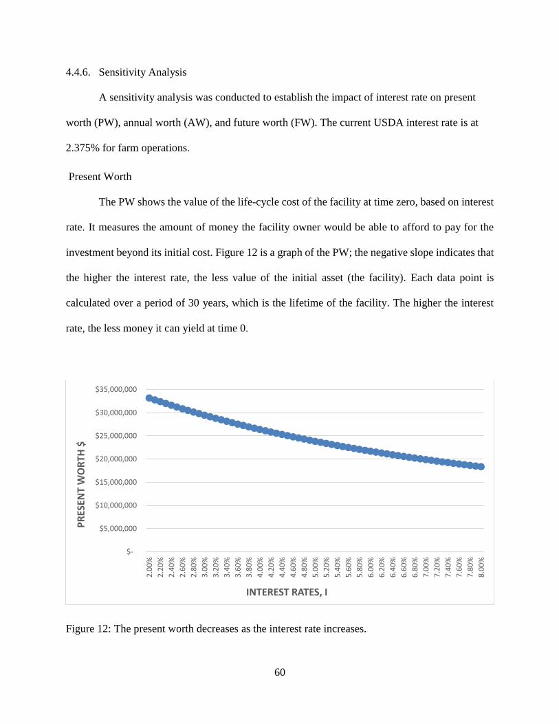
60
4.4.6. Sensitivity Analysis
A sensitivity analysis was conducted to establish the impact of interest rate on present
worth (PW), annual worth (AW), and future worth (FW). The current USDA interest rate is at
2.375% for farm operations.
Present Worth
The PW shows the value of the life-cycle cost of the facility at time zero, based on interest
rate. It measures the amount of money the facility owner would be able to afford to pay for the
investment beyond its initial cost. Figure 12 is a graph of the PW; the negative slope indicates that
the higher the interest rate, the less value of the initial asset (the facility). Each data point is
calculated over a period of 30 years, which is the lifetime of the facility. The higher the interest
rate, the less money it can yield at time 0.
Figure 12: The present worth decreases as the interest rate increases.
$-
$5,000,000
$10,000,000
$15,000,000
$20,000,000
$25,000,000
$30,000,000
$35,000,000
2.0
0%
2.2
0%
2.4
0%
2.6
0%
2.8
0%
3.0
0%
3.2
0%
3.4
0%
3.6
0%
3.8
0%
4.0
0%
4.2
0%
4.4
0%
4.6
0%
4.8
0%
5.0
0%
5.2
0%
5.4
0%
5.6
0%
5.8
0%
6.0
0%
6.2
0%
6.4
0%
6.6
0%
6.8
0%
7.0
0%
7.2
0%
7.4
0%
7.6
0%
7.8
0%
8.0
0%
PR
ESEN
T W
OR
TH $
INTEREST RATES, I

61
Annual Worth
The AW is calculated as the PW at increasing interest rate at period t. It is calculated as
the product of PW and capital recovery, which is the annual amount needed to cover loss in the
asset’s value and the interest in invested capital (Sullivan et al., 2003). Figure 13 shows that an
increase in interest rate is associated with an increase in AW. Sullivan et al. (2003) explained
that “as long as the AW is greater than or equal to zero, the project is economically attractive.”
Therefore, even with an increased interest rate and subsequent decreased PW, the facility
remains a very lucrative proposition. This is better for the lender; the higher the interest rate, the
more the borrower has to pay.
Figure 13: The annual worth increases as interest rate increases.
$1,400,000
$1,450,000
$1,500,000
$1,550,000
$1,600,000
$1,650,000
2.0
0%
2.2
0%
2.4
0%
2.6
0%
2.8
0%
3.0
0%
3.2
0%
3.4
0%
3.6
0%
3.8
0%
4.0
0%
4.2
0%
4.4
0%
4.6
0%
4.8
0%
5.0
0%
5.2
0%
5.4
0%
5.6
0%
5.8
0%
6.0
0%
6.2
0%
6.4
0%
6.6
0%
6.8
0%
7.0
0%
7.2
0%
7.4
0%
7.6
0%
7.8
0%
8.0
0%
AN
NU
AL
WO
RTH
$
INTEREST RATES, I

62
Future Worth
The FW is calculated as the product of AW and the uniform series compound amount factor
provided in The above equations from Oregon State University Energy Efficiency Reference
(2014) show the application of the heat requirement calculations in a sample automatic, computer-
generated professional report.
Appendix H: Sensitivity Analysis Formulae. Figure 14 indicates the extent to which the
facility’s future worth increases as the interest rate increases. For a project to be economically
justified, it must be more than or equal to zero. Figure 14 shows that even with higher interest
rates, the tilapia production facility remains not only viable, but profitable. The cash flow for the
borrower will be higher and the borrower will pay more. The lower the rate is better for the
borrower, the higher is better for the lender. If the rate is higher, the capital will be less.
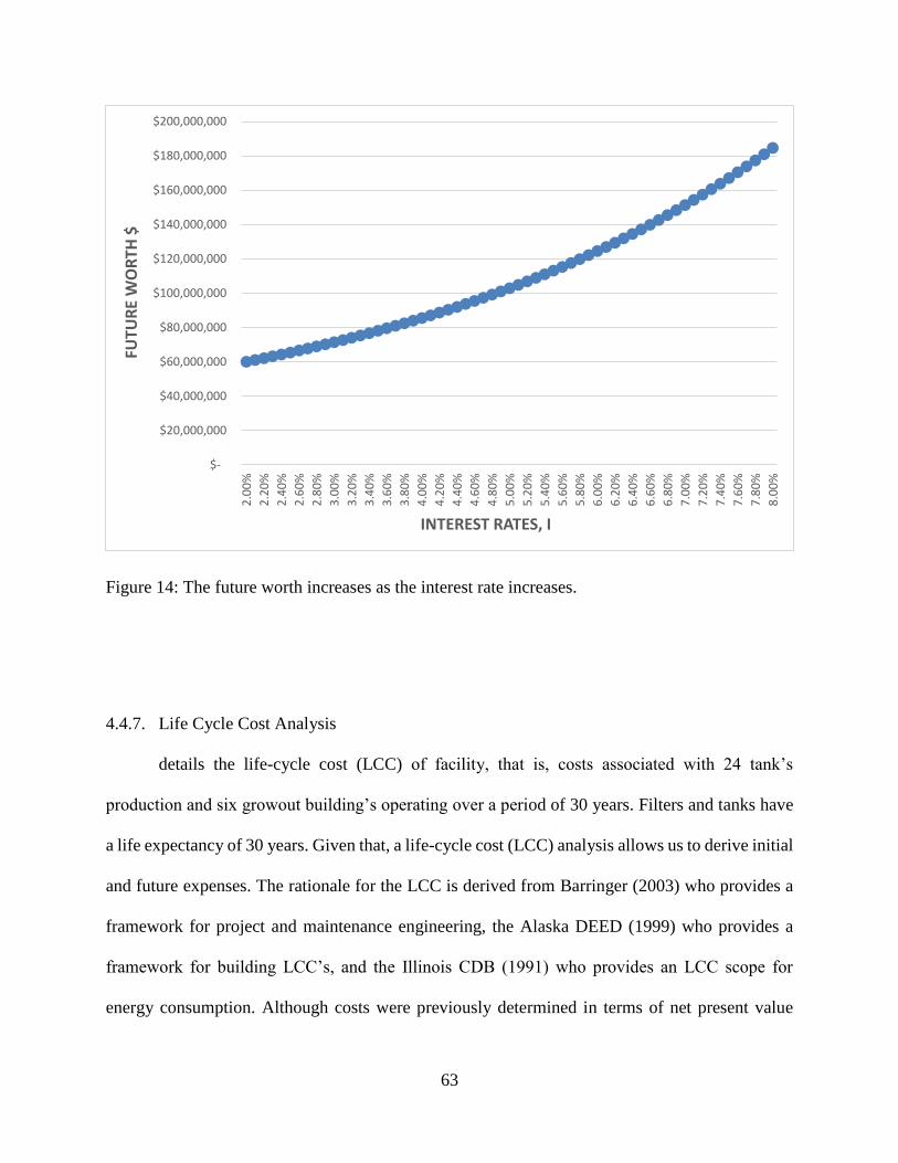
63
Figure 14: The future worth increases as the interest rate increases.
4.4.7. Life Cycle Cost Analysis
details the life-cycle cost (LCC) of facility, that is, costs associated with 24 tank’s
production and six growout building’s operating over a period of 30 years. Filters and tanks have
a life expectancy of 30 years. Given that, a life-cycle cost (LCC) analysis allows us to derive initial
and future expenses. The rationale for the LCC is derived from Barringer (2003) who provides a
framework for project and maintenance engineering, the Alaska DEED (1999) who provides a
framework for building LCC’s, and the Illinois CDB (1991) who provides an LCC scope for
energy consumption. Although costs were previously determined in terms of net present value
$-
$20,000,000
$40,000,000
$60,000,000
$80,000,000
$100,000,000
$120,000,000
$140,000,000
$160,000,000
$180,000,000
$200,000,000
2.0
0%
2.2
0%
2.4
0%
2.6
0%
2.8
0%
3.0
0%
3.2
0%
3.4
0%
3.6
0%
3.8
0%
4.0
0%
4.2
0%
4.4
0%
4.6
0%
4.8
0%
5.0
0%
5.2
0%
5.4
0%
5.6
0%
5.8
0%
6.0
0%
6.2
0%
6.4
0%
6.6
0%
6.8
0%
7.0
0%
7.2
0%
7.4
0%
7.6
0%
7.8
0%
8.0
0%
FUTU
RE
WO
RTH
$
INTEREST RATES, I
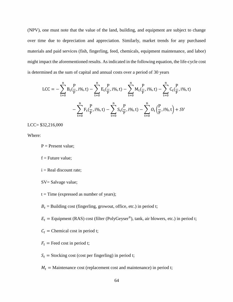
64
(NPV), one must note that the value of the land, building, and equipment are subject to change
over time due to depreciation and appreciation. Similarly, market trends for any purchased
materials and paid services (fish, fingerling, feed, chemicals, equipment maintenance, and labor)
might impact the aforementioned results. As indicated in the following equation, the life-cycle cost
is determined as the sum of capital and annual costs over a period of 30 years
LCC = − ∑ Bt(P
F, i%, t)
n
t=0
− ∑ Et(P
F, i%, t)
n
t=0
− ∑ Mt(P
F, i%, t)
n
t=0
− ∑ Ct(P
F, i%, t)
n
t=0
− ∑ Ft(P
F, i%, t)
n
t=0
− ∑ St(P
F, i%, t)
n
t=0
− ∑ 𝑂t (P
F, i%, t) + 𝑆𝑉
n
t=0
LCC= $32,216,000
Where:
P = Present value;
f = Future value;
i = Real discount rate;
SV= Salvage value;
t = Time (expressed as number of years);
𝐵𝑡 = Building cost (fingerling, growout, office, etc.) in period t;
𝐸𝑡 = Equipment (RAS) cost (filter (PolyGeyser®), tank, air blowers, etc.) in period t;
𝐶𝑡 = Chemical cost in period t;
𝐹𝑡 = Feed cost in period t;
𝑆𝑡 = Stocking cost (cost per fingerling) in period t;
𝑀𝑡 = Maintenance cost (replacement cost and maintenance) in period t;
65
𝑂𝑡 = Operation cost (labor, transportation, heating...etc.) in period t
Based on the 2014 USDA data, agriculture loans are set at a typical rate of 2.375%. The life cycle
cost of the proposed facility was therefore calculated to be $32,216,000. Figure 15 shows the
distribution of the major cost of the facility on a pie chart over the period (t) of 30 years.
The consumable cost, which includes the stocking, feeding and chemical cost, is
$15,800,000 at 62 percent of the entire life cycle cost in which the feeding cost is a little over
$11,056,000. The stocking cost is the second highest at $2,373,000 and the chemical is third part
of the consumable cost at $2,341,000.00 and the fifth highest among the LCC. The operation cost
and equipment cost is the third and fourth highest at $5,053,000 and $3,788,000. The building, and
maintenance cost follows at $535,000, and $426,000.
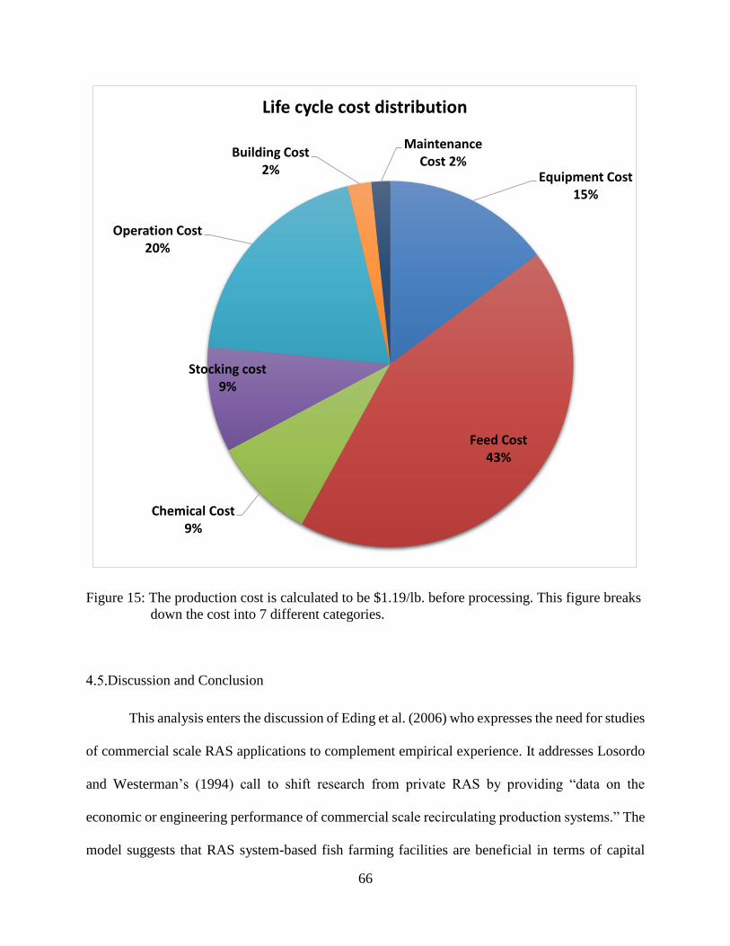
66
Figure 15: The production cost is calculated to be $1.19/lb. before processing. This figure breaks
down the cost into 7 different categories.
Discussion and Conclusion
This analysis enters the discussion of Eding et al. (2006) who expresses the need for studies
of commercial scale RAS applications to complement empirical experience. It addresses Losordo
and Westerman’s (1994) call to shift research from private RAS by providing “data on the
economic or engineering performance of commercial scale recirculating production systems.” The
model suggests that RAS system-based fish farming facilities are beneficial in terms of capital
Equipment Cost15%
Feed Cost43%
Chemical Cost9%
Stocking cost9%
Operation Cost20%
Building Cost2%
Maintenance Cost 2%
Life cycle cost distribution

67
costs, based on the facility size and the related parameters and components. This project thus
constitutes a step toward the process required to proceed to large scale tilapia production. It shows
the financial feasibility of intensive practice, and sets an example for budget templates and
decision-making tools for potential business undertakers.
The cost analysis sets the unit cost, as per the NPV, to produce one fish at approximately
$2.25 per kg. This cost is still higher than the cost for tilapia sold from China, which was priced at
$1.56/kg in 2013 (Tallaksen, 2013). Nonetheless, this study comes at a time when China’s tilapia
supply is decreasing as a result of the virus outbreak that affected the country’s poultry and swine
industries. Consequently, Chinese tilapia prices are on the rise (Stewart, 2013), which makes
domestic production even more competitive.
The proposed facility has a considerable margin of safety and room for production increase.
The filter runs at a very low density loading. Thus, an alternative management plan could involve
the formation of tilapia generation pools, or cohorts, or a cross-flow system. These alternative set-
ups would increase production significantly and would remarkably help save electricity-related
costs. The cohort system refers to having different sized fish staggering. This alternative plan is
detailed in Appendix E: Optional cohort design criteria. A cross-flow system involves different
tanks running into each other. Cohort and cross-flow systems can help increase production up to
30% for the facility. Nevertheless, the cross-flow system is a gamble in the sense that any
contagious disease emerging into the tank is destructive for the whole building or facility. Future
work, such as the research and calculations of Alt (2015) could help determine proportionality
between safety factor and cohort management variables. Evidently, the risk of fish disease is
present in this proposed facility as well, but the separate tanks and buildings it features help

68
mitigate the consequences of an outbreak. Another risk to consider is the constant possibility of
human error, particularly with chemical and feeding dosage.
A weakness of the proposed facility is that despite the fact that the RAS provides for a
smaller capital cost, substantial profit relies on managing the system well at decrease in market
prices or in demand would make it hard to break even. It would only exacerbate the threat of
competition and large-scale imports that is already hindering domestic tilapia production.
Consequently, fluctuations of the cost of feeding and electricity would affect its ability to subsist.
In addition, the system does not offer much room for detailed and considerably specific
improvement research, since key equipment (filters, blowers, etc.) comes in fixed-size and fixed-
capacity sets (they are classified in size, efficiency, and capacity ranges, not with custom-built
features).
It has already been established that RAS lower water demands and feed-generated wastes.
The recommended follow-up to this study would be a planning stage (Helfrich and Garling, 2009).
Such planning is potentially quite exhaustive since so many different biological, economic, and
legal factors must be taken into consideration. Gutierrez-Wing and Malone (2006) who present
future trends in RAS production explain that future research should “define the cost-
competitiveness of growout facilities.”
This next step should also include comparisons with other tilapia production facilities to
assess how beneficial the proposed facility has the potential to be. For instance, the facility
proposed in this thesis is capable of producing 1,053,500 lbs. of tilapia annually. Yet,
aquaculturists classify different growout system sizes and harvest amounts, designated as
-small system: <1,000,000 lbs. harvested yearly
-medium system: 1,000,000-5,000,000 lbs. harvested yearly
69
-large system: 5,000,000 lbs. and above harvested yearly (Malone, 2015)
At this point, the analyzed facility relates to the small system category. Evidently, the amount
produced via Airlifted PolyGeyser® RAS has great potential in comparison to the massive
production systems in China mentioned in Section 4.2. Increasing production size will allow the
production capabilities to exceed the massive import requirements of tilapia in America. In
conclusion, Airlifted PolyGeyser® RAS technology is an innovative way of meeting the demand
here at home and supply for future exports.
70
5. Conclusion
This thesis dealt with the three major aspects of aquaculture production systems for
monocultures, as defined in RUFORUM (2011): cultured species, culture facility, and husbandry.
Centered on airlift assisted RAS, it expanded from species-specific water quality management to
intensification, that is, “producing more fish with less water, less food, and less time to lower
production costs and reduce pollutants to the environment” (Watanabe et al., 2002). The two
studies examined the tank filtration need and the cost of aquaculture production
Airlifted RAS have the advantage of providing a more controlled environment for the
cultured species. Indeed, as RAS are acknowledged for their biosecurity, airlifts help maintain
proper pH and degasification. Biofilter-equipped RAS address environmental concerns mentioned
buy aqua-culturists and environmentalists: water quality, quantity, and discharge limitations, as
well as pollution (Gutierrez-Wing and Malone, 2006). Nevertheless, biosecurity needs vary
depending not only on the species cultured, but also its developmental stage. The egg loading data
collected in this thesis is useful in hatchery RAS design. We recommend further studies on water
quality at the larval stage.
Similarly, RAS production management unto the growout level differs from species to
species. Data obtained on numerous variables to determine the cost of tilapia production is
applicable to other species. One could also use the Chapter 3 (egg loading data) and Chapter 4’s
cost analysis to establish sizing criteria for the increasing demand for oligotrophic marine nurseries
and growout tanks and facilities by extension (Gutierrez-Wing and Malone, 2006).
Although the majority of Latin America and Caribbean tilapia producers utilize pond
systems, RAS are increasingly competing with ponds in the U.S. Large-scale commercial farming
is indeed a growing trend. As U.S. and world population and per capita seafood consumption grow,
71
the demand for large-scale aquaculture is intensified. This thesis’ cost analysis concludes that RAS
can be cost-efficient, although no conclusions were drawn on fish quality upon growout with RAS
v. ponds. Yet, Helfrich and Libey’s (1991) observations indicated that better fish taste may
translate into higher demand for RAS-produced tilapia, which could generate higher profit for
domestic industries.
The cost of RAS production can be expected to decrease in the future, not so much because
of investment cost, but rather because of the continual research and refinement of treatment
technology. In effect, contemporary aquacultural engineering seeks to produce more energy
efficient devices, and fishery and marine studies seek to produce feed with better feed conversion
ratios. These two variables have the largest impact on fish production, and are key to reducing
production cost.
From a long-range perspective, this study provides the background work and technical tool
required for the commercial aquaculture of different species in corresponding facilities, as it
contributes to determining the financial and biologic feasibility of such a trade. Indeed, Helfrich
and Garling (1985) explained that commercial aquaculture is completed in four major stages. First,
the planning stage constitutes the preliminary research to check the economic and biologic
feasibility of the project and to examine any legal constraints. Then, the training stage involves
water management and fish biology and culture. The training stage is followed by small scale
production and commercialization, including one or several pilot tests. Eventually, upon successful
completion of the third stage, commercial operation can take place.
Although this thesis does not mirror Helfrich and Garling’s (1985) entire plan, it
encompasses several of the items they mention. Indeed, the egg loading study examines biological
characteristics of decaying eggs and water management of biofouled water. Fahandezhsadi (2014)
72
provides a complementary framework. Her report provides a mathematical model that shows the
exponential growth of bacteria as hatchery water undergoes TAN biofouling. Furthermore, the
comparative data across species acquired in Chapter 3 provides a framework for egg substitution,
whereby studies on scarce, endangered, or expensive species can be conducted on more common
and affordable species that display similar loading characteristics. Substitution, along with the use
of heterotrophic bacteria acclimation (Fahandezhsadi, 2014) may help reduce the cost of bead-
only filters.
The corresponding filter requirement data is useable for small scale production. On the
other hand, the cost analysis provides a cost estimation framework for small and larger scale
production.
The use of RAS and PolyGeysers® for commercial scale aquaculture demands a
meticulously designed layout. Yet, building costs associated with construction can be avoided.
Utilizing existing buildings eliminates a significant portion of construction costs. The facility
should be equipped with a water source. Thus, the major parts of the equipment installation are to
take place in the interior of the building. The layout we have considered in this thesis is in
alignment with the recent simplified set of rules established to ensure optimal performance
regarding PolyGeyser®/Airlifts and similar filtration equipment (Malone and Gudipati, 2005).
As we have demonstrated, the most essential factors to be determined when elaborating a
cost analysis pertain to management, that is, the steps to take to proceed to and maintain production
once the physical characteristics criteria have been met. Therefore the management plan detailed
in Section 4.3.3 presents the different parameters to consider and the cost associated with them.
Future cost analyses should include and prioritize a similar table, adapting and modifying the initial
constants.

73
Figure 16: Distribution of operation costs for the proposed facility
Based on the LCC calculations the distribution of the operation cost shows the feeding and
stocking contribute 57 percent of the entire operation cost. This is a noteworthy fact because feed
cost is one of the reasons why the price of Chinese tilapia has been on the rise since the viral
contamination that affected the Chinese swine and poultry industries (Stewart, 2013).
Labor represents a significant portion of the facility’s operation costs. It is one of the main
reasons why domestically produced tilapia is overall more expensive than tilapia produced in Third
World countries from whom the U.S. imports the most. Indeed, the design set workers payment at
$25/hr. for construction installation and piping fitting with a minimum general labor wage of
$15/hr. Such a salary is not common practice in most Asian or South American fish production
facilities (FAO, 2014).
$-
$200,000.00
$400,000.00
$600,000.00
$800,000.00
$1,000,000.00
$1,200,000.00
$1,400,000.00
$1,600,000.00
$1,800,000.00
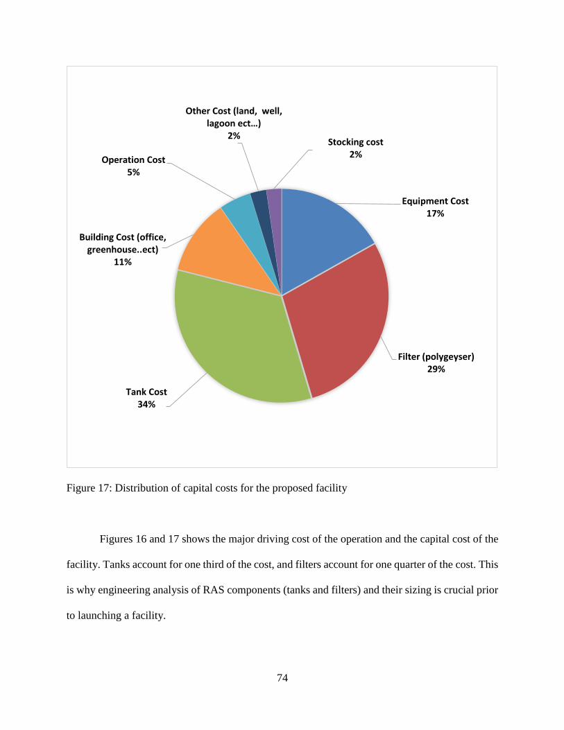
74
Figure 17: Distribution of capital costs for the proposed facility
Figures 16 and 17 shows the major driving cost of the operation and the capital cost of the
facility. Tanks account for one third of the cost, and filters account for one quarter of the cost. This
is why engineering analysis of RAS components (tanks and filters) and their sizing is crucial prior
to launching a facility.
Equipment Cost17%
Filter (polygeyser)29%
Tank Cost34%
Building Cost (office, greenhouse..ect)
11%
Operation Cost5%
Other Cost (land, well, lagoon ect…)
2%Stocking cost
2%
75
References
Abernathy, S. (2015). Personal interview. Arrowhead Fisheries. Canon City, CO.
Abdel-Hakim N.F.; Lashin, M.E.; Al-Azab A.A. and Nazmi, H.M. (2008). Effect of replacing
soybean meal protein by other plant protein sources on growth performance and economical
efficiency of mono sex Nile tilapia (Oreochromis niloticus) cultured in tankes.8th
International Sym. on Tilapia in Aqua.2008.739-744.
Alt, D. (2015) Mass balance analysis of load leveling techniques in recirculation aquaculture
systems Master’s thesis. Department of Civil and Environmental Engineering. Louisiana
State University. Baton Rouge, LA.
American Public Health Association. (1976). Standard Methods for the Examination of Water and
Wastewater 14ed. APHA.
Andrews, C. (1990). The ornamental fish trade and fish conservation. Journal of fish
Biology, 37(sA), 53-59.
Aquaculture Systems Technologies. (2006). Bead Filter Model DF-6. Updated Version-3
09/27/06.
Armstrong, J. D., Kemp, P. S., Kennedy, G. J. A., Ladle, M., and Milner, N. J. (2003). Habitat
requirements of Atlantic salmon and brown trout in rivers and streams. Fisheries
research, 62(2), 143-170.
Arthur, J. W., West, C. W., Allen, K. N., and Hedtke, S. F. (1987). Seasonal toxicity of ammonia
to five fish and nine invertebrate species. Bulletin of Environmental Contamination and
Toxicology, 38(2), 324-331.
Asian Institute of Technology. (1994). Partners in Development, the Promotion of Sustainable
Aquaculture. AIT, Bangkok.
Auld, A. H., and Schubel, J. R. (1978). Effects of suspended sediment on fish eggs and larvae: a
laboratory assessment. Estuarine and Coastal Marine Science, 6(2), 153-164.
Awari, G. K., Ardhapurkar, P. M., Wakde, D. G., and Bhuyar, L. B. (2004). Performance analysis
of air-lift pump design. Proceedings of the Institution of Mechanical Engineers, Part C:
Journal of Mechanical Engineering Science,218(10), 1155-1161.
Badiola, M., Mendiola, D., and Bostock, J. (2012). Recirculating Aquaculture Systems (RAS)
analysis: Main issues on management and future challenges. Aquacultural Engineering, 51,
26-35.
Ball, I. R. (1967). The relative susceptibilities of some species of fresh-water fish to poisons—I.
Ammonia. Water Research, 1(11), 767-775.
76
Barringer, H. P. (2003, May). A life cycle cost summary. In International Conference on
Maintenance Societies, Perth, Australia, May. 20-23.
Beem, M., and Hobbs, J. C. (1995). Recirculating Aquaculture Systems: Questions to Ask Before
you Invest. OSU extension facts (USA). no. F-9207.
Bellelo, S. M. (2006). Evaluation of Media Influence and Practical Applications for the Use of
Static Low Density Media Filters in Domestic Wastewater Treatment. M.S. Thesis.
Department of Civil and Environmental Engineering. Louisiana State University. Baton
Rouge, LA.
Bellido, J. M., Brown, A. M., Valvanis, V. D., Giraldez, A., Pierce G. J., Iglesias, M., and
Palialexis, A. (2008). Identifying Essential Fish Habitat for Small Pelagic Species in
Mediterranean Waters.
Berger, J. (1930). U.S. Patent No. 1,759,729. Washington, DC: U.S. Patent and Trademark Office.
Bergheim, A., Hustveit, H., Kittelsen, A., and Selmer-Olsen, A. R. 1984). (Estimated Pollution
Loadings from Norwegian Fish Farms. II. Investigations 1980–1981. Aquaculture: 36 (1-2).
157–168.
Blaxter, J. H. S. (1969). Development Eggs and Larvae. In W.S. Hoar, D.J. Randall (Eds.), Fish
physiology, 3. Academic Press, New York and London. 177–252.
Bocek, A. (2009). Water Harvesting and Aquaculture for Rural Development.International Center
for Aquaculture and Aquatic Environments, Swingle Hall. Auburn University Alabama,
36849-5419.
Boehlje, M. and C. Ehmke, 2005. Capital investment analysis and project assessment.
Metropolitan State College of Denver.
Bowser, P. R., Wooster, G. A., Getchell, R. G., and Timmons, M. B. (1998). Streptococcus Iniae
Infection of Tilapia Oreochromis Niloticus in a Recirculation Production Facility. Journal of
the World Aquaculture Society, 29(3), 335-339.
Braithwaite, R. A., Carrascosa, M. C. C., and McEvoy, L. A. (2007). Biofouling of Salmon Cage
Netting and the Efficacy of a Typical Copper-Based Antifoulant.Aquaculture, 262(2), 219-
226.
Braum, E. (1973). Einflüsse Chronischen Exogenen Sauerstoffmangels auf die Embryogenese des
Herings (Clupea harengus). Netherlands Journal of Sea Research, 7, 363-375.
Brindle, K., and Stephenson, T. (1996). The Application of Membrane Biological Reactors for the
Treatment of Wastewaters. Biotechnology and Bioengineering,49(6), 601-610.
Brown, C. L., Power, D. M., and Núñez, J. M. (2010). 5 Disorders of Development in Fish. Fish
Diseases and Disorders, 2, 166.
77
Bruckner A. W. (2005). The importance of the marine ornamental reef fish trade in the wider
Caribbean. NOAA Fisheries.
Bucker, B. B. (2014). Chapter 2. Climate of Louisiana. www.latech.edu/tech/liberal-
arts/geography/courses/310/text/climate.
Burden, D. (1988). Development and Design of a Fluidized Bed/Upflow Sand Filter Configuration
for Use in Recirculating Aquaculture Systems. Ph.D. Dissertation. Louisiana State
University. Department of Civil Engineering.
Burrows, R. E. (1964). Effects of accumulated excretory products on hatchery-reared salmonids.
Bureau of Sport Fisheries and Wildlife.
Carpenter, J. H. (1965a). The accuracy of the Winkler method for dissolved oxygen. Limnology
and Oceanography 10: 135-140.
Casebolt D. B., Spear D. J., Horney B. S. Care and Use of Fish as Laboratory Animals: Current
State of Knowledge. 1998.
Castilho, L.R., D.A. Mitchell, and D.M. Freire. (2009). Production of polyhydroxyalkanoates
(PHAs) from waste materials and by-products by submerged and solid-state fermentation.
Bioresource Technology, 100 (23), 5996-6009.
Chambers L. D., Stokes K. R., Walsh F. C., and Wood R. J. K. Modern approaches to marine
antifouling coatings. Surface and Coatings Technology: 201. 2006. 3642-3652.
Chanprateep, S. (2010). Current trends in biodegradable polyhydroxyalkanoates. Journal of
bioscience and bioengineering, 110(6), 621-632.
Chapman, P. W. (1980). U.S. Patent No. 4,212,268. Washington, DC: U.S. Patent and Trademark
Office.
Chapman, F. A., Fitz‐Coy, S. A., Thunberg, E. M., and Adams, C. M. (1997). United States of
America trade in ornamental fish. Journal of the World Aquaculture Society, 28(1), 1-10.
Chen, S., Coffin, D. E. and Malone, R. F. (1997). Sludge production and management for
recirculating aquacultural systems. Journal of the World Aquaculture Society, 28(4), 303-
315.
Chitta, B. S. (1993). Effects of backwash frequency on nitrification in plastic bead media biofilters
used in recirculating finfish culture systems (Doctoral dissertation, Louisiana State
University, Baton Rouge).
Choubert Jr, G., De La Noüe, J., and Luquet, P. (1979). Continuous quantitative automatic
collector for fish feces. The Progressive Fish-Culturist, 41(2), 64-67.
Choubert, G., De la Noüe, J., and Luquet, P. (1982). Digestibility in fish: improved device for the
automatic collection of feces. Aquaculture, 29(1), 185-189.

78
Church, B. D., Widmer, C. M. and Espinosa, R. (1977). Fungal conversion of carbohydrate wastes
to animal feed protein-vitamin supplements. In Proceedings, 8th National Symposium on
Food Processing Wastes, US Environmental Protection Agency, Washington, USA. 355-388.
Cook, F. J., Pankhurst, C. E. D Amato, C., Fanning, D. J., and Carlin, G. D. (2003). Effects of
trash incorporation and soil water content on the rate of breakdown of soluble sugars in the
soil following sugarcane harvest. In Proceedings, Australian Society of Sugar Cane
Technologists. PK Editorial Services; 1999. 9-9.
Copeland, K. A., Watanabe, W. O., and Dumas, C. E. (2005). Economic Evaluation of a Small‐Scale Recirculating System for Ongrowing of Captive Wild Black Sea Bass Centropristis
striata in North Carolina. Journal of the World Aquaculture Society, 36(4), 489-497.
Cronin, E. R., Cheshire, A. C., Clarke, S. M., and Melville, A. J. (1999). An investigation into the
composition, biomass and oxygen budget of the fouling community on a tuna aquaculture
farm. Biofouling, 13(4), 279-299.
d’Orbcastel, E. R., Blancheton, J. P., and Aubin, J. (2009). Towards environmentally sustainable
aquaculture: Comparison between two trout farming systems using Life Cycle
Assessment. Aquacultural Engineering, 40(3), 113-119.
Daykin, P. N. (1965). Application of mass transfer theory to the problem of respiration of fish
eggs. Journal of the Fisheries Board of Canada, 22(1), 159-171.
DeTolla, L. J., Srinivas, S., Whitaker, B. R., Andrews, C., Hecker, B., Kane, A. S., and
Reimschuessel, R. (1995). Guidelines for the care and use of fish in research. Ilar
Journal, 37(4), 159-173.
Diana, J. S., Lin, C. K., and Yi, Y. (1996). Timing of supplemental feeding for tilapia
production. Journal of the world aquaculture society, 27(4), 410-419.
Drennan, D. G., Hosler, K. C., Francis, M., Weaver, D., Aneshansley, E., Beckman, G., Johnson,
C. H. and Cristina, C. M. (2006). Standardized evaluation and rating of biofilters: II.
Manufacturer's and user's perspective. Aquacultural engineering, 34(3), 403-416.
Eding, E. H., Kamstra, A., Verreth, J. A. J., Huisman, E. A. and Klapwijk, A. (2006). Design and
operation of nitrifying trickling filters in recirculating aquaculture: a review. Aquacultural
Engineering, 34(3), 234-260.
El-Sayed, A. F. M. (2006). Tilapia culture. CABI Publishing, Cambridge, MA.
Fahandezhsadi, F. (2014). Assimilation, a Biological Nitrogen Removal Strategy for Freshwater
Ornamental Fish Hatcheries. Master’s thesis. Louisiana State University. Baton Rouge, LA.
FAO Fisheries and Aquaculture Department. (2011). Market reports: Tilapia August 2011. United
Nations.http://www.globefish.org/global-production-and-demand-for-tilapia-is-steady.html.

79
Fatone, F., Battistoni, P., Pavan, P., and Cecchi, F. (2007). Operation and maintenance of full-
scale municipal membrane biological reactors: A detailed overview on a case
study. Industrial and Engineering Chemistry Research, 46(21), 6688-6695.
Food and Agriculture Organization of the United Nations 2014 fao.org/3/a-i3720e.pdf
Finn, R. N., Fyhn, H. J., and Evjen, M. S. (1991). Respiration and nitrogen metabolism of Atlantic
halibut eggs (Hippoglossus hippoglossus). Marine Biology, 108(1), 11-19.
Fitzsimmons, K. (2000). Future trends of tilapia aquaculture in the Americas.Tilapia aquaculture
in the Americas, 2, 252-264.
Fitzsimmons, K. (2004, September). Development of new products and markets for the global
tilapia trade. In Proceeding of the Sixth International Symposium on Tilapia in Aquaculture,
Manila, Philippines (ed. By R. Bolivar, G. Mair and K. Fitzsimmons) pp (pp. 624-633).
Gabbadon, P., de Souza, G., and Titus, A. (1998; Revised Edition, 2008). Tilapia farming: A
manual for commercial tilapia production in Trinidad and Tobago. Institute of Marine
Affairs.
Georgia Cooperative Extension. (2014).
Globefish. (2015). Tilapia Imports, March 2015. http://www.globefish.org/tilapia-march-
2015.html.
Gudipati, S. (2005). Distributed Airlift Systems Design with Application to Recirculating Soft Shell
Crawfish Shedding Systems. Doctoral dissertation. Department of Civil and Environmental
Engineering. Louisiana State University. Baton Rouge, LA.
Guenther, J., Carl, C., and Sunde, L. M. (2009). The effects of colour and copper on the settlement
of the hydroid Ectopleura larynx on aquaculture nets in Norway. Aquaculture, 292(3), 252-
255.
Guerdat, T. C., Losordo, T. M., Classen, J. J., Osborne, J. A., and DeLong, D. P. (2010). An
evaluation of commercially available biological filters for recirculating aquaculture
systems. Aquacultural engineering, 42(1), 38-49.
Gupta, M. V., and Acosta, B. O. (2004). A review of global tilapia farming practices. Aquaculture
Asia, 9, 7-12.
Gutierrez-Wing, M. T., and Malone, R. F. (2006). Biological filters in aquaculture: trends and
research directions for freshwater and marine applications. Aquacultural Engineering, 34(3),
163-171.
Gutierrez-Wing, M. T., Rusch, K. A. and Malone, R. F. (2007). Polyhydroxyalkanoates as a carbon
Source for Denitrification of Waters. In World Environmental and Water Resources
Congress 2007: Restoring Our Natural Habitat. ASCE. 1-13.

80
Hai, F. I., Yamamoto, K. (2011). Membrane biological reactors. In P. Wilderer (Eds.), Treatise on
Water Science. UK: Elsevier. 571-613.
Halachmi, I. (2006). Systems engineering for ornamental fish production in a recirculating
aquaculture system. Aquaculture, 259(1), 300-314.
Handy RD and Poxton MG. (1993) Nitrogen pollution in mariculture: toxicity and excretion of
nitrogenous compounds by marine fish. Reviews in Fish Biology and Fisheries: 3 (3). 205-
241.
Hargreaves, J. A., Kakocy, J. E., and Bailey, D. S. (1991). Effects of diffused aeration and stocking
density on growth, feed conversion, and production of Florida red tilapia in cages. Journal
of the World Aquaculture Society, 22(1), 24-29.
Hattori, M., Sawada, Y., Kurata, M., Yamamoto, S., Kato, K. and Kumai, H. (2004) Oxygen
deficiency during somitogenesis causes centrum defects in red sea bream, Pagrus major.
Hearn, R. (2009). Gas transfer in air-lifts used to recirculate aquaculture systems. Master’s thesis.
Department of Civil and Environmental Engineering. Louisiana State University and
Agricultural and Mechanical College.
Hearn, R. L., Pfeiffer, T., and Malone, R. L. (2008, July). The evaluation of oxygen and carbon
dioxide transfer associated with airlifts in recirculating aquaculture systems. In International
Conference on Recirculating Aquaculture (pp. 129-136).
Held, J. A., Malison, J. A., and Fischer, G. J. (2008). Production parameters and breakeven costs
for yellow perch grow-out in recirculation aquaculture systems. Northern Aquaculture
Demonstration Facility Aquaculture Publications. University of Wisconsin-Stevens Point.
http://www.uwsp.edu/cols-
ap/nadf/Project%20Results/Project%20Reports/Yellow%20Perch/Yellow%20Perch%20R
AS%20Production%20Publication.pdf.
Helfrich, L. A. and Garling, D. L. (1985). Planning for commercial aquaculture. Virginia
Cooperative Extension Service.
Helfrich, L. A., and Libey, G. (1991). Fish farming in recirculating aquaculture systems (RAS).
Virginia State Cooperative Service.
Helm, I., Jalukse, L., Vilbaste, M. and Leito, I. (2009). Micro-Winkler titration method for
dissolved oxygen concentration measurement. Analytica chimica acta, 648(2), 167-173.
Hodson, S. L., Burke, C. M., and Bissett, A. P. (2000). Biofouling of fish-cage netting: the efficacy
of a silicone coating and the effect of netting colour.Aquaculture, 184(3), 277-290.
Holliday, F. G. T., Blaxter, J. H. S., and Lasker, R. (1964). Oxygen uptake of developing eggs and
larvae of the herring (Clupea harengus). Journal of the Marine Biological Association of the
United Kingdom, 44(03), 711-723.
81
Hoque, A., Awal, M., Chandra Kuri, K., and Sarker, S. (2010). Effect of salinity on the oxygen
consumption of tilapia fingerlings. World Aquaculture,41(4), 15.
Horvath, L. (1981). La Reproduction Artificielle des Poissons en Eaux Chaude: Manuel de
Vulgarisation. FAO.
Howick, G. L., deNoyelles Jr, F., Giddings, J. M. and Graney, R. L. (1993). Earthen ponds vs.
fiberglass tanks as venues for assessing the impact of pesticides on aquatic environments: A
parallel study with sulprofos. Aquatic Mesocosm Studies in Ecological Risk Assessment, 321.
Huntingford, F. A., Adams, C., Braithwaite, V. A., Kadri, S., Pottinger, T. G., Sandøe, P. and
Turnbull, J. F. (2006). Current issues in fish welfare. Journal of fish biology, 68(2), 332-372.
Ip Y. K., Chew S. F. and Randall D. J. (2001). Ammonia Toxicity Tolerance and Excretion.
Nitrogen Excretion. Eds. Wright PA, Anderson PM. Academic Press. 109-140.
Johnson, B. S. (2008). Airlift assisted wastewater treatment. Doctoral dissertation, Louisiana State
University. Department of Civil and Environmental Engineering. Baton Rouge, LA.
Johnson, D. W., and Katavic, I. (1984). Mortality, growth and swim bladder stress syndrome of
sea bass (Dicentrarchus labrax) larvae under varied environmental
conditions. Aquaculture, 38(1), 67-78.
Jones, M. (2010). Insulate Greenhouse. Oregon State University Efficiency Center.
https://eeref.engr.oregonstate.edu/Opportunity_Templates/Insulate_Greenhouse.
Josupeit, H. (2007). World tilapia trade. In INFOFISH Tilapia Conference, Kuala Lumpur.
Lee, P. G., Turk, P. E., and Whitson, J. L. (2001). U.S. Patent No. 6,171,480. Washington, DC:
U.S. Patent and Trademark Office.
Lewis W. M. and Wehr L.W. (1976). A fish-rearing system incorporating cages, water circulation,
and sewage removal. The Progressive Fish-Culturist: 38 (2). 78-81.
Liao, I. C., Huang, T. S., Tsai, W. S., Hsueh, C. M., Chang, S. L. and Leaño, E. M. (2004). Cobia
culture in Taiwan: current status and problems. Aquaculture, 237(1), 155-165.
Losordo, T. M. and Westerman, P. W. (1994). An analysis of biological, economic, and
engineering factors affecting the cost of fish production in recirculating aquaculture
systems. Journal of the World Aquaculture Society, 25(2), 193-203.
Losordo, T. M., Masser, P. M., and Rakocy, J. E. (1992). An overview of critical considerations.
Recirculating aquaculture tank production systems. Southern Regional Aquaculture Center
(SRAC).
Lovegrove, T. (1979). Control of fouling in farm cages. Fish Farming International, 6(1), 33-7.
82
Loyless, J. C., and Malone, R. F. (1998). Evaluation of air-lift pump capabilities for water delivery,
aeration, and degasification for application to recirculating aquaculture systems.
Aquacultural Engineering, 18(2), 117-133.
Lubzens, E., Young, G., Bobe, J., and Cerdà, J. (2010). Oogenesis in teleosts: how fish eggs are
formed. General and Comparative Endocrinology, 165(3), 367-389.
MacKenzie, B. R., Leggett, W. C., and Peters, R. H. (1990). Estimating larval fish ingestion rates:
can laboratory derived values be reliably extrapolated to the wild?. Marine Ecology-Progress
Series (Halstenbeck), 67(3), 209-225.
Madsen, L., and Dalsgaard, I. (1999). Vertebral column deformities in farmed rainbow trout
(Oncorhynchus mykiss). Aquaculture, 171(1), 41-48.
Malison, J. A., and Held, J. A. (1992). Effects of fish size at harvest, initial stocking density and
tank lighting conditions on the habituation of pond-reared yellow perch (Perca flavescens)
to intensive culture conditions. Aquaculture, 104(1), 67-78.
Malison, J. A. and Held, J. A. (2006). Farm-based production parameters and break-even costs for
yellow perch grow-out in ponds in Southern Wisconsin. USDA Grant, 45079, 03535.
Malone, R. F. (1992). U.S. Patent No. 5,126,042. Washington, DC: U.S. Patent and Trademark
Office.
Malone, R. F. (1993). U.S. Patent No. 5,232,586. Washington, DC: U.S. Patent and Trademark
Office.
Malone, R. F. (1995). U.S. Patent No. 5,445,740. Washington, DC: U.S. Patent and Trademark
Office.
Malone, R. F. (1998). U.S. Patent No. 5,770,080. Washington, DC: U.S. Patent and Trademark
Office.
Malone, R. F. (2003). U.S. Patent No. 6,517,724. Washington, DC: U.S. Patent and Trademark
Office.
Malone, R. F. (2013a). Recirculating aquaculture tank production systems: A review of current
design practice. Southern Regional Aquaculture Center Publication No. 453.
Malone, R. F. (2013b). Refining design criteria for commercial scale Airlifted PolyGeyser® tilapia
production. World Aquaculture Society 2013 Conference. Nashville, TN.
Malone, R. F. (2015). Personal interview. Aquaculture Systems Technologies. Baton Rouge, LA.
Malone, R. F., and Burden, D. G. (1988). Design of recirculating soft crawfish shedding systems.
Louisiana Sea Grant College Program, Center for Wetland Resources, Louisiana State
University.
83
Malone, R. F., and Beecher, L. E. (2000). Use of floating bead filters to recondition recirculating
waters in warmwater aquaculture production systems. Aquacultural Engineering, 22(1), 57-
73.
Malone R. F., and Gudipati S. (2005). Decentralized water treatment in recirculating marine
hatchery systems. Proceedings of the 34th US Japan Naturl Resources Panel Aquaculture
Symposium, San Diego, California.
Malone, R. F., and Pfeiffer, T. J. (2006). Rating fixed film nitrifying biofilters used in recirculating
aquaculture systems. Aquacultural engineering, 34(3), 389-402.
Malone, R. F., Bergeron, J., and Cristina, C. M. (2006). Linear versus Monod representation of
ammonia oxidation rates in oligotrophic recirculating aquaculture systems. Aquacultural
Engineering, 34(3), 214-223.
Malone, R. F., Rusch, K. A., and Burden, D. G. (1990). Kemp's Ridley sea turtle waste
characterization study: precursor to a recirculating holding system design. Journal of the
World Aquaculture Society, 21(2), 137-144.
Martins, C. I. M., Eding, E. H., Verdegem, M. C. J., Heinsbroek, L. T. N., Schneider, O.,
Blancheton, J. P., Roque d’Orbcastel, E. and Verreth, J. A. J. (2010). New developments in
recirculating aquaculture systems in Europe: A perspective on environmental
sustainability. Aquacultural Engineering, 43(3), 83-93.
Masser, M. P., Rakocy, J., and Losordo, T. M. (1999). Recirculating aquaculture tank production
systems. Management of Recirculating Systems. SRAC Publication, 452.
Mather, F. (1884). Progress in Fish-culture. Century Company 27, 87.
McCormick, P. G. (1972). The determination of dissolved oxygen by the Winkler method. a
student laboratory experiment. The Journal of Chemical Education 49 (12): 839–841.
McLeary, E. J. (1949). U.S. Patent No. 2,476,425. Washington, DC: U.S. Patent and Trademark
Office.
Meade, J. W. (1985). Allowable ammonia for fish culture. The Progressive Fish-Culturist, 47(3),
135-145.
Michaud, L., Blancheton, J. P., Bruni, V. and Piedrahita, R. (2006). Effect of particulate organic
carbon on heterotrophic bacterial populations and nitrification efficiency in biological filters.
Aquacultural Engineering, 34(3), 224-233.
Milstein, A., Peretz, Y., and Harpaz, S. (2008). Culture of organic tilapia to market size in
periphyton‐based ponds with reduced feed inputs. Aquaculture Research, 40(1), 55-59.
Molleda, M. I., Thorarensen, H., and Johannsson, R. (2007). Water quality in recirculating
aquaculture systems for arctic charr (Salvelinus alpinus L.) Culture. UNU-Fishries Training
Programme. Final Project.
84
Moss, S. M., and Leung, P. (2006). Comparative cost of shrimp production: earthen ponds versus
recirculating aquaculture systems. In Shrimp Culture: Economics, Marketing and Trade, (pp.
291-300). Hoboken, NJ: John Wiley and Sons.
Muir, J., Van Rijn, J., and Hargreaves, J. (2000). Production in intensive and recycle systems.
In Tilapias: biology and exploitation (pp. 405-445). Springer Netherlands.
Ng, P. K., and Tan, H. H. (1997). Freshwater fishes of Southeast Asia: potential for the aquarium
fish trade and conservation issues. Aquarium Sciences and Conservation, 1(2), 79-90.
NOAA (National Oceanic and Atmospheric Administration). Magnuson-Stevens Fishery
Conservation and Management Act, as Amended Through October 11, 1996. 1996.
O’Connor, M. P., Juanes, F., McGarigal, K., and Caris, J. (2012). Describing juvenile American
shad and striped bass habitat use in the Hudson River Estuary using species distribution
models. Ecological Engineering, 48, 101-108.
Ødegaard, H., Rusten, B., and Westrum, T. (1994). A new moving bed biofilm reactor-application
and results. Water Science and Technology (United Kingdom), 29(10-11), 157-165.
Oh, M. J., Jung, S. J., Kim, S. R., Rajendran, K. V., Kim, Y. J., Choi, T. J., Kim, H., and Kim, J.
D. (2002). A fish nodavirus associated with mass mortality in hatchery-reared red drum,
Sciaenops ocellatus. Aquaculture, 211(1), 1-7.
Oregon State University Energy Efficiency Center. (2014). AR No. # Insulate Greenhouse.
Otoshi, C. A., Arce, S. M. and Moss, S. M. (2003). Growth and reproductive performance of
broodstock shrimp reared in a biosecure recirculating aquaculture system versus a flow-
through pond. Aquacultural engineering, 29(3), 93-107.
Padmakumar, K. G., Bindu, L., Sreerekha, P. S., Joseph, N., Manu, P. S., and Krishnan, A. (2014).
First report on captive breeding of endemic Red tailed silver shark Gonoproktopterus
curmuca (Cyprinidae: Hamilton-Buchanan 1807). International Journal of Research in
Fisheries and Aquaculture, 4(4), 156-160.
Papavlasopoulou, I., Vardakas, L., Perdikaris, C., Kommatas, D., and Paschos, I. (2013).
Ornamental fish in pet stores in Greece: a threat to biodiversity? Mediterranean Marine
Science, 15(1), 126-134.
Parker, M., DeLong, D., Dunning, R. D., Losordo, T. M., and Hobbs, A. O. (2012). A Spreadsheet
Tool for the Economic Analysis of a Recirculation Tank System. Southern Regional
Aquaculture Center. Publication No. 456.
Parker, N. C. and Suttle, M. A. (1987). Design of airlift pumps for water circulation and aeration
in aquaculture. Aquacultural engineering, 6(2), 97-110.
Peck L. S. and Uglow R. F. (1990). Two methods for the assessment of the oxygen content of
small volumes of seawater. Journal of Exp Mar Biol Ecol, 141,53–62.
85
Pomeroy, R. S., Parks, J. E., and Balboa, C. M. (2006). Farming the reef: is aquaculture a solution
for reducing fishing pressure on coral reefs? Marine Policy, 30(2), 111-130.
Popma, T. J., and Lovshin, L. L. (1996). Worldwide prospects for commercial production of
tilapia. International Center for Aquaculture and Aquatic Environments.
Randall, D. J., and Tsui, T. K. N. (2002). Ammonia toxicity in fish. Marine Pollution Bulletin,
45(1), 17-23.
Rosenberg, A., Bigford, T. E., Leathery, S., Hill, R. L., and Bickers, K. (2000). Ecosystem
approaches to fishery management through essential fish habitat. Bulletin of Marine
Science, 66(3), 535-542.
RUFORUM (2011). Agricultural Marketing Management Module. Bunda College of Agriculture.
Rusten, B., Eikebrokk, B., Ulgenes, Y., and Lygren, E. (2006). Design and operations of the
Kaldnes moving bed biofilm reactors. Aquacultural Engineering, 34(3), 322-331.
Ruyet, J., Chartois, H., and Quemener, L. (1995). Comparative acute ammonia toxicity in marine
fish and plasma ammonia response. Aquaculture, 136(1), 181-194.
Salvesen, I., and Vadstein, O. (1995). Surface disinfection of eggs from marine fish: evaluation of
four chemicals. Aquaculture International, 3(3), 155-171.
Sandu S., Gregory D., Boardman G. D., Wattenc B. J., and Brazil B. L. (2002). Factors influencing
the nitrification efficiency of fluidized bed filter with a plastic bead medium. Aquacultural
Engineering: 26 (1). 41–59.
Sastry, B. N., DeLosReyes Jr, A. A., Rusch, K. A., and Malone, R. F. (1999). Nitrification
performance of a bubble-washed bead filter for combined solids removal and biological
filtration in a recirculating aquaculture system. Aquacultural Engineering, 19(2), 105-117.
Schubel, J. R. (1974). Effects of exposure to time-excess temperature histories typically
experienced at power plants on the hatching success of fish eggs. Estuarine and Coastal
Marine Science, 2(2), 105-116.
Sharrer, M. J., Rishel, K., and Summerfelt, S. (2009). Evaluation of geotextile filtration applying
coagulant and flocculant amendments for aquaculture biosolids dewatering and phosphorus
removal. Aquacultural Engineering, 40(1), 1-10.
Sharrer, M. J., Rishel, K., and Summerfelt, S. T. (2010). Evaluation of a membrane biological
reactor for reclaiming water, alkalinity, salts, phosphorus, and protein contained in a high-
strength aquacultural wastewater. Bioresource Technology, 101(12), 4322-4330.
Sharrer, M. J., Tal, Y., Ferrier, D., Hankins, J. A., and Summerfelt, S. T. (2007). Membrane
biological reactor treatment of a saline backwash flow from a recirculating aquaculture
system. Aquacultural engineering, 36(2), 159-176.

86
Sharrer, M., Rishel, K., Taylor, A., Vinci, B. J., and Summerfelt, S. T. (2010). The cost and
effectiveness of solids thickening technologies for treating backwash and recovering
nutrients from intensive aquaculture systems. Bioresource technology, 101(17), 6630-6641.
Shinn, C., Marco, A. and Serrano, L. (2013). Influence of low levels of water salinity on toxicity
of nitrite to anuran larvae. Chemosphere, 92(9), 1154-1160.
Shnel, N., Barak, Y., Ezer, T., Dafni, Z., and van Rijn, J. (2002). Design and performance of a
zero-discharge tilapia recirculating system. Aquacultural Engineering, 26(3), 191-203.
Smart, G. (1976). The effect of ammonia exposure on gill structure of the rainbow trout (Salmo
gairdneri). Journal of Fish Biology, 8(6), 471-475.
Smith S. A. and Noll L. E. (2009). Testing the waters: IACUC issues associated with fish.
Southgate, P. (2010). 13 Welfare and Farmed Fish. Fish Diseases and Disorders, 2, 357.
Speare, D. J. (1998). Disorders associated with exposure to excess dissolved gases. Fish diseases
and disorders, 207.
Sprague, J. B. (1973). The ABC's of pollutant bioassay using fish. ASTM Spec. Tech. Publ., (528),
6-30.
State of Alaska Department of Education and Early Development. (1999). Life Cycle Cost Analysis
Handbook. Juneau, AK.
State of Illinois www.illinois.gov/cdb/business/Documents/FY2015%20FOIA%20Info.pdf
STECF. (2006). Report of the scientific, technical and economic committee or fisheries opinion
on ‘sensitive and essential fish habitats in the Mediterranean Sea.’
Steer, M. A., and Moltschaniwskyj, N. A. (2007). The effects of egg position, egg mass size,
substrate and biofouling on embryo mortality in the squid Sepioteuthis australis. Reviews in
Fish Biology and Fisheries, 17(2-3), 173-182.
Steinke, D., Zemlak, T. S., and Hebert, P. D. (2009). Barcoding Nemo: DNA-based identifications
for the ornamental fish trade. PLoS one, 4(7), e6300.
Stewart, J. (2013). U.S. tilapia demand roars despite soaring prices. Undercurent News.
www.undercurrentnews.com/2013/08/07/us- tilapia-demand-roars-despite-soaring-prices/
Sullivan, W. G., Whicks, E. M. and Luxhoj, J. T. (2003). Engineering Economy, 12th Ed. Prentice
Hall. Upper Saddle River, NJ.
Summerfelt, S. T. (2006). Design and management of conventional fluidized-sand biofilters.
Aquacultural Engineering, 34(3), 275-302.
Sumner, P. E. (2000). Transplant growing facilities. University of Georgia College of Agricultural
and Environmental Sciences. Cooperative Extension Service, Mis. Pub. No. ENG00-003.
87
Szluha, A. T. (1974). Potamological effects of fish hatchery discharge. Transactions of the
American Fisheries Society, 103(2), 226-234.
Tallaksen, E. (2013). Tilapia prices down from spring levels, but still high. Undercurrent News.
www.undercurrentnews.com/2013/07/22/tilapia-prices-down-from-spring-levels-but-still-
high/
Tangtrongpiroj M. and Chansue N. (2001).Tolerance of importance economic ornamental fish to
dichlorvos. Thai Fisheries Gazette: 54 (2), 111-116.
Tchobanoglous G. and Schroeder E. (1985). Water Quality. Addison-Wesley Pub. Co.
Tessari, P. (2006). Nitrogen balance and protein requirements: Definition and measurements.
In Cachexia and Wasting: A Modern Approach. Springer Milan. 73-79.
TheFishSite News Desk. (2007). Marine Cobia growing fast in freshwater farm.
http://www.thefishsite.com/fishnews/3968/marine-cobia-growing-fast-in-freshwater-farm.
Thomasson M. P. (1991). Nitrification in Fluidized Bed Sand Filters for Use in Recirculating
Aquaculture Systems. MS Thesis. Department of Civil Engineering, Louisiana State
University, Baton Rouge, Louisiana.
Thurow, F. (1997). Estimation of the total fish biomass in the Baltic Sea during the 20th
century. ICES Journal of Marine Science: Journal du Conseil, 54(3), 444-461.
Timmons, M. B., and Ebeling, J. M. (2006). Culture Tank Design. University of Arizona.
http://ag.arizona.edu/azaqua/ista/ISTA7/RecircWorkshop/Workshop%20PP%20%20&%20
Misc%20Papers%20Adobe%202006/4%20Culture%20Tank%20Design/Culture%20Tank
%20Design.pdf.
Timmons, M. B., and Summerfelt, S. T. (1998). Application of fluidized sand biofilters. In
Proceedings of the Second International Conference on Recirculating Aquaculture, Virginia
Polytechnic Institute and State University, Roanoke, VA (pp. 342-354).
Titcomb, J. W. (1910). Report of committee on breeding fish. .Journal of Heredity, 1(4), 263-265.
Tlusty, M. (2002). The benefits and risks of aquacultural production for the aquarium
trade. Aquaculture, 205(3), 203-219.
Tomé, D. and Bos, C. (2000). Dietary protein and nitrogen utilization. The Journal of
nutrition, 130(7), 1868S-1873S.
Trout Unlimited. (2010). The Nitrogen Cycle. Eds. RCPS, McGarvey J. www.vctu.org/wp-
content/uploads/2012/05/The_Nitrogen_Cycle.ppt.
Turk, P. E., and Lee, P. G. (1991). Design and economic analyses of airlift versus electrical pump
driven recirculating aquaculture systems. Engineering Aspects of Intensive Aquaculture,
271-283.
88
USDA Economic Research Institute. (2015). U.S. tilapia imports, value by selected sources.
http://www.ers.usda.gov/data-products/aquaculture-data.aspx.
USDA Economic Research Institute. (2015). U.S. tilapia imports, volume by selected sources.
http://www.ers.usda.gov/data-products/aquaculture-data.aspx.
USA Climate Data http://www.usclimatedata.com/climate/louisiana/united-states/3188
Vaithanomsat, P. and Kitpreechavanich, V. (2008). Sericin separation from silk degumming
wastewater. Separation and Purification Technology, 59(2), 129-133.
Valavanis, V. D. Pierce, G. J., Zuur, A. F., Palialexis, A., Saveliev, A., Katara, I. and Wang, J.
(2008). Modelling of essential fish habitat based on remote sensing, spatial analysis and
GIS. Hydrobiologia, 612(1), 5-20.
Wagener, C. (2003). Evaluation of Static Low Density Media Filters for Use in Domestic
Wastewater Treatment. Master’s thesis. Department of Civil and Environmental
Engineering. Louisiana State University.
Wallace, R. A., and Selman, K. (1990). Ultrastructural aspects of oogenesis and oocyte growth in
fish and amphibians. Journal of electron microscopy technique, 16(3), 175-201.
Watanabe, W. O., Ellis, E. P., Ellis, S. C. and Feeley, M. W. (1998). Progress in controlled
maturation and spawning of summer flounder Paralichthys dentatus broodstock. Journal of
the World Aquaculture Society, 29(4), 393-404.
Watanabe, W. O., Losordo, T. M., Fitzsimmons, K., and Hanley, F. (2002). Tilapia production
systems in the Americas: technological advances, trends, and challenges. Reviews in fisheries
science, 10(3-4), 465-498.
Watson, C. A., and Shireman, J. V. (1996). Production of ornamental aquarium fish. University of
Florida Cooperative Extension Service, Institute of Food and Agriculture Sciences, EDIS.
Weaver, D. E. (2006). Design and operations of fine media fluidized bed biofilters for meeting
oligotrophic water requirements. Aquacultural Engineering, 34(3), 303-310.
Wells, W. J. and Wendorff, B. (2004). Two-Stage, Low-Rate Anaerobic Treatment of
Carbohydrate Wastewater from Two Food Processing Plants: Making the System Work. In
Proceedings of the Water Environment Federation, 2004(6). 62-84.
Westerfield, M. (2000). The zebrafish book: a guide for the laboratory use of zebrafish (Danio
rerio). University of Oregon Press.
Wickett, W. P. (1954). The oxygen supply to salmon eggs in spawning beds. Journal of the
Fisheries Board of Canada, 11(6), 933-953.Wimberly, D. M. (1990). Development and
evaluation of a low-density media biofiltration unit for use in recirculating finfish culture
systems. M.S. Thesis, Louisiana State University, Baton Rouge, Louisiana.

89
Wimberley, D. W., and Bello, R. (1992). Effects of foreign investment, exports, and economic
growth on third world food consumption. Social Forces, 70(4), 895-921.
Worley, J. (2014). Greenhouses: heating, cooling and ventilation. University of Georgia Extension.
Bulletin 792. 1-10.
Wright, P. A., and Fyhn, H. J. (2001). Ontogeny of nitrogen metabolism and excretion. Fish
physiology, 20, 149-200.
Yanong, R. P., Martinez, C., and Watson, C. A. (2010). Use of Ovaprim in ornamental fish
aquaculture. Fisheries and Aquatic Sciences Department, Florida Cooperative Extension
Service, Institute of Food and Agricultural Sciences, University of Florida.
Yokoyama, H., Ishihi, Y., Abo, K., and Takashi, T. (2010). Quantification of waste feed and fish
feces using stable carbon and nitrogen isotopes. Bulletin of Fisheries Research Agency
(Japan), (31), 71-76.
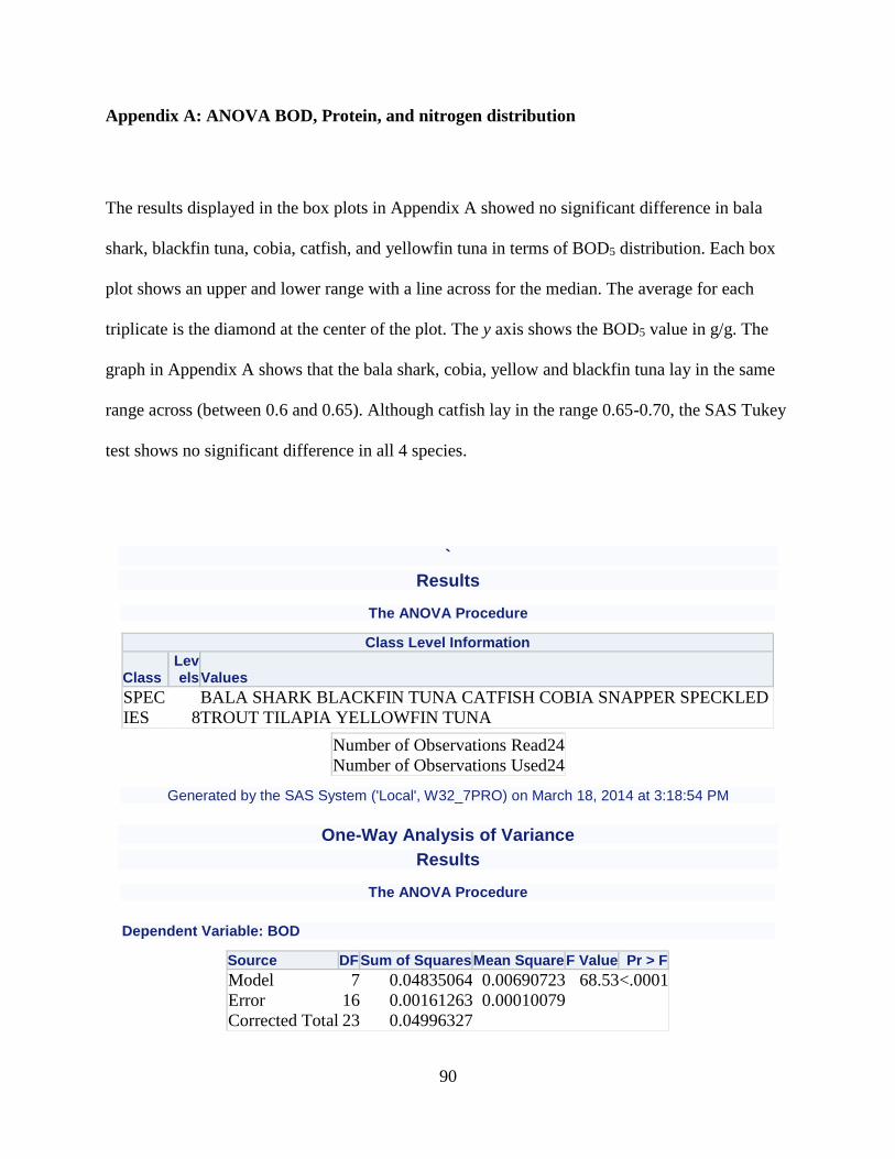
90
Appendix A: ANOVA BOD, Protein, and nitrogen distribution
The results displayed in the box plots in Appendix A showed no significant difference in bala
shark, blackfin tuna, cobia, catfish, and yellowfin tuna in terms of BOD5 distribution. Each box
plot shows an upper and lower range with a line across for the median. The average for each
triplicate is the diamond at the center of the plot. The y axis shows the BOD5 value in g/g. The
graph in Appendix A shows that the bala shark, cobia, yellow and blackfin tuna lay in the same
range across (between 0.6 and 0.65). Although catfish lay in the range 0.65-0.70, the SAS Tukey
test shows no significant difference in all 4 species.
`
Results
The ANOVA Procedure
Class Level Information
Class Levels Values
SPEC
IES 8
BALA SHARK BLACKFIN TUNA CATFISH COBIA SNAPPER SPECKLED
TROUT TILAPIA YELLOWFIN TUNA
Number of Observations Read 24
Number of Observations Used 24
Generated by the SAS System ('Local', W32_7PRO) on March 18, 2014 at 3:18:54 PM
One-Way Analysis of Variance
Results
The ANOVA Procedure
Dependent Variable: BOD
Source DF Sum of Squares Mean Square F Value Pr > F
Model 7 0.04835064 0.00690723 68.53 <.0001
Error 16 0.00161263 0.00010079
Corrected Total 23 0.04996327
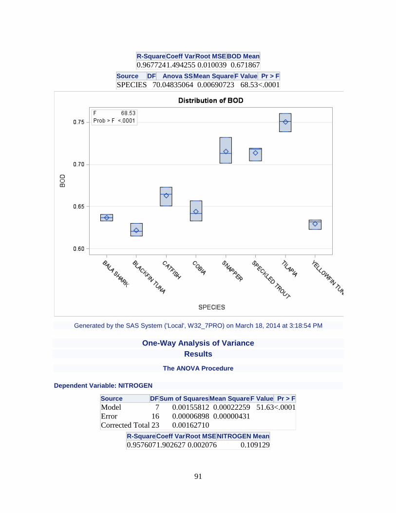
91
R-Square Coeff Var Root MSE BOD Mean
0.967724 1.494255 0.010039 0.671867
Source DF Anova SS Mean Square F Value Pr > F
SPECIES 7 0.04835064 0.00690723 68.53 <.0001
Generated by the SAS System ('Local', W32_7PRO) on March 18, 2014 at 3:18:54 PM
One-Way Analysis of Variance
Results
The ANOVA Procedure
Dependent Variable: NITROGEN
Source DF Sum of Squares Mean Square F Value Pr > F
Model 7 0.00155812 0.00022259 51.63 <.0001
Error 16 0.00006898 0.00000431
Corrected Total 23 0.00162710
R-Square Coeff Var Root MSE NITROGEN Mean
0.957607 1.902627 0.002076 0.109129

92
Source DF Anova SS Mean Square F Value Pr > F
SPECIES 7 0.00155812 0.00022259 51.63 <.0001
Generated by the SAS System ('Local', W32_7PRO) on March 18, 2014 at 3:18:54 PM
One-Way Analysis of Variance
Results
The ANOVA Procedure
Dependent Variable: PROTEIN
Source DF Sum of Squares Mean Square F Value Pr > F
Model 7 332.0218453 47.4316922 195.80 <.0001
Error 16 3.8759720 0.2422483
Corrected Total 23 335.8978173
R-Square Coeff Var Root MSE PROTEIN Mean
0.988461 0.711082 0.492187 69.21667
Source DF Anova SS Mean Square F Value Pr > F
SPECIES 7 332.0218453 47.4316922 195.80 <.0001
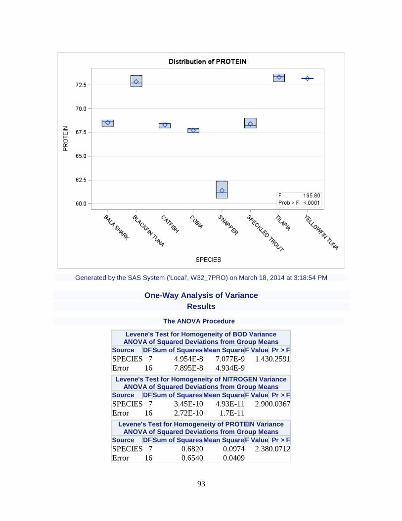
93
Generated by the SAS System ('Local', W32_7PRO) on March 18, 2014 at 3:18:54 PM
One-Way Analysis of Variance
Results
The ANOVA Procedure
Levene's Test for Homogeneity of BOD Variance ANOVA of Squared Deviations from Group Means
Source DF Sum of Squares Mean Square F Value Pr > F
SPECIES 7 4.954E-8 7.077E-9 1.43 0.2591
Error 16 7.895E-8 4.934E-9
Levene's Test for Homogeneity of NITROGEN Variance ANOVA of Squared Deviations from Group Means
Source DF Sum of Squares Mean Square F Value Pr > F
SPECIES 7 3.45E-10 4.93E-11 2.90 0.0367
Error 16 2.72E-10 1.7E-11
Levene's Test for Homogeneity of PROTEIN Variance ANOVA of Squared Deviations from Group Means
Source DF Sum of Squares Mean Square F Value Pr > F
SPECIES 7 0.6820 0.0974 2.38 0.0712
Error 16 0.6540 0.0409
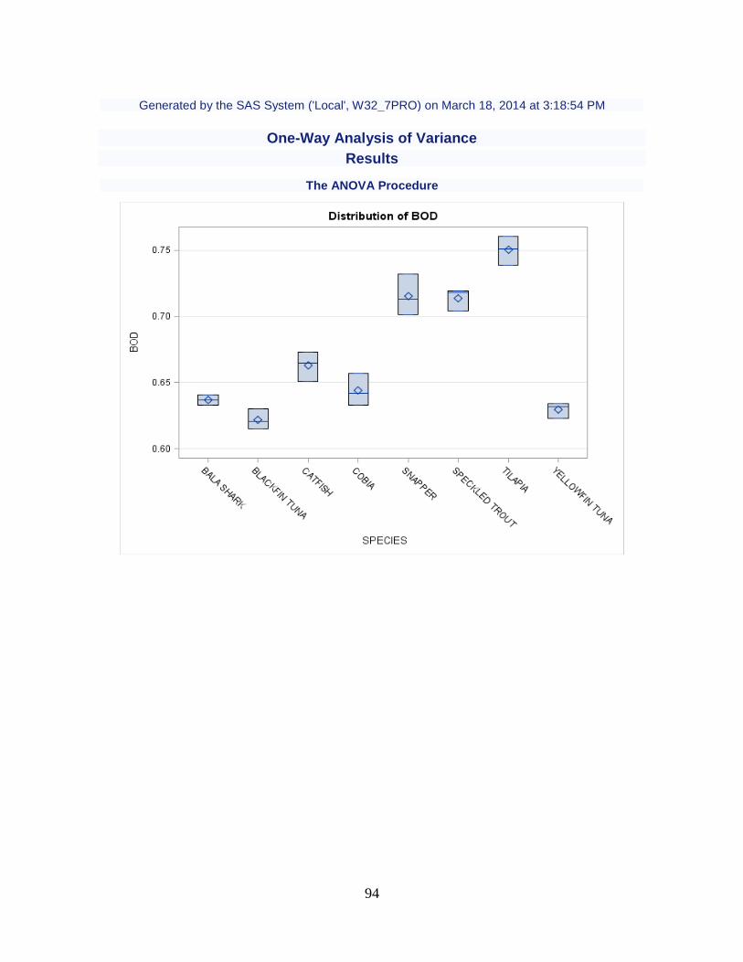
94
Generated by the SAS System ('Local', W32_7PRO) on March 18, 2014 at 3:18:54 PM
One-Way Analysis of Variance
Results
The ANOVA Procedure

95

96
Level of SPECIES N
BOD NITROGEN PROTEIN
Mean Std Dev Mean Std Dev Mean Std Dev
BALA SHARK 3
0.6370000
0
0.0040000
0
0.1098860
0
0.0005785
0
68.549666
7
0.3622959
2
BLACKFIN TUNA 3
0.6220000
0
0.0075498
3
0.1169000
0
0.0011570
1
72.838333
3
0.6009179
1
CATFISH 3
0.6630000
0
0.0111355
3
0.1094250
8
0.0010454
1
68.320000
0
0.2868797
7
COBIA 3
0.6440000
0
0.0121243
6
0.1085500
0
0.0005785
0
67.741666
7
0.2244467
3
SNAPPER 3
0.7154000
0
0.0155396
3
0.0925948
2
0.0018502
8
61.400666
7
0.9162976
2
SPECKLED
TROUT 3
0.7136666
7
0.0083865
0
0.1015126
2
0.0036159
7
68.403333
3
0.5463820
4
TILAPIA 3
0.7502000
0
0.0107782
2
0.1169334
0
0.0038586
8
73.310000
0
0.4160528
8
YELLOWFIN
TUNA 3
0.6296666
7
0.0058594
7
0.1172340
0
0.0000000
0
73.169666
7
0.0414045
1
Generated by the SAS System ('Local', W32_7PRO) on March 18, 2014 at 3:18:54 PM
One-Way Analysis of Variance
Results
The ANOVA Procedure
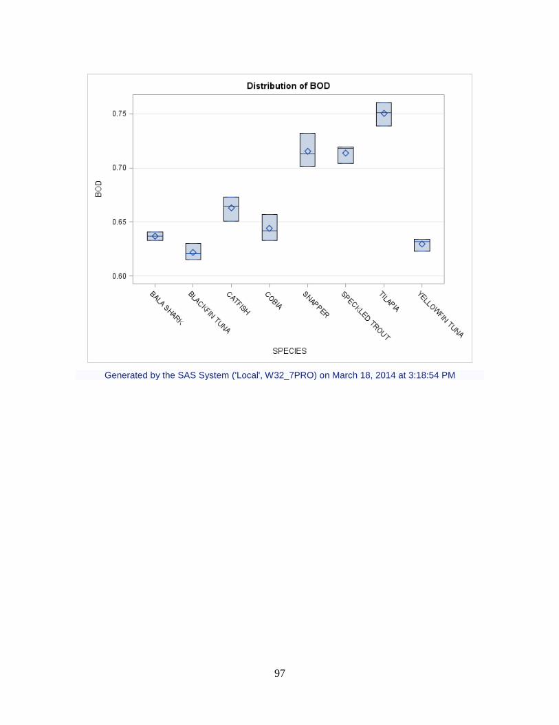
97
Generated by the SAS System ('Local', W32_7PRO) on March 18, 2014 at 3:18:54 PM

98
One-Way Analysis of Variance
Results
The ANOVA Procedure
Tukey's Studentized Range (HSD) Test for BOD
Note: This test controls the Type I experimentwise error rate, but it generally has a higher Type II error rate than REGWQ.
Alpha 0.05
Error Degrees of Freedom 16
Error Mean Square 0.000101
Critical Value of Studentized Range 4.89622
Minimum Significant Difference 0.0284
Means with the same letter are not significantly different.
Tukey Grouping Mean N SPECIES
A 0.750200 3 TILAPIA
B 0.715400 3 SNAPPER
B
B 0.713667 3 SPECKLED TROUT
C 0.663000 3 CATFISH
C
D C 0.644000 3 COBIA
D C
D C 0.637000 3 BALA SHARK
D
D 0.629667 3 YELLOWFIN TUNA
D
D 0.622000 3 BLACKFIN TUNA
Generated by the SAS System ('Local', W32_7PRO) on March 18, 2014 at 3:18:54 PM
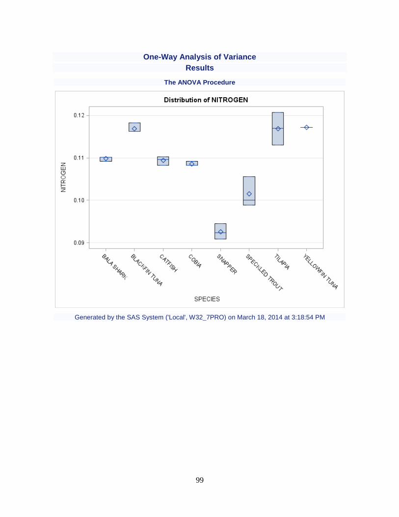
99
One-Way Analysis of Variance
Results
The ANOVA Procedure
Generated by the SAS System ('Local', W32_7PRO) on March 18, 2014 at 3:18:54 PM
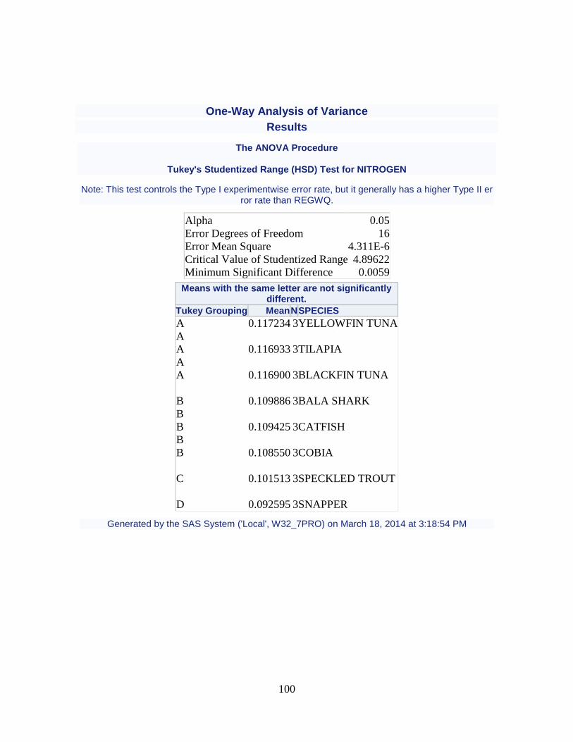
100
One-Way Analysis of Variance
Results
The ANOVA Procedure
Tukey's Studentized Range (HSD) Test for NITROGEN
Note: This test controls the Type I experimentwise error rate, but it generally has a higher Type II error rate than REGWQ.
Alpha 0.05
Error Degrees of Freedom 16
Error Mean Square 4.311E-6
Critical Value of Studentized Range 4.89622
Minimum Significant Difference 0.0059
Means with the same letter are not significantly different.
Tukey Grouping Mean N SPECIES
A 0.117234 3 YELLOWFIN TUNA
A
A 0.116933 3 TILAPIA
A
A 0.116900 3 BLACKFIN TUNA
B 0.109886 3 BALA SHARK
B
B 0.109425 3 CATFISH
B
B 0.108550 3 COBIA
C 0.101513 3 SPECKLED TROUT
D 0.092595 3 SNAPPER
Generated by the SAS System ('Local', W32_7PRO) on March 18, 2014 at 3:18:54 PM

101
One-Way Analysis of Variance
Results
The ANOVA Procedure
Generated by the SAS System ('Local', W32_7PRO) on March 18, 2014 at 3:18:54 PM

102
One-Way Analysis of Variance
Results
The ANOVA Procedure
Tukey's Studentized Range (HSD) Test for PROTEIN
Note: This test controls the Type I experimentwise error rate, but it generally has a higher Type II error rate than REGWQ.
Alpha 0.05
Error Degrees of Freedom 16
Error Mean Square 0.242248
Critical Value of Studentized Range 4.89622
Minimum Significant Difference 1.3913
Means with the same letter are not significantly different.
Tukey Grouping Mean N SPECIES
A 73.3100 3 TILAPIA
A
A 73.1697 3 YELLOWFIN TUNA
A
A 72.8383 3 BLACKFIN TUNA
B 68.5497 3 BALA SHARK
B
B 68.4033 3 SPECKLED TROUT
B
B 68.3200 3 CATFISH
B
B 67.7417 3 COBIA
C 61.4007 3 SNAPPER
Generated by the SAS System ('Local', W32_7PRO) on March 18, 2014 at 3:18:54 PM
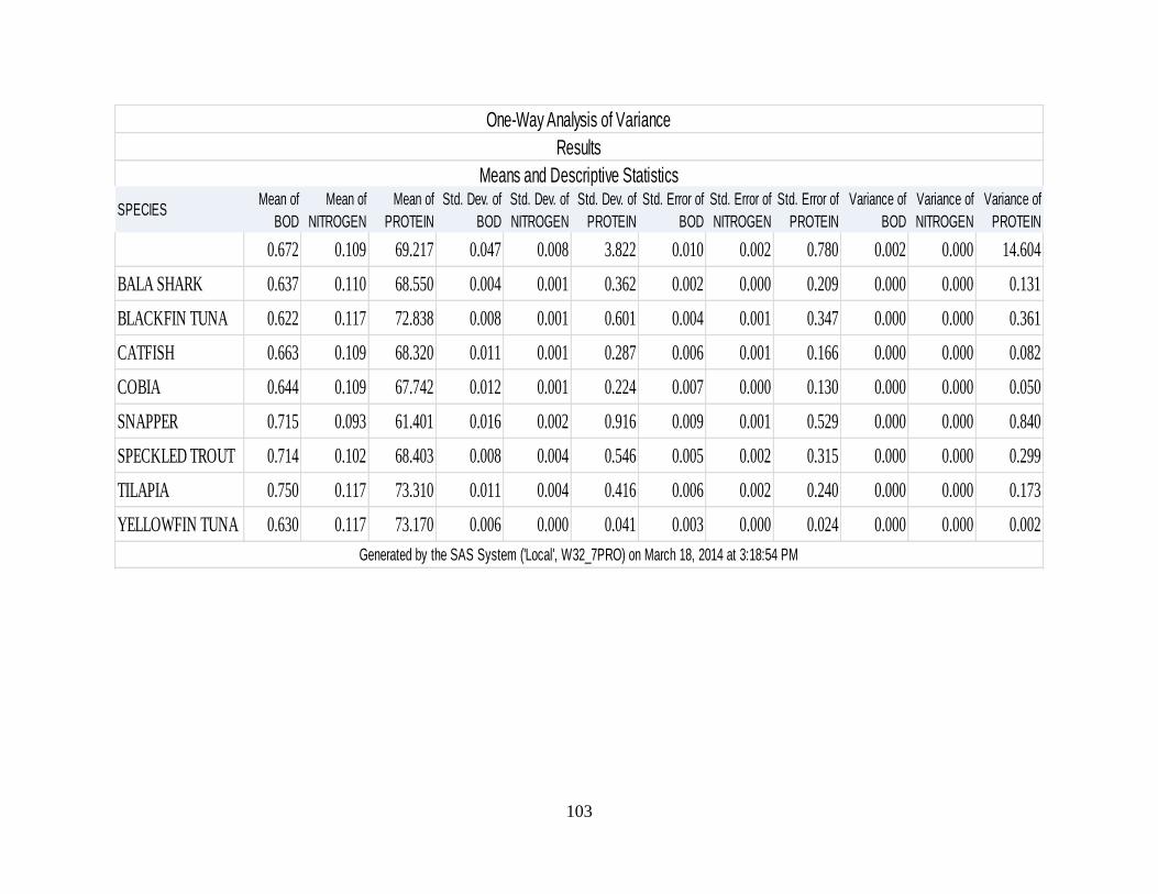
103
SPECIESMean of
BOD
Mean of
NITROGEN
Mean of
PROTEIN
Std. Dev. of
BOD
Std. Dev. of
NITROGEN
Std. Dev. of
PROTEIN
Std. Error of
BOD
Std. Error of
NITROGEN
Std. Error of
PROTEIN
Variance of
BOD
Variance of
NITROGEN
Variance of
PROTEIN
0.672 0.109 69.217 0.047 0.008 3.822 0.010 0.002 0.780 0.002 0.000 14.604
BALA SHARK 0.637 0.110 68.550 0.004 0.001 0.362 0.002 0.000 0.209 0.000 0.000 0.131
BLACKFIN TUNA 0.622 0.117 72.838 0.008 0.001 0.601 0.004 0.001 0.347 0.000 0.000 0.361
CATFISH 0.663 0.109 68.320 0.011 0.001 0.287 0.006 0.001 0.166 0.000 0.000 0.082
COBIA 0.644 0.109 67.742 0.012 0.001 0.224 0.007 0.000 0.130 0.000 0.000 0.050
SNAPPER 0.715 0.093 61.401 0.016 0.002 0.916 0.009 0.001 0.529 0.000 0.000 0.840
SPECKLED TROUT 0.714 0.102 68.403 0.008 0.004 0.546 0.005 0.002 0.315 0.000 0.000 0.299
TILAPIA 0.750 0.117 73.310 0.011 0.004 0.416 0.006 0.002 0.240 0.000 0.000 0.173
YELLOWFIN TUNA 0.630 0.117 73.170 0.006 0.000 0.041 0.003 0.000 0.024 0.000 0.000 0.002
Generated by the SAS System ('Local', W32_7PRO) on March 18, 2014 at 3:18:54 PM
One-Way Analysis of Variance
Results
Means and Descriptive Statistics
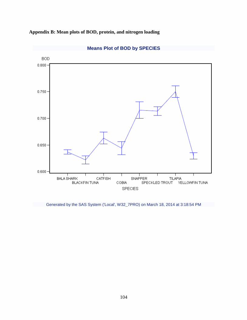
104
Appendix B: Mean plots of BOD, protein, and nitrogen loading
Means Plot of BOD by SPECIES
Generated by the SAS System ('Local', W32_7PRO) on March 18, 2014 at 3:18:54 PM

105
Means Plot of NITROGEN by SPECIES
Generated by the SAS System ('Local', W32_7PRO) on March 18, 2014 at 3:18:54 PM
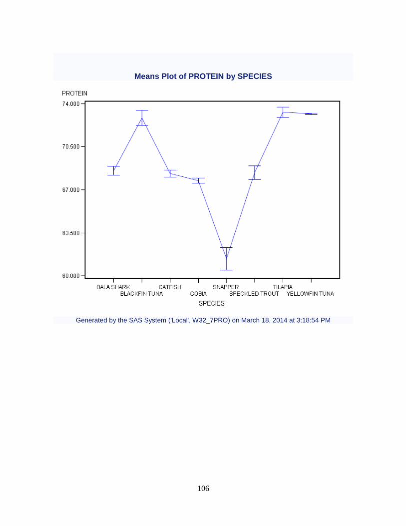
106
Means Plot of PROTEIN by SPECIES
Generated by the SAS System ('Local', W32_7PRO) on March 18, 2014 at 3:18:54 PM

107
Appendix C: Fingerling and Growout Assumptions
C.1. Fingerling Assumptions
The fingerling tank volume allows us to calculate the maximum feed (𝐹𝑡𝑚𝑎𝑥𝑓
) allowed. 𝐹𝑡𝑚𝑎𝑥𝑓
,
equals the tank volume (𝑉𝑡𝑓) divided by the recirculation rate (𝑣𝑟
𝑓), which is, 400 gal/lb. feed. The
bead volume (𝑉𝑏𝑓) is calculated by dividing 𝐹𝑡𝑚𝑎𝑥
𝑓 by the bead volume rate (𝑣𝑏
𝑓), that is, 0.75
ft³/lb./day. The bead filter size for each tank (𝐹𝑠𝑓) is 𝑉𝑏
𝑓 divided by𝑁𝑓
𝑓, the number of bead filters
per tank. The maximum production cost per tank per year (𝑃𝑚𝑎𝑥𝑓
) is 𝐹𝑡𝑚𝑎𝑥𝑓
divided the feed ratio
F/C multiplied by annual cycle 𝐴𝑐, 350 days for the annual cycle length. The maximum holding
capacity 𝐻𝑐𝑚𝑎𝑥𝑓
is 𝐹𝑡𝑚𝑎𝑥𝑓
divided by the feed rate 𝑓𝑏𝑚𝑓
that is, 5 percent of body mass divided by the
mortality rate 𝑀𝑟𝑓 at 0.95. The density (𝛿𝑓) is given by 𝐻𝑐𝑚𝑎𝑥
𝑓 divided by𝑉𝑡
𝑓. The circulation (𝐶𝑡
𝑓)
is 𝐹𝑡𝑚𝑎𝑥𝑓
divided by the circulation rate 𝑞𝑟𝑓 which is 10 gpm/lb. feed/day. Chemicals (mainly
bicarbonate) help ensure appropriate alkalinity levels in the tank water. The amount of bi-carb
NaHCO₃ per tank is obtained by multiplying 𝐹𝑡𝑚𝑎𝑥𝑓
by the bi-carb daily dosage 𝑏𝑎𝑓 and by 𝐴𝑐 at
0.24 lb. bi-carb/lbs. feed. This means that chemical dosing is determined based on the amount of
feeding administered, with a chemical/feeding ratio of 0.24 in lbs. The air needed for the airstone
or aeration (𝐴𝑠𝑓) is given by the airstone rate (𝑔𝑎
𝑓) at 4 scfh/lbs. feed-day multiplied by 𝐹𝑡𝑚𝑎𝑥
𝑓. The
flushing rate 𝑄𝑓𝑓 equals 𝐹𝑡𝑚𝑎𝑥
𝑓 multiplied by the water replacement rate 𝑞𝑓 at 24.7 gal/lbs. feed/day.
The tank recirculation rate 𝑄𝑟𝑓 is the circulation rate 𝑞𝑟
𝑓 multiplied by𝐹𝑡𝑚𝑎𝑥
𝑓. The number of
fingerling 𝑁𝑓 equal to the 𝐻𝑐𝑚𝑎𝑥𝑓
multiplied by holding cycle 2.89 and the mortality rate 𝑀𝑟𝑓
divided by average fingerling size 𝑓𝑠𝑓 at 25 g or 0.06 lbs. The weight at harvest 𝑊𝑡 is equal to
number of fingerling 𝑁𝑓 multiplied by harvest size of fingerling ℎ𝑠 at 50 g or 0.12 lbs. The feed
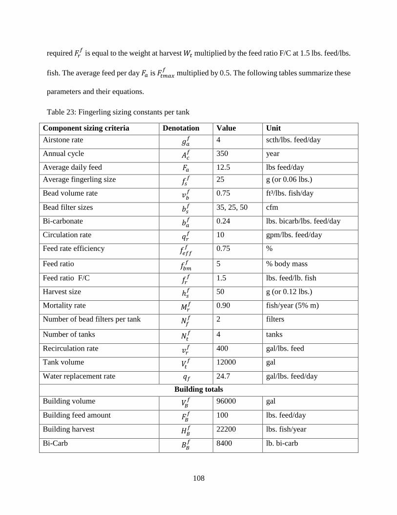
108
required 𝐹𝑟𝑓 is equal to the weight at harvest 𝑊𝑡 multiplied by the feed ratio F/C at 1.5 lbs. feed/lbs.
fish. The average feed per day 𝐹𝑎 is 𝐹𝑡𝑚𝑎𝑥𝑓
multiplied by 0.5. The following tables summarize these
parameters and their equations.
Table 23: Fingerling sizing constants per tank
Component sizing criteria Denotation Value Unit
Airstone rate 𝑔𝑎𝑓 4 scth/lbs. feed/day
Annual cycle 𝐴𝑐𝑓 350 year
Average daily feed 𝐹𝑎 12.5 lbs feed/day
Average fingerling size 𝑓𝑠𝑓 25 g (or 0.06 lbs.)
Bead volume rate 𝑣𝑏𝑓 0.75 ft³/lbs. fish/day
Bead filter sizes 𝑏𝑠𝑓 35, 25, 50 cfm
Bi-carbonate 𝑏𝑎𝑓 0.24 lbs. bicarb/lbs. feed/day
Circulation rate 𝑞𝑟𝑓 10 gpm/lbs. feed/day
Feed rate efficiency 𝑓𝑒𝑓𝑓𝑓
0.75 %
Feed ratio 𝑓𝑏𝑚𝑓
5 % body mass
Feed ratio F/C 𝑓𝑟𝑓 1.5 lbs. feed/lb. fish
Harvest size ℎ𝑠𝑓 50 g (or 0.12 lbs.)
Mortality rate 𝑀𝑟𝑓 0.90 fish/year (5% m)
Number of bead filters per tank 𝑁𝑓𝑓 2 filters
Number of tanks 𝑁𝑡𝑓 4 tanks
Recirculation rate 𝑣𝑟𝑓 400 gal/lbs. feed
Tank volume 𝑉𝑡𝑓 12000 gal
Water replacement rate 𝑞𝑓 24.7 gal/lbs. feed/day
Building totals
Building volume 𝑉𝐵𝑓 96000 gal
Building feed amount 𝐹𝐵𝑓 100 lbs. feed/day
Building harvest 𝐻𝐵𝑓 22200 lbs. fish/year
Bi-Carb 𝐵𝐵𝑓 8400 lb. bi-carb
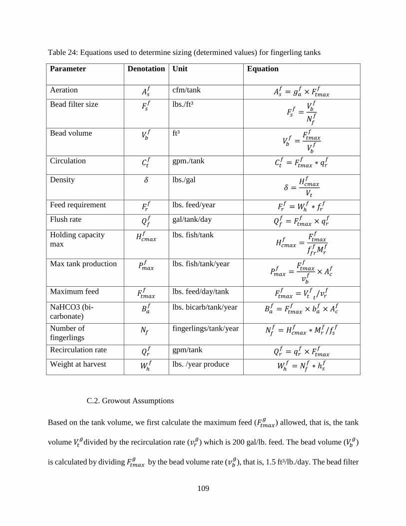
109
Table 24: Equations used to determine sizing (determined values) for fingerling tanks
Parameter Denotation Unit Equation
Aeration 𝐴𝑠𝑓 cfm/tank 𝐴𝑠
𝑓= 𝑔𝑎
𝑓× 𝐹𝑡𝑚𝑎𝑥
𝑓
Bead filter size 𝐹𝑠𝑓 lbs./ft³
𝐹𝑠𝑓
=𝑉𝑏
𝑓
𝑁𝑓𝑓
Bead volume 𝑉𝑏𝑓 ft³
𝑉𝑏𝑓
=𝐹𝑡𝑚𝑎𝑥
𝑓
𝑉𝑏𝑓
Circulation 𝐶𝑡𝑓 gpm./tank 𝐶𝑡
𝑓= 𝐹𝑡𝑚𝑎𝑥
𝑓∗ 𝑞𝑟
𝑓
Density 𝛿 lbs./gal
𝛿 =
𝐻𝑐𝑚𝑎𝑥𝑓
𝑉𝑡
Feed requirement 𝐹𝑟𝑓 lbs. feed/year 𝐹𝑟
𝑓= 𝑊ℎ
𝑓∗ 𝑓𝑟
𝑓
Flush rate 𝑄𝑓𝑓 gal/tank/day 𝑄𝑓
𝑓= 𝐹𝑡𝑚𝑎𝑥
𝑓× 𝑞𝑟
𝑓
Holding capacity
max 𝐻𝑐𝑚𝑎𝑥
𝑓 lbs. fish/tank
𝐻𝑐𝑚𝑎𝑥
𝑓=
𝐹𝑡𝑚𝑎𝑥𝑓
𝑓𝑓𝑟𝑓
𝑀𝑟𝑓
Max tank production 𝑃𝑚𝑎𝑥𝑓
lbs. fish/tank/year 𝑃𝑚𝑎𝑥
𝑓=
𝐹𝑡𝑚𝑎𝑥𝑓
𝑣𝑏𝑓
× 𝐴𝑐𝑓
Maximum feed 𝐹𝑡𝑚𝑎𝑥𝑓
lbs. feed/day/tank 𝐹𝑡𝑚𝑎𝑥𝑓
= 𝑉𝑡𝑓
𝑡/𝑣𝑟
𝑓
NaHCO3 (bi-
carbonate) 𝐵𝑎
𝑓 lbs. bicarb/tank/year 𝐵𝑎
𝑓= 𝐹𝑡𝑚𝑎𝑥
𝑓× 𝑏𝑎
𝑓× 𝐴𝑐
𝑓
Number of
fingerlings 𝑁𝑓 fingerlings/tank/year 𝑁𝑓
𝑓= 𝐻𝑐𝑚𝑎𝑥
𝑓∗ 𝑀𝑟
𝑓/𝑓𝑠
𝑓
Recirculation rate 𝑄𝑟𝑓 gpm/tank 𝑄𝑟
𝑓= 𝑞𝑟
𝑓× 𝐹𝑡𝑚𝑎𝑥
𝑓
Weight at harvest 𝑊ℎ𝑓 lbs. /year produce 𝑊ℎ
𝑓= 𝑁𝑓
𝑓∗ ℎ𝑠
𝑓
C.2. Growout Assumptions
Based on the tank volume, we first calculate the maximum feed (𝐹𝑡𝑚𝑎𝑥𝑔
) allowed, that is, the tank
volume 𝑉𝑡𝑔
divided by the recirculation rate (𝑣𝑟𝑔
) which is 200 gal/lb. feed. The bead volume (𝑉𝑏𝑔
)
is calculated by dividing 𝐹𝑡𝑚𝑎𝑥 𝑔
by the bead volume rate (𝑣𝑏𝑔
), that is, 1.5 ft³/lb./day. The bead filter
110
size for each tank (𝐹𝑠𝑔
) is 𝑉𝑏 divided by the number of bead filters per tank. The maximum
production cost per tank per year (𝑃𝑚𝑎𝑥𝑔
) is
𝐹𝑡𝑚𝑎𝑥 𝑔
divided by 𝑣𝑏𝑔
multiplied by 350 days, that is, the annual cycle length otherwise referred to
as𝐴𝑐𝑔
. The maximum holding capacity 𝐻𝑐𝑚𝑎𝑥𝑔
is 𝐹𝑡𝑚𝑎𝑥 𝑔
divided by the feed ratio or feed rate (𝑓𝑟𝑔
),
that is, 0.015 lb. feed/lb. fish/day. The density (𝛿𝑔) is given by 𝐻𝑐𝑚𝑎𝑥𝑔
divided by𝑉𝑡𝑔
. The
circulation (𝐶𝑡𝑔
) is 𝐹𝑡𝑚𝑎𝑥 𝑔
divided by the circulation rate 𝑞𝑟. The amount of bi-carb NaHCO₃ per
tank is obtained by multiplying 𝐹𝑡𝑚𝑎𝑥𝑔
by the bi-carb daily dosage 𝑏𝑎𝑔
and by𝐴𝑐𝑔
. The air needed for
the airstone (𝐴𝑠𝑔
) is given by the airstone rate (𝑔𝑎𝑔
) multiplied by 𝐹𝑡𝑚𝑎𝑥𝑔
. The flush rate per day
𝑄𝑓𝑔
equals 𝐹𝑡𝑚𝑎𝑥 𝑔
multiplied by the water replacement rate 𝑞𝑟𝑔
. The circulation rate 𝑄𝑟𝑔
is 𝑞𝑟𝑔
multiplied by 𝐹𝑡𝑚𝑎𝑥𝑔
. To calculate the number of growout 𝑁𝑔, we divide 𝑃𝑚𝑎𝑥𝑔
by the product of
the harvest weight (𝐻𝑤) – the average weight of one fish at harvest time – and the feed rate
efficiency (𝑓𝑒𝑓𝑓𝑔
).
The following tables summarize these parameters and their equations.
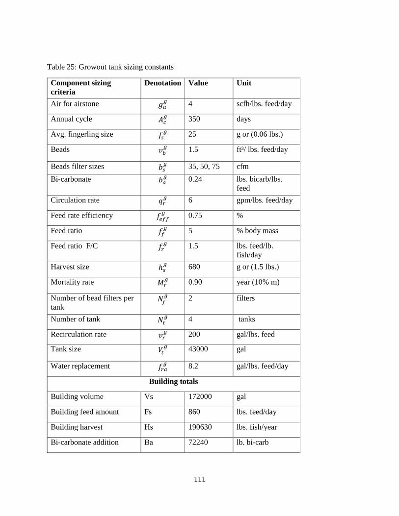
111
Table 25: Growout tank sizing constants
Component sizing
criteria
Denotation Value Unit
Air for airstone 𝑔𝑎𝑔
4 scfh/lbs. feed/day
Annual cycle 𝐴𝑐𝑔
350 days
Avg. fingerling size 𝑓𝑠𝑔
25 g or (0.06 lbs.)
Beads 𝑣𝑏𝑔
1.5 ft³/ lbs. feed/day
Beads filter sizes 𝑏𝑠𝑔
35, 50, 75 cfm
Bi-carbonate 𝑏𝑎𝑔
0.24 lbs. bicarb/lbs.
feed
Circulation rate 𝑞𝑟𝑔
6 gpm/lbs. feed/day
Feed rate efficiency 𝑓𝑒𝑓𝑓𝑔
0.75 %
Feed ratio 𝑓𝑓𝑔
5 % body mass
Feed ratio F/C 𝑓𝑟𝑔
1.5 lbs. feed/lb.
fish/day
Harvest size ℎ𝑠𝑔
680 g or (1.5 lbs.)
Mortality rate 𝑀𝑟𝑔
0.90 year (10% m)
Number of bead filters per
tank 𝑁𝑓
𝑔 2 filters
Number of tank 𝑁𝑡𝑔
4 tanks
Recirculation rate 𝑣𝑟𝑔
200 gal/lbs. feed
Tank size 𝑉𝑡𝑔
43000 gal
Water replacement 𝑓𝑟𝑎𝑔
8.2 gal/lbs. feed/day
Building totals
Building volume Vs 172000 gal
Building feed amount Fs 860 lbs. feed/day
Building harvest Hs 190630 lbs. fish/year
Bi-carbonate addition Ba 72240 lb. bi-carb
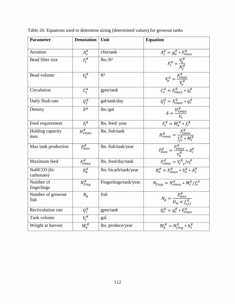
112
Table 26: Equations used to determine sizing (determined values) for growout tanks
Parameter Denotation Unit Equation
Aeration 𝐴𝑠𝑔
cfm/tank 𝐴𝑠𝑔
= 𝑔𝑎𝑔
∗ 𝐹𝑡𝑚𝑎𝑥𝑔
Bead filter size 𝐹𝑠𝑔
lbs./ft³ 𝐹𝑠
𝑔=
𝑉𝑏𝑔
𝑁𝑓𝑔
Bead volume 𝑉𝑏𝑔
ft³ 𝑉𝑏
𝑔=
𝐹𝑡𝑚𝑎𝑥𝑔
𝑉𝑏𝑔
Circulation 𝐶𝑡𝑔
gpm/tank 𝐶𝑡𝑔
= 𝐹𝑡𝑚𝑎𝑥𝑔
∗ 𝑞𝑟𝑔
Daily flush rate 𝑄𝑓𝑔
gal/tank/day 𝑄𝑓𝑔
= 𝐹𝑡𝑚𝑎𝑥𝑔
∗ 𝑞𝑟𝑔
Density 𝛿𝑔 lbs./gal
𝛿 =
𝐻𝑐𝑚𝑎𝑥𝑔
𝑉𝑡
Feed requirement 𝐹𝑟𝑔
lbs. feed/ year 𝐹𝑟𝑔
= 𝑊ℎ𝑔
∗ 𝑓𝑟𝑔
Holding capacity
max 𝐻𝑐𝑚𝑎𝑥
𝑔 lbs. fish/tank
𝐻𝑐𝑚𝑎𝑥
𝑔=
𝐹𝑡𝑚𝑎𝑥𝑔
𝑓𝑓𝑟𝑔
∗ 𝑀𝑟𝑔
Max tank production 𝑃𝑚𝑎𝑥𝑔
lbs. fish/tank/year 𝑃𝑚𝑎𝑥
𝑔=
𝐹𝑡𝑚𝑎𝑥𝑔
𝑣𝑏𝑔 ∗ 𝐴𝑐
𝑔
Maximum feed 𝐹𝑡𝑚𝑎𝑥𝑔
lbs. feed/day/tank 𝐹𝑡𝑚𝑎𝑥𝑔
= 𝑉𝑡𝑔
𝑡/𝑣𝑟
𝑔
NaHCO3 (bi-
carbonate) 𝐵𝑎
𝑔 lbs. bicarb/tank/year 𝐵𝑎
𝑔= 𝐹𝑡𝑚𝑎𝑥
𝑔∗ 𝑏𝑎
𝑔∗ 𝐴𝑐
𝑔
Number of
fingerlings 𝑁𝑓𝑖𝑛𝑔
𝑔 Fingerlings/tank/year. 𝑁𝑓𝑖𝑛𝑔 = 𝐻𝑐𝑚𝑎𝑥
𝑔∗ 𝑀𝑟
𝑔/𝑓𝑠
𝑔
Number of growout
fish 𝑁𝑔 fish
𝑁𝑔 =𝑃𝑚𝑎𝑥
𝑔
𝐻𝑤 × 𝑓𝑒𝑓𝑓𝑔
Recirculation rate 𝑄𝑟𝑔
gpm/tank 𝑄𝑟𝑔
= 𝑞𝑟𝑔
∗ 𝐹𝑡𝑚𝑎𝑥𝑔
Tank volume 𝑉𝑡𝑔
gal.
Weight at harvest 𝑊ℎ𝑔
lbs. produce/year 𝑊ℎ𝑔
= 𝑁𝑓𝑖𝑛𝑔𝑔
∗ ℎ𝑠𝑔
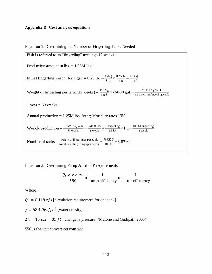
113
Appendix D: Cost analysis equations
Equation 1: Determining the Number of Fingerling Tanks Needed
Fish is referred to as “fingerling” until age 12 weeks.
Production amount in lbs. = 1.25M lbs.
Initial fingerling weight for 1 gal. = 0.25 lb. =454 g
1 lb.×
0.25 lb.
1 g=
113.5g
1 gal.
Weight of fingerling per tank (12 weeks) = 113.5 g
1 gal.×75000 gal.=
70937.5 g/tank
12 weeks in fingerling tank
1 year = 50 weeks
Annual production = 1.25M lbs. /year; Mortality rates 10%
Weekly production = 1.25M lbs./year
50 weeks=
25000 lbs.
1 week×
1 fingerling
1.5 lb.×1.1=
18333 fingerling
1 week
Number of tanks = weight of fingerlings per tank
number of fingerlings per week=
70937.5
18333=3.87≃4
Equation 2: Determining Pump Airlift HP requirements
𝑄𝑟 × 𝛾 × ∆ℎ
550×
1
pump efficiency×
1
motor efficiency
Where
𝑄𝑟 = 0.448 𝑐𝑓𝑠 [circulation requirement for one tank]
𝛾 = 62.4 𝑙𝑏𝑠./𝑓𝑡.2 [water density]
∆ℎ = 15 𝑝𝑠𝑖 = 35 𝑓𝑡. [change is pressure] (Malone and Gudipati, 2005)
550 is the unit conversion constant
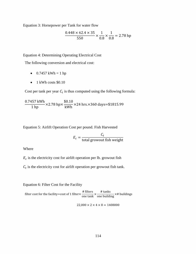
114
Equation 3: Horsepower per Tank for water flow
0.448 × 62.4 × 35
550×
1
0.8×
1
0.8= 2.78 hp
Equation 4: Determining Operating Electrical Cost
The following conversion and electrical cost:
0.7457 kWh = 1 hp
1 kWh costs $0.10
Cost per tank per year 𝐶𝑡 is thus computed using the following formula:
0.7457 kWh
1 hp×2.78 hp×
$0.10
kWh×24 hrs.×360 days=$1815.99
Equation 5: Airlift Operation Cost per pound. Fish Harvested
𝐸𝑐 =𝐶𝑡
total growout fish weight
Where
𝐸𝑐 is the electricity cost for airlift operation per lb. growout fish
𝐶𝑡 is the electricity cost for airlift operation per growout fish tank.
Equation 6: Filter Cost for the Facility
filter cost for the facility=cost of 1 filter×# filters
one tank×
# tanks
one building×# buildings
22,000 × 2 × 4 × 8 = 1408000
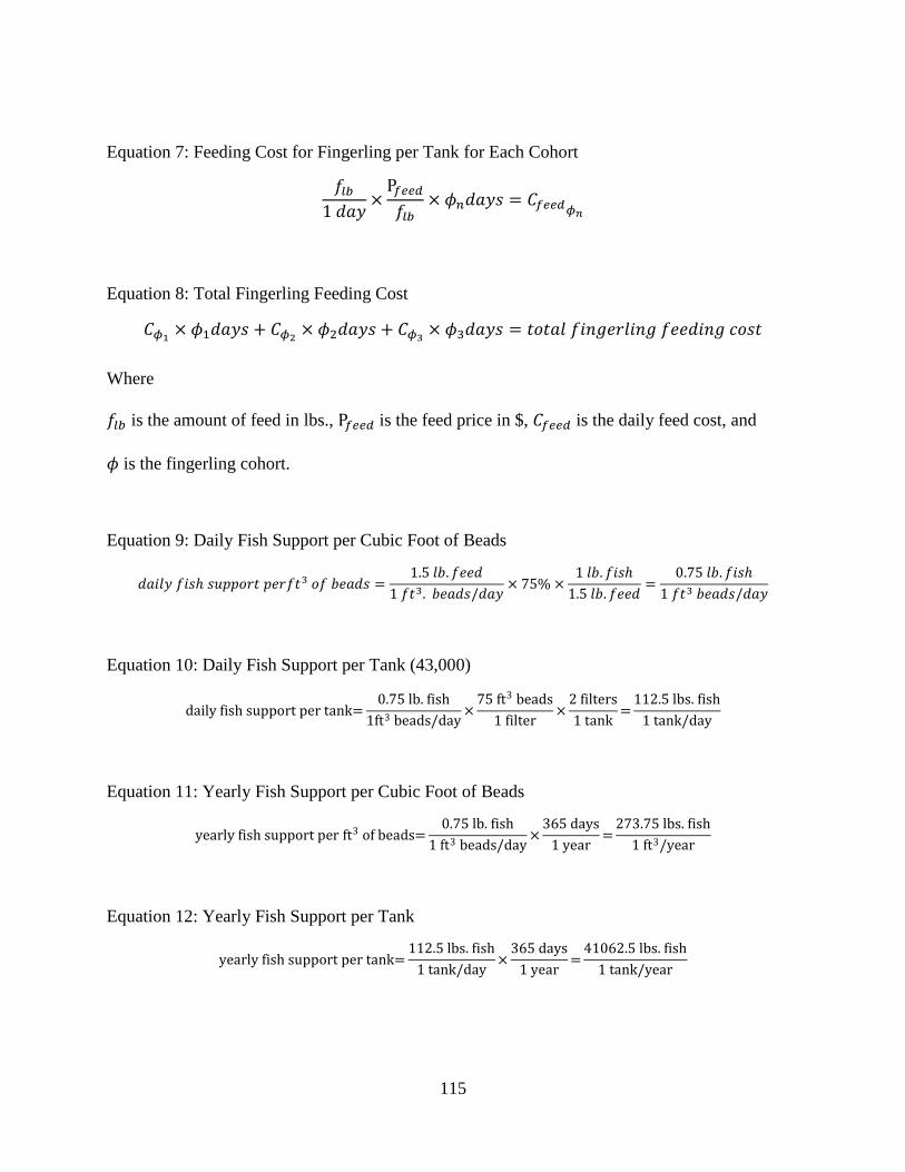
115
Equation 7: Feeding Cost for Fingerling per Tank for Each Cohort
𝑓𝑙𝑏
1 𝑑𝑎𝑦×
Ρ𝑓𝑒𝑒𝑑
𝑓𝑙𝑏× 𝜙𝑛𝑑𝑎𝑦𝑠 = 𝐶𝑓𝑒𝑒𝑑𝜙𝑛
Equation 8: Total Fingerling Feeding Cost
𝐶𝜙1× 𝜙1𝑑𝑎𝑦𝑠 + 𝐶𝜙2
× 𝜙2𝑑𝑎𝑦𝑠 + 𝐶𝜙3× 𝜙3𝑑𝑎𝑦𝑠 = 𝑡𝑜𝑡𝑎𝑙 𝑓𝑖𝑛𝑔𝑒𝑟𝑙𝑖𝑛𝑔 𝑓𝑒𝑒𝑑𝑖𝑛𝑔 𝑐𝑜𝑠𝑡
Where
𝑓𝑙𝑏 is the amount of feed in lbs., Ρ𝑓𝑒𝑒𝑑 is the feed price in $, 𝐶𝑓𝑒𝑒𝑑 is the daily feed cost, and
𝜙 is the fingerling cohort.
Equation 9: Daily Fish Support per Cubic Foot of Beads
𝑑𝑎𝑖𝑙𝑦 𝑓𝑖𝑠ℎ 𝑠𝑢𝑝𝑝𝑜𝑟𝑡 𝑝𝑒𝑟𝑓𝑡3 𝑜𝑓 𝑏𝑒𝑎𝑑𝑠 =1.5 𝑙𝑏. 𝑓𝑒𝑒𝑑
1 𝑓𝑡3. 𝑏𝑒𝑎𝑑𝑠/𝑑𝑎𝑦× 75% ×
1 𝑙𝑏. 𝑓𝑖𝑠ℎ
1.5 𝑙𝑏. 𝑓𝑒𝑒𝑑=
0.75 𝑙𝑏. 𝑓𝑖𝑠ℎ
1 𝑓𝑡3 𝑏𝑒𝑎𝑑𝑠/𝑑𝑎𝑦
Equation 10: Daily Fish Support per Tank (43,000)
daily fish support per tank=0.75 lb. fish
1ft3 beads/day×
75 ft3 beads
1 filter×
2 filters
1 tank=
112.5 lbs. fish
1 tank/day
Equation 11: Yearly Fish Support per Cubic Foot of Beads
yearly fish support per ft3 of beads=0.75 lb. fish
1 ft3 beads/day×
365 days
1 year=
273.75 lbs. fish
1 ft3/year
Equation 12: Yearly Fish Support per Tank
yearly fish support per tank=112.5 lbs. fish
1 tank/day×
365 days
1 year=
41062.5 lbs. fish
1 tank/year
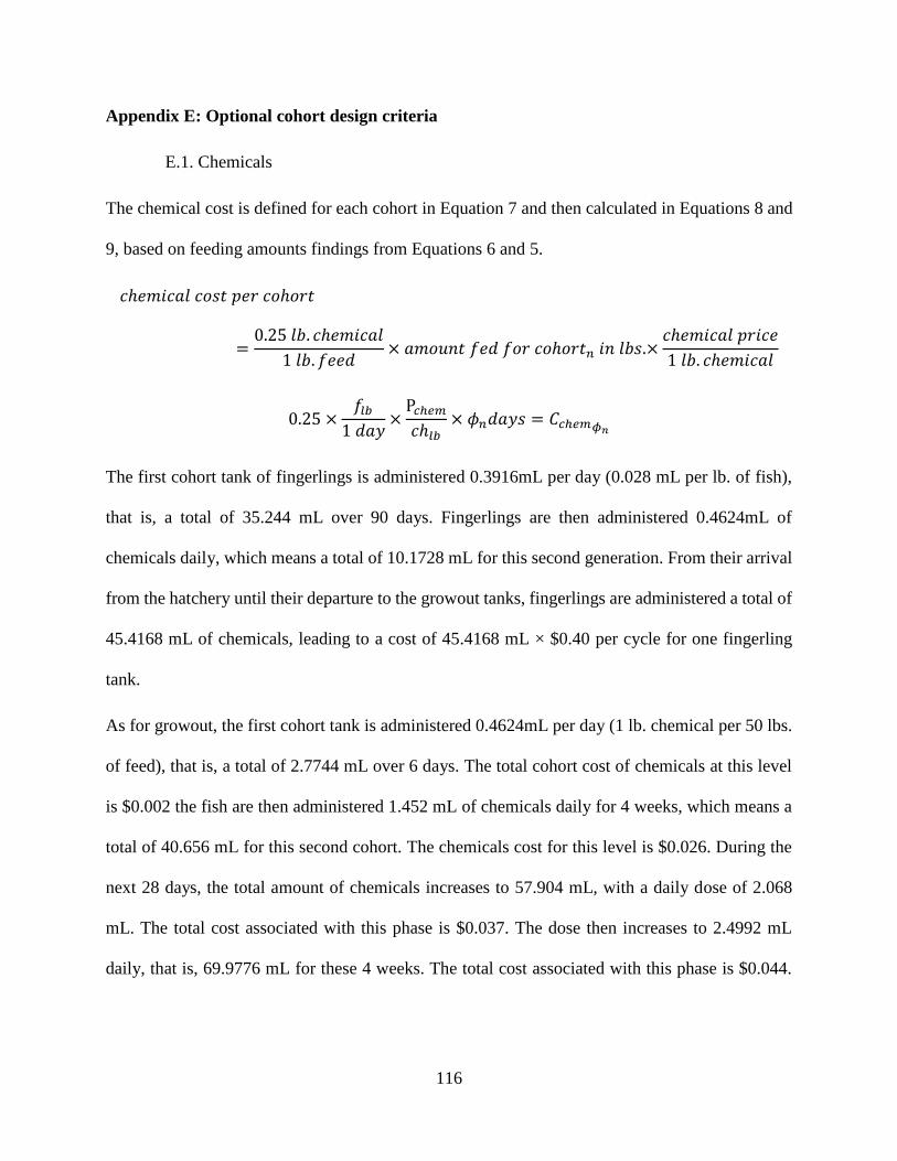
116
Appendix E: Optional cohort design criteria
E.1. Chemicals
The chemical cost is defined for each cohort in Equation 7 and then calculated in Equations 8 and
9, based on feeding amounts findings from Equations 6 and 5.
𝑐ℎ𝑒𝑚𝑖𝑐𝑎𝑙 𝑐𝑜𝑠𝑡 𝑝𝑒𝑟 𝑐𝑜ℎ𝑜𝑟𝑡
=0.25 𝑙𝑏. 𝑐ℎ𝑒𝑚𝑖𝑐𝑎𝑙
1 𝑙𝑏. 𝑓𝑒𝑒𝑑× 𝑎𝑚𝑜𝑢𝑛𝑡 𝑓𝑒𝑑 𝑓𝑜𝑟 𝑐𝑜ℎ𝑜𝑟𝑡𝑛 𝑖𝑛 𝑙𝑏𝑠.×
𝑐ℎ𝑒𝑚𝑖𝑐𝑎𝑙 𝑝𝑟𝑖𝑐𝑒
1 𝑙𝑏. 𝑐ℎ𝑒𝑚𝑖𝑐𝑎𝑙
0.25 ×𝑓𝑙𝑏
1 𝑑𝑎𝑦×
Ρ𝑐ℎ𝑒𝑚
𝑐ℎ𝑙𝑏× 𝜙𝑛𝑑𝑎𝑦𝑠 = 𝐶𝑐ℎ𝑒𝑚𝜙𝑛
The first cohort tank of fingerlings is administered 0.3916mL per day (0.028 mL per lb. of fish),
that is, a total of 35.244 mL over 90 days. Fingerlings are then administered 0.4624mL of
chemicals daily, which means a total of 10.1728 mL for this second generation. From their arrival
from the hatchery until their departure to the growout tanks, fingerlings are administered a total of
45.4168 mL of chemicals, leading to a cost of 45.4168 mL × $0.40 per cycle for one fingerling
tank.
As for growout, the first cohort tank is administered 0.4624mL per day (1 lb. chemical per 50 lbs.
of feed), that is, a total of 2.7744 mL over 6 days. The total cohort cost of chemicals at this level
is $0.002 the fish are then administered 1.452 mL of chemicals daily for 4 weeks, which means a
total of 40.656 mL for this second cohort. The chemicals cost for this level is $0.026. During the
next 28 days, the total amount of chemicals increases to 57.904 mL, with a daily dose of 2.068
mL. The total cost associated with this phase is $0.037. The dose then increases to 2.4992 mL
daily, that is, 69.9776 mL for these 4 weeks. The total cost associated with this phase is $0.044.
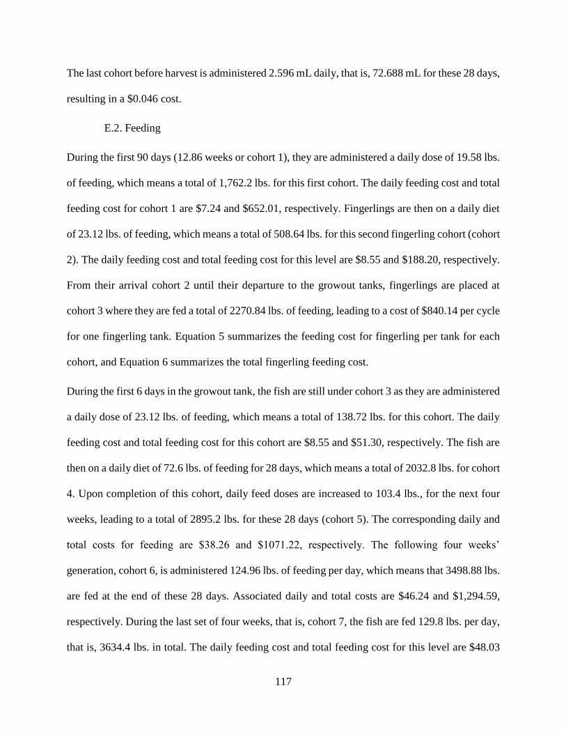
117
The last cohort before harvest is administered 2.596 mL daily, that is, 72.688 mL for these 28 days,
resulting in a $0.046 cost.
E.2. Feeding
During the first 90 days (12.86 weeks or cohort 1), they are administered a daily dose of 19.58 lbs.
of feeding, which means a total of 1,762.2 lbs. for this first cohort. The daily feeding cost and total
feeding cost for cohort 1 are $7.24 and $652.01, respectively. Fingerlings are then on a daily diet
of 23.12 lbs. of feeding, which means a total of 508.64 lbs. for this second fingerling cohort (cohort
2). The daily feeding cost and total feeding cost for this level are $8.55 and $188.20, respectively.
From their arrival cohort 2 until their departure to the growout tanks, fingerlings are placed at
cohort 3 where they are fed a total of 2270.84 lbs. of feeding, leading to a cost of $840.14 per cycle
for one fingerling tank. Equation 5 summarizes the feeding cost for fingerling per tank for each
cohort, and Equation 6 summarizes the total fingerling feeding cost.
During the first 6 days in the growout tank, the fish are still under cohort 3 as they are administered
a daily dose of 23.12 lbs. of feeding, which means a total of 138.72 lbs. for this cohort. The daily
feeding cost and total feeding cost for this cohort are $8.55 and $51.30, respectively. The fish are
then on a daily diet of 72.6 lbs. of feeding for 28 days, which means a total of 2032.8 lbs. for cohort
4. Upon completion of this cohort, daily feed doses are increased to 103.4 lbs., for the next four
weeks, leading to a total of 2895.2 lbs. for these 28 days (cohort 5). The corresponding daily and
total costs for feeding are $38.26 and $1071.22, respectively. The following four weeks’
generation, cohort 6, is administered 124.96 lbs. of feeding per day, which means that 3498.88 lbs.
are fed at the end of these 28 days. Associated daily and total costs are $46.24 and $1,294.59,
respectively. During the last set of four weeks, that is, cohort 7, the fish are fed 129.8 lbs. per day,
that is, 3634.4 lbs. in total. The daily feeding cost and total feeding cost for this level are $48.03
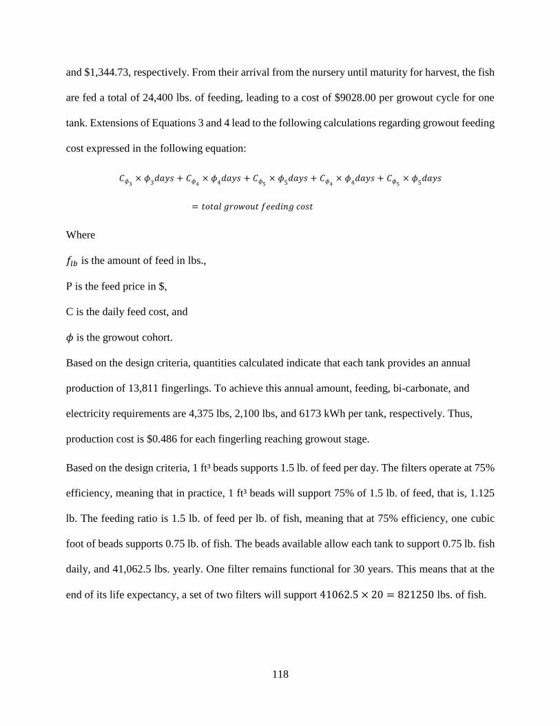
118
and $1,344.73, respectively. From their arrival from the nursery until maturity for harvest, the fish
are fed a total of 24,400 lbs. of feeding, leading to a cost of $9028.00 per growout cycle for one
tank. Extensions of Equations 3 and 4 lead to the following calculations regarding growout feeding
cost expressed in the following equation:
𝐶𝜙3× 𝜙
3𝑑𝑎𝑦𝑠 + 𝐶𝜙4
× 𝜙4
𝑑𝑎𝑦𝑠 + 𝐶𝜙5× 𝜙
5𝑑𝑎𝑦𝑠 + 𝐶𝜙4
× 𝜙4𝑑𝑎𝑦𝑠 + 𝐶𝜙5
× 𝜙5𝑑𝑎𝑦𝑠
= 𝑡𝑜𝑡𝑎𝑙 𝑔𝑟𝑜𝑤𝑜𝑢𝑡 𝑓𝑒𝑒𝑑𝑖𝑛𝑔 𝑐𝑜𝑠𝑡
Where
𝑓𝑙𝑏 is the amount of feed in lbs.,
Ρ is the feed price in $,
C is the daily feed cost, and
𝜙 is the growout cohort.
Based on the design criteria, quantities calculated indicate that each tank provides an annual
production of 13,811 fingerlings. To achieve this annual amount, feeding, bi-carbonate, and
electricity requirements are 4,375 lbs, 2,100 lbs, and 6173 kWh per tank, respectively. Thus,
production cost is $0.486 for each fingerling reaching growout stage.
Based on the design criteria, 1 ft³ beads supports 1.5 lb. of feed per day. The filters operate at 75%
efficiency, meaning that in practice, 1 ft³ beads will support 75% of 1.5 lb. of feed, that is, 1.125
lb. The feeding ratio is 1.5 lb. of feed per lb. of fish, meaning that at 75% efficiency, one cubic
foot of beads supports 0.75 lb. of fish. The beads available allow each tank to support 0.75 lb. fish
daily, and 41,062.5 lbs. yearly. One filter remains functional for 30 years. This means that at the
end of its life expectancy, a set of two filters will support 41062.5 × 20 = 821250 lbs. of fish.
119
The cost for operating fingerling tanks and caring for the fingerlings is largely made up of the
feeding cost and the cost of chemicals for 112 days. Through the fingerling cycle, the fish are
administered feeding at a ratio of 1.4 lb. of feeding per lb. of fish, feeding being priced at $0.37/lb.
Thus, to complete a fingerling cycle, it therefore costs, in terms of feeding,
$840.14 to feed 7500 fish
$0.11 to feed one fish
$840.14 to feed 1621.43 lbs. of fish (2270.84 lbs. of feeding divided by 1.4, 1.4 lb. to 1
lb. being the feed/fish weight ratio)
$0.52 to feed 1 lb. of fish
The chemical compound is priced at $0.40 per lb. knowing that 0.24 lb. is required per lb. of feed.
Cost values are obtained by multiplying feed amounts by 0.24 lb. × $0.40 = 0.096.

120
Appendix F: Annual Breakdown of Life Cycle Cost
Table 27: Life-cycle cost for one tank
Air TUBEBackwash
Blowers
Piping PVC +
fittingsTank Box Truck Stock Feed Chemical Electricity Labor Transport Heating
Greenhouse
Purge Building
Metal Building
Office &
Storage
Greenhouse
Growout Maintenance Total Cost
17,200.00$ 175.00$ 2,000.00$ 57,190.00$ 20,000.00$ 6,102.14$ 20,881.88$ 7,224.00$ 3,254.83$ 45,000.00$ 375.00$ 2,000.00$ 80,000.00$ $ 24,500.00 $ 160,000.00 $ - $ 458,508.90
-$ -$ -$ -$ -$ 6,102.14$ 20,881.88$ 7,224.00$ 3,254.83$ 45,000.00$ 375.00$ 2,000.00$ -$ -$ -$ 5,000.00$ $ 89,837.85
-$ -$ -$ -$ -$ 6,102.14$ 20,881.88$ 7,224.00$ 3,254.83$ 45,000.00$ 375.00$ 2,000.00$ -$ -$ -$ 5,000.00$ $ 89,837.85
-$ -$ -$ -$ -$ 6,102.14$ 20,881.88$ 7,224.00$ 3,254.83$ 45,000.00$ 375.00$ 2,000.00$ -$ -$ -$ 5,000.00$ $ 89,837.85
-$ -$ -$ -$ -$ 6,102.14$ 20,881.88$ 7,224.00$ 3,254.83$ 45,000.00$ 375.00$ 2,000.00$ -$ -$ -$ 5,000.00$ $ 89,837.85
-$ -$ 2,000.00$ -$ -$ 6,102.14$ 20,881.88$ 7,224.00$ 3,254.83$ 45,000.00$ 375.00$ 2,000.00$ -$ -$ -$ 5,000.00$ $ 91,837.85
-$ -$ -$ -$ -$ 6,102.14$ 20,881.88$ 7,224.00$ 3,254.83$ 45,000.00$ 375.00$ 2,000.00$ -$ -$ -$ 5,000.00$ $ 89,837.85
-$ -$ -$ -$ -$ 6,102.14$ 20,881.88$ 7,224.00$ 3,254.83$ 45,000.00$ 375.00$ 2,000.00$ -$ -$ -$ 5,000.00$ $ 89,837.85
-$ -$ -$ -$ -$ 6,102.14$ 20,881.88$ 7,224.00$ 3,254.83$ 45,000.00$ 375.00$ 2,000.00$ -$ -$ -$ 5,000.00$ $ 89,837.85
-$ -$ -$ -$ -$ 6,102.14$ 20,881.88$ 7,224.00$ 3,254.83$ 45,000.00$ 375.00$ 2,000.00$ -$ -$ -$ 5,000.00$ $ 89,837.85
17,200.00$ 175.00$ 2,000.00$ -$ -$ 6,102.14$ 20,881.88$ 7,224.00$ 3,254.83$ 45,000.00$ 375.00$ 2,000.00$ -$ -$ -$ 5,000.00$ $ 111,068.90
-$ -$ -$ -$ -$ 6,102.14$ 20,881.88$ 7,224.00$ 3,254.83$ 45,000.00$ 375.00$ 2,000.00$ -$ -$ -$ 5,000.00$ $ 89,837.85
-$ -$ -$ -$ -$ 6,102.14$ 20,881.88$ 7,224.00$ 3,254.83$ 45,000.00$ 375.00$ 2,000.00$ -$ -$ -$ 5,000.00$ $ 89,837.85
-$ -$ -$ -$ -$ 6,102.14$ 20,881.88$ 7,224.00$ 3,254.83$ 45,000.00$ 375.00$ 2,000.00$ -$ -$ -$ 5,000.00$ $ 89,837.85
-$ -$ -$ -$ -$ 6,102.14$ 20,881.88$ 7,224.00$ 3,254.83$ 45,000.00$ 375.00$ 2,000.00$ -$ -$ -$ 5,000.00$ $ 89,837.85
-$ -$ 2,000.00$ -$ 20,000.00$ 6,102.14$ 20,881.88$ 7,224.00$ 3,254.83$ 45,000.00$ 375.00$ 2,000.00$ -$ -$ -$ 5,000.00$ $ 111,837.85
-$ -$ -$ -$ -$ 6,102.14$ 20,881.88$ 7,224.00$ 3,254.83$ 45,000.00$ 375.00$ 2,000.00$ -$ -$ -$ 5,000.00$ $ 89,837.85
-$ -$ -$ -$ -$ 6,102.14$ 20,881.88$ 7,224.00$ 3,254.83$ 45,000.00$ 375.00$ 2,000.00$ -$ -$ -$ 5,000.00$ $ 89,837.85
-$ -$ -$ -$ -$ 6,102.14$ 20,881.88$ 7,224.00$ 3,254.83$ 45,000.00$ 375.00$ 2,000.00$ -$ -$ -$ 5,000.00$ $ 89,837.85
-$ -$ -$ -$ -$ 6,102.14$ 20,881.88$ 7,224.00$ 3,254.83$ 45,000.00$ 375.00$ 2,000.00$ -$ -$ -$ 5,000.00$ $ 89,837.85
17,200.00$ 175.00$ 2,000.00$ 57,190.00$ -$ 6,102.14$ 20,881.88$ 7,224.00$ 3,254.83$ 45,000.00$ 375.00$ 2,000.00$ 80,000.00$ 24,500.00$ 160,000.00$ 5,000.00$ $ 443,508.90
68,800.00$ 700.00$ 14,000.00$ 114,380.00$ 40,000.00$ 189,166.47$ 647,338.13$ 223,944.00$ 100,899.63$ 1,395,000.00$ 11,625.00$ 62,000.00$ 160,000.00$ 49,000.00$ 320,000.00$ 150,000.00$ 3,575,777.44$
121
Appendix G: Greenhouse Heating Requirements
Heat requirement calculations are based on heat loss data that helps predict heating loads. Jones
(2010) provided a heat loss equation by conduction:
Q = U A (Ti - To)
Where:
Q = heat transfer rate in BTU/hr.
U = heat transfer coefficient in BTU/hr.-ft2 °F (1/R value)
A = surface area in ft2
Ti - To = air temperature difference between inside and outside in °F.
"U" values are sometimes substitutes for "R" values (resistance to heat flow), but Jones (2010)
noted that the relation between "U" and "R" was: U = 1/R.
Jones (2010) also provided a complementary editable Excel spreadsheet that we edited by
entering input from our proposed facility’s buildings’ data. The edited spreadsheet is presented in
the following table:
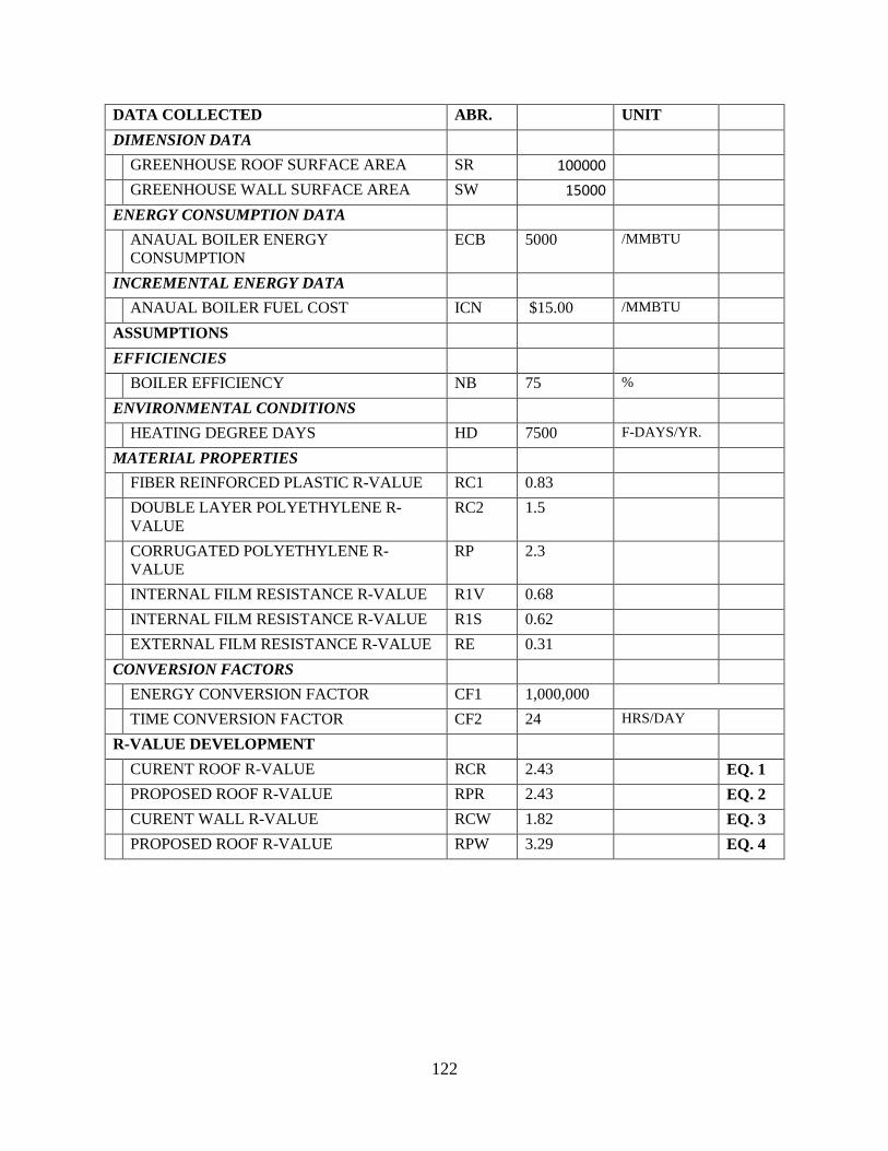
122
DATA COLLECTED ABR. UNIT
DIMENSION DATA
GREENHOUSE ROOF SURFACE AREA SR 100000
GREENHOUSE WALL SURFACE AREA SW 15000
ENERGY CONSUMPTION DATA
ANAUAL BOILER ENERGY
CONSUMPTION
ECB 5000 /MMBTU
INCREMENTAL ENERGY DATA
ANAUAL BOILER FUEL COST ICN $15.00 /MMBTU
ASSUMPTIONS
EFFICIENCIES
BOILER EFFICIENCY NB 75 %
ENVIRONMENTAL CONDITIONS
HEATING DEGREE DAYS HD 7500 F-DAYS/YR.
MATERIAL PROPERTIES
FIBER REINFORCED PLASTIC R-VALUE RC1 0.83
DOUBLE LAYER POLYETHYLENE R-
VALUE
RC2 1.5
CORRUGATED POLYETHYLENE R-
VALUE
RP 2.3
INTERNAL FILM RESISTANCE R-VALUE R1V 0.68
INTERNAL FILM RESISTANCE R-VALUE R1S 0.62
EXTERNAL FILM RESISTANCE R-VALUE RE 0.31
CONVERSION FACTORS
ENERGY CONVERSION FACTOR CF1 1,000,000
TIME CONVERSION FACTOR CF2 24 HRS/DAY
R-VALUE DEVELOPMENT
CURENT ROOF R-VALUE RCR 2.43 EQ. 1
PROPOSED ROOF R-VALUE RPR 2.43 EQ. 2
CURENT WALL R-VALUE RCW 1.82 EQ. 3
PROPOSED ROOF R-VALUE RPW 3.29 EQ. 4
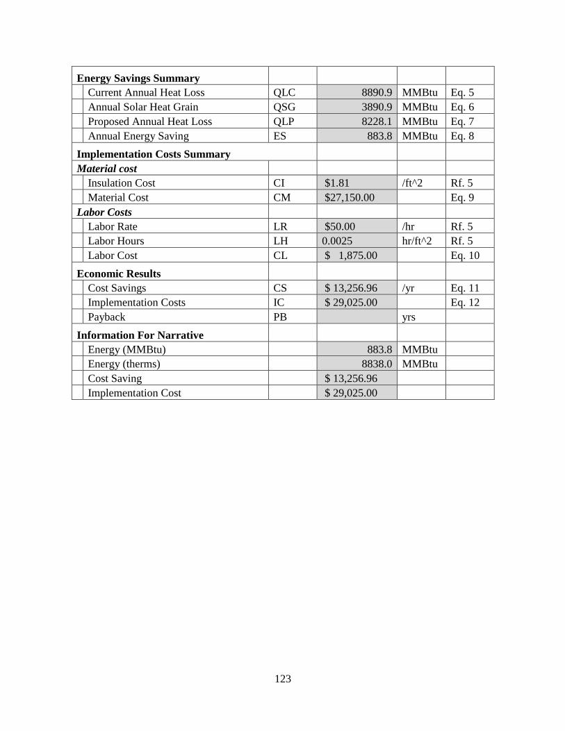
123
Energy Savings Summary
Current Annual Heat Loss QLC 8890.9 MMBtu Eq. 5
Annual Solar Heat Grain QSG 3890.9 MMBtu Eq. 6
Proposed Annual Heat Loss QLP 8228.1 MMBtu Eq. 7
Annual Energy Saving ES 883.8 MMBtu Eq. 8
Implementation Costs Summary
Material cost
Insulation Cost CI $1.81 /ft^2 Rf. 5
Material Cost CM $27,150.00 Eq. 9
Labor Costs
Labor Rate LR $50.00 /hr Rf. 5
Labor Hours LH 0.0025 hr/ft^2 Rf. 5
Labor Cost CL $ 1,875.00 Eq. 10
Economic Results
Cost Savings CS $ 13,256.96 /yr Eq. 11
Implementation Costs IC $ 29,025.00 Eq. 12
Payback PB yrs
Information For Narrative
Energy (MMBtu) 883.8 MMBtu
Energy (therms) 8838.0 MMBtu
Cost Saving $ 13,256.96
Implementation Cost $ 29,025.00

124
The above equations from Oregon State University Energy Efficiency Reference (2014) show
the application of the heat requirement calculations in a sample automatic, computer-generated
professional report.
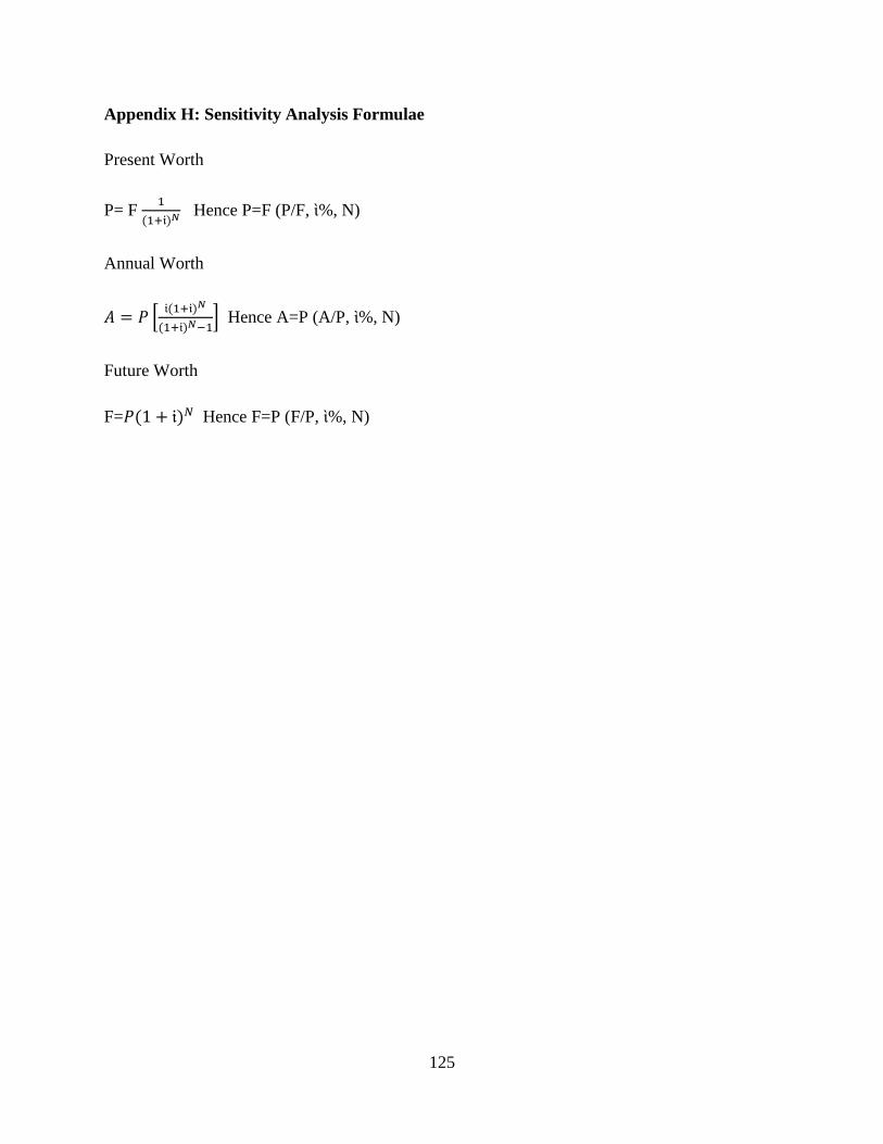
125
Appendix H: Sensitivity Analysis Formulae
Present Worth
P= F 1
(1+𝔦)𝑁 Hence P=F (P/F, ὶ%, N)
Annual Worth
𝐴 = 𝑃 [𝔦(1+𝔦)𝑁
(1+𝔦)𝑁−1] Hence A=P (A/P, ὶ%, N)
Future Worth
F=𝑃(1 + 𝔦)𝑁 Hence F=P (F/P, ὶ%, N)
126
Vita
Marlon Alberetos Greensword was born in 1979 in Spanish Town, Jamaica. He pursued his
elementary education in Kitson Town All-Age School, and his secondary education at St. Catherine
High School and St. Jago High School in Jamaica, where he received his high-school diploma. In 1998,
he obtained a track-and-field scholarship to Gardner Webb University in Boiling Springs, North
Carolina, where he majored in education. A year and a half later, he transferred to Louisiana State
University, where he pursued his athletic activities while majoring in general studies. He obtained a
Bachelor of Arts degree in general studies with concentrations in history, economics, and mechanical
engineering in spring 2005. He then pursued another bachelor’s degree in industrial engineering at
Louisiana State University, which he received in fall 2007, followed by a Master of Science in the
same department in summer 2010. He is now a Ph.D. candidate at the department of Civil and
Environmental Engineering at Louisiana State University.

![Compact ink recirculation system CC1 - Toshiba Tec Top Page...Compact ink recirculation system Example: Mounting of ink recirculation system [CC1] with ink recirculation head Up to](https://img.pdfslide.us/doc/110x75/5f0f72527e708231d4443441/compact-ink-recirculation-system-cc1-toshiba-tec-top-page-compact-ink-recirculation.jpg)