Lie symmetry analysis of the Hanta-epidemic systems

Available online at www.isr-publications.com/jmcsJ. Math. Computer Sci., 17 (2017), 332–344

Research Article

Journal Homepage: www.tjmcs.com - www.isr-publications.com/jmcs

Lie symmetry analysis of the Hanta-epidemic systems

Mevlude Yakit Onguna,∗, Mehmet Kocabiyikb

aSuleyman Demirel University, Department of Mathematics, Isparta, Turkey.bSuleyman Demirel University, Graduate School of Natural and Applied Sciences, Isparta, Turkey.

AbstractWe consider a model for the fatal Hanta-virus infection among mice. Lie symmetry analysis is applied to find general

solutions to Hanta-virus model, which is also known as Abramson-Kenkre model. Besides the solution for the version withderivatives of fractional order, we investigate the model also by using the Lie symmetry method. The basic point of view forboth situations will be logistic differential equation, created for total population. c©2017 All rights reserved.

Keywords: Lie symmetries, logistic differential equation, Hanta epidemics, fractional order differential equation.2010 MSC: 34A05, 34C14, 92D30.

1. Introduction

Hanta-virus causes a fatal contagious disease spreading among mice and the reason for being fatal isthe fact that the viruses genetically contain one chain RNA. This virus has various types, and has been firstdiscovered in South Korea in Hanta river. In this article, Abramson-Kenkre mathematical model [2] willbe used to examine, understand and analyze Hanta-virus dynamics better. This model takes into accountthe spatial and temporal characteristics of Hanta-virus infection. Allen et al. [4] suggested an ordinary-differential-equation model for virus infection. Allen et al. [5] developed two new models for Hanta-virusinfections among male and female rodents. Abramson-Kenkre model is a system of nonlinear differentialequations that defines virus transition from infected mice to susceptible ones. This model, defined bypartial differential equation in Abramson et al. [3], separates the whole mice population in two groups:susceptible and infected.

There is a version of Hanta-virus infection model with ordinary derivatives [2, 4], in the form

dMs

dt= b(Ms +Mi) − cMs −

Ms(Ms +Mi)

K− aMsMi, (1.1)

dMi

dt= −cMi −

Mi(Ms +Mi)

K+ aMsMi, (1.2)

where

∗Corresponding authorEmail addresses: [email protected] (Mevlude Yakit Ongun), [email protected] (Mehmet Kocabiyik)

doi:10.22436/jmcs.017.02.16

Received 2016-08-24

http://dx.doi.org/10.22436/jmcs.017.02.16

M. Y. Ongun, M. Kocabiyik, J. Math. Computer Sci., 17 (2017), 332–344 333

Ms: Mice population without disease;Mi: Mice population with disease;a: infection rate;b: birth rate;c: death rate;K: Environment contagion capacity.

In this model, the infection process is ignored, and the whole population is split into two groups: sensitivemice and mice with disease.

In system (1.1) and (1.2), if M =Ms +Mi is the total population, then

dM

dt= (b− c)M−

M2

K, (1.3)

so we obtain the logistic differential equation. In the next phases of this article, with the use of gen-eral solution of logistic differential equation with Lie symmetry method, we will calculate Ms and Mi

populations. Besides, the version of the Hanta-virus model with derivatives of fractional order is

DαtMs = b(Ms +Mi) − cMs −Ms(Ms +Mi)

K− aMsMi, (1.4)

DαtMi = −cMi −Mi(Ms +Mi)

K+ aMsMi, (1.5)

where Dαt denotes the fractional derivative operator with respect to the origin, according to Caputo’s def-inition [29]. Ms(t) and Mi(t) are the activator and inhibitor variables, respectively. Fractional derivativesare used to describe non-homogeneous character of ecosystems, with respect to presence of competitors.The parameter α denotes the density of competitor species in the systems [1]. When 0 < α < 1, competitorpopulation varies, and for α > 1, it increases.

These are some suggestions about the solution of Hanta epidemic model [1, 3, 9, 10, 15, 18–20, 24, 30,33, 34].

This paper is organized as follows: in Section 2, we define some basic definitions and theoremsrelated with Lie symmetry transformation. Section 3 includes basic concepts and prolongation formulafor fractional-order differential equations. In Section 4, we find general solutions of the Hanta-virusmodel, both of ordinary and fractional orders. The results are illustrated by some graphics and figures.

2. Basic definitions and concepts

For this section, these are the important books and papers about Lie groups and Lie symmetry trans-formation: [7, 8, 11–14, 16, 21–23, 27, 28, 32].

2.1. Lie groups with one parameterLet

φ : R2 × a→ R, ψ : R2 × a→ R,

where for all a ∈ R, the parameters φ and ψ are analytical functions

φ(x,y,a) = x1, and ψ(x,y,a) = y1, (2.1)

and using Ta : R2 → R2

(x,y)→ Ta(x,y) = (φ(x,y,a),ψ(x,y,b)) = (x1,y1),

the set

G = [Ta| a ∈ R], (2.2)

will be defined. If the set (2.2) satisfies the group axioms, then it is named as one-parameter Lie group.The functions φ and ψ in the definition of Lie are named as global form of group (finite form). If we take


an arbitrary point (x,y) and expand (2.1) in the Taylor series about a = 0, we obtain

x1 = x+ aξ(x,y) + 0(a2),

y1 = y+ aη(x,y) + 0(a2),

which is named infinitesimal transformations of the Lie group transformations, and ξ and η are infinites-imals of the group and are defined by [27]

ξ(x,y) = (∂x1

∂a)a=0,

η(x,y) = (∂y1

∂a)a=0.

We can use differential operator

L = ξ(x,y)∂

∂x+ η(x,y)

∂

∂y,

to observe a smooth function change under the influence of an infinitesimal. The operator L is called aninfinitesimal generator of Lie group or the Lie operator.

2.2. Canonical form and variablesIf ξ(x,y) = 0 and η(x,y) = 0, then (x,y) will be a fixed point under the influence of infinitesimal

transformation, so it will be fixed under the influence of all variables of the group. These points are calledabsolute invariant points.

Theoretically, it is always possible to find a variable transformation which can transform a parametr-ized Lie group operator in any wanted structure. Especially, to reduce the Lie operator the translationalong y axis which means that the equations that will be integrated; when the operator has the form

L =∂

∂ythen

ξ∂x∂x

+∂x∂y

= 0, (2.3)

ξ∂y∂x

+∂y∂y

= 1. (2.4)

The Lie operator in the form L=∂

∂yis called the operator in canonical form, and the variables which

reduce it to this form are called canonical variables. Every Lie operator L=∂

∂ycan be reduced to the

canonical formdx

ξ=dy

η. (2.5)

To find the canonical variables, we should solve first-order differential equation (2.5) and we should solveequations (2.3) and (2.4), [1–16, 20–23, 26–29, 33].

2.3. Solution of the ordinary differential equations of the first degree by using transformation of Lie symmetryTo set the conditions of symmetry for ordinary differential equations of the first order, we consider

y ′ = f(x,y). (2.6)

As known, symmetry transformations leave new coordinates of differential equations without changingthem. So,

Tε : (x,y)→ (x1,y1) = (x1(x,y, ε), y1(x,y, ε)), ε ∈ R. (2.7)

Transformation (2.7) is symmetry for the equation; in that case it is called symmetry condition for the


equation given by

dy1

dx1= f(x1,y1).

To make this condition more useful, Dx is taken to show total derivative in x direction,

Dx = ∂x + y′∂y + y

′′∂y ′ + · · · .

So, for equation (2.6) symmetry condition will be (2.8)

dy1

dx1=Dxy1

Dxx1=y1x + y

′y1y

x1x + y ′x1y,

and

y1x + y′y1y

x1x + y ′x1y= f(x1,y1). (2.8)

Now let us consider an orbit for an (x,y) point which is non-invariant. If we write, together for an orbiton (x1,y1), the tangent vector under the Lie groups influence,

dx1

dε= ξ(x1,y1),

dy1

dε= η(x1,y1),

and for x1 and y1 Taylor series expansion with the given symmetry condition under the influence y ′ =f(x,y), we will have the following ordinary differential equations linearized symmetry condition

ηx + (ηy − ξx)f− ξyf2 = ξfx + ηfy. (2.9)

2.4. Canonical coordinates for ordinary differential equations of the first degree.Let assume that we can find non-trivial symmetries for ordinary differential equation (2.6); these sym-

metries include translational Lie group in y-direction. Our main aim here is to pass to new coordinateswith the help of symmetry transformations of differential equation (2.6). These new coordinates will leadus to a new differential equation which includes translations directed to the dependent variable. Thesenew coordinates are called canonical coordinates. In this direction, we have

(r, s) = (r(x,y), s(x,y)), rxsy − rysx 6= 0, (2.10)

If we take new coordinates which are given in (2.10), for the considered new coordinates, with the use ofordinary differential equation and chain rule on tangent vector on (r, s) point, the result will be

ξ(x,y)rx + η(x,y)ry = 0, ξ(x,y)sx + η(x,y)sy = 1, (2.11)

where (r, s) satisfies(i) if ξ 6= 0 an integral of differential equation

dy

dx=η(x,y)ξ(x,y)

can be found easily. The first integral of the above ordinary differential equation will be

φ(x,y) = c, φy 6= 0,

and

r = φ(x,y), s =

(∫dx

ξ(x,y(x, r))

)|r=r(x,y) .


(ii) If ξ = 0 (if these symmetries are not trivial ones, then η = 0). From the first equation of (2.11), we cansee that ry = 0. Simply we can find the canonical coordinates:

r = x, and s =

(∫dy

η(r,y)

)|r=x .

So, by the help of canonical coordinates, the general solution of the ordinary differential equation (2.6)

will be (ds

dr= Ω(r, s))

s(x,y) −∫r(x,y)

Ω(r)dr+ c = 0.

3. Fractional Lie symmetry

3.1. Basic concept and definitions for fractional-order differential equationsSome books and studies that we can use as the basis for fractional-order differential equations are

[6, 17, 18, 25, 26, 29, 31]. Let us consider the differential equation with fractional derivative of order α.

Dαxy(x) = f(x,y).

First, we will consider the Riemann-Liouville fractional derivative operator, that can be defined by

Dαxy(x) =1

Γ(1 −α)

d

dx

∫x0

y(t)

(x− t)αdt, (3.1)

where Γ(.) is the Gamma function.The Caputo fractional derivative operator is

Dαxy(x) =1

Γ(1 −α)

∫x0

y ′(t)

(x− t)αdt.

In real-world problems, Caputo derivative is more common since it produces better results with initialand boundary conditions. Here we will use the Leibniz rule for general fractional order [18]

Dαx (f(x)g(x)) =

∞∑n=0

(

(α

n

))Dα−nx f(x)gn(x), α > 0.

In accordance with Lie group theory, we have the following infinitesimal transformation expandings

x1 = x+ aξ(x,y) + 0(a2),

y1 = y+ aη(x,y) + 0(a2),

yn1 = yn(x) + aηn(x,y) + 0(a2),

Dαxy1 = Dαxy+ aηn(x,y) + 0(a2).

With the use of above equations, equation (3.2) will be infinitesimal generator which expanded in ordern,

ηn = D(η(n−1)) − y(n)D(ξ), (3.2)

where D is total derivative operator as defined in the theory of ordinary differential equations. Theformula (3.2) is called prolongation formula.


Having in mind the definition of total derivative D and yn =dny

dxn, (3.2) can be rewritten in the form

ηn = Dn(η− ξy(1)) + ξy(n+1). (3.3)

By using (3.3), we can write the prolongation formula for fractional derivatives of order α:

η(n) = D(α)x (η− ξy(1)) + ξD

(α+1)x y.

Prolongation formula can be easily generalized for fractional equations of order α [17, 18, 21, 25, 28],

ηα = Dαxη+Dαx (Dx(ξ)y) + ξD

α+1x y−Dα+1

x (ξy).

Considering the infinitesimal generators x1 and y1 given at the beginning, and symmetry group transfor-mation of differential equation of fractional order, the corresponding symmetry condition can be written

(ηα −∂f

∂xξ−

∂f

∂yη)|Dαxy=f(x,y) = 0, (3.4)

where ηα is from the prolongation formula, and, using the general Leibniz rule [18] it can be also writtenas

ηα = Dαxη+

∞∑n=0

(α

n

)n−α

n+ 1Dα−nx yDn+1

x ξ. (3.5)

4. Hanta-virus epidemics with Lie symmetry method

4.1. Hanta-virus epidemics with ordinary orderSumming, side by side, equations (1.1) and (1.2) and using M =Ms +Mi, we get

dM

dt= (b− c)M−

M2

K,

which is the logistic differential equation. From (1.3) and linear symmetry condition, we get tangentvector

(ξ,η) = (1, 0).

Since ξ 6= 0 and using canonical coordinates, we find

r = c, and s = x,

and then, using the solution of corresponding ordinary differential equations, we find the solution

M =K(b− c)e(C1b−C1c+bt−ct)

−1 + e(C1b−C1c+bt−ct), (4.1)

where C1 is an arbitrary constant.Using (1.3), the factM−Mi =Ms, and (4.1), we can rewrite (1.2) in the form of the following ordinary

differential equation for Mi,

dMi

dt= −cMi −

Mi((K(b− c)e(C1b−C1c+bt−ct)

−1 + e(C1b−C1c+bt−ct) −Mi) +Mi)

K(4.2)

+ a(K(b− c)e(C1b−C1c+bt−ct)

−1 + e(C1b−C1c+bt−ct)−Mi)Mi.

From (4.2) and getting into account linear symmetry condition, with the help of the MAPLE 18 and GEM


package program, we we can get the tangent vectors as

(ξ,η) = (0,−(e(tc) − e(C1b−C1c+bt))(−aK)M2i(e

(tc(aK+1))) − e(acKt(C1b−C1c+bt))).

So the solution for Mi will be

Mi =(A

eC1c)aKeC1c

eacKtA(I+C2), (4.3)

where C1 and C2 are arbitrary constants,

A = eC1betb − eC1cetc,

and

I =

∫aeC1c(−Ae−C1c)aK

eacKtdt.

We will find the solution for Ms with the help of (4.3) and (4.1) like this

Ms =K(b− c)e(C1b−C1c+bt−ct)

−1 + e(C1b−C1c+bt−ct)−

(A

eC1c)aKeC1c

eacKtA(I+C2). (4.4)

So, we proved the following proposition.

Proposition 4.1. Let b > c for k 6b

a(b− c)and k >

b

a(b− c),

(i) The Lie symmetry solution for the total population M =Ms +Mi, of equation (1.3) is given by

M =K(b− c)e(C1b−C1c+bt−ct)

−1 + e(C1b−C1c+bt−ct);

(ii) The solutions for mice populations: Ms without disease and Mi with disease, are

Ms =K(b− c)e(C1b−C1c+bt−ct)

−1 + e(C1b−C1c+bt−ct)−

(A

eC1c)aKeC1c

eacKtA(I+C2),

and

Mi =(A

eC1c)aKeC1c

eacKtA(I+C2),

respectively, where

A = eC1betb − eC1cetc,

and

I =

∫aeC1c(−Ae−C1c)aK

eacKtdt.

4.2. Hanta-virus epidemics model with fractional orderBy a similar procedure as above, from equations (1.4) and (1.5) with derivatives of fractional order, we

can get

DαtM = (b− c)M−M2

K, (4.5)

which is again the logistic differential equation, where M = Mi +Ms. The corresponding symmetry


condition is

ηα − η((b− c) −2KM) = 0.

If we choose ξ = ξ(t) and η = p(t)M+ q(t) and using the Leibniz rule for ηα, after some necessarilycomplex procedure, we will get the following D1-D2-D3-D4 determination equations

D1 : Dαt q(t) = (b− c)q(t),

D2 :2

α(b− c)Kq(t) = ξ ′(t),

D3 : −αξ ′(t) = p(t),

D4 : pn(t) +n−α

n+ 1ξ(n+1)(t) = 0,

where n ∈N . If D1 equation is solved by using [25], we will have

q(t) = tα−1Eα,α((b− c)tα)C3,

where C3 is an integral constant and Eα,α(.) is a two parameter Mittag-Leffler function defined by

Eα,β(tα) =

∞∑k=0

tαk

Γ(αk+β).

The Mittag-Leffler function is an extension of the exponential function. When α = 1, the expression forq(t) reduces to (b− c)et .

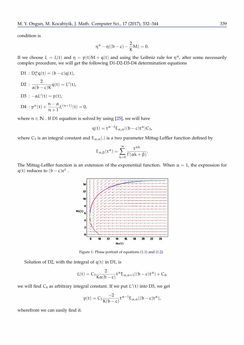
Figure 1: Phase portrait of equations (1.1) and (1.2).

Solution of D2, with the integral of q(t) in D1, is

ξ(t) = C32

Kα(b− c)tαEα,α+1((b− c)t

α) +C4,

we will find C4 as arbitrary integral constant. If we put ξ ′(t) into D3, we get

p(t) = C3−2

K(b− c)tα−1Eα,α((b− c)t

α),

wherefrom we can easily find it.


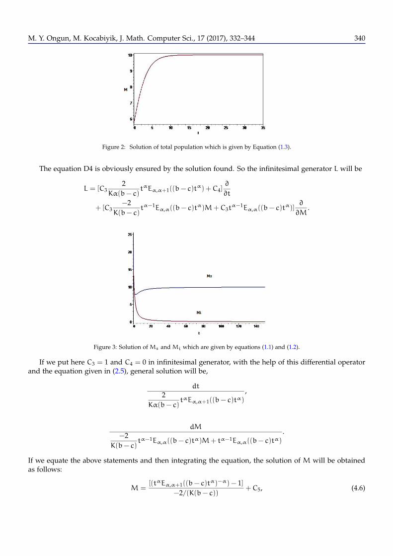
Figure 2: Solution of total population which is given by Equation (1.3).

The equation D4 is obviously ensured by the solution found. So the infinitesimal generator L will be

L = [C32

Kα(b− c)tαEα,α+1((b− c)t

α) +C4]∂

∂t

+ [C3−2

K(b− c)tα−1Eα,α((b− c)t

α)M+C3tα−1Eα,α((b− c)t

α)]∂

∂M.

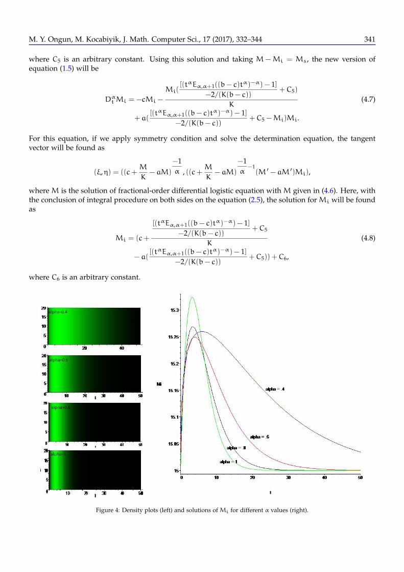
Figure 3: Solution of Ms and Mi which are given by equations (1.1) and (1.2).

If we put here C3 = 1 and C4 = 0 in infinitesimal generator, with the help of this differential operatorand the equation given in (2.5), general solution will be,

dt

2Kα(b− c)

tαEα,α+1((b− c)tα),

dM

−2K(b− c)

tα−1Eα,α((b− c)tα)M+ tα−1Eα,α((b− c)tα).

If we equate the above statements and then integrating the equation, the solution of M will be obtainedas follows:

M =[(tαEα,α+1((b− c)t

α)−α) − 1]−2/(K(b− c))

+C5, (4.6)


where C5 is an arbitrary constant. Using this solution and taking M −Mi = Ms, the new version ofequation (1.5) will be

DαtMi = −cMi −

Mi([(tαEα,α+1((b− c)t

α)−α) − 1]−2/(K(b− c))

+C5)

K(4.7)

+ a([(tαEα,α+1((b− c)t

α)−α) − 1]−2/(K(b− c))

+C5 −Mi)Mi.

For this equation, if we apply symmetry condition and solve the determination equation, the tangentvector will be found as

(ξ,η) = ((c+M

K− aM)

−1α , ((c+

M

K− aM)

−1α

−1(M ′ − aM ′)Mi),

where M is the solution of fractional-order differential logistic equation with M given in (4.6). Here, withthe conclusion of integral procedure on both sides on the equation (2.5), the solution for Mi will be foundas

Mi = (c+

[(tαEα,α+1((b− c)tα)−α) − 1]

−2/(K(b− c))+C5

K(4.8)

− a([(tαEα,α+1((b− c)t

α)−α) − 1]−2/(K(b− c))

+C5)) +C6,

where C6 is an arbitrary constant.

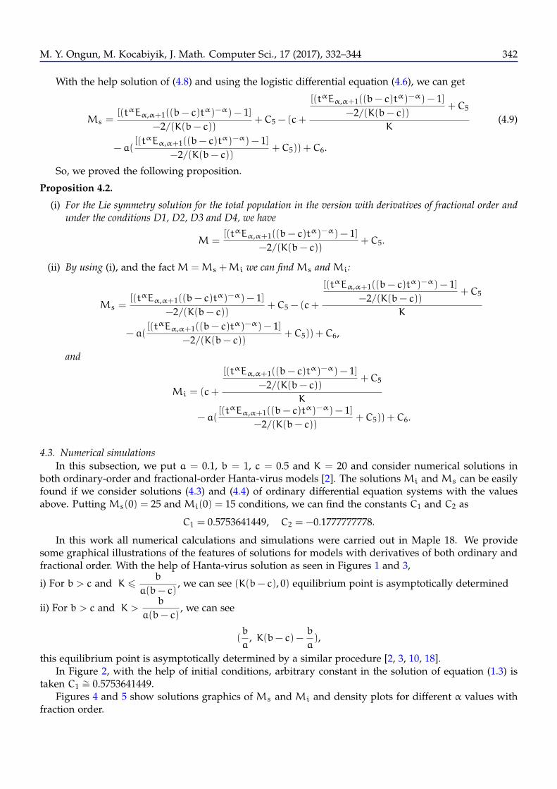
Figure 4: Density plots (left) and solutions of Mi for different α values (right).


With the help solution of (4.8) and using the logistic differential equation (4.6), we can get

Ms =[(tαEα,α+1((b− c)t

α)−α) − 1]−2/(K(b− c))

+C5 − (c+

[(tαEα,α+1((b− c)tα)−α) − 1]

−2/(K(b− c))+C5

K(4.9)


α)−α) − 1]−2/(K(b− c))

+C5)) +C6.

So, we proved the following proposition.

Proposition 4.2.

(i) For the Lie symmetry solution for the total population in the version with derivatives of fractional order andunder the conditions D1, D2, D3 and D4, we have

M =[(tαEα,α+1((b− c)t

α)−α) − 1]−2/(K(b− c))

+C5.

(ii) By using (i), and the fact M =Ms +Mi we can find Ms and Mi:

Ms =[(tαEα,α+1((b− c)t

α)−α) − 1]−2/(K(b− c))

+C5 − (c+

[(tαEα,α+1((b− c)tα)−α) − 1]

−2/(K(b− c))+C5

K


α)−α) − 1]−2/(K(b− c))

+C5)) +C6,

and

Mi = (c+

[(tαEα,α+1((b− c)tα)−α) − 1]

−2/(K(b− c))+C5

K


α)−α) − 1]−2/(K(b− c))

+C5)) +C6.

4.3. Numerical simulationsIn this subsection, we put a = 0.1, b = 1, c = 0.5 and K = 20 and consider numerical solutions in

both ordinary-order and fractional-order Hanta-virus models [2]. The solutions Mi and Ms can be easilyfound if we consider solutions (4.3) and (4.4) of ordinary differential equation systems with the valuesabove. Putting Ms(0) = 25 and Mi(0) = 15 conditions, we can find the constants C1 and C2 as

C1 = 0.5753641449, C2 = −0.1777777778.

In this work all numerical calculations and simulations were carried out in Maple 18. We providesome graphical illustrations of the features of solutions for models with derivatives of both ordinary andfractional order. With the help of Hanta-virus solution as seen in Figures 1 and 3,

i) For b > c and K 6b

a(b− c), we can see (K(b− c), 0) equilibrium point is asymptotically determined

ii) For b > c and K >b

a(b− c), we can see

(b

a, K(b− c) −

b

a),

this equilibrium point is asymptotically determined by a similar procedure [2, 3, 10, 18].In Figure 2, with the help of initial conditions, arbitrary constant in the solution of equation (1.3) is

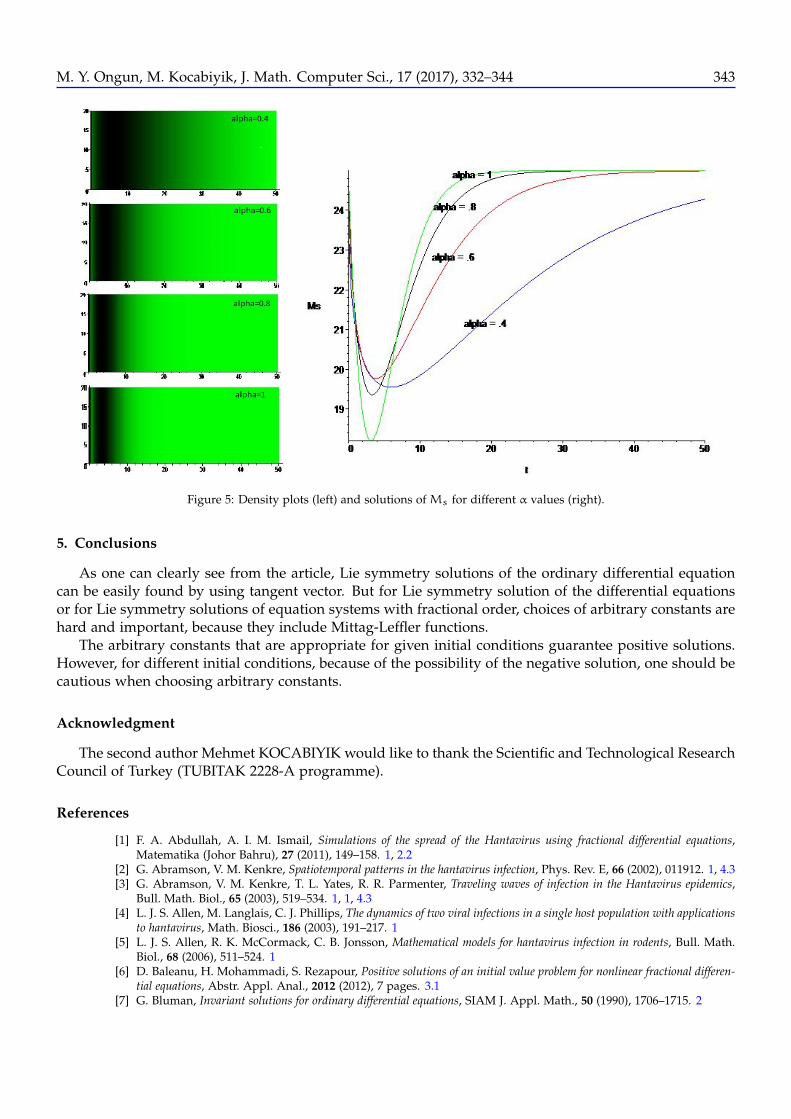
taken C1 ∼= 0.5753641449.Figures 4 and 5 show solutions graphics of Ms and Mi and density plots for different α values with

fraction order.


Figure 5: Density plots (left) and solutions of Ms for different α values (right).

5. Conclusions

As one can clearly see from the article, Lie symmetry solutions of the ordinary differential equationcan be easily found by using tangent vector. But for Lie symmetry solution of the differential equationsor for Lie symmetry solutions of equation systems with fractional order, choices of arbitrary constants arehard and important, because they include Mittag-Leffler functions.

The arbitrary constants that are appropriate for given initial conditions guarantee positive solutions.However, for different initial conditions, because of the possibility of the negative solution, one should becautious when choosing arbitrary constants.

Acknowledgment

The second author Mehmet KOCABIYIK would like to thank the Scientific and Technological ResearchCouncil of Turkey (TUBITAK 2228-A programme).

References

[1] F. A. Abdullah, A. I. M. Ismail, Simulations of the spread of the Hantavirus using fractional differential equations,Matematika (Johor Bahru), 27 (2011), 149–158. 1, 2.2

[2] G. Abramson, V. M. Kenkre, Spatiotemporal patterns in the hantavirus infection, Phys. Rev. E, 66 (2002), 011912. 1, 4.3[3] G. Abramson, V. M. Kenkre, T. L. Yates, R. R. Parmenter, Traveling waves of infection in the Hantavirus epidemics,

Bull. Math. Biol., 65 (2003), 519–534. 1, 1, 4.3[4] L. J. S. Allen, M. Langlais, C. J. Phillips, The dynamics of two viral infections in a single host population with applications

to hantavirus, Math. Biosci., 186 (2003), 191–217. 1[5] L. J. S. Allen, R. K. McCormack, C. B. Jonsson, Mathematical models for hantavirus infection in rodents, Bull. Math.

Biol., 68 (2006), 511–524. 1[6] D. Baleanu, H. Mohammadi, S. Rezapour, Positive solutions of an initial value problem for nonlinear fractional differen-

tial equations, Abstr. Appl. Anal., 2012 (2012), 7 pages. 3.1[7] G. Bluman, Invariant solutions for ordinary differential equations, SIAM J. Appl. Math., 50 (1990), 1706–1715. 2


[8] G. W. Bluman, S. Kumei, Symmetries and Differential Equations, Appl. Math. Sci., 81, Springer-Verlag, New York,(1989). 2

[9] M.-X. Chen, D. P. Clemence, Analysis of and numerical schemes for a mouse population model in hantavirus epidemics, J.Difference Equ. Appl., 12 (2006), 887–899. 1

[10] M.-X. Chen, D. P. Clemence, Stability properties of a nonstandard finite difference scheme for a hantavirus epidemic model,J. Difference Equ. Appl., 12 (2006), 1243–1256. 1, 4.3

[11] A. F. Cheviakov, GeM software package for computation of symmetries and conservation laws of differential equations,Comput. Phys. Comm., 176 (2007), 48–61. 2

[12] A. F. Cheviakov, Computation of fluxes of conservation laws, J. Engrg. Math., 66 (2010), 153–173.[13] A. F. Cheviakov, Symbolic computation of local symmetries of nonlinear and linear partial and ordinary differential equa-

tions, Math. Comput. Sci., 4 (2010), 203–222.[14] A. Cohen, An Introduction tO tHe Lie Theory of One-Parameter Groups; With Applications to the Solution of Differential

Equations, D. C. Heath , Boston, New York, (1911). 2[15] D.-Q. Ding, M. Qiang, X.-H. Ding, A non-standard finite difference scheme for an epidemic model with vaccination, J.

Difference Equ. Appl., 19 (2013), 179–190. 1[16] M. Edwards, M. C. Nucci, Application of Lie group analysis to a core group model for sexually transmitted diseases, J.

Nonlinear Math. Phys., 13 (2006), 211–230. 2, 2.2[17] R. K. Gazizov, A. A. Kasatkin, S. Y. Lukashchuk, Continuous transformation groups of fractional differential equations,

Vestnik UGATU, 9 (2007), 125–135. 3.1, 3.1[18] R. K. Gazizov, A. A. Kasatkin, S. Y. Lukashchuk, Group-invariant solutions of fractional differential equations; in: J. A.

Tenreiro Machado (ed.) et al., Nonlinear Science and Complexity Springer, Berlin, (2011), 51–58. 1, 3.1, 3.1, 3.1, 3.1,4.3

[19] S. M. Goh, A. I. M. Ismail, M. S. M. Noorani, I. Hashim, Dynamics of the hantavirus infection through variationaliteration method, Nonlinear Anal. Real World Appl., 10 (2009), 2171–2176.

[20] A. Gokdogan, M. Merdan, A. Yildirim, A multistage differential transformation method for approximate solution ofHantavirus infection model, Commun. Nonlinear Sci. Numer. Simul., 17 (2012), 1–8. 1, 2.2

[21] P. E. Hyden, Symmetry Methods for Differential Equations. A Beginner’s Guide, Cambridge Texts Appl. Math, Cam-bridge University Press, Cambridge, (2000). 2, 3.1

[22] N. H. Ibragimov, Selected Works, Vol. 1, 2, Karlskrona, Sweden: Alga Publications, Blekinge Institute of Technology,(2001).

[23] N. H. Ibragimov, M. C. Nucci, Integration of third order ordinary differential equations by Lie’s method: equationsadmitting three-dimensional Lie algebras, Lie Groups Appl., 1 (1994), 49–64 . 2, 2.2

[24] Z. G. Karadem, M. Yakıt Ongun, Logistic differential equations obtained from Hanta-virus model, (in Turkish) FenDerg., 11 (2016), 82–91. 1

[25] A. A. Kilbas, H. M. Srivastava, J. J. Trujillo, Theory and Applications of Fractional Differential Equations, North-HollandMath. Stud., Elsevier, Amsterdam, (2006). 3.1, 3.1, 4.2

[26] B. K. Oldham, J. Spainer, The Fractional Calculus. Theory and Applications of Differentiation and Integration to ArbitraryOrder, Math. Sci. Eng, 111, Academic Press , New York–London, (1974). 2.2, 3.1

[27] P. J. Oliver, Applications of Lie Groups to Differential Equations, Grad. Texts Math., 107, Springer-Verlag, New York,(1986). 2, 2.1

[28] L. V. Ovsiannikov, Group Analysis of Differential Equations, Academic Press, New York–London, (1982). 2, 3.1[29] I. Podlubny, Fractional Differential Equations, An Introduction to Fractional Derivatives, Fractional Differential Equations,

to Methods of Their Solution and Some of Their Applications, Math. Sci. Eng., Academic Press, San Diego, CA, (1999).1, 2.2, 3.1

[30] S. Z. Rida, A. A. El Radi, A. Arafa, M. Khalil, The effect of the environmental parameter on the Hantavirus infectionthrough a fractional-order SI model, Int. J. Basic Appl. Sci., 1 (2012), 88–99. 1

[31] S. G. Samko, A. A. Kilbas, O. I. Marichev, Fractional Integrals And Derivatives. Theory and Applications, Gordon andBreach, Yverdon, (1993). 3.1

[32] V. Torrisi, M. C. Nucci, Application of Lie group analysis to a mathematical model which describes HIV transmission; in: J.A. Leslie and T. P. Robart (eds.), The Geometrical Study of Differential Equations, Washington, DC, (2000), Contemp.Math., 285, Amer. Math. Soc., Providence, RI, (2001), 11–20. 2

[33] C. L. Wesley, Discrete-time and continuous-time models with applications to the spread of hantavirus in wild rodent andhuman populations, Diss., Texas Tech, University, (2008). 1, 2.2

[34] S. Yuzbası, M. Sezer, An exponential matrix method for numerical solutions of Hantavirus infection model, Appl. Appl.Math., 8 (2013), 99–115. 1

Documents

Lie symmetry analysis of the Hanta-epidemic systems