Embed Size (px)
Citation preview
symmetryS S
Article
Lie Symmetries of Nonlinear Parabolic-EllipticSystems and Their Application to a TumourGrowth Model
Roman Cherniha 1,* ID , Vasyl’ Davydovych 1 and John R. King 2 ID
1 Institute of Mathematics, National Academy of Sciences of Ukraine, 3, Tereshchenkivs’ka Street,01601 Kyiv, Ukraine; [email protected]
2 School of Mathematical Sciences, University of Nottingham, University Park, Nottingham NG7 2RD, UK;[email protected]
* Correspondence: [email protected]; Tel.: +380-442-352-010
Received: 25 April 2018; Accepted: 14 May 2018; Published: 17 May 2018�����������������
Abstract: A generalisation of the Lie symmetry method is applied to classify a coupled system ofreaction-diffusion equations wherein the nonlinearities involve arbitrary functions in the limit casein which one equation of the pair is quasi-steady but the other is not. A complete Lie symmetryclassification, including a number of the cases characterised as being unlikely to be identified purelyby intuition, is obtained. Notably, in addition to the symmetry analysis of the PDEs themselves,the approach is extended to allow the derivation of exact solutions to specific moving-boundaryproblems motivated by biological applications (tumour growth). Graphical representations of thesolutions are provided and a biological interpretation is briefly addressed. The results are generalisedon multi-dimensional case under the assumption of the radially symmetrical shape of the tumour.
Keywords: lie symmetry classification; exact solution; nonlinear reaction-diffusion system; tumourgrowth model; moving-boundary problem
1. Introduction
It is well-known that nonlinear reaction-diffusion (RD) systems (i.e., systems of second-orderparabolic PDEs with reaction terms) are used to describe various processes in physics, chemistry,biology, ecology, etc. (see, e.g., books [1–4]). Indeed, there are many special cases of such systemsdescribing real world processes, among the most famous being Lotka–Volterra type systems [5,6] andsystems used for modelling the chemical basis of morphogenesis [7] (see, e.g., ref. [2] for details inmodern terminology).
The most common are two-component RD systems of the form
Ut = (D1(U)Ux)x + F(U, V),Vt = (D2(V)Vx)x + G(U, V),
(1)
where U(t, x) and V(t, x) are unknown functions, the nonnegative smooth functions D1(U) and D2(V)
are coefficients of diffusivity (conductivity), and F and G are arbitrary smooth functions describingthe interaction between components U(t, x) and V(t, x). Hereafter the t and x subscripts denotedifferentiation with respect to these variables.
It should be noted that the search of Lie symmetries of RD systems was initiated many years agoand probably paper [8] was the first in this direction. A complete Lie symmetry classification wasdone much later because this problem is much more complicated in comparison with the case of asingle RD equation. In particular, it was necessary to treat separately the cases of constant diffusivities
Symmetry 2018, 10, 171; doi:10.3390/sym10050171 www.mdpi.com/journal/symmetry
Symmetry 2018, 10, 171 2 of 21
(i.e., semilinear equations) and nonconstant (quasilinear) ones. All possible Lie symmetries of (1) withconstant diffusivities were completely described in [9–11]. In the case of nonconstant diffusivities,it has been done in [12,13] (in [14], the result was extended to the multi-component RD systems).
It should be stressed that there are models used to describe real world processes that are based onsingular limits of a RD system (1), namely with D2(V) = 0 or with the Vt term absent. The system (1)with D2(V) = 0 has been used to describe interactions involving species (cells) V, which are not ableto diffuse in space (typical examples include some models for plankton). Some particular resultsabout Lie symmetries of such systems have been recently obtained in [15], however the problem of acomplete Lie symmetry classification is still not solved.
Here, however, we examine the class of systems (1) with the Vt term negligible so that V isgoverned by a quasi-steady equation, i.e.,
Ut = (D1(U)Ux)x + F(U, V),0 = (D2(V)Vx)x + G(U, V).
(2)
Obviously this system is reduced to the form
Ut = (D1(U)Ux)x + F∗(U, V∗),0 = V∗xx + G∗(U, V∗)
(3)
by the Kirchhoff substitution for the component V → V∗. Here the diffusivity D1(U) is a nonnegativeand nonconstant function (at least in some domains) in what follows. We remind the reader thatthe case D1(U) = const was studied in [9,10]. Thus, the class of parabolic-elliptic systems (3) withD1(U) 6= const is the main object of this study. The main motivation for this follows from paper [16],in which a model for tumour growth was derived. Under some biologically motivated assumptions(see p. 570 in [16] for details), the model was simplified to a boundary-value problem with governingequations of the form (3). System (2) is of course potentially of relevance to any two-component RDmodel in which one species diffuses much faster than the other; it is also of interest purely from thesymmetry point of view, since its symmetries differ essentially from those of (1).
The paper is organized as follows. Section 2 is devoted to the search for form-preservingtransformations for the class of systems (3) in order to establish possible relations between RD systemsthat admit equivalent Lie symmetry algebras. Section 3 is devoted to the identification of all possibleLie symmetries that any system of the form (3) can admit. The main results of this section are presentedin the form of Tables 1 and 2. In Sections 4 and 5, we apply the Lie symmetries derived for the reductionof a nonlinear boundary value problem (BVP) with a free boundary modeling tumour growth in orderto construct its exact solution. Moreover, possible biological interpretations of the results derivedare discussed. Finally, we briefly discuss the result obtained and present some conclusions in thelast section.
2. Form-Preserving Transformations for the Class of Systems (3)
First of all we simplify notations in system (3) in a natural way:
Ut = (D(U)Ux)x + F(U, V),0 = Vxx + G(U, V).
(4)
The class of systems (4) contains three arbitrary functions and the Lie symmetry of its differentrepresentatives depends essentially on the form of the triplet (D, F, G). Thus, the problem of a completedescription of all possible Lie symmetries (the so called group classification problem) arises. In orderto solve this, we can apply the Lie–Ovsiannikov approach (the name of Ovsiannikov arises becausehe published a remarkable paper in this direction, [17]) of the Lie symmetry classification, which isbased on the classical Lie scheme and a set of equivalence transformations of the differential equation
Symmetry 2018, 10, 171 3 of 21
in question. However, it is well-known that this approach leads to a very long list of equations withnontrivial Lie symmetry provided the given equation (system) contains several arbitrary functions(system (4) involves three such).
During the last two decades, new approaches for solving group classification problems weredeveloped, which are important for obtaining the so called canonical list of inequivalent equationsadmitting nontrivial Lie symmetry algebras and allowing the solution of this problem in a more efficientway than a formal application of the Lie–Ovsiannikov approach. Here we use the algorithm based on socalled form-preserving transformations [18,19], which were used initially for finding locally-equivalentPDEs, especially those nonlinear PDEs that are linearizable by a point transformation. Interestingly,such transformations were implicitly used much earlier in [20] in order to find all possible heatequations with nonlinear sources that admit the Lie symmetry either of the linear heat equationor the Burgers equation. In [21], these transformations are called ‘allowed transformations’ andthey were used to classify the Lie symmetries of a class of variable coefficient Korteweg-de Vriesequations. One may say that the above cited paper was the first one, in which allowed (form-preserving)transformations were systematically used for solving the Lie symmetry classification problem. Now wepresent the definition of form-preserving transformations in the case of the class of systems (4).
Definition 1. A point non-degenerate transformation given by the formulae
t = a(τ, y, u, v), x = b(τ, y, u, v),U = ϕ(τ, y, u, v), V = ψ(τ, y, u, v),
(5)
which maps at least one system of the form (4) into a system belonging to the same class, is called aform-preserving transformation.
Comparing this definition with the well-known definition for equivalence transformations,one immediately notes that each equivalence transformation is automatically a form-preservingtransformation, but not vice versa.
It was noted later [22,23] that the form-preserving transformations (nowadays the terminology‘admissible transformations’ is also widely used) allow an essential reduction of the number ofcases obtained via the classical Lie–Ovsiannikov algorithm (see extensive discussions on this matterin [11,13,24]). In particular, it is shown in [13] that there are only 10 inequivalent cases whenRD systems with nonconstant diffusivities and reaction terms of the form (1) are invariant withrespect to the nontrivial Lie algebras (in contrast to a much longer list derived in [12] via theLie–Ovsiannikov algorithm). Similarly, it was proved in [24] that the canonical list of inequivalentreaction-diffusion-convection equations consists of 15 equations only (not the 30 derived by theLie–Ovsiannikov algorithm).
The reader may find more details (including specific examples) on this matter in Section 2.3 of therecent book [25].
Now we present the main result of this section, namely the theorem describing a general form ofform-preserving transformations for the class of systems (4).
Theorem 1. An arbitrary system of the form
uτ =(
D(u)uy)
y + F(u, v),
0 = vyy + G(u, v)(6)
Symmetry 2018, 10, 171 4 of 21
can be reduced to a system from class (4) by a form-preserving transformation of the form (5) if and only if thesmooth functions a, b, ϕ and ψ have the forms
a = α(τ), b = β(τ, y), ατ βy 6= 0,ϕ = K(τ, y)u + P(τ, y), K 6= 0,ψ = L(τ, y)v + Q(τ, y), L 6= 0,
(7)
where the functions α(τ), β(τ, y), K(τ, y), P(τ, y), L(τ, y) and Q(τ, y) are such that the following equalities
ατ D = β2yD,
ατ F = KF +(Kyu+Py)2
K Du + Kτu + Pτ − D(
Kyyu + Pyy − 2 Kyu+PyK Ky
),
β2yG = LG + 2 Lyv+Qy
L Ly − Lyyv−Qyy,2βy(Kyu + Py)Du + D
(2βyKy − βyyK
)+ βτK = 0,
2βyLy − βyyL = 0,
(8)
hold.
The proof of Theorem 1. is quite similar to that for the class of RD systems (1) with Dk = const (k = 1, 2)presented in [26].
The group of equivalence transformations can be easily extracted from Theorem 1 by assumingthat D, F and G are arbitrary smooth functions. Solving the system (8) under such condition onearrives at the following statement.
Consequence 1. The group of equivalence transformations for (4) has the form
t = α1τ + α2, x = α3y + α4,U = α5u + α6, V = α7v + α8,
D =α2
3α1
D, F = α5α1
F, G = α7α2
3G,
(9)
where αl (l = 1, . . . , 8) are arbitrary group parameters (α1 > 0, α2k−1 6= 0, k = 2, 3, 4).
One sees that (8) is a nonlinear system of functional-differential equations and its general solutionseems to be impossible without further restrictions. For example, assuming a constant diffusivity D,one may derive that β(τ, y) is linear with respect to (w.r.t.) the variable y; however, β(τ, y) can benonlinear for the nonconstant diffusivity D (see Tables 3 and 4 below for examples).
While the form of the transformations (7) is still quite general, it will be shown in the next sectionthat only particular cases play important roles in solving the Lie symmetry classification problem forthe nonlinear parabolic-elliptic systems (3).
3. Lie Symmetries of a Class of Parabolic-Elliptic Systems
In order to find Lie symmetry operators of a system of the form (4) via the Lie method [25,27–31],one needs to consider the manifold (S1, S2)
S1 ≡ Ut − (D(U)Ux)x − F(U, V) = 0,S2 ≡ Vxx + G(U, V) = 0
(10)
in the space of the following variables:
t, x, U, V, Ut, Ux, Vt, Vx, Utx, Utt, Uxx, Vtx, Vtt, Vxx.
Symmetry 2018, 10, 171 5 of 21
The system (4) is invariant under the transformations generated by the infinitesimal operator
X = ξ0(t, x, U, V)∂t + ξ1(t, x, U, V)∂x + η1(t, x, U, V)∂U + η2(t, x, U, V)∂V (11)
when the following invariance conditions are satisfied:
X2(S1) ≡ X
2(Ut − (D(U)Ux)x − F(U, V))
∣∣∣S1=0, S2=0
= 0,
X2(S2) ≡ X
2(Vxx + G(U, V))
∣∣∣S1=0, S2=0
= 0.(12)
The operator X2
is the second prolongation of the operator X, i.e.,
X2= X + ρ1
t∂
∂Ut+ ρ1
t∂
∂Vt+ ρ1
x∂
∂Ux+ ρ2
x∂
∂Vx+
σ1tt
∂∂Utt
+ σ1tx
∂∂Utx
+ σ1xx
∂∂Uxx
+ σ2tt
∂∂Vtt
+ σ2tx
∂∂Vtx
+ σ2xx
∂∂Vxx
,(13)
where the coefficients ρ and σ with relevant subscripts are calculated by well-known formulae(see, e.g., [29–31]).
Substituting (13) into (12) and eliminating the derivatives Ut and Vxx using (4), we can obtain thefollowing system of determining equations (DEs):
ξ0x = ξ0
U = ξ0V = ξ1
U = ξ1V = 0, (14)
η1V = η2
U = η2VV = 0, (15)(
2ξ1x − ξ0
t
)D = η1DU, (16)
2η2xV = ξ1
xx, (17)(ξ1
xx − 2η1xU
)D = 2η1
xDU + ξ1t , (18)(
2ξ1x − ξ0
t − η1U
)DU = η1
UUD + η1DUU, (19)
η1FU + η2FV = η1t −Dη1
xx + F(
η1U − ξ0
t
), (20)
η1GU + η2GV = −η2xx + G
(η2
V − 2ξ1x
). (21)
Obviously, the general solution of the above system of DEs essentially depends on the form of thetriplet (D, F, G). Thus, the problem of a complete description of all possible Lie symmetries (the socalled group classification problem) arises.
First of all we find the so called trivial algebra (other terminology used for this algebra isthe ‘principal algebra’ and the ‘kernel of maximal invariance algebras’) of the class in question,i.e., the maximal invariance algebra (MAI) admitted by each equation of the form (4). Under thenatural assumption that D, F and G are arbitrary smooth functions the above system of DEs can beeasily solved and the two-dimensional Lie algebra generated by the basic operators
X1 = ∂t, X2 = ∂x (22)
is obtained.In order to solve the problem of Lie symmetry classification for system (4), i.e., to find all possible
systems admitting three- and higher-dimensional MAI, we use the algorithm based on form-preservingtransformations, which was briefly discussed in Section 2. Moreover, it will be shown below that,similarly to the case of standard nonlinear RD systems [13], such an approach is also more efficient forparabolic-elliptic systems (compared to the classical Lie–Ovsiannikov algorithm).
Symmetry 2018, 10, 171 6 of 21
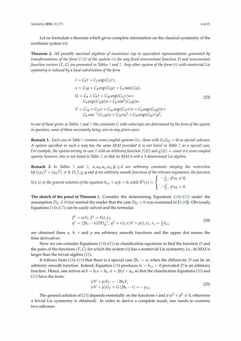
Let us formulate a theorem which gives complete information on the classical symmetry of thenonlinear system (4).
Theorem 2. All possible maximal algebras of invariance (up to equivalent representations generated bytransformations of the form (23)) of the system (4) for any fixed nonconstant function D and nonconstantfunction vectors (F, G) are presented in Tables 1 and 2. Any other system of the form (6) with nontrivial Liesymmetry is reduced by a local substitution of the form
t = C0τ + C1 exp(C2τ),
x = C3y + C4 exp(C5y) + C6 tan(C7y),
U = C8 + C9τ + C10 exp(C11τ)u+C4 exp(C12y)u + C6 cos3(C13y)u,
V = C14 + C15τ + C16 exp(C17τ)v + C4 exp(C12y)v+C6 cos−1(C13y)v + C18τy2 + C19 exp(C20τ)y2,
(23)
to one of those given in Tables 1 and 2 (the constants C with subscripts are determined by the form of the systemin question, some of them necessarily being zero in any given case).
Remark 1. Each case in Table 1 contains semi-coupled systems (i.e., those with FVGU = 0) as special subcases.A system specified in such a way has the same MAI provided it is not listed in Table 2 as a special case.For example, the system arising in case 1 with an arbitrary function f (U) and g(U) = const is a semi-coupledsystem; however, this is not listed in Table 2, so that its MAI is still a 3-dimensional Lie algebra.
Remark 2. In Tables 1 and 2, α, α0, α1, α2, β, γ, k are arbitrary constants obeying the restrictionkβ((α1)
2 + (α2)2) 6= 0; D, f , g, ϕ and ψ are arbitrary smooth functions of the relevant arguments; the function
h(t, x) is the general solution of the equation hxx + α2h = 0, while h0(x) =
−1α2
, if α2 6= 0,
− x2
2 , if α2 = 0.
The sketch of the proof of Theorem 2. Consider the determining Equations (14)–(21) under theassumption DU 6= 0 (we remind the reader that the case DU = 0 was examined in [9,10]). Obviously,Equations (14)–(17) can be easily solved and the formulae
ξ0 = a(t), ξ1 = b(t, x),η1 = (2bx − a)DD−1
U , η2 = r(t, x)V + p(t, x), rx = 12 bxx
(24)
are obtained (here a, b, r and p are arbitrary smooth functions and the upper dot means thetime derivative).
Now we can consider Equations (18)–(21) as classification equations to find the function D andthe pairs of the functions (F, G) for which the system (4) has a nontrivial Lie symmetry, i.e., its MAI islarger than the trivial algebra (22).
It follows from (18)–(19) that there is a special case 2bx = at when the diffusivity D can be anarbitrary smooth function. Indeed, Equation (18) produces bt = bxx = 0 provided D is an arbitraryfunction. Hence, one arrives at b = b1x + b0, a = 2b1t + a0, so that the classification Equations (20) and(21) have the form:
(rV + p)FV = −2b1F,(rV + p)GV + G (2b1 − r) = −pxx.
(25)
The general solution of (25) depends essentially on the functions r and p (r2 + p2 6= 0, otherwisea trivial Lie symmetry is obtained). In order to derive a complete result, one needs to examinetwo subcases.
Symmetry 2018, 10, 171 7 of 21
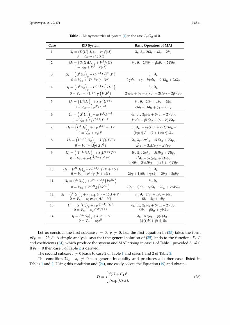
Table 1. Lie symmetries of system (4) in the case FV GU 6= 0.
Case RD System Basic Operators of MAI
1. Ut = (D(U)Ux)x + eV f (U) ∂t, ∂x, 2t∂t + x∂x − 2∂V0 = Vxx + eV g(U)
2. Ut = (D(U)Ux)x + Vβ f (U) ∂t, ∂x, 2βt∂t + βx∂x − 2V∂V0 = Vxx + Vβ+1g(U)
3. Ut =(
UkUx
)x+ Uγ+1 f
(eVUα
)∂t, ∂x,
0 = Vxx + Uγ−kg(eVUα
)2γt∂t + (γ− k)x∂x − 2U∂U + 2α∂V
4. Ut =(
UkUx
)x+ Uγ+1 f
(VUβ
)∂t, ∂x,
0 = Vxx + VUγ−kg(
VUβ)
2γt∂t + (γ− k)x∂x − 2U∂U + 2βV∂V
5. Ut =(
UkUx
)x+ α1eVUγ+1 ∂t, ∂x, 2t∂t + x∂x − 2∂V ,
0 = Vxx + α2eVUγ−k kt∂t −U∂U + (γ− k)∂V
6. Ut =(
UkUx
)x+ α1VβUγ+1 ∂t, ∂x, 2βt∂t + βx∂x − 2V∂V ,
0 = Vxx + α2Vβ+1Uγ−k kβt∂t − βU∂U + (γ− k)V∂V
7. Ut =(
UkUx
)x+ α1Uk+1 + UV ∂t, ∂x, −kϕ(t)∂t + ϕ(t)U∂U+
0 = Vxx + α2Uk (kϕ(t)V + (k + 1)ϕ(t)) ∂V
8. Ut =(
U−4/3Ux
)x+ U f (UV3) ∂t, ∂x, 2x∂x − 3U∂U + V∂V ,
0 = Vxx + Ug(UV3) x2∂x − 3xU∂U + xV∂V
9. Ut =(
U−4/3Ux
)x+ α1U1+γV3γ ∂t, ∂x, 2x∂x − 3U∂U + V∂V ,
0 = Vxx + α2U4/3+γV3γ+1 x2∂x − 3xU∂U + xV∂V ,4γt∂t + 3γU∂U − (4/3 + γ)V∂V
10. Ut =(eUUx
)x + e(γ+1)U f (V + αU) ∂t, ∂x,
0 = Vxx + eγU g (V + αU) 2(γ + 1)t∂t + γx∂x − 2∂U + 2α∂V
11. Ut =(eUUx
)x + e(γ+1)U f
(VeβU
)∂t, ∂x,
0 = Vxx + VeγU g(
VeβU)
2(γ + 1)t∂t + γx∂x − 2∂U + 2βV∂V
12. Ut =(eUUx
)x + α1 exp ((γ + 1)U + V) ∂t, ∂x, 2t∂t + x∂x − 2∂V ,
0 = Vxx + α2 exp (γU + V) t∂t − ∂U + γ∂V
13. Ut =(eUUx
)x + α1e(γ+1)UVβ ∂t, ∂x, 2βt∂t + βx∂x − 2V∂V ,
0 = Vxx + α2eγUVβ+1 βt∂t − β∂U + γV∂V
14. Ut =(eUUx
)x + α1eU + V ∂x, ϕ(t)∂t − ϕ(t)∂U−
0 = Vxx + α2eU (ϕ(t)V + ϕ(t)) ∂V
Let us consider the first subcase r = 0, p 6= 0, i.e., the first equation in (25) takes the formpFV = −2b1F. A simple analysis says that the general solution of (25) leads to the functions F, Gand coefficients (24), which produce the system and MAI arising in case 1 of Table 1 provided b1 6= 0.If b1 = 0 then case 3 of Table 2 is derived.
The second subcase r 6= 0 leads to case 2 of Table 1 and cases 1 and 2 of Table 2.The condition 2bx − at 6= 0 is a generic inequality and produces all other cases listed in
Tables 1 and 2. Using this condition and (24), one easily solves the Equation (19) and obtains
D =
{d(U + C1)
k,
d exp(C2U),(26)
Symmetry 2018, 10, 171 8 of 21
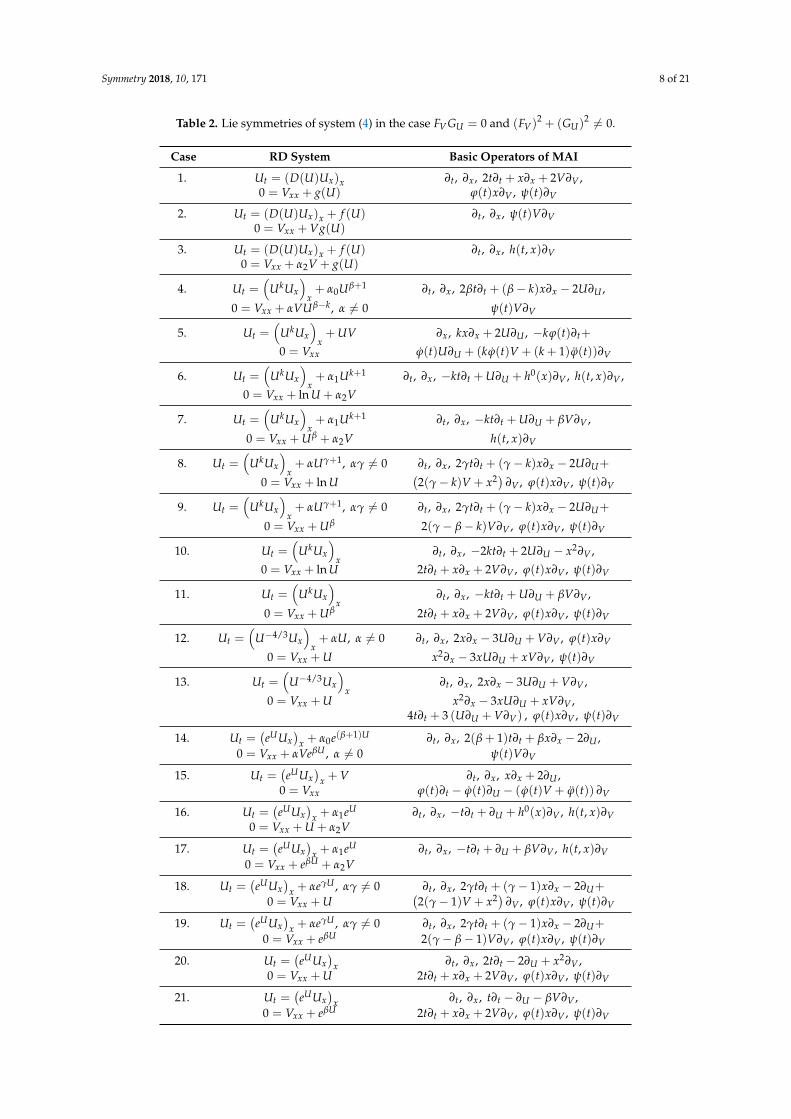
Table 2. Lie symmetries of system (4) in the case FV GU = 0 and (FV)2 + (GU)2 6= 0.
Case RD System Basic Operators of MAI
1. Ut = (D(U)Ux)x ∂t, ∂x, 2t∂t + x∂x + 2V∂V ,0 = Vxx + g(U) ϕ(t)x∂V , ψ(t)∂V
2. Ut = (D(U)Ux)x + f (U) ∂t, ∂x, ψ(t)V∂V0 = Vxx + Vg(U)
3. Ut = (D(U)Ux)x + f (U) ∂t, ∂x, h(t, x)∂V0 = Vxx + α2V + g(U)
4. Ut =(
UkUx
)x+ α0Uβ+1 ∂t, ∂x, 2βt∂t + (β− k)x∂x − 2U∂U ,
0 = Vxx + αVUβ−k, α 6= 0 ψ(t)V∂V
5. Ut =(
UkUx
)x+ UV ∂x, kx∂x + 2U∂U , −kϕ(t)∂t+
0 = Vxx ϕ(t)U∂U + (kϕ(t)V + (k + 1)ϕ(t))∂V
6. Ut =(
UkUx
)x+ α1Uk+1 ∂t, ∂x, −kt∂t + U∂U + h0(x)∂V , h(t, x)∂V ,
0 = Vxx + ln U + α2V
7. Ut =(
UkUx
)x+ α1Uk+1 ∂t, ∂x, −kt∂t + U∂U + βV∂V ,
0 = Vxx + Uβ + α2V h(t, x)∂V
8. Ut =(
UkUx
)x+ αUγ+1, αγ 6= 0 ∂t, ∂x, 2γt∂t + (γ− k)x∂x − 2U∂U+
0 = Vxx + ln U(2(γ− k)V + x2) ∂V , ϕ(t)x∂V , ψ(t)∂V
9. Ut =(
UkUx
)x+ αUγ+1, αγ 6= 0 ∂t, ∂x, 2γt∂t + (γ− k)x∂x − 2U∂U+
0 = Vxx + Uβ 2(γ− β− k)V∂V , ϕ(t)x∂V , ψ(t)∂V
10. Ut =(
UkUx
)x
∂t, ∂x, −2kt∂t + 2U∂U − x2∂V ,
0 = Vxx + ln U 2t∂t + x∂x + 2V∂V , ϕ(t)x∂V , ψ(t)∂V
11. Ut =(
UkUx
)x
∂t, ∂x, −kt∂t + U∂U + βV∂V ,
0 = Vxx + Uβ 2t∂t + x∂x + 2V∂V , ϕ(t)x∂V , ψ(t)∂V
12. Ut =(
U−4/3Ux
)x+ αU, α 6= 0 ∂t, ∂x, 2x∂x − 3U∂U + V∂V , ϕ(t)x∂V
0 = Vxx + U x2∂x − 3xU∂U + xV∂V , ψ(t)∂V
13. Ut =(
U−4/3Ux
)x
∂t, ∂x, 2x∂x − 3U∂U + V∂V ,
0 = Vxx + U x2∂x − 3xU∂U + xV∂V ,4t∂t + 3 (U∂U + V∂V) , ϕ(t)x∂V , ψ(t)∂V
14. Ut =(eUUx
)x + α0e(β+1)U ∂t, ∂x, 2(β + 1)t∂t + βx∂x − 2∂U ,
0 = Vxx + αVeβU , α 6= 0 ψ(t)V∂V
15. Ut =(eUUx
)x + V ∂t, ∂x, x∂x + 2∂U ,
0 = Vxx ϕ(t)∂t − ϕ(t)∂U − (ϕ(t)V + ϕ(t)) ∂V
16. Ut =(eUUx
)x + α1eU ∂t, ∂x, −t∂t + ∂U + h0(x)∂V , h(t, x)∂V
0 = Vxx + U + α2V
17. Ut =(eUUx
)x + α1eU ∂t, ∂x, −t∂t + ∂U + βV∂V , h(t, x)∂V
0 = Vxx + eβU + α2V
18. Ut =(eUUx
)x + αeγU , αγ 6= 0 ∂t, ∂x, 2γt∂t + (γ− 1)x∂x − 2∂U+
0 = Vxx + U(2(γ− 1)V + x2) ∂V , ϕ(t)x∂V , ψ(t)∂V
19. Ut =(eUUx
)x + αeγU , αγ 6= 0 ∂t, ∂x, 2γt∂t + (γ− 1)x∂x − 2∂U+
0 = Vxx + eβU 2(γ− β− 1)V∂V , ϕ(t)x∂V , ψ(t)∂V
20. Ut =(eUUx
)x ∂t, ∂x, 2t∂t − 2∂U + x2∂V ,
0 = Vxx + U 2t∂t + x∂x + 2V∂V , ϕ(t)x∂V , ψ(t)∂V
21. Ut =(eUUx
)x ∂t, ∂x, t∂t − ∂U − βV∂V ,
0 = Vxx + eβU 2t∂t + x∂x + 2V∂V , ϕ(t)x∂V , ψ(t)∂V
Symmetry 2018, 10, 171 9 of 21
where d 6= 0, C1, C2 and k 6= 0 are arbitrary constants. Moreover, substituting (26) into (18),we obtain b = b1x + b0, b0, b1 ∈ R, unless
D = d(U + C1)−4/3, b = b(x). (27)
One notes that the system (4) with diffusivities (26) and (27) can be simplified to one withd = 1, C1 = 0, C2 = 1 by the appropriate equivalence transformations from (9).
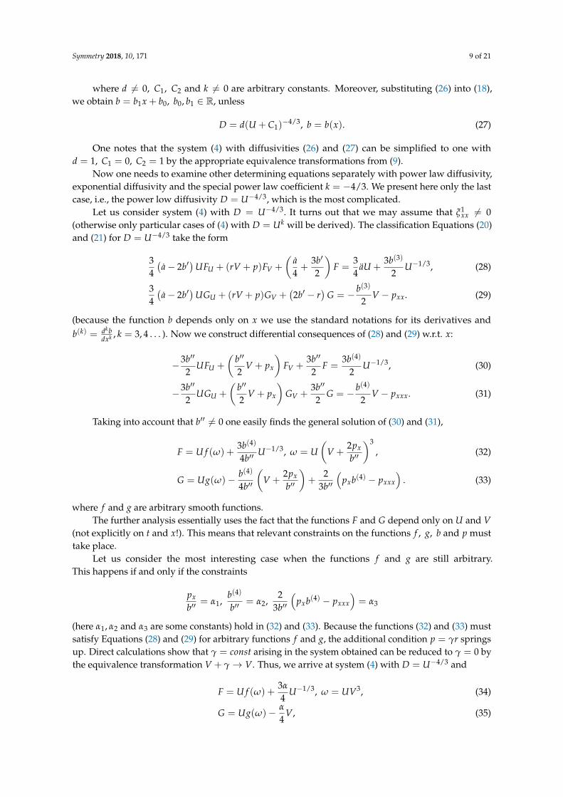
Now one needs to examine other determining equations separately with power law diffusivity,exponential diffusivity and the special power law coefficient k = −4/3. We present here only the lastcase, i.e., the power low diffusivity D = U−4/3, which is the most complicated.
Let us consider system (4) with D = U−4/3. It turns out that we may assume that ξ1xx 6= 0
(otherwise only particular cases of (4) with D = Uk will be derived). The classification Equations (20)and (21) for D = U−4/3 take the form
34(a− 2b′
)UFU + (rV + p)FV +
(a4+
3b′
2
)F =
34
aU +3b(3)
2U−1/3, (28)
34(a− 2b′
)UGU + (rV + p)GV +
(2b′ − r
)G = − b(3)
2V − pxx. (29)
(because the function b depends only on x we use the standard notations for its derivatives andb(k) = dkb
dxk , k = 3, 4 . . . ). Now we construct differential consequences of (28) and (29) w.r.t. x:
−3b′′
2UFU +
(b′′
2V + px
)FV +
3b′′
2F =
3b(4)
2U−1/3, (30)
−3b′′
2UGU +
(b′′
2V + px
)GV +
3b′′
2G = − b(4)
2V − pxxx. (31)
Taking into account that b′′ 6= 0 one easily finds the general solution of (30) and (31),
F = U f (ω) +3b(4)
4b′′U−1/3, ω = U
(V +
2px
b′′
)3, (32)
G = Ug(ω)− b(4)
4b′′
(V +
2px
b′′
)+
23b′′
(pxb(4) − pxxx
). (33)
where f and g are arbitrary smooth functions.The further analysis essentially uses the fact that the functions F and G depend only on U and V
(not explicitly on t and x!). This means that relevant constraints on the functions f , g, b and p musttake place.
Let us consider the most interesting case when the functions f and g are still arbitrary.This happens if and only if the constraints
px
b′′= α1,
b(4)
b′′= α2,
23b′′
(pxb(4) − pxxx
)= α3
(here α1, α2 and α3 are some constants) hold in (32) and (33). Because the functions (32) and (33) mustsatisfy Equations (28) and (29) for arbitrary functions f and g, the additional condition p = γr springsup. Direct calculations show that γ = const arising in the system obtained can be reduced to γ = 0 bythe equivalence transformation V + γ→ V. Thus, we arrive at system (4) with D = U−4/3 and
F = U f (ω) +3α
4U−1/3, ω = UV3, (34)
G = Ug(ω)− α
4V, (35)
Symmetry 2018, 10, 171 10 of 21
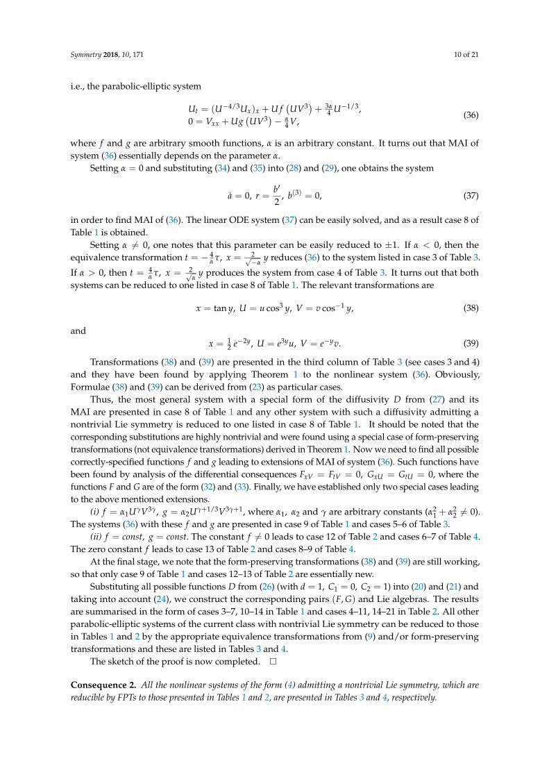
i.e., the parabolic-elliptic system
Ut = (U−4/3Ux)x + U f(UV3)+ 3α
4 U−1/3,0 = Vxx + Ug
(UV3)− α
4 V,(36)
where f and g are arbitrary smooth functions, α is an arbitrary constant. It turns out that MAI ofsystem (36) essentially depends on the parameter α.
Setting α = 0 and substituting (34) and (35) into (28) and (29), one obtains the system
a = 0, r =b′
2, b(3) = 0, (37)
in order to find MAI of (36). The linear ODE system (37) can be easily solved, and as a result case 8 ofTable 1 is obtained.
Setting α 6= 0, one notes that this parameter can be easily reduced to ±1. If α < 0, then theequivalence transformation t = − 4
α τ, x = 2√−α
y reduces (36) to the system listed in case 3 of Table 3.
If α > 0, then t = 4α τ, x = 2√
αy produces the system from case 4 of Table 3. It turns out that both
systems can be reduced to one listed in case 8 of Table 1. The relevant transformations are
x = tan y, U = u cos3 y, V = v cos−1 y, (38)
andx = 1
2 e−2y, U = e3yu, V = e−yv. (39)
Transformations (38) and (39) are presented in the third column of Table 3 (see cases 3 and 4)and they have been found by applying Theorem 1 to the nonlinear system (36). Obviously,Formulae (38) and (39) can be derived from (23) as particular cases.
Thus, the most general system with a special form of the diffusivity D from (27) and itsMAI are presented in case 8 of Table 1 and any other system with such a diffusivity admitting anontrivial Lie symmetry is reduced to one listed in case 8 of Table 1. It should be noted that thecorresponding substitutions are highly nontrivial and were found using a special case of form-preservingtransformations (not equivalence transformations) derived in Theorem 1. Now we need to find all possiblecorrectly-specified functions f and g leading to extensions of MAI of system (36). Such functions havebeen found by analysis of the differential consequences FxV = FtV = 0, GxU = GtU = 0, where thefunctions F and G are of the form (32) and (33). Finally, we have established only two special cases leadingto the above mentioned extensions.
(i) f = α1UγV3γ, g = α2Uγ+1/3V3γ+1, where α1, α2 and γ are arbitrary constants (α21 + α2
2 6= 0).The systems (36) with these f and g are presented in case 9 of Table 1 and cases 5–6 of Table 3.
(ii) f = const, g = const. The constant f 6= 0 leads to case 12 of Table 2 and cases 6–7 of Table 4.The zero constant f leads to case 13 of Table 2 and cases 8–9 of Table 4.
At the final stage, we note that the form-preserving transformations (38) and (39) are still working,so that only case 9 of Table 1 and cases 12–13 of Table 2 are essentially new.
Substituting all possible functions D from (26) (with d = 1, C1 = 0, C2 = 1) into (20) and (21) andtaking into account (24), we construct the corresponding pairs (F, G) and Lie algebras. The resultsare summarised in the form of cases 3–7, 10–14 in Table 1 and cases 4–11, 14–21 in Table 2. All otherparabolic-elliptic systems of the current class with nontrivial Lie symmetry can be reduced to thosein Tables 1 and 2 by the appropriate equivalence transformations from (9) and/or form-preservingtransformations and these are listed in Tables 3 and 4.
The sketch of the proof is now completed.
Consequence 2. All the nonlinear systems of the form (4) admitting a nontrivial Lie symmetry, which arereducible by FPTs to those presented in Tables 1 and 2, are presented in Tables 3 and 4, respectively.
Symmetry 2018, 10, 171 11 of 21
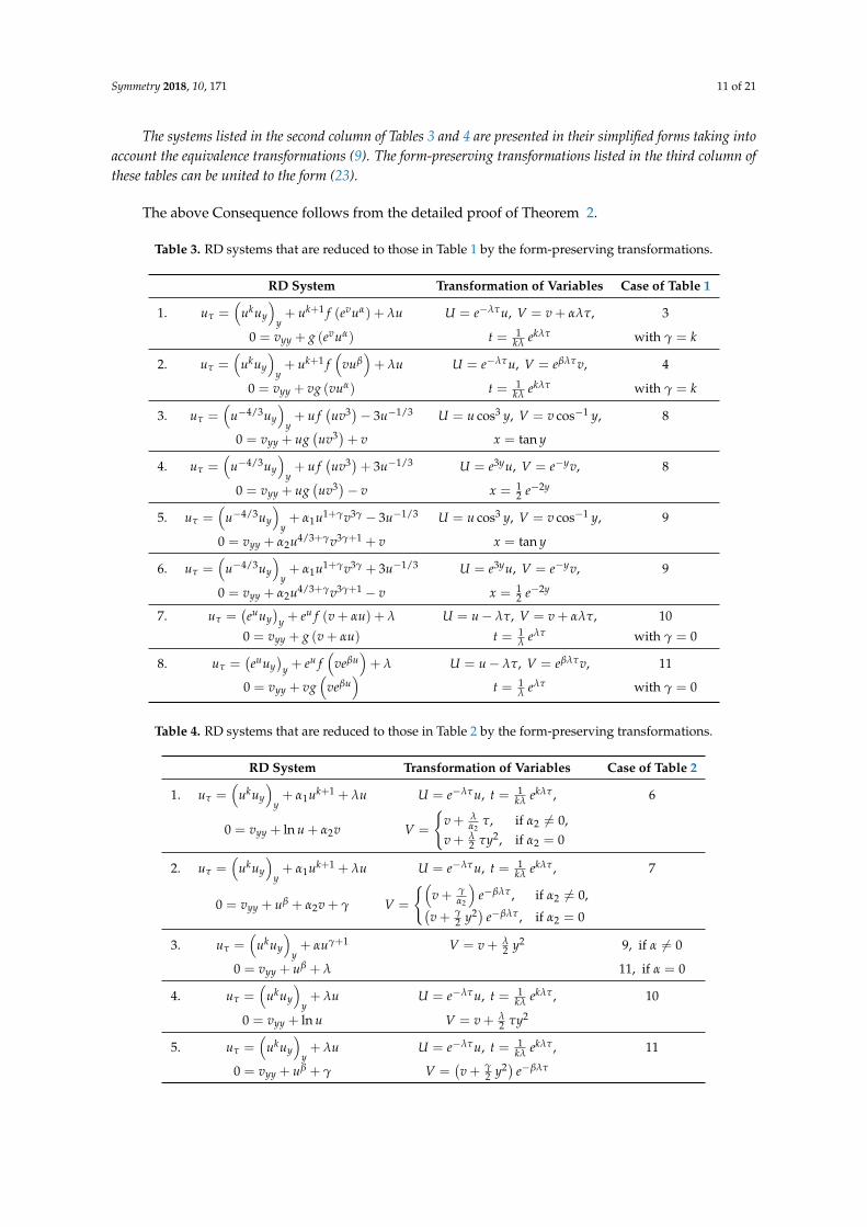
The systems listed in the second column of Tables 3 and 4 are presented in their simplified forms taking intoaccount the equivalence transformations (9). The form-preserving transformations listed in the third column ofthese tables can be united to the form (23).
The above Consequence follows from the detailed proof of Theorem 2.
Table 3. RD systems that are reduced to those in Table 1 by the form-preserving transformations.
RD System Transformation of Variables Case of Table 1
1. uτ =(
ukuy
)y+ uk+1 f (evuα) + λu U = e−λτu, V = v + αλτ, 3
0 = vyy + g (evuα) t = 1kλ ekλτ with γ = k
2. uτ =(
ukuy
)y+ uk+1 f
(vuβ
)+ λu U = e−λτu, V = eβλτv, 4
0 = vyy + vg (vuα) t = 1kλ ekλτ with γ = k
3. uτ =(
u−4/3uy
)y+ u f
(uv3)− 3u−1/3 U = u cos3 y, V = v cos−1 y, 8
0 = vyy + ug(uv3)+ v x = tan y
4. uτ =(
u−4/3uy
)y+ u f
(uv3)+ 3u−1/3 U = e3yu, V = e−yv, 8
0 = vyy + ug(uv3)− v x = 1
2 e−2y
5. uτ =(
u−4/3uy
)y+ α1u1+γv3γ − 3u−1/3 U = u cos3 y, V = v cos−1 y, 9
0 = vyy + α2u4/3+γv3γ+1 + v x = tan y
6. uτ =(
u−4/3uy
)y+ α1u1+γv3γ + 3u−1/3 U = e3yu, V = e−yv, 9
0 = vyy + α2u4/3+γv3γ+1 − v x = 12 e−2y
7. uτ =(euuy
)y + eu f (v + αu) + λ U = u− λτ, V = v + αλτ, 10
0 = vyy + g (v + αu) t = 1λ eλτ with γ = 0
8. uτ =(euuy
)y + eu f
(veβu
)+ λ U = u− λτ, V = eβλτv, 11
0 = vyy + vg(
veβu)
t = 1λ eλτ with γ = 0
Table 4. RD systems that are reduced to those in Table 2 by the form-preserving transformations.
RD System Transformation of Variables Case of Table 2
1. uτ =(
ukuy
)y+ α1uk+1 + λu U = e−λτu, t = 1
kλ ekλτ , 6
0 = vyy + ln u + α2v V =
{v + λ
α2τ, if α2 6= 0,
v + λ2 τy2, if α2 = 0
2. uτ =(
ukuy
)y+ α1uk+1 + λu U = e−λτu, t = 1
kλ ekλτ , 7
0 = vyy + uβ + α2v + γ V =
{(v + γ
α2
)e−βλτ , if α2 6= 0,(
v + γ2 y2) e−βλτ , if α2 = 0
3. uτ =(
ukuy
)y+ αuγ+1 V = v + λ
2 y2 9, if α 6= 0
0 = vyy + uβ + λ 11, if α = 0
4. uτ =(
ukuy
)y+ λu U = e−λτu, t = 1
kλ ekλτ , 10
0 = vyy + ln u V = v + λ2 τy2
5. uτ =(
ukuy
)y+ λu U = e−λτu, t = 1
kλ ekλτ , 11
0 = vyy + uβ + γ V =(v + γ
2 y2) e−βλτ
Symmetry 2018, 10, 171 12 of 21
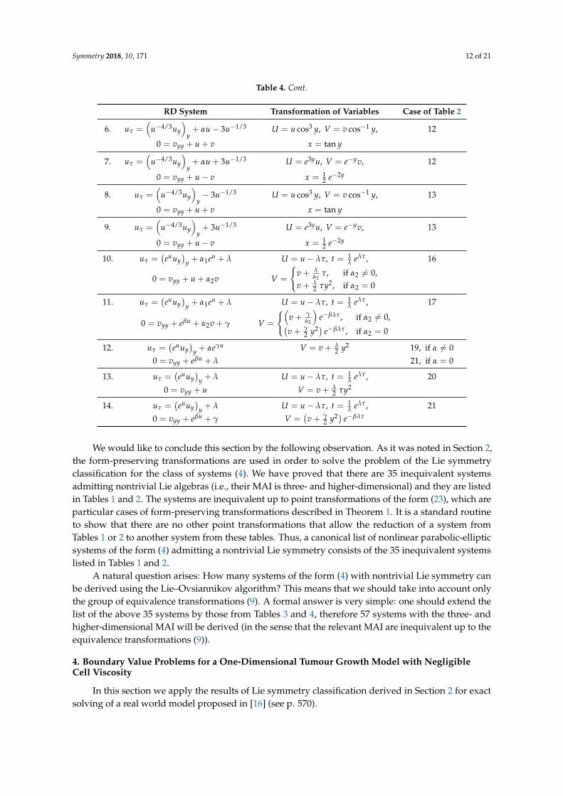
Table 4. Cont.
RD System Transformation of Variables Case of Table 2
6. uτ =(
u−4/3uy
)y+ αu− 3u−1/3 U = u cos3 y, V = v cos−1 y, 12
0 = vyy + u + v x = tan y
7. uτ =(
u−4/3uy
)y+ αu + 3u−1/3 U = e3yu, V = e−yv, 12
0 = vyy + u− v x = 12 e−2y
8. uτ =(
u−4/3uy
)y− 3u−1/3 U = u cos3 y, V = v cos−1 y, 13
0 = vyy + u + v x = tan y
9. uτ =(
u−4/3uy
)y+ 3u−1/3 U = e3yu, V = e−yv, 13
0 = vyy + u− v x = 12 e−2y
10. uτ =(euuy
)y + α1eu + λ U = u− λτ, t = 1
λ eλτ , 16
0 = vyy + u + α2v V =
{v + λ
α2τ, if α2 6= 0,
v + λ2 τy2, if α2 = 0
11. uτ =(euuy
)y + α1eu + λ U = u− λτ, t = 1
λ eλτ , 17
0 = vyy + eβu + α2v + γ V =
{(v + γ
α2
)e−βλτ , if α2 6= 0,(
v + γ2 y2) e−βλτ , if α2 = 0
12. uτ =(euuy
)y + αeγu V = v + λ
2 y2 19, if α 6= 0
0 = vyy + eβu + λ 21, if α = 0
13. uτ =(euuy
)y + λ U = u− λτ, t = 1
λ eλτ , 20
0 = vyy + u V = v + λ2 τy2
14. uτ =(euuy
)y + λ U = u− λτ, t = 1
λ eλτ , 21
0 = vyy + eβu + γ V =(v + γ
2 y2) e−βλτ
We would like to conclude this section by the following observation. As it was noted in Section 2,the form-preserving transformations are used in order to solve the problem of the Lie symmetryclassification for the class of systems (4). We have proved that there are 35 inequivalent systemsadmitting nontrivial Lie algebras (i.e., their MAI is three- and higher-dimensional) and they are listedin Tables 1 and 2. The systems are inequivalent up to point transformations of the form (23), which areparticular cases of form-preserving transformations described in Theorem 1. It is a standard routineto show that there are no other point transformations that allow the reduction of a system fromTables 1 or 2 to another system from these tables. Thus, a canonical list of nonlinear parabolic-ellipticsystems of the form (4) admitting a nontrivial Lie symmetry consists of the 35 inequivalent systemslisted in Tables 1 and 2.
A natural question arises: How many systems of the form (4) with nontrivial Lie symmetry canbe derived using the Lie–Ovsiannikov algorithm? This means that we should take into account onlythe group of equivalence transformations (9). A formal answer is very simple: one should extend thelist of the above 35 systems by those from Tables 3 and 4, therefore 57 systems with the three- andhigher-dimensional MAI will be derived (in the sense that the relevant MAI are inequivalent up to theequivalence transformations (9)).
4. Boundary Value Problems for a One-Dimensional Tumour Growth Model with NegligibleCell Viscosity
In this section we apply the results of Lie symmetry classification derived in Section 2 for exactsolving of a real world model proposed in [16] (see p. 570).
Symmetry 2018, 10, 171 13 of 21
Consider the pressure difference with r = 1 [16] (see p. 569 therein)
Σ(α) = k0α− α∗(1− α)q
assuming α > α∗. Setting
k(α) = k0α1−m(1− α)2 d(αΣ)dα
the equation (see (23) in [16]) for the tumour cell concentration, α(t, x), takes the form
αt = (αmαx)x + S(α, c). (40)
In order to simplify the boundary conditions we set
U = α− α∗, V = c∞ − c (41)
(wherein c corresponds to the level of nutrient in [16], but might instead correspond to that of achemotherapeutic drug) and arrive at the BVP
Ut = ((U + α∗)mUx)x + S(U + α∗, c∞ −V),0 = Vxx + Q(U + α∗, c∞ −V),x = 0 : Ux = Vx = 0,x = R(t) : U = V = 0,x = R(t) : R = −αm−1
∗ Ux,
(42)
where the concentrations U(t, x) and V(t, x) and the moving boundary location R(t) are unknownfunctions, while the functions S and Q are given smooth functions, and m, α∗ and c∞ arenonnegative parameters.
One may note that the governing equations of this BVP with S = f (U)V−β and Q = g(U)V−β+1
are a particular case of case 2 in Table 1, so that they admit the Lie symmetry operator
X = 2βt∂t + βx∂x + 2V∂V . (43)
It turns out that the following statement can be easily proved, using the definition of invariancefor BVPs with moving boundaries [32].
Theorem 3. The nonlinear BVP (42) with S = f (U)V−β and Q = g(U)V−β+1 is invariant with respect tothe two-dimensional MAI generated by the Lie symmetry operators (43) and ∂t.
Clearly the time translation operator ∂t cannot help to find any realistic solutions of BVP (42),while the Lie symmetry (43) guarantees a reduction of the problem, which leads to some interestingresults. In fact, the operator generates the ansatz
U = ϕ(ω), ω = x√t
,
V = t1β ψ(ω),
(44)
which immediately specifies the function R(t) = ω0√
t with the constant ω0 > 0 to be found.The reduced ODE problem is
(ϕ + α∗)m ϕ′′ + m(ϕ + α∗)m−1 (ϕ′)2 + ω2 ϕ′ + f (ϕ)ψ−β = 0,
ψ′′ + g(ϕ)ψ−β+1 = 0,ω = 0 : ϕ′ = ψ′ = 0,
ω = ω0 : ϕ = ψ = 0, ϕ′ = − α1−m∗ ω0
2 .
(45)
Symmetry 2018, 10, 171 14 of 21
The nonlinear BVP (45) is still a complicated problem and we were unable to solve it analyticallyin general. Let us consider a special case, namely (45) with β = 1 :
(ϕ + α∗)m ϕ′′ + m(ϕ + α∗)m−1 (ϕ′)2 + ω2 ϕ′ + f (ϕ)ψ−1 = 0,
ψ′′ + g(ϕ) = 0,ω = 0 : ϕ′ = ψ′ = 0,
ω = ω0 : ϕ = ψ = 0, ϕ′ = α1−m∗ ω0
2 .
(46)
In this case the exact solution can be found for arbitrary m in the form
ϕ = α1−m∗4(ω2
0 −ω2) , ω < ω0,
ψ = α1−m∗ q0
48(ω2
0 −ω2) (5ω20 −ω2) , ω < ω0
(47)
provided the functions f (ϕ) and g(ϕ) have the form
g = q0 ϕ, q0 > 0,
f = q0αm−1∗3 ϕ
(ϕ + α1−m
∗ ω20)
×((m + 1
2 )α1−m∗ (ϕ + α∗)m − mα2−m
∗4
(α−m∗ ω2
0 + 4)(ϕ + α∗)m−1 − ϕ + α1−m
∗4 ω2
0
).
(48)
Remark 3. A similar result can be obtained for arbitrary diffusivity in the governing equation (40), i.e., the dragcoefficient k(α), however, the structure of the function f (ϕ) will essentially depend on the diffusivity.
Now we present the final formulae for the original concentrations of tumour cells α(t, x) andnutrient (or drug) c(t, x) using Formulae (41), ansatz (44) and solution (47):
α(t, x) = α∗ +α1−m∗4
(ω2
0 −x2
t
), x < ω0
√t,
c(t, x) = c∞ − α1−m∗ q0
48 t(
ω20 −
x2
t
) (5ω2
0 −x2
t
), x < ω0
√t,
R(t) = ω0√
t.
(49)
Formulae (47) give the exact solution of the nonlinear BVP with a moving boundary for thegoverning equations
αt = (αmαx)x +f (α−α∗)
c−c∞,
0 = cxx − q0(α− α∗),(50)
and the boundary conditionsx = 0 : αx = cx = 0,x = R(t) : α = α∗, c = c∞,x = R(t) : R = − αx
α1−m∗
,(51)
where the function f is defined by (48), in particular one obtains the cubic polynomial for m = 0:
f =q0
3α∗(α− α∗)(α− α1)(α2 − α), α1 = α∗(1−ω2
0), α2 = α∗6 + ω2
04
, (52)
hence
S(α, c) =q0
3α∗
(α− α∗)(α− α1)(α2 − α)
c∞ − c. (53)
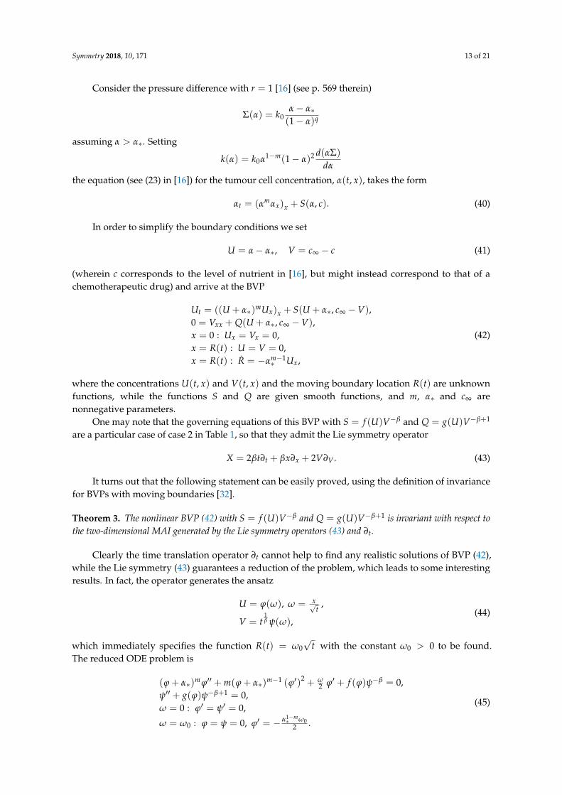
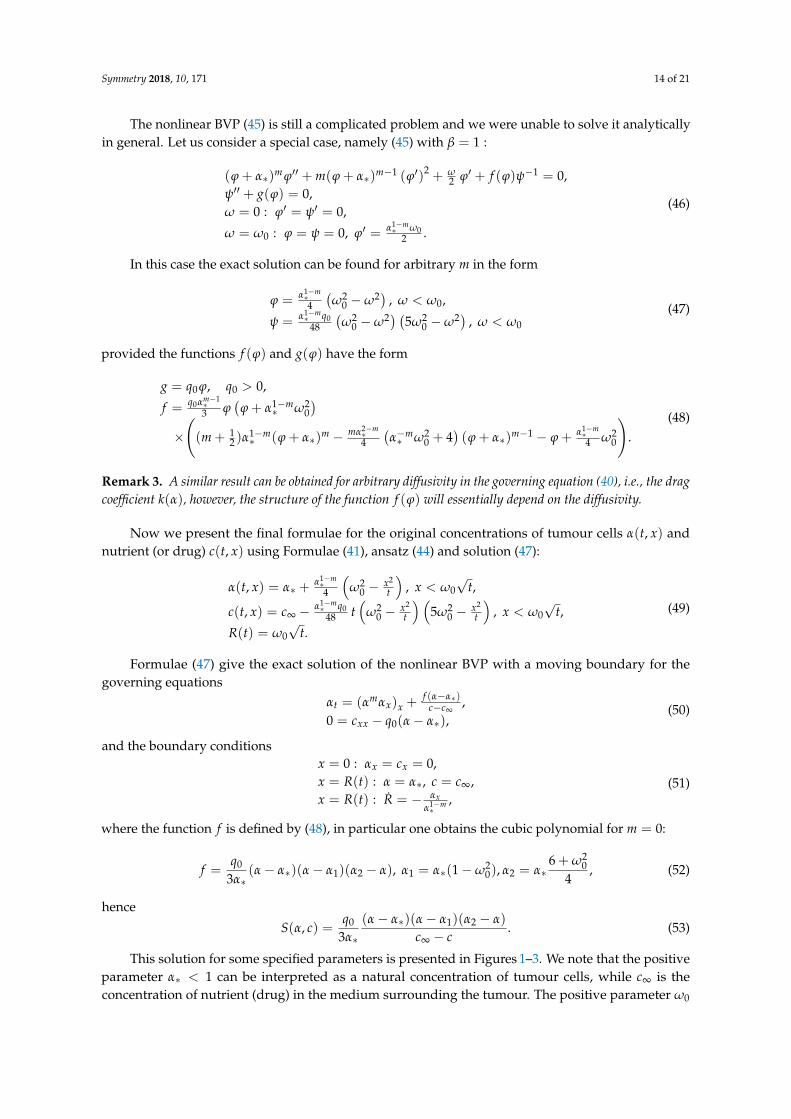
This solution for some specified parameters is presented in Figures 1–3. We note that the positiveparameter α∗ < 1 can be interpreted as a natural concentration of tumour cells, while c∞ is theconcentration of nutrient (drug) in the medium surrounding the tumour. The positive parameter ω0
Symmetry 2018, 10, 171 15 of 21
may be found from additional biologically motivated conditions. Notably the exact solution (49) canbe easily generalised to one with two arbitrary parameters by the time translation t→ t + t0.
Figure 1. Surfaces representing the concentrations α (left) and c (right) of the form (49) for theparameter values m = 1, α∗ = 0.5, c∞ = 2, ω0 = 1, q0 = 0.5.
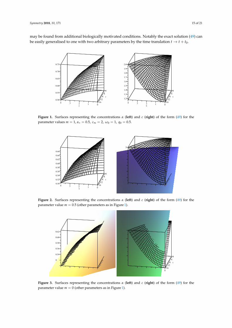
Figure 2. Surfaces representing the concentrations α (left) and c (right) of the form (49) for theparameter value m = 0.5 (other parameters as in Figure 1).
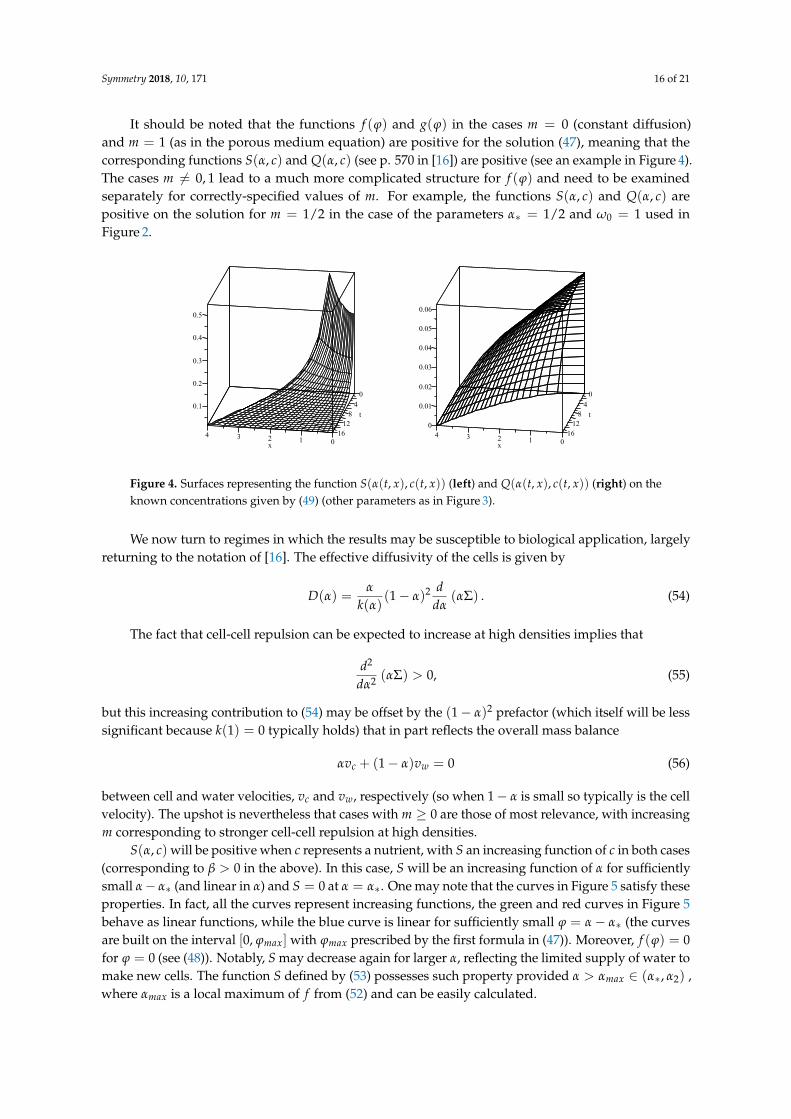
Figure 3. Surfaces representing the concentrations α (left) and c (right) of the form (49) for theparameter value m = 0 (other parameters as in Figure 1).
Symmetry 2018, 10, 171 16 of 21
It should be noted that the functions f (ϕ) and g(ϕ) in the cases m = 0 (constant diffusion)and m = 1 (as in the porous medium equation) are positive for the solution (47), meaning that thecorresponding functions S(α, c) and Q(α, c) (see p. 570 in [16]) are positive (see an example in Figure 4).The cases m 6= 0, 1 lead to a much more complicated structure for f (ϕ) and need to be examinedseparately for correctly-specified values of m. For example, the functions S(α, c) and Q(α, c) arepositive on the solution for m = 1/2 in the case of the parameters α∗ = 1/2 and ω0 = 1 used inFigure 2.
Figure 4. Surfaces representing the function S(α(t, x), c(t, x)) (left) and Q(α(t, x), c(t, x)) (right) on theknown concentrations given by (49) (other parameters as in Figure 3).
We now turn to regimes in which the results may be susceptible to biological application, largelyreturning to the notation of [16]. The effective diffusivity of the cells is given by
D(α) =α
k(α)(1− α)2 d
dα(αΣ) . (54)
The fact that cell-cell repulsion can be expected to increase at high densities implies that
d2
dα2 (αΣ) > 0, (55)
but this increasing contribution to (54) may be offset by the (1− α)2 prefactor (which itself will be lesssignificant because k(1) = 0 typically holds) that in part reflects the overall mass balance
αvc + (1− α)vw = 0 (56)
between cell and water velocities, vc and vw, respectively (so when 1− α is small so typically is the cellvelocity). The upshot is nevertheless that cases with m ≥ 0 are those of most relevance, with increasingm corresponding to stronger cell-cell repulsion at high densities.
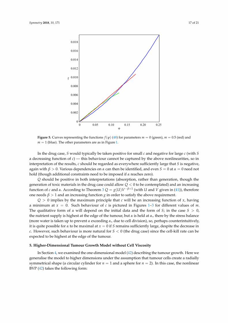
S(α, c) will be positive when c represents a nutrient, with S an increasing function of c in both cases(corresponding to β > 0 in the above). In this case, S will be an increasing function of α for sufficientlysmall α− α∗ (and linear in α) and S = 0 at α = α∗. One may note that the curves in Figure 5 satisfy theseproperties. In fact, all the curves represent increasing functions, the green and red curves in Figure 5behave as linear functions, while the blue curve is linear for sufficiently small ϕ = α− α∗ (the curvesare built on the interval [0, ϕmax] with ϕmax prescribed by the first formula in (47)). Moreover, f (ϕ) = 0for ϕ = 0 (see (48)). Notably, S may decrease again for larger α, reflecting the limited supply of water tomake new cells. The function S defined by (53) possesses such property provided α > αmax ∈ (α∗, α2) ,where αmax is a local maximum of f from (52) and can be easily calculated.
Symmetry 2018, 10, 171 17 of 21
Figure 5. Curves representing the functions f (ϕ) (48) for parameters m = 0 (green), m = 0.5 (red) andm = 1 (blue). The other parameters are as in Figure 1.
In the drug case, S would typically be taken positive for small c and negative for large c (with Sa decreasing function of c) — this behaviour cannot be captured by the above nonlinearities, so ininterpretation of the results, c should be regarded as everywhere sufficiently large that S is negative,again with β > 0. Various dependencies on α can then be identified, and even S = 0 at α = 0 need nothold (though additional constraints need to be imposed if α reaches zero).
Q should be positive in both interpretations (absorption, rather than generation, though thegeneration of toxic materials in the drug case could allow Q < 0 to be contemplated) and an increasingfunction of c and α. According to Theorem 3 Q = g(U)V−β+1 (with U and V given in (41)), thereforeone needs β > 1 and an increasing function g in order to satisfy the above requirement.
Q > 0 implies by the maximum principle that c will be an increasing function of x, havinga minimum at x = 0. Such behaviour of c is pictured in Figures 1–3 for different values of m.The qualitative form of α will depend on the initial data and the form of S; in the case S > 0,the nutrient supply is highest at the edge of the tumour, but α is held at α∗ there by the stress balance(more water is taken up to prevent α exceeding α∗ due to cell division), so, perhaps counterintuitively,it is quite possible for α to be maximal at x = 0 if S remains sufficiently large, despite the decrease inc. However, such behaviour is more natural for S < 0 (the drug case) since the cell-kill rate can beexpected to be highest at the edge of the tumour.
5. Higher-Dimensional Tumour Growth Model without Cell Viscosity
In Section 4, we examined the one-dimensional model (42) describing the tumour growth. Here wegeneralise the model to higher dimensions under the assumption that tumour cells create a radiallysymmetrical shape (a circular cylinder for n = 1 and a sphere for n = 2). In this case, the nonlinearBVP (42) takes the following form:
Symmetry 2018, 10, 171 18 of 21
Ut =1rn (rn(U + α∗)mUr)r + S(U + α∗, c∞ −V),
0 = 1rn (rnVr)r + Q(U + α∗, c∞ −V),
r = 0 : Ur = Vr = 0,r = R(t) : U = V = 0,r = R(t) : R = −αm−1
∗ Ur,
(57)
where n = 1, 2 and the same notations are used as in Section 4, however, the space variable x is
replaced by the variable r =√
x21 + · · ·+ x2
n + x2n+1.
One may check that the governing equations of this BVP with S = f (U)V−β and Q = g(U)V−β+1
are invariant w.r.t. the Lie symmetry operator
X = 2βt∂t + βr∂r + 2V∂V , (58)
which has the same structure as (43).
Theorem 4. The nonlinear BVP (57) with S = f (U)V−β and Q = g(U)V−β+1 is invariant with respect tothe two-dimensional MAI generated by the Lie symmetry operators (58) and ∂t.
Thus, the Lie symmetry (58) generates the ansatz
U = ϕ(ω), ω = r√t
,
V = t1β ψ(ω),
(59)
which immediately specifies the function R(t) = ω0√
t and reduces the two-dimensional BVP (57)(with S = f (U)V−β and Q = g(U)V−β+1) to the one-dimensional problem
(ϕ + α∗)m ϕ′′ + m(ϕ + α∗)m−1 (ϕ′)2 + nω (ϕ + α∗)m ϕ′ + ω
2 ϕ′ + f (ϕ)ψ−β = 0,ψ′′ + n
ω ψ′ + g(ϕ)ψ−β+1 = 0,ω = 0 : ϕ′ = ψ′ = 0,
ω = ω0 : ϕ = ψ = 0, ϕ′ = − α1−m∗ ω0
2 .
(60)
The nonlinear problem (60) is still not integrable for arbitrary given coefficients, however, one withβ = −1 is again a solvable case. Direct calculations show that Formulae (47) and (48) can be generalisedin this case as follows
ϕ = α1−m∗4(ω2
0 −ω2) , ω < ω0,
ψ = α1−m∗ q0
16(n+3)
(ω2
0 −ω2) ( n+5n+1 ω2
0 −ω2) , ω < ω0(61)
and
g = q0 ϕ, q0 > 0,
f = q0αm−1∗
n+3 ϕ
(ϕ +
α1−m∗ ω2
0n+1
)×((m + n+1
2 )α1−m∗ (ϕ + α∗)m − mα2−m
∗4
(α−m∗ ω2
0 + 4)(ϕ + α∗)m−1 − ϕ + α1−m
∗4 ω2
0
).
(62)
In order to obtain the final formulae for the original concentrations of tumour cells α(t, x) andnutrient (drug) c(t, x), we use Formulae (41), ansatz (59) and solution (61). The formulae obtainedcoincide with those presented in (49) for α(t, x) and R(t) while for the nutrient (drug) concentrationwe have the solution
Symmetry 2018, 10, 171 19 of 21
c(t, r) = c∞ −α1−m∗ q0
16(n + 3)t(
ω20 −
r2
t
)(n + 5n + 1
ω20 −
r2
t
), r < ω0
√t. (63)
The biomedical interpretation of the various regimes coincides with that in Section 4 and isomitted here.
6. Conclusions
The main part of this paper is devoted to the Lie symmetry classification of the class ofparabolic-elliptic systems (3). First of all, the structure of form-preserving (admissible) transformationsfor the systems of the form (3) is established (see Theorem 1) in order to establish possible relationsbetween systems that admit equivalent MAIs. Theorem 2 gives a complete list of inequivalentparabolic-elliptic systems consisting of 35 systems, which are invariant under nontrivial MAIs,i.e., under the three- and higher-dimensional Lie algebras. Moreover, we have established all possiblesubclasses of parabolic-elliptic systems (see Tables 3 and 4) with nontrivial Lie symmetry, which arereducible to those listed in Tables 1 and 2 by the relevant form-preserving transformations. Notably,our result is a new confirmation of importance of finding form-preserving transformations becausethey allow reducing essentially (in contrast to the group of equivalence transformations) the number ofinequivalent systems. In fact, the traditional Lie–Ovsiannikov algorithm, which is based on the groupof equivalence transformations, would lead to 57 parabolic-elliptic systems instead of 35 systems listedin Tables 1 and 2 because 22 systems from Tables 3 and 4 should be added.
From the applicability point of view, the most interesting parabolic-elliptic systems occur inTable 1 because the systems from Table 2 are semi-coupled. It is worth noting that MAIs for the systemsarising in all the cases of Table 1 excepting 7 and 14 are some analogs of those for single RD equations.In fact, fixing the diffusion coefficient in the first equation of the corresponding system one may easilyidentify its generic analog in Table 4 [24] (see cases 3–5 and 7 therein). For example, MAIs of thesystems from cases 8 and 9 contain the well-known algebra sl(2,R) as a subalgebra (see the second,third and fourth operators in the last column). The same subalgebra occurs for the diffusion equationwith the same diffusivity (see case 3 in Table 4 [24]). By the way, Ovsiannikov was the first to identifythis special case for nonlinear diffusion equations [17]. Of course, the systems in Table 1 have moregeneral structures (many of them contain arbitrary functions as coefficients) in contrast to their analogslisted in Table 4 [24]. However, it happens on a regular basis if one considers systems instead of singleequations (see, e.g., case 10 in Table 1 [13] involving the same diffusivity).
Cases 7 and 14 in Table 1 have no analogs among single RD equations. Moreover, the relevantMAIs generate infinite-dimensional Lie algebras because they contain the operators X∞ involving anarbitrary smooth function ϕ(t) (see the last column of Table 1). Interestingly, both MAIs from Cases7 and 14 again contain the well-known algebra sl(2,R) as a subalgebra. In fact, if one sets ϕ(t) = tand ϕ(t) = t2 then the operators ∂t, X∞ with ϕ(t) = t and X∞ with ϕ(t) = t2 produce nothing elsebut sl(2,R) with new representations (it is a simple task to check the commutator relations), which donot happen in the case of single RD equations.
In order to demonstrate applicability of our pure theoretical result, we apply the Lie symmetrycorresponding to one-parameter group of scale transformation for solving a (1+1)-dimensional BVPwith a free boundary modeling tumour growth [16]. We reduce the given nonlinear BVP to thatgoverned by ODEs. As a result, its exact solution was constructed under additional restrictions onthe coefficients arising in the governing equations. Moreover, possible biological interpretationsof the solution are discussed. In particular, it was shown that the results obtained allow plausibleinterpretation in the case when the model describes growth of tumour cells consuming a nutrient.Finally, the results for the above (1+1)-dimensional BVP were generalised on multi-dimensional caseunder the assumption that tumour cells create a radially symmetrical shape. In a forthcoming paper,we will generalise these results using the definition of conditional invariance for BVPs introducedin [33].

Symmetry 2018, 10, 171 20 of 21
Author Contributions: All the authors contributed equally to the work. All authors read and approved thefinal manuscript.
Acknowledgments: This research was supported by a Marie Curie International Incoming Fellowship to the firstauthor within the 7th European Community Framework Programme (project BVPsymmetry 912563).
Conflicts of Interest: The authors declare no conflict of interest.
References
1. Ames, W.F. Nonlinear Partial Differential Equations in Engineering; Academic: New York, NY, USA, 1972;ISBN 9780080955247.
2. Murray, J.D. Mathematical Biology; Springer: Berlin, Germany, 1989.3. Murray, J.D. Mathematical Biology, II: Spatial Models and Biomedical Applications; Springer: Berlin, Germany, 2003.4. Okubo, A.; Levin, S.A. Diffusion and Ecological Problems. Modern Perspectives, 2nd ed.; Springer: Berlin,
Germany, 2001.5. Lotka, A.J. Undamped oscillations derived from the law of mass action. J. Am. Chem. Soc. 1920, 42, 1595–1599,
doi:10.1021/ja01453a010. [CrossRef]6. Volterra, V. Variazionie fluttuazioni del numero d‘individui in specie animali conviventi. Mem. Acad. Lincei
1926, 2, 31–113. (In Italian)7. Turing, A.M. The chemical basis of morphogenesis. Philos. Trans. R. Soc. B 1952, 237, 37–72. [CrossRef]8. Zulehner, W.; Ames, W.F. Group analysis of a semilinear vector diffusion equation. Nonlinear Anal. 1983, 7,
945–969. [CrossRef]9. Cherniha, R.; King, J.R. Lie symmetries of nonlinear multidimensional reaction-diffusion systems: I. J. Phys.
A Math. Gen. 2000, 33, 267–282. [CrossRef]10. Cherniha, R.; King, J.R. Addendum: Lie symmetries of nonlinear multidimensional reaction-dfiffusion
systems: I. J. Phys. A Math. Gen. 2000, 33, 7839–7841. [CrossRef]11. Cherniha, R.; King, J.R. Lie symmetries of nonlinear multidimensional reaction-diffusion systems: II. J. Phys.
A Math. Gen. 2003, 36, 405–425. [CrossRef]12. Knyazeva, I.V.; Popov, M.D. A system of two diffusion equations. In CRC Handbook of Lie Group Analysis of
Differential Equations; CRC Press: Boca Raton, FL, USA, 1994; Volume 1, pp. 171–176.13. Cherniha, R.; King, J.R. Non-linear reaction-diffusion systems with variable diffusivities: Lie symmetries,
ansatze and exact solutions. J. Math. Anal. Appl. 2005, 308, 11–35. [CrossRef]14. Cherniha, R.; King, J.R. Lie symmetries and conservation laws of non-linear multidimensional
reaction–diffusion systems with variable diffusivities. IMA J. Appl. Math. 2006, 71, 391–408. [CrossRef]15. Torrisi, M.; Tracina, R. An application of equivalence transformations to reaction diffusion equations.
Symmetry 2015, 7, 1929–1944. [CrossRef]16. Byrne, H.; King, J.R.; McElwain, D.L.S.; Preziosi, L. A two-phase model of solid tumour growth.
Appl. Math. Lett. 2003, 16, 567–573, doi:10.1016/S0893-9659(03)00038-7. [CrossRef]17. Ovsiannikov, L.V. Group relations of the equation of non-linear heat conductivity. Dokl. Akad. Nauk SSSR
1959, 125, 492–495. (In Russian)18. Kingston, J.G. On point transformations of evolution equations. J. Phys. A Math. Gen. 1991, 24, L769–L774,
doi:10.1088/0305-4470/24/14/003. [CrossRef]19. Kingston, J.G.; Sophocleous, C. On form-preserving point transformations of partial differential equations.
J. Phys. A Math. Gen. 1998, 31, 1597–1619. [CrossRef]20. Niederer, U. Schrödinger invariant generalised heat equation. Helv. Phys. Acta 1978, 51, 220–239.21. Gazeau, J.P.; Winternitz, P. Symmetries of variable coefficient Korteweg-de Vries equations. J. Math. Phys.
1992, 33, 4087–4102. [CrossRef]22. Ames, W.F.; Anderson, R.L.; Dorodnitsyn, V.A.; Ferapontov, E.V.; Gazizov, R.K.; Ibragimov, N.H.;
Svirshchevskiy, S.R. CRC Handbook of Lie Group Analysis of Differential Equations, vol. 1. Symmetries, ExactSolutions And Conservation Laws; CRC Press: Boca Raton, FL, USA, 1994; pp. 133–136.
23. Cherniha, R.; Serov, M. Symmetries, ansätze and exact solutions of nonlinear second-order evolutionequations with convection term. Eur. J. Appl. Math. 1998, 9, 527–542. [CrossRef]
24. Cherniha, R.; Serov, M.; Rassokha, I. Lie symmetries and form-preserving transformations ofreaction-diffusion-convection equations. J. Math. Anal. Appl. 2008, 342, 1363–1379. [CrossRef]
Symmetry 2018, 10, 171 21 of 21
25. Cherniha, R.; Serov, M.; Pliukhin, O. Nonlinear Reaction-Diffusion-Convection Equations: Lie and ConditionalSymmetry, Exact Solutions and Their Applications; CRC Press Taylor and Francis Group: Boka Raton, FL, USA,2018; ISBN 9781498776172.
26. Cherniha, R.; Davydovych, V. Reaction-diffusion systems with constant diffusivities: Conditionalsymmetries and form-preserving transformations. In Algebra, Geometry and Mathematical Physics; Springer:Berlin/Heidelberg, Germany, 2014; Volume 85, pp. 533–553.
27. Arrigo, D.J. Symmetry Analysis of Differential Equations: An Introduction; John Wiley and Sons: Hoboken, NJ,USA, 2015; ISBN 9781118721445.
28. Bluman, G.W.; Anco, S.C. Symmetry and Integration Methods for Differential Equations; Springer: New York,NY, USA, 2002; ISBN 9780387216492.
29. Bluman, G.W.; Kumei, S. Symmetries and Differential Equations; Springer: Berlin, Germany, 1989.30. Fushchych, W.I.; Shtelen, W.M.; Serov, M.I. Symmetry Analysis and Exact Solutions of Equations of Nonlinear
Mathematical Physics; Kluwer: Dordrecht, The Netherlands, 1993.31. Olver, P.J. Applications of Lie Groups to Differential Equations; Springer: Berlin, Germany, 1986;
ISBN 978-1-4684-0274-2.32. Cherniha, R.; Kovalenko, S. Lie symmetries and reductions of multi-dimensional boundary value problems
of the Stefan type. J. Phys. A Math. Theor. 2011, 44, 485202, doi:10.1088/1751-8113/44/48/485202 [CrossRef]33. Cherniha, R.; King, J.R. Lie and Conditional Symmetries of a Class of Nonlinear (1 + 2)—Dimensional
Boundary Value Problems. Symmetry 2015, 7, 1410–1435. [CrossRef]
c© 2018 by the authors. Licensee MDPI, Basel, Switzerland. This article is an open accessarticle distributed under the terms and conditions of the Creative Commons Attribution(CC BY) license (http://creativecommons.org/licenses/by/4.0/).