Embed Size (px)
Citation preview

Lie groups
Stefan Weinzierl
July 9, 2008
1

Contents1 Introduction 4
1.1 Content . . . . . . . . . . . . . . . . . . . . . . . . . . . . . . . . . . . . . . . 41.2 Literature . . . . . . . . . . . . . . . . . . . . . . . . . . . . . . . . . . . . . . 4
2 Basics 52.1 Groups . . . . . . . . . . . . . . . . . . . . . . . . . . . . . . . . . . . . . . . . 5
2.1.1 Definition . . . . . . . . . . . . . . . . . . . . . . . . . . . . . . . . . . 52.1.2 Examples . . . . . . . . . . . . . . . . . . . . . . . . . . . . . . . . . . 62.1.3 Morphisms . . . . . . . . . . . . . . . . . . . . . . . . . . . . . . . . . 8
2.2 Manifolds . . . . . . . . . . . . . . . . . . . . . . . . . . . . . . . . . . . . . . 82.2.1 Definition . . . . . . . . . . . . . . . . . . . . . . . . . . . . . . . . . . 82.2.2 Examples . . . . . . . . . . . . . . . . . . . . . . . . . . . . . . . . . . 92.2.3 Morphisms . . . . . . . . . . . . . . . . . . . . . . . . . . . . . . . . . 10
2.3 Lie groups . . . . . . . . . . . . . . . . . . . . . . . . . . . . . . . . . . . . . . 102.3.1 Definition . . . . . . . . . . . . . . . . . . . . . . . . . . . . . . . . . . 102.3.2 Examples . . . . . . . . . . . . . . . . . . . . . . . . . . . . . . . . . . 10
2.4 Algebras . . . . . . . . . . . . . . . . . . . . . . . . . . . . . . . . . . . . . . . 122.4.1 Definition . . . . . . . . . . . . . . . . . . . . . . . . . . . . . . . . . . 122.4.2 Examples . . . . . . . . . . . . . . . . . . . . . . . . . . . . . . . . . . 12
2.5 Lie algebras . . . . . . . . . . . . . . . . . . . . . . . . . . . . . . . . . . . . . 132.5.1 Definition . . . . . . . . . . . . . . . . . . . . . . . . . . . . . . . . . . 132.5.2 The exponential map . . . . . . . . . . . . . . . . . . . . . . . . . . . . 132.5.3 Relation between Lie algebras and Lie groups . . . . . . . . . . . . . . . 152.5.4 Examples . . . . . . . . . . . . . . . . . . . . . . . . . . . . . . . . . . 172.5.5 The Fierz identity . . . . . . . . . . . . . . . . . . . . . . . . . . . . . . 18
3 Representation theory 213.1 Group actions . . . . . . . . . . . . . . . . . . . . . . . . . . . . . . . . . . . . 213.2 Representations . . . . . . . . . . . . . . . . . . . . . . . . . . . . . . . . . . . 213.3 Schur’s lemmas . . . . . . . . . . . . . . . . . . . . . . . . . . . . . . . . . . . 233.4 Representation theory for finite groups . . . . . . . . . . . . . . . . . . . . . . . 26
3.4.1 Characters . . . . . . . . . . . . . . . . . . . . . . . . . . . . . . . . . 273.5 Representation theory for Lie groups . . . . . . . . . . . . . . . . . . . . . . . . 29
3.5.1 Irreducible representation of SU(2) and SO(3) . . . . . . . . . . . . . . 293.5.2 The Cartan basis . . . . . . . . . . . . . . . . . . . . . . . . . . . . . . 323.5.3 Weights . . . . . . . . . . . . . . . . . . . . . . . . . . . . . . . . . . . 37
3.6 Tensor methods . . . . . . . . . . . . . . . . . . . . . . . . . . . . . . . . . . . 403.6.1 Clebsch-Gordan series . . . . . . . . . . . . . . . . . . . . . . . . . . . 403.6.2 The Wigner-Eckart theorem . . . . . . . . . . . . . . . . . . . . . . . . 423.6.3 Young diagrams . . . . . . . . . . . . . . . . . . . . . . . . . . . . . . 43
2

4 The classification of semi-simple Lie algebras 474.1 Dynkin diagrams . . . . . . . . . . . . . . . . . . . . . . . . . . . . . . . . . . 504.2 The classification . . . . . . . . . . . . . . . . . . . . . . . . . . . . . . . . . . 514.3 Proof of the classification . . . . . . . . . . . . . . . . . . . . . . . . . . . . . . 53
3

1 Introduction
1.1 Content- Basics
- Representation theory
- Classifikation of semi-simple groups
1.2 Literature• Introductory texts:
- W. Fulton and J. Harris, Representation theory, Springer, 1991
- B. Hall, Lie groups, Lie Algebras and Representations, Springer, 2003
• Physics related:
- M. Schottenloher, Geometrie und Symmetrie in der Physik, Vieweg, 1995
- M. Nakahara, Geometry, Topology and Physics, IOP, 1990
• Classics:
- N. Bourbaki, Groupes et algèbres de Lie, Hermann, 1972
- H. Weyl, The classical groups, Princeton University Press, 1946
• Differential geometry:
- S. Helgason, Differential Geometry, Lie Groups and Symmetric Spaces, AMS, 1978
• Hopf algebras:
- Ch. Kassel, Quantum Groups, Springer, 1995
• Specialised topics:
- Ch. Reutenauer, Free Lie Algebras, Clarendon Press, 1993
- V. Kac, Infinite dimensional Lie algebras, Cambridge University Press, 1983
4

2 Basics
2.1 Groups2.1.1 Definition
A non-empty set G together with a composition · : G×G → G is called a group (G, ·) if
G1: The composition · is associative : a · (b · c) = (a ·b) · c
G2: There exists a neutral element : e ·a = a · e = a for all a ∈ G
G3: For all a ∈ G there exists an inverse a−1 : a−1 ·a = a ·a−1 = e
One can actually use a weaker system of axioms:
G1’: The composition · is associative : a · (b · c) = (a ·b) · c
G2’: There exists a left-neutral element : e ·a = a for all a ∈ G
G3’: For all a ∈ G there exists an left-inverse a−1 : a−1 ·a = e
The first system of axioms clearly implies the second system of axioms. To show that the secondsystem also implies the first one, we show the following:a) If e is a left-neutral element, and e′ is a right-neutral element, then e = e′.Proof:
e′ = e · e′ e is left-neutral= e, e′ is right-neutral
b) If b is a left-inverse to a, and b′ is a right-inverse to a, then b = b′.Proof:
b = b · e e is right-neutral
= b ·(a ·b′
)b′ is right-inverse of a
= (b ·a) ·b′ associativity= e ·b′ b is left-inverse of a= b′ e is left-neutral
c) If b is a left-inverse to a, i.e. b ·a = e, then b is also the right-inverse to a.Proof:
(a ·b) · (a ·b) = a · (b ·a) ·b= a · e ·b= a ·b
5

Therefore a ·b = e.d) If e is the left-neutral element, then e is also right-neutral.Proof:
a = e ·a=(a−1 ·a
)·a
=(a ·a−1) ·a
= a ·(a−1 ·a
)
= a · e
This completes the proof that the second system of axioms is equivalent to the first system ofaxioms. To verify that a given set together with a given composition forms a group it is thereforesufficient to verify axioms (G2’) and (G3’) instead of axioms (G2) and (G3).
More definitions:A group (G, ·) is called Abelian if the operation · is commutative : a ·b = b ·a.
The number of elements in the set G is called the order of the group. If this number is finite,we speak of a finite group. In the case where the order is infinite, we can further distinguish thecase where the set is countable or not. For Lie groups we are in particular interested in the lattercase.
2.1.2 Examples
a) The trivial example: Let G = e and e · e = e. This is a group with one element.
b) Z2: Let G = 0,1 and denote the composition by +. The composition is given by thefollowing composition table:
+ 0 10 0 11 1 0
Z2 is of order 2 and is Abelian.
c) Zn: We can generalise the above example and take G = 0,1,2, ...,n− 1. We define theaddition by
a+b = a+b mod n,
where on the l.h.s. “+” denotes the composition in Zn, whereas on the r.h.s. “+” denotes theusual addition of integer numbers. Zn is a group of order n and is Abelian.
6
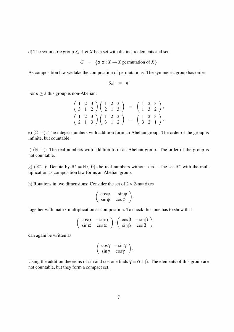
d) The symmetric group Sn: Let X be a set with distinct n elements and set
G = σ|σ : X → X permutation of X
As composition law we take the composition of permutations. The symmetric group has order
|Sn| = n!
For n ≥ 3 this group is non-Abelian:(
1 2 33 1 2
)(1 2 32 1 3
)
=
(1 2 31 3 2
)
,
(1 2 32 1 3
)(1 2 33 1 2
)
=
(1 2 33 2 1
)
.
e) (Z,+): The integer numbers with addition form an Abelian group. The order of the group isinfinite, but countable.
f) (R,+): The real numbers with addition form an Abelian group. The order of the group isnot countable.
g) (R∗, ·): Denote by R∗ = R\0 the real numbers without zero. The set R∗ with the mul-tiplication as composition law forms an Abelian group.
h) Rotations in two dimensions: Consider the set of 2×2-matrixes(
cosϕ −sinϕsinϕ cosϕ
)
,
together with matrix multiplication as composition. To check this, one has to show that(
cosα −sinαsinα cosα
)
·(
cosβ −sinβsinβ cosβ
)
can again be written as(
cosγ −sinγsinγ cosγ
)
.
Using the addition theorems of sin and cos one finds γ = α + β. The elements of this group arenot countable, but they form a compact set.
7

2.1.3 Morphisms
Let a and b be elements of a group (G,∗) with composition ∗ and let a′ and b′ be elements of agroup (G,) with composition . We are interested in mappings between groups which preservethe structure of the compositions.
Homomorphism: We call a mapping f : G → G′ a homomorphism, if
f (a∗b) = f (a) f (b).
Isomorphism: We call a mapping f : G → G′ an isomorphism, if it is bijective and a homomor-phism.
Automorphism: We call a mapping f : G → G from the group G into the group G itself anautomorphism, if it is an isomorphism.
2.2 Manifolds2.2.1 Definition
A topological space is a set M together with a family T of subsets of M satisfying the followingproperties:
1. /0 ∈ T , M ∈ T
2. U1,U2 ∈ T ⇒U1 ∩U2 ∈ T
3. For any index set A we have Uα ∈ T ;α ∈ A ⇒ S
α∈AUα ∈ T
The sets U ∈ T are called open.
A topological space is called Hausdorff if for any two distinct points p1, p2 ∈ M there existsopen sets U1,U2 ∈ T with
p1 ∈U1, p2 ∈U2, U1 ∩U2 = /0.
A map between topological spaces is called continous if the preimage of any open set is againopen.
A bijective map which is continous in both directions is called a homeomorphism.
An open chart on M is a pair (U,ϕ), where U is an open subset of M and ϕ is a homeomorphismof U onto an open subset of Rn.
A differentiable manifold of dimension n is a Hausdorff space with a collection of open charts(Uα,ϕα)α∈A such that
8
M1:
M =[
α∈A
Uα.
M2: For each pair α,β ∈ A the mapping ϕβ ϕ−1α is an infinitely differentiable mapping of
ϕα(Uα ∩Uβ
)onto ϕβ
(Uα∩Uβ
).
A differentiable manifold is also often denoted as a C∞ manifold. As we will only be concernedwith differentiable manifolds, we will often omitt the word “differentiable” and just speak aboutmanifolds.
The collection of open charts (Uα,ϕα)α∈A is called an atlas.
If p ∈Uα and
ϕα(p) = (x1(p), ...,xn(p)) ,
the set Uα is called the coordinate neighbourhood of p and the numbers xi(p) are called thelocal coordinates of p.
Note that in each coordinate neighbourhood M looks like an open subset of Rn. But note that wedo not require that M be Rn globally.
Consider two manifolds M and N with dimensions m and n. Let xi be coordinates on M andy j be coordinates on N. A mapping f : M → N between two manifolds is called analytic, if foreach point p ∈ M there exits a neighbourhood U of p and n power series Pj, j = 1, ...,n such that
y j( f (q)) = Pj (x1(q)− x1(p), ...,xm(q)− xm(p))
for all q ∈U .
An analytic manifold is a manifold where the mapping ϕβ ϕ−1α is analytic.
2.2.2 Examples
a) Rn: The space Rn is a manifold. Rn can be covered with a single chart.
b) S1: The circle
S1 = ~x ∈ R2||~x|2 = 1
is a manifold. For an atlas we need at least two charts.
c) The set of rotation matrices in two dimensions:(
cosϕ −sinϕsinϕ cosϕ
)
,
The set of all these matrices forms a manifold homeomorphic to the circle S1.
9

2.2.3 Morphisms
Homeomorphism: A map f : M → N between two manifolds M and N is called a homeo-morphism if it is bijective and both the mapping f : M → N and the inverse f −1 : N → M arecontinous.
Diffeomorphism: A map f : M → N is called a diffeomorphism if it is a homeomorphism andboth f and f−1 are infinitely differentiable.
Analytic diffeomorphism: The map f : M → N is a diffeomorphism and analytic.
2.3 Lie groups2.3.1 Definition
A Lie group G is a group which is also an analytic manifold, such that the mappings
G×G → G,
(a,b) → a ·b,
and
G → G,
a → a−1
are analytic.
Remark: Instead of the two mappings above, it is sufficient to require that the mapping
G×G → G,
(a,b) → a ·b−1
is analytic.
2.3.2 Examples
The most important examples of Lie groups are matrix groups with matrix multiplication as com-position. In order to have an inverse, the matrices must be non-singular.
a) GL(n,R), GL(n,C): The group of non-singular n× n matrices with real or complex entries.GL(n,R) has n2 real parameters, GL(n,C) has 2n2 real parameters.
b) SL(n,R), SL(n,C): The group of non-singular n× n matrices with real or complex entriesand
det A = 1.
10

SL(n,R) has n2 −1 real parameters, while SL(n,C) has 2(n2−1) real parameters.
c) O(n) : The group of orthogonal n×n matrices defined through
RRT = 1.
The group O(n) has n(n− 1)/2 real parameters. The group O(n) can also be defined as thetransformation group of a real n-dimensional vector space, which preserves the inner product
n
∑i=1
x2i
d) SO(n): The group of special orthogonal n×n matrices defined through
RRT = 1 and det R = 1.
The group SO(n) has n(n−1)/2 real parameters.
e) U(n): The group of unitary n×n matrices defined through
UU† = 1.
The group U(n) has n2 real parameters. The group U(n) can also be defined as the transformationgroup of a complex n-dimensional vector space, which preserves the inner product
n
∑i=1
z∗i zi
f) SU(n): The group of special unitary n×n matrices defined through
UU† = 1 and det U = 1.
The group SU(n) has n2 −1 real parameters.
g) Sp(n,R): The symplectic group is the group of 2n×2n matrices satisfying
MT(
0 In−In 0
)
M =
(0 In
−In 0
)
The group Sp(n,R) has (2n+1)n real parameters. The group Sp(n,R) can also be defined as thetransformation group of a real 2n-dimensional vector space, which preserves the inner product
n
∑j=1
(x jy j+n − x j+ny j
).
11

2.4 Algebras2.4.1 Definition
Let K be a field and A a vector space over the field K. A is called an algebra, if there is anadditional composition
A×A → A(a1,a2) → a1a2
such that the algebra multiplication is K-linear.
(r1a1 + r2a2)a3 = r1(a1a3)+ r2(a2a3)
a3(r1a1 + r2a2) = r1(a3a1)+ r2(a3a2)
Remark: It is not necessary to require that K is a field. It is sufficient to have a commutative ringR with 1. In this case one replaces the requirement for A to be a vector space by the requirementthat A is an unital R-modul. The difference between a field K and a commutative ring R with 1lies in the fact that in the ring R the multiplicative inverse might not exist.
An algebra is called associative if
(a1a2)a3 = a1(a2a3)
An algebra is called commutative if
a1a2 = a2a1
An unit element 1A ∈ A satisfies
1A a = a.
Note that it is not required that A has a unit element. If there is one, note that difference between1A ∈ A and 1K ∈ K: The latter always exists and we have the scalar multiplication with one:
1K a = a.
2.4.2 Examples
a) Consider the set of n×n matrices over R with the composition given by matrix multiplication.This gives an associative, non-commutative algebra with a unit element given by the unit matrix.
b) Consider the set of n×n matrices over R where the composition is defined by
[a,b] = ab−ba.
This defines a non-associative, non-commutative algebra. There is no unit element.
12
2.5 Lie algebras2.5.1 Definition
For a Lie algebra it is common practice to denote the composition of two elements a and b by[a,b]. An algebra is called a Lie-algebra if the composition satisfies
[a,a] = 0,
[a, [b,c]]+ [b, [c,a]]+ [c, [a,b]] = 0.
Remark: Consider again the example above of the set of n× n matrices over R where the com-position is defined by the commutator
[a,b] = ab−ba.
Clearly this definition satisfies [a,a] = 0. It fullfills the Jacobi identity:
[a, [b,c]]+ [b, [c,a]]+ [c, [a,b]] =
= abc−acb−bca+ cba+bca−bac− cab+acb+ cab− cba−abc+bac= 0.
Matrix algebras with the commutator as composition are therefore Lie algebras.
Let A be a Lie algebra and X1, ...,Xn a basis of A as a vector space. [Xi,X j] is again in A andcan be expressed as a linear combination of the basis vectors Xk:
[Xi,X j
]=
n
∑k=1
ci jkXk.
The coefficents ci jk are called the structure constants of the Lie algebra. For matrix algebras theXi’s are anti-hermitian matrices.
The notation above is mainly used in the mathematical literature. In physics a slightly differ-ent convention is often used: Denote by T1, ...,Tn a basis of A as a vector space. Then
[Ta,Tb] = in
∑c=1
fabcTc.
For matrix algebras the Ta’s are hermitian matrices.
2.5.2 The exponential map
In this section we focus on matrix Lie groups. Let us first define the matrix exponential. For ann×n matrix X we define expX by
expX =∞
∑n=0
Xn
n!.
13

Theorem: For any n×n real or complex matrix X the series converges.
A few properties:1. We have
exp(0) = 1.
2. expX is invertible and
(expX)−1 = exp(−X) .
3. We have
exp [(α+β)X ] = exp(αX)exp(βX) .
4. If XY = Y X then
exp(X +Y ) = expX expY.
5. If A is invertible then
exp(AXA−1) = Aexp(X)A−1.
6. We have
ddt
exp(tX) = X exp(tX) = exp(tX)X .
In particular
ddt
exp(tX)
∣∣∣∣t=0
= X .
Point 1 is obvious. Points 2 and 3 are special cases of 4. To prove point 4 it is essential that Xand Y commute:
expX expY =∞
∑i=0
X i
i!
∞
∑j=0
Y j
j!=
∞
∑n=0
n
∑i=0
X i
i!Y n−i
(n− i)!=
∞
∑n=0
1n!
n
∑i=0
(ni
)
X iY n−i
=∞
∑n=0
1n!
(X +Y )n = exp(X +Y ) .
Proof of point 5:
exp(AXA−1) =
∞
∑n=0
1n!(AXA−1)n
=∞
∑n=0
1n!
AXnA−1 = Aexp(X)A−1.
14

Proof of point 6:
ddt
exp(tX) =ddt
∞
∑n=0
1n!
(tX)n =∞
∑n=0
1(n−1)!
tn−1Xn = X exp(tX) = exp(tX)X .
Computation of the exponential of a matrix:
Case 1: X is diagonalisable.
If X = ADA−1 with D = diag(λ1,λ2, ...) we have
expX = expADA−1 = Aexp(D)A−1 = A diag(
eλ1 ,eλ2, ...)
A−1.
Case 2: X is nilpotent.
A matrix X is called nilpotent, if X m = 0 for some positive m. In this case the series termi-nates:
expX =m−1
∑n=0
Xn
n!
Case 3: X is arbitrary.
A general matrix X may be neither diagonalisable nor nilpotent. However, any matrix X canuniquely be written as
X = S +N,
where S is diagonalisable and N is nilpotent and SN = NS. Then
expX = expSexpN
and expS and expN can be computed as in the previous two cases.
2.5.3 Relation between Lie algebras and Lie groups
Let G be a Lie group. Assume that as a manifold it has dimension n. G is also a group. Choosea local coordinate system, such that the identity element e is given by
e = g(0, ...,0).
A lot of information on G can be obtained from the study of G in the neighbourhood of e. Let
g(θ1, ...,θn)
15

denote a general point in the local chart containing e. Let us write
g(0, ...,θa, ...,0) = g(0, ...,0, ...,0)+θaXa + O(θ2)
= g(0, ...,0, ...,0)+ iθaT a + O(θ2).
We also have
Xa = limθa→0
g(0, ...,θa, ...,0)−g(0, ...,0, ...,0)
θa,
T a = limθa→0
g(0, ...,θa, ...,0)−g(0, ...,0, ...,0)
iθa.
The T a’s are called the generators of the Lie group G.
Theorem: The commutators of the generators T a of a Lie group are linear combinations ofthe generators and satisfy a Lie algebra.
[
T a,T b]
= in
∑c=1
f abcT c.
We will often use Einstein’s summation convention and simply write[
T a,T b]
= i f abcT c.
In order to proove this theorem we have to show that the commutator is again a linear combina-tion of the generators. We start with the definition of a one-parameter subgroup of GL(n,C): Amap g : R → GL(n,C) is called a one-parameter sub-group of GL(n,C) if1. g(t) is continous.
2. g(0) = 1.
3. For t1, t2 ∈ R we have
g(t1 + t2) = g(t1)g(t2) .
If g(t) is a one-parameter sub-group of GL(n,C) then there exists a unique n× n matrix X suchthat
g(t) = exp(tX) .
X is given by
X =ddt
g(t)∣∣∣∣t=0
.
16
There is a one-to-one correspondence between linear combinations of the generators
X = iθaT a
and the one-parameter sub-groups
g(t) = exp(tX) with X =ddt
g(t)∣∣∣∣t=0
.
If A ∈ G and if Y defines a one-parameter sub-group of G, then also AYA−1 defines a one-parameter sub-group of G. The non-trivial point is to check that exp
[t(AYA−1)] is again in G.
This follows from
exp[t(AYA−1)] = Aexp(tY )A−1.
Therefore AYA−1 is a linear combination of the generators. Now we take for A = exp(λX). Thisimplies that
exp(λX)Y exp(−λX)
is a linear combination of the generators. Since the vector space spanned by the generators istopologically closed, also the derivative with respect to λ belongs to this vector space and wehave shown that
ddλ
exp(λX)Y exp(−λX)
∣∣∣∣λ=0
= XY −Y X = [X ,Y ]
is again a linear combination of the generators.
We have seen that by studying a Lie group G in the neighbourhood of the identity we can obtainfrom the Lie group G the corresponding Lie algebra g. We can now ask if the converse is alsotrue: Given the Lie algebra g, can we reconstruct the Lie group G ? The answer is that this canalmost be done. Note that a Lie group need not be connected. The Lorentz group is an exampleof a Lie group which is not connected. Given a Lie algebra we have information about the con-nected component in which the idenity lies. The exponential map takes us from the Lie algebrainto the group. In the neighbourhood of the identity we have
g(θ1, ...,θn) = exp
(
in
∑a=1
θaT a
)
.
2.5.4 Examples
As an example for the generators of a group let us study the cases of SU(2) and SU(3), as wellas the groups U(2) and U(3). A common normalisation for the generators is
Tr T aT b =12
δab.
17

a) The group SU(2) is a three-paramter group. The generators are proportional to the Paulimatrices:
T 1 =12
(0 11 0
)
, T 2 =12
(0 −ii 0
)
, T 3 =12
(1 00 −1
)
.
b) The group SU(3) has eight parameters. The generators can be taken as the Gell-Mann matri-ces:
T 1 =12
0 1 01 0 00 0 0
, T 2 =12
0 −i 0i 0 00 0 0
, T 3 =12
1 0 00 −1 00 0 0
,
T 4 =12
0 0 10 0 01 0 0
, T 5 =12
0 0 −i0 0 0i 0 0
, T 6 =12
0 0 00 0 10 1 0
,
T 7 =12
0 0 00 0 −i0 i 0
, T 8 =1
2√
3
1 0 00 1 00 0 −2
.
c) For the groups U(2) and U(3) add the generator
T 0 =12
(1 00 1
)
for U(2), respectively the generator
T 0 =1√6
1 0 00 1 00 0 1
for U(3).
2.5.5 The Fierz identity
Problem: Denote by T a the generators of SU(n) or U(n). Evaluate traces like
Tr T aT bT aT b,
where a sum over a and b is implied.
The Fierz identity reads for SU(N):
T ai jT
akl =
12
(
δilδ jk −1N
δi jδkl
)
.
18

Proof: T a and the unit matrix form a basis of the N ×N hermitian matrices, therefore any hermi-tian matrix A can be written as
A = c01+ caT a.
The constants c0 and ca are determined using the normalization condition and the fact that theT a are traceless. We first take the trace on both sides:
Tr(A) = c0 Tr 1+ ca Tr T a = c0N,
therefore
c0 =1N
Tr(A) .
Now we multiply first both sides with T b and take then the trace:
Tr(
AT b)
= c0 Tr T b + ca Tr T aT b = ca12
δab,
therefore
ca = 2Tr(T aA) .
Putting both results together we obtain
A =1N
Tr(A)1+2Tr(AT a)T a
Let us now write this equation in components
Ai j =1N
Tr(A)1i j +2Tr(AT a)T ai j,
Ai j =1N
All1i j +2AlkT aklT
ai j ,
Therefore
Alk
(
2T ai jT
akl +
1N
δi jδkl −δilδ jk
)
= 0.
This has to hold for an arbitrary A, therefore the Fierz identity follows. Useful formulae involvingtraces:
Tr(T aX)Tr(T aY ) =12
[
Tr(XY )− 1N
Tr(X)Tr(Y )
]
,
Tr(T aXT aY ) =12
[
Tr(X)Tr(Y )− 1N
Tr(XY )
]
.
19
The Fierz identity for U(N) reads
T ai jT
akl =
12
δilδ jk.
From
[T a,T b] = i f abcT c
one derives by multiplying with T d and taking the trace:
i f abc = 2[
Tr(
T aT bT c)
−Tr(
T bT aT c)]
This yields an expression of the structure constants in terms of the matrices of the fundamentalrepresentation. We can now calculate for the group SU(N) the fundamental and the adjointCasimirs:
(T aT a)i j = CFδi j =N2 −1
2Nδi j,
f abc f dbc = CAδad = Nδad .
20

3 Representation theory
3.1 Group actionsAn action of a group G on a set X is a correspondence that associates to each element g ∈ G amap φg : X → X in such a way that
φg1g2 = φg1φg2 ,
φe is the identity map on X ,
where e denotes the neutral element of the group. Instead of φg(x) one often writes gx.
A group action of G on X gives rise to a natural equivalence relation on X : x1 ∈ X and x2 ∈ X areequivalent, if they can be obtained from one another by the action of some group element g ∈ G.The equivalence class of a point x ∈ X is called the orbit of x.
G is said to act effectively on X , if the homomorphism from G into the group of transforma-tions of X is injective.
G is said to act transitively on X , if there is only one orbit. A set X where a group G actstransitively is called a homogeneous space. Every orbit of a (not necessarily transitive) groupaction is a homogeneous space.
The stabilizer (or the isotropy subgroup or the little group) Hx of a point x ∈ X is the subgroupof G that leave x fixed, e.g. h ∈ Hx if hx = x. When Hx is the trivial subgroup for all x ∈ X , wesay that the action of G on X is free.
If G acts on X and on Y , then a map ψ : X → Y is said to be G-equivariant if ψ g = g ψfor all g ∈ G.
3.2 RepresentationsLet V be a finite-dimensional vector space and GL(V ) the group of automorphisms of V . Typi-cally V = Rn or V = Cn and GL(V ) = GL(n,R) or GL(V ) = GL(n,C).
Definition: A representation of a goup G is a homomorphism ρ from G to GL(V )
g → ρ(g).
The composition in GL(V ) is given by matrix multiplication. Since ρ is a homomorphism wehave
ρ(g1g2) = ρ(g1)ρ(g2) .
21

This implies
ρ(e) = 1,
ρ(g−1) = [ρ(g)]−1 .
The trivial representation:
ρ(g) = 1, ∀g.
Remark: In general more than one group element can be mapped on the identity. If the mappingρ : G → GL(V ) is one-to-one, i.e.
ρ(g) = ρ(g′) ⇒ g = g′
then the representation is called faithful.
Strictly speaking a representation is a set of (non-singular) matrices, e.g. a sub-set of GL(V ).Very often we will also speak about the vector space V , on which these matrices act, as a repre-sentation of G.
In this sense a sub-representation of a representation V is a vector sub-space W of V , which isinvariant under G:
ρ(g)w ∈W ∀g ∈ G and w ∈W.
A representation V is called irreducible if there is no proper non-zero invariant sub-space W ofV . (This excludes the trivial invariant sub-spaces W = 0 and W = V .)
If V1 and V2 are representations of G, the direct sum V1 ⊕V2 and the tensor product V1 ⊗V2are again representations:
g(v1 ⊕ v2) = (gv1)⊕ (gv2) ,
g(v1 ⊗ v2) = (gv1)⊗ (gv2) ,
Two representations ρ1 and ρ2 of the same dimension are called equivalent, if there exists anon-singular matrix S such that
ρ1(g) = Sρ2(g)S−1, ∀g ∈ G.
For finite groups and Lie groups it can be shown that any representation is equivalent to a unitaryrepresentation.
The goal of representation theory: Classify and study all representations of a group G up toequivalence. This will be done by decomposing an arbitrary representation into direct sums ofirreducible representations.
22
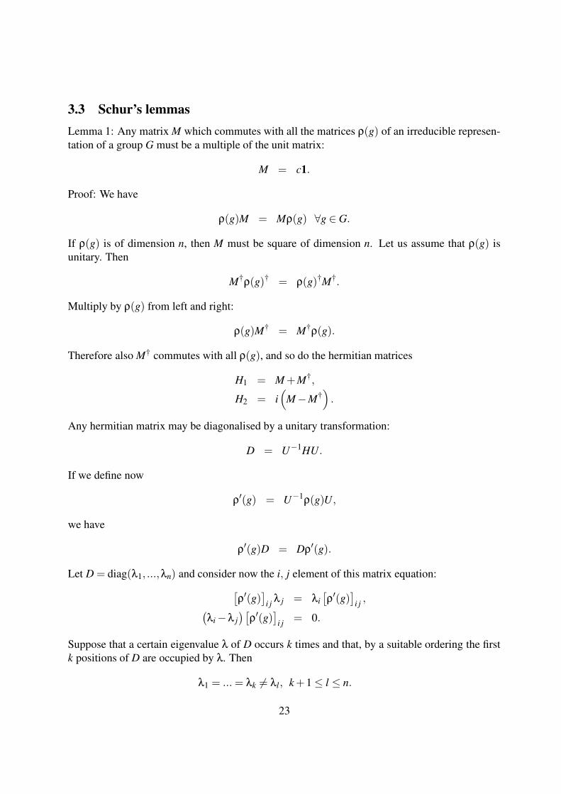
3.3 Schur’s lemmasLemma 1: Any matrix M which commutes with all the matrices ρ(g) of an irreducible represen-tation of a group G must be a multiple of the unit matrix:
M = c1.
Proof: We have
ρ(g)M = Mρ(g) ∀g ∈ G.
If ρ(g) is of dimension n, then M must be square of dimension n. Let us assume that ρ(g) isunitary. Then
M†ρ(g)† = ρ(g)†M†.
Multiply by ρ(g) from left and right:
ρ(g)M† = M†ρ(g).
Therefore also M† commutes with all ρ(g), and so do the hermitian matrices
H1 = M +M†,
H2 = i(
M−M†)
.
Any hermitian matrix may be diagonalised by a unitary transformation:
D = U−1HU.
If we define now
ρ′(g) = U−1ρ(g)U,
we have
ρ′(g)D = Dρ′(g).
Let D = diag(λ1, ...,λn) and consider now the i, j element of this matrix equation:[ρ′(g)
]
i j λ j = λi[ρ′(g)
]
i j ,(λi −λ j
)[ρ′(g)
]
i j = 0.
Suppose that a certain eigenvalue λ of D occurs k times and that, by a suitable ordering the firstk positions of D are occupied by λ. Then
λ1 = ... = λk 6= λl, k +1 ≤ l ≤ n.
23

This implies that[ρ′(g)
]
i j = 0 for 1 ≤ i ≤ k, k +1 ≤ j ≤ n,
or 1 ≤ j ≤ k, k +1 ≤ i ≤ n.
Hence ρ′(g) is of the form(
... 00 ...
)
and is thus reducible, contrary to the initial assumption. Thus if and only if all the eigenvaluesof D are the same ρ′(g) will be irreducible. In other words, D and hence M must be a multipleof the unit matrix.
Lemma 2: If ρ1(g) and ρ2(g) are two irreducible representations of a group G of dimensionsn1 and n2 respectively and if a rectangular matrix M of dimension n1 ×n2 exists sucht that
ρ1(g)M = Mρ2(g), ∀g ∈ G
then either(a) M = 0 or(b) n1 = n2 and detM 6= 0, in which case ρ1(g) and ρ2(g) are equivalent.
Proof: Let us assume without loss of generality that ρ1(g) and ρ2(g) are unitary representations.
M†ρ1(g)† = ρ2(g)†M†,
M†ρ1(g−1) = ρ2(g−1)M†.
Multiply by M from the right:
M†ρ1(g−1)M = ρ2(g−1)M†M.
By assumption ρ1(g−1)M = Mρ2(g−1) and therefore
M†Mρ2(g−1) = ρ2(g−1)M†M.
By lemma 1 we conclude
M†M = λ1.
Consider the case n1 = n2 = n:
det M†M = det M†det M = λn.
If λ 6= 0 then det M 6= 0 and therefore M−1 exists. From ρ1(g)M = Mρ2(g) it follows that
ρ1(g) = Mρ2(g)M−1
24

and ρ1(g) and ρ2(g) are equivalent.
If on the other hand λ = 0 we have
∑k
M†ikMki = 0,
∑k|Mik|2 = 0.
This is only possible for Mik = 0 and hence
M = 0.
To complete the proof we consider the case n1 6= n2. Let us assume n1 < n2. Construct M′ fromM by adding n2 −n1 rows of zeros:
M′ =
(M0
)
M′† =(
M† 0)
We have
M′†M′ = M†M
and thus
det M†M = det M′†M′ = det M′†det M′ = 0.
Hence λ = 0 and M†M = 0. It follows M = 0 as before.
Application: Orthogonality theorem for finite groups. Let G be a finite group and let ρ1 andρ2 be representations of dimension n1 and n2. Then
∑g∈G
ρ1(g)i jρ2(g−1)kl =
0 ρ1 and ρ2 are inequivalent,|G|n1
δilδk j ρ1 and ρ2 are identical,... ρ1 and ρ2 are equivalent, but not identical.
Proof: Assume that ρ1 and ρ2 are inequivalent. Consider
M =1|G| ∑
g∈Gρ1(g)Xρ2(g−1),
where X is an arbitrary n1 ×n2 matrix. Then
ρ(g′)M = ρ(g′)1|G| ∑
g∈Gρ1(g)Xρ2(g−1) =
1|G| ∑
g∈Gρ1(g′g)Xρ2(g−1)
=1|G| ∑
g∈Gρ1(g)Xρ2(g−1g′) =
1|G| ∑
g∈Gρ1(g)Xρ2(g−1)ρ(g′) = Mρ(g′).
25

By Schur’s second lemma we have M = 0, therefore
1|G| ∑
g∈Gρ1(g)i j′X j′k′ρ2(g−1)k′l = 0.
Since X was arbitrary we can take X = δ j j′δkk′ and we have
∑g∈G
ρ1(g)i jρ2(g−1)kl = 0.
Now consider the case where ρ1 and ρ2 are identical: ρ1 = ρ2 = ρ. Take again
M =1|G| ∑
g∈Gρ(g)Xρ(g−1).
One shows again
ρ(g)M = Mρ(g).
Therefore by Schur’s first lemma
1|G| ∑
g∈Gρ(g)i j′X j′k′ρ(g−1)k′l = cδil.
Again take X = δ j j′δkk′:
1|G| ∑
g∈Gρ(g)i jρ(g−1)kl = cδil.
To find c take the trace on both sides:
δk j = cn1,
and therefore
∑g∈G
ρ(g)i jρ(g−1)kl =|G|n1
δk jδil.
Another consequence of Schur’s first lemma: All irreducible representation of an Abelian groupare one-dimensional.
3.4 Representation theory for finite groupsA finite group G admits only finitely many irreducible representations Vi up to isomorphism.
Example: Consider the symmetric group S3, the permutation group of three elements, which
26

is the simplest non-abelian group. This group has two one-dimensional representations: Thetrivial one I and the alternating representation A defined by
gv = sign(g)v.
There is a natural representation, in which S3 acts on C3 by
g · (z1,z2,z3) =(
zg−1(1),zg−1(2),zg−1(3)
)
This representation is reducible: The line spanned by the sum
e1 + e2 + e3
is an invariant sub-space. The complementary sub-space
V = (z1,z2,z3)|z1 + z2 + z3 = 0defines an irreducible representation. This representation is called the standard representation.It can be shown that any representation of S3 can be decomposed into these three irreduciblerepresentations
W = I⊕n1 ⊕A⊕n2 ⊕V⊕n3 .
3.4.1 Characters
Definition:If V is a representation of G, its character χV is the complex-valued function on thegroup defined by
χV (g) = Tr(ρ(g)) .
In particular we have
χV(hgh−1) = χV (g).
Let V and W be representation of G. Then
χV⊕W = χV +χW ,
χV⊗W = χV ·χW ,
χV ∗ = (χV )∗ ,
χ∧2V (g) =12[χV (g)2 −χV (g2)
],
χSym2V(g) =
12[χV (g)2 +χV (g2)
]
Orthogonality theorem for characters: For finite groups we had the orthogonality theorem. Ifwe consider unitary representations and if we make the agreement that if two representations areequivalent, we take them to be identical, the orthogonality theorem can be written as
∑g∈G
ρa(g)i jρb(g)∗lk =|G|n1
δilδk jδab
27

Now we set i = j and sum, and we set l = k and sum:
∑g∈G
χa(g)χb(g)∗ = |G| δab
Since the character is a class function we can write
∑g∈G
= ∑classes κ
nκ,
where nκ denotes the number of elements in the class Cκ. Therefore
∑κ
nκχa(Cκ)χb(Cκ)∗ = |G| δab
Character table:
n1C1 n2C2 n2C2 ...ρ1 χ1(C1) χ1(C2) χ1(C3) ...ρ2 χ2(C1) χ2(C2) χ2(C3) ...ρ3 χ3(C1) χ3(C2) χ3(C3) ...... ... ... ... ...
If we now define
ζaκ =
√nκ|G|χa(Cκ)
we have
∑κ
ζaκζb
κ∗
= δab.
The number of orthogonal vectors corresponds to the number of inequivalent representations.The dimension of the space is given by the number of classes. Therefore the number of inequiv-alent representations is smaller or equal to the number of classes. In fact equality holds.
Criteria for reducibility: Assume that
ρ(g) =M
αaαρα(g)
Then
χ(g) = ∑α
aαχα(g).
Conisder now
1|G|∑g
χ(g)χ(g)∗ = ∑α|aα|2
= 1 ρ irreducible> 1 ρ reducible
28

3.5 Representation theory for Lie groups3.5.1 Irreducible representation of SU(2) and SO(3)
The groups SU(2) and SO(3) have the same Lie algebra:
[Ia, Ib] = iεabcIc.
For SU(2) we can take the Ia’s proportional to the Pauli matrices
I1 =12
(0 11 0
)
, I2 =12
(0 −ii 0
)
, I3 =12
(1 00 −1
)
.
This defines a representation of SU(2) which is called the fundamental representation. (It is nota representation of SO(3).)Quite generally the structure constants provide a representation known as the adjoint or vectorrepresentation:
(Mb)ac = i fabc.
For SU(2) and SO(3):
M1 =
0 0 00 0 −i0 i 0
, M2 =
0 0 i0 0 0−i 0 0
, M3 =
0 −i 0i 0 00 0 0
.
The dimension of the adjoint representation equals the dimension of the parameter space of thegroup and the numbers of generators.
Let us now discus more systematically all irreducible representations.Definition: A Casimir operator is an operator, which commutes with all the generators of thegroup.Example: For SU(2) and SO(3)
I2 = I21 + I2
2 + I23
is a Casimir operator:[I2, Ia
]= 0.
Definition: The rank of a Lie algebra is the number of simultaneously diagonalisable genera-tors.Example 1: SU(2) has rank one, the convention is to take I3 diagonal.Example 2: SU(3) has rank two, in the Gell-Mann representation T3 and T8 are diagonal.
Theorem: The number of independent Casimir operators is equal to the rank of the Lie alge-bra. The proof can be found in many textbooks.
29

Therefore SU(2) has only one Casimir operator.
The eigenvalues of the Casimir operators may be used to label the irreducible representations.The eigenvalues of the diagonal generators can be used to label the basis vectors within a givenirreducible representation.
Example SU(2):
I2 |λ,m〉 = λ |λ,m〉 ,I3 |λ,m〉 = m |λ,m〉 .
Consider(I21 + I2
2)|λ,m〉 =
(I2 − I2
3)|λ,m〉 =
(λ−m2) |λ,m〉 .
Further
〈λ,m| I21 |λ,m〉 = 〈λ,m| I†
1 I1 |λ,m〉 = |I1 |λ,m〉|2 ≥ 0.
A similar consideration applies to 〈λ,m| I22 |λ,m〉. Therefore
λ−m2 ≥ 0.
For a given λ the possible values of m are bounded:
−√
λ ≤ m ≤√
λ
Define
I± =1√2
(I1 ± iI2)
[I3, I±] = ±I±,[I2, I±
]= 0.
The last relation implies(I2I±− I±I2) |λ,m〉 = 0,
I2 (I± |λ,m〉) = λ(I± |λ,m〉) .
Therefore the operators I± don’t change λ. From the commutation relation with I3 we obtain
(I3I±− I±I3) |λ,m〉 = ±I± |λ,m〉 ,I3 (I± |λ,m〉) = (m±1)(I± |λ,m〉) .
30

Therefore I± |λ,m〉 is proportional to |λ,m±1〉 unless zero. Recall that the values of m arebounded, therefore there is a maximal value mmax and a minimal value mmin:
I+ |λ,mmax〉 = 0,
I− |λ,mmin〉 = 0.
Now
I2 = I21 + I2
2 + I23 = I+I−+ I2
3 − I3
= I−I+ + I23 + I3
Therefore
I2 |λ,mmax〉 =(I−I+ + I2
3 + I3)|λ,mmax〉 ,
λ |λ,mmax〉 = mmax (mmax +1) |λ,mmax〉 ,
and
λ = mmax (mmax +1) .
Similar:
I2 |λ,mmin〉 =(I+I− + I2
3 − I3)|λ,mmin〉 ,
λ |λ,mmin〉 = mmin (mmin −1) |λ,mmin〉 ,
and
λ = mmin (mmin −1) .
From
m2max +mmax = m2
min −mmin,
(mmax +mmin)(mmax −mmin +1)︸ ︷︷ ︸
>0
= 0
it follows
mmin = −mmax.
Since the ladder operators raise or lower m by one unit we must have that mmax and mmin differby an integer, therefore
2mmax = integer.
Let us write mmax = j. Then 2 j is an integer and
j = 0,12,1,
32, ...
31

λ = j ( j +1)
Normalisation:
I± |λ,m〉 = A± |λ,m±1〉
With I†± = I∓ we have
|A±|2 = 〈λ,m| I†±I± |λ,m〉 = 〈λ,m| I∓I± |λ,m〉 = 〈λ,m| I2− I3 (I3 ±1) |λ,m〉
and therefore
|A±|2 = j ( j +1)−m(m±1)
Condon-Shortley convention:
A± =√
j ( j +1)−m(m±1).
3.5.2 The Cartan basis
Definition: Suppose a Lie algebra A has a sub-algebra B such that the commutator of any elementof A (T a say) with any element of B (T b say) always lies in B, then B is said to be an ideal of A:
[
T a,T b]
∈ B.
Every Lie algebra has two trivial ideals: A and 0.
A Lie algebra is called simple if it is non-Abelian and has no non-trivial ideals.
A Lie algebra is called semi-simple if it has no non-trivial Abelian ideals.
A Lie algebra is called reductive if it is the sum of a semi-simple and an abelian Lie alge-bra.
A simple Lie algebra is also semi-simple and a semi-simple Lie algebra is also reductive.
Examples: The Lie algebras
su(n),so(n),sp(n)
are simple.Semi-simple Lie algebras are sums of simple Lie algebras:
su(n1)⊕ su(n2).
32

Reductive Lie algebras may have in addition an abelian part:
u(1)⊕ su(2)⊕ su(3).
From Schur’s lemma we know that abelian Lie groups have only one-dimensional irreduciblerepresentations. Therefore let us focus on Lie groups corresponding to semi-simple Lie algebras.A Lie group, which has a semi-simple Lie algebra, is for obvious reasons called semi-simple.We first would like to have a criterion to decide, whether a Lie algebra is semi-simple or not: If
[
T a,T b]
= i f abcT c,
define
gab = f acd f bcd .
A criterion due to Cartan say that a Lie algebra is semi-simple if and only if
det g 6= 0.
For SU(n) we find
gab = CAδab.
Let us now define the Cartan standard form of a Lie algebra. As example suppose we have[T 1,T 2]= 0,
[T 1,T 3] 6= 0,
[T 2,T 3] 6= 0.
If we now make a change of basis
T 1′ = T 1 +T 3, T 2′ = T 2, T 3′ = T 3,
none of the new commutators vanishes. More generally let us assume that
A = in
∑i=1
caT a,
X = in
∑i=1
xaT a,
such that
[A,X ] = iρX .
ρ is called a root of the Lie algebra. We then have
[A,X ] = −icaxb f abcT c = −ρxcT c,(
caxbi f abc −ρxc
)
= 0,(
cai f abc −ρδbc)
xb = 0.
33

For a non-trivial solution we must have
det(
cai f abc −ρδbc)
= 0.
In general the secular equation will give a n-th order polynomial is ρ. Solving for ρ one obtainsn roots. One root may occur more than once. The degree of degeneracy is called the multiplicityof the root.
Theorem (Cartan): If A is chosen sucht that the secular equation has the maximum numberof distince roots, then only the root ρ = 0 is degenerate. Further if r is the multiplicity of thatroot, there exist r linearly independent eigenvectors Hi, which mutually commute
[Hi,H j
]= 0, i, j = 1, ...,r.
r is the rank of the Lie algebra.
Notation: Latin indices for 1, ...,r, e.g. Hi and greek indices for the remaining (n− r) gener-ators Eα (α = 1, ...,n− r).
Example SU(2):[
Ia, Ib]
= iεabcIc.
Take A = iI3:[iI3,X
]= iρX .
Secular equation:
det(
iε3bc −ρδbc)
= 0,∣∣∣∣∣∣
−ρ i 0−i −ρ 00 0 −ρ
∣∣∣∣∣∣
= 0,
−ρ3 +ρ = 0,
ρ(ρ−1) = 0.
Therefore the roots are 0,±1. We have
ρ = 0[I3,X
]= 0 ⇒ X = I3 = H1,
ρ = 1[I3,X
]= X ⇒ X =
1√2
(I1 + iI2)= E1,
ρ = −1[I3,X
]= −X ⇒ X =
1√2
(I1− iI2)= E2.
34
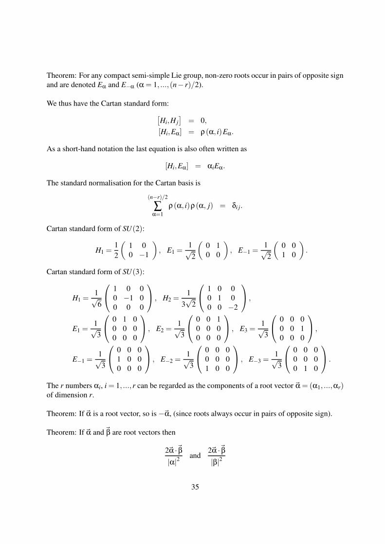
Theorem: For any compact semi-simple Lie group, non-zero roots occur in pairs of opposite signand are denoted Eα and E−α (α = 1, ...,(n− r)/2).
We thus have the Cartan standard form:[Hi,H j
]= 0,
[Hi,Eα] = ρ(α, i)Eα.
As a short-hand notation the last equation is also often written as
[Hi,Eα] = αiEα.
The standard normalisation for the Cartan basis is
(n−r)/2
∑α=1
ρ(α, i)ρ(α, j) = δi j.
Cartan standard form of SU(2):
H1 =12
(1 00 −1
)
, E1 =1√2
(0 10 0
)
, E−1 =1√2
(0 01 0
)
.
Cartan standard form of SU(3):
H1 =1√6
1 0 00 −1 00 0 0
, H2 =1
3√
2
1 0 00 1 00 0 −2
,
E1 =1√3
0 1 00 0 00 0 0
, E2 =1√3
0 0 10 0 00 0 0
, E3 =1√3
0 0 00 0 10 0 0
,
E−1 =1√3
0 0 01 0 00 0 0
, E−2 =1√3
0 0 00 0 01 0 0
, E−3 =1√3
0 0 00 0 00 1 0
.
The r numbers αi, i = 1, ...,r can be regarded as the components of a root vector ~α = (α1, ...,αr)of dimension r.
Theorem: If~α is a root vector, so is −~α, (since roots always occur in pairs of opposite sign).
Theorem: If~α and~β are root vectors then
2~α ·~β|α|2
and2~α ·~β|β|2
35

are integers. Suppose these integers are p and q. Then(
~α ·~β)2
|α|2 |β|2=
pq4
= cos2 θ ≤ 1.
Therefore
pq ≤ 4.
It follows that
cos2 θ = 0,14,12,34,1.
Case θ = 0: This is the trivial case ~α =~β.Case θ = 30: We have pq = 3 and p = 1,q = 3 or p = 3,q = 1. Let us first discuss p = 1,q = 3.This means
2~α ·~β|α|2
= 1,2~α ·~β|β|2
= 3.
Therefore
|α|2
|β|2= 3.
The case p = 3,q = 1 is similar and in summary we obtain
|α|2
|β|2= 3 or
13.
Case θ = 45: We have pq = 2 and p = 1,q = 2 or p = 2,q = 1. It follows
|α|2
|β|2= 2 or
12.
Case θ = 60: We have pq = 1 and p = 1,q = 1. It follows
|α|2
|β|2= 1.
Case θ = 90: In this case p = 0 and q = 0. This leaves the ratio |α|2/|β|2 undetermined.
The cases θ = 120, θ = 135 and θ = 150 are analogous to the ones discussed above.
If~α and~β are root vectors so is
~γ = ~β− 2~α ·~βα2 ~α
Example: The root diagram of SU(3):
36

60
3.5.3 Weights
Let us first recall some basic facts: The rank of a Lie algebra is the number of simultaneouslydiagonalizable generators. In the following we will denote the rank of a Lie algebra by r.
Theorem : The rank of a Lie algebra is equal to the number of independent Casimir opera-tors. (A Casimir operator is an operator, which commutes with all the generators.)
For a Lie algebra of rank r we therefore have r Casimir operators and r simultaneously diag-onalizable generators Hi.
The eigenvalues of the Casimir operators may be used to label the irreducible representations.The eigenvalues of the diagonal generators Hi may be used to label the states within a givenirreducible representation.
Let~λ be a shorthand notation for~λ = (λ1, ...,λr), a set of eigenvalues of Casimir operators andlet ~m be a shorthand notation for ~m = (m1, ...,mr), a set of eigenvalues of the diagonal generators:
Hi|~λ,~m〉 = mi|~λ,~m〉
The vector ~m is called the weight vector.
Example SU(3): Let us consider the fundamental representation. The vector space is spannedby the three vectors
e1 =
100
, e2 =
010
, e3 =
001
.
We have
(H1,H2)e1 =
(1√6,
13√
2
)
e1,
(H1,H2)e2 =
(
− 1√6,
13√
2
)
e2,
(H1,H2)e3 =
(
0,− 23√
2
)
e3.
37

This gives the weight vectors
~m1 =
(1√6
13√
2
)
, ~m2 =
(
− 1√6
13√
2
)
, ~m3 =
(0
−√
23
)
.
and the weight diagram
m1
m2
Consider now the complex conjugate representation of the fundamental representation: If
ρ = exp(iθaT a)
is a representation, then also
ρ∗ = exp(−iθaT a∗) = exp(iθaT a′)
is a representation and we have
T a′ = −T a∗.
It follows that the weights of the complex conjugate representation are negatives of those of thefundamental representation:
m1
m2
Note that in general the complex conjugate representation ρ∗ is inequivalent to ρ. This is incontrast to SU(2), where one can find a S, such that
SIaS−1 = −Ia∗, SρS−1 = ρ∗.
Let us now look at the weights from a more general perspective: The number of different eigen-states with the same weight is called the multiplicity of the weight. A weight is said to be simpleif the multiplicity is 1.
38

For Lie algebras with r ≥ 2, weights are not necessarily simple.
Theorem : Given a weight ~m and a root vector ~α then
2~α ·~mα2
is an integer and
~m′ = ~m− 2~α ·~mα2 ~α
is also a weight vector. ~m and ~m′ are called equivalent weights.(Recall: In the SU(2) case the weight vectors were one-dimensional. Within one irreduciblerepresentation all weights could be obtained from mmax by applying the lowering operator I−.The action of I− corresponds to a shift in the weight proportional to a root vector. For SU(2) allweights within an irreducible representation are equivalent.)
Ordering of weights: The convention for SU(n) is the following: ~m is said to be higher than ~m′
if the rth component of (~m−~m′) is positive (if zero look at the (r−1)th component).
The highest weight of a set of equivalent weights is said to be dominant.(In the case of an irreducible representation of SU(2) the dominant weight is the one with mmax.)
Theorem: For any compact semi-simple Lie algebra there exists for any irreducible represen-tation a highest weight. Furthermore this highest weight is also simple. All other weights ofthe irreducible representation are equivalent to this one. Therefore the highest weights is alsodominant.(Recall: In the SU(2) case we first showed that the values of m are bounded, and then obtainedall other states in the irreducible representation by applying the lowering operator to the statewith mmax.)
Theorem: For every simple Lie algebra of rank r there are r dominant weights ~M(i), calledfundamental dominant weights, such that any other dominant weight ~M is a linear combinationof the ~M(i)
~M =r
∑i=1
ni ~M(i)
where the ni are non-negative integers.
Note that there exists r fundamental irreducible representations, which have the r ~M(i) as theirhighest weight. We can label the irreducible representations by (n1,n2, ...,nr) instead of theeigenvalues of the Casimirs.
39
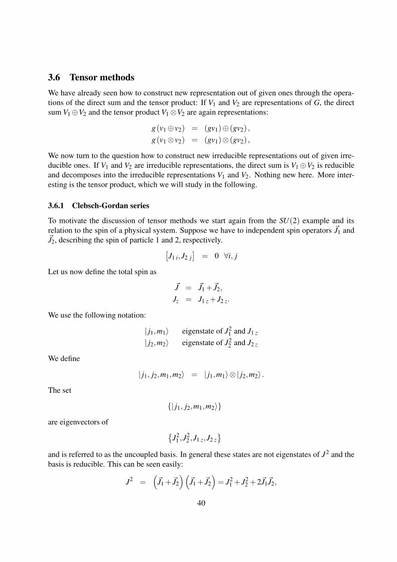
3.6 Tensor methodsWe have already seen how to construct new representation out of given ones through the opera-tions of the direct sum and the tensor product: If V1 and V2 are representations of G, the directsum V1 ⊕V2 and the tensor product V1 ⊗V2 are again representations:
g(v1 ⊕ v2) = (gv1)⊕ (gv2) ,
g(v1 ⊗ v2) = (gv1)⊗ (gv2) ,
We now turn to the question how to construct new irreducible representations out of given irre-ducible ones. If V1 and V2 are irreducible representations, the direct sum is V1 ⊕V2 is reducibleand decomposes into the irreducible representations V1 and V2. Nothing new here. More inter-esting is the tensor product, which we will study in the following.
3.6.1 Clebsch-Gordan series
To motivate the discussion of tensor methods we start again from the SU(2) example and itsrelation to the spin of a physical system. Suppose we have to independent spin operators ~J1 and~J2, describing the spin of particle 1 and 2, respectively.
[J1 i,J2 j
]= 0 ∀i, j
Let us now define the total spin as
~J = ~J1 + ~J2,
Jz = J1 z + J2 z.
We use the following notation:
| j1,m1〉 eigenstate of J21 and J1 z
| j2,m2〉 eigenstate of J22 and J2 z
We define
| j1, j2,m1,m2〉 = | j1,m1〉⊗ | j2,m2〉 .
The set
| j1, j2,m1,m2〉
are eigenvectors of
J21 ,J2
2 ,J1 z,J2 z
and is referred to as the uncoupled basis. In general these states are not eigenstates of J2 and thebasis is reducible. This can be seen easily:
J2 =(
~J1 + ~J2
)(
~J1 + ~J2
)
= J21 + J2
2 +2~J1~J2,
40
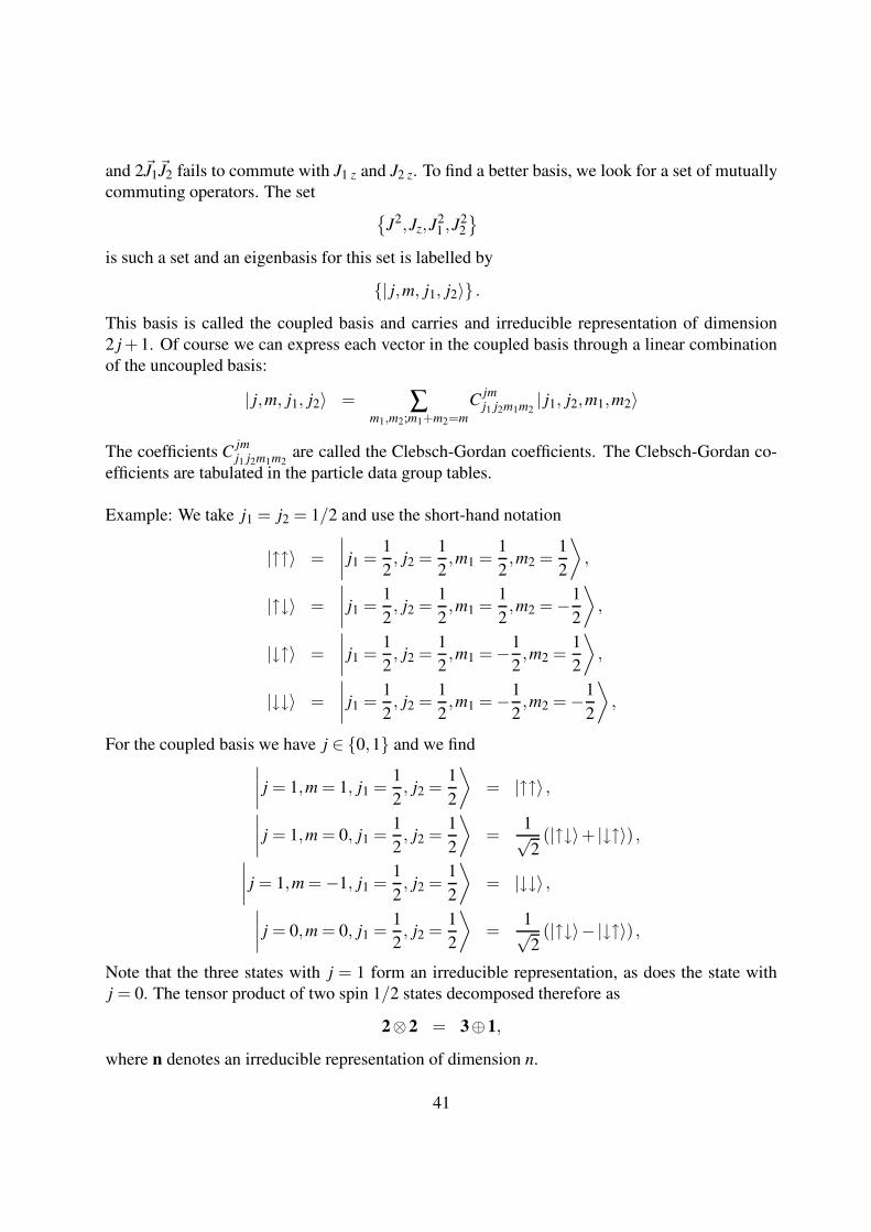
and 2~J1~J2 fails to commute with J1 z and J2 z. To find a better basis, we look for a set of mutuallycommuting operators. The set
J2,Jz,J2
1 ,J22
is such a set and an eigenbasis for this set is labelled by
| j,m, j1, j2〉 .
This basis is called the coupled basis and carries and irreducible representation of dimension2 j +1. Of course we can express each vector in the coupled basis through a linear combinationof the uncoupled basis:
| j,m, j1, j2〉 = ∑m1,m2;m1+m2=m
C jmj1 j2m1m2
| j1, j2,m1,m2〉
The coefficients C jmj1 j2m1m2
are called the Clebsch-Gordan coefficients. The Clebsch-Gordan co-efficients are tabulated in the particle data group tables.
Example: We take j1 = j2 = 1/2 and use the short-hand notation
|↑↑〉 =
∣∣∣∣j1 =
12, j2 =
12,m1 =
12,m2 =
12
⟩
,
|↑↓〉 =
∣∣∣∣j1 =
12, j2 =
12,m1 =
12,m2 = −1
2
⟩
,
|↓↑〉 =
∣∣∣∣j1 =
12, j2 =
12,m1 = −1
2,m2 =
12
⟩
,
|↓↓〉 =
∣∣∣∣j1 =
12, j2 =
12,m1 = −1
2,m2 = −1
2
⟩
,
For the coupled basis we have j ∈ 0,1 and we find∣∣∣∣j = 1,m = 1, j1 =
12, j2 =
12
⟩
= |↑↑〉 ,∣∣∣∣j = 1,m = 0, j1 =
12, j2 =
12
⟩
=1√2
(|↑↓〉+ |↓↑〉) ,
∣∣∣∣j = 1,m = −1, j1 =
12, j2 =
12
⟩
= |↓↓〉 ,∣∣∣∣j = 0,m = 0, j1 =
12, j2 =
12
⟩
=1√2
(|↑↓〉− |↓↑〉) ,
Note that the three states with j = 1 form an irreducible representation, as does the state withj = 0. The tensor product of two spin 1/2 states decomposed therefore as
2⊗2 = 3⊕1,
where n denotes an irreducible representation of dimension n.
41

3.6.2 The Wigner-Eckart theorem
Let us make a small detour and discuss the Wigner-Eckart theorem. We have already seen thatthe group SU(2) is generated by the three generators
J1 =1√2
(I1 + iI2) ,
J0 = I3,
J−1 =1√2
(I1 − iI2) .
J−1,J0,J1 define the spherical basis. The generators transform under SU(2) as the adjointrepresentation. For SU(2) the adjoint representation is the 3 representation. Let us denote thematrix representation of such a transformation by
D( j)m′m,
where 2 j +1 denotes the dimension of the representation and m′,m = − j, ...,0, ..., j. The spher-ical basis transforms in this notation as
(Jq′)′
= D(1)q′q Jq.
We can now generalise this construction and define a tensor operator T kq of rank k as a set of
(2k +1) operators which transform irreducibly under the group as(
T kq′
)′= D(k)
q′qT kq .
The set J−1,J0,J1 is therefore a tensor operator of rank 1. An equivalent definition for a tensoroperator is a set of (2k +1) operators satisfying
[
I3,T kq
]
= qT kq ,
[
I±,T kq
]
=√
(k∓q)(k±q+1)T kq±1 =
√
k(k +1)−q(q±1)T kq .
We can now state the Wigner-Eckart theorem:
⟨
j′m′∣∣∣T k
q
∣∣∣ jm
⟩
=1√
2 j′ +1C j′m′
jkmq
⟨
j′∣∣∣
∣∣∣T k∣∣∣
∣∣∣ j⟩
.
The important point is that the double bar matrix element 〈 j′||T k|| j〉 is independent of m, m′ andq. The dependence on m, m′ and q is entirely given by the Clebsch-Gordan coefficients C j′m′
jkmq.
42

3.6.3 Young diagrams
We have seen that the tensor product of two fundamental representations of SU(2) decomposesas
2⊗2 = 3⊕1,
into a direct sum of irreducible representations. We generalise this now to general irreduciblerepresentations of SU(N).
Definition: A Young diagram is a collection of m boxes 2 arranged in rows and left-justified. Tobe a legal Young diagram, the number of boxes in a row must not increase from top to bottom.An example for a Young diagram is
Let us denote the number of boxes in row j by λ j. Then a Young diagram is a partition of mdefined by the numbers (λ1,λ2, ...,λn) subject to
λ1 +λ2 + ...+λn = m,
λ1 ≥ λ2 ≥ ... ≥ λn.
The example diagram above therefore corresponds to
(λ1,λ2,λ3,λ4) = (4,2,1,1)
The number of rows is denoted by n. For SU(N) we consider only Young diagrams with n ≤ N.
Let us further define (n−1) numbers p j by
p1 = λ1 −λ2,
p2 = λ2 −λ3,
...
pn−1 = λn−1 −λn−2.
The example above has
(p1, p2, p3) = (2,1,0)
Correspondence between Young diagrams and irreducible representations: Recall from the lastlecture that we could label any irreducible representation of a simple Lie algebra of rank r byeither the r eigenvalues of the Casimir operators or by the r numbers (p1, ..., pr) appearing when
43
expressing the dominant weight of the representation in terms of the fundamental dominantweights:
~M =r
∑i=1
pi ~M(i)
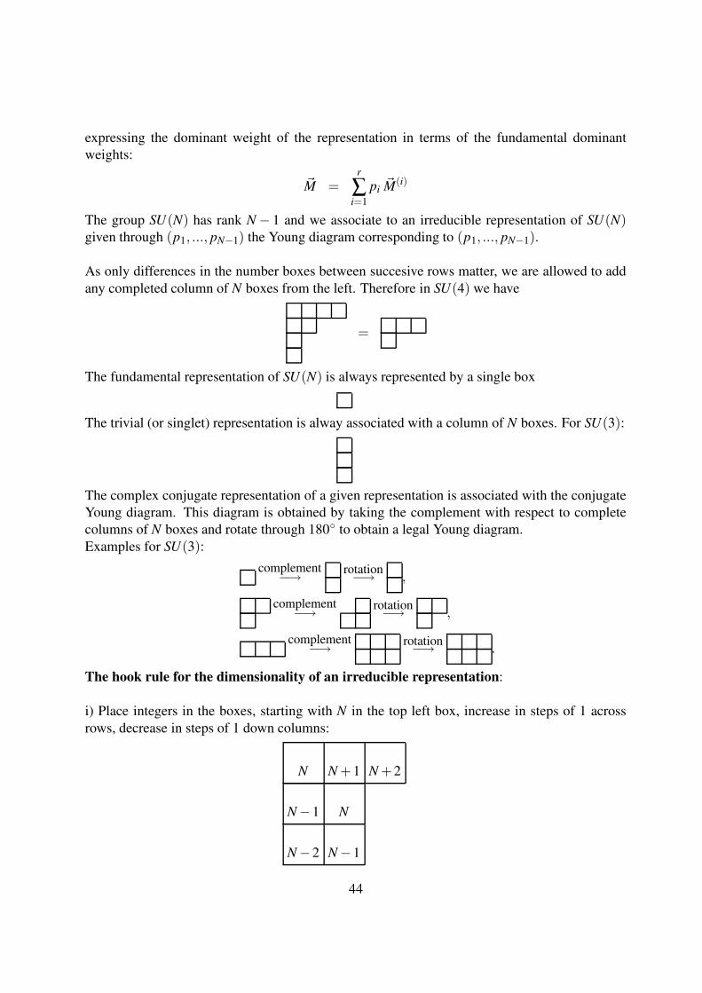
The group SU(N) has rank N − 1 and we associate to an irreducible representation of SU(N)given through (p1, ..., pN−1) the Young diagram corresponding to (p1, ..., pN−1).
As only differences in the number boxes between succesive rows matter, we are allowed to addany completed column of N boxes from the left. Therefore in SU(4) we have
=
The fundamental representation of SU(N) is always represented by a single box
The trivial (or singlet) representation is alway associated with a column of N boxes. For SU(3):
The complex conjugate representation of a given representation is associated with the conjugateYoung diagram. This diagram is obtained by taking the complement with respect to completecolumns of N boxes and rotate through 180 to obtain a legal Young diagram.Examples for SU(3):
complement−→ rotation−→ ,
complement−→ rotation−→ ,
complement−→ rotation−→ .
The hook rule for the dimensionality of an irreducible representation:
i) Place integers in the boxes, starting with N in the top left box, increase in steps of 1 acrossrows, decrease in steps of 1 down columns:
N N +1 N +2
N −1 N
N −2 N −1
44

ii) Compute the numerator as the product of all integers.
iii) The denominator is given by multiplying all hooks of a Young diagram. A hook is thenumber of boxes that one passes through on entering the tableau along a row from the right hnadside and leaving down a column.
Some examples for SU(3):
3 42 : dim =
2 ·3 ·41 ·3 ·1 = 8,
3 4 5 : dim =3 ·4 ·51 ·2 ·3 = 10,
3 4 52 3 4 : dim =
2 ·3 ·4 ·3 ·4 ·51 ·2 ·3 ·2 ·3 ·4 = 10.
Rules for tensor products: We now give rules for tensor products of irreducible representationsrepresented by Young diagrams. As an example we take in SU(3)
⊗
i) Label the boxes of the second factor by row, e.g. a, b, c, ...:
−→ a ab
.
ii) Add the boxes with the a’s from the lettered diagram to the right-hand ends of the rows of theunlettered diagram to form all possible legitimate Young diagrams that have no more than one aper column.
a a ,a
a
Note that the diagram
aa
is not allowed since it has one column with two a’s.
iii) Repeat the same with the b’s, then with the c’s, etc.
a a b , a ab
,a a
b,
a b
a
ab
a
45
Note that the diagram
a
ab
is not allowed for SU(3), since it has more than 3 rows.
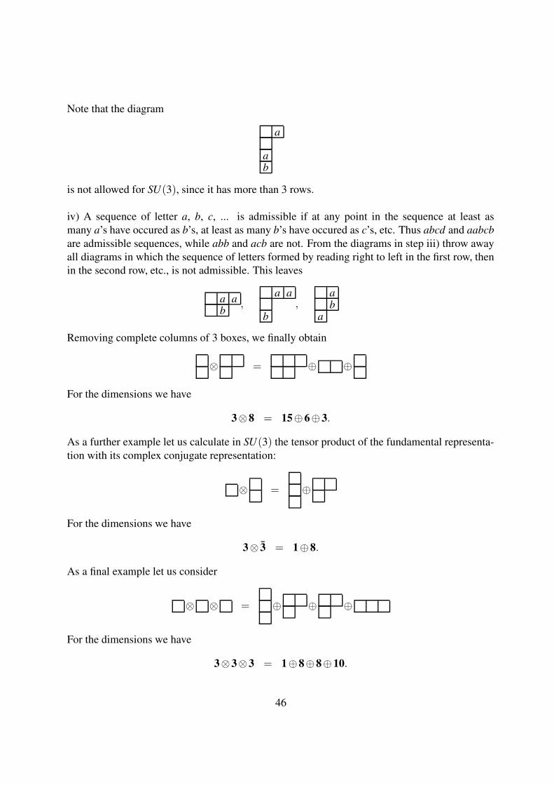
iv) A sequence of letter a, b, c, ... is admissible if at any point in the sequence at least asmany a’s have occured as b’s, at least as many b’s have occured as c’s, etc. Thus abcd and aabcbare admissible sequences, while abb and acb are not. From the diagrams in step iii) throw awayall diagrams in which the sequence of letters formed by reading right to left in the first row, thenin the second row, etc., is not admissible. This leaves
a ab
,a a
b,
ab
a
Removing complete columns of 3 boxes, we finally obtain
⊗ = ⊕ ⊕
For the dimensions we have
3⊗8 = 15⊕6⊕3.
As a further example let us calculate in SU(3) the tensor product of the fundamental representa-tion with its complex conjugate representation:
⊗ = ⊕
For the dimensions we have
3⊗ 3 = 1⊕8.
As a final example let us consider
⊗ ⊗ = ⊕ ⊕ ⊕
For the dimensions we have
3⊗3⊗3 = 1⊕8⊕8⊕10.
46
4 The classification of semi-simple Lie algebrasRecall: For a semi-simple Lie algebra g of dimension n snd r we had the Cartan standard form
[Hi,H j
]= 0,
[Hi,Eα] = αiEα,
with generators Hi, i = 1, ...,r as well as the generators Eα and E−α with α = 1, ...,(n− r)/2.
The generators Hi generate an Abelian sub-algebra of g. This sub-algebra is called the Car-tan sub-algebra of g.
The r numbers αi, i = 1, ...,r are the components of the root vector ~α = (α1, ...,αr).
We have already seen that if if ~α and~β are root vectors so is
~γ = ~β− 2~α ·~βα2 ~α
Let us now put this a little bi more formally. For any root vector α we define a mapping Wα fromthe set of root vectors to the set of root vectors by
Wα(β) = ~β− 2~α ·~βα2 ~α
Wα can be described as the reflection by the plane Ωα perpendicular to α. It is clear that thismapping is an involution: After two reflections one obtains the original root vector again. Theset of all these mappings Wα generates a group, which is called the Weyl group.
Since Wα maps a root vector to another root vector, we have the following theorem:
Theorem: The set of root vectors is invariant under the Weyl group.
Actually, a more general result holds: We have seen that if ~m is a weight and if ~α is a rootvector then
Wα (~m) = ~m− 2~α ·~mα2 ~α
is again a weight vector. Therefore we can state that the following theorem:
Theorem: The set of weights of any representation of g is invariant under the Weyl group.
The previous theorem is a special case of this one, as the root vectors are just the weights ofthe adjoint representation.
47

For the weights we defined an ordering. ~m is said to be higher than ~m′ if the rth componentof (~m− ~m′) is positive (if zero look at the (r− 1)th component). This applies equally well toroots.
Definition: A root vectors~α is called positive, if ~α >~0.
Therefore the set of non-zero root vectors R decomposes into
R = R+∪R−,
where R+ denotes the positive roots and R− denotes the negative roots.
Definition: The (closed) Weyl chamber relative to a given ordering is the set of points ~x inthe r-dimensional space of root vectors, such that
2~x ·~αα2 ≥ 0 ∀~α ∈ R+.
Example: The Weyl chamber for SU(3):
Let us further recall that if~α and~β are root vectors then
2~α ·~β|α|2
and2~α ·~β|β|2
are integers. This restricts the angle between two root vectors to
0,30,45,60,90,120,135,150,180
For θ = 30 or θ = 150 the ratio of the length of the two root vectors is
|α|2
|β|2= 3 or
13.
For θ = 45 or θ = 135 the ratio of the length of the two root vectors is
|α|2
|β|2= 2 or
12.
48

For θ = 60 or θ = 120 the ratio of the length of the two root vectors is
|α|2
|β|2= 1.
Let us summarise: The root system R of a Lie algebra has the following properties:
1. R is a finite set.
2. If~α ∈ R, then also −~α ∈ R.
3. For any~α ∈ R the reflection Wα maps R to itself.
4. If~α and~β are root vectors then 2~α ·~β/ |α|2 is an integer.
This puts strong constraints on the geometry of a root system. Let us now try to find all possibleroot systems of rank 1 and 2. For rank 1 the root vectors are one-dimensional and the onlypossibility is
A1:
This is the root system of SU(2). For rank 2 we first note that due to property (3) the anglebetween two roots must be the same for any pair of adjacent roots. It will turn out that any of thefour angles 90, 60, 45 and 30 can occur. Once this angle is specified, the relative lengths ofthe roots are fixed except for the case of right angles. Let us start with the case θ = 90. Up torescaling the root system is
A1 ×A1:
This corresponds to SU(2)× SU(2). This group is semi-simple, but not simple. In general, thedirect sum of two root systems is again a root system. A root system which is not a direct sum iscalled irreducible. An irreducible root system corresponds to a simple group. We would like toclassify the irreducible root systems.
For the angle θ = 60 we have
A2
49
This is the root system of SU(3).
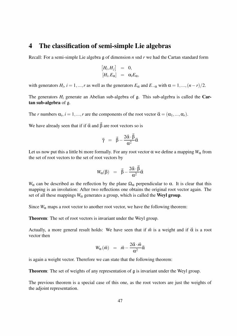
For the angle θ = 45 we have
B2:
This is the root system of SO(5).
Finally, for θ = 30 we have
G2:
This is the root system of the exceptional Lie group G2.
4.1 Dynkin diagramsLet us try to reduce further the data of a root system. We already learned that with the help of anordering we can divide the root vectors into a disjoint union of positive and negative roots:
R = R+∪R−.
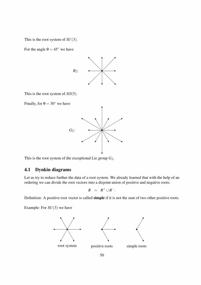
Definition: A positive root vector is called simple if it is not the sum of two other positive roots.
Example: For SU(3) we have
root system positive roots simple roots
50

The angle between the two simple roots is θ = 120.
The Dynkin diagram of the root system is constructed by drawing one node for each sim-ple root and joining two nodes by a number of lines depending on the angle θ between the tworoots:
no lines if θ = 90
one line if θ = 120
two lines if θ = 135
three lines if θ = 150
When there is one line, the roots have the same length. If two roots are connected by two or threelines, an arrow is drawn pointing from the longer to the shorter root.
Example: The Dynkin diagram of SU(3) is
4.2 The classificationSemi-simple groups are a direct product of simple groups. For a compact group, all unitary rep-resentations are finite dimensional.Real compact semi-simple Lie algebras g are in one-to-one correspondence (up to isomorphisms)with complex semi-simple Lie algebras g
C obtained as the complexification of g. Therefore theclassification of real compact semi-simple Lie algebras reduces to the classification of complexsemi-simple Lie algebras.
Theorem: Two complex semi-simple Lie algebras are isomorphic if and only if they have thesame Dynkin diagram.
Theorem: A complex semi-simple Lie algebra is simple if and only if its Dynkin diagram isconnected.
We have the following classification:
• An ∼= SL(n+1,C)
· · ·α1 α2 α3 αn−1 αn
• Bn ∼= SO(2n+1,C)
· · ·α1 α2 α3 αn−1 αn
51
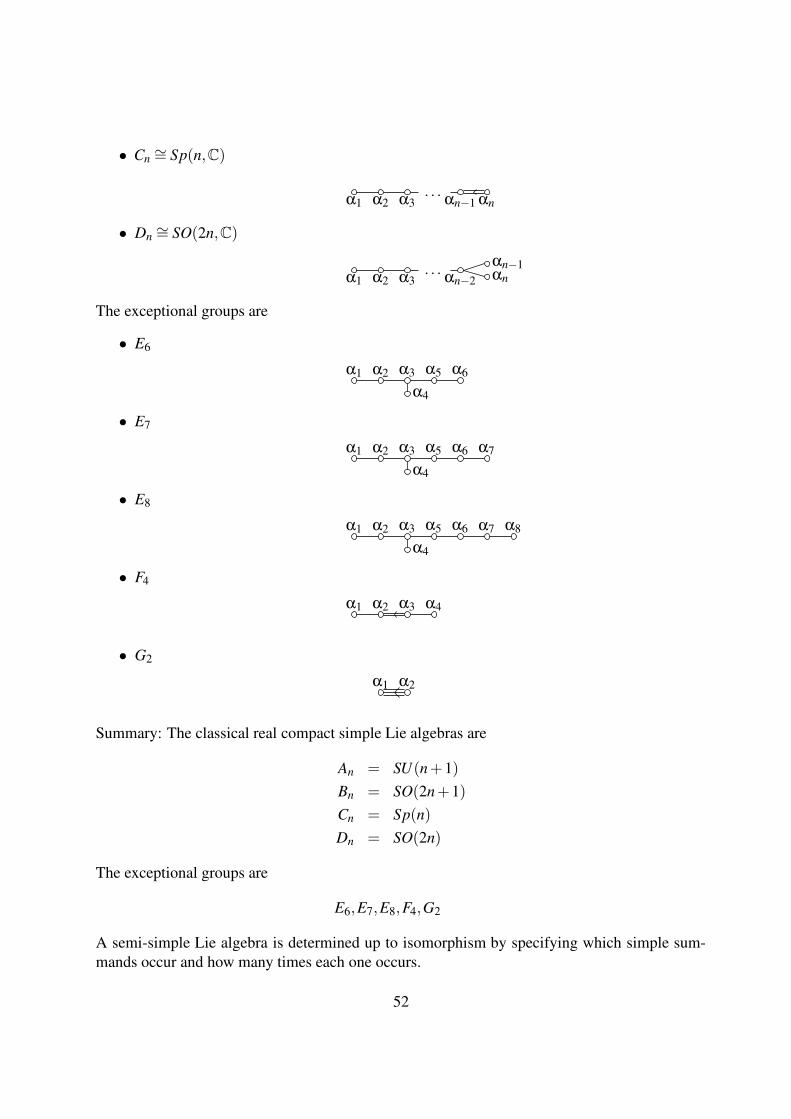
• Cn ∼= Sp(n,C)
· · ·α1 α2 α3 αn−1 αn
• Dn ∼= SO(2n,C)
· · ·α1 α2 α3 αn−2
αn−1αn
The exceptional groups are
• E6
α1 α2 α3 α5 α6
α4
• E7
α1 α2 α3 α5 α6 α7
α4
• E8
α1 α2 α3 α5 α6 α7 α8
α4
• F4
α1 α2 α3 α4
• G2
α1 α2
Summary: The classical real compact simple Lie algebras are
An = SU(n+1)
Bn = SO(2n+1)
Cn = Sp(n)
Dn = SO(2n)
The exceptional groups are
E6,E7,E8,F4,G2
A semi-simple Lie algebra is determined up to isomorphism by specifying which simple sum-mands occur and how many times each one occurs.
52

4.3 Proof of the classificationRecall: The root system R of a Lie algebra has the following properties:
1. R is a finite set.
2. If~α ∈ R, then also −~α ∈ R.
3. For any~α ∈ R the reflection Wα maps R to itself.
4. If~α and~β are root vectors then 2~α ·~β/ |α|2 is an integer.
With the help of an ordering we can divide the root vectors into a disjoint union of positive andnegative roots:
R = R+∪R−.
A positive root vector is called simple if it is not the sum of two other positive roots.
The angle between two simple roots is either 90, 120, 135 or 150
The Dynkin diagram of the root system is constructed by drawing one node for each sim-ple root and joining two nodes by a number of lines depending on the angle θ between the tworoots:
no lines if θ = 90
one line if θ = 120
two lines if θ = 135
three lines if θ = 150
When there is one line, the roots have the same length. If two roots are connected by two or threelines, an arrow is drawn pointing from the longer to the shorter root.
Theorem: The only possible connected Dynkin diagrams are the ones listed in the previoussection.
To prove this theorem it is sufficient to consider only the angles between the simple roots, therelative length do not enter the proof.
Such diagrams, without the arrows to indicate the relative lengths, are called Coxeter diagrams.Define a diagram of n nodes, with each pair connected by 0, 1, 2 or 3 lines, to be admissible ifthere are n independent unit vectors~e1, ...,~en in a Euclidean space with the angle between~ei and~e j as follows:
53
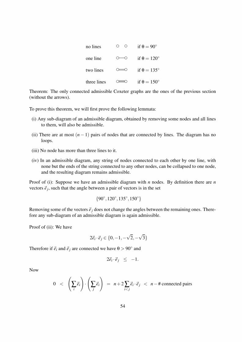
no lines if θ = 90
one line if θ = 120
two lines if θ = 135
three lines if θ = 150
Theorem: The only connected admissible Coxeter graphs are the ones of the previous section(without the arrows).
To prove this theorem, we will first prove the following lemmata:
(i) Any sub-diagram of an admissible diagram, obtained by removing some nodes and all linesto them, will also be admissible.
(ii) There are at most (n− 1) pairs of nodes that are connected by lines. The diagram has noloops.
(iii) No node has more than three lines to it.
(iv) In an admissible diagram, any string of nodes connected to each other by one line, withnone but the ends of the string connected to any other nodes, can be collapsed to one node,and the resulting diagram remains admissible.
Proof of (i): Suppose we have an admissible diagram with n nodes. By definition there are nvectors~e j, such that the angle between a pair of vectors is in the set
90,120,135,150
Removing some of the vectors~e j does not change the angles between the remaining ones. There-fore any sub-diagram of an admissible diagram is again admissible.
Proof of (ii): We have
2~ei ·~e j ∈ 0,−1,−√
2,−√
3
Therefore if~ei and~e j are connected we have θ > 90 and
2~ei ·~e j ≤ −1.
Now
0 <
(
∑i~ei
)
·(
∑j~ei
)
= n+2 ∑i< j
~ei ·~e j < n−# connected pairs
54

Therefore
# connected pairs < n.
Connecting n nodes with (n− 1) connections (of either 1, 2 or 3 lines) implies that there are noloops.
Proof of (iii): We first note that(2~ei ·~e j
)2= # number of lines between~ei and~e j.
Consider the node~e1 and let~ei, i = 2, ..., j bet the nodes connected to~e1. We want to show
j
∑i=2
(2~e1 ·~ei)2 < 4.
Since there are no loops, no pair of ~e2,...,~e j is connected. Therefore ~e2, ..., ~e j are perpendicularunit vectors. Further, by assumption~e1,~e2,...,~e j are linearly independent vectors. Therefore~e1 isnot in the span of~e2,...,~e j. It follows
1 = (~e1 ·~e1)2 >
j
∑i=2
(~e1 ·~ei)2
and therefore
j
∑i=2
(~e1 ·~ei)2 < 1.
Proof of (iv):1 2 r
→
If~e1, ...,~er are the unit vectors corresponding to the string of nodes as indicated above, then
~e′ = ~e1 + ...+~er
is a unit vector since
~e′ ·~e′ = (~e1 + ...+~er)2 = r +2~e1 ·~e2 ++2~e2 ·~e3 + ...++2~er−1 ·~er
= r− (r−1) = 1.
Further~e′ satisfies the same conditions with respect to the other vectors since~e′ ·~e j is either~e1 ·~e jor~er ·~e j.
55

With the help of these lemmata we can now prove the original theorem:
From (iii) it follows that the only connected diagram with a triple line is G2.
Further we cannot have a diagram with two double lines, otherwise we would have a sub-diagram, which we could contract as
... →
contradicting again (iii). By the same reasoning we cannot have a diagram with a double lineand a triple node:
... →
Again this contradicts (iii).
To finish the case with double lines, we rule out the diagram1 2 3 4 5
Consider the vectors
~v =~e1 +2~e2, ~w = 3~e3 +2~e4 +~e5.
We find
(~v ·~w)2 = 18, |~v|2 = 3, |~w|2 = 6.
This violates the Cauchy-Schwarz inequality
(~v ·~w)2 < |~v|2 · |~w|2 .
By a similar reasoning one rules out the following (sub-) graphs with single lines:
These sub-diagrams rules out all graphs not in the list of the previous section. To finish the proofof the theorem it remains to show that all graphs in the list are admissible. This is equivalent
56

to show that for each Dynkin diagram in the list there exists a corresponding Lie algebra. (Thesimple root vectors of such a Lie algebra will then have automatically the corresponding anglesof the Coxeter diagram.)
To prove the existence it is sufficient to give for each Dynkin diagram an example of a Lie alge-bra corresponding to it. For the four families An, Bn, Cn and Dn we have already seen that theycorrespond to the Lie algebras of SU(n + 1), SO(2n + 1), Sp(n) and SO(2n) (or SL(n + 1,C),SO(2n + 1,C), Sp(n,C) and SO(2n,C) in the complex case). In addition one can write downexplicit matrix representations for the Lie algebras corresponding to the five exceptional groupsE6, E7, E8, F4 and G2.
Finally for the uniqueness let us recall the following theorem: Two complex semi-simple Liealgebras are isomorphic if and only if they have the same Dynkin diagram.
57