Lidar data in water resources applications data in water resources applications Paola Passalacqua CE 394K 3 Guest Lecture, November 15th, 2012

Lidar data in water

resources applications

Paola Passalacqua

CE 394K 3 Guest Lecture, November 15th, 2012

Airborne Lidar

Airborne laser altimetry technology (lidar, Light Detection And Ranging) provides high-

resolution topographical data, which can significantly contribute to a better representation of

land surface. A valuable characteristic of this technology, which marks advantages over the

traditional topographic survey techniques, is the capability to derive a high-resolution Digital

Terrain Model (DTM) from the last pulse LiDAR data by filtering the vegetation points (Slatton

et al., 2007).

Slide courtesy of Dr. Paolo Tarolli, University of Padova, Italy


Airborne Lidar

x,y,z


Airborne Lidar

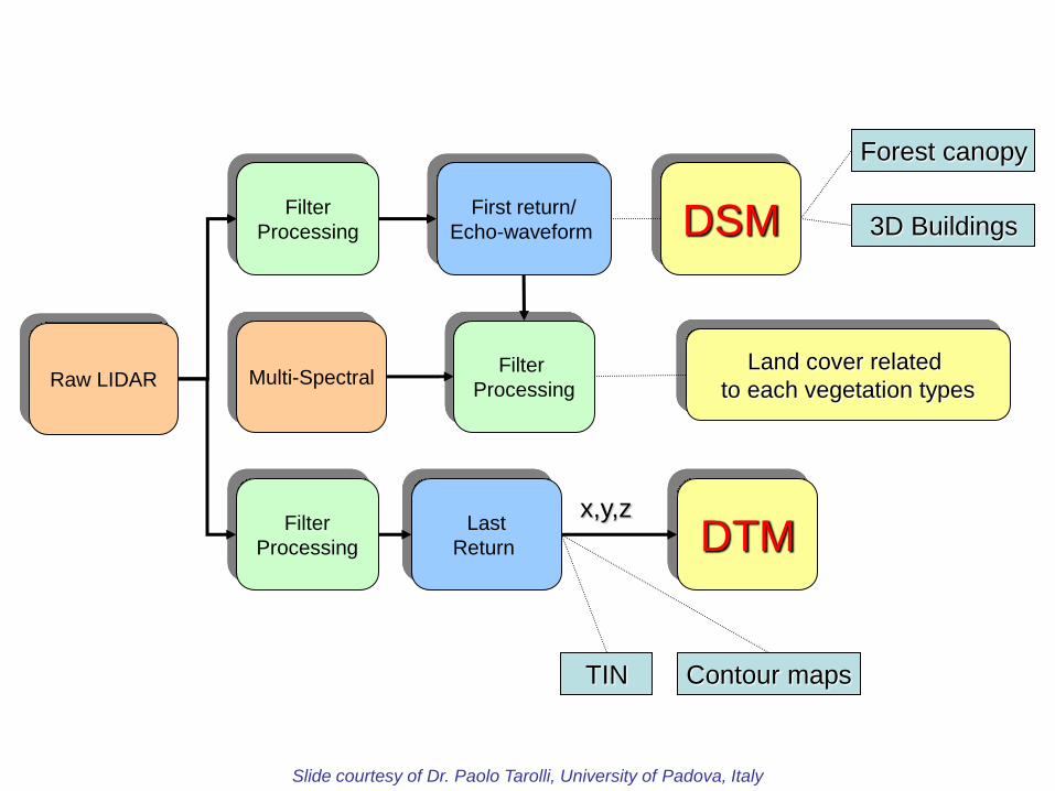
First return/

Echo-waveform

Last

Return DTM

Raw LIDAR

Filter

Processing

Filter

Processing

Filter

Processing Multi-Spectral

x,y,z

DSM

Land cover related

to each vegetation types

Forest canopy

3D Buildings

Contour maps TIN


Topographic Lidar

Green LiDAR λ = 532 nm + λ =1064 nm

λ = 1064 nm

It is important to remember that the

deep water surfaces normally do not

reflect the signal: however this is not

true in case of presence of floating

sediments or when using bathymetric

lidar. The bathymetric lidar, that is

based on the same principles as

topographic lidar, emits laser beams

in two wavelengths: an infrared (1064

nm) and a green one (532 nm). The

infrared wavelength is reflected on the

water surface, while the green one

penetrates the water and is reflected

by the bottom surface or other objects

in the water. Due to this reason the

bathymetric lidar is also called green

lidar.


Fonte: www.optech.ca

During optimal environment condition,

when the water is clear, the green lidar

survey may reach 50 m water depth

with an horizontal accuracy of ±2.5 m,

and vertical accuracy of ±0.25 m. This

technology is growing fast, and some of

the first applications in rivers are coming

out (Hilldale and Raff, 2008; McKean et

al., 2009).


Example 1: Le Sueur River basin

Minnesota River Basin

Le Sueur

Lake Pepin

Le Sueur River located in south-central Minnesota,

covers an area of 2880 km2 (87% row-crop

agriculture)

Provides ~ 24%-30% of the TSS entering the

Minnesota River

Minnesota River major source of sediment for Lake

Pepin (~85% of TSS load)

Turbidity and related nutrients levels of Lake Pepin

are far in excess of EPA standards

State of Minnesota required to determine the

sources of pollution and take management and

policy actions

NCED Research

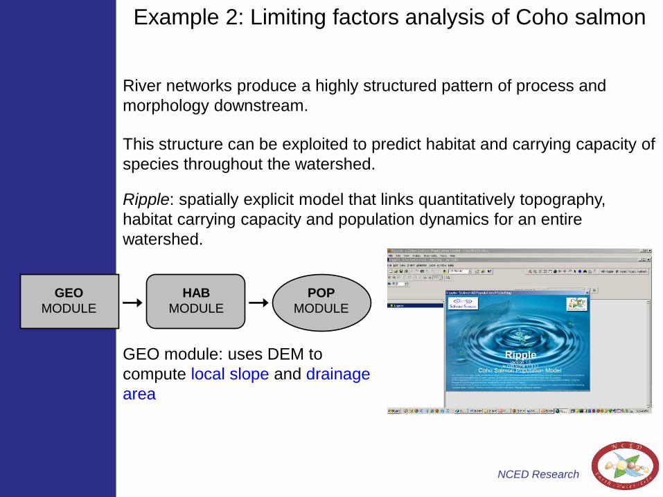
Example 2: Limiting factors analysis of Coho salmon

River networks produce a highly structured pattern of process and

morphology downstream.

This structure can be exploited to predict habitat and carrying capacity of

species throughout the watershed.

Ripple: spatially explicit model that links quantitatively topography,

habitat carrying capacity and population dynamics for an entire

watershed.

GEO

MODULE

HAB

MODULE

POP

MODULE

GEO module: uses DEM to

compute local slope and drainage

area

NCED Research

Example 3: Drainage density as a signature of climate

The problem of resolution: Strong

discrepancy between channels as

mapped in the field and as deduced from

topographic maps (Morisawa, [1957;

1961]; Schneider [1961]).

Schneider, W.J., J. Geophys. Res., 1961

Melton, M.A., ONR Tech Report, 1957

• Climate exerts a quantifiable control over the

degree of channel dissection

• Lithology and relief are important cofactors

Digital elevation data

Grigno basin, Italy

Resolution 30 m x 30 m

Data source: University of Padova

Tanaro basin, Italy



Tirso basin, Italy



Data resolution available until recently 30-100 m.

Rio Cordon basin, Selva di Cadore, Italy


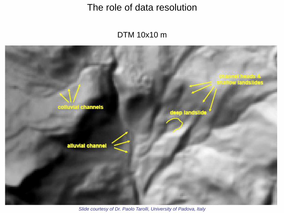
The role of data resolution

DTM 10x10 m


DTM 1x1 m


The role of data resolution

Lidar DTMs: Solving the resolution problem?

• Availability of meter and sub-meter

resolution topographic data

• Topographic patterns can be resolved

over large areas at resolutions

commensurate with the scale of

governing processes

• Importance of objective extraction of

geomorphic feature

Opportunity to measure drainage density

Challenges in geomorphic feature extraction

• Channel initiation

• Identification of accurate centerline

• Presence of roads and bridges

• Artificial drainage ditches

• Small signal to noise ratio

• Identification of channel banks

• Measurement of bluffs

GeoNet: NCED toolbox for channel network

extraction

GeoNet: Nonlinear filtering

1. Nonlinear filtering: Enhance features of interest, while smoothing

small scale features. Perona and Malik [1990]

, , , ,th x y t c x y t h

2/1

1

hc

Smooth

Keep

Channel

Bumps

GeoNet: Statistical signature of geomorphic transitions

2. Skeleton of likely channelized pixels: Set of pixels with curvature

above threshold, identified from quantile-quantile plot of curvature.

thk

The deviation of the pdf from Gaussian can be interpreted as transition

from hillslope to valley [Lashermes et al,. 2007].

Channel extraction: geodesics

b

a

Outlet

Channel

head

The cost function ψ represents the cost of traveling between point a and

point b in terms of a function of area (A), slope (S), curvature (κ) and

skeleton (Skel):

Age

SkelSAf

1.,.

),,,(

1

2. Geodesic minimization: Channels are extracted as paths of

minimum cost

Channel initiation and channel disruptions

Passalacqua, P., P. Tarolli, and E. Foufoula-Georgiou, Water Resour. Res, 2010

Flat lands and channel morphology

• Le Sueur River major source of sediment to the Minnesota River.

• Both listed as impaired for turbidity by USEPA.

• Need to identify sediment sources

Roads and ditches

Identification of likely channelized pixels in engineered

landscapes

Passalacqua, P., P. Belmont, and E. Foufoula-Georgiou, Water Resour. Res., 2012

Curvature analysis to distinguish channels and roads

𝜅 = 𝛻 ∙𝛻ℎ

𝛻ℎ

𝛾 = 𝛻2ℎ


Differentiating natural versus artificial features


Channel network extraction and bridge crossings


Automatic extraction of channel morphology

• Automatic extraction of channel cross-section

• Detection of bank location

• Identification of geomorphic bankfull water surface elevation

• Measurements of channel width and of bank and bluff height

Height 60 m

Source: P. Belmont

Source: C. Jennings

Automatic extraction of channel morphology


Codependence of vegetation and drainage density

Field mapped channel heads on slope

gradient map (Imaizumi et al. [2010]).

GeoNet drainage delineation.

Preliminary results: Codependence of vegetation and

drainage density

Preliminary results: Codependence of vegetation and

drainage density

Multi-resolution analysis of landscapes to understand

landscape forming processes characteristic scales

The first scaling break represents

the length scale of the highly

convex regions(i.e. the ridges)

The second scaling break

represents the hillslope length

scale.

Slide courtesy of Harish Sangireddy, UT Austin

Six test sites were studied for

testing the methodology.

The data for the test sites was

obtained from TNRIS


Feature extraction from point cloud

Site 1 has only streams and surrounding farmlands

dry stream



Site 2 has roads, streams, marshy areas, small culvert and drains by the

roadside

road

stream

marshy

area



stream

Probable

floodplain

Detects points around the water gaps and maps the geometry of stream properly



drain

road

tree

farmland

When the elevation difference is very small in the region, the model identifies all

low lying areas as water surfaces

Site 5 Slide courtesy of Harish Sangireddy, UT Austin


Acknowledgements

Work supported by:

NSF EAR-0120914 (NCED)

NSF EAR-0835789

NSF BCS-1063231/1063228 (PIs Stark

and Passalacqua)

Collaborators (in random order):

Tien Do Trung, Colin Stark, Guillermo

Sapiro, Bill Dietrich, Efi Foufoula-Georgiou,

Nachiket Gokhale, Paolo Tarolli, Patrick

Belmont , Harish Sangireddy, David

Maidment, Yuichi S. Hayakawa, Fumitoshi

Imaizumi, Tsuyoshi Hattanji, Lin Zhou.

Documents

Lidar data in water resources applications data in water resources applications Paola Passalacqua CE 394K 3 Guest Lecture, November 15th, 2012