Embed Size (px)
Citation preview
LiDAR-Camera Calibration using 3D-3D Pointcorrespondences
Ankit Dhall1, Kunal Chelani2, Vishnu Radhakrishnan3, K. Madhava Krishna4
1Vellore Institute of Technology, Chennai2Birla Institute of Technology and Science, Hyderabad
3Veermata Jijabai Technological Institute, Mumbai4International Institute of Information and Technology, Hyderabad
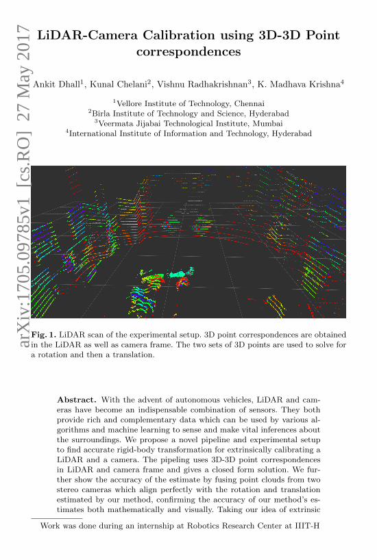
Fig. 1. LiDAR scan of the experimental setup. 3D point correspondences are obtainedin the LiDAR as well as camera frame. The two sets of 3D points are used to solve fora rotation and then a translation.
Abstract. With the advent of autonomous vehicles, LiDAR and cam-eras have become an indispensable combination of sensors. They bothprovide rich and complementary data which can be used by various al-gorithms and machine learning to sense and make vital inferences aboutthe surroundings. We propose a novel pipeline and experimental setupto find accurate rigid-body transformation for extrinsically calibrating aLiDAR and a camera. The pipeling uses 3D-3D point correspondencesin LiDAR and camera frame and gives a closed form solution. We fur-ther show the accuracy of the estimate by fusing point clouds from twostereo cameras which align perfectly with the rotation and translationestimated by our method, confirming the accuracy of our method’s es-timates both mathematically and visually. Taking our idea of extrinsic
Work was done during an internship at Robotics Research Center at IIIT-H
arX
iv:1
705.
0978
5v1
[cs
.RO
] 2
7 M
ay 2
017
2 A. Dhall, K. Chelani, V. Radhakrishnan, K.M. Krishna
LiDAR-camera calibration forward, we demonstrate how two cameraswith no overlapping field-of-view can also be calibrated extrinsically us-ing 3D point correspondences. The code has been made available asopen-source software in the form of a ROS package.
Keywords: extrinsic calibration, LiDAR, camera, rigid-body transfor-mation
1 Introduction
Robotic platforms, both autonomous and remote controlled, use multiple sen-sors such as IMUs, multiple cameras and range sensors. Each sensor providesdata in a complementary modality. For instance, cameras provide rich color andfeature information which can be used by state-of-the-art algorithms to detectobjects of interest (pedestrians, cars, trees, etc.). Range sensors have gained alot of popularity recently despite being more expensive and also contain movingparts. These can provide rich structural information and if correspondence canbe drawn between the camera and the LiDAR, when a pedestrian is detected inan image, it’s exact 3D location can be estimated and be used by an autonomouscar to avoid obstacles and prevent accidents.
Multiple sensors are employed to provide redundant information which re-duces the chance of having erroneous measurements. In the above cases, it isessential to obtain data from various sensors with respect to a single frame ofreference so that data can be fused and redundancy can be leveraged. Markerbased[2] as well as automatic calibration for LiDAR and cameras has been pro-posed but methods and experiments discussed in these use the high-density, moreexpensive LiDAR and do not extend very well when a lower-density LiDAR, suchas the VLP-16 is used.
We propose a very accurate and repeatable method to estimate extrinsiccalibration parameters in the form of 6 degrees-of-freedom between a cameraand a LiDAR.
2 Sensors and General Setup
The method we propose makes use of sensor data from a LiDAR and a camera.The intrinsic parameters of the camera should be known before starting theLiDAR-camera calibration process.
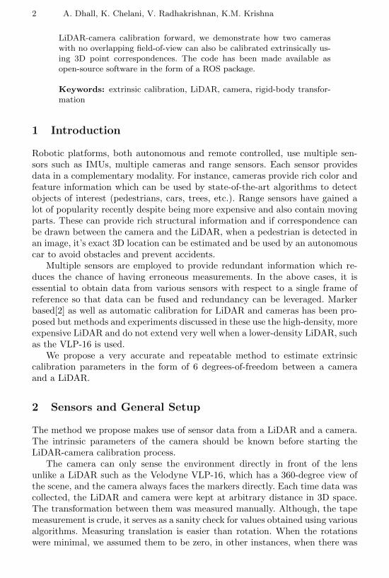
The camera can only sense the environment directly in front of the lensunlike a LiDAR such as the Velodyne VLP-16, which has a 360-degree view ofthe scene, and the camera always faces the markers directly. Each time data wascollected, the LiDAR and camera were kept at arbitrary distance in 3D space.The transformation between them was measured manually. Although, the tapemeasurement is crude, it serves as a sanity check for values obtained using variousalgorithms. Measuring translation is easier than rotation. When the rotationswere minimal, we assumed them to be zero, in other instances, when there was
LiDAR-Camera Calibration using 3D-3D Point correspondences 3
considerable rotation in the orientation of the sensors, we measured distancesand estimated the angles roughly using trigonometry.
3 Using 2D-3D correspondences
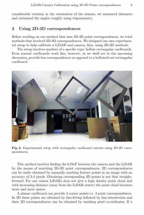
Before working on our method that uses 3D-3D point correspondences, we triedmethods that involved 2D-3D correspondences. We designed our own experimen-tal setup to help calibrate a LiDAR and camera, first, using 2D-3D methods.
The setup involves markers of a specific type: hollow rectangular cardboards.Even normal cardboards work fine, however, as we shall see in the upcomingdiscussion, provide less correspondences as opposed to a hollowed out rectangularcardboard.
Fig. 2. Experimental setup with rectangular cardboard cutouts using 2D-3D corre-spondences.
This method involves finding the 6-DoF between the camera and the LiDARby the means of matching 2D-3D point correspondences. 2D correspondencescan be easily obtained by manually marking feature points in an image with anaccuracy of 3-4 pixels. Obtaining corresponding 3D points is not that straight-forward. For one reason LiDARs does not give a high density point cloud andwith increasing distance (away from the LiDAR center) the point cloud becomesmore and more sparse.
A planar cardboard can provide 4 corner points i.e. 4 point correspondences.In 3D these points are obtained by line-fitting followed by line-intersection andtheir 2D correspondences can be obtained by marking pixel co-ordinates. If a
4 A. Dhall, K. Chelani, V. Radhakrishnan, K.M. Krishna
hollowed out rectangular cardboard is used, it provides 8 3D-2D point correspon-dences: 4 corners on the outer rectangle and 4 corners on the inner rectangle;doubling the correspondences, allowing for more data points with lesser numberof boards. Such a setup allows to have enough data to run a RaNSaC version ofPnP algorithms and also will help reduce noisy data, in general.
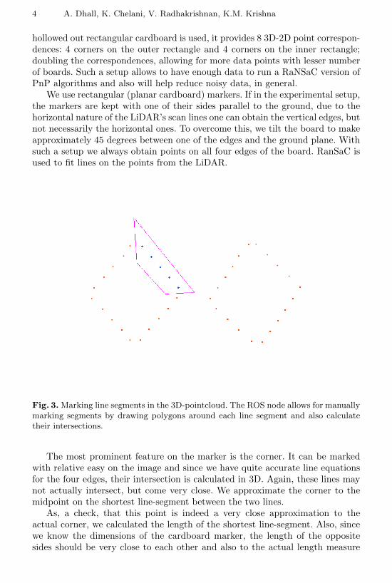
We use rectangular (planar cardboard) markers. If in the experimental setup,the markers are kept with one of their sides parallel to the ground, due to thehorizontal nature of the LiDAR’s scan lines one can obtain the vertical edges, butnot necessarily the horizontal ones. To overcome this, we tilt the board to makeapproximately 45 degrees between one of the edges and the ground plane. Withsuch a setup we always obtain points on all four edges of the board. RanSaC isused to fit lines on the points from the LiDAR.
Fig. 3. Marking line segments in the 3D-pointcloud. The ROS node allows for manuallymarking segments by drawing polygons around each line segment and also calculatetheir intersections.
The most prominent feature on the marker is the corner. It can be markedwith relative easy on the image and since we have quite accurate line equationsfor the four edges, their intersection is calculated in 3D. Again, these lines maynot actually intersect, but come very close. We approximate the corner to themidpoint on the shortest line-segment between the two lines.
As, a check, that this point is indeed a very close approximation to theactual corner, we calculated the length of the shortest line-segment. Also, sincewe know the dimensions of the cardboard marker, the length of the oppositesides should be very close to each other and also to the actual length measure
LiDAR-Camera Calibration using 3D-3D Point correspondences 5
by tape. We consistently observed that the distance between two line-segmentswas of the order 10−4 meters and the error between the edge lengths was about1 centimeter on average.
Collecting data over multiple experiments, we observed that the edges areextremely close and the corner and intersection are at most off by 0.68 mm onaverage. An average absolute deviation of 1cm is observed between the expectedand estimated edge lengths of the cardboard markers. With the above two ob-servations one can conclude that the intersections are indeed a very accurateapproximation of the corner in 3D.
uv1
=
fx γ cx0 fx cy0 0 1
∗r11 r12 r13 t1r21 r22 r23 t2r31 r32 r33 t3
∗xyz1
(1)
Using hollowed out markers, we obtained 20 corner points: 2 hollow rectangu-lar markers (8+8 points) and one solid rectangular marker (4 points) increasingthe number of point correspondences from our initial experiments.
Perspective n-Point (PnP) finds the rigid-body transformation between a setof 2D-3D correspondences. Equation 1 shows how the 3D points are projectedafter applying the [R|t] which is estimated by PnP. Equation 2 represents thegeneral cost-function to solve such a problem.
arg minR∈SO(3),t∈R3
||P (RX + t)− x||2 (2)
where,
P is the projection operation from 3D to 2D on the image planeX represents points in 3Dx represents points in 2D
To begin with, we started with PnP and E-PnP[6]. The algorithms seemedto minimize the error; and with manually filtering (refer to table 1) the points(by visualizing the outliers) we were able to lower the back-projection error to1.88 pixels on average. However, one did not observe the [R|t] close to the valuesmeasure by measuring tape between the camera and LiDAR.
In a previous experiment, when the LiDAR and camera were quite close(12cm apart) we ran the E-PnP with 12 points and did not obtain the expectedvalues. We observed that we got an error of 10cm and if our expected value isaround that measure of granularity then we can expect to obtain noisy values.In subsequent experiments the the camera and LiDAR were kept even fartherapart so that the influence of any error is mitigated.
While examining the data, we found that there were some noisy data pointswho were contributing to a large back projection error. We ran a modified E-PnP with a RanSaC algorithm on top. This would in theory ensure that noisydata is not considered while calculating the rigid body transformation betweenthe camera and the LIDAR. RanSaC selects a random subset of the data, fits
6 A. Dhall, K. Chelani, V. Radhakrishnan, K.M. Krishna
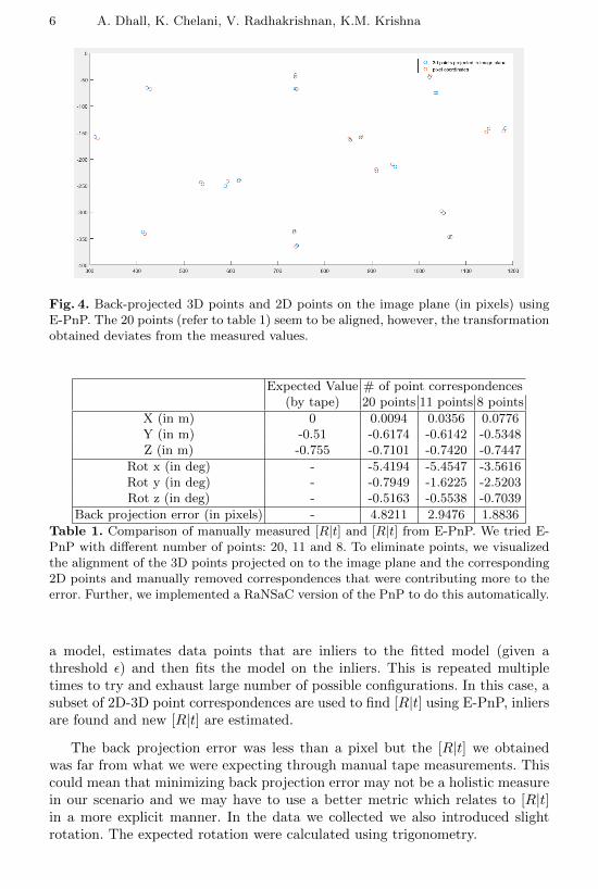
Fig. 4. Back-projected 3D points and 2D points on the image plane (in pixels) usingE-PnP. The 20 points (refer to table 1) seem to be aligned, however, the transformationobtained deviates from the measured values.
Expected Value # of point correspondences(by tape) 20 points 11 points 8 points
X (in m) 0 0.0094 0.0356 0.0776Y (in m) -0.51 -0.6174 -0.6142 -0.5348Z (in m) -0.755 -0.7101 -0.7420 -0.7447
Rot x (in deg) - -5.4194 -5.4547 -3.5616Rot y (in deg) - -0.7949 -1.6225 -2.5203Rot z (in deg) - -0.5163 -0.5538 -0.7039
Back projection error (in pixels) - 4.8211 2.9476 1.8836
Table 1. Comparison of manually measured [R|t] and [R|t] from E-PnP. We tried E-PnP with different number of points: 20, 11 and 8. To eliminate points, we visualizedthe alignment of the 3D points projected on to the image plane and the corresponding2D points and manually removed correspondences that were contributing more to theerror. Further, we implemented a RaNSaC version of the PnP to do this automatically.
a model, estimates data points that are inliers to the fitted model (given athreshold ε) and then fits the model on the inliers. This is repeated multipletimes to try and exhaust large number of possible configurations. In this case, asubset of 2D-3D point correspondences are used to find [R|t] using E-PnP, inliersare found and new [R|t] are estimated.
The back projection error was less than a pixel but the [R|t] we obtainedwas far from what we were expecting through manual tape measurements. Thiscould mean that minimizing back projection error may not be a holistic measurein our scenario and we may have to use a better metric which relates to [R|t]in a more explicit manner. In the data we collected we also introduced slightrotation. The expected rotation were calculated using trigonometry.
LiDAR-Camera Calibration using 3D-3D Point correspondences 7
rot data Expected Value E-PnP RanSaC E-PnP(by tape) 20 points 20 points
X (in m) 0.785 1.0346 1.0422Y (in m) -0.52 -0.557 -0.5883Z (in m) -0.69 -0.393 -0.4078
Rot x (in deg) unmeasurable -5.82 -6.613Rot y (in deg) -15 -17.54 -17.703Rot z (in deg) 2.6 3.27 3.126
Back projection error (in pixels) - 4.35 0.5759
Table 2. Comparison of [R|t] tape measurement, E-PnP, RaNSaC E-PnP. With 20correspondences, we initialize with 15 initial points and tried 10000 different random2D-3D point correspondence selections followed by RaNSaC and E-PnP.
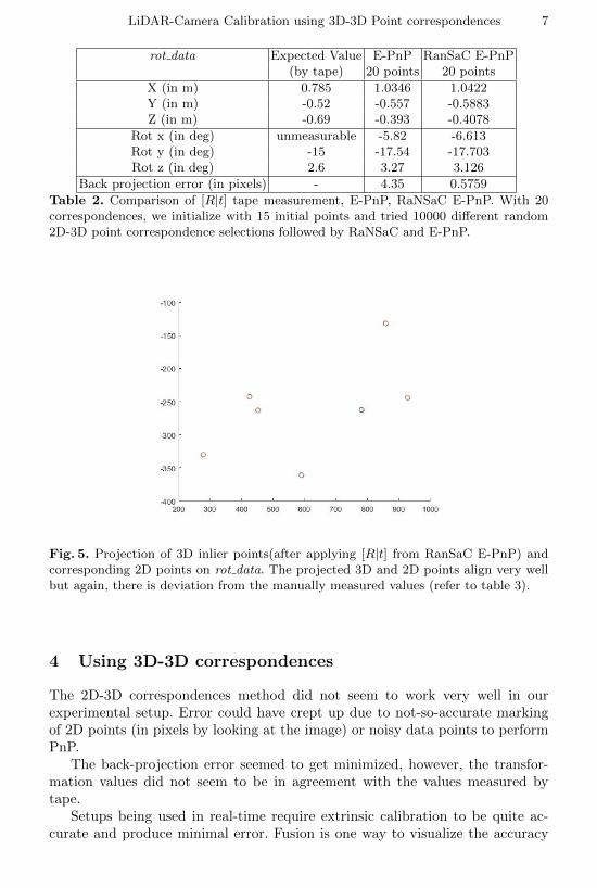
Fig. 5. Projection of 3D inlier points(after applying [R|t] from RanSaC E-PnP) andcorresponding 2D points on rot data. The projected 3D and 2D points align very wellbut again, there is deviation from the manually measured values (refer to table 3).
4 Using 3D-3D correspondences
The 2D-3D correspondences method did not seem to work very well in ourexperimental setup. Error could have crept up due to not-so-accurate markingof 2D points (in pixels by looking at the image) or noisy data points to performPnP.
The back-projection error seemed to get minimized, however, the transfor-mation values did not seem to be in agreement with the values measured bytape.
Setups being used in real-time require extrinsic calibration to be quite ac-curate and produce minimal error. Fusion is one way to visualize the accuracy
8 A. Dhall, K. Chelani, V. Radhakrishnan, K.M. Krishna
of the extrinsic calibration parameters. Bad calibration can result in fused datato have hallucinations in the form of duplication of objects in the fused pointclouds due to bad alignment.
One such application requiring real-time fusion from multiple sensors is au-tonomous driving. Bad calibration can result in erroneous fused data, which canbe fatal for the car as well as nearby cars, pedestrians and property.
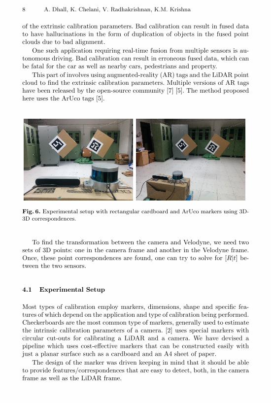
This part of involves using augmented-reality (AR) tags and the LiDAR pointcloud to find the extrinsic calibration parameters. Multiple versions of AR tagshave been released by the open-source community [7] [5]. The method proposedhere uses the ArUco tags [5].
Fig. 6. Experimental setup with rectangular cardboard and ArUco markers using 3D-3D correspondences.
To find the transformation between the camera and Velodyne, we need twosets of 3D points: one in the camera frame and another in the Velodyne frame.Once, these point correspondences are found, one can try to solve for [R|t] be-tween the two sensors.
4.1 Experimental Setup
Most types of calibration employ markers, dimensions, shape and specific fea-tures of which depend on the application and type of calibration being performed.Checkerboards are the most common type of markers, generally used to estimatethe intrinsic calibration parameters of a camera. [2] uses special markers withcircular cut-outs for calibrating a LiDAR and a camera. We have devised apipeline which uses cost-effective markers that can be constructed easily withjust a planar surface such as a cardboard and an A4 sheet of paper.
The design of the marker was driven keeping in mind that it should be ableto provide features/correspondences that are easy to detect, both, in the cameraframe as well as the LiDAR frame.
LiDAR-Camera Calibration using 3D-3D Point correspondences 9
Shape and Size The rectangular cardboard can be of any arbitrary size. Theexperiments we performed used a Velodyne VLP-16[3] which has only 16 rings ina single scan, a handful as compared to higher density LiDARs (32 and 64 ringsper scan). For a low density LiDAR, if the dimensions of the board are small andthe LiDAR is kept farther than a specific distance, the number of rings hittingthe board become low (2 to 3 rings resulting in only 2 to 3 points on an edge) ,making it very difficult to fit lines on the edges (using RanSaC).
The boards used in the experiments had length/breadth ranging between45.0-55.0 centimeters. Keeping the LiDAR about 2.0 meters away from boardwith these dimensions, enough points were registered on the board edges tofit lines, calculate intersections and run the whole pipeline smoothly. It is rec-ommended that before you run the pipeline, ensure that there are considerablenumber of points on the edge of the boards in the pointcloud. Any planar surfacecan be used: cardboards, wood or acrylic sheets. Cardboards are light-weight andcan be hung easily.
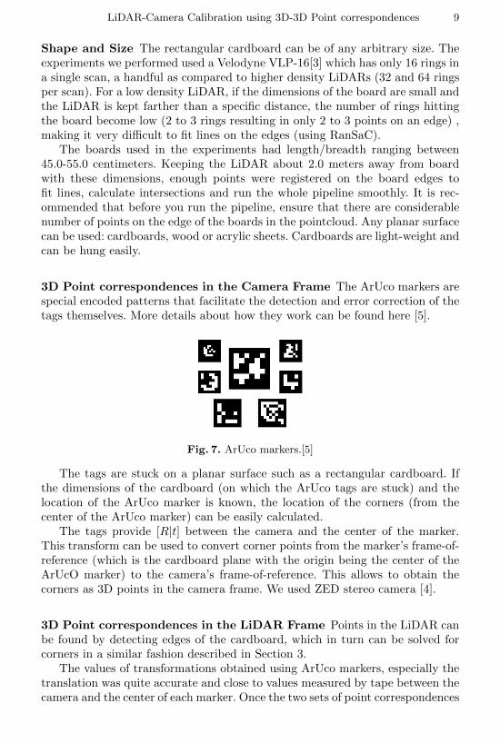
3D Point correspondences in the Camera Frame The ArUco markers arespecial encoded patterns that facilitate the detection and error correction of thetags themselves. More details about how they work can be found here [5].
Fig. 7. ArUco markers.[5]
The tags are stuck on a planar surface such as a rectangular cardboard. Ifthe dimensions of the cardboard (on which the ArUco tags are stuck) and thelocation of the ArUco marker is known, the location of the corners (from thecenter of the ArUco marker) can be easily calculated.
The tags provide [R|t] between the camera and the center of the marker.This transform can be used to convert corner points from the marker’s frame-of-reference (which is the cardboard plane with the origin being the center of theArUcO marker) to the camera’s frame-of-reference. This allows to obtain thecorners as 3D points in the camera frame. We used ZED stereo camera [4].
3D Point correspondences in the LiDAR Frame Points in the LiDAR canbe found by detecting edges of the cardboard, which in turn can be solved forcorners in a similar fashion described in Section 3.
The values of transformations obtained using ArUco markers, especially thetranslation was quite accurate and close to values measured by tape between thecamera and the center of each marker. Once the two sets of point correspondences
10 A. Dhall, K. Chelani, V. Radhakrishnan, K.M. Krishna
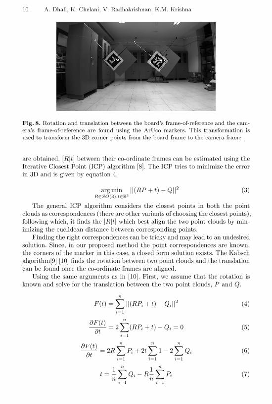
Fig. 8. Rotation and translation between the board’s frame-of-reference and the cam-era’s frame-of-reference are found using the ArUco markers. This transformation isused to transform the 3D corner points from the board frame to the camera frame.
are obtained, [R|t] between their co-ordinate frames can be estimated using theIterative Closest Point (ICP) algorithm [8]. The ICP tries to minimize the errorin 3D and is given by equation 4.
arg minR∈SO(3),t∈R3
||(RP + t)−Q||2 (3)
The general ICP algorithm considers the closest points in both the pointclouds as correspondences (there are other variants of choosing the closest points),following which, it finds the [R|t] which best align the two point clouds by min-imizing the euclidean distance between corresponding points.
Finding the right correspondences can be tricky and may lead to an undesiredsolution. Since, in our proposed method the point correspondences are known,the corners of the marker in this case, a closed form solution exists. The Kabschalgorithm[9] [10] finds the rotation between two point clouds and the translationcan be found once the co-ordinate frames are aligned.
Using the same arguments as in [10]. First, we assume that the rotation isknown and solve for the translation between the two point clouds, P and Q.
F (t) =
n∑i=1
||(RPi + t)−Qi||2 (4)
∂F (t)
∂t= 2
n∑i=1
(RPi + t)−Qi = 0 (5)
∂F (t)
∂t= 2R
n∑i=1
Pi + 2t
n∑i=1
1− 2
n∑i=1
Qi (6)
t =1
n
n∑i=1
Qi −R1
n
n∑i=1
Pi (7)
LiDAR-Camera Calibration using 3D-3D Point correspondences 11
t = Q̄−RP̄ (8)
Substituting the result of equation 8 in objective function 4.
R = arg minR∈SO(3)
||(R(Pi − P̄ )− (Qi − Q̄)||2 (9)
let,X = (Pi − P̄ ) , X ′ = RX and Y = (Qi − Q̄) (10)
then, the objective becomes,
n∑i=1
||X ′i − Yi||2 = Tr((X ′ − Y )T (X ′ − Y )) (11)
using properties of the trace of a matrix, the above equation can be simplifiedas,
Tr((X ′ − Y )T (X ′ − Y )) = Tr(X ′TX ′) + Tr(Y TY )− 2Tr(Y TX)) (12)
since, the R is an orthonormal matrix, it preserves lengths i.e. |X ′i|2 = |Xi|2,
Tr((X ′ − Y )T (X ′ − Y )) =
n∑i=1
(|Xi|2 + |Yi|2)− 2Tr(Y TX ′) (13)
re-writing the objective function by eliminating terms that do not involve R,
R = arg maxR∈SO(3)
Tr(Y TX ′) (14)
substituting the value of X ′ and using property of the trace,
Tr(Y TX ′) = Tr(Y TRX) = Tr(XY TR) (15)
using SVD on XY T = UDV T ,
Tr(XY TR) = Tr(UDV TR) = Tr(DV TRU) =
3∑i=1
divTi Rui (16)
let, M = V TRU , then,
Tr(Y TX ′) =
3∑i=1
diMii ≤3∑
i=1
di (17)
M is a product of orthonormal matrices and is an orthonormal matrix as wellwith det(M) = +/ − 1. The length of each column vector in M is equal to oneand each component of a vector is less than or equal to one. Now, to maximizethe above equation, let each Mii = 1, forcing the remaining components of the
12 A. Dhall, K. Chelani, V. Radhakrishnan, K.M. Krishna
vector to zero to satisfy the unit vector constraint. Thus, M = I, an identitymatrix.
M = I =⇒ V TRU = I =⇒ R = V UT (18)
to ensure, that R is a proper rotation matrix, i.e. R ∈ SO(3), we need to makesure that det(R) = +1. If the R obtained from equation 18 has det(R) = −1 weneed to find R such that Tr(Y TX ′) takes the second largest value possible.
Tr(Y TX ′) = d1M11 + d2M22 + d3M33 where d1 ≥ d2 ≥ d3 and |Mii| ≤ 1 (19)
the second largest value of the term in equation 19 occurs when M11 = M22 =+1 and M33 = −1. Taking into account the above,
R = UCV T (20)
where C is a correction matrix,
C =
1 0 00 1 00 0 sign(det(UV T )) · 1
(21)
4.2 Incorporating multiple scans
In our initial experiments, we observed that even in a closed room where theboards are as stationary as can be, the pointcloud visualized in Rviz shows thatthe points (from the LiDAR), on the contrary, are not stationary and there is asmall amount of position shift between two instants.
To reduce any noise that might creep up we further propose to collect mul-tiple samples of rotations and translations (using the method discussed above).Rotations and translation estimated over multiple runs can be used to obtain amore accurate and less noisy rigid-body transformation that transforms pointsfrom the LiDAR frame to the camera frame. Multiple sensor data, is collectedover N iterations, keeping the positions of the LiDAR and camera fixed.
From each one of the N runs we estimate the rotation and translation. Wecan average the N observed translation vectors,
t̄ =1
N
N∑i=1
tveci (22)
where tveci ∈ R3 and t̄ is the average translation between the two sensors.Taking average of rotation matrices is not very straight-forward, so we trans-
form them to quaternions, compute the average quaternion in R4 and then con-vert it back to rotation matrix.
r =1
N
N∑i=1
rveci (23)
LiDAR-Camera Calibration using 3D-3D Point correspondences 13
r̄ =r
||r||(24)
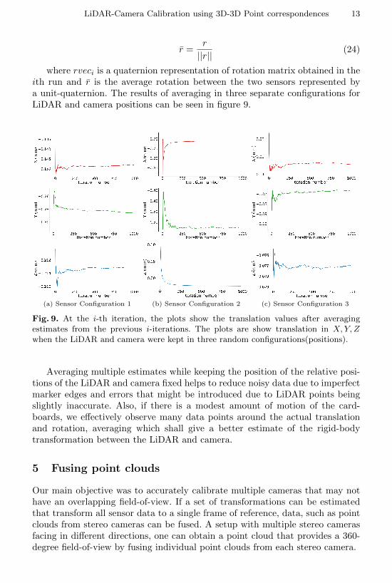
where rveci is a quaternion representation of rotation matrix obtained in theith run and r̄ is the average rotation between the two sensors represented bya unit-quaternion. The results of averaging in three separate configurations forLiDAR and camera positions can be seen in figure 9.
(a) Sensor Configuration 1 (b) Sensor Configuration 2 (c) Sensor Configuration 3
Fig. 9. At the i-th iteration, the plots show the translation values after averagingestimates from the previous i-iterations. The plots are show translation in X,Y, Zwhen the LiDAR and camera were kept in three random configurations(positions).
Averaging multiple estimates while keeping the position of the relative posi-tions of the LiDAR and camera fixed helps to reduce noisy data due to imperfectmarker edges and errors that might be introduced due to LiDAR points beingslightly inaccurate. Also, if there is a modest amount of motion of the card-boards, we effectively observe many data points around the actual translationand rotation, averaging which shall give a better estimate of the rigid-bodytransformation between the LiDAR and camera.
5 Fusing point clouds
Our main objective was to accurately calibrate multiple cameras that may nothave an overlapping field-of-view. If a set of transformations can be estimatedthat transform all sensor data to a single frame of reference, data, such as pointclouds from stereo cameras can be fused. A setup with multiple stereo camerasfacing in different directions, one can obtain a point cloud that provides a 360-degree field-of-view by fusing individual point clouds from each stereo camera.
14 A. Dhall, K. Chelani, V. Radhakrishnan, K.M. Krishna
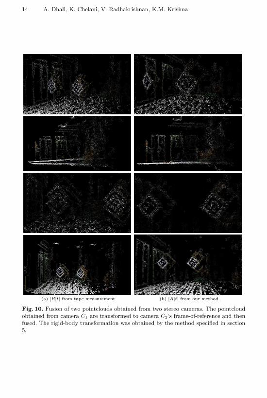
(a) [R|t| from tape measurement (b) [R|t| from our method
Fig. 10. Fusion of two pointclouds obtained from two stereo cameras. The pointcloudobtained from camera C1 are transformed to camera C2’s frame-of-reference and thenfused. The rigid-body transformation was obtained by the method specified in section5.
LiDAR-Camera Calibration using 3D-3D Point correspondences 15
To do this, we introduced the LiDAR which has a 360-degree field-of-viewand very precise 3D point co-ordinates can be obtained with it. We use it tofind transformations between the cameras. Once, this is done, we can removethe LiDAR; effectively using the LiDAR only for calibrating the cameras.
It is to be noted that the method described in this document calibrates amonocular camera and a LiDAR. If there is a stereo camera, we only calibratethe left camera and the LiDAR. Since, the baseline and stereo camera calibrationparameters are already known, calibrating only one of the cameras (left in ourcase) is sufficient to fuse the point clouds.
If we can find a transformation between two cameras C1 and C2, we caneasily extend the same procedure to obtain transformation between arbitrarynumber of cameras. Given, two (stereo) cameras, the proposed pipeline finds thetransformation that transforms all points in the LiDAR frame to the cameraframe.
We first run the algorithm, with C1 and LiDAR, L, and obtain a 4×4 matrix,
TLiDAR−to−C1(25)
We then run the algorithm, with C2 and LiDAR, L, and obtain a 4×4 matrix,
TLiDAR−to−C2(26)
Now, to obtain a transform that transforms all points in C1 to C2, we chainthe transforms, TLiDAR−to−C1 and TLiDAR−to−C2 ,
TC2−to−C1 = TLiDAR−to−C1 · T−1LiDAR−to−C2
= TLiDAR−to−C1 · TC2−to−LiDAR
(27)
Equation 27, finds the transform between C2 to C1, and if these are stereocameras, we can obtain point clouds and fuse them using this transform. If thetransform is very accurate, the two point clouds (from the two stereo cameras)will align properly. However, if there is translation error, when viewing the fusedpoint cloud, hallucinations of objects will be clearly visible, and there will betwo of everything. If there is error in the rotation, the points in the two cloudswill diverge more and more as the distance from the origin increases.
To verify the method in a more intuitive manner, lidar camera calibrationwas used to fuse point clouds obtained from two stereo cameras. We also providethe visualization of the fused point clouds.
5.1 Manual measurement vs. lidar camera calibration
First, we compare the calibration parameters obtained from our method againstmeticulously measured values using tape by a human.
The fused point cloud obtained when using manual measurements versuswhen using the method proposed in this document is shown in the video. Notice
16 A. Dhall, K. Chelani, V. Radhakrishnan, K.M. Krishna
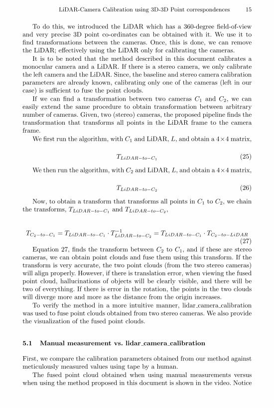
Fig. 11. Experimental setup for comparing point cloud fusing when using manualmeasurement versus using transformation obtained from lidar camera calibration.
the large translation error, even when the two cameras are kept on a planar sur-face. Hallucinations of markers, cupboards and carton box (in the background)can be seen as a result of the two point clouds not being aligned properly.
On the other hand, rotation and translation estimated by our package almostperfectly fuses the two individual point clouds. There is a very minute translationerror (1-2cm) and almost no rotation error. The fused point cloud is aligned soproperly, that one might actually believe that it is a single point cloud, but itactually consists of 2 clouds fused using extrinsic transformation between theirsources (the stereo cameras).
The resultant fused point clouds from both manual and lidar camera calibrationmethods can be seen on https://youtu.be/AbjRDtHLdz0.
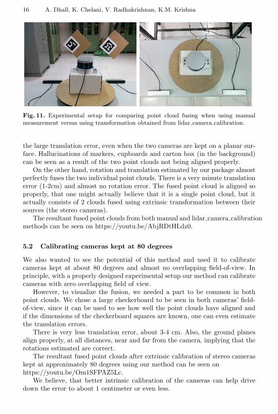
5.2 Calibrating cameras kept at 80 degrees
We also wanted to see the potential of this method and used it to calibratecameras kept at about 80 degrees and almost no overlapping field-of-view. Inprinciple, with a properly designed experimental setup our method can calibratecameras with zero overlapping field of view.
However, to visualize the fusion, we needed a part to be common in bothpoint clouds. We chose a large checkerboard to be seen in both cameras’ field-of-view, since it can be used to see how well the point clouds have aligned andif the dimensions of the checkerboard squares are known, one can even estimatethe translation errors.
There is very less translation error, about 3-4 cm. Also, the ground planesalign properly, at all distances, near and far from the camera, implying that therotations estimated are correct.
The resultant fused point clouds after extrinsic calibration of stereo cameraskept at approximately 80 degrees using our method can be seen onhttps://youtu.be/Om1SFPAZ5Lc.
We believe, that better intrinsic calibration of the cameras can help drivedown the error to about 1 centimeter or even less.
LiDAR-Camera Calibration using 3D-3D Point correspondences 17
Fig. 12. Experimental setup with cameras kept at about 80 degrees. The calibrationfor such configuration shows that our unique method can be, in principle, used forextrinsically calibrating cameras with no field-of-view overlap.
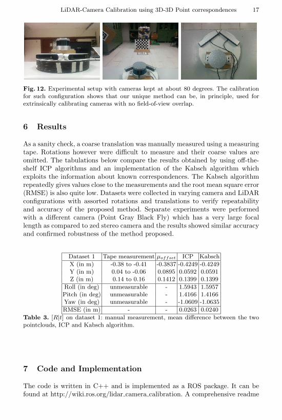
6 Results
As a sanity check, a coarse translation was manually measured using a measuringtape. Rotations however were difficult to measure and their coarse values areomitted. The tabulations below compare the results obtained by using off-the-shelf ICP algorithms and an implementation of the Kabsch algorithm whichexploits the information about known correspondences. The Kabsch algorithmrepeatedly gives values close to the measurements and the root mean square error(RMSE) is also quite low. Datasets were collected in varying camera and LiDARconfigurations with assorted rotations and translations to verify repeatabilityand accuracy of the proposed method. Separate experiments were performedwith a different camera (Point Gray Black Fly) which has a very large focallength as compared to zed stereo camera and the results showed similar accuracyand confirmed robustness of the method proposed.
Dataset 1 Tape measurement µoffset ICP Kabsch
X (in m) -0.38 to -0.41 -0.3837 -0.4249 -0.4249Y (in m) 0.04 to -0.06 0.0895 0.0592 0.0591Z (in m) 0.14 to 0.16 0.1412 0.1399 0.1399
Roll (in deg) unmeasurable - 1.5943 1.5957Pitch (in deg) unmeasurable - 1.4166 1.4166Yaw (in deg) unmeasurable - -1.0609 -1.0635
RMSE (in m) - - 0.0263 0.0240
Table 3. [R|t] on dataset 1: manual measurement, mean difference between the twopointclouds, ICP and Kabsch algorithm.
7 Code and Implementation
The code is written in C++ and is implemented as a ROS package. It can befound at http://wiki.ros.org/lidar camera calibration. A comprehensive readme
18 A. Dhall, K. Chelani, V. Radhakrishnan, K.M. Krishna
Dataset 2 Tape measurement µoffset ICP Kabsch
X (in m) -0.29 to -0.31 -0.2725 -0.3126 -0.3126Y (in m) -0.25 to -0.27 -0.0188 -0.2366 -0.2367Z (in m) 0.09 to -0.11 0.1152 0.1195 0.1196
Roll (in deg) unmeasurable - -0.3313 -0.3326Pitch (in deg) unmeasurable - 1.6615 1.6625Yaw (in deg) unmeasurable - -9.1813 -9.1854
RMSE (in m) - - 0.0181 0.0225
Table 4. [R|t] on dataset 2: manual measurement, mean difference between the twopointclouds, ICP and Kabsch algorithm.
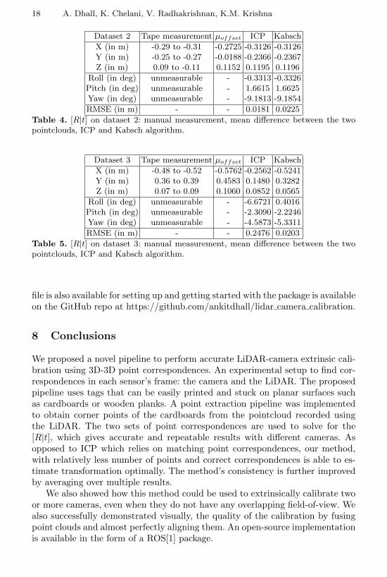
Dataset 3 Tape measurement µoffset ICP Kabsch
X (in m) -0.48 to -0.52 -0.5762 -0.2562 -0.5241Y (in m) 0.36 to 0.39 0.4583 0.1480 0.3282Z (in m) 0.07 to 0.09 0.1060 0.0852 0.0565
Roll (in deg) unmeasurable - -6.6721 0.4016Pitch (in deg) unmeasurable - -2.3090 -2.2246Yaw (in deg) unmeasurable - -4.5873 -5.3311
RMSE (in m) - - 0.2476 0.0203
Table 5. [R|t] on dataset 3: manual measurement, mean difference between the twopointclouds, ICP and Kabsch algorithm.
file is also available for setting up and getting started with the package is availableon the GitHub repo at https://github.com/ankitdhall/lidar camera calibration.
8 Conclusions
We proposed a novel pipeline to perform accurate LiDAR-camera extrinsic cali-bration using 3D-3D point correspondences. An experimental setup to find cor-respondences in each sensor’s frame: the camera and the LiDAR. The proposedpipeline uses tags that can be easily printed and stuck on planar surfaces suchas cardboards or wooden planks. A point extraction pipeline was implementedto obtain corner points of the cardboards from the pointcloud recorded usingthe LiDAR. The two sets of point correspondences are used to solve for the[R|t], which gives accurate and repeatable results with different cameras. Asopposed to ICP which relies on matching point correspondences, our method,with relatively less number of points and correct correspondences is able to es-timate transformation optimally. The method’s consistency is further improvedby averaging over multiple results.
We also showed how this method could be used to extrinsically calibrate twoor more cameras, even when they do not have any overlapping field-of-view. Wealso successfully demonstrated visually, the quality of the calibration by fusingpoint clouds and almost perfectly aligning them. An open-source implementationis available in the form of a ROS[1] package.

LiDAR-Camera Calibration using 3D-3D Point correspondences 19
References
1. Robot Operating System(ROS). http://www.ros.org/ 182. Martin Velas, Michal Spanel, Zdenek Materna, Adam Herout Calibration of RGB
Camera With Velodyne LiDAR. https://www.github.com/robofit/but velodyne/2, 8
3. Velodyne LiDAR. https://velodynelidar.com/ 94. ZED Stereo Camera. https://www.stereolabs.com/ 95. ArUco Markers. https://github.com/SmartRoboticSystems/aruco mapping
http://docs.opencv.org/3.1.0/d5/dae/tutorial aruco detection.html 8, 96. V. Lepetit and F.Moreno-Noguer and P.Fua EPnP: An Accurate O(n) Solution to
the PnP Problem. International Journal Computer Vision, 2009 57. April Tags. https://april.eecs.umich.edu/wiki/AprilTags 88. Iterative Closest Point. https://en.wikipedia.org/wiki/Iterative closest point 109. Olga Sorkine-Hornung and Michael Rabinovich Least-Squares Rigid Motion Using
SVD. https://igl.ethz.ch/projects/ARAP/svd rot.pdf 1010. Lydia E. Kavraki Molecular Distance Measures. http://cnx.org/contents/HV-
RsdwL@23/Molecular-Distance-Measures 10