LIDAR-based 3D Object Perception

M. Himmelsbach, A. Muller, T. Luttel and H.-J. Wunsche

Abstract— This paper describes a LIDAR-based perceptionsystem for ground robot mobility, consisting of 3D objectdetection, classification and tracking. The presented systemwas demonstrated on-board our autonomous ground vehicleMuCAR-3, enabling it to safely navigate in urban traffic-likescenarios as well as in off-road convoy scenarios. The efficiencyof our approach stems from the unique combination of 2D and3D data processing techniques. Whereas fast segmentation ofpoint clouds into objects is done in a 2 1

2D occupancy grid,

classifying the objects is done on raw 3D point clouds. Forfast switching of domains, the occupancy grid is enhanced toact like a hash table for retrieval of 3D points. In contrast tomost existing work on 3D point cloud classification, where real-time operation is often impossible, this combination allows oursystem to perform in real-time at 0.1s frame-rate.

I. INTRODUCTION

In this paper we address the problem of segmenting 3Dscan data into objects of known classes. Given the set ofpoints in 3D acquired by a range scanner, the goal ofsegmentation is to attribute the points to a set of candidateobject classes. In the context of ground robot mobility, thissegmentation capability is not only essential for high-leveltasks like scene understanding and planning, but can alsobe used for scan registration and robot localization, e.g. in aSLAM framework [1]. Besides, knowing the object’s class isespecially useful in dynamic environments, both for planningand estimation: estimation can be improved by making useof appropriate dynamic models, and planning can incorporateknowledge about the behavior or intentions typical of acertain object class.

Our approach to perception is decomposed into three mainsteps: segmentation, classification and tracking. The segmen-tation step is performed on an occupancy grid, yielding con-nected components of grid cells not belonging to the groundsurface. In an efficient operation, we determine all the 3DLIDAR point measurements corresponding to the segmentedobjects. In the classification step, we extract features froman object’s point cloud, capturing the distribution of localspatial and reflectivity properties extracted over a fixed-sizesupport volume around each point. In a supervised learningframework, a support vector machine (SVM) classifier istrained to discriminate the classes of interest, e.g. other trafficparticipants in our case, given hand-labeled examples ofpoint clouds.

The method is not restricted to a particular robot or sensor,however we describe and demonstrate it using our vehicle

This work was supported by COTESYS cluster of excellence.All authors are with department of Aerospace Engineering, Autonomous

Systems Technology (TAS), University of the Bundeswehr Munich, Neu-biberg, Germany.

Contact author email: michael.himmelsbach@unibw.de

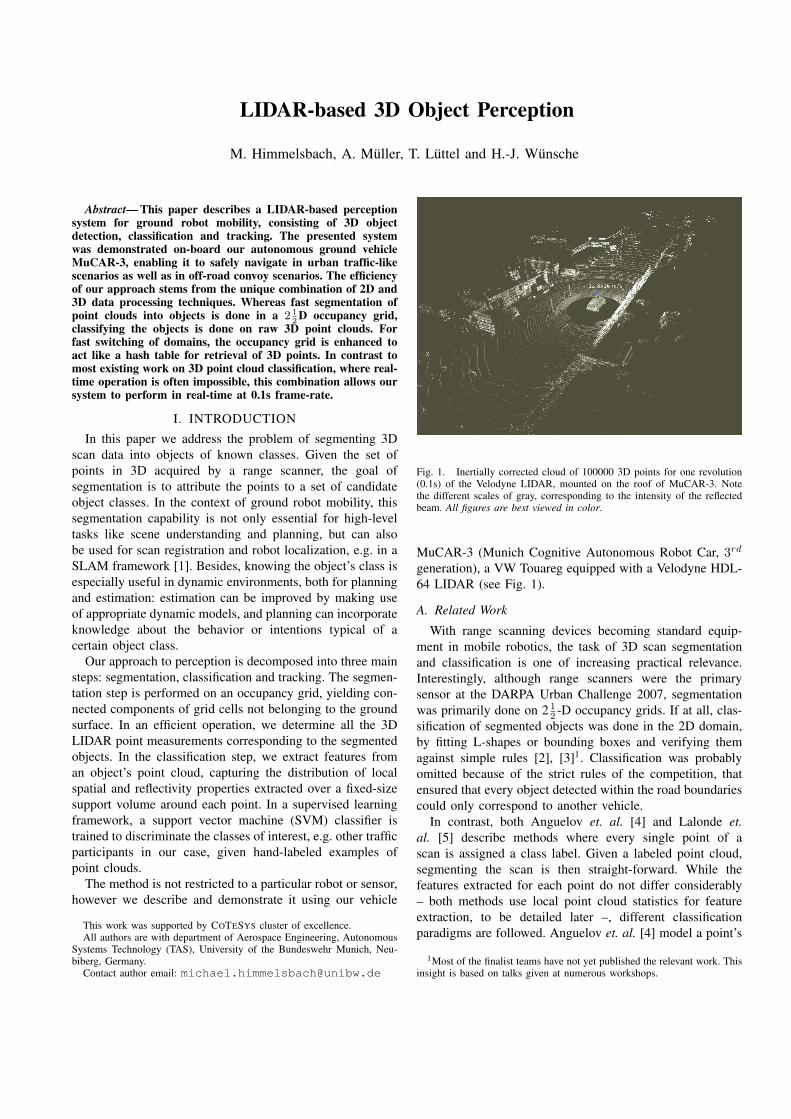
Fig. 1. Inertially corrected cloud of 100000 3D points for one revolution(0.1s) of the Velodyne LIDAR, mounted on the roof of MuCAR-3. Notethe different scales of gray, corresponding to the intensity of the reflectedbeam. All figures are best viewed in color.

MuCAR-3 (Munich Cognitive Autonomous Robot Car, 3rd

generation), a VW Touareg equipped with a Velodyne HDL-64 LIDAR (see Fig. 1).

A. Related Work

With range scanning devices becoming standard equip-ment in mobile robotics, the task of 3D scan segmentationand classification is one of increasing practical relevance.Interestingly, although range scanners were the primarysensor at the DARPA Urban Challenge 2007, segmentationwas primarily done on 2 1

2 -D occupancy grids. If at all, clas-sification of segmented objects was done in the 2D domain,by fitting L-shapes or bounding boxes and verifying themagainst simple rules [2], [3]1. Classification was probablyomitted because of the strict rules of the competition, thatensured that every object detected within the road boundariescould only correspond to another vehicle.

In contrast, both Anguelov et. al. [4] and Lalonde et.al. [5] describe methods where every single point of ascan is assigned a class label. Given a labeled point cloud,segmenting the scan is then straight-forward. While thefeatures extracted for each point do not differ considerably– both methods use local point cloud statistics for featureextraction, to be detailed later –, different classificationparadigms are followed. Anguelov et. al. [4] model a point’s

1Most of the finalist teams have not yet published the relevant work. Thisinsight is based on talks given at numerous workshops.

class label by a probability distribution conditioned on thelocal features and the labels in the point’s neighborhood.They thus enforce spatial contiguity, exploiting the fact thatadjacent points in the scan should have similar labels. Thisdistribution is modeled by a Markov Random Field (MRF),whose parameters are determined in a supervised learningstage such that the resulting classifier maximizes the marginbetween the classes learned, like SVMs do. Although notiming results are given in [4], it can be concluded from [6]that the method does not permit real-time use.

Lalonde et.al. [5] learn a parametric model of the featuredistribution for each class by fitting a Gaussian mixturemodel (GMM) using the Expectation Maximization (EM)algorithm on a hand labeled training data set. Spatial con-tiguity is accounted for by running simple rule-based filtersafter classification, e.g. by changing a point’s label to themost frequent class among its neighbors. However, to maketheir method perform in real-time, some modifications arenecessary. Especially, they no longer classify individualpoints, but an artificial prototype point of all points containedin a 3D voxel grid cell, such that 7000 voxels/sec. can beclassified.

We take a quite different, unique approach to objectclassification in 3D point clouds, in that segmentation isbased on the compressed data contained in a 2 1

2 D occupancygrid. We then make use of the rich information containedin the Velodyne’s 3D point clouds by again switching thedomain to 3D, now classifying only subsets of the scan’stotal point cloud, with evidence that each subset represents anindividual object. Thanks to the efficient combination of 2Dand 3D data processing techniques, classification of objectsrepresented by their 3D point clouds is possible in real-timeon-board an autonomous vehicle.

II. OBJECT DETECTIONA. Occupancy Grid

We use a 2 12 -D ego-centered occupancy grid of dimension

100m×100m, each cell covering a small ground patch of0.15m×0.15m. Each cell stores a single value expressing thedegree of how occupied that cell is by an obstacle. In ourimplementation this value is a metric length with the physicalunit [m]. Before we detail its meaning and calculation, notethat in our approach we create a new occupancy grid oneach new LIDAR revolution, i.e. every 0.1s. Thus, we donot accumulate data for a longer time. The reasons for thisdecision are twofold. First, one revolution of the Velodynesupplies about 100000 3D points, which proved to be suffi-cient. Second, the quality of an accumulated occupancy gridcan easily deteriorate if the physical movement of the sensoris not estimated with very high precision. Small angulardeviations in the estimate of the sensor’s pose can resultin large errors. Registering scans against each other, e.g.using the ICP algorithm [7] or some of its derivatives, couldsolve this problem, but would require substantial additionalcomputational load.

For calculating the occupancy values, we first inertiallycorrect the LIDAR scan, taking the vehicle’s motion into

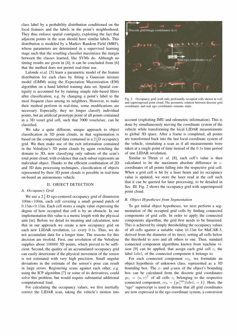
Fig. 2. Occupancy grid (with only profoundly occupied cells shown in red)and superimposed point cloud. The geometric relation between discrete gridcoordinates and real ego coordinates remains static.

account (exploiting IMU and odometric information). This isdone by simultaneously moving the coordinate system of thevehicle while transforming the local LIDAR measurementsto global 3D space. After a frame is completed, all pointsare transformed back into the last local coordinate system ofthe vehicle, simulating a scan as if all measurements weretaken at a single point of time instead of the 0.1s time periodof one LIDAR revolution.

Similar to Thrun et. al. [8], each cell’s value is thencalculated to be the maximum absolute difference in z-coordinates of all points falling into the respective grid cell.When a grid cell is hit by a laser beam and its occupancyvalue is updated, we store the laser read at the cell suchthat it can be queried for later processing, to be detailed inSec. III. Fig. 2 shows the occupancy grid with superimposedpoint cloud.

B. Object Hypotheses from Segmentation

To get initial object hypotheses, we next perform a seg-mentation of the occupied grid cells by finding connectedcomponents of grid cells. In order to apply the connectedcomponents algorithm, the grid first needs to be binarized.This is achieved by simply thresholding the occupancy valuesof all cells against a suitable value (0.15m for MuCAR-3,derived from the diameter of its tires), setting all cells belowthe threshold to zero and all others to one. Then, standardconnected component algorithms known from machine vi-sion [9] can be applied, that assign each grid cell ci thelabel labeli of the connected component it belongs to.

For each connected component cck, we formulate anobject hypothesis of unknown class, represented as a 3Dbounding box. The x- and y-axis of the object’s boundingbox can be calculated from the discrete grid coordinatesgci = (u, v)T of all cells ci belonging to the respectiveconnected component, cck = {gcego

i |labeli = k}. Here, the“ego” superscript is used to denote that all grid coordinatesare now expressed in the ego coordinate system, a conversion

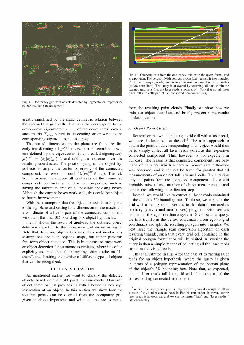
Fig. 3. Occupancy grid with objects detected by segmentation, representedby 3D bounding boxes (green).

greatly simplified by the static geometric relation betweenthe ego and the grid cells. The axes then correspond to theorthonormal eigenvectors e1, e2 of the coordinates’ covari-ance matrix Σcck

, sorted in descending order w.r.t. to thecorresponding eigenvalues, i.e. d1 ≥ d2.

The boxes’ dimensions in the plane are found by lin-early transforming all gcego

i ∈ cck into the coordinate sys-tem defined by the eigenvectors (the so-called eigenspace),gcego∗

i = (e1|e2)gcegoi , and taking the extremes over the

resulting coordinates. The position posk of the object hy-pothesis is simply the center of gravity of the connectedcomponent, i.e. posk = |cck|−1Σ(gcego

i ∈ cck). This 2Dbox is assured to enclose all grid cells of the connectedcomponent, but lacks some desirable properties, such ashaving the minimum area of all possible enclosing boxes.Although the current boxes work well, this could be subjectto future improvement.

With the assumption that the object’s z-axis is orthogonalto the xy-plane and setting its z-dimension to the maximumz-coordinate of all cells part of the connected component,we obtain the final 3D bounding box object hypothesis.

Fig. 3 shows the result of applying the outlined objectdetection algorithm to the occupancy grid shown in Fig. 2.Note that detecting objects this way does not involve anyassumptions about an object’s shape, but rather performsfree-form object detection. This is in contrast to most workon object detection for autonomous vehicles, where it is oftenexplicitly assumed that all interesting objects take on “L-shape”, thus limiting the number of different types of objectsthat can be recognized.

III. CLASSIFICATION

As mentioned earlier, we want to classify the detectedobjects based on their 3D point measurements. However,object detection just provides us with a bounding box rep-resentation of an object. In this section we show how therequired points can be queried from the occupancy gridgiven an object hypothesis and what features are extracted

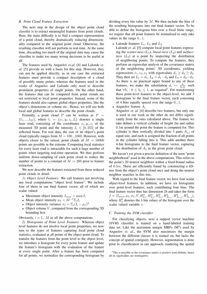
Fig. 4. Querying data from the occupancy grid, with the query formulatedas a polygon. The polygon (with vertices shown blue) gets split into triangles(2 in this example, white) and scan conversion is issued on all triangles(yellow scan lines). The query is answered by returning all data within thescanned grid cells (i.e. the laser reads, shown grey). Note that not all laserreads fall into cells part of the connected component (red).

from the resulting point clouds. Finally, we show how wetrain our object classifiers and briefly present some resultsof classification.

A. Object Point Clouds

Remember that when updating a grid cell with a laser read,we store the laser read at the cell2. The naive approach toobtain the point cloud corresponding to an object would thusbe to simply collect all laser reads stored at the respectiveconnected component. This, however, is not expedient inour case. The reason is that connected components are onlymade of cells for which a certain z-coordinate differencewas observed, and it can not be taken for granted that allmeasurements of an object fall into such cells. Thus, takingonly the points from the connected component cells wouldprobably miss a large number of object measurements andharden the following classification step.

Instead, we would like to extract all laser reads containedin the object’s 3D bounding box. To do so, we augment thegrid with a facility to answer queries for data formulated asarbitrary (convex and non-convex) polygons, with verticesdefined in the ego coordinate system. Given such a query,we first transform the vertex coordinates from ego to gridcoordinates and split the resulting polygon into triangles. Wenext issue the triangle scan conversion algorithm on eachresulting triangle, such that every grid cell contained in theoriginal polygon formulation will be visited. Answering thequery is then a simple matter of collecting all the laser readsstored at the visited cells.

This is illustrated in Fig. 4 for the case of extracting laserreads for an object hypothesis, where the query is givenin terms of a polygon representation of the bottom planeof the object’s 3D bounding box. Note that, as expected,not all laser reads fall into grid cells that are part of thecorresponding connected component.

2In fact, the occupancy grid is implemented general enough to allowstorage of any kind of data at the cells. For this application, however, storinglaser reads is appropriate, and we use the terms “data” and “laser read(s)”interchangeably.

B. Point Cloud Feature Extraction

The next step in the design of the object point cloudclassifer is to extract meaningful features from point clouds.Here, the main difficulty is to find a compact representationof a point cloud, thereby dramatically reducing dimension-ality compared to the original point cloud. Otherwise, theresulting classifier will not perform in real-time. At the sametime, discarding too much of the original data may cause theclassifier to make too many wrong decisions to be useful atall.

The features used by Anguelov et.al. [4] and Lalonde et.al. [5] provide us with a basis for this step. However, theycan not be applied directly, as in our case the extractedfeatures must provide a compact description of a cloudof possibly many points, whereas the features used in theworks of Anguelov and Lalonde only need to describeprominent properties of single points. On the other hand,the features that can be computed from point clouds arenot restricted to local point properties. Instead, some of thefeatures should also capture global object properties, like theobject’s dimensions or volume etc.. Hence, we will use bothlocal and global features to describe the point clouds.

Formally, a point cloud P can be written as P ={l1, ..., lM}, where li = {xi, yi, zi, Ii} denotes a singlelaser read, consisting of the coordinates xi, yi, zi of themeasured 3D point and the intensity Ii ∈ [0, 255] of thereflected beam. For real data, the size of an object’s pointcloud typically ranges from M = 100...1000. However, withobjects closer to the sensor, point clouds of M = 10000points are possible in the extreme. Computing local statisticsfor every laser read is intractable for such a large number ofpoints when targeting real-time operation. We thus performuniform down-sampling of each point cloud to reduce thenumber of points to a constant of M := 200 prior to featureextraction.

We now describe the features extracted from these reducedpoint clouds in detail.

1) Object Level Features: We call features not involvingany local computations “object level feature”. We includefour of them in our final feature vector, all of which arescalar valued.• Maximum object intensity Imax = max Ii• Mean object intensity µI = M−1ΣiIi• Object intensity variance σI = Σi(Ii − µI)2

• Object volume V , computed from the corresponding 3Dbounding box

Obviously, i = 1...M in all the above computations.2) Histograms of Point Level Features: Whereas object

level features do not involve local point properties, we nowturn to the types of features capturing local point cloudstatistics, evaluated at all points of the object point cloud. Totransfer the features from the point level to the object level,we introduce a histogram for every point feature and updatethe feature’s histogram with the evaluation of the featureat every single point. After a feature has been computedfor all points, we normalize the corresponding histogram by

dividing every bin value by M . We then include the bins ofthe resulting histograms into our final feature vector. To beable to define the histogram bins over a fixed finite range,we require that all point features be normalized to only takevalues in the range 0...1.

• Lalonde features L1, L2 and L3

Lalonde et. al. [5] compute local point features express-ing the scatter-ness (L1), linear-ness (L2) and surface-ness (L3) at a point by inspecting the distributionof neighboring points. To compute the features, theyperform an eigenvalue analysis of the covariance matrixof the neighboring points’ 3D coordinates, yieldingeigenvectors e1, e2, e3 with eigenvalues d1 ≥ d2 ≥ d3.They then set L1 = d1, L2 = d1−d2 and L3 = d2−d3.As there is no practical upper bound to any of thesefeatures, we make the substitution di 7→ di

Σidisuch

that ∀hi : 0 ≤ hi ≤ 1, as required3. For transformingthese point-level features to the object-level, we add 3histograms to the final feature vector, each consistingof 4 bins equally spaced over the range 0...1.

• Anguelov feature A1

Anguelov et. al. [4] describe two features, but only oneis used in our work as the other do not differ signifi-cantly from the ones calculated above. The feature wetake defines a vertical cylinder of height 2m and radius0.1m around the point the feature is computed for. Thiscylinder is then vertically divided into 3 parts A1,i ofequal size, and each is assigned the fraction of all pointsin the cylinder falling into it. This adds another three4-bin histograms to the final feature vector, capturingthe distribution of A1 in the given point cloud.

We haven’t yet given a precise definition of the term “pointneighborhood” used in the above computations. This refers tothe point’s 20 nearest neighbors within a fixed-bound radiusof 0.5m. These are efficiently found by constructing a kD-tree from the object’s point cloud once and doing the nearestneighbor searches in this tree.

With regard to the final feature vector, we have four scalarobject-level features. In addition, we have six histogramsover point-level features, each contributing four bins. Thefinal feature vector thus has dimension 28 and takes the formf = (Imax, µI , σI , V,H

4L1, H4

L2, H4

L3, H4

A1,1, H4

A1,2, H4

A1,3),

where Hbv denotes the b bin values of the histogram over the

scalar valued variable v.

C. Training the SVM classifier

For classifying objects, next a support vector machine(SVM) classifier is trained on a hand-labeled trainingdata set. Like the maximum margin MRFs (M3) used byAnguelov et. al., the SVM also maximizes the marginbetween the different classes it is trained on, but lacks theconcept of spatial contiguity. However, segmentation is doneprior to classification in our approach, rendering the spatial

3This is possible as the covariance matrix is positive semi-definite, henceall its eigenvalues are nonnegative.

contiguity property less important. We use the common ν-SVM variant, that allows for some mislabeled examples incase the classes are not completely separable in feature space[10]. The approach taken to multi-class classification is thatof one-against-all classification, where one binary SVM istrained for every class, separating it from all other classes.

The operation of the ν-SVM depends on two parameters:C is a penalty parameter for weighting classification errorsand γ is a kernel function parameter. To also determinethe optimal choice of these parameters, we perform a grid-search in a suitable subspace of parameter values. At eachgrid resolution, the classification performance for differentpairings of C, γ, given by the grid cells, is evaluated byrandomly splitting the training data set into two folds of equalsize. Applying the concept of cross-validation, one fold isthen used for training the SVM using the current parameterchoices and the other fold for evaluation. The search theniterates by refining the resolution of the grid and centeringit at the best parameter choices of the last iteration.

D. Two-class Classification Results

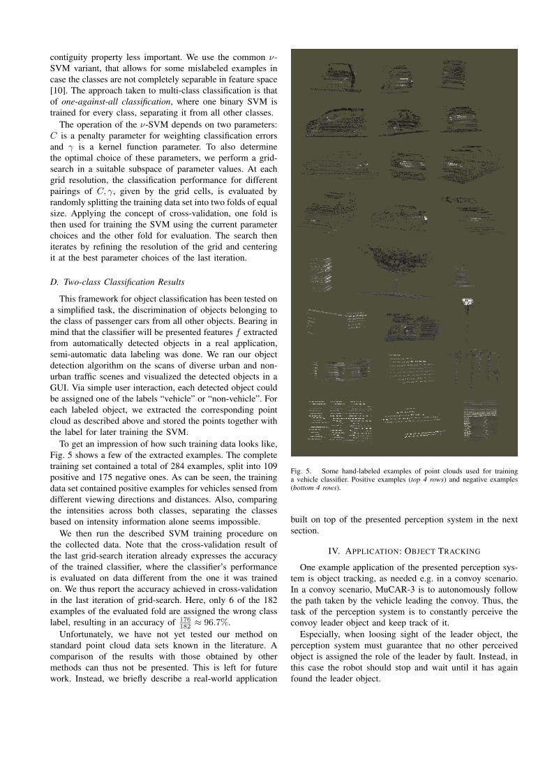
This framework for object classification has been tested ona simplified task, the discrimination of objects belonging tothe class of passenger cars from all other objects. Bearing inmind that the classifier will be presented features f extractedfrom automatically detected objects in a real application,semi-automatic data labeling was done. We ran our objectdetection algorithm on the scans of diverse urban and non-urban traffic scenes and visualized the detected objects in aGUI. Via simple user interaction, each detected object couldbe assigned one of the labels “vehicle” or “non-vehicle”. Foreach labeled object, we extracted the corresponding pointcloud as described above and stored the points together withthe label for later training the SVM.

To get an impression of how such training data looks like,Fig. 5 shows a few of the extracted examples. The completetraining set contained a total of 284 examples, split into 109positive and 175 negative ones. As can be seen, the trainingdata set contained positive examples for vehicles sensed fromdifferent viewing directions and distances. Also, comparingthe intensities across both classes, separating the classesbased on intensity information alone seems impossible.

We then run the described SVM training procedure onthe collected data. Note that the cross-validation result ofthe last grid-search iteration already expresses the accuracyof the trained classifier, where the classifier’s performanceis evaluated on data different from the one it was trainedon. We thus report the accuracy achieved in cross-validationin the last iteration of grid-search. Here, only 6 of the 182examples of the evaluated fold are assigned the wrong classlabel, resulting in an accuracy of 176

182 ≈ 96.7%.Unfortunately, we have not yet tested our method on

standard point cloud data sets known in the literature. Acomparison of the results with those obtained by othermethods can thus not be presented. This is left for futurework. Instead, we briefly describe a real-world application

Fig. 5. Some hand-labeled examples of point clouds used for traininga vehicle classifier. Positive examples (top 4 rows) and negative examples(bottom 4 rows).

built on top of the presented perception system in the nextsection.

IV. APPLICATION: OBJECT TRACKING

One example application of the presented perception sys-tem is object tracking, as needed e.g. in a convoy scenario.In a convoy scenario, MuCAR-3 is to autonomously followthe path taken by the vehicle leading the convoy. Thus, thetask of the perception system is to constantly perceive theconvoy leader object and keep track of it.

Especially, when loosing sight of the leader object, theperception system must guarantee that no other perceivedobject is assigned the role of the leader by fault. Instead, inthis case the robot should stop and wait until it has againfound the leader object.

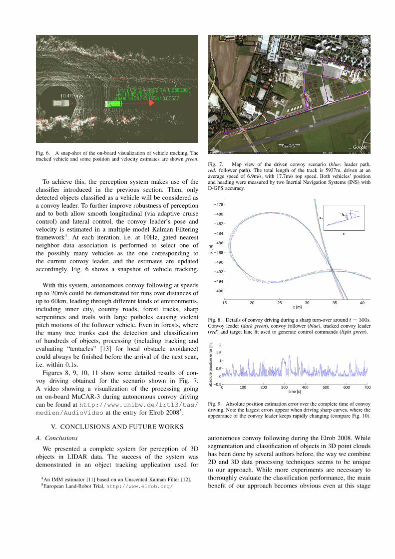
Fig. 6. A snap-shot of the on-board visualization of vehicle tracking. Thetracked vehicle and some position and velocity estimates are shown green.

To achieve this, the perception system makes use of theclassifier introduced in the previous section. Then, onlydetected objects classified as a vehicle will be considered asa convoy leader. To further improve robustness of perceptionand to both allow smooth longitudinal (via adaptive cruisecontrol) and lateral control, the convoy leader’s pose andvelocity is estimated in a multiple model Kalman Filteringframework4. At each iteration, i.e. at 10Hz, gated nearestneighbor data association is performed to select one ofthe possibly many vehicles as the one corresponding tothe current convoy leader, and the estimates are updatedaccordingly. Fig. 6 shows a snapshot of vehicle tracking.

With this system, autonomous convoy following at speedsup to 20m/s could be demonstrated for runs over distances ofup to 60km, leading through different kinds of environments,including inner city, country roads, forest tracks, sharpserpentines and trails with large potholes causing violentpitch motions of the follower vehicle. Even in forests, wherethe many tree trunks cast the detection and classificationof hundreds of objects, processing (including tracking andevaluating “tentacles” [13] for local obstacle avoidance)could always be finished before the arrival of the next scan,i.e. within 0.1s.

Figures 8, 9, 10, 11 show some detailed results of con-voy driving obtained for the scenario shown in Fig. 7.A video showing a visualization of the processing goingon on-board MuCAR-3 during autonomous convoy drivingcan be found at http://www.unibw.de/lrt13/tas/medien/AudioVideo at the entry for Elrob 20085.

V. CONCLUSIONS AND FUTURE WORKS

A. Conclusions

We presented a complete system for perception of 3Dobjects in LIDAR data. The success of the system wasdemonstrated in an object tracking application used for

4An IMM estimator [11] based on an Unscented Kalman Filter [12].5European Land-Robot Trial, http://www.elrob.org/

Fig. 7. Map view of the driven convoy scenario (blue: leader path,red: follower path). The total length of the track is 5937m, driven at anaverage speed of 6.9m/s, with 17.7m/s top speed. Both vehicles’ positionand heading were measured by two Inertial Navigation Systems (INS) withD-GPS accuracy.

15 20 25 30 35 40

−496

−494

−492

−490

−488

−486

−484

−482

−480

−478

x [m]

y [m

]

x

yFig. 8. Details of convoy driving during a sharp turn-over around t = 300s.Convoy leader (dark green), convoy follower (blue), tracked convoy leader(red) and target lane fit used to generate control commands (light green).

0 100 200 300 400 500 600 700−0.5

0

0.5

1

1.5

2

time [s]

abso

lute

pos

ition

err

or [m

]

Fig. 9. Absolute position estimation error over the complete time of convoydriving. Note the largest errors appear when driving sharp curves, where theappearance of the convoy leader keeps rapidly changing (compare Fig. 10).

autonomous convoy following during the Elrob 2008. Whilesegmentation and classification of objects in 3D point cloudshas been done by several authors before, the way we combine2D and 3D data processing techniques seems to be uniqueto our approach. While more experiments are necessary tothoroughly evaluate the classification performance, the mainbenefit of our approach becomes obvious even at this stage

0 100 200 300 400 500 600 700−2

−1

0

1

2

time [s]

rela

tive

head

ing

[rad

]

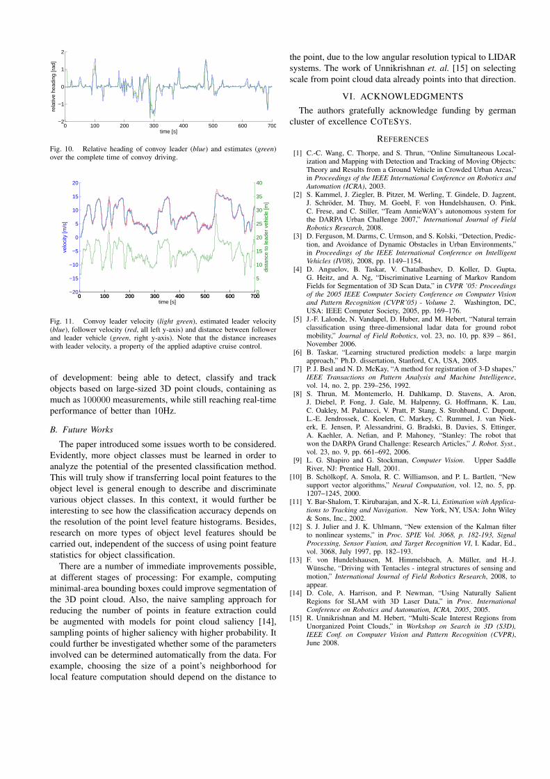
Fig. 10. Relative heading of convoy leader (blue) and estimates (green)over the complete time of convoy driving.

0 100 200 300 400 500 600 700−20

−15

−10

−5

0

5

10

15

20

time [s]

velo

city

[m/s

]

0 100 200 300 400 500 600 7000

5

10

15

20

25

30

35

40

dist

ance

to le

ader

veh

icle

[m]

Fig. 11. Convoy leader velocity (light green), estimated leader velocity(blue), follower velocity (red, all left y-axis) and distance between followerand leader vehicle (green, right y-axis). Note that the distance increaseswith leader velocity, a property of the applied adaptive cruise control.

of development: being able to detect, classify and trackobjects based on large-sized 3D point clouds, containing asmuch as 100000 measurements, while still reaching real-timeperformance of better than 10Hz.

B. Future Works

The paper introduced some issues worth to be considered.Evidently, more object classes must be learned in order toanalyze the potential of the presented classification method.This will truly show if transferring local point features to theobject level is general enough to describe and discriminatevarious object classes. In this context, it would further beinteresting to see how the classification accuracy depends onthe resolution of the point level feature histograms. Besides,research on more types of object level features should becarried out, independent of the success of using point featurestatistics for object classification.

There are a number of immediate improvements possible,at different stages of processing: For example, computingminimal-area bounding boxes could improve segmentation ofthe 3D point cloud. Also, the naive sampling approach forreducing the number of points in feature extraction couldbe augmented with models for point cloud saliency [14],sampling points of higher saliency with higher probability. Itcould further be investigated whether some of the parametersinvolved can be determined automatically from the data. Forexample, choosing the size of a point’s neighborhood forlocal feature computation should depend on the distance to

the point, due to the low angular resolution typical to LIDARsystems. The work of Unnikrishnan et. al. [15] on selectingscale from point cloud data already points into that direction.

VI. ACKNOWLEDGMENTS

The authors gratefully acknowledge funding by germancluster of excellence COTESYS.

REFERENCES

[1] C.-C. Wang, C. Thorpe, and S. Thrun, “Online Simultaneous Local-ization and Mapping with Detection and Tracking of Moving Objects:Theory and Results from a Ground Vehicle in Crowded Urban Areas,”in Proceedings of the IEEE International Conference on Robotics andAutomation (ICRA), 2003.

[2] S. Kammel, J. Ziegler, B. Pitzer, M. Werling, T. Gindele, D. Jagzent,J. Schroder, M. Thuy, M. Goebl, F. von Hundelshausen, O. Pink,C. Frese, and C. Stiller, “Team AnnieWAY’s autonomous system forthe DARPA Urban Challenge 2007,” International Journal of FieldRobotics Research, 2008.

[3] D. Ferguson, M. Darms, C. Urmson, and S. Kolski, “Detection, Predic-tion, and Avoidance of Dynamic Obstacles in Urban Environments,”in Proceedings of the IEEE International Conference on IntelligentVehicles (IV08), 2008, pp. 1149–1154.

[4] D. Anguelov, B. Taskar, V. Chatalbashev, D. Koller, D. Gupta,G. Heitz, and A. Ng, “Discriminative Learning of Markov RandomFields for Segmentation of 3D Scan Data,” in CVPR ’05: Proceedingsof the 2005 IEEE Computer Society Conference on Computer Visionand Pattern Recognition (CVPR’05) - Volume 2. Washington, DC,USA: IEEE Computer Society, 2005, pp. 169–176.

[5] J.-F. Lalonde, N. Vandapel, D. Huber, and M. Hebert, “Natural terrainclassification using three-dimensional ladar data for ground robotmobility,” Journal of Field Robotics, vol. 23, no. 10, pp. 839 – 861,November 2006.

[6] B. Taskar, “Learning structured prediction models: a large marginapproach,” Ph.D. dissertation, Stanford, CA, USA, 2005.

[7] P. J. Besl and N. D. McKay, “A method for registration of 3-D shapes,”IEEE Transactions on Pattern Analysis and Machine Intelligence,vol. 14, no. 2, pp. 239–256, 1992.

[8] S. Thrun, M. Montemerlo, H. Dahlkamp, D. Stavens, A. Aron,J. Diebel, P. Fong, J. Gale, M. Halpenny, G. Hoffmann, K. Lau,C. Oakley, M. Palatucci, V. Pratt, P. Stang, S. Strohband, C. Dupont,L.-E. Jendrossek, C. Koelen, C. Markey, C. Rummel, J. van Niek-erk, E. Jensen, P. Alessandrini, G. Bradski, B. Davies, S. Ettinger,A. Kaehler, A. Nefian, and P. Mahoney, “Stanley: The robot thatwon the DARPA Grand Challenge: Research Articles,” J. Robot. Syst.,vol. 23, no. 9, pp. 661–692, 2006.

[9] L. G. Shapiro and G. Stockman, Computer Vision. Upper SaddleRiver, NJ: Prentice Hall, 2001.

[10] B. Scholkopf, A. Smola, R. C. Williamson, and P. L. Bartlett, “Newsupport vector algorithms,” Neural Computation, vol. 12, no. 5, pp.1207–1245, 2000.

[11] Y. Bar-Shalom, T. Kirubarajan, and X.-R. Li, Estimation with Applica-tions to Tracking and Navigation. New York, NY, USA: John Wiley& Sons, Inc., 2002.

[12] S. J. Julier and J. K. Uhlmann, “New extension of the Kalman filterto nonlinear systems,” in Proc. SPIE Vol. 3068, p. 182-193, SignalProcessing, Sensor Fusion, and Target Recognition VI, I. Kadar, Ed.,vol. 3068, July 1997, pp. 182–193.

[13] F. von Hundelshausen, M. Himmelsbach, A. Muller, and H.-J.Wunsche, “Driving with Tentacles - integral structures of sensing andmotion,” International Journal of Field Robotics Research, 2008, toappear.

[14] D. Cole, A. Harrison, and P. Newman, “Using Naturally SalientRegions for SLAM with 3D Laser Data,” in Proc. InternationalConference on Robotics and Automation, ICRA, 2005, 2005.

[15] R. Unnikrishnan and M. Hebert, “Multi-Scale Interest Regions fromUnorganized Point Clouds,” in Workshop on Search in 3D (S3D),IEEE Conf. on Computer Vision and Pattern Recognition (CVPR),June 2008.