LICOS Discussion Paper Series

Discussion Paper 319/2012

Biofuels and Food Security: Micro-evidence from Ethiopia

Martha Negash and Jo Swinnen

Katholieke Universiteit Leuven

LICOS Centre for Institutions and Economic Performance Waaistraat 6 – mailbox 3511 3000 Leuven BELGIUM TEL:+32-(0)16 32 65 98 FAX:+32-(0)16 32 65 99 http://www.econ.kuleuven.be/licos

Biofuels and Food Security:

Micro-evidence from Ethiopia

Martha Negash 1 and Johan Swinnen

1,2

1 LICOS Centre for Institutions and Economic Performance

& Department of Economics

Katholieke Universiteit Leuven

2 Centre for Food Security and the Environment (FSE)

Stanford University

Version: 17 September 2012

Abstract

This paper provides microeconomic evidence on food security impacts of privately

organized biofuel outgrower schemes in Ethiopia. We conducted a household and

community level survey and evaluated the impact of castor bean farming. We use

endogenous switching regressions to analyze the impact on food security. Food security

(as measured by a “food gap”) and food caloric intake is significantly better in households

producing castor beans. “Fuel” and “food” are complements rather than substitutes at the

micro-level in castor production in Ethiopia.

Keywords: biofuel, castor, food security, Ethiopia

JEL: Q42, Q16, O13, Q12

Corresponding author: Martha Negash, martha.negash@kuleuven.be

This research was financially supported by the KU Leuven Research Council (EF and

Methusalem projects). The authors acknowledge useful comments by conference and seminar

participants in Stanford, IAAE (Foz do Iguaçu, Brazil), ICABR (Ravello, Italy) and LICOS.

2

1. Introduction

Biofuel development is a controversial issue, in particular in developing countries.

Biofuels are said to cause environmental problems and to worsen food security – reflected in

the ‘food’ versus ‘fuel’ debate (Cotula et al., 2010; Pimentel et al., 2009; Bindraban et al.,

2009; Fargione et al., 2007). Some studies show that biofuel investments provide

alternative income through employment, boost economic growth and reduce the incidence

of poverty (Arndt et al., 2011; Huang et al., 2012; IIED, 2009). Others suggest that biofuel

expansion jeopardizes food security goals (IFPRI, 2008; Mitchell, 2008; FAO, 2008).

So far analyses of the impacts of biofuel development have been based on qualitative

case studies or on aggregate economy-wide simulation models or computable general

equilibrium (CGE) analyses. The later have focused on impacts on prices (Ajanovic, 2011;

Ciaian and Kancs, 2011), on income and GDP (Arndt, 2011; Ewing and Msangi, 2009) or the

world economy (Taheripour et al, 2009). There is no quantitative empirical evidence on the

actual impact of biofuels on the rural poor and smallholder farmers.

To fill the gap in our understanding, we estimate the effects of production contracts

between smallholder farmers and a biofuel company on farmers’ food security. We use

detailed company and survey data from Ethiopia. Ethiopia is an excellent case to study these

effects. On the one hand, Ethiopia is a major energy importer. In fact it is viewed as the

number one “energy poor country” in the world (Nussbaumer, et al, 2011)1. Developing

renewable alternative resources therefore sounds appealing. On the other hand, Ethiopia’s

agriculture sector is heavily dominated by subsistence smallholder farmers whose food

security is vulnerable and who are often food aid recipients (Devereux and Guenther, 2009).

It is therefore argued that expansion of biofuels may compete with the existing weak food

supply system. While there has been a widespread debate about the benefits and risks,

1 The authors constructed a Multidimensional Energy Poverty Index (MEPI) – that focuses on the deprivation of

access to modern energy services and ranked countries using the scores from the index.

3

Ethiopia has taken steps to support the emergence of biofuel value chains. Besides a long

established state ethanol project, there are now several private biofuel initiatives, both large

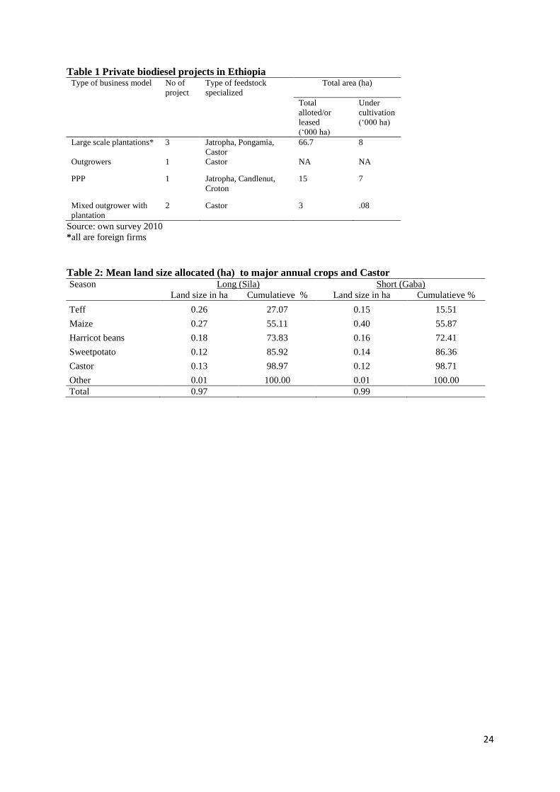
scale plantations and outgrower schemes (table 1).

There are several ways in which rural households can potentially engage in the

biofuel supply chains: (a) through direct employment in large scale plantations, (b)

indirectly through leasing land to biofuel producing companies, (c) through contract

farming schemes with processors (or feedstock exporter) companies, or (d) through small

scale oil extraction schemes. The way biofuel value chains are organized is key to

understand both the impact of biofuels on smallholder famers and the commercial

viability of biofuel production (Altenburg, 2011).

Outgrower schemes are often argued to be more pro-poor than large scale capital

intensive plantations, especially when they result in technology spillovers to other crops

such as observed in Mozambique (Arndt, 2010; Ewing and Msangi, 2009). However,

some recent studies on large scale investments on agriculture question this. For example,

Maertens and Swinnen (2009) and Maertens et al (2011) find that the poorest households

are more likely to benefit from employment on large scale farms than as contract farmers,

based on their studies of horticultural value chains in Senegal. Moreover, achieving

commercial viability in outgrower schemes may be challenging because of large

transaction costs associated with managing production from widely dispersed small farms

and problems of securing a sufficient supply of biofuel feedstock2.

The paper is structured as follows. Section 2 reviews biofuel projects in Ethiopia

and the outgrower scheme. Section 3 describes the sampling design and the data. Section

4 explains the estimation technique. Section 5 gives the results and interpretation of the

results. Section 6 concludes and discusses policy implications.

2 From our interviews with biofuel companies operating in Ethiopia, we learned that some projects were

abandoned because of these reasons.

4

2. Castor production and food security in Ethiopia

The emerging biofuel feedstock production from private firms in Ethiopia thus far is

dominated by two major non-edible crops i.e. castor been and jatropha (see table 1). Castor is

a short season (4-5 months average maturity period) crop that gives oil bearing seeds.

Castor oil contains a toxic element and thus cannot be used as food or animal feed source.

The oil (i.e. biodiesel blended or not) can replace diesel without any engine modification.

Besides, it can be used as lubricant in the automotive field, raw material for cosmetics

industries and in pharmaceuticals. Castor is believed to be indigenous to Ethiopia and grows

both wild and cultivated in the tropical and subtropical countries of the world (Kumar and

Sharma, 2011). It has been promoted in Ethiopia as a commercial crop by foreign companies

during the recent wave of biofuel investments and is said to provide a good base for acquiring

or expanding a profitable position on the world market (Wijnands et al, 2007).

There is an important potential relationship in castor production and food security. The

fact that non-edible sources of feedstock such as castor can potentially be cultivated on

marginal lands makes it less threatening to local food production. However, at the same time,

these marginal areas are often characterized by strong food insecurity.

In Ethiopia policy makers have allocated areas with low agricultural potentials or

degraded areas for the production of biofuel crops. These areas are often recognized as food

insecure areas. For example, one company planted perennial crop trees for biofuel feedstock

on 15,000 ha areas of degraded hills in the Northern region of the country called Kola

Temben, an area known with a large population living under extreme poverty and food

insecurity.

There are also other potential relationships between castor production and food

security, such as the impact of castor production on the productivity of other (food) crops,

5

through rotation or spillovers effects. These effects are likely to depend on the nature of the

production systems (Maertens et al, 2012).

Our study focuses on the contract farming system established by a company in the

Southern region of Ethiopia, more specifically in the Wolayta and Gomo Gofa districts which

are known to be heavily food insecure. Castor production in the Southern region started in

2008 with castor seed distribution to more than 10,000 farm households in Wolayeta and

Gamo Gofa. Farmers traditionally recognize that crop rotation with castor enhances soil

fertility, but no one was interested to cultivate it because of its low value as cash crop. The

company had to undertake extensive promotion activities to introduce the crop as cash crop. It

resulted in widespread adoption (close to 33%) in the third year of the operation.

The company offers a contract to its suppliers. The contract resembles most outgrower

contract schemes where a group of farmers signs a contract to receive all the necessary inputs

such as fertilizer, herbicide, technical assistance. In return they allocate part of their land for

castor production and pay in seeds during harvest. The price of castor seeds is set in advance.

The firm’s extension workers at village level are responsible for training farmers, facilitating

group formation, input distribution and the follow up of cultivation and output collection. The

promoters of the crop are mainly extension agents hired by the company (83%), but

government extension workers have also been involved in disseminating the information.

Land is an important criterion when recruiting farmers; also to make sure that farmers

have enough land to grow the crop and keep adequate land for other crops. Farmers have

been advised both by the government extension workers and the company supervisors not to

allocate more than a quarter of their land to castor. This is also confirmed by our data. The

average allocation of land to castor is 15% of total land covered by annual crops. The

maximum land that farmers allocate does not exceed 25% of the total land holding (table 2).

6

During the initial phase of the project in 2008, a land size of 1ha was a requirement to

allow farmers to engage in a castor contract. But meeting break-even quantity for export was

extremely challenging for the company despite its wide coverage of areas. In the following

years (2009 and 2010) the land size for eligibility was reduced to 0.75ha.

3. Data

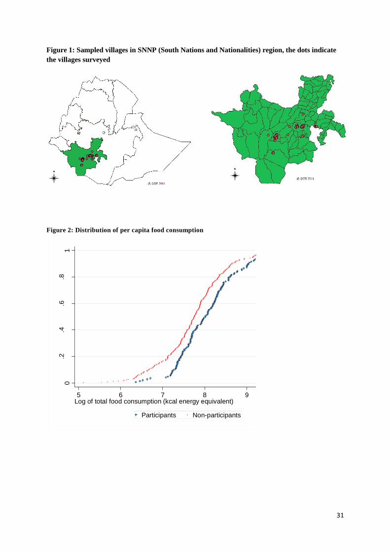
Four districts (woredas) were chosen as representatives of the Wolayeta and Gamo

Gofa administrative zones in the SNNPR region (figure 1). Following a stratified two

stage sampling technique, 24 kebeles (equivalent to villages or a few clusters of villages)

were randomly drawn from those selected districts. The number of sample villages is

proportional to the size of the total number of villages in each district.

All kebeles in each zone that were eligible to grow castor have received castor

seeds with varying degrees of intensity. Castor growing areas of all villages within the

altitude range of 1040 to 2010 meters above sea level were included in our sampling

frame. Our sampling frame has not covered the villages (commonly known as highlands)

that are not agroecologically suitable to grow castor. Thus, the study best represents

smallholder farmers in castor growing areas of the region. We used three sampling

frames: (a) a list of all kebeles and demographic information was obtained from zone

statistics office; (b) a list obtained from the company containing information about

households who received castor seed and their participation history; (c) a 2010 list of all

households who reside in each kebele was collected from each kebele.

18 to 22 households were interviewed in each village and households were

stratified as participants and non-participants in the project. Systematic sampling was

applied to select households from a list, using a random start and with selection intervals

equal to the total number of residents divided by the number of samples to be selected

7

from the entire list. For the actual analysis of this paper, participants (adopters) are

defined as those who participated through receiving castor seeds and inputs in the 2009 -

2010 agricultural year; and non-participants (non-adopters) as those who did not

participate in the project regardless of their past participation history. Participants of 2010

count for 30% of our sample. Since participant samples are close to the actual proportion

in the population (33%), we only applied weights to correct for differences in the sample

proportions.

We conducted the survey in February and March 2011, soon after the main harvest

season. A detailed questionnaire was prepared with questions on crop production,

revenue, input use, income by type, and food security. Except for general household

characteristics, we disaggregated our data enquiry over the two main crop seasons. In

most cases, we interviewed the household head but whenever it was possible we asked

both the head’s and the spouse’s opinion. There were no refusals of interview.

4. Descriptive Statistics

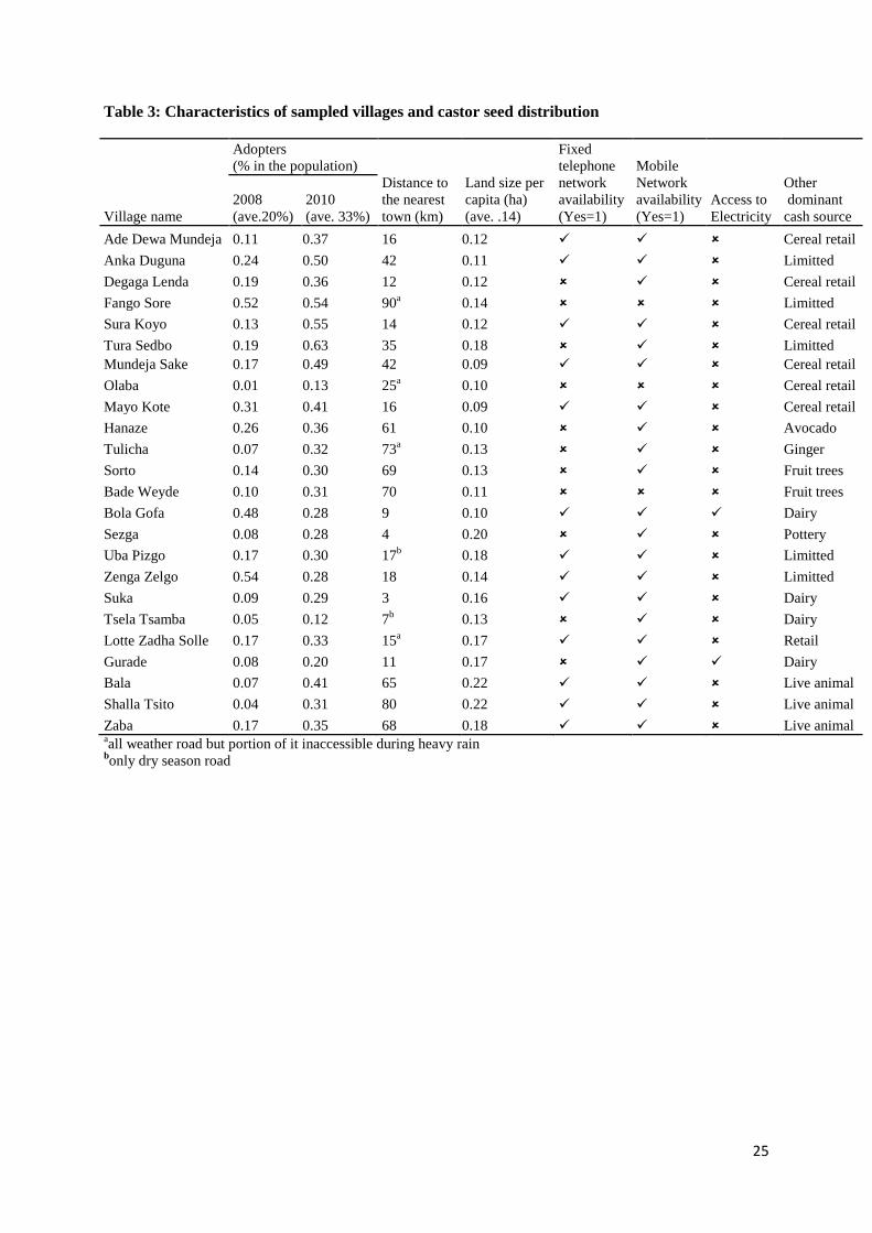
The dataset contains 476 households. About 30% of them are “adopters” , i.e.

households which allocated land to grow castor and received the necessary inputs in the

2010 cropping season. The incidence of adoption over the sample villages is reported in

table 3. The 24 villages in our sample vary in terms of proximity to towns, infrastructure

and other economic activities besides farming. In some villages (such as Fango Sore) that

are far-off from towns and constrained by a limited availability of markets for alternative

commodities, the adoption intensity is above the average rate (54%). Participants and non-

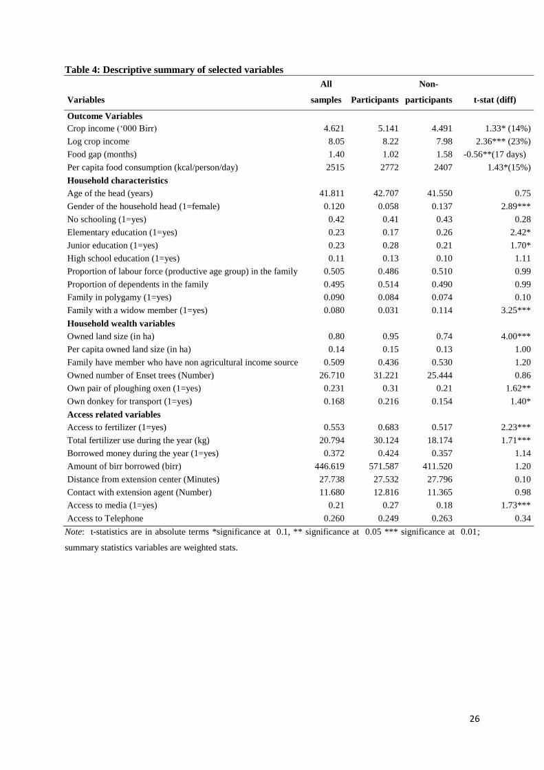
participants differ in certain household characteristics. Female headed households and

widow-headed households are less likely to participate. The proportion of working age

group as well as the number of dependents does not differ between the two groups. There

8

is no strong correlation between education and adoption. Overall, schooling is low: 42%

of the total sample never attended school. Adopter households have a lower proportion of

households with primary education but a higher proportion of households in junior level

education. There is no difference in terms of high school education.

Land holding is a key eligibility criteria for participation, and is significantly

higher for participants. The eligibility criteria has not been enforced strictly. There are

non-participant households who qualify for participation (about 50%) but did not

participate. There are also households that participated but did not formally satisfy the

eligibility criteria

Participants use much more fertilizer (almost double) than non-participants. This

reflects the fact that participants have better fertilizer access through the biofuel contract

scheme.

Participants and non-participants do not differ significantly in terms of proximity to

extension centers, or contact with government extension agents. On average 27% of

participants gets information about markets, prices and agricultural practices primarily

through formal media sources such as radio. Only 18% of non-participants make use of

the formal media sources.

5. Food security indicators

To assess food security, we use two types of measures. The first is the number of

“food gap” months. “Food gap” is defined as the number of months that the household

runs out of its own stock of food (mainly grains and other own livestock food sources) and

lacks money to purchase food’. The study area is known for its severe seasonal fluctuation

in food security. Smoothing intra-year food security at the household level is a prime

concern.

9

Cultivating castor in these areas can be beneficial for food security in many ways.

First, farmers typically have to sell food crops at harvest time when prices of food crops

decline. By generating cash income during the harvest season from castor contracts, they

no longer have to sell food crops and can store them. . Moreover, stocking food would

protect them from having to pay higher prices during the lean seasons. Second, castor

beans planted can be collected twice a year. They preserve well on the field without easily

spoiling like many food crops that need to be harvested immediately. This allows

piecemeal collection of beans and sales to village level collection centers whenever

farmers are in need of cash. For rural farmers liquidity constraints are vital to food security.

For them flexible access to a cash source by being able to harvest and sell whenever

necessary, protects them from taking suboptimal strategies on investments and crop use.

Third, spillover effects on food crops by better access to fertilizer and improved land quality

by rotating castor beans with other crops is another potential channel through which

participant households food security may improve with the scheme.

The length of food gap is on average 1.02 months for adopter households, and 1.58

months for non-participants. This means that non-participant households had more than

50% longer food gaps (0.56 months or 17 days) than participants (table 5). Non-

participants have a significantly larger proportion of households (21%) that experience

more than three months of food gap during the year. Less than 10% of participants

experience such long food gap periods.

As a second indicator of food security, we used per capita food consumption. We

adopt FAO/WFP (2009) guidelines to convert food consumption (both self-produced and

purchased) into energy kilo calorie (kcal) equivalent levels.

10

Table 4 shows that the average food consumption is 2515 kcal per capita per day in

the survey, lower than the national average.3

Table 6 presents the percentage of

households in the categories of different food consumption levels. The data indicate that

food security is high across the survey area, but significantly higher among non-

participants than among participants. 63% of non-participants are food insecure (defined

as having less than 2100 kcal per capita per day) and 42% are chronically food insecure

(defined as having less than 1500 kcal per capita per day). While still high, the numbers

are lower for participants: 51% are food insecure and 36% are chronically food insecure.

6. Econometric Approach

While these descriptive statistics provide useful information on the extent of food

security and the characteristics of participants and non-participants, one cannot draw

conclusions on the casual effect of the outgrower schemes on food security. Adoption of

the new crop is potentially endogenous. One can try to address such endogeneity by

explicitly modeling the simultaneity nature of the equations (Heckman, 1977). However, a

pooled data estimation of both participants and non-participants assumes that the list of

explanatory variables have the same impact on both groups of farmers and implies that

participation has an average effect on the whole sample which may not be necessarily true

due to selection problems (Heckman, 1979)4 .

To account for the differential impact of covariates on the food security of the

different groups, a separate function can be specified and estimated simultaneously

through an endogenous switching regression (ESR) model (Maddala and Nelson, 1983).

Our approach follows recent empirical applications of the model in studying the impact of

3 Berhane et al, 2011 reported 2742 kcal average food consumption in Ethiopia using a more nationally

representative data from Ethiopian CSA (Central Statistics Authority) 4 Refer Wooldridge (2010) for recent reviews of econometric models for program evaluation; and see

Cameron and Trivedi (2010) for their micro empirical applications.

11

choice decisions allowing for endogeneity, sample selection and interaction between

adoption and other covariates that affect the outcome equation (e.g. Alene and Manyong

(2006); Asfaw et al. (2012); Di Falco et al. (2011); Rao and Qaim (2011)). The model

allows to construct the counterfactual expected outcome of the treatment effect under

different regimes (i.e. adopt or not adopt).

Our model follows the specification given by Madalla (1983) and Lee and Trost

(1982). The estimation is implemented using the full information maximum likelihood

(FIML) technique to generate efficient and consistent estimators (Lokshin and Sajaia,

2004). Let denote a dichotomous variable that equals 1 for households observed in

regime 1 (participation in the castor program) and 0 for households in regime 2 (non-

participation).

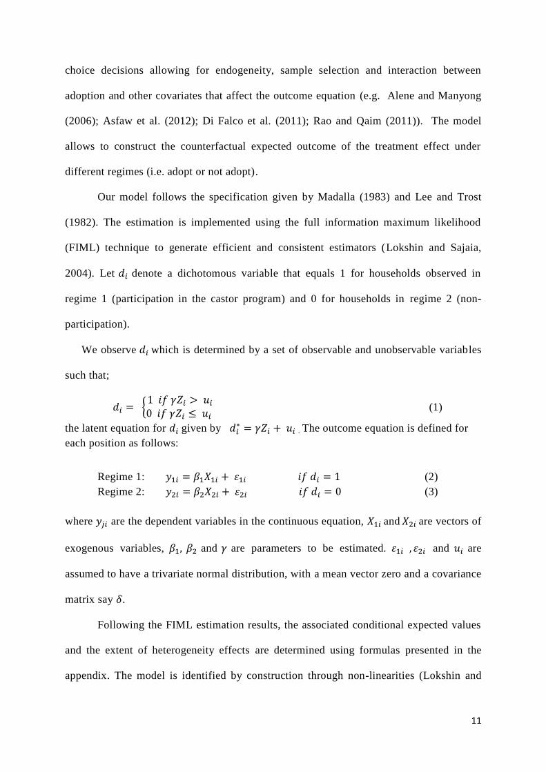
We observe which is determined by a set of observable and unobservable variables

such that;

{

(1)

the latent equation for given by . The outcome equation is defined for

each position as follows:

Regime 1: (2)

Regime 2: (3)

where are the dependent variables in the continuous equation, and are vectors of

exogenous variables, and are parameters to be estimated. and are

assumed to have a trivariate normal distribution, with a mean vector zero and a covariance

matrix say .

Following the FIML estimation results, the associated conditional expected values

and the extent of heterogeneity effects are determined using formulas presented in the

appendix. The model is identified by construction through non-linearities (Lokshin and

12

Sajaia, 2004). However, it is strongly suggested to estimate it with an exclusion restriction

(i.e. that in equation (1) contains at least one variable not in to improve

identification. The variable excluded from needs to be strongly correlated with the

regime choice (equation 1) but not with the outcome variable (Maddala, 1999; Verbeek,

2012; Wooldridge, 2010).

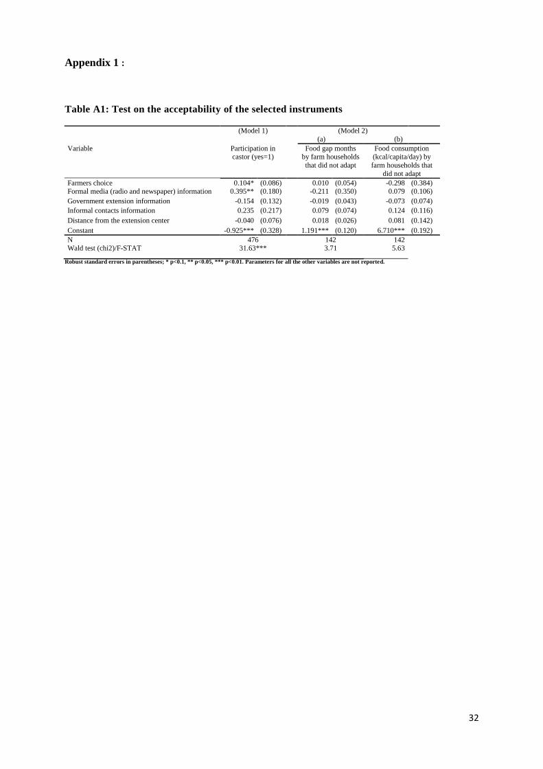
We tried to follow the approach of Di Falco et al (2011) and Asfaw et al (2012) by

using variables related to information sources (e.g. government extension, informal

contacts, information from radio and newspapers). However, of these variables only the

variable capturing information from radio, TV and newspapers satisfied the tests, as the

other were not related to the adaption choice (see table A.1). We therefore constructed

another variable, “farmer eligibility”, following the approach described in Khandker

(2009 p.203). Farmer eligibility is based on a combination of two variables, i.e. (1) the

intensity of past program uptake at the village level, and (2) the eligibility criteria of

participation used by the company to contract farmers i.e. farmers having a land size of

0.75 ha or more. The first variable village-level intensity of program uptake is measured

as the share of the total number of households who received castor seed in the first phase

of the program in the village population.5 The value of the “farmer eligibility” variable is

1 for households who have more than 0.75 hectare of land and who reside in a village

where the intensity of past adoption rate is above the sample mean; and 0 otherwise.6

Table A.1 shows that this variable and the radio, TV and newspaper information variable

both satisfy the criteria for valid selection instruments (they are statistically significant

drivers of the decision to participate (Model 1), but not of the food security indicators

(Model 2a and 2b)). Both are used in the estimations.

5 This ratio is displayed in the second column of table 1.

6 Taking sample median instead of sample mean does not change the result

13

7. Results

7.1 Determinants of the adoption decision

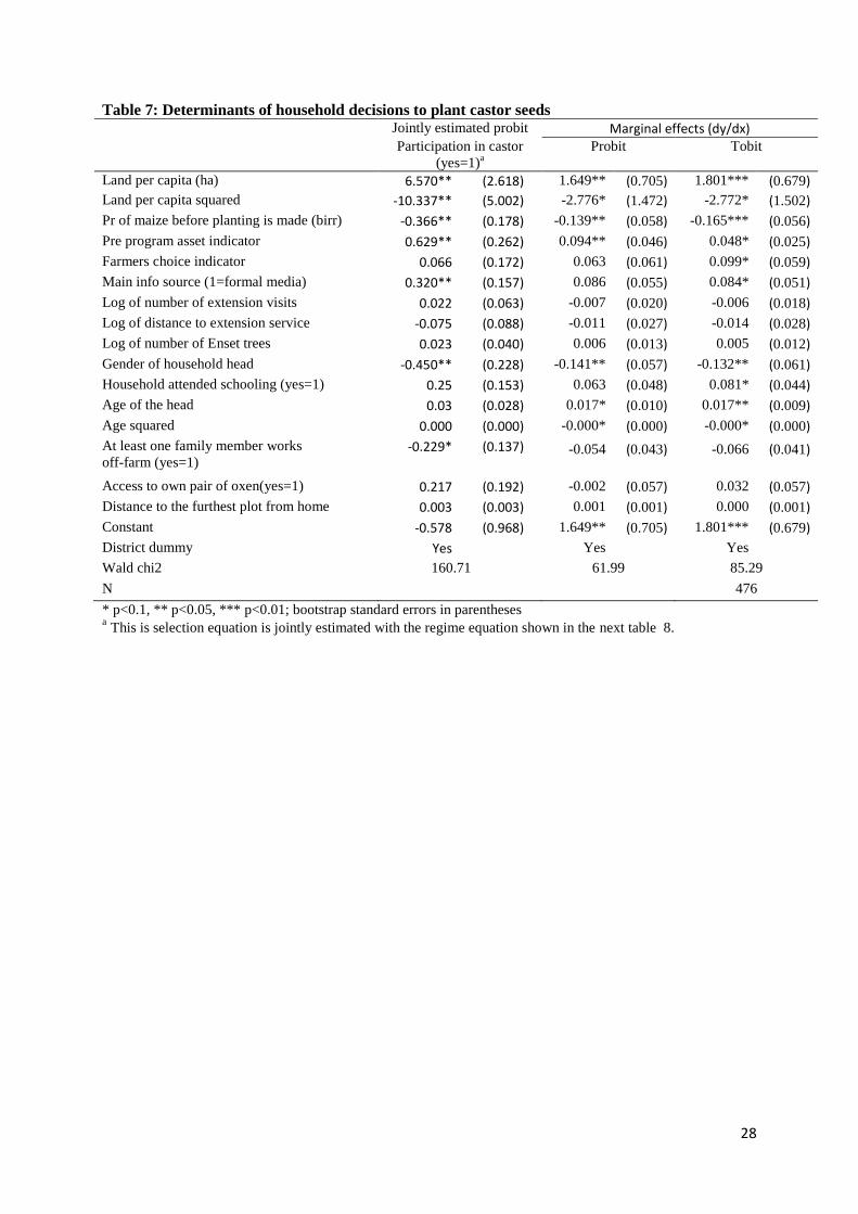
We first run a Probit regression jointly with the food consumption equation to

analyze what factors determine incidence of participation. We controlled for a range of

variables including household characteristics, land size, livestock assets, the price of

maize (at the beginning of the year before planting decisions are made), access to

information and district dummies. For consistency checks (and for calculating marginal

effects), we also estimated an independent Probit and Tobit model. In the Tobit

estimation, the total area each farmer allocates to castor is used as dependent variable.

The estimated coefficients have the expected signs and magnitude. The model fits well

predicting 70% of the observations correctly.

Land size significantly affects adoption, but at a decreasing rate as the squared

term is negative and significant. The combined effect (direct and squared) is positive for

the domain up to 0.31 hectares per capita, which is equivalent of 1.9 hectares per

household for the average household. This is more than twice the eligibility criteria (0.75

hectares per household) and includes almost all the households since 93% of households

are in this domain.

The results further show that a higher price of maize significantly reduces the

allocation of land to castor.7 One birr increase in the price of maize is associated with 0.17

points decline in allocation of land.

The adoption of castor is also correlated with a farmer’s access to formal sources

of information such as radio, TV, and newspapers. Participants tend to depend more on

formal sources of information for their information on agricultural prices and practices

7 Our price data is the average annual market prices in each village in the preceding crop year. In villages where

complete data was absent for some months, we have taken the nearby closest villages price as a proxy.

14

than non-participants who are more reliant on friends, local markets and informal

networks as their primary sources of information.

Like most findings in the literature, the gender of the household head is negatively

and significantly associated with adoption, meaning that women-headed households tend

to adopt less.

Exposure to government extension services does not seem to be an important factor

for adoption. Distance to the extension centers which are often located at the center of

each village is also not significant. The dissemination of the crop was widespread, even in

remote villages. Distance does not appear to be a barrier to adoption.

7.2 Determinants of food security

We estimate the endogenous switching regression using the FIML method. This

model can control for unobservable selection bias under a structural assumption (i.e. the

error terms exhibit independent trivariate distribution). The food equation specifies the

food security outcome variable on the left hand side and endogenous dummy variable for

participation. Control variables include income by type, household characteristics, asset

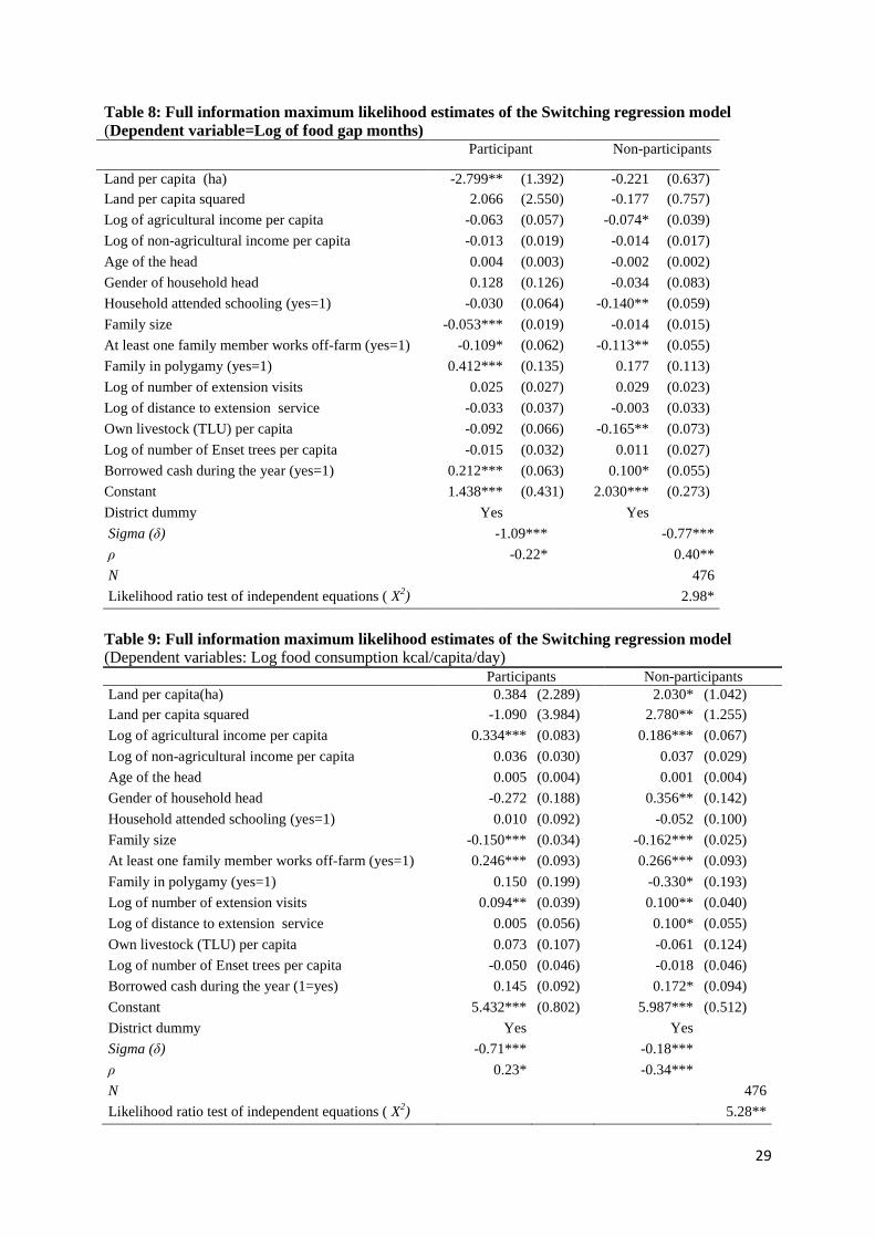
indicators and district dummies. The FIML estimation results for the food gap and food

consumption as dependent variables are reported in tables 8 and 9.

The last rows of table 8 and table 9 show the Log likelihood Ratio (LR) test of the

independence of equations. At a 90% confidence level, it confirms that it was appropriate

to assume that the effects of covariates in the two groups are significantly different. The

opposite signs of the correlation coefficient (ρ) of the two groups imply sorting behavior

of farm households into which they would be better off i.e. participants have higher

returns under adoption while non-participants are better off not participating. The

correlation coefficient of the non-participant outcome equation under the participation

15

equation is positive and significant, suggesting that individuals who choose not to

participate in the castor program would have had higher food gaps than a random

individual from a sample would have, had they participated in the program.

Finally, the suggestions in tables 8 and 9 show that for both participants and non-

participants, off-farm job participation of a family member is significantly linked with

lower food gaps on equal magnitudes. Literacy of the household head is associated with

lower food gaps in both groups, but it is only significant for non-participant households.

Borrowing of more cash during the year, is correlated with higher level of food gaps in

both groups. Households that are food insecure may tend to borrow more during the year.

Estimates of the remaining coefficients, strongly suggests the presence of heterogeneous

effects between the two groups. For example, family size is significantly associated with

lower level of food gaps for participants but not for non-participants. Livestock holding

reduce food gaps significantly for non-participants not for participants.

The implication of some of the determinant variables differ between the food gap

equation and the food consumption equation. Agricultural income determines the level of

food consumption strongly and significantly. However, it contributes relatively less on the

food gap compared to off-farm income. This is an indication that factors which reduce the

food gap may not always be the same as factors that determine total annual food

consumption levels.

7.3 Impact of participation

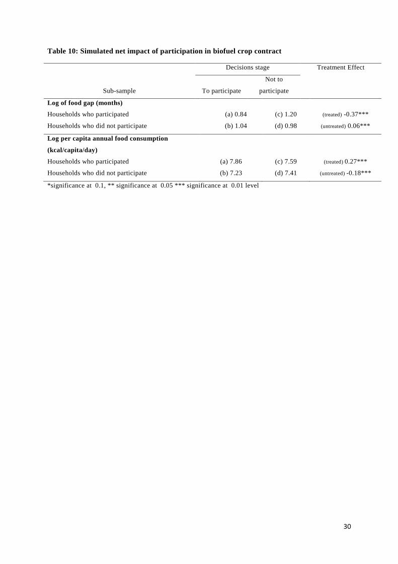
A summary table of impact simulations of participation in Castor outgrower

schemes on food consumption and food gaps are presented in table 10. The values across

the diagonals (in cell (a) and (d)) represent the expected mean values of participants and

non-participants in the sample. The values in cell (b) and (c) are the counterfactual

16

expected values. A positive mean difference of (c) from (a) indicates that participant

farmers gain under participation. A negative mean of (d) from (b) on the contrast, implies

that non-participant farmers perform better under non-participation.

The results show that participation in castor programs has very substantial effects

on food security for the participating households. Participating in castor outgrower

schemes caused an increase in food consumption by more than a quarter (27%) for

participant households. It reduced the number of length of the households’ food gap

period on average by almost a quarter (23%, i.e. 0.37 months compared to the average

foodgap of 1.58 months) for participant households. Hence, participation in the castor

contract provided substantially more food security for adopter households.

In addition, our results also confirm the presence of heterogeneity and sorting

based on comparative advantages. The results show that for non-participants food

consumption would decline and the number of food gap days would increase had they

decided to grow biofuel crop. These households presumably have better alternatives than

the castor program and they fare better, at least in terms of food security, by not

participating. These findings are in line with other studies’ results (e.g. Suri, 2011;

Zeitlin, 2010) that farmers with low expected net returns do not adopt a technology and

the ones who have higher expected returns do apply them.

8. Conclusions

This paper presents micro- evidence on the impact of the cultivation of a biofuel

crop (castor) on food security by presenting survey data and analyzing the effects on poor

households in rural Ethiopia. The study is based on data collected in early 2011 from 478

randomly selected households. We use endogenous switching regression with exclusion

restriction to control for endogenous selection issues in consumption and adoption

17

decisions. Our choice of the instrument is based on the eligibility criteria used by the

contracting company and the pre evaluation period intensity of the program intervention at

the village level.

We find that participating in castor production increased households’ food security

significantly. The effects are substantial and affect both total food consumption and the

periods of food shortages (the food gap). Our findings indicate improvements in both

indicators (increased food consumption and reduced food gap periods) by approximately a

quarter (25%).

Castor production reduces liquidity constraints as they can be harvested at periods of

food shortages and can contribute to mitigate seasonal gaps in food availability. In

addition, participation in the castor programs improves access to fertilizer for these

households, which improves overall crop productivity. This indicates that, in contrast to

many of the arguments being raised, that there is complementarity (instead of

competition) between “fuel” and “food” at the micro-level in castor production in

Ethiopia.

Our analysis also suggests that, not surprisingly, the impact is heterogeneous

across households. We find rational sorting based on comparative advantage from the

technology/crop where participants gain significantly from adopting which they may not

otherwise. Households who do not adapt, appear to do this because they would not

benefit. This is in line with findings of other studies.

There are also important findings on adoption of new crops/technologies. We find

that land and non-land assets are key determinants of castor adoption, while physical

accessibility such as distance from village centers appears not significant for adoption.

These findings are interesting from the perspective of improving the dissemination of new

technologies in poor rural areas. The castor study suggests that this type of privately

18

promoted technologies appear to be quite efficient in overcoming distance barriers –

unlike some other (government-promoted) technologies. This may be an important insight

about the efficiency and the potential role of supply chains in technology dissemination in

the future.

19

References

Ajanovic, A. (2011). Biofuels versus food production: Does biofuels production increase food

prices? Energy, 36(4), 2070–2076.

Alene, A. D., & Manyong, V. M. (2006). The effects of education on agricultural productivity

under traditional and improved technology in northern Nigeria: an endogenous

switching regression analysis. Empirical Economics, 32(1), 141–159.

Altenburg, T. (2011). Interest groups, power relations, and the configuration of value chains:

The case of biodiesel in India. Food Policy, 36(6), 742–748.

Arndt, C., Benfica, R., Tarp, F., & Thurlow, J. (2009). Biofuels, poverty, and growth: a

computable general equilibrium analysis of Mozambique. Environment and

Development Economics, 15(01), 81.

Arndt, C., Msangi, S., & Thurlow, J. (2011). Are biofuels good for African development? An

analytical framework with evidence from Mozambique and Tanzania. Biofuels, 2(2),

221–234.

Asfaw, S., Shiferaw, B., Simtowe, F., & Lipper, L. (2012). Poverty Reduction Effects of

Agricultural Technology Adoption: A Micro-evidence from Rural Tanzania. Journal

of Development Studies. DOI:10.1080/00220388.2012.671475

Berhane, G., Z. Paulos, and K. Tafere. (2011). Foodgrain Consumption and Calorie Intake

Patterns in Ethiopia. ESSP II Working Paper 23. Addis Ababa, Ethiopia: International

Food Policy Research Institute / Ethiopia Strategy Support Program II.

Bindraban, P. S., Bulte, E. H., & Conijn, S. G. (2009). Can large-scale biofuels production be

sustainable by 2020? Agricultural Systems, 101(3), 197–199.

Cameron, A. C., & Trivedi, P. K. (2010). Microeconometrics using Stata. College Station,

Tex.: Stata Press.

Ciaian, P., & Kancs, d’Artis. (2011). Food, energy and environment: Is bioenergy the missing

20

link? Food Policy, 36(5), 571–580.

Cotula, L., Dyer, N., & Vermeulen, S. (2008). Fuelling exclusion? the biofuels boom and

poor people’s access to land. London: IIED.

Cushion, E., Whiteman, A., & Dieterle, G. (2010). Bioenergy development: issues and

impacts for poverty and natural resource management. Washington, D.C.: World

Bank.

Deininger, K. W., Byerlee, D., & Bank, W. (2011). Rising global interest in farmland: can it

yield sustainable and equitable benefits? Washington, D.C.: World Bank.

Dercon, S., Hoddinott, J., & Woldehanna, T. (2011). Growth and chronic poverty: Evidence

from rural communities in Ethiopia. CSAE Working Paper.

Devereux, S., & Guenther, B. (2009). Agriculture and social protection. FAC (Future

Agriculture Consortium) Working Paper.

Di Falco, S., Veronesi, M., & Yesuf, M. (2011). Does Adaptation to Climate Change Provide

Food Security? A Micro-Perspective from Ethiopia. American Journal of Agricultural

Economics, 93(3), 829–846.

Ewing, M., & Msangi, S. (2009). Biofuels production in developing countries: assessing

tradeoffs in welfare and food security. Environmental Science & Policy, 12(4), 520–

528.

FAO (Food and Agriculture Organization). (2008). Biofules: prospects, risks and

opportunities. The state of food and agriculture. Rome: FAO.

FAO (Food and Agriculture Organization), & WFP (World Food Program). (2009). Joiint

Guidelines January 2009 for Crop and Food Security Assessment Missions. Rome:

FAO and WFP.

Fargione, J., Hill, J., Tilman, D., Polasky, S., & Hawthorne, P. (2008). Land Clearing and the

Biofuel Carbon Debt. Science, 319(5867), 1235–1238.

21

Heckman, J. (1979). Sample Selection Bias as a Specification Error. Econometrica, 47(1),

153–161.

Hung, J., Yang, J., Msangi, S., Rosegrant, M., Rozelle, S., & Weersink, A. (Forthcoming).

Biofuels, Food Secuirty and the Poor: Global Impact Pathways of Biofuels on

Agricultural Markets. Food Policy.

IIED (International Institute for Environment and Development). (2009). Biofuel in Africa:

growing small-scale opportunities (Briefing business models for sustainable

development). London: IIDA.

Khandker, Shahidur R., Gayatri B. Koolwal, and Hussain Samad. (2009). Handbook

on Quantitative Methods of Program Evaluation. Washington, DC: World Bank.

Kumar, A., & Sharma, S. (2011). Potential non-edible oil resources as biodiesel feedstock: An

Indian perspective. Renewable and Sustainable Energy Reviews, 15(4), 1791–1800.

Lee, L.-F., & Trost, R. P. (1978). Estimation of some limited dependent variable models with

application to housing demand. Journal of Econometrics, 8(3), 357–382.

Lokshin, M., & Sajaia, Z. (2004). Maximum Likelihood Estimation of Endogenous Switching

Regression Models. Stata Journal, 4(3), 282–289.

Maddala, G. S. (1999). Limited-dependent and qualitative variables in econometrics.

Cambridge [u.a.]: Cambridge Univ. Press.

Maddala, G. S., & Nelson, F. S. (1975). Switching Regression Models with Exogenous and

Endogenous Switching. Proceeding of the American Statistical Association, Business

and Economics Section.

Maertens, M., Minten, B. and J. Swinnen (2012) Modern Food Supply Chains and

Development: Evidence from Horticulture Export Sectors in Sub-Saharan Africa.

Development Policy Review, forthcoming.

Maertens, M., Colen, L., & Swinnen, J. F. M. (2011). Globalisation and poverty in Senegal: a

22

worst case scenario? European Review of Agricultural Economics, 38(1), 31–54.

Maertens, Miet, & Swinnen, J. F. M. (2009). Trade, Standards, and Poverty: Evidence from

Senegal. World Development, 37(1), 161–178.

Mare, R., & Winship, C. (1987). Endogenous Switching Regresstion Models for the causes

and effects of discrete variables. CDE. Working paper, Wisconsin. Retrieved from

Mitchell, D. (2008). A Note on Rising Food Prices. Policy Research Working Paper.

Nussbaumer, P., Bazilian, M., & Modi, V. (2012). Measuring energy poverty: Focusing on

what matters. Renewable and Sustainable Energy Reviews, 16(1), 231–243.

Pimentel, D., Marklein, A., Toth, M. A., Karpoff, M. N., Paul, G. S., McCormack, R.,

Kyriazis, J., et al. (2009). Food Versus Biofuels: Environmental and Economic Costs.

Human Ecology, 37(1), 1–12.

Rao, E. J. O., & Qaim, M. (2011). Supermarkets, Farm Household Income, and Poverty:

Insights from Kenya. World Development, 39(5), 784–796.

Suri, T. (2011). Selection and Comparative Advantage in Technology Adoption.

Econometrica, 79(1), 159–209.

Taheripour, F., Hertel, T. W., Tyner, W. E., Beckman, J. F., & Birur, D. K. (2010). Biofuels

and their by-products: Global economic and environmental implications. Biomass and

Bioenergy, 34(3), 278–289.

Verbeek, M. (2012). A guide to modern econometrics. Hoboken, NJ: Wiley.

Wijnands, J., Biersteker, J., & Hiel, R. (2007). Oilseeds business opportunities in Ethiopia.

Unpublished manscript, The Heague.

Wooldridge, J. M. (2008). Instrumental variables estimation of the average treatment effect in

the correlated random coefficient model. Advances in Econometrics (Vol. 21, pp. 93–

116). Bingley: Emerald (MCB UP ).

Wooldridge, J. M. (2010). Econometric analysis of cross section and panel data. Cambridge,

23

Mass.: MIT Press.

Zeitlin, A., Teal, F., Caria, S., Dzene, R., & Opoku, E. (2010). Heterogeneous returns and the

persistence of agricultural technology adoption. CSAE Discussion paper, Oxford

University.

24

Table 1 Private biodiesel projects in Ethiopia Type of business model No of

project

Type of feedstock

specialized

Total area (ha)

Total

alloted/or

leased

(‘000 ha)

Under

cultivation

(‘000 ha)

Large scale plantations* 3 Jatropha, Pongamia,

Castor

66.7 8

Outgrowers 1 Castor NA NA

PPP 1 Jatropha, Candlenut,

Croton

15 7

Mixed outgrower with

plantation

2 Castor 3 .08

Source: own survey 2010

*all are foreign firms

Table 2: Mean land size allocated (ha) to major annual crops and Castor Season Long (Sila) Short (Gaba)

Land size in ha Cumulatieve % Land size in ha Cumulatieve %

Teff 0.26 27.07 0.15 15.51

Maize 0.27 55.11 0.40 55.87

Harricot beans 0.18 73.83 0.16 72.41

Sweetpotato 0.12 85.92 0.14 86.36

Castor 0.13 98.97 0.12 98.71

Other 0.01 100.00 0.01 100.00

Total 0.97

0.99

25

Table 3: Characteristics of sampled villages and castor seed distribution

Village name

Adopters

(% in the population)

Distance to

the nearest

town (km)

Land size per

capita (ha)

(ave. .14)

Fixed

telephone

network

availability

(Yes=1)

Mobile

Network

availability

(Yes=1)

Access to

Electricity

Other

dominant

cash source

2008

(ave.20%)

2010

(ave. 33%)

Ade Dewa Mundeja 0.11 0.37 16 0.12 Cereal retail

Anka Duguna 0.24 0.50 42 0.11 Limitted

Degaga Lenda 0.19 0.36 12 0.12 Cereal retail

Fango Sore 0.52 0.54 90a 0.14 Limitted

Sura Koyo 0.13 0.55 14 0.12 Cereal retail

Tura Sedbo 0.19 0.63 35 0.18 Limitted

Mundeja Sake 0.17 0.49 42 0.09 Cereal retail

Olaba 0.01 0.13 25a 0.10 Cereal retail

Mayo Kote 0.31 0.41 16 0.09 Cereal retail

Hanaze 0.26 0.36 61 0.10 Avocado

Tulicha 0.07 0.32 73a 0.13 Ginger

Sorto 0.14 0.30 69 0.13 Fruit trees

Bade Weyde 0.10 0.31 70 0.11 Fruit trees

Bola Gofa 0.48 0.28 9 0.10 Dairy

Sezga 0.08 0.28 4 0.20 Pottery

Uba Pizgo 0.17 0.30 17b 0.18 Limitted

Zenga Zelgo 0.54 0.28 18 0.14 Limitted

Suka 0.09 0.29 3 0.16 Dairy

Tsela Tsamba 0.05 0.12 7b 0.13 Dairy

Lotte Zadha Solle 0.17 0.33 15a 0.17 Retail

Gurade 0.08 0.20 11 0.17 Dairy

Bala 0.07 0.41 65 0.22 Live animal

Shalla Tsito 0.04 0.31 80 0.22 Live animal

Zaba 0.17 0.35 68 0.18 Live animal aall weather road but portion of it inaccessible during heavy rain

bonly dry season road

26

Table 4: Descriptive summary of selected variables

Variables

All

samples Participants

Non-

participants t-stat (diff)

Outcome Variables

Crop income (‘000 Birr) 4.621 5.141 4.491 1.33* (14%)

Log crop income 8.05 8.22 7.98 2.36*** (23%)

Food gap (months) 1.40 1.02 1.58 -0.56**(17 days)

Per capita food consumption (kcal/person/day) 2515 2772 2407 1.43*(15%)

Household characteristics

Age of the head (years) 41.811 42.707 41.550 0.75

Gender of the household head (1=female) 0.120 0.058 0.137 2.89***

No schooling (1=yes) 0.42 0.41 0.43 0.28

Elementary education (1=yes) 0.23 0.17 0.26 2.42*

Junior education (1=yes) 0.23 0.28 0.21 1.70*

High school education (1=yes) 0.11 0.13 0.10 1.11

Proportion of labour force (productive age group) in the family 0.505 0.486 0.510 0.99

Proportion of dependents in the family 0.495 0.514 0.490 0.99

Family in polygamy (1=yes) 0.090 0.084 0.074 0.10

Family with a widow member (1=yes) 0.080 0.031 0.114 3.25***

Household wealth variables

Owned land size (in ha) 0.80 0.95 0.74 4.00***

Per capita owned land size (in ha) 0.14 0.15 0.13 1.00

Family have member who have non agricultural income source

(1=yes)

0.509 0.436 0.530 1.20

Owned number of Enset trees (Number) 26.710 31.221 25.444 0.86

Own pair of ploughing oxen (1=yes) 0.231 0.31 0.21 1.62**

Own donkey for transport (1=yes) 0.168 0.216 0.154 1.40*

Access related variables

Access to fertilizer (1=yes) 0.553 0.683 0.517 2.23***

Total fertilizer use during the year (kg) 20.794 30.124 18.174 1.71***

Borrowed money during the year (1=yes) 0.372 0.424 0.357 1.14

Amount of birr borrowed (birr) 446.619 571.587 411.520 1.20

Distance from extension center (Minutes) 27.738 27.532 27.796 0.10

Contact with extension agent (Number) 11.680 12.816 11.365 0.98

Access to media (1=yes) 0.21 0.27 0.18 1.73***

Access to Telephone 0.260 0.249 0.263 0.34

Note: t-statistics are in absolute terms *significance at 0.1, ** significance at 0.05 *** significance at 0.01;

summary statistics variables are weighted stats.

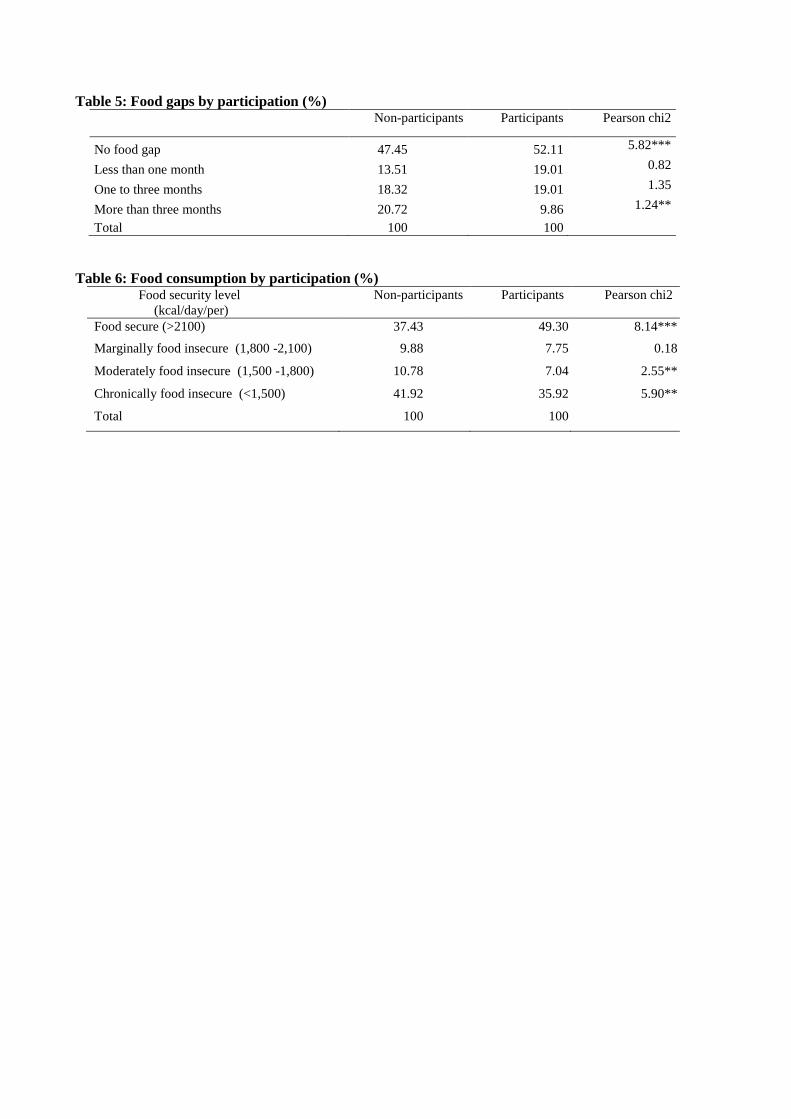
Table 5: Food gaps by participation (%)

Non-participants Participants Pearson chi2

No food gap 47.45 52.11 5.82***

Less than one month 13.51 19.01 0.82

One to three months 18.32 19.01 1.35

More than three months 20.72 9.86 1.24**

Total 100 100

Table 6: Food consumption by participation (%) Food security level

(kcal/day/per)

Non-participants Participants Pearson chi2

Food secure (>2100) 37.43 49.30 8.14***

Marginally food insecure (1,800 -2,100) 9.88 7.75 0.18

Moderately food insecure (1,500 -1,800) 10.78 7.04 2.55**

Chronically food insecure (<1,500) 41.92 35.92 5.90**

Total 100 100

28

Table 7: Determinants of household decisions to plant castor seeds Jointly estimated probit Marginal effects (dy/dx)

Participation in castor

(yes=1)a

Probit Tobit

Land per capita (ha) 6.570** (2.618) 1.649** (0.705) 1.801*** (0.679)

Land per capita squared -10.337** (5.002) -2.776* (1.472) -2.772* (1.502)

Pr of maize before planting is made (birr) -0.366** (0.178) -0.139** (0.058) -0.165*** (0.056)

Pre program asset indicator 0.629** (0.262) 0.094** (0.046) 0.048* (0.025)

Farmers choice indicator 0.066 (0.172) 0.063 (0.061) 0.099* (0.059)

Main info source (1=formal media) 0.320** (0.157) 0.086 (0.055) 0.084* (0.051)

Log of number of extension visits 0.022 (0.063) -0.007 (0.020) -0.006 (0.018)

Log of distance to extension service -0.075 (0.088) -0.011 (0.027) -0.014 (0.028)

Log of number of Enset trees 0.023 (0.040) 0.006 (0.013) 0.005 (0.012)

Gender of household head -0.450** (0.228) -0.141** (0.057) -0.132** (0.061)

Household attended schooling (yes=1) 0.25 (0.153) 0.063 (0.048) 0.081* (0.044)

Age of the head 0.03 (0.028) 0.017* (0.010) 0.017** (0.009)

Age squared 0.000 (0.000) -0.000* (0.000) -0.000* (0.000)

At least one family member works

off-farm (yes=1) -0.229* (0.137) -0.054 (0.043) -0.066 (0.041)

Access to own pair of oxen(yes=1) 0.217 (0.192) -0.002 (0.057) 0.032 (0.057)

Distance to the furthest plot from home 0.003 (0.003) 0.001 (0.001) 0.000 (0.001)

Constant -0.578 (0.968) 1.649** (0.705) 1.801*** (0.679)

District dummy Yes Yes Yes

Wald chi2 160.71 61.99 85.29

N 476

* p<0.1, ** p<0.05, *** p<0.01; bootstrap standard errors in parentheses a This is selection equation is jointly estimated with the regime equation shown in the next table 8.

29

Table 8: Full information maximum likelihood estimates of the Switching regression model

(Dependent variable=Log of food gap months) Participant Non-participants

Land per capita (ha) -2.799** (1.392) -0.221 (0.637)

Land per capita squared 2.066 (2.550) -0.177 (0.757)

Log of agricultural income per capita -0.063 (0.057) -0.074* (0.039)

Log of non-agricultural income per capita -0.013 (0.019) -0.014 (0.017)

Age of the head 0.004 (0.003) -0.002 (0.002)

Gender of household head 0.128 (0.126) -0.034 (0.083)

Household attended schooling (yes=1) -0.030 (0.064) -0.140** (0.059)

Family size -0.053*** (0.019) -0.014 (0.015)

At least one family member works off-farm (yes=1) -0.109* (0.062) -0.113** (0.055)

Family in polygamy (yes=1) 0.412*** (0.135) 0.177 (0.113)

Log of number of extension visits 0.025 (0.027) 0.029 (0.023)

Log of distance to extension service -0.033 (0.037) -0.003 (0.033)

Own livestock (TLU) per capita -0.092 (0.066) -0.165** (0.073)

Log of number of Enset trees per capita -0.015 (0.032) 0.011 (0.027)

Borrowed cash during the year (yes=1) 0.212*** (0.063) 0.100* (0.055)

Constant 1.438*** (0.431) 2.030*** (0.273)

District dummy Yes Yes

Sigma (δ) -1.09*** -0.77***

ρ -0.22* 0.40**

N 476

Likelihood ratio test of independent equations ( X2) 2.98*

Table 9: Full information maximum likelihood estimates of the Switching regression model

(Dependent variables: Log food consumption kcal/capita/day)

Participants Non-participants

Land per capita(ha) 0.384 (2.289) 2.030* (1.042)

Land per capita squared -1.090 (3.984) 2.780** (1.255)

Log of agricultural income per capita 0.334*** (0.083) 0.186*** (0.067)

Log of non-agricultural income per capita 0.036 (0.030) 0.037 (0.029)

Age of the head 0.005 (0.004) 0.001 (0.004)

Gender of household head -0.272 (0.188) 0.356** (0.142)

Household attended schooling (yes=1) 0.010 (0.092) -0.052 (0.100)

Family size -0.150*** (0.034) -0.162*** (0.025)

At least one family member works off-farm (yes=1) 0.246*** (0.093) 0.266*** (0.093)

Family in polygamy (yes=1) 0.150 (0.199) -0.330* (0.193)

Log of number of extension visits 0.094** (0.039) 0.100** (0.040)

Log of distance to extension service 0.005 (0.056) 0.100* (0.055)

Own livestock (TLU) per capita 0.073 (0.107) -0.061 (0.124)

Log of number of Enset trees per capita -0.050 (0.046) -0.018 (0.046)

Borrowed cash during the year (1=yes) 0.145 (0.092) 0.172* (0.094)

Constant 5.432*** (0.802) 5.987*** (0.512)

District dummy Yes Yes

Sigma (δ) -0.71*** -0.18***

ρ 0.23* -0.34***

N 476

Likelihood ratio test of independent equations ( X2) 5.28**

30

Table 10: Simulated net impact of participation in biofuel crop contract

Sub-sample

Decisions stage Treatment Effect

To participate

Not to

participate

Log of food gap (months)

Households who participated (a) 0.84 (c) 1.20 (treated) -0.37***

Households who did not participate (b) 1.04 (d) 0.98 (untreated) 0.06***

Log per capita annual food consumption

(kcal/capita/day)

Households who participated (a) 7.86 (c) 7.59 (treated) 0.27***

Households who did not participate (b) 7.23 (d) 7.41 (untreated) -0.18***

*significance at 0.1, ** significance at 0.05 *** significance at 0.01 level

31

Figure 1: Sampled villages in SNNP (South Nations and Nationalities) region, the dots indicate

the villages surveyed

Figure 2: Distribution of per capita food consumption

0.2

.4.6

.81

Cum

ilative fra

ction

of ho

use

ho

lds

5 6 7 8 9 10Log of total food consumption (kcal energy equivalent)

Participants Non-participants

32

Appendix 1 :

Table A1: Test on the acceptability of the selected instruments

(Model 1) (Model 2)

(a) (b)

Variable Participation in castor (yes=1)

Food gap months by farm households

that did not adapt

Food consumption (kcal/capita/day) by

farm households that

did not adapt

Farmers choice 0.104* (0.086) 0.010 (0.054) -0.298 (0.384) Formal media (radio and newspaper) information 0.395** (0.180) -0.211 (0.350) 0.079 (0.106)

Government extension information -0.154 (0.132) -0.019 (0.043) -0.073 (0.074)

Informal contacts information 0.235 (0.217) 0.079 (0.074) 0.124 (0.116)

Distance from the extension center -0.040 (0.076) 0.018 (0.026) 0.081 (0.142)

Constant -0.925*** (0.328) 1.191*** (0.120) 6.710*** (0.192)

N 476 142 142 Wald test (chi2)/F-STAT 31.63*** 3.71 5.63

Robust standard errors in parentheses; * p<0.1, ** p<0.05, *** p<0.01. Parameters for all the other variables are not reported.

33