University of Alberta

Library Release Form

Name of Author: Yasin Abbasi-Yadkori

Title of Thesis: Forced-Exploration Based Algorithms for Playing in Bandits with LargeAction Sets

Degree: Master of Science

Year this Degree Granted: 2009

Permission is hereby granted to the University of Alberta Library to reproduce single copiesof this thesis and to lend or sell such copies for private, scholarly or scientific researchpurposes only.

The author reserves all other publication and other rights in association with the copyrightin the thesis, and except as herein before provided, neither the thesis nor any substantialportion thereof may be printed or otherwise reproduced in any material form whateverwithout the author’s prior written permission.

Yasin Abbasi-Yadkori4071 - 33A StreetEdmonton, AlbertaCanada, T6T-1R4

Date:

University of Alberta

Forced-Exploration Based Algorithms for Playing in Banditswith Large Action Sets

by

Yasin Abbasi-Yadkori

A thesis submitted to the Faculty of Graduate Studies and Research in partial fulfillmentof the requirements for the degree of Master of Science.

in

Computing Science

Department of Computing Science

Edmonton, AlbertaSpring 2009

University of Alberta

Faculty of Graduate Studies and Research

The undersigned certify that they have read, and recommend to the Faculty of GraduateStudies and Research for acceptance, a thesis entitled Forced-Exploration Based Algo-rithms for Playing in Bandits with Large Action Sets submitted by Yasin Abbasi-Yadkori in partial fulfillment of the requirements for the degree of Master of Science inComputing Science.

Csaba Szepesvari

Dale Schuurmans

Edit Gombay

Date:

Abstract

We study the bandit problem when the payoff function (a) is linear in actions or (b) satisfies

some smoothness conditions. For each structure, we upper bound the regret of the Forced

Exploration algorithm. The main objective of this thesis is to show what we can achieve by

using the Forced Exploration algorithm.

For the linear case, we propose an algorithm, called FEL, and prove that its regret at

time T is upper bounded by d√T + O

(√T

dν2d

), where d is the number of features and νd is

the smallest eigenvalue of the dispersion matrix. Our experiments support our upper bound

and show that FEL outperforms some alternative algorithms when there are correlations

between the payoffs of the actions. When there are no such correlations, the UCT Algorithm

of Kocsis and Szepesvari (2006) outperforms FEL.

For the smooth payoff case, we propose an algorithm with a regret bounded by O(T2+α2+2α ),

where α ∈ N is the differentiability of the payoff function that must be known to the

algorithm. The state of the art result for this problem is due to Auer et al. (2007) who

propose an algorithm with a regret bounded byO(T1+α−αβ1+2α−αβ ) where β is a problem-dependent

parameter. The advantage of our algorithm is that it allows a flexible combination of known

payoff structures with a non-parametric approach.

iii

Acknowledgements

iv

Table of Contents

1 Introduction 11.1 K-armed Bandit Problems . . . . . . . . . . . . . . . . . . . . . . . . . . . . . 11.2 Bandit Problems with Large Action Sets . . . . . . . . . . . . . . . . . . . . . 5

1.2.1 Stochastic Linear Bandit Problems . . . . . . . . . . . . . . . . . . . . 61.2.2 Associative Linear Bandits . . . . . . . . . . . . . . . . . . . . . . . . 81.2.3 Continuum-armed Bandit Problems . . . . . . . . . . . . . . . . . . . 9

2 Playing in Parametric Bandit Problems 122.1 Analysis of Least Squares Solution . . . . . . . . . . . . . . . . . . . . . . . . 13

2.1.1 Bounding E[∥∥∥C−1

t Ht

∥∥∥2

2

]. . . . . . . . . . . . . . . . . . . . . . . . . 16

2.1.2 Bounding E[λmax(D2

t )]

. . . . . . . . . . . . . . . . . . . . . . . . . . 222.1.3 Putting all together . . . . . . . . . . . . . . . . . . . . . . . . . . . . 24

2.2 FEL Analysis . . . . . . . . . . . . . . . . . . . . . . . . . . . . . . . . . . . . 252.3 Results For Various Action Sets . . . . . . . . . . . . . . . . . . . . . . . . . . 27

2.3.1 Generalized Linear Payoff . . . . . . . . . . . . . . . . . . . . . . . . . 30

3 Non-parametric Bandits 313.1 FEC Analysis . . . . . . . . . . . . . . . . . . . . . . . . . . . . . . . . . . . . 31

4 Experiments 414.1 Scaling with d and T . . . . . . . . . . . . . . . . . . . . . . . . . . . . . . . . 414.2 The Ad Allocation Problem . . . . . . . . . . . . . . . . . . . . . . . . . . . . 434.3 FEL vs. UCT . . . . . . . . . . . . . . . . . . . . . . . . . . . . . . . . . . . . 45

5 Conclusions 48

A Background in Calculus 51

B Exponential Tail Inequalities 53

0

Chapter 1

Introduction

Sequential decision making problems such as web advertising (Pandey et al., 2007), design of

clinical trials (Thompson, 1933), sequential design of experiments (Lai and Robbins, 1985),

and online pricing (Kleinberg, 2005) are often formulated as bandit problems. Pick a set of

actions A. In a bandit problem at time t a learner takes some action (also called an arm)

At ∈ A and receives a reward Yt such that

Yt = h(At) + Zt,

where h is an unknown function and Zt is a zero-mean noise. The objective is to minimize

the regret,

R(T ) = T maxa∈A

h(a)−T∑t=1

h(At), (1.1)

where T is the time horizon.

The bandit problem has been studied for various action spaces. The most widely studied

version of the bandit problem is the K-armed bandit problem where the action space is finite,

A = 1, 2, . . . ,K (Robbins, 1952). Here we are interested in problems where the action

space is large, or infinite. Before describing our approach we provide a brief overview of

the relevant literature. In particular, a literature review for the K-armed bandit problem is

presented in Section 1.1, while Section 1.2 provides a literature review for the case when A

is very large or continuous.

1.1 K-armed Bandit Problems

In this chapter, we describe the K-armed bandit problem and a few algorithms proposed

to solve it. We use i = 1, . . . ,K = A to denote the actions in the action space. Further,

we let hi denote the mean payoff of action i, Yi,t be its random payoff at time t, and

h∗ = maxi hi be the mean payoff of the optimal action. Let Yi,Ti(t) be the average of the

first Ti(t) payoffs of action i, where Ti(t) is the number of times we have played action i up

to time t.

1

Let f0 := 0, Si(0) := 0 and Ti(0) := 0 for i = 1, . . . ,Kfor t := 1, 2, . . . do

if ft−1 < f∗t thenExploration:it ∼ P Draw a random action from A according to distribution Pft := ft−1 + 1

elseExploitation:it := argmaxi Yi,Ti(t)

end ifPlay it and receive payoff Yit,tfor i := 1, . . . ,K doTi(t) := Ti(t− 1) + Ii=itSi(t) := Si(t− 1) + Ii=itYit,tYi,Ti(t) := Si(t)/Ti(t)

end forend for

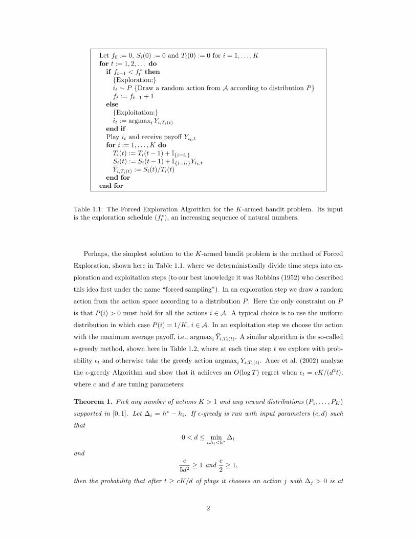
Table 1.1: The Forced Exploration Algorithm for the K-armed bandit problem. Its inputis the exploration schedule (f∗t ), an increasing sequence of natural numbers.

Perhaps, the simplest solution to the K-armed bandit problem is the method of Forced

Exploration, shown here in Table 1.1, where we deterministically divide time steps into ex-

ploration and exploitation steps (to our best knowledge it was Robbins (1952) who described

this idea first under the name “forced sampling”). In an exploration step we draw a random

action from the action space according to a distribution P . Here the only constraint on P

is that P (i) > 0 must hold for all the actions i ∈ A. A typical choice is to use the uniform

distribution in which case P (i) = 1/K, i ∈ A. In an exploitation step we choose the action

with the maximum average payoff, i.e., argmaxi Yi,Ti(t). A similar algorithm is the so-called

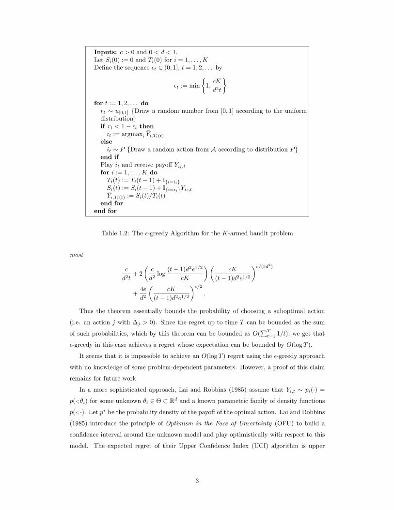
ε-greedy method, shown here in Table 1.2, where at each time step t we explore with prob-

ability εt and otherwise take the greedy action argmaxi Yi,Ti(t). Auer et al. (2002) analyze

the ε-greedy Algorithm and show that it achieves an O(log T ) regret when εt = cK/(d2t),

where c and d are tuning parameters:

Theorem 1. Pick any number of actions K > 1 and any reward distributions (P1, . . . , PK)

supported in [0, 1]. Let ∆i = h∗ − hi. If ε-greedy is run with input parameters (c, d) such

that

0 < d ≤ mini:hi<h∗

∆i

andc

5d2≥ 1 and

c

2≥ 1,

then the probability that after t ≥ cK/d of plays it chooses an action j with ∆j > 0 is at

2

Inputs: c > 0 and 0 < d < 1.Let Si(0) := 0 and Ti(0) for i = 1, . . . ,KDefine the sequence εt ∈ (0, 1], t = 1, 2, . . . by

εt := min

1,cK

d2t

for t := 1, 2, . . . dort ∼ u[0,1] Draw a random number from [0, 1] according to the uniformdistributionif rt < 1− εt thenit := argmaxi Yi,Ti(t)

elseit ∼ P Draw a random action from A according to distribution P

end ifPlay it and receive payoff Yit,tfor i := 1, . . . ,K doTi(t) := Ti(t− 1) + Ii=itSi(t) := Si(t− 1) + Ii=itYit,tYi,Ti(t) := Si(t)/Ti(t)

end forend for

Table 1.2: The ε-greedy Algorithm for the K-armed bandit problem

most

c

d2t+ 2

(c

d2log

(t− 1)d2e1/2

cK

)(cK

(t− 1)d2e1/2

)c/(5d2)

+4ed2

(cK

(t− 1)d2e1/2

)c/2.

Thus the theorem essentially bounds the probability of choosing a suboptimal action

(i.e. an action j with ∆j > 0). Since the regret up to time T can be bounded as the sum

of such probabilities, which by this theorem can be bounded as O(∑Tt=1 1/t), we get that

ε-greedy in this case achieves a regret whose expectation can be bounded by O(log T ).

It seems that it is impossible to achieve an O(log T ) regret using the ε-greedy approach

with no knowledge of some problem-dependent parameters. However, a proof of this claim

remains for future work.

In a more sophisticated approach, Lai and Robbins (1985) assume that Yi,t ∼ pi(·) =

p(·; θi) for some unknown θi ∈ Θ ⊂ Rd and a known parametric family of density functions

p(·; ·). Let p∗ be the probability density of the payoff of the optimal action. Lai and Robbins

(1985) introduce the principle of Optimism in the Face of Uncertainty (OFU) to build a

confidence interval around the unknown model and play optimistically with respect to this

model. The expected regret of their Upper Confidence Index (UCI) algorithm is upper

3

Let Si(0) := 0, Ti(0) := 0 and Yi,0 := 0 for i = 1, . . . ,Kfor t := 1, 2, . . . do

it := argmaxi(Yi,Ti(t−1) +

√2 log(t−1)Ti(t−1)

)Play it and receive payoff Yit,tfor i := 1, . . . ,K doTi(t) := Ti(t− 1) + Ii=itSi(t) := Si(t− 1) + Ii=itYit,tYi,Ti(t) := Si(t)/Ti(t)

end forend for

Table 1.3: The UCB1 Algorithm for the K-armed bandit problem. By convention we letc/0 = +∞. This makes the algorith select each action once at the beginning.

bounded by (1/D(pj ||p∗) + o(1)) log(T ), where

D(pj ||p∗) =∫pj(x) log

pj(x)p∗(x)

dx

is the Kullback-Leibler divergence between pj and p∗. They also prove a lower bound for this

problem that matches their upper bound up to sublogarithmic (o(log T )) terms, showing

that their upper bound is asymptotically unimprovable.

More recently, Auer et al. (2002) introduced the so-called Upper Confidence Bounds

algorithm which they call UCB1 and which is shown here in Table 1.3. At time t, UCB1

chooses the action with index argmaxiYi,Ti(t−1) + ct−1,Ti(t−1), where ct,Ti(t) is a so-called

bonus term for action i. Auer et al. (2002) propose to use

ct,Ti(t) =

√2 log tTi(t)

and prove the following theorem:

Theorem 2. For all K > 1, if policy UCB1 is run on K actions having arbitrary reward

distributions P1, . . . , PK with support in [0, 1], then the expected regret of UCB1 after any

number t of plays is at most[8∑

i:hi<h∗

(log t∆i

)]+(

1 +π2

3

) K∑j=1

∆j

,

where h1, . . . , hK are the expected values of P1, . . . , PK and ∆i = h∗ − hi.

UCB1 is based on the UFO principle in the sense that it constructs a confidence set

around the unknown model and plays optimistically with respect to this model. UCB1 has

several advantages over other algorithms: it doesn’t require a knowledge of the parameters

of the problem, it is very easy to implement, and its regret grows only at a logarithmic

4

rate. Further, it is a very simple algorithm. Auer et al. (2002) also provide a finite-time

analysis for the first time. However, their analysis looses optimality (the multipliers of the

leading term in the lower and upper bounds will not match anymore, i.e., in the above

bound compared to the result of Lai and Robbins (1985), the leading term will be bigger

than 1/D(pj ||p∗)).

Another variant of UCB1, called UCB-Tuned, is also proposed by Auer et al. (2002).

The variation is in the form of the bonus term. At time t, UCB-Tuned uses the following

bonus term: √log tTj(t)

min1/4, Vj(Tj(t), t),

where

Vj(s, t) =

(1s

s∑τ=1

Y 2j,τ

)− Y 2

j,s +

√2 log ts

is an upper confidence bound for the variance of action j. Auer et al. (2002) mention that

UCB-Tuned performs substantially better than UCB1 in all of their experiments. Auer

et al. (2002) have compared the performance of ε-greedy with UCB-Tuned on a wide range

of problems and have concluded that if the parameters of ε-greedy were tuned appropriately

then it almost always outperforms UCB-Tuned. However, they have found that the per-

formance of ε-greedy rapidly degrades if the parameters are not appropriately tuned or the

payoffs of the suboptimal actions differed a lot from the optimal value. The nice property of

UCB-Tuned is that it performs uniformly well on all problems. However, Auer et al. (2002)

did not provide an analysis for the regret of UCB-Tuned.

More recently, Audibert et al. (2008) analyzed the regret of a refinement of this algorithm.

Their algorithm, called UCB-V, is implemented as follows: Assume that Yk,t ∈ [0, 1]. Let

c > 1 and ε = εs,ts≥0,t≥0 be nonnegative real numbers such that for any fixed s the

function εs,t is nondecreasing. Further, define

Bk,s,t = Yk,s +

√2Vk,sεs,t

s+ c

3εs,ts,

and

Vk,s =1s

s∑τ=1

(Yk,τ − Yk,s)2.

At time t UCB-V chooses argmaxiBi,Ti(t−1),t. Audibert et al. (2008) prove a logarithmic

upper bound for the regret of UCB-V and experimentally show that when the variance of

the sub-optimal actions are low, UCB-V has major advantage over UCB1.

1.2 Bandit Problems with Large Action Sets

When the action space is very large, we need to make some assumptions about its structure,

or it is impossible to achieve a nontrivial (sublinear) regret bound when the number of time

5

steps is reasonably small. In fact, an assumption on the mean reward as a function of the

actions is always necessary when the action space is infinite. Thus, in these cases it makes

sense to restrict the problem in some way. For example, in an ad allocation problem, the

value of each ad might be linear in some features, making the problem manageable even if

the number of ads was huge.

In this section, we first consider the case when the payoff function is linear in the actions

and the actions belong to a Euclidean space (this will be made precise in a moment). Then

we drop the linearity assumption and consider a more general case when the payoff function

satisfies some smoothness conditions only.

Remember that the payoff Yt at time t is assumed to satisfy

Yt = h(At) + Zt,

where At is an action determined by some algorithm based on the past actions and pay-

offs and Zt is some “noise”. In particular, throughout this section we make the following

assumptions:

Assumption A1 The noise sequence (Zt) satisfies E [Zt|At] = 0, no matter how the action

sequence (At) is chosen based on the past payoffs. Further, |Zt| ≤ 1 holds with probability

one.

Assumption A2 The reward function is uniformly bounded and in particular ‖h‖∞ ≤ 1.

1.2.1 Stochastic Linear Bandit Problems

To the best of our knowledge, the linear bandit problem was first introduced by Auer (2002)

(cf. Section 1.2.2). In this problem, we assume that

h(a) = θT∗ a,

where θ∗ is an unknown parameter vector, θT∗ denotes the transpose of θ∗, and a ∈ Rd.

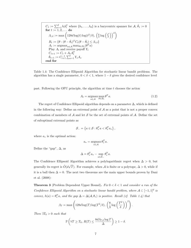
The state of the art result in this problem is due to Dani et al. (2008) who studied the

Confidence Ellipsoid Algorithm, shown here in Table 1.4. This algorithm (in a closed form)

was proposed, but not analyzed by Auer (2002). Dani et al. (2008) have shown that the

regret of this algorithm at time T is bounded by O(d√T ) 1. The algorithm implements the

OFU principle: it builds a high probability confidence set, Bt, around the true parameter

vector:

Bt = θ ∈ Rd | (θ − θt)TCt(θ − θt) ≤ βt

where βt = O(d log2 t), θt = argminθ∑ts=1(Ys − θTAs)2 is the least squares estimate of θ∗,

and where Ct =∑ts=1AsA

Ts is the correlation matrix built from the actions chosen in the

1We say that an = O(bn), where an ≥ 0, bn > 0 are two sequences if ∃m ≥ 0, C > 0 such thatan ≤ Cbn logm bn.

6

C1 :=∑di=1 bib

Ti where b1, . . . , bd is a barycentric spanner for A, θ1 := 0

for t := 1, 2, . . . do

βt,δ := max(

128d log(t) log(t2/δ),(

83 log

(t2

δ

))2)

Bt := θ : (θ − θt)TCt(θ − θt) ≤ βt,δAt := argmaxa∈Amaxθ∈Bt(θ

Ta)Play At and receive payoff YtCt+1 := Ct +AtA

Tt

θt+1 := C−1t+1

∑ts=1 YsAs

end for

Table 1.4: The Confidence Ellipsoid Algorithm for stochastic linear bandit problems. Thealgorithm has a single parameter, 0 < δ < 1, where 1− δ gives the desired confidence level

past. Following the OFU principle, the algorithm at time t chooses the action

At = argmaxa∈A

maxθ∈Bt

θTa. (1.2)

The regret of Confidence Ellipsoid algorithm depends on a parameter ∆, which is defined

in the following way: Define an extremal point of A as a point that is not a proper convex

combination of members of A and let S be the set of extremal points of A. Define the set

of suboptimal extremal points as

S− =a ∈ S : θT∗ a < θT∗ a∗

,

where a∗ is the optimal action:

a∗ = argmaxa∈A

θT∗ a.

Define the “gap”, ∆, as

∆ = θT∗ a∗ − supa∈S−

θT∗ a.

The Confidence Ellipsoid Algorithm achieves a polylogarithmic regret when ∆ > 0, but

generally its regret is O(d√T ). For example, when A is finite or a polytope, ∆ > 0, while if

it is a ball then ∆ = 0. The next two theorems are the main upper bounds proven by Dani

et al. (2008):

Theorem 3 (Problem Dependent Upper Bound). Fix 0 < δ < 1 and consider a run of the

Confidence Ellipsoid Algorithm on a stochastic linear bandit problem, where A ⊂ [−1, 1]d is

convex, h(a) = θT∗ a, and the gap ∆ = ∆(A, θ∗) is positive. Recall (cf. Table 1.4) that

βT = max

(128d log(T ) log(T 2/δ),

(83

log(T 2

δ

))2).

Then ∃T0 > 0 such that

P(∀T ≥ T0, R(T ) ≤ 8dβT,δ log T

∆

)≥ 1− δ.

7

Theorem 4 (Problem Independent Upper Bound). Consider the same setting as in Theo-

rem 3, except that ∆ = ∆(A, θ∗) > 0 is not required. Then ∃T0 > 0 such that

P(∀T ≥ T0, R(T ) ≤

√8d T βT,δ log T

)≥ 1− δ.

Dani et al. (2008) discuss the efficiency of the Confidence Ellipsoid Algorithm and point

out that the optimization problem (1.2) is NP-hard and so the Confidence Ellipsoid Algo-

rithm is not practical for large values of d. Dani et al. (2008) also propose another algorithm

that is computationally more efficient, but they only show a regret of O(d3/2√T ) for this

algorithm.

In addition to the above upper bounds, Dani et al. (2008) claim a lower bound of Ω(d√T )

2. This is for the case when supa∈A ‖a‖2 =√d. However, we believe that their lower bound

analysis seems to have a gap: The claim that the proof technique of Lemma 15 can be used

to prove Lemma 16 is not correct and Lemma 16 doesn’t hold as stated.

1.2.2 Associative Linear Bandits

Auer (2002) proposed the so-called SupLinRel algorithm for the adversarial Associative

Reinforcement Learning problem. In this problem at each time step t the learner has to

pick one of a finite number (K) of actions. However, before this choice an adversary is

presenting the d-dimensional side information vectors s1t, . . . , sKt to the learner. If the

learner chooses action i then he will receive a random payoff with mean θT∗ st, where θ∗ is an

unknown parameter vector. SupLinRel works by constructing a confidence ball for θ∗ and

uses the OFU principle to decide which action to choose, much like the Confidence Ellipsoid

Algorithm. The algorithm has a single parameter that should be chosen by the user.

Auer (2002) proves the following theorem (Theorem 6 in Auer (2002)):

Theorem 5. Let A = 1, . . . ,K. Assume that ‖θ∗‖2 ≤ 1 and rt ∈ [0, 1]. Fix 0 < δ < 1

and time T > 0. When algorithm SupLinRel is run with parameter δ/(1 + log T ) then with

probability 1− δ the regret of the algorithm up to time T is bounded by

R(T ) ≤ 44 [1 + log(2KT log(T/δ))]3/2√dT + 2

√T .

Note that the theorem in (Auer, 2002) has log T instead of log(T/δ), which is a mis-

print. It seems possible that SupLinRel can actually be used to simulate the behavior of a

Confidence Ellipsoid Algorithm (Auer, 2007). This opens up the possibility of an O(√dT )

regret bound for the class of problems satisfying the conditions stated in the theorem. Note

that here supa∈A ‖a‖2 = 1 and ‖θ‖2 ≤ 1. However, this construction is beyond the scope of

this thesis.2Let (an), (bn) be two nonnegative sequences. We say that an = Ω(bn) if ∃C > 0 such that an ≥ Cbn.

8

Inputs: T > 0 (horizon), 0 < ζ ≤ 1 (exponent in (1.3)).t := 1while t ≤ T do

n :=⌈(

tlog t

) 12ζ+1

⌉Initialize UCB1 with strategy set 1/n, 2/n, . . . , 1for s := t, t+ 1, . . . ,min(2t− 1, T ) do

Get action As from UCB1Play As and receive YtFeed Yt back to UCB1

end fort := 2t

end while

Table 1.5: CAB1 algorithm for continuum-armed bandit problems. Note that unlike theprevious algorithms, this algorithm needs to know the time horizon T > 0.

1.2.3 Continuum-armed Bandit Problems

In this section, we drop the linearity assumption of Section 1.2.1 and study the more general

case when the payoff function satisfies some smoothness conditions. This problem is called

the nonparametric or continuum-armed bandit problem.

Kleinberg (2004) considered the case when A = [0, 1]. He assumes that the target

function is uniformly locally Holder with constant L, exponent ζ ≤ 1, and neighborhood

size ν > 0 in the sense that for all a, a′ ∈ A with |a− a′| ≤ ν,

|h∗(a)− h∗(a′)| ≤ L |a− a′|ζ . (1.3)

Under this assumption, he proves a lower bound of O(Tζ+12ζ+1 ). He also proposes an algorithm,

CAB1, shown in Table 1.5, and proves the following theorem:

Theorem 6. For known ζ, the regret of algorithm CAB1 is O(Tζ+12ζ+1 log

ζ2ζ+1 (T )).

The idea behind CAB1 is simple, making this result very elegant: divide the action space into

appropriate number of intervals and play UCB1 on these intervals. However, the uniformly

locally Holderness assumption turns out to be quite restrictive: As Auer et al. (2007) point

out, if ζ > 1, h∗ must be a constant function.

Another related work is due to Cope (2006) who considered the case when the action

space is a convex compact subset of Rd. He assumes that the target function is unimodal,

three times differentiable, and it satisfies the inequalities

C1 ‖a− a∗‖22 ≤ (a− a∗)T[∂

∂aih∗(a)

]Di=1

,∥∥∥∥∥[∂

∂aih∗(a)

]Di=1

∥∥∥∥∥2

≤ C2 ‖a− a∗‖2 ,

9

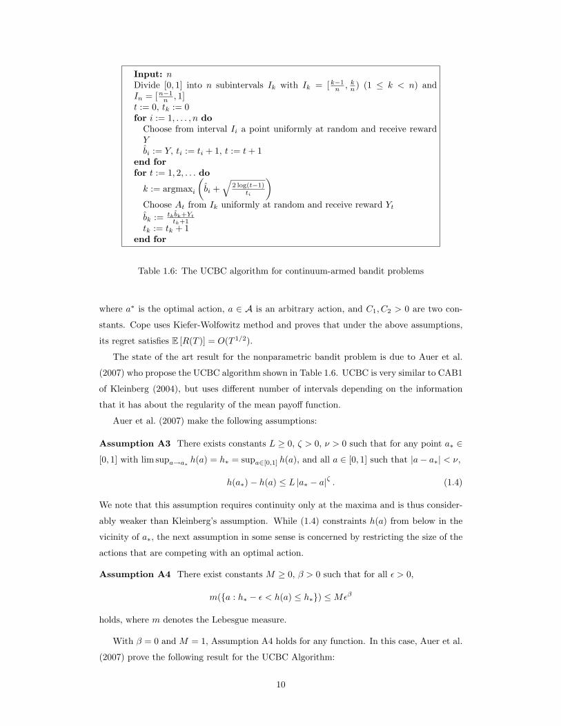
Input: nDivide [0, 1] into n subintervals Ik with Ik = [k−1

n , kn ) (1 ≤ k < n) andIn = [n−1

n , 1]t := 0, tk := 0for i := 1, . . . , n do

Choose from interval Ii a point uniformly at random and receive rewardYbi := Y, ti := ti + 1, t := t+ 1

end forfor t := 1, 2, . . . do

k := argmaxi

(bi +

√2 log(t−1)

ti

)Choose At from Ik uniformly at random and receive reward Ytbk := tk bk+Yt

tk+1tk := tk + 1

end for

Table 1.6: The UCBC algorithm for continuum-armed bandit problems

where a∗ is the optimal action, a ∈ A is an arbitrary action, and C1, C2 > 0 are two con-

stants. Cope uses Kiefer-Wolfowitz method and proves that under the above assumptions,

its regret satisfies E [R(T )] = O(T 1/2).

The state of the art result for the nonparametric bandit problem is due to Auer et al.

(2007) who propose the UCBC algorithm shown in Table 1.6. UCBC is very similar to CAB1

of Kleinberg (2004), but uses different number of intervals depending on the information

that it has about the regularity of the mean payoff function.

Auer et al. (2007) make the following assumptions:

Assumption A3 There exists constants L ≥ 0, ζ > 0, ν > 0 such that for any point a∗ ∈

[0, 1] with lim supa→a∗ h(a) = h∗ = supa∈[0,1] h(a), and all a ∈ [0, 1] such that |a− a∗| < ν,

h(a∗)− h(a) ≤ L |a∗ − a|ζ . (1.4)

We note that this assumption requires continuity only at the maxima and is thus consider-

ably weaker than Kleinberg’s assumption. While (1.4) constraints h(a) from below in the

vicinity of a∗, the next assumption in some sense is concerned by restricting the size of the

actions that are competing with an optimal action.

Assumption A4 There exist constants M ≥ 0, β > 0 such that for all ε > 0,

m(a : h∗ − ε < h(a) ≤ h∗) ≤Mεβ

holds, where m denotes the Lebesgue measure.

With β = 0 and M = 1, Assumption A4 holds for any function. In this case, Auer et al.

(2007) prove the following result for the UCBC Algorithm:

10

Theorem 7. Pick T > 0, n =(

Tlog T

) 12ζ+1

. Then

E [R(T )] ≤(

4L+c

LT

1+ζ1+2ζ (log T )

ζ1+2ζ

).

Further if n =(

Tlog T

) 13

and if T is sufficiently large, then

E [R(T )] ≤ 4LTmax1− ζ3 ,23(log T )

13 +

c

LT

23 (log T )

23 .

Note that the bound in the first part is generally tighter than the one in the second part.

However the first part requires the knowledge of ζ while the second doesn’t require this.

Auer et al. (2007) also prove that under Assumptions A3 and A4, for known ζ and β,

with n =(

Tlog T

) 11+2ζ−ζβ

, we get

E [R(T )] ≤(

4L+4cMLβ−1

21−β − 1

)T

1+ζ−ζβ1+2ζ−ζβ (log T )

ζ1+2ζ−ζβ ,

which is unimprovable (see Theorem 3 in Auer et al. (2007)). Finally, for an important

special case, Auer et al. (2007) prove the following theorem:

Theorem 8. If h has a finite number of maxima a∗ with lim supa→a∗ h(a) = h∗ and h

has continuous second derivatives which are non-vanishing at all these a∗ then UCBC with

n =(

Tlog T

) 14

achieves

E [R(T )] ≤ O(√T log T ).

11

Chapter 2

Playing in Parametric BanditProblems

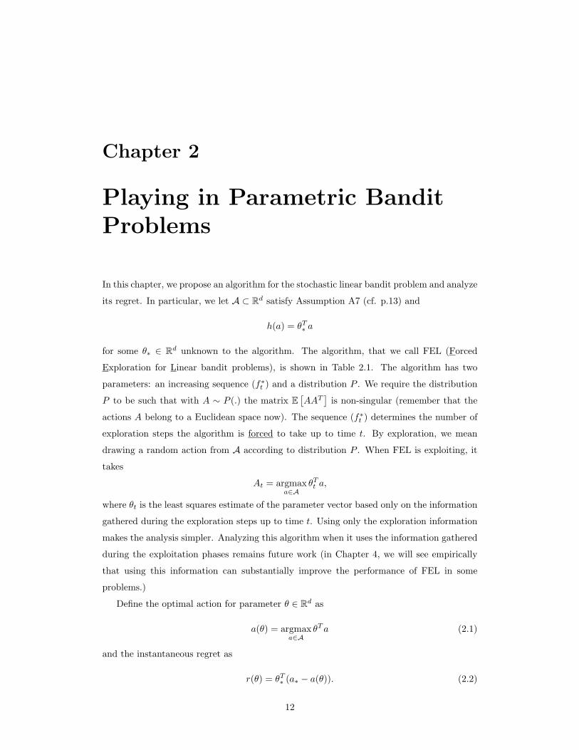
In this chapter, we propose an algorithm for the stochastic linear bandit problem and analyze

its regret. In particular, we let A ⊂ Rd satisfy Assumption A7 (cf. p.13) and

h(a) = θT∗ a

for some θ∗ ∈ Rd unknown to the algorithm. The algorithm, that we call FEL (Forced

Exploration for Linear bandit problems), is shown in Table 2.1. The algorithm has two

parameters: an increasing sequence (f∗t ) and a distribution P . We require the distribution

P to be such that with A ∼ P (.) the matrix E[AAT

]is non-singular (remember that the

actions A belong to a Euclidean space now). The sequence (f∗t ) determines the number of

exploration steps the algorithm is forced to take up to time t. By exploration, we mean

drawing a random action from A according to distribution P . When FEL is exploiting, it

takes

At = argmaxa∈A

θTt a,

where θt is the least squares estimate of the parameter vector based only on the information

gathered during the exploration steps up to time t. Using only the exploration information

makes the analysis simpler. Analyzing this algorithm when it uses the information gathered

during the exploitation phases remains future work (in Chapter 4, we will see empirically

that using this information can substantially improve the performance of FEL in some

problems.)

Define the optimal action for parameter θ ∈ Rd as

a(θ) = argmaxa∈A

θTa (2.1)

and the instantaneous regret as

r(θ) = θT∗ (a∗ − a(θ)). (2.2)

12

Let C0 := I, y0 := 0, θ0 := 0, f0 := 0 C0 ∈ Rd×d, and y0, θ0 ∈ Rdfor t := 1, 2, . . . do

if ft−1 < f∗t thenExploration:At ∼ P Draw a random action from A according to distribution PTake At and receive payoff YtCt := Ct−1 +AtA

Tt

yt := yt−1 + YtAtθt := (I + Ct)−1ytft := ft−1 + 1

elseExploitation:At := argmaxa∈A θTt−1aTake At and receive payoff YtCt := Ct−1, yt := yt−1, θt := θt−1, ft := ft−1

end ifend for

Table 2.1: FEL algorithm for stochastic linear bandit problems. Note that I denotes theidentity matrix, making the algorithm estimate the unknown parameter using ridge regres-sion. Note that ft, unlike Ct and θt, is not random.

The main idea of FEL and its regret analysis in Section 2.2 (cf. p.25) is that under various

conditions (cf. Section 2.3 on p.27) the following assumption holds:

Assumption A5 The regret function, as defined by (2.2), satisfies

r(θ) ≤ c ‖θ − θ∗‖22 + c′ ‖θ − θ∗‖32 ,

for some c, c′ > 0.

In Section 2.3, we will show that this assumption holds for a few interesting action spaces.

We also make the following assumptions:

Assumption A6 The probability distribution P is such that if A ∼ P (.) then the matrix

E[AAT

]is non-singular.

Assumption A7 There exists B > 0 such that for any a ∈ A, ‖a‖2 ≤ B.

This means that function r(θ) can be bounded from above by ‖θ − θ∗‖22 around θ∗. This

fact will be used in Section 2.2 to show that the regret of FEL with f∗t = d√t up to time T

is upper bounded by d√T + O

(√T

dν2d

), where νd is the smallest eigenvalue of the dispersion

matrix E[A1A

T1

].

2.1 Analysis of Least Squares Solution

Let θt be the estimate of θ∗ at time step t produced by the FEL algorithm, which is

essentially the ridge regression estimator. As said before we assume that r(θ) ≤ c ‖θ − θ∗‖22+

13

c′ ‖θ − θ∗‖32. So, given a bound on ‖θ − θ∗‖2, we can bound the instantaneous regret. In

this section, we provide such a bound for ‖θ − θ∗‖2. This result might be well-known in the

literature, though we were not able to find it. First we state our assumptions and then the

main theorem will be presented.

For the convenience of the reader we collect the most important quantities used in the

algorithm and in the proofs below in the following definition:

Definition 1. Let Cf and Cf,1, be constants such that for all t, 2∑di=1

(1 + 2

ftν2d

)2

≤ Cfd

and Cf,1f∗t ≤ ft. Let

Ht =t∑

s=1

Ifs−1≤f∗s AsZs,

Ct =t∑

s=1

Ifs−1≤f∗s AsATs , (unnormalized empirical dispersion matrix)

St =t∑

s=1

Ifs≤f∗s AsYs,

Ct = I + Ct,

θt = C−1t St (estimate of θ∗)

Further, let

Ct = UtΛtUTt

be the SVD decomposition of Ct, where

Λt = diag(λt1, . . . , λtd),

with λt1 ≥ · · · ≥ λtd and UtUTt = I. Finally, let

Dt = (Λt + I)−1Λt − I

and let ν1 ≥ . . . νd > 0 be the eigenvalues of the dispersion matrix E[A1A

T1

]. In what

follows, for a positive definite matrix C we let λmax(C) (λmin(C)) denote its maximum

(respectively minimum) eigenvalue.

Theorem 9. Let Assumptions A1, A2 (cf. p.6), A6 and A7 (cf. p.13) hold. Let θt, νd,

Cf , and Cf,1 be as defined by Definition 1. Let c1 = ν2d/(16d2) and

c2 =16(1 + log(4d))

(1 + νd/2)2 min1, 72d/ν2d.

Then for t big enough such that

f∗t ≥1

Cf,1max

2c1

(−(log c2 − 2 log t) + log

1c1

),

48d2

ν2d

(log

24d2

ν2d

− 13

log16d3 log(d(d+ 1))

ν4d

)it holds that

E[‖θt − θ∗‖22

]≤ 256(1 + log(4d))B2

Cf,1f∗t ν2d min1, 72d/ν2

d+ 2 ‖θ∗‖22

(Cfd

ν2dC

2f,1f

∗2t

+32d3 log ed(d+ 1)

C3f,1f

∗3t ν4

d

).

14

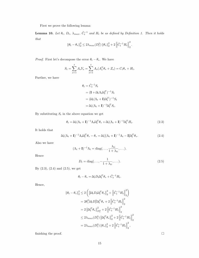
First we prove the following lemma:

Lemma 10. Let θt, Dt, λmax, C−1t and Ht be as defined by Definition 1. Then it holds

that

‖θt − θ∗‖22 ≤ 2λmax(D2t ) ‖θ∗‖

22 + 2

∥∥∥C−1t Ht

∥∥∥2

2.

Proof. First let’s decompose the error θt − θ∗. We have

St =t∑

s=1

AsYs =t∑

s=1

As(ATs θ∗ + Zs) = Ctθ∗ +Ht.

Further, we have

θt = C−1t St

= (I + UtΛtUTt )−1St

= (Ut(Λt + I)UTt )−1St

= Ut(Λt + I)−1UTt St.

By substituting St in the above equation we get

θt = Ut(Λt + I)−1ΛtUTt θ∗ + Ut(Λt + I)−1UTt Ht. (2.3)

It holds that

Ut(Λt + I)−1ΛtUTt θ∗ − θ∗ = Ut[(Λt + I)−1Λt − I]UTt θ∗. (2.4)

Also we have

(Λt + I)−1Λt = diag(. . . ,λti

1 + λti, . . . ).

Hence

Dt = diag(. . . ,− 11 + λti

, . . . ). (2.5)

By (2.3), (2.4) and (2.5), we get

θt − θ∗ = UtDtUTt θ∗ + C−1t Ht.

Hence,

‖θt − θ∗‖22 ≤ 2(∥∥UtDtUTt θ∗

∥∥2

2+∥∥∥C−1

t Ht

∥∥∥2

2

)= 2θT∗ UtD2

tUTt θ∗ + 2∥∥∥C−1

t Ht

∥∥∥2

2

= 2∥∥UTt θ∗∥∥2

D2t

+ 2∥∥∥C−1

t Ht

∥∥∥2

2

≤ 2λmax(D2t )∥∥UTt θ∗∥∥2

2+ 2

∥∥∥C−1t Ht

∥∥∥2

2

= 2λmax(D2t ) ‖θ∗‖

22 + 2

∥∥∥C−1t Ht

∥∥∥2

2,

finishing the proof.

15

Hence we can bound E[‖θt − θ∗‖22

]by bounding E

[λmax(D2

t )]

and E[∥∥∥C−1

t Ht

∥∥∥2

2

]. We

will bound E[λmax(D2

t )]

and E[∥∥∥C−1

t Ht

∥∥∥2

2

]in the following subsections. In particular,

Lemma 11 bounds E[∥∥∥C−1

t Ht

∥∥∥2

2

]and Lemma 19 bounds E

[λmax(D2

t )]

by appropriate

quantities, leading to the desired result.

2.1.1 Bounding E[∥∥∥C−1

t Ht

∥∥∥2

2

]The next lemma upper bounds E

[∥∥∥C−1t Ht

∥∥∥2

2

]:

Lemma 11. Let Assumptions A1, A2 (cf. p.6), A6 and A7 (cf. p.13) hold. Let Ht be as

defined by Definition 1. Let c1 = ν2d/(16d2) and

c2 =16(1 + log(4d))

(1 + νd/2)2 min1, 72d/ν2d.

Then for

f∗t ≥2

c1Cf,1

(−(log c2 − 2 log t) + log

1c1

),

we have

E[∥∥∥C−1

t Ht

∥∥∥2

2

]≤ 128B2(1 + log(4d))

ftν2d min

1, 72d

ν2d

.

Further, if

f∗t ≥1

Cf,1max

4(

2dνd

)2

log t,128B2

ν2d

(1 +

2d9

)log2 t

,

then ∥∥∥C−1t Ht

∥∥∥2

2≤ 1

4holds w.p. 1− 4d/t.

We upper bound E[∥∥∥C−1

t Ht

∥∥∥2

2

]in two steps. First we upper bound ‖Ht‖2 and then we

lower bound the eigenvalues of Ct.

Lemma 12. Let Assumptions A1 and A7 (cf. p.6, p.13) hold. Let 0 ≤ δ ≤ 1 and Ht be as

defined as in Definition 1. Then, for any t ≥ 1, 0 < δ < 1,

‖Ht‖2 ≤ 2B√ftx+

2√

2dB x3

. (2.6)

where x = log 2dδ .

Proof. Fix t ≥ 1, 0 < δ < 1 and let x = log(2d/δ). Fix 1 ≤ i ≤ d. Let Fs =

σ(A1, Y1, . . . , As, Ys) be the σ-algebra defined by the history up to time s. Applying Bern-

stein’s inequality (cf. Theorem 36, Appendix B) to (Ifs−1≤f∗s ZsAsi,Fs), we get that for

any Vti > 0, the probability that both

|Hti| ≥√

2Vtix+2Bx

3and

t∑s=1

E[(Ifs−1≤f∗s ZsAsi)

2|Fs−1

]≤ Vti (2.7)

16

hold is at most δ/d, Let σ2i = E

[A2si

]. Note that since ‖a‖2 ≤ B holds for any a ∈ A,

d∑i=1

σ2i = E

[d∑i=1

A2si

]≤ B2. (2.8)

Choose Vti = ftσ2i . Since

∑ts=1 Ifs−1≤f∗s = ft (

∑ts=1 Ifs−1≤f∗s is the number of times we

explored, and ft in the algorithm just counts the number of exploration steps),

t∑s=1

E[(Ifs−1≤f∗s ZsAsi)

2|Fs−1

]≤ Vti

holds w.p.1, thanks to the independence (Asi) and the boundedness of (Zs). Thus,

|Hti| ≥√

2Vtix+2Bx

3

holds with probability at most δ/d. Thus, outside of an event of probability at most δ,

|Hti| ≤√

2Vtix+2Bx

3

holds for all 1 ≤ i ≤ d. We continue the calculation on the event when all these inequalities

hold. Squaring both sides and using (|a|+ |b|)2 ≤ 2(a2 + b2) we get that

d∑i=1

H2ti ≤ 4ft

(d∑i=1

σ2i

)x+ 2d

(2Bx

3

)2

.

Using (2.8), we getd∑i=1

H2ti ≤ 4ftB2 x+ 2d

(2Bx

3

)2

.

Using√|a|+ |b| ≤

√|a|+

√|b|, we get

‖Ht‖2 ≤ 2B√ftx+

2√

2dB x3

,

which is the desired inequality.

Remark 13. If Zs is an i.i.d. sequence then using McDiarmid’s inequality (cf. Theorem 37,

Appendix B) it is possible to prove that for all 0 < δ < 1, t ≥ 1,

‖Ht‖2 ≤ B√

2ft log1δ, (2.9)

which is tighter than the above bound in three ways: instead of log(2d/δ) the bound has

log(1/δ) and (2.9) does not have the second term that we have in (2.6). Finally, the leading

constant in the McDiarmid-based bound is smaller by a factor of√

2.

We lower bound the eigenvalues of Ct by using a matrix perturbation result stated as

Corollary 4.10 in (Stewart and Sun, 1990). First let us define the following matrix norms

17

for a matrix M = [mij ]n,ki,j=1:

‖M‖1 = max1≤j≤k

n∑i=1

|mij |,

‖M‖∞ = max1≤i≤n

k∑j=1

|mij |, (2.10)

‖M‖2 = σ(M).

Here σ(M) denotes the largest singular value of M .

Theorem 14 (Stewart and Sun (1990), Corollary 4.10). Let M be a symmetric matrix with

eigenvalues ν1 ≥ ν2 ≥ . . . ≥ νd and M = M + E denote a symmetric perturbation of M

such that the eigenvalues of M are ν1 ≥ ν2 ≥ . . . ≥ νd. Then,

maxi|νi − νi| ≤ ‖E‖2.

Now, we lower bound the eigenvalues of the unnormalized empirical dispersion matrix.

Lemma 15. Let 0 < δ < 1. Let λt1 ≥ . . . λtd > 0 and ν1 ≥ . . . νd > 0 be as defined in

Definition 1. Then there exists a time t0 > 0 such that for any fixed t > t0, with probability

at least 1− δ,

maxi|ftνi − λi| ≤ d

√2ft log d(d+ 1)/δ.

Proof. Let Et = Ct − E [Ct] and let eij be the (i, j)-th element of Et. By the Hoeffding-

Azuma inequality (cf. Theorem 35, Appendix B), w.p. at least 1−δ, it holds simultaneously

for any 1 ≤ i, j ≤ d that

|ei,j | ≤√

2ft log d(d+ 1)/δ.

By Theorem 2.11 of (Stewart and Sun, 1990) we have

‖Et‖22 ≤ ‖Et‖1 ‖Et‖∞ ≤ (dmaxi,j|eij |)2.

Hence,

‖Et‖2 ≤ d√

2ft log d(d+ 1)/δ. (2.11)

By Theorem 14 and Inequality (2.11), we get

maxi|ftνi − λi| ≤ d

√2ft log d(d+ 1)/δ,

finishing the proof.

Lemma 16. Fix 0 < δ < 1 and let νi and λti be as defined in Definition 1. If t is such that

ft ≥ 2(

2dνi

)2

log(d(d+ 1)

δ

)then

λti ≥ft2νi

holds w.p. at least 1− δ.

18

Proof. From Lemma 15,

P(|λti − ftνi| ≤ d

√2ft log d(d+ 1)/δ, i = 1, . . . , d

)≥ 1− δ

holds for any t, 0 < δ < 1. In order to have λti ≥ ft2 νi, we only need the following inequality

to hold:

ftνi − d√

2ft log d(d+ 1)/δ ≥ ftνi2.

With a series of rearrangement we get that this inequality is equivalent to

ft ≥8d2

ν2i

log d(d+ 1)/δ,

thus proving the result.

We also need the following lemma:

Lemma 17. Fix a, b, c, C > 0. Let Z be a random variable such that (i) P (Z > b) = 0 and

(ii) for any ε ∈ [0, a], P (Z > ε) ≤ C exp(−cε). Then

E [Z] ≤ 1 + logCc

+ (b− a) exp(−ca).

Proof. We may assume that Z ≥ 0 since E [Z] ≤ E [max(Z, 0)] and P (max(Z, 0) > ε) ≤

P (Z > ε). Then

E [Z] =∫ ∞

0

P (Z > ε) dε

≤∫ x

0

1dε+ Ix<aC∫ a

x

exp(−cε)dε+∫ b

a

C exp(−ca)dε

≤ x+ Ix<aC∫ ∞x

exp(−cε)dε+ C(b− a) exp(−ca)

= x+ Ix<aC exp(−cx)

c+ C(b− a) exp(−ca)

≤ 1 + logCc

+ C(b− a) exp(−ca),

where the last inequality follows from the choice x = log(C)/c.

Now, we are ready to upper bound E[∥∥∥C−1

t Ht

∥∥∥2

2

].

Proof of Lemma 11. Fix 0 < δ < 1 and let δ′ = δ/2. By Lemma 16, with probability at

least 1− δ′ it holds that λtd ≥ ftνd/2 ≥ 0 when

ft ≥ 2(

2dνd

)2

log(d(d+ 1)

δ′

). (2.12)

By Lemma 12, with probability 1− δ′,

‖Ht‖2 ≤ 2B

√ft log

4dδ

+2√

2dB3

log4dδ. (2.13)

19

Hence, since∥∥∥C−1

t Ht

∥∥∥2≤ λmax(C−1

t ) ‖Ht‖2 = λmin(Ct)−1 ‖Ht‖2, and λmin(Ctd) = 1+λtd,

we get from (2.13) that

∥∥∥C−1t Ht

∥∥∥2≤ 2B

1 + ftνd/2

(√ft log

4dδ

+

√2d3

log4dδ

)(2.14)

≤ 4B1 + ftνd/2

max

√ft log

4dδ,

√2d3

log4dδ

holds w.p. 1− δ when (2.12) holds. Let x =√

log(4d/δ). Hence∥∥∥C−1t Ht

∥∥∥2

2(4B

1+ftνd/2

)2 ≤ maxx2ft, x

4

(2d9

)(2.15)

holds w.p. 1− 4d exp(−x2) when

ft ≥ 4(

2dνd

)2

x2. (2.16)

Now, we apply Lemma 17 to bound the expected value of Z =∥∥∥C−1

t Ht

∥∥∥2

2/(

4B1+ftνd/2

)2

.

Lemma 17 requires a deterministic upper bound for Z. This is obtained as follows:∥∥∥C−1t Ht

∥∥∥2≤‖Ht‖21 + λdt

≤ ‖Ht‖2 ≤ Bt. (2.17)

Hence,

Z ≤ t2(1 + ftνd/2)2

16= b. (2.18)

Let

ε = maxx2ft, x4(2d/9),

a =f2t ν

2d

16d2a0, where a0 = max

1,

ν2d

72d

.

We show that if ε ≤ a, then Inequality (2.16) holds. Assume ε ≤ a. If a0 = 1, then

it follows from definition of ε that x2ft ≤ f2t ν

2d/(16d2), which gives Inequality (2.16). If

a0 = ν2d/(72d), then it follows from definition of ε that x4(2d/9) ≤ (f2

t ν4d)/((27)(32)d3),

which gives Inequality (2.16). Hence, by (2.15) and (2.16), if ε ≤ a then

P (Z > ε) ≤ 4d exp(−x2).

Next, we need to find C and c such that 4de−x2 ≤ Ce−cε. Using C = 4d, we get that this

is equivalent to x2 ≥ cε. This last inequality is satisfied if we had x2 ≥ cmaxx2ft, x

4(

2d9

),

or if x2 ≥ cx2ft and x2 ≥ cx4(2d/9). After rearrangements, using (2.16), we get that the

choice c = 1ft

min

1, 72dν2d

makes these inequalities true. Hence we have the following values

20

to be used in Lemma 17:

C = 4d,

a =f2t ν

2d

16d2max

1,

ν2d

72d

,

b =t2(1 + ftνd/2)2

16,

c =1ft

min

1,72dν2d

.

Now, by Lemma 17, we get the following upper bound for Z =∥∥∥C−1

t Ht

∥∥∥2

2/(

4B1+ftνd/2

)2

:

E

∥∥∥C−1

t Ht

∥∥∥2

2(4B

1+ftνd/2

)2

≤ 1 + logCc

+ (b− a) exp(−ca) ≤ 1 + logCc

+ b exp(−ca).

We have that exp(−ca) = exp(− ν2

d

16d2 ft

). Let c1 = ν2

d/(16d2) and

c2 =16(1 + log(4d))

(1 + νd/2)2 min1, 72d/ν2d.

By Proposition 33, if

ft ≥2c1

(−(log c2 − 2 log t) + log

1c1

). (2.19)

then b exp(−ca) ≤ 1+logCc . Hence under Condition (2.19), we have that

E[∥∥∥C−1

t Ht

∥∥∥2

2

]≤ 128B2(1 + log(4d))

ftν2d min

1, 72d

ν2d

,

proving the first part of the theorem.

Now we bound P(∥∥∥C−1

t Ht

∥∥∥2

2≤ 1/4

). Recall that we defined x =

√log(4d/δ). Choose

δ > 0 such that exp(−x2) = 1/t. Hence, x =√

log t. Hence, by (2.14),∥∥∥C−1t Ht

∥∥∥2

2

2(

2B1+ftνd/2

)2 ≤ ft log t+(

2d9

)log2 t

holds w.p. 1− 4d/t when

ft ≥ 4(

2dνd

)2

log t.

By Proposition 33, we can show that if

ft ≥128B2

ν2d

(1 +

2d9

)log2 t (2.20)

then

2(ft log t+

2d9

log2 t

)16B2

f2t ν

2d

≤ 14.

Hence, if Inequality (2.20) holds, then∥∥∥C−1t Ht

∥∥∥2

2≤ 1

4

holds w.p. 1− 4d/t.

21

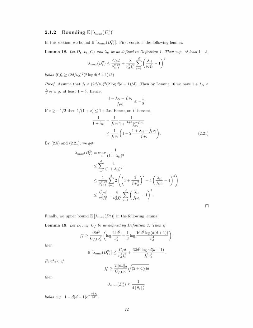
2.1.2 Bounding E [λmax(D2t )]

In this section, we bound E[λmax(D2

t )]. First consider the following lemma:

Lemma 18. Let Dt, νi, Cf and λti be as defined in Definition 1. Then w.p. at least 1− δ,

λmax(D2t ) ≤

Cfd

ν2df

2t

+8

ν2df

2t

d∑i=1

(λtiνift

− 1)2

holds if ft ≥ (2d/νd)2(2 log d(d+ 1)/δ).

Proof. Assume that ft ≥ (2d/νd)2(2 log d(d+ 1)/δ). Then by Lemma 16 we have 1 + λti ≥ft2 νi w.p. at least 1− δ. Hence,

1 + λti − ftνiftνi

≥ −12.

If x ≥ −1/2 then 1/(1 + x) ≤ 1 + 2x. Hence, on this event,

11 + λti

=1ftνi

11 + 1+λti−ftνi

ftνi

≤ 1ftνi

(1 + 2

1 + λti − ftνiftνi

). (2.21)

By (2.5) and (2.21), we get

λmax(D2t ) = max

i

1(1 + λti)2

≤d∑i=1

1(1 + λti)2

≤ 1ν2df

2t

d∑i=1

2

((1 +

2ftν2

d

)2

+ 4(λtiftνi

− 1)2)

≤ Cfd

ν2df

2t

+8

ν2df

2t

d∑i=1

(λtiftνi

− 1)2

.

Finally, we upper bound E[λmax(D2

t )]

in the following lemma:

Lemma 19. Let Dt, νd, Cf be as defined by Definition 1. Then if

f∗t ≥48d2

Cf,1ν2d

(log

24d2

ν2d

− 13

log16d3 log(d(d+ 1))

ν4d

),

then

E[λmax(D2

t )]≤ Cfd

ν2df

2t

+32d3 log ed(d+ 1)

f3t ν

4d

.

Further, if

f∗t ≥2 ‖θ∗‖2Cf,1νd

√(2 + Cf )d

then

λmax(D2t ) ≤

14 ‖θ∗‖22

holds w.p. 1− d(d+ 1)e−ν2dft8d2 .

22

Proof. Define Lt = ν2df

2t

8

(λmax(D2

t )−Cfd

ν2df

2t

)and Ft =

∑di=1

(d√

2ftftνi

)2

. Hence,

Lt ≤d∑i=1

(λtiftνi

− 1)2

(Lemma 18)

≤ log(d(d+ 1)

δ

) d∑i=1

(d√

2ftftνi

)2

(Lemma 15)

≤ Ft log(d(d+ 1)

δ

)holds w.p. at least 1− δ if

ft ≥ 2(

2dνd

)2

logd(d+ 1)

δ.

Note that here we used that Lemma 18 holds on the event set where the conclusion of

Lemma 15 holds. Substitute ε = log(d(d+ 1)/δ). Hence if

ε ≤ ν2dft

8d2(2.22)

then

P (Lt > Ftε) ≤ d(d+ 1) exp(−ε), (2.23)

or P (Lt > u) ≤ d(d+ 1) exp(− uFt

) if uFt≤ ν2

dft8d2 .

Now we want to apply Lemma 17 for Lt to bound its expected value from the above high

probability bound. Since Lemma 17 requires Lt to be deterministically upper bounded, we

now demonstrate such a bound. We have

λmax(D2t ) = max

i

1(1 + λti)2

=1

(1 + mini λti)2≤ 1.

Hence,

Lt ≤ν2df

2t

8− Cfd

8≤ ν2

df2t

8. (2.24)

Now by (2.22), (2.23) and (2.24), we obtain the following values to be used in Lemma 17:

C = d(d+ 1), c =1Ft, a =

Ftν2dft

8d2, b =

ν2df

2t

8.

Hence,

E [Lt] ≤1 + logC

c+ (b− a) exp(−ca)

≤ 1 + log(d(d+ 1))(1/Ft)

+ν2df

2t

8exp

(−ν

2dft

8d2

).

Let1 + log(d(d+ 1))

(1/Ft)≥ ν2

df2t

8exp

(−ν

2dft

8d2

).

23

By Proposition 33, this inequality holds when

ft ≥48d2

ν2d

(log

24d2

ν2d

− 13

log16d3 log(d(d+ 1))

ν4d

).

Hence we have seen that if t is big enough then

E [Lt] ≤ 2Ft log ed(d+ 1),

where

Ft =2d2

ft

d∑i=1

1ν2i

≤ 2d3

ftν2d

.

Hence

E [Lt] = E[ν2df

2t

8

(λmax(D2

t )−Cfd

ν2df

2t

)]≤ 4d3 log ed(d+ 1)

ftν2d

.

Reorder the above equation to get

E[λmax(D2

t )]≤ 8ν2df

2t

[4d3 log ed(d+ 1)

ftν2d

]+Cfd

ν2df

2t

=Cfd

ν2df

2t

+32d3 log ed(d+ 1)

f3t ν

4d

.

Now we prove the second part of the lemma. We know that if u ≤ ν2dftFt/(8d

2), then

P (Lt < u) ≥ 1− d(d+ 1) exp(− u

Ft

).

Let u = ν2dftFt/(8d

2). Hence,

P(Lt <

ν2dftFt8d2

)≥ 1− d(d+ 1)e−

ν2dft8d2 .

Hence,

λmax(D2t ) ≤

1ν2df

2t

(ν2dftFtd2

+ Cfd

)holds w.p. at least 1− d(d+ 1)e−

ν2dft8d2 . Now notice that if

ft ≥2 ‖θ∗‖2νd

√(2 + Cf )d

then

λmax(D2t ) ≤

14 ‖θ∗‖22

holds w.p. 1− d(d+ 1)e−ν2dft8d2 .

2.1.3 Putting all together

Proof of Theorem 9. By Lemmas 10, 11 and 19, we get

E[∥∥∥θ − θ∗∥∥∥2

2

]≤ 2E

[λmax(D2

t )]‖θ∗‖22 + 2E

[∥∥∥C−1t Ht

∥∥∥2

2

]≤ 256(1 + log(4d))B2

ftν2d min1, 72d/ν2

d+ 2 ‖θ∗‖22

(Cfd

ν2df

2t

+32d3 log ed(d+ 1)

f3t ν

4d

).

Using Cf,1f∗t ≤ ft gives the desired result.

24

Remark 20. Assume that B = 1 and that νd behaves like 1/d. This makes the bound of

Theorem 9 in the order of O(d/√t). We show that this is the best upper bound that we can

achieve by using the least squares solution (the same applies to ridge regression). Assume

action space is A = e1, . . . , ed, where ei is the ith unit vector. Then it is easy to see that

the least squares solution satisfies E[‖θt − θ∗‖22

]≈ d2σ2/f∗t , where σ2 is the variance of the

noise. Then use the exploration rate of f∗t = d√t and get E

[‖θt − θ∗‖22

]= dσ2/

√t.

2.2 FEL Analysis

First, we prove the following lemma:

Lemma 21. Let Assumptions A2 and A5 hold. Then it holds that

E [r(θt)] ≤ E[(c+ c′) ‖θt − θ∗‖22

]+ 2P

(‖θt − θ∗‖22 ≥ 1

).

Proof. By Assumption A5 (cf. p.13),

r(θt) ≤ c ‖θt − θ∗‖22 + c′ ‖θt − θ∗‖32 .

(2.25)

Let Zt = ‖θt − θ∗‖2. Because r(θt) ≤ 2, we have that

r(θt) ≤ min2, cZ2 + c′Z3.

Hence,

E [r(θ)] ≤ E[min2, cZ2 + c′Z3

]= P

(Z2 < 1

)E[min2, cZ2 + c′Z3|z2 < 1

]+ P

(Z2 ≥ 1

)E[min2, cZ2 + c′Z3|Z2 ≥ 1

]≤ P

(Z2 < 1

)E[min2, (c+ c′)Z2|Z2 < 1

]+ P

(Z2 ≥ 1

)E[min2, (c+ c′)Z3|Z2 ≥ 1

]≤ P

(Z2 < 1

)E[min2, (c+ c′)Z2|Z2 < 1

]+ 2P

(Z2 ≥ 1

)≤ P

(Z2 < 1

)E[(c+ c′)Z2|Z2 < 1

]+ 2P

(Z2 ≥ 1

)≤ E

[(c+ c′)Z2

]+ 2P

(Z2 ≥ 1

).

The main result of our analysis is the following theorem:

Theorem 22. Let Assumptions A1, A2 (cf. p.6), A5, A6 and A7 (cf. p.13) hold. Let

25

νd > 0 be the smallest eigenvalue of E[A1A

T1

]. Let

G1 =256(1 + log(4d))B2

Cf,1d ν2d min

1, 72d

ν2d

,G2 =

4Cfd ‖θ∗‖22C2f,1d

2ν2d

,

G3 =64 log(ed(d+ 1)) ‖θ∗‖22

C3f,1ν

4d

.

Further let c1 = ν2d/(16d2) and

c2 =16(1 + log(4d))

(1 + νd/2)2 min1, 72d/ν2d.

Let

f∗t ≥1

Cf,1max

2c1

(−(log c2 − 2 log t) + log

1c1

), 4(

2dνd

)2

log t,128B2

ν2d

(1 +

2d9

)log2 t,

(2.26)

48d2

ν2d

(log

24d2

ν2d

− 13

log16d3 log(d(d+ 1))

ν4d

),

2 ‖θ∗‖2νd

√(2 + Cf )d,

8d2

ν2d

(log t− log

4d+ 1

).

Finally, let c and c′ be the constants of Assumption A5. Then the expected regret of FEL

with f∗t = d√t up to time T satisfies

E [R(T )] ≤ fT + t1 + 16d log T + 1 + (c+ c′)[2G1

√T +G2 +G2 log T + 2G3

].

Proof. By Theorem 9, for t ≥ t1, it holds that

E[‖θt − θ∗‖22

]≤ 256(1 + log(4d))B2

Cf,1f∗t ν2d min1, 72d/ν2

d+ 2 ‖θ∗‖22

(Cfd

ν2dC

2f,1f

∗2t

+32d3 log ed(d+ 1)

C3f,1f

∗3t ν4

d

).

(2.27)

By Lemma 21, we have that

E [r(θt)] ≤ E[(c+ c′) ‖θt − θ∗‖22

]+ 2P

(‖θt − θ∗‖22 ≥ 1

). (2.28)

Let X1 = 2λmax(D2t ) ‖θ∗‖

22, X2 = 2

∥∥∥C−1t Ht

∥∥∥2

2and Z = ‖θt − θ∗‖2. By Lemma 10, we have

that

Z2 ≤ X1 +X2.

We have that

Z2 ≥ 1 ⊂ X1 +X2 ≥ 1 ⊂X1 ≥

12

∪X2 ≥

12

.

Hence, by the second parts of Lemmas 11 and 19,

P(Z2 ≥ 1

)≤ P

(X1 ≥

12

)+ P

(X2 ≥

12

)≤ 4d

t+ d(d+ 1) exp

(−ν

2dft

8d2

).

26

Hence,

E [r(θt)] ≤ (c+ c′)E[‖θt − θ∗‖22

]+

4dt

+ d(d+ 1) exp(−ν

2dft

8d2

)≤ (c+ c′)E

[‖θt − θ∗‖22

]+

8dt. (2.29)

The last step holds when

ft ≥8d2

ν2d

(log t− log

4d+ 1

).

Inequality (2.29), (2.28) and (2.27) gives that

E [r(θt)] ≤ (c+ c′)

(256(1 + log(4d))B2

Cf,1f∗t ν2d min1, 72d/ν2

d+ 2 ‖θ∗‖22

(Cfd

ν2dC

2f,1f

∗2t

+32d3 log d(d+ 1)

C3f,1f

∗3t ν4

d

))+

16dt

≤ (c+ c′)[G1d

f∗t+G2d

2

f∗2t+G3d

3

f∗3t

]+

16dt.

By the choice of f∗t = d√t, we get the final result as follows:

E [R(T )] ≤T∑t=1

(Ift<f∗t + (1− Ift<f∗t )E [rt])

≤ fT +T∑t=1

(1− Ift<f∗t )E [r(θt)]

≤ fT +T∑t=1

E [r(θt)]

≤ fT + t1 + 16d log T + 1 + (c+ c′)[2G1

√T +G2 +G2 log T + 2G3

].

In the second line above we used that in a time step when FEL is exploiting, rt = r(θt).

Remark 23. After hours and hours of tedious calculations using Proposition 33 several times

one can show that if

t ≥ max

(16

cCf,1d

)2(14

log1c1c2

+ log8

cCf,1d

),

(16d

ν2dCf,1

)2

,

(64B

√2 + 4d/9

νd√dCf,1

log32B

√2 + 4d/9

νd√dCf,1

)4

,

(48dν2d

)2(log

24d2

ν2d

− 13

log16d3 log(d(d+ 1))

ν4d

)2

,

4 ‖θ∗‖22 (2 + Cf )dν2d

,

(32dν2d

)2(−1

2log

4d+ 1

+ log16dν2d

),

then condition (2.26) is satisfied.

2.3 Results For Various Action Sets

In this section, we consider some cases when the action set A is such that the regret function

will satisfy Assumption A5 (cf. p.13).

27

Strictly convex action sets

Let us assume that the action set is the 0-level set of some strictly convex, sufficiently

smooth function, c : Rd → R:

A = a ∈ Rd : c(a) ≤ 0 . (2.30)

Note that a(θ) is the solution of the following constrained, parametric linear optimization

problem:

−θTa→ min (2.31)

s.t. c(a) ≤ 0.

Since the linear objective function is unbounded on Rd, the solution always lies on the

boundary of the set A, i.e., c(a(θ)) = 0 holds for any θ. We make the following assumption:

Assumption A8 The function c is four-times differentiable in a neighborhood of θ∗ and

if λ(θ) denotes the the Langrange multiplier underlying the solution of the optimization

problem (2.31) when the parameter is θ then λ(θ) is differentiable in the same neighborhood1.

Then with the help of the Karush-Kuhn-Tucker (KKT) Theorem (cf. Theorem 32, Ap-

pendix A) and the Implicit Function Theorem (cf. Theorem 31, Appendix A) one gets

that

−θ + λ(θ)Dac(a(θ)) = 0.

If we take derivative with respect to θ and reorder the result, we get that

Dθa(θ) = − 1λ(θ)

(D2ac(a(θ)))−1 (Dac(a(θ))Dθλ(θ) + I) ,

where Dz is the derivative operator with respect to argument z.2 It also follows from this

argument that if the fourth order partial derivatives of c exist and are continuous then a(·)

is three times differentiable.

Let f(a; θ) = −θTa. Note that r(θ) = θT∗ a∗ − f(a(θ); θ∗). We want to show that

Dθf(a(θ); θ∗)∣∣θ=θ∗

= 0. Using the chain rule,

Dθf(a(θ); θ∗) = Daf(a(θ); θ∗)Dθa(θ).

By the KKT conditions,

Daf(a(θ∗); θ∗) = λ(θ∗)Dac(a(θ∗)).

Further, by the complementary condition of the KKT theorem, λ(θ)c(a(θ)) = 0. Hence,

0 = Dθ(λ(θ∗)c(a(θ∗))) = c(a(θ∗))Dθλ(θ∗) + λ(θ∗)Dθc(a(θ∗)) = λ(θ∗)Dθc(a(θ∗))1Note that the differentiability of λ could be proven using arguments like in Chapter 12 of Nocedal and

Wright (2006). These proofs are considerably technical and go beyond the scope of this thesis.2That λ(θ) > 0 follows from the KKT Theorem.

28

since c(a(θ∗)) = 0. Hence,

Dθf(a(θ); θ∗)∣∣θ=θ∗

= λ(θ∗)Dac(a(θ∗))Dθa(θ∗) = λ(θ∗)Dθc(a(θ∗)) = 0.

Resorting to the Taylor-series expansion of r(θ), we get the following result:

Theorem 24. Assume that the action set is given by (2.30), where c is a function that

is strictly convex. Further, let Assumption A8 (cf. p.28) hold. Then the regret function r

satisfies Assumption A5 (cf. p.13).

Note that if A is a sphere, or more generally an ellipsoid then A will satisfy the conditions

of this theorem. In particular, when A is the unit sphere and the length of θ∗ is one,

r(θ) = ‖(θ/ ‖θ‖2)− θ∗‖22, which can be used to show that in Assumption A5 (cf. p.13) in

this case c = 1 can be chosen to be independent of d.

We suspect that the above result holds for very general action sets. In particular, it

is not very difficult to see that the statement continues to hold when the set is described

by a number of convex constraints which are all active in a neighborhood of a∗, such as in

the example constructed for the lower bound proof in (Dani et al., 2008). One may believe

based on the proof of this result that smoothness of a(·) is important. In the next section,

we will look at the case when a(·) can have jumps, showing that smoothness is not essential.

However, it remains for future work to fully characterize the cases when the subquadratic

growth of r holds.

Polytopes

In this section we assume that the action set A is a polytope (an intersection of a finite

number of half-spaces). In this case without the loss of generality one can define function

a(·) such that its range is the vertex set of the polytope. Then r(θ∗) becomes a piecewise

constant function. We want to show that it is constant in a small neighborhood of θ∗. Let

F be the unique i-face of the polygon for the largest i = 0, 1, . . . , d− 1 that contains a(θ∗)

and which is perpendicular to θ∗. (If there is no such i-face with i ≥ 1 then we take F to be

the vertex a(θ∗).) By an elementary argument it follows that there exist a neighborhood U

of θ∗ such that if θ ∈ U then a(θ) is on F . Since F is perpendicular to θ∗, for any a, a′ ∈ F ,

θT∗ a = θT∗ a′. Hence, we have the following result:

Theorem 25. Assume that A is a polytope. Then the regret function r is zero in a neigh-

borhood of θ∗ and thus satisfies Assumption A5 (cf. p.13).

Note that if the action set is a polytope, the forcing schedule can be changed to e.g.

ft = c log2(t), which by an argument similar to the above one, but which exploits that the

regret function is constant in a small neighborhood of θ∗, gives a regret bound of order

O(c log2 T ) (the probability of choosing a suboptimal vertex in the exploitation step will

29

decay at least as fast 1/T , while the exploration steps contribute to the log2 T growth of the

regret). Note that in order to optimize the scaling of the regret with the dimension d, one

should choose c to be proportional to√d. Clearly, with this approach any regret slightly

faster than log(t) can be achieved at the price of increasing the transient period.

2.3.1 Generalized Linear Payoff

Now, assume that the reward function takes the form: h(a; θ) = θTφ(a), i.e., the reward

function takes the form of a generalized linear function (the function is linear in the param-

eters, but not in the actions). Here φ : A → Rd and now the action space does not need to

be a subset of a Euclidean space (or it could be a subset of a Euclidean space of dimension,

say s 6= d). This case is interesting from the point of view of practical applications where the

expected relatedness of the actions can be expressed with the help of some features φ (e.g.,

the actions could be grouped based on their expected similarity which can be expressed via

the help of features; see Section 4.)

In order to make a connection to the linear payoff case, assume that the decision

maker chooses a random action A from some distribution P. Then the expected im-

mediate reward of this random action is E [h(A; θ)] = θTE [a]. If P =∑k pkδak then

E [h(A; θ)] = θT∑k pkφ(ak). Hence, if one defines A as the convex hull of A then we

can view the problem as one defined with action set A and with a linear reward function

h(a; θ) = θT a. Thus, we can apply Algorithm 2.1 to this problem. Note that the optimiza-

tion problem argmaxa∈A θT a will have solutions on the boundary of A. This means that in

the exploitation steps, the algorithm can always select a non-randomized action.

If the action set A is finite, A becomes a polytope in which case the associated regret

function satisfies Assumption A5 (cf. p.13). More generally, if this growth condition is

satisfied, the algorithm’s regret will be of order d√T in time T , where d is the dimension of

the parameter space. Thus, the dimension (or cardinality) of the action space does not play

a direct role in the regret of the algorithm (as expected). (Of course, these remarks apply

to any linear bandit algorithm whose regret can be bounded in terms of the dimension of

the parameter space.)

30

Chapter 3

Non-parametric Bandits

In this section, we drop the linearity assumption of Chapter 2 and study the more general

case when the payoff function satisfies some smoothness conditions but is otherwise unre-

stricted. In particular, no parametric form for the payoff function is assumed, hence we call

this the non-parametric case.

Table 3.1 shows the FEC Algorithm (Forced Exploration for Continuum-armed bandit

problems), which is a modified version of the FEL Algorithm of Chapter 2. The main ideas

are (i) using d∗t basis functions to estimate h∗; (ii) gradually increasing d∗t over time; (iii)

and using a deterministic schedule for the exploration. The advantage of this algorithm

is that it allows a flexible combination of known payoff structures with a non-parametric

approach. In the next section we show that the regret of FEC at time T satisfies E [R(T )] =

O(T2+α2+2α ) assuming that the mean payoff function is (in some sense that will be made

precise) smooth up to order α. Unfortunately, this bound is not as good as the bound for

UCBC shown in Theorem 7. In particular, for ζ = α, the difference between the exponents

is α/((2+2α)(1+2α)). Thus, although the exponent that we get for the regret is larger than

the exponent for UCBC, the difference becomes negligible as α gets large. The difference is

the result that in the parametric case our algorithm has a regret of order O(d√T ) instead

of O(√dT ).

3.1 FEC Analysis

In this section, we analyze the regret of FEC. Let D > 0 and d > 0 be integers. Let Pd,D be

the class of all polynomials on domain A ⊂ RD whose coordinatewise degree does not exceed

d, φd : A → [−1, 1]d be the basis functions that spans Pd,D. Let (dt) be an appropriate

increasing sequence of integers and, by slightly abusing the notation, let us abbreviate φdtwith φt. Further, let

h∗t = θTt φt (3.1)

31

Input: A sequence of bases functions: B = b1, b2, . . . ,where bd : A → [−1, 1]d, sequences (f∗t ), (d∗t ), distributions (Pd)

Initialization: Let f0 := 0, d0 = 1, C0 := 0, y0 := 0, θ0 := 0C0 ∈ Rd0×d0 , and y0, θ0 ∈ Rd0

for t := 1, 2, . . . doif ft−1 < f∗t thenExploration:At ∼ Pdt Draw a random action from A according to distribution PdtTake At and observe YtCt := Ct−1 + φt(At)φt(At)T

yt := yt−1 + Ytφt(At)θt := (I + Ct)−1ytft := ft−1 + 1

elseExploitation:At := argmaxa∈A θTt−1φt(a)Take At and receive payoff YtCt := Ct−1, yt := yt−1, θt := θt−1, ft := ft−1

end ifif dt−1 < d∗t thenChanging to a new basis:dt := d∗tφt := bdtReset Ct, yt, θt:Ct :=

∑ts=1 φt(As)φt(As)

T

yt :=∑ts=1 Ysφt(As)

θt := (I + Ct)−1ytelsedt := dt−1

end ifend for

Table 3.1: FEC algorithm for continuum-armed bandit problems. Note that if bd+1 is anextension of bd then the resetting of Ct, yt, θt can be done in an efficient manner.

32

be the closest point to h∗ in Pdt,D with respect to the supremum norm1,

h∗t = argminh∈Pdt,D

‖h∗ − h‖∞ , (3.2)

which, for the sake of simplicity, we will assume to exist. Further, let

Ψt = supa∈A‖φt(a)‖2 ,

ζt =∥∥∥θt∥∥∥

2.

Define the instantaneous regret as

r∗t = h∗(a∗)− h∗(At)

and the instantaneous regret with respect to h∗t as

rt = h∗t (a∗t )− h∗t (At),

where a∗t = argmaxa∈A h∗t (a) and At is the action chosen by FEC at time t (to be defined

below). Further, define

rt(θ) = h∗t (a∗t )− h∗t (at(θ)),

where at(θ) = argmaxa∈A θTφt(a). Define the vector norms ‖v‖2 =√∑

i v2i , ‖v‖∞ =

maxi |vi| and function norms ‖f‖2 =√∫A f

2(a)da, ‖f‖∞ = supa∈A |f(a)|. It is easy to see

that ‖v‖∞ ≤ ‖v‖2 and ‖f‖2 ≤ ‖f‖∞.

We make the following assumptions:

Assumption A9 The target function h∗ is a member of the Sobolev space Wα(L∞(A))

(cf. Definition 5, Appendix A).

Assumption A10 Let θt be as defined in (3.1) and (3.2). The instantaneous regret with

respect to h∗t satisfies

rt(θ) ≤ c∥∥∥θ − θt∥∥∥2

2+ c′

∥∥∥θ − θt∥∥∥3

2,

where c, c′ > 0 are some constants.

Assumption A11 The distributions (Pd) are such that if νd is the minimum eigenvalue

of E[AAT

], where A ∼ Pd then, H/d ≤ νd ≤ J for some constants H and J .

Assumption A12 We have that Ψt ≤ 1 and ζt ≤√dt.

In order to prove the main result of this chapter, we need the following theorem. The

theorem is stated in the form given here as Theorem 2.3 in (French et al., 2003).

1Also known as the “best approximation” of h∗ in Pdt,D.

33

Theorem 26 (Jackson’s theorem). Let 1 ≤ p ≤ ∞ and α ≥ 1 be integers. Given h ∈

Wα(Lp([−1, 1]D)), there exists a constant E > 0 such that for all integers D, d ≥ 1, there

exists a polynomial P ∈ Pd,D such that

‖h− P‖p ≤ E(d+ 1)−α ‖h‖p .

Next, we define some constants and functions:

Definition 2. Let

γ =α+ 22α+ 2

, β =1

2α+ 2.

Let E be the constant in Jackson’s theorem. Let c and c′ be as defined in Assumption A10.

Let Cf,1 and Cd be constants such that ft ≥ Cf,1f∗t and dt ≥ Cdd∗t . Further, let

G1 =9(26)(c+ c′)Cf,1H2

, G3 =4(c+ c′)C2f,1H

2

(1 +

2H2

), G4 =

64(c+ c′)C3f,1H

4.

Let Bt be a sequence such that

2dt∑i=1

(1 +

2ftν2

dt

)2

= Bt.

Note that Bt ≤ 2(1+2/H2)dt. Let θt be the coefficients vector produced by the FEC algorithm

at time step t and let H and J be as defined in Assumption A11. Finally, let t1 be a time

such that if t ≥ t1, then

d∗t ≥1Cd

max

J2

72,

(2EH

) 1α−1,

f∗t ≤4 log(4d∗t )‖h∗ − h∗t ‖

2∞,

f∗t ≥4

Cf,1

(4d∗tνd∗t

)2(log t+ log

1 + J/23

+ log4d∗tνd∗t

),

f∗t ≥48d∗2tCf,1ν2

d∗t

log24d∗2tν2d∗t

,

d∗t ≥1Cd

(J4

16

)1/3

,

f∗t ≥4

Cf,1

(2d∗tνd∗t

)2

log t,

f∗t ≥4 log t

Cf,1

(H2

8C2dd∗2t− 2E2

d∗2αt

) (1 +√

1 +H2/72),

f∗t ≥8d∗2t

Cf,1ν2d∗t

log(d∗t + 1)t

4.

The next theorem is the main result of this section:

Theorem 27. Let A be a bounded convex set in [−1, 1]d. Let Assumptions A1 (cf. p.6),

A9, A10, A11 and A12 hold, where α ∈ N satisfies α > 2. Let t1, G1, G3, G4, E and β be as

34

defined in Definition 2. Then the expected regret of FEC with f∗t = tα+22α+2 and d∗t = bt

12α+2 c

up to time T satisfies

E [R(T )] ≤ t1 +(

1 +2α+ 2α+ 2

G1(1 + log 4 + β log T ) + 4Eα+ 1α+ 2

)T

α+22α+2

+G3

((α+ 1)T

11+α − α

)+G4(1 + β log T + log(T β + 1))

(2α+ 24− α

T4−α2α+2 +

3α− 2α+ 4

)+ 32(α+ 1)

(T

12α+2 − 1

)− α

α+ 2G1(1 + log 4 + β log T )− 2αE

α+ 2+ 8.

First, we prove the following lemma, which will be used to prove Theorem 27.

Lemma 28. Let A be a bounded convex set in [−1, 1]d. Let Assumptions A1 (cf. p.6), A9

and A12 hold. Assume that α > 2. Let C1,f , Cd, Bt, θt, t1, β and γ be as defined in

Definition 2. Then for t ≥ t1, we have

E[∥∥∥θt − θt∥∥∥2

2

]≤ 9(26)Ψ2

t (1 + log(4d∗t ))Cf,1f∗t ν

2d∗t

+ 2∥∥∥θt∥∥∥2

2

(Bt

ν2d∗tC2f,1f

∗2t

+32d∗3t log(ed∗t (d

∗t + 1))

C3f,1f

∗3t ν4

d∗t

).

Further, let t4, t5, t6 and t7 be as defined in Definition 2. Assume that Ψt ≤ 1 and ζt ≤√dt.

Then, if t ≥ maxt4, t5, t6, t7, it holds that

P(∥∥∥θt − θt∥∥∥2

2≥ 1)≤ 8dt

t.

Proof. Let

Ht =t∑

s=1

Ifs−1<f∗s φt(As)Zs,

Ct =t∑

s=1

Ifs−1<f∗s φt(As)φt(As)T ,

and let λdt be the smallest eigenvalue of Ct. Define

εts = Ys − h∗t (As).

Hence, εts = h∗(As)− h∗t (As) + Zs. Further, let

Ht =t∑

s=1

Ifs−1<f∗s φt(As)εts,

Ct = I + Ct.

If we follow the steps that led to Lemma 10, we get∥∥∥θt − θt∥∥∥2

2≤ 2λmax(D2

t )∥∥∥θt∥∥∥2

2+ 2

∥∥∥C−1t Ht

∥∥∥2

2, (3.3)

where Dt = diag(. . . ,− 11+λti

, . . . ). First we upper bound E[∥∥∥C−1

t Ht

∥∥∥2

2

].

35

Bounding E[∥∥∥C−1

t Ht

∥∥∥2

2

]. Fix 0 < δ < 1 and δ′ = δ/2. By Lemma 15, with probability

at least 1− δ′ it holds that

λdt ≥ ftνdt/2 ≥ 0, (3.4)

provided that

ft ≥ (2dt/νdt)2(2 ln dt(dt − 1)/δ). (3.5)

By the definitions of Ct and Ht, we have∥∥∥C−1t Ht

∥∥∥2

=

∥∥∥∥∥C−1t

t∑s=1

Ifs−1<f∗s φt(As)εts

∥∥∥∥∥2

=

∥∥∥∥∥C−1t

t∑s=1

Ifs−1<f∗s φt(As)(h∗(As)− h∗t (As) + Zs)

∥∥∥∥∥2

=

∥∥∥∥∥C−1t

t∑s=1

Ifs−1<f∗s φt(As)Zs + C−1t

t∑s=1

Ifs−1<f∗s φt(As)(h∗(As)− h∗t (As))

∥∥∥∥∥2

≤ 11 + λtd

[‖Ht‖2 + ‖h∗ − h∗t ‖∞

t∑s=1

Ifs−1<f∗s ‖φt(As)‖2

].

By Inequality (3.4) and the above inequality and the fact that∑ts=1 Ifs−1<f∗s ‖φt(As)‖2 ≤

Ψt

∑ts=1 Ifs−1<f∗s ≤ Ψtft, when (3.5) holds, we get∥∥∥C−1

t Ht

∥∥∥2≤ 1

1 + ftνdt/2

[‖Ht‖2 + Ψtft ‖h∗ − h∗t ‖∞

].

Further, by Lemma 12, with probability 1− δ′,

‖Ht‖2 ≤ 2Ψt

√ft log

2dtδ′

+2√

2dt3

Ψt log2dtδ′. (3.6)

Hence, w.p. 1− δ,∥∥∥C−1t Ht

∥∥∥2

2≤ 9Ψ2

t

(1 + ftνdt/2)2max

4ft log

4dtδ,

8dt9

log2 4dtδ, f2

t ‖h∗ − h∗t ‖2∞

(3.7)

when (3.5) holds. Let

x =

√log

4dtδ.

Hence, w.p. 1− 4dte−x2,∥∥∥C−1

t Ht

∥∥∥2

2≤ 9Ψ2

t

(1 + ftνdt/2)2max

4ftx2,

8dt9x4, f2

t ‖h∗ − h∗t ‖2∞

(3.8)

when (3.5) holds, i.e., when

ft ≥ 4(

2dtνdt

)2

x2. (3.9)

Let

ε = max

4ftx2,8dt9x4, f2

t ‖h∗ − h∗t ‖2∞

,

a = f2t max

(νdt2dt

)2

,ν4dt

288d3t

, ‖h∗ − h∗t ‖2∞

.

36

Note that a =(ftνdt2dt

)2

when

dt ≥ max

J2

72,

(2EH

) 1α−1,

which holds by assumption. We show that if ε ≤ a, then Inequality (3.9) holds. Assume

that ε ≤ a. Hence, 4ftx2 ≤ ε ≤ a = f2t ν

2dt/(4d2

t ), which is equivalent to Inequality (3.9).

Now, we apply Lemma 17 for Z =∥∥∥C−1

t Ht

∥∥∥2

2/(

9Ψ2t

(1+ftνdt/2)2

)to bound its expected

value, where we will use the bound (3.7). Lemma 17 requires a deterministic upper bound

for Z. This is obtained as follows (see the derivation of Inequality (2.17) and use the fact

that∥∥∥Ht

∥∥∥2≤ tΨt):

Z ≤ (1 + ftνdt/2)2t2

9Ψ2t

.

Then we find c and C such that 4dte−x2 ≤ Ce−cε. Choose C = 4dt. We need to find c > 0

s.t.

x2 ≥ cε = cmax

4ftx2,8dt9x4, f2

t ‖h∗ − h∗t ‖2∞

.

We solve this inequality for all cases: (1) for x2 ≥ 4cftx2, it is enough to have c ≤

1/(4ft), (2) for x2 ≥ 8dtc9 x4, using (3.9), it is enough to have c ≤ 18dt/(ftν2

dt), (3) for

x2 ≥ c ‖h∗ − h∗t ‖2∞ f∗t , by x2 ≥ log(4dt), it is enough to have c ≤ log(4dt)/(f2

t ‖h∗ − h∗t ‖2∞).

Putting all together, we have

c = min

1

4ft,

18dtν2dtft,

log(4dt)f2t ‖h∗ − h∗t ‖

2∞

.

Note that c = 1/(4ft) when

dt ≥J2

72, ft ≤

4 log(4dt)‖h∗ − h∗t ‖

2∞.

Now, by Lemma 17, we get the following upper bound for E[∥∥∥C−1

t Ht

∥∥∥2

2

]:

E[∥∥∥C−1

t Ht

∥∥∥2

2

]≤ 9Ψ2

t

(1 + ftνdt/2)2

(1 + logC

c+ (b− a)e−ca

), where b =

(1 + ftνdt/2)2t2

9Ψ2t

.

We have (1 + logC)/c ≥ be−ca when

4ft(1 + log(4dt)) ≥(1 + ftνdt/2)2t2

9Ψ2t

e−ft

“ νdt4dt

”2

. (3.10)

A tedious calculation that uses Proposition 33 show that this latter inequality follows from

ft ≥ 4Ψ2t

(4dtνdt

)2(log t+ log

1 + J/23

+ log4dtνdt

),

which holds by assumption. Hence,

E[∥∥∥C−1

t Ht

∥∥∥2

2

]≤ 288Ψ2

t (1 + log(4d∗t ))Cf,1f∗t ν

2d∗t

. (3.11)

37

Bounding E[λmax(D2

t )]. If t is big enough such that

dt ≥(J4

16

)1/3

and

ft ≥48d2

t

ν2dt

log24d2

t

ν2dt

,

then

ft ≥48d2

t

ν2dt

(log

24d2t

ν2dt

− 13

log16d3

t log(dt(dt + 1))ν4dt

). (3.12)

Now if the above inequality holds, then by Lemma 19, we have that

E[λmax(D2

t )]≤ Btν2dtf2t

+32d3

t log(edt(dt + 1))f3t ν

4dt

.

By Inequalities (3.3), (3.11) and the above bound we get

E[‖θt − θ∗‖22

]≤ 576Ψ2

t (1 + log(4d∗t ))Cf,1f∗t ν

2d∗t

+ 2∥∥∥θt∥∥∥2

2

(Bt

ν2d∗tC2f,1f

∗2t

+32d∗3t log(d∗t (d

∗t + 1))

C3f,1f

∗3t ν4

d∗t

),

which finishes the proof of the first part.

Now we prove the second part of the lemma. Define x =√

log(4dt/δ). Let δ be such

that exp(−x2) = 1/t. Hence, x =√

log t. Therefore, using (3.8), we get that∥∥∥C−1t Ht

∥∥∥2

2(9Ψ2

t

(1+ftνdt/2)2

) ≤ 4ft log t+(

8dt9

)log2 t+ f2

t ‖h∗ − h∗t ‖2∞ (3.13)

holds w.p. 1− 4dt/t when

ft ≥ 4(

2dtνdt

)2

log t.

By assumption Ψt ≤ 1 and ζt ≤√dt. Again by Proposition 33, we can show that if

ft ≥4 log t(

H2

8d2t− 2E2

d2αt

) (1 +√

1 +H2/72),

then by Inequality (3.13), w.p. at least 1− 4dt/t,∥∥∥C−1t Ht

∥∥∥2

2≤ 1

4.

Further, by Lemma 19, if

f∗t ≥2ζt

Cf,1νdt

√2dt +Bt (3.14)

then

λmax(D2t ) ≤

1

4∥∥∥θt∥∥∥2

2

38

holds w.p. 1− dt(dt + 1) exp(−ν

2dtft

8d2t

). Hence, by (3.3),

P(∥∥∥θt − θt∥∥∥2

2≥ 1)≤ P

(2∥∥∥C−1

t Ht

∥∥∥2

2≥ 1

2

)+ P

(2∥∥∥θt∥∥∥2

2λmax(D2

t ) ≥12

)≤ 4dt

t+ dt(dt + 1) exp

(−ν2dtft

8d2t

)≤ 8dt

t,

where the last step holds if

ft ≥8d2t

ν2dt

log(dt + 1)t

4.

Proof of Theorem 27. By the definitions of rt and r∗t , we have

rt = h∗t (a∗t )− h∗t (At),

r∗t = h∗(a∗)− h∗(At),

and

r∗t − rt = h∗t (At)− h∗(At) + h∗(a∗)− h∗t (a∗t ).

Hence,

r∗t ≤ rt + ‖h∗ − h∗t ‖∞ + h∗(a∗)− h∗t (a∗t )

≤ rt + ‖h∗ − h∗t ‖∞ + h∗(a∗)− h∗t (a∗)

≤ rt + 2 ‖h∗ − h∗t ‖∞ .

By Lemma 21, we have that

E [rt] ≤ E[(c+ c′)

∥∥∥θt − θt∥∥∥2

2

]+ 2P

(∥∥∥θt − θt∥∥∥2

2≥ 1).

Hence,

E [r∗t ] ≤ E[(c+ c′)

∥∥∥θt − θt∥∥∥2

2

]+ 2P

(∥∥∥θt − θt∥∥∥2

2≥ 1)

+ 2 ‖h∗ − h∗t ‖∞ .

Then by Lemma 28 we get the following inequality:

E [r∗t ] ≤ 32Cf,1f∗t ν

2d∗t

(c+ c′)(18Ψ2

t (1 + log(4d∗t )))

+ 2∥∥∥θt∥∥∥2

2(c+ c′)

(Bt

ν2d∗tC2f,1f

∗2t

+32d∗3t log(ed∗t (d

∗t + 1))

C3f,1f

∗3t ν4

d∗t

)

+ 2 ‖h∗ − h∗t ‖∞ +16dtt

for t ≥ maxt1, . . . , t7. By assumption, Ψt ≤ 1 and ζt ≤√dt. Hence,

E [r∗t ] ≤ 32Cf,1f∗t ν

2d∗t

(c+ c′) (18(1 + log(4d∗t )))

+ 2dt (c+ c′)

(Bt

ν2d∗tC2f,1f

∗2t

+32d∗3t log(ed∗t (d

∗t + 1))

C3f,1f

∗3t ν4

d∗t

)(3.15)

+ 2 ‖h∗ − h∗t ‖∞ +16dtt.

39

Then the total regret is

E [R(T )] =T∑t=1

(Ift<f∗t + (1− Ift<f∗t )E [r∗t ])

≤ fT +T∑t=1

(1− Ift<f∗t )E [r∗t ]

≤ fT +T∑t=1

E [r∗t ] ,

Let G1, G3 and G4 be as in Definition 2. By Inequality (3.15), we get

E [R(T )] ≤ t1 +(

1 +2α+ 2α+ 2

G1(1 + log 4 + β log T ) + 4Eα+ 1α+ 2

)T

α+22α+2

+G3

((α+ 1)T

11+α − α

)+G4(1 + β log T + log(T β + 1))

(2α+ 24− α

T4−α2α+2 +

3α− 2α+ 4

)+ 32(α+ 1)

(T

12α+2 − 1

)− α

α+ 2G1(1 + log 4 + β log T )− 2αE

α+ 2+ 8.

finishing the proof

Remark 29. By Proposition 33, constant t1 in Definition 2 can be chosen as

t1 = max

(J2

Cd72

)1/β

,1

C1/βd

(2EH

) 1β(α−2)

,

(H2

72

)1/(3β)

,

(E2

4 log(4Cd)

) 2(α+1)α−2

,

[32(1 + 2β)

Cf,1H(γ − 4β)

(−γ − 4β

1 + 2βlog

3H4(1 + J/2)

+ log16(1 + 2β)

Cf,1H(γ − 4β)

)] 1γ−4β

,(3(27)β

H2Cf,1(γ − 4β)

[γ − 4β

4β+ log

3(26)βH2Cf,1(γ − 4β)

]) 1γ−4β

,

1

C1/βd

(J4

16

) 13β

,

[32

Cf,1H2(γ − 4β)log

16Cf,1H2(γ − 4β)

]1/(γ−4β)

,

64C2d(1 +

√1 +H2/72)

Cf,1H2(γ − 2β)

(Cf,1E

2(γ − 2β)2(1 +

√1 +H2/72)

+ log32C2

d(1 +√

1 +H2/72)Cf,1H2(γ − 2β)

) 4(α+1)α

,

(16(1 + β)

Cf,1H2(γ − 4β)

[− 8 log 2Cf,1H2

+ log8(1 + β)

Cf,1H2(γ − 4β)

]) 1γ−4β

.

Remark 30. The theorem relies on whether Assumptions A10, A11 (cf. p.33) hold. It

remains for future work to verify that these assumptions hold for reasonable classes of

functions.

40

Chapter 4

Experiments

This section has three parts. First we confirm that the regret of FEL is in the order of

O(d√T ) where d is the size of the parameter vector and T is time. Then we apply FEL

to the ad allocation problem and show that it outperforms Confidence Ellipsoid of Dani

et al. (2008) and algorithms proposed by Pandey et al. (2007) for this problem. Finally, we

compare FEL with UCT of Kocsis and Szepesvari (2006) and show that FEL is not really

competitive with UCT when there are no correlations between actions.

4.1 Scaling with d and T

Assume that d is even. Let Ad be the Cartesian product of d/2 circles, Ad = (a1, . . . , ad) :

a21 + a2

2 = a23 + a2

4 = · · · = a2d−1 + a2

d = 1. In this section, we empirically show that the

regret of FEL on this problem scales according to O(d√T ).

We run FEL for 1000 timesteps with d = [2, 4, 8, 16, 32, 64] and repeat this experiment

for 5 times. The value of the optimal action is equal to 1 in all experiments. The zero-mean

noise is normally distributed with standard deviation equal to 0.1 (this noise does not satisfy

the boundedness assumptions of our results, but our results in fact can be extended to this

case). Figures 4.1 and 4.2 confirm that the regret of FEL scales linearly with√T and d

(black line, labeled as r = d, shows the linear behavior).

In Chapter 2, we analyzed FEL when it uses only exploration information to estimate

the parameter vector. In Figure 4.2, FEL-U refers to FEL when it uses all information

and FEL-NU refers to FEL when it uses only the information gathered during exploration

steps. As we can see in Figure 4.2, the performance of FEL-U and FEL-NU are almost

identical in this problem. We have multiplied FEL-U with a small constant to make them

distinguishable. So we only report the results for FEL-U, which gives slightly better results.

The results for FEL-NU are reported only for T = 1000 and denoted by T = 1000, FEL-NU

in Figure 4.2.

41

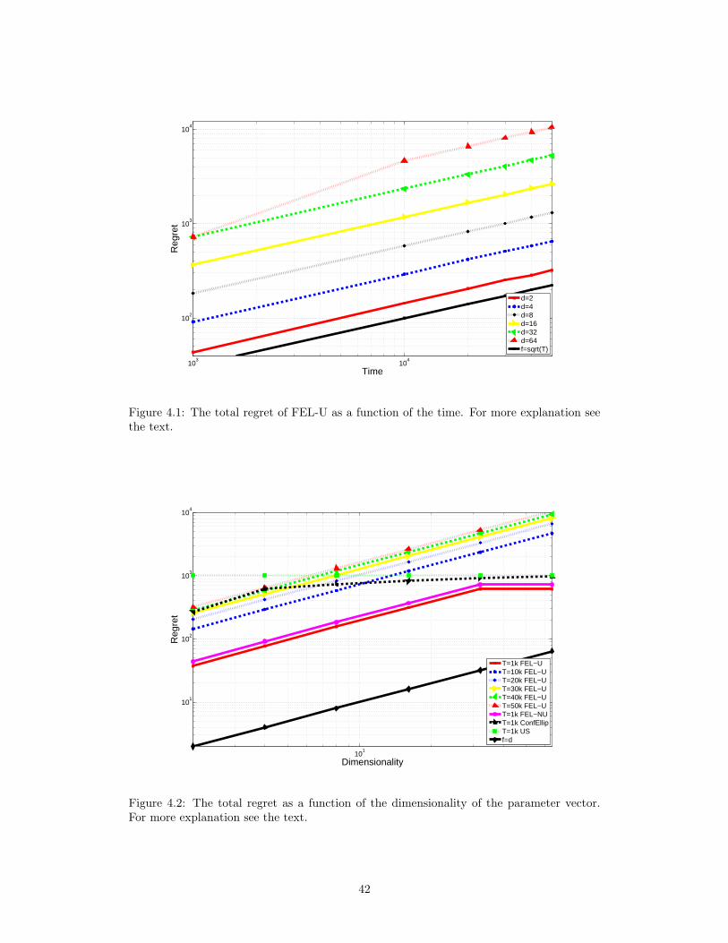
103

104

102

103

104

Time

Reg

ret

d=2d=4d=8d=16d=32d=64f=sqrt(T)

Figure 4.1: The total regret of FEL-U as a function of the time. For more explanation seethe text.

101

101

102

103

104

Dimensionality

Reg

ret

T=1k FEL−UT=10k FEL−UT=20k FEL−UT=30k FEL−UT=40k FEL−UT=50k FEL−UT=1k FEL−NUT=1k ConfEllipT=1k USf=d

Figure 4.2: The total regret as a function of the dimensionality of the parameter vector.For more explanation see the text.

42

We have two interesting observations in Figure 4.2: 1) for T = 1000, the regret of FEL

becomes almost constant for big values of d. Generally, for this class of problems it holds

that (not shown here) if t is fixed and d → ∞, then the regret becomes ct with some

c > 0 that depends on the problem class. 2) The regret of Confidence Ellipsoid Algorithm

is almost constant with respect to d. Actually Confidence Ellipsoid is still in its transient

mode and its regret is ct. The regret of the uniform sampling, referred to as US , is also

included in Figure 4.2. We observe that the regret of ConfEllip is converging to the regret

of US as d → ∞. Based on our observations (again not shown here), it takes a very long

time for Confidence Ellipsoid to exit from its transient mode in this problem (something in

the order of T = 500, 000).

4.2 The Ad Allocation Problem

In the ad allocation problem, a website is provided with a number of ads. At each time

step, the website chooses an ad to display. The website gets paid by each user-click. The

objective is to maximize the number of user-clicks.

Since the number of ads is usually very large, we can not directly apply a K-armed bandit

algorithm such as the popular UCB1 of Auer et al. (2002) to this problem. Fortunately, there

are correlations between the ads and we exploit this property to achieve better performance.

The problem setting, borrowed from Pandey et al. (2007) is as follows: We have C

clusters indexed by i ∈ 1, . . . , C. Let us denote the optimal cluster (cluster containing

the optimal action) by iopt (we refer to ads as actions). Each suboptimal cluster contains

N actions. The optimal cluster contains Nopt actions. The outcome of an action is 0 or 1

and is distributed according to a Bernoulli distribution. Let µopt be the expected payoff of

the optimal action in the optimal cluster, µs be the payoff of the best action among other

clusters, µi be the payoff of the best action in cluster i, and µi,j be the payoff of the jth

action of cluster i. Define ∆ = µopt − µs as the cluster separation. The cohesiveness of

cluster i is defined as follows:

δi =1N

N∑j=1

(µi − µi,j).

Further we let δopt denote the cohesiveness of the optimal cluster.

Following Pandey et al. (2007), we use C = 10 and N = 10 (i.e., the total number of

actions is 100). The configuration is shown in Figure 4.3. For the suboptimal clusters, we

use µi = 0.5 and δi = 0.1. The default values of the parameters of the optimal cluster are

Nopt = 10, δopt = 0.3, and µopt = 0.63. The time horizon is 12000 and we repeat each

experiment 200 times.

Pandey et al. (2007) simply put ads in clusters and use a two-stage UCB1 algorithm. In

the first stage, they choose the cluster and in the second stage, they choose the ad. itself.

43

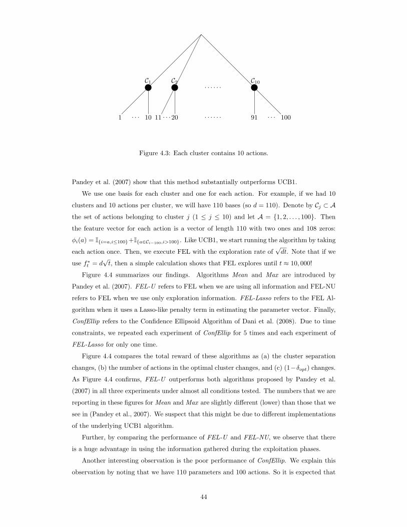
yC1

1 . . . 10

yC2

11 . . .20

@@@@@@@@yC10

91

@@@@

. . . 100

. . . . . .

. . . . . .

Figure 4.3: Each cluster contains 10 actions.

Pandey et al. (2007) show that this method substantially outperforms UCB1.

We use one basis for each cluster and one for each action. For example, if we had 10

clusters and 10 actions per cluster, we will have 110 bases (so d = 110). Denote by Cj ⊂ A

the set of actions belonging to cluster j (1 ≤ j ≤ 10) and let A = 1, 2, . . . , 100. Then

the feature vector for each action is a vector of length 110 with two ones and 108 zeros:

φi(a) = Ii=a,i≤100+Ia∈Ci−100,i>100. Like UCB1, we start running the algorithm by taking

each action once. Then, we execute FEL with the exploration rate of√dt. Note that if we

use f∗t = d√t, then a simple calculation shows that FEL explores until t ≈ 10, 000!

Figure 4.4 summarizes our findings. Algorithms Mean and Max are introduced by

Pandey et al. (2007). FEL-U refers to FEL when we are using all information and FEL-NU

refers to FEL when we use only exploration information. FEL-Lasso refers to the FEL Al-

gorithm when it uses a Lasso-like penalty term in estimating the parameter vector. Finally,

ConfEllip refers to the Confidence Ellipsoid Algorithm of Dani et al. (2008). Due to time

constraints, we repeated each experiment of ConfEllip for 5 times and each experiment of

FEL-Lasso for only one time.

Figure 4.4 compares the total reward of these algorithms as (a) the cluster separation

changes, (b) the number of actions in the optimal cluster changes, and (c) (1−δopt) changes.

As Figure 4.4 confirms, FEL-U outperforms both algorithms proposed by Pandey et al.

(2007) in all three experiments under almost all conditions tested. The numbers that we are

reporting in these figures for Mean and Max are slightly different (lower) than those that we

see in (Pandey et al., 2007). We suspect that this might be due to different implementations

of the underlying UCB1 algorithm.

Further, by comparing the performance of FEL-U and FEL-NU, we observe that there

is a huge advantage in using the information gathered during the exploitation phases.

Another interesting observation is the poor performance of ConfEllip. We explain this

observation by noting that we have 110 parameters and 100 actions. So it is expected that

44

ConfEllip can’t outperform simple UCB1 in this problem. The numbers that Pandey et al.

(2007) report for UCB1 are higher that our results for ConfEllip. Having said that, one

strength of the FEL Algorithm comes from the implicit regularization that is happening

because Ct is initialized with I.

Finally, we observe that FEL-Lasso outperforms all alternative algorithms. We attribute

this performance to the fact that in this problem, the parameter vector is sparse: We expect

10+(a small number) of the elements of the parameter vector be around 1 and the rest of

them be almost 0. This situation is particularly suitable for a method like Lasso.

4.3 FEL vs. UCT

Assume that we have a large action set and no prior information about the correlations

between actions is given. The dominant algorithm for such problems is UCT of Kocsis and

Szepesvari (2006).

UCT is implemented in the following way: Let m be the number of actions. We build

a tree of height logm (so it has m leaves) and put each action on a leaf. We index nodes

by ni where 1 ≤ i ≤ 2m − 1 (for example, we have n2 and n3 at depth 2). For node ni,

we construct a UCB1 algorithm with action set n2i−1, n2i. Further, we use Cp =√

log TTi

instead of√

2 log TTi

as the bonus term. In each timestep, we start from the root and decide

which child to choose according to the UCB1 Algorithm of that node. This process continues

until we reach a leaf where we observe a reward. Now, we update the UCB1 Algorithms of

all parents of this leaf (up to the root) assuming that we have observed this reward when

choosing them.

One might wonder how FEL performs when we have a large uncorrelated action set. In

this section, we compare the performance of FEL with UCT on a toy problem.

The toy problem is constructed as follows: We have 16 actions with payoffs generated uni-

formly randomly: 0.3612, 0.5936, 0.4552, 0.4263, 0.7276, 0.4632, 0.5171, 0.4739, 0.1034,

0.9755, 0.9249, 0.0290, 0.0166, 0.9703, 0.9594, 0.9076. Then we build a tree as described

above and put these actions on the leaves. The basis functions of FEL are built in the fol-

lowing way: Assign a basis function to each node of the tree. This basis is 1 when taking any

action below it. Otherwise, it is 0. So we will have totally 31 basis functions. We use FEL

with f∗t = 10 log t. We also run UCT with Cp =√

2 and with Cp = 0.21√

2. The second

bonus term is tuned such that it gives the best performance for UCT on this problem. The

time horizon is 10,000 and we repeat each experiment 10 times.

Figure 4.5 summarizes our findings and shows that FEL is not really competitive with

UCT. In this figure, UCT-UM (UCT-UnModified) refers to the version of UCT with Cp =

45

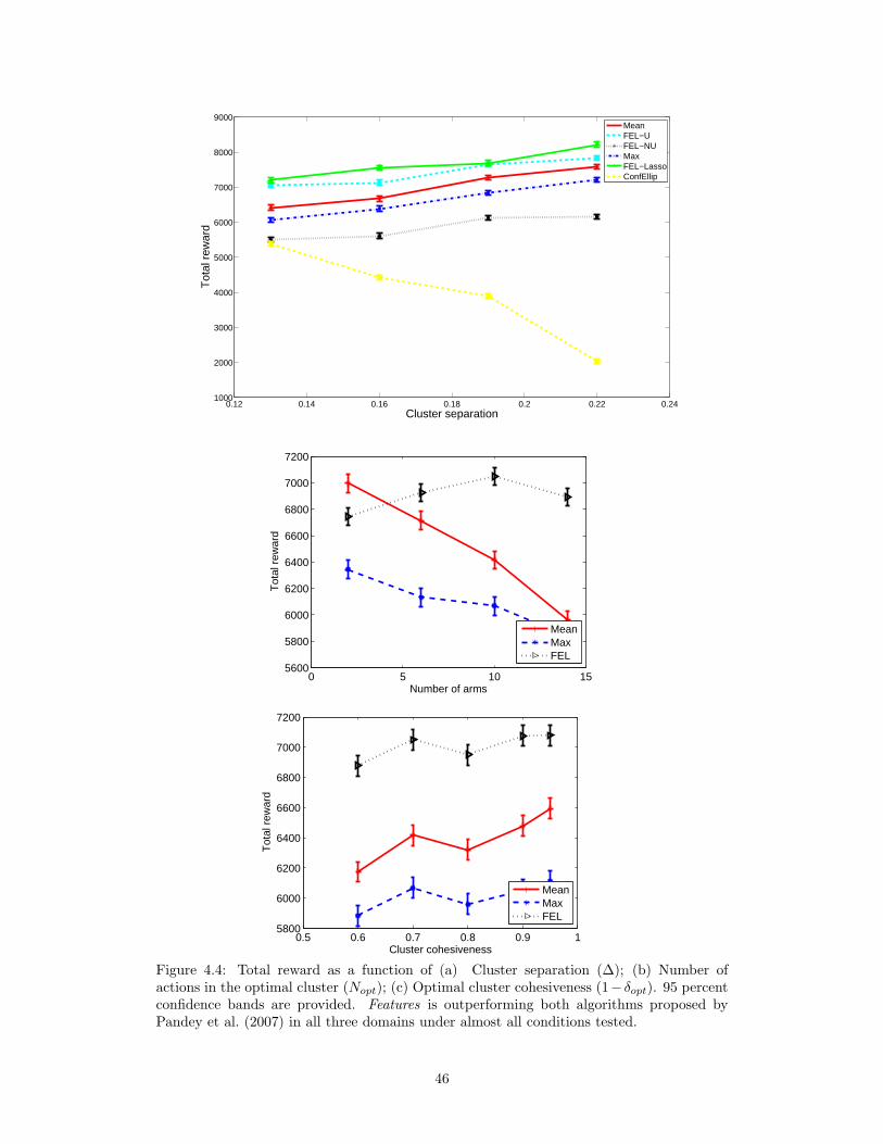
0.12 0.14 0.16 0.18 0.2 0.22 0.241000

2000

3000

4000

5000

6000

7000

8000

9000

Cluster separation

Tot

al r

ewar

d

MeanFEL−UFEL−NUMaxFEL−LassoConfEllip

0 5 10 155600

5800

6000

6200

6400

6600

6800

7000

7200

Number of arms

Tot

al r

ewar

d

MeanMaxFEL

0.5 0.6 0.7 0.8 0.9 15800

6000

6200

6400

6600

6800

7000

7200

Cluster cohesiveness

Tot

al r

ewar

d

MeanMaxFEL

Figure 4.4: Total reward as a function of (a) Cluster separation (∆); (b) Number ofactions in the optimal cluster (Nopt); (c) Optimal cluster cohesiveness (1− δopt). 95 percentconfidence bands are provided. Features is outperforming both algorithms proposed byPandey et al. (2007) in all three domains under almost all conditions tested.

46

0 5000 100000

50

100

150

200

250

Time

Tot

al r

egre

t

UCT−MUCTFEL

Figure 4.5: The regret of FEL compared to the regret of UCT.

√2 and UCT refers to the version of UCT with Cp =

√2.

47

Chapter 5

Conclusions

We studied the linear and continuum-armed bandit problems and explored the idea of how

far the Forced Exploration methods (FEL and FEC) can take us. We analyzed FEL and

found that its regret is bounded by O(d√T ). We provided a simple example to show that this

is the best that least squares method can do in the linear bandit problem (Remark 20). We

also discovered the fact that r(θ) is approximately quadratic in the error in the neighborhood

of θ∗ for a few interesting action spaces. We conclude that FEL can be proven to be

competitive, which is confirmed by the experiments. The experiments also confirm our

conjecture of how the regret of FEL scales with d and T in a number of cases (Section 4.1).

Our experiments go beyond the studied algorithm in two ways: 1) Learn from all data. This

looks like a good idea, though we were not able to prove that this is indeed a good idea. 2)

Learn with a Lasso-like penalty.

We also experimented with the Confidence Ellipsoid Algorithm and found that in one

particular case the Confidence Ellipsoid Algorithm is not competitive with FEL. In this

case, FEL+Lasso is even better than FEL. We provided a heuristic explanation for this

observation.

We applied the techniques to a non-parametric situation and achieved a regret bounded

by O(T

2+α2+2α

), which is known to be a suboptimal rate.

However, the Forced Exploration method has the nice property that one can bound the

expected instantaneous regret for t big enough. This is usually impossible to do for the

bandit algorithms. Further, its implementation is efficient, compared to algorithms like

Confidence Ellipsoid that require solving intractable optimization problems.

Finally, note that all the bounds in this thesis contain problem-dependent constants.

Although it is possible to tune the algorithm so that the performance then can be bounded

in a problem-independent way (assuming a reasonable class e.g. when the expected payoffs

are bounded), the resulting bound scales worse than√T with time. This is not a weakness of

the analysis, but a property of the algorithms considered. Hence the quest for a practically

good performing, computationally efficient algorithm with provable uniform O(√T ) regret

48

bound and which scales with dimension in an optimal manner is still open.

Bibliography

A. Antos, V. Grover, and C. Szepesvari. Active learning in multi-armed bandits. In

ALT-2008, pages 287–302, 2008.

J.-Y. Audibert, R. Munos, and Cs. Szepesvari. Exploration-exploitation trade-off using

variance estimates in multi-armed bandits. In Theoretical Computer Science-2008, 2008.

P. Auer. Using confidence bounds for exploitation-exploration trade-offs. Journal of Machine

Learning Research, 3:397–422, 2002.

P. Auer. Personal communication, 2007.

P. Auer, N. Cesa-Bianchi, and P. Fischer. Finite time analysis of the multiarmed bandit

problem. Machine Learning, 47(2-3):235–256, 2002.

P. Auer, R. Ortner, and Cs. Szepesvari. Improved rates for the stochastic continuum-armed

bandit problem. In Proceedings of the 20th Annual Conference on Learning Theory

(COLT-07), pages 454–468, 2007.

N. Cesa-Bianchi and G. Lugosi. Prediction, Learning, and Games. Cambridge University

Press, New York, NY, USA, 2006.

E. Cope. Regret and convergence bounds for a class of continuum-armed bandit problems.

(submitted), 2006.

V. Dani, T.P. Hayes, and S.M. Kakade. Stochastic linear optimization under bandit feed-

back. COLT-2008, pages 355–366, 2008.

M. French, C. Szepesvari, and E. Rogers. Performance of Nonlinear Approximate Adaptive

Controllers. Wiley, 2003.

R.C. Gunning and H. Rossi. Analytic Functions of Several Complex Variables. Prentice-Hall,

New York, 1965.

W. Hoeffding. Probability inequalities for sums of bounded random variables. Journal of

the American Statistical Association, 58:13–30, 1963.

W. Karush. Minima of functions of several variables with inequalities as side constraints.

Master’s thesis, Department of Mathematics, University of Chicago, 1939.

R.D. Kleinberg. Nearly tight bounds for the continuum-armed bandit problem. In

NIPS-2004, 2004.

49

R.D. Kleinberg. Online Decision Problems with Large Strategy Sets. PhD thesis, Depart-

ment of Mathematics, Massachusetts Institute of Technology, 2005.

L. Kocsis and Cs. Szepesvari. Bandit based monte-carlo planning. In ECML-2006, pages

282–293, 2006.

T. L. Lai and H. Robbins. Asymptotically efficient adaptive allocation rules. Advances in

Applied Mathematics, 6:4–22, 1985.

V.B. Melas. Functional Approach to Optimal Experimental Design. Springer, 2006.

J. Nocedal and S.J. Wright. Numerical Optimization. Springer, 2006.

S. Pandey, D. Chakrabarti, and D. Agarwal. Multi-armed bandit problems with dependent

arms. In ICML-2007, pages 721–728, 2007.

H. Robbins. Some aspects of the sequential design of experiments. Bulletin of the American

Mathematical Society, 58:527–535, 1952.

J. Shawe-Taylor and N. Cristianini. Kernel Methods for Pattern Analysis. Cambridge

University Press, 2004.

G.W. Stewart and Ji-guang Sun. Matrix Perturbation Theory. Academic Press, 1990.

W.R. Thompson. On the likelihood that one unknown probability exceeds another in view

of the evidence of two samples. Biometrika, 25:285–294, 1933.

50

Appendix A

Background in Calculus

Definition 3 (Point-wise Holder function). Let A ∈ Rd, h : A → R, a∗ ∈ A. If ∃L, β > 0

such that for all a ∈ A, h(a∗)− h(a) ≤ L|a∗ − a|β then we say that function h is Holder at

a∗ with constant L and exponent β.

Definition 4 (Uniformly locally Holder function). Let A ∈ Rd, h : A → R, a∗ ∈ A. If

∃δ, L, β > 0 such that for all a, a′ ∈ A with ‖a− a′‖ ≤ δ,

‖h∗(a)− h∗(a′)‖ ≤ L‖a− a′‖β

then we say that function h is Holder with constant L, exponent β, and neighborhood δ.

The next theorem is stated in the form given here as Theorem 1.8.1 in Melas (2006).

The original version can be found in Gunning and Rossi (1965), Chapter 1.

Theorem 31 (Implicit Function Theorem). Let G : Rs+k 7→ Rs be a function and fix

u0 ∈ Rk such that

• the equation G(v, u0) = 0 has a solution v0; and

• the function G is continuous and has continuous first partial derivatives ∂∂ui

G(v, u),∂∂vj

G(v, u), for 1 ≤ i ≤ k and 1 ≤ j ≤ s in the neighborhood of (u0, v0) and

• det[∂∂vj

Gi(v0, u0)]si,j=1

6= 0.

Then there exists a neighborhood U of the point u0 and function g : U → Rs such that in U

we have (1) G(u, g(u)) = 0, (2) v0 = g(u0), (3) g is continuous and

J(g(u), u)∂g(u)∂uj

= −Lj(g(u), u), j = 1, . . . , k,

where

J(v, u) =[∂

∂vjGi(v, u)

]si,j=1

, Lj(v, u) =[∂

∂ujGi(v, u)

]si=1

.

Further, if g : U → Rs satisfies (1) and (2) then g = g.

51

The following theorem can be found in Karush (1939):

Theorem 32 (Karush-Kuhn-Tucker Theorem). Consider the following optimization prob-

lem:

f(x)→ min! s.t.

g(x) ≤ 0,

h(x) = 0,

where f : Rn → R, g : Rn → R and h : Rn → R are continuously differentiable functions at

x∗. Assume that x∗ is a local minimum and ∇g(x) and ∇h(x) are linearly independent at

x∗. Then there exists constants µ and λ such that the following holds:

∇f(x∗) + µ∇g(x∗) + λ∇h(x∗) = 0,

g(x∗) ≤ 0, h(x∗) = 0,

µ ≥ 0,

µg(x∗) = 0.

The following definition is stated by French et al. (2003):

Definition 5 (Sobolev spaces). Let 1 ≤ p ≤ +∞ and α ≥ 1 be integers. Let A ⊂ Rd

be an open connected domain. Define Wα(Lp(A)) as the set of all measurable functions h

defined on A whose distributional derivatives Dωh, |ω| ≤ α, lie in Lp(A). Here Dω is the

distributional derivative of h with respect to the multi-index ω = (ω1, . . . , ωd), which means

(Dωh)(x) =

(∂(ω1)

∂a(ω1)1

. . .∂(ωd)

∂a(ωd)d

h

)(a),

and

|ω| = |ω1|+ · · ·+ |ωd| .

The semi-norm for Wα(Lp(A)) is defined by

|h|Wα(Lp(A)) = ∑

|ω|=α ‖Dαh‖Lp(A) , if 1 ≤ p ≤ ∞,max|ω|=α ‖Dαh‖L∞(A) , otherwise,

and the norm by

‖h‖Wα(Lp(A)) = |h|Wα(Lp(A)) + ‖h‖Lp(A) .

The next proposition is stated in the form given here as Lemma 7 in Antos et al. (2008).

Proposition 33. Let q(t) = at+ b, l(t) = log t, where a > 0. Then for any t ≥ (2/a)(−b+

log(1/a)), q(t) ≥ l(t).

52

Appendix B

Exponential Tail Inequalities

We use the following bounds throughout this thesis:

Theorem 34 (Hoeffding’s inequality (Hoeffding, 1963)). If X1, . . . , Xn are independent and

ai ≤ Xi ≤ bi(i = 1, 2, . . . , n), then for t > 0

P(X − µ ≥ t

)≤ exp

(−2n2t2∑n

i=1(bi − ai)2

)where X =

∑ni=1Xi/n and µ = E

[X].

The next theorem stated as Lemma A.7 in (Cesa-Bianchi and Lugosi, 2006) is the ex-

tension of Hoeffding’s inequality to the martingales:

Theorem 35 (Hoeffding-Azuma inequality). Let V1, V2, . . . be a martingale difference se-

quence with respect to some sequence X1, X2, . . . such that Vi ∈ [Ai, Ai + ci] for some

random variable Ai, measurable with respect to X1, . . . , Xi−1 and a positive constant ci. If

Sn =∑ni=1 Vi, then for any t > 0,

P (Sn > t) ≤ exp(−2t2∑ni=1 c

2i

)and

P (Sn < −t) ≤ exp(−2t2∑ni=1 c

2i

)Next, we have Bernstein’s inequality :

Theorem 36 (Bernstein’s inequality). Let (Xt,Ft) be a bounded martingale difference series

with |Xt| ≤ R w.p.1. Then, for any n ≥ 1, V > 0, 0 < δ < 1, the simultaneous inequalities

n∑t=1

Xt ≥√

2V x+2Rx

3,

n∑t=1

E[X2t |Ft−1

]≤ V

hold with probability at most δ, where x = log(1/δ).

Finally, we have McDiarmid’s inequality (Shawe-Taylor and Cristianini, 2004):

53

Theorem 37 (McDiarmid’s inequality). Let X1, . . . , Xn be independent random variables

taking values in a set X , and assume f : Xn → R satisfies

supx1,...,xn,xi∈A

|f(x1, . . . , xn)− f(x1, . . . , xi−1, xi, xi+1, . . . , xn)| ≤ ci, 1 ≤ i ≤ n.

Then for all ε > 0,

P (f(X1, . . . , Xn)− E [f(X1, . . . , Xn)] ≥ ε) ≤ exp(−2ε2∑ni=1 c

2i

).

54