Library 1666: Electrical Engineering - bplacedsoftware49g.bplaced.net/EnglishSeite01/ElectricalEngineeringFor... · 7 4. Using the library Electrical Engineering is a fast and easy

1

Library 1666: Electrical Engineering Table Of Contents: 1. Disclaimer & Copyright ...............................................................................5 2. Credits ........................................................................................................5 3. System Requirements & Installation...........................................................6 3.1. System Requirements ................................................................................6 3.2. Installation & Deinstallation.........................................................................6 4. Using the library..........................................................................................7 4.1. Overview.....................................................................................................8 4.2. Starting Electrical Engineering..................................................................12 5. Introduction to Analysis.............................................................................13 6. Introduction to Equations..........................................................................14 6.1. Choosing a set of equations of a subtopic................................................14 6.2. Choosing all equations of a subtopic ........................................................15 6.3. Choosing a single equation of a subtopic .................................................15 7. Using Analysis ..........................................................................................16 7.1. AC Circuits................................................................................................16 7.1.1. Impedance Calculations ...........................................................................16 7.1.2. Voltage Divider .........................................................................................17 7.1.3. Current Divider .........................................................................................18 7.1.4. Circuit Performance..................................................................................19 7.1.5. AC Circuits Command Line Programs......................................................20 7.2. Polyphase Circuits....................................................................................21 7.2.1. Wye �

� Conversion................................................................................21

7.2.2. Balanced Wye Load..................................................................................22 7.2.3. Balanced

� Load ......................................................................................22

7.2.4. Polyphase Circuits Command Line Programs ..........................................23 7.3. Ladder Network ........................................................................................24 7.4. Filter Design .............................................................................................27 7.4.1. Chebyshev Filter.......................................................................................27 7.4.2. Butterworth Filter ......................................................................................28 7.4.3. Active Filter...............................................................................................29 7.4.4. Filter Design Command Line Programs....................................................30 7.5. Gain and Frequency .................................................................................31 7.5.1. Transfer Function .....................................................................................31 7.5.2. Bode Plots ................................................................................................32 7.5.3. Gain and Frequency Command Line Programs .......................................33 7.6. Fourier Transforms ...................................................................................34 7.6.1. FFT...........................................................................................................34 7.6.2. Inverse FFT ..............................................................................................34 7.6.3. Fourier Transforms Command Line Programs .........................................35 7.7. Two-Port Networks ...................................................................................36 7.7.1. Parameter Conversion..............................................................................36 7.7.2. Circuit Performance..................................................................................37 7.7.3. Interconnected Two-Ports.........................................................................38 7.7.4. Two-Port Networks Command Line Programs .........................................39 7.8. Transformer Performance.........................................................................40 7.8.5. Open Circuit Test......................................................................................40

2

7.8.6. Short Circuit Test......................................................................................41 7.8.7. Chain Parameters.....................................................................................41 7.8.8. Transformer Performance Command Line Programs...............................42 7.9. Transmission Lines...................................................................................43 7.9.9. Open Circuit Test......................................................................................43 7.9.10. Line Parameters .......................................................................................44 7.9.11. Fault Location Estimate ............................................................................44 7.9.12. Lossless Line Impedance .........................................................................45 7.9.13. Transmission Lines Command Line Programs .........................................45 7.10. Error Functions .........................................................................................46 7.10.1. Using Error Functions...............................................................................46 7.10.2. Error Functions Command Line Programs ...............................................46 8. Using Equations .......................................................................................47 8.1. Resistive Circuits ......................................................................................47 8.1.1. Resistance and Conductance...................................................................47 8.1.2. Ohm’s Law and Power..............................................................................49 8.1.3. Temperature Effect...................................................................................50 8.1.4. Maximum DC Power Transfer ..................................................................51 8.1.5. V and I Source Equivalence .....................................................................52 8.2. Capacitance and Electric Fields ...............................................................53 8.2.6. Point Charge.............................................................................................53 8.2.7. Long Charged Line ...................................................................................54 8.2.8. Charged Disk............................................................................................55 8.2.9. Parallel Plates...........................................................................................56 8.2.10. Parallel Wires ...........................................................................................57 8.2.11. Coaxial Cable ...........................................................................................58 8.2.12. Sphere......................................................................................................59 8.3. Inductors and Magnetism .........................................................................60 8.3.1. Long Line..................................................................................................60 8.3.2. Long Strip .................................................................................................61 8.3.3. Parallel Wires ...........................................................................................62 8.3.4. Loop..........................................................................................................63 8.3.5. Coaxial Cable ...........................................................................................64 8.3.6. Skin Effect ................................................................................................65 8.4. Inductors and Magnetism .........................................................................66 8.4.1. Electron Beam Deflection .........................................................................66 8.4.2. Thermionic Emission ................................................................................68 8.4.3. Photoemission ..........................................................................................69 8.5. Meters and Bridge Circuits .......................................................................70 8.5.1. Amp, Volt, Ohmmeter ...............................................................................70 8.5.2. Wheatstone Bridge ...................................................................................71 8.5.3. Wien Bridge ..............................................................................................72 8.5.4. Maxwell Bridge .........................................................................................73 8.5.5. Owen Bridge.............................................................................................74 8.5.6. Symmetrical Resistive Attenuator.............................................................75 8.5.7. Unsymmetrical Resistive Attenuator.........................................................76 8.6. RL and RC Circuits...................................................................................77 8.6.1. RL Natural Response ...............................................................................77 8.6.2. RC Natural Response...............................................................................79 8.6.3. RL Step Response ...................................................................................80 8.6.4. RC Step Response...................................................................................81 8.6.5. RL Series to Parallel .................................................................................82

3

8.6.6. RC Series to Parallel ................................................................................83 8.7. RLC Circuits .............................................................................................84 8.7.1. Series Impedance.....................................................................................84 8.7.2. Parallel Admittance...................................................................................85 8.7.3. RLC Natural Response.............................................................................86 8.7.4. Underdamped Transient ...........................................................................87 8.7.5. Critical-Damped Transient ........................................................................88 8.7.6. Overdamped Transient .............................................................................89 8.8. AC Circuits................................................................................................90 8.8.1. RL Series Impedance ...............................................................................90 8.8.2. RC Series Impedance...............................................................................91 8.8.3. Impedance � Admittance ........................................................................92 8.8.4. Two Impedances in Series .......................................................................93 8.8.5. Two Impedances in Parallel......................................................................94 8.9. Polyphase Circuits....................................................................................95 8.9.1. Balanced � Network .................................................................................95 8.9.2. Balanced Wye Network ............................................................................96 8.9.3. Power Measurements...............................................................................97 8.10. Electrical Resonance................................................................................98 8.10.1. Parallel Resonance I.................................................................................98 8.10.2. Parallel Resonance II................................................................................99 8.10.3. Resonance in Lossy Inductor .................................................................100 8.10.4. Series Resonance ..................................................................................101 8.11. OpAmp Circuits ......................................................................................102 8.11.1. Basic Inverter..........................................................................................102 8.11.2. Non-Inverting Amplifier ...........................................................................103 8.11.3. Current Amplifier.....................................................................................104 8.11.4. Transconductance Amplifier ...................................................................105 8.11.5. Level Detector (Inverting) .......................................................................106 8.11.6. Level Detector (Non-Inverting)................................................................107 8.11.7. Differentiator ...........................................................................................108 8.11.8. Differential Amplifier................................................................................109 8.12. Solid State Devices.................................................................................110 8.12.1. Semiconductor Basics ............................................................................110 8.12.2. PN Junctions ..........................................................................................112 8.12.3. PN Junction Currents..............................................................................114 8.12.4. Transistor Currents.................................................................................116 8.12.5. Ebers-Moll Equations..............................................................................117 8.12.6. Ideal Currents - pnp................................................................................118 8.12.7. Switching Transients...............................................................................119 8.12.8. MOS Transistor I ....................................................................................120 8.12.9. MOS Transistor II ...................................................................................121 8.12.10. MOS Inverter (Resistive Load) ...............................................................122 8.12.11. MOS Inverter (Saturated Load) ..............................................................124 8.12.12. MOS Inverter (Depletion Load)...............................................................126 8.12.13. CMOS Transistor Pair.............................................................................127 8.12.14. Junction FET ..........................................................................................128 8.13. Linear Amplifiers.....................................................................................129 8.13.1. BJT (Common Base) ..............................................................................129 8.13.2. BJT (Common Emitter) ...........................................................................131 8.13.3. BJT (Common Collector) ........................................................................132 8.13.4. FET (Common Gate) ..............................................................................133

4

8.13.5. FET (Common Source)...........................................................................134 8.13.6. FET (Common Drain) .............................................................................135 8.13.7. Darlington (CC-CC) ................................................................................136 8.13.8. Darlington (CC-CE).................................................................................137 8.13.9. Emitter-Coupled Amplifier.......................................................................138 8.13.10. Differential Amplifier................................................................................139 8.13.11. Source-Coupled JFET Pair.....................................................................140 8.14. Class A, B and C Amplifiers....................................................................141 8.14.1. Class A Amplifier ....................................................................................141 8.14.2. Power Transistor ....................................................................................143 8.14.3. Push-Pull Principle .................................................................................144 8.14.4. Class B Amplifier ....................................................................................145 8.14.5. Class C Amplifier ....................................................................................146 8.15. Transformers ..........................................................................................147 8.15.1. Ideal Transformer ...................................................................................147 8.15.2. Linear Equivalent Circuit.........................................................................149 8.16. Motors and Generators...........................................................................150 8.16.1. Energy Conversion .................................................................................150 8.16.2. DC Generator .........................................................................................152 8.16.3. Separately-Excited DC Generator ..........................................................153 8.16.4. DC Shunt Generator...............................................................................154 8.16.5. DC Series Generator ..............................................................................155 8.16.6. Separately-Excited DC Motor .................................................................156 8.16.7. DC Shunt Motor......................................................................................157 8.16.8. DC Series Motor .....................................................................................158 8.16.9. Permanent Magnet Motor .......................................................................159 8.16.10. Induction Motor I.....................................................................................160 8.16.11. Induction Motor II....................................................................................161 8.16.12. Single-Phase Induction Motor.................................................................162 8.16.13. Synchronous Machines ..........................................................................163 9. Used Keys ..............................................................................................165 10. Things To Do..........................................................................................167 11. Version History .......................................................................................167 12. Known Bugs ...........................................................................................167

5

1. Disclaimer & Copyright This program is for your private use only and is provided "as is". This software is not sold, only the right for using it is granted. Using this software is only allowed on the calculator the software has been licensed for. This program has been tested but may contain errors. I’m making no warranty of any kind with regard to this software, including, but not limited to, the implied warranties of merchantability and fitness for a particular purpose. I shall not be liable for any errors or for incidental or consequential damages in connection with the furnishing, performance, or use of this software. Suggestions, criticism and/or improvement suggestions can be send to the author at [email protected]. All rights reserved. © Andreas Möller 2013 2. Credits Thanks to ACO for the HP 49G, Wolfgang Rautenberg for OT49, Eduardo M. Kalinowski for “Programming in System RPL”, Mika Heiskanen for BZ and various post from different authors in comp.sys.hp48. Without them this program couldn’t been written.

6

3. System Requirements & Installation 3.1. System Requirements Library 1666: Electrical Engineering has been coded and compiled with Debug4x and is written in System RPL. It is designed for the HP 49G+ and HP 50G. Electrical Engineering requires TreeBrowser and GUISLV/GUIMES. Both must be installed in order to use Electrical Engineering. If you are not familiar about TreeBrowser and GUISLV/GUIMES then please read the documentations that comes with it. 3.2. Installation & Deinstallation Use the installation program EEI on the SD card to install / update / modify / delete the Electrical Engineering library. Insert the SD card into the turned off calculator and then power up the calculator. Now start the installation program EEI from the SD card. -> in RPN mode key in :3:EEI [ENTER] [EVAL] -> in ALG mode key in EVAL(:3:EEI) [ENTER] The installation program will guide you through the installation process.

7

4. Using the library Electrical Engineering is a fast and easy to use software and an invaluable aid in solving a variety of practical problems encountered by both students and professionals in electrical engineering. Designed for speed, accuracy, and ease of use, this software gives the user the ability to find quick solutions to sets of complex problems. Electrical Engineering contains over 500 advanced electrical engineering analysis routines plus over 500 electrical engineering equations (including variable descriptions, units and pictures) whereby covering the undergraduate curriculum for electrical engineers in most universities.

8

4.1. Overview Analysis : • AC Circuits – Impedance calculations – Voltage and Current dividers – Circuit Performance • Polyphase Circuits – Wye � � conversion – Balanced Wye Load – Balanced � Load. • Ladder Network • Filter Design – Chebyshev Filter – Butterworth Filter – Active Filter • Gain and Frequency – Transfer function – Bode Plots • Fourier Transforms – FFT – Inverse FFT • Two-port Networks – Parameter Conversion for z, y, h, g, a, and b parameters – Circuit Performance – Interconnected Two-Ports • Transformer Performance – Open Circuits Test – Short Circuits Test – Chain Parameters • Transmission Lines – Line Characteristics – Line Parameters – Fault Location Estimate – Lossless Line Impedance • Error Functions – Using error and complementary error functions

9

Equations : • Resistive Circuits – Resistance and Conductance – Ohm's Law and Power – Temperature Effect – Maximum Power Transfer – V and I Source Equivalent • Capacitance and Electric Fields – Point Charge – Long Charged Line – Charged Disk – Parallel Plates – Parallel Wires – Coaxial Cable – Sphere • Inductance and Magnetism – Long Line – Long Strip – Parallel Wires – Loop – Coaxial Cable – Skin Effect • Electron Motion – Electron Beam Deflection – Thermionic Emission – Photoemission. • Meters and Bridge Circuits – Amp, Volt, Ohmmeter – Wheatstone Bridge – Wien Bridge – Maxwell Bridge – Owen Bridge – Symmetrical attenuators – Unsymmetrical attenuators • RL and RC Circuits – RL Natural Responses – RC Natural Responses – RL Step Responses – RC Step Responses – RL Series to Parallel – RC Series to Parallel • RLC Circuits – Series Impedance – Parallel Admittance, – RLC Natural Response – Underdamped Transient – Critically-Damped Transient – Overdamped Transient

10

• AC Circuits – RL Series Impedance – RC Series Impedance – Impedance � Admittance – Two Impedances in Series – Two Impedances in Parallel • Polyphase Circuits – Balanced � Network – Balanced Wye Network – Power Measurements • Electrical Resonance – Parallel Resonance I – Parallel Resonance II – Resonance in Lossy Inductor Series Resonance • OpAmp Circuits – Basic Inverter – Non-Inverting Amplifier – current amplifier – Transconductance Amplifier – Level Detector (Inverting) – Level Detector (Non-Inverting) – Differentiator – Differential Amplifier • Solid State Devices – Semiconductor Basics – PN Junctions – PN Junction Currents – Transistor Currents – Ebers-Moll Equations – Ideal Currents - pnp – Switching Transients – MOS transistors I – MOS transistors II – MOS inverter (Resisitve) – MOS inverter (Saturated) – MOS inverter (Depletion) – CMOS Transistor Pair – Junction FET • Linear Amplifiers – BJT (Common Base) – BJT (Common Emitter – BJT (Common Collector) – FET (Common Source) – FET (Common Gate) – FET (Common Drain) – Darlington configuration (CC-CC) – Darlington configuration (CC-CE) – Emitter-coupled Amplifier – Differential Amplifier – Source-coupled JFET Pairs

11

• Class A, B and C Amplifiers – Class A Amplifier – Power Transistors – Push-Pull Principle – Class B Amplifier – Class C amplifiers • Transformers – Ideal Transformers – Linear Equivalent Circuits • Motors & Generators – Energy Conversion – DC Generator – Separately-Excited DC Generator – DC Shunt Generator – DC Series Generator – Separately-Excited DC motor – DC Shunt Motor – DC Series Motor – Permanent Magnet Motor – Induction Motor I – Induction Motor II – Single-Phase Induction Motor – Synchronous Machines

12

4.2. Starting Electrical Engineering Electrical Engineering can be started in different ways. Through the G key

or through the library menu via @á.

13

5. Introduction to Analysis The analysis section of the software is able to perform calculations for a wide range of topics in circuit and electrical network design. A variety of input and output formats are encountered in the different topics of analysis. Analysis routines have been organized into sections, each containing tools for performing electrical analysis of a variety of circuit types. One can design filters, solve two-port networks problems, calculate transmission line properties, minimize logic networks, draw Bode diagrams, etc. - all with context sensitive assistance displayed in the help line. Results can be pushed to the stack for further usage or can be taken from there as an input for the current field (through the M key). Note that units can not be used with complex numbers in the HP 49g series. If you are using complex numbers, than the unit handling must be done by you. The analysis routines are indispensable tools for performing quick calculations. Analysis screens display a list of fields for entering and displaying data. The main part input screen contains input fields for data entry comparisons and result for displaying computed results. The help text at the bottom of the screen describes the action required for the highlighted field or type of result displayed. If the cursor is in an input field then ƒ: toggles title W: allows switching font height X: toggles help line

14

6. Introduction to Equations In the equations section of the software one can select several equation sets from a particular sub-topic, display all the variables used in the set of equations, enter the values for the known variables and solve for the unknown variables. The equations in each subtopic can be solved individually, collectively or as a subset. A unit management feature allows easy entry and display of results. 6.1. Choosing a set of equations of a subtopic Move the cursor to a subtopic and then press I to open a choose box to select the equations which will be passed to the Multiple Equation Solver.

15

6.2. Choosing all equations of a subtopic Move the cursor to a subtopic and then press G to start the Multiple Equation Solver with all equations of that subtopic.

6.3. Choosing a single equation of a subtopic Move the cursor to the equation of a subtopic and then press G

16

7. Using Analysis

7.1. AC Circuits

7.1.1. Impedance Calculations Example: Compute the impedance of a series RLC circuit consisting of a 10_Ohm resistor, a 1.5_Henry inductor and a 4.7_Farad capacitor at a frequency of 100_Hertz. Solution:

17

7.1.2. Voltage Divider Example: Calculate the voltage drop across a series of loads connected to a voltage source of (110+15*i) volts. The load consists of a 50 ohm resistor and impedances of (75+22*i) and (125-40*i) ohms. Solution:

18

7.1.3. Current Divider Example: Calculate the voltage drop across impedances connected in parallel to a current source of (50+25*i). The load consists of a 50 ohm resistor and impedances of (75+22*i) and (125-40*i) ohms. Solution:

19

7.1.4. Circuit Performance Example: Calculate the performance parameters of a circuit consisting of a current source (10-5*i) with a source admittance of (0.0025-0.0012*i) and a load of (0.0012+0.0034*i). Solution:

20

7.1.5. AC Circuits Command Line Programs

VZDIV: Voltage Divider Load Type Impedance VYDIV: Voltage Divider Load Type Admittance CZDIV: Current Divider Load Type Impedance CYDIV: Current Divider Load Type Admittance ZCPERF: Circuit Performance Load Type Impedance YCPERF: Circuit Performance Load Type Admittance

21

7.2. Polyphase Circuits

7.2.1. Wye �

� Conversion

Example: Compute the Wye impedance equivalent of a

� network with impedances (75+12*i),

(75-12*i), and 125 ohms. Solution:

22

7.2.2. Balanced Wye Load Example: A Wye network consists of three impedances of (50+25*i) with a line voltage of 110 volts across line 1 and 2. Find the line current and power measured in a two-wattmeter measurement system. Solution:

7.2.3. Balanced

� Load

Example: A Delta network consists of three impedances of (50-25*i) with a line voltage of 110 volts across line A and B. Find the line current and power measured in a two-wattmeter measurement system. Solution:

23

7.2.4. Polyphase Circuits Command Line Programs

Y��: Wye �

� Conversion Input Type Y�� Y: Wye � �

Conversion Input Type ��Y �

LOAD: Balanced �

Load YLOAD: Balanced Wye Load

24

7.3. Ladder Network

Example : A transistor amplifier is characterized by a base resistance of 2500_

�, a current gain

of 100_A and is operating at a frequency of 10000_Hertz.

This schematic can be reduced to a ladder network consisting of a parallel capacitor of 318_pF and a controlled current of 2500_

� for rb and 100_A for �, a parallel

resistor of 1_M�

and a series capacitor of 0.638_µF.

25

Solution:

26

27

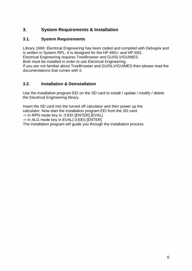
7.4. Filter Design

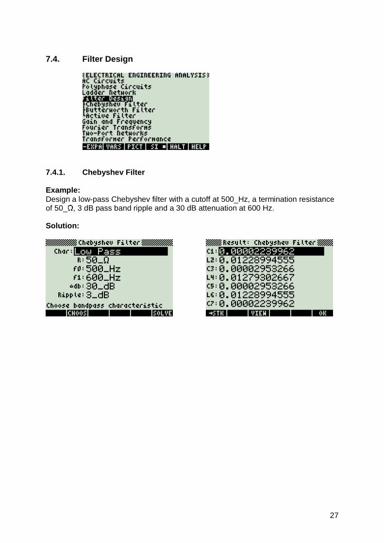
7.4.1. Chebyshev Filter Example: Design a low-pass Chebyshev filter with a cutoff at 500_Hz, a termination resistance of 50_

�, 3 dB pass band ripple and a 30 dB attenuation at 600 Hz.

Solution:

28

7.4.2. Butterworth Filter Example: Design a 100_Hz wide Butterworth band pass filter centered at 800_Hz with a 30_dB attenuation at 900_Hz. The termination and source resistance is 50_

�.

29

7.4.3. Active Filter Example: Design a High Pass active filter with a cutoff at 10_Hz, a midband gain of 10_dB, a quality factor of 1 and a capacitor of 1_µF.

30

7.4.4. Filter Design Command Line Programs

CHLP: Chebyshev Filter Low Pass CHHP: Chebyshev Filter High Pass CHBP: Chebyshev Filter Band Pass CHBE: Chebyshev Filter Band Elimination

BWLP: Butterworth Filter Low Pass BWHP: Butterworth Filter High Pass BWBP: Butterworth Filter Band Pass BWBE: Butterworth Filter Band Elimination

ACLP: Active Filter Low Pass ACHP: Active Filter High Pass ACBP: Active Filter Band Pass

31

7.5. Gain and Frequency

7.5.1. Transfer Function Example: Find the transfer function and its partial fraction expansion for a circuit with a zero located at -10_r/s and three poles located at -100_r/s, -1000_r/s and -5000_r/s. Assume that the multiplier constant is 100000. Solution:

The function is stored automatically as 'Hs' in the current directory. Bode Plots will automatically use this function, if it is present.

32

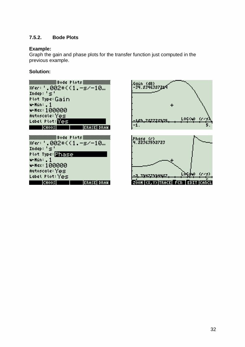
7.5.2. Bode Plots Example: Graph the gain and phase plots for the transfer function just computed in the previous example. Solution:

33

7.5.3. Gain and Frequency Command Line Programs

XFERPZ: Transfer Function Roots XFERND: Transfer Function Coefficients PFER: Partial Fraction Expansion Roots PFEC: Partial Fraction Expansion Coefficients

34

7.6. Fourier Transforms

7.6.1. FFT Example: Find spectral coefficients for the periodic time signal [1 2 3 4]. Solution:

7.6.2. Inverse FFT Example: Find spectral coefficients for the periodic time signal [1 2 3 2 1]. Solution:

35

7.6.3. Fourier Transforms Command Line Programs

�FFT: Fast Fourier Transformation FFT�: Inverse Fast Fourier Transformation

36

7.7. Two-Port Networks

7.7.1. Parameter Conversion Example: Convert a resistive two-port network with z11 = 10_

�, z12 = 7.5_

�, z21 = 7.5_

�,

z22 = 9.375_�

into its equivalent h values. Solution:

37

7.7.2. Circuit Performance Example: A transistor has the following h-parameters: h11 = 10_

�, h12 = 1.2_

� h21= -200_

�,

h22= .000035_�

. The source driving this transistor is a 2_V source with a source impedance of 25_

�. The output port is connected to a 50_

� load. Find the

performance characteristics of the circuit. Solution:

38

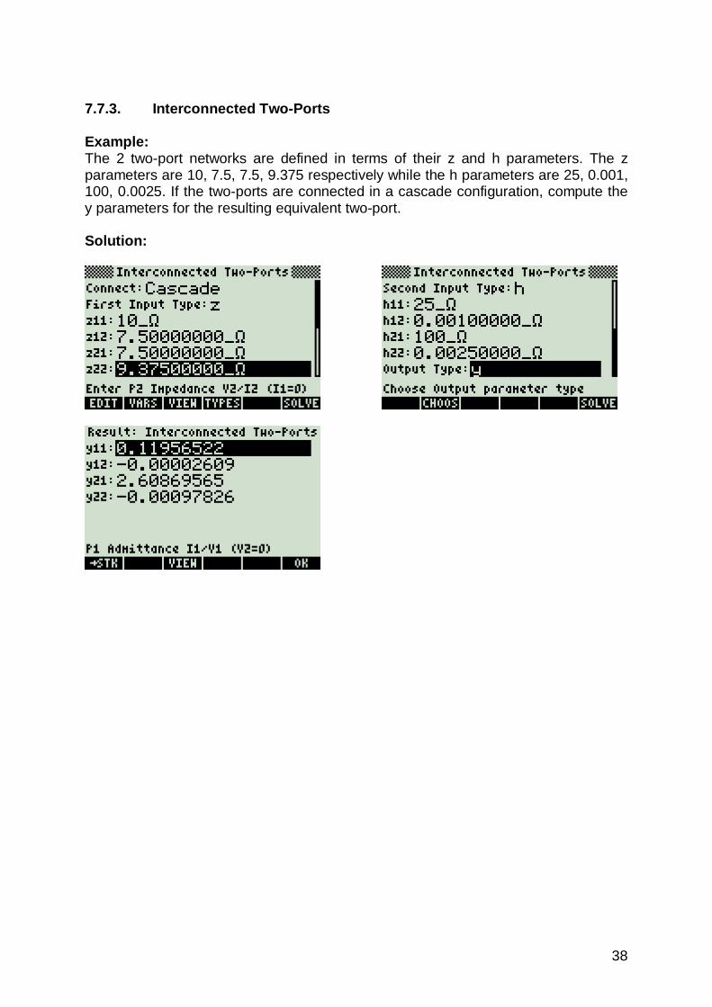
7.7.3. Interconnected Two-Ports Example: The 2 two-port networks are defined in terms of their z and h parameters. The z parameters are 10, 7.5, 7.5, 9.375 respectively while the h parameters are 25, 0.001, 100, 0.0025. If the two-ports are connected in a cascade configuration, compute the y parameters for the resulting equivalent two-port. Solution:

39

7.7.4. Two-Port Networks Command Line Programs

PCONV: Two-Port Networks Parameter Conversion "Input_Type" %Real_11 %Real_12 %Real_21 %Real_22 "Output_Type" � OutTyp_%Real_11 OutTyp_%Real_12 OutTyp_%Real_21 OutTyp_%Real_22 PCPERF: Two-Port Networks Circuit Performance "Input_Type" %Real_11 %Real_12 %Real_21 %Real_22 %Real_Vs %Real_Zs %Real_ZL � Zin Iout Vout Zout I2/I1 V2/V1 V2/Vs GP Pav Pmax ZLopt

I2PCAS: Two-Port Networks Cascade I2PSS: Two-Port Networks Series Series I2PPP: Two-Port Networks Parallel Parallel I2PSP: Two-Port Networks Series Parallel I2PPS: Two-Port Networks Parallel Series

40

7.8. Transformer Performance

7.8.5. Open Circuit Test Example: Perform an open circuit test on the primary side of a transformer using the following data: The input to the primary coils with the secondary side open is 110_V and a current of 1_A and a power of 45_W. The secondary open circuit voltage is 440_V. Find the circuit parameters of the transformer. Solution:

41

7.8.6. Short Circuit Test Example: Short circuit test data is taken on a transformer. A primary input voltage of 5_V forces 18_A of current into the secondary winding under short circuit conditions. The power supplied for the test is 5_W. The transformer has a kVA rating of 30 and a primary voltage rating of 110_V. Find the parameters of the of the transformer. Solution:

7.8.7. Chain Parameters Example: A transformer has a primary and secondary impedance of (250+23*i) ohms and (50+10*i) ohms and a turns ratio of 0.2. The conductance and susceptance of the primary coil is 0.001_S and -0.005_S respectively. Find the A, B, C and D parameters. Solution:

42

7.8.8. Transformer Performance Command Line Program s

OCTST: Transformer Performance Open Circuit Test SCTST: Transformer Performance Short Circuit Test CHAIN: Transformer Performance Chain Parameters

43

7.9. Transmission Lines

7.9.9. Open Circuit Test Example: A transmission line has a series inductance of 1_mH/m, a line resistance of 85.8_

�/m, a conductance of 1.5x10-9_S/m and a shunt capacitance of 62x10-9_F/m.

For a load impedance of 75_�

and a frequency of 2_kHz compute the line characteristics 3_m away from the load. Note: Since the unit length is the meter, all entered and calculated values are with respect to kilometer. Solution:

44

7.9.10. Line Parameters Example: A transmission line is measured to have an open circuit impedance of (103.6255-2.525*i), and an impedance under short circuit conditions of (34.6977+1.7896*i), at a distance 1 unit length from the load location. All measurements are conducted at 10_MHz. Compute all the line parameters. Solution:

7.9.11. Fault Location Estimate Example: A transmission line measures a capacitive reactance of -275_

�. The characteristic

line impedance is 75_�

and has a phase constant of 0.025 r/length. Estimate the location of the fault. Solution:

45

7.9.12. Lossless Line Impedance Example: A transmission line has a characteristic impedance of 50_

� and a load of 75_

�. The

electrical length is 0.886077. Find the input impedance, the open circuit stub and the short circuit stub. Solution:

7.9.13. Transmission Lines Command Line Programs

XLCHR: Transmission Lines Line Characteristics XLPAR: Transmission Lines Line Parameters XLFAULT: Transmission Lines Fault Location Estimate XLZ Transmission Lines Lossless Line Impedance

46

7.10. Error Functions

7.10.1. Using Error Functions Example: What is the value of erf(0.25)? Solution:

7.10.2. Error Functions Command Line Programs

ERF: Error Functions Error Function ERFC: Error Functions Complementary Error Function

47

8. Using Equations

Note that there might be more than one mathematical correct solution. Therefore, it is the users responsibility to ensure, that the found solution(s) match reality – and if not repeat the solution process with different guesses for the solver routine. If necessary, consult your calculator manual about the root finding algorithm implemented into the calculator.

8.1. Resistive Circuits

8.1.1. Resistance and Conductance Example: A copper wire 1500_m long has a resistivity of 6.5_Ohm*cm and a cross sectional area of 0.45_cm^2. Compute its resistance and conductance. Solution: Upon examining the problem, two choices are noted. Equations 1, 2 and 4 or equations 1 and 3 can be used to solve the problem. The second choice was made here.

48

Press I to view all calculated results.

49

8.1.2. Ohm’s Law and Power Example: A 4.7_k

� load carries a current of 275_mA. Calculate the voltage across the load,

power dissipated and load conductance. Solution: Upon examining the problem, several choices are noted. Either equations 1, 2 and 6 or 2, 3 and 5 or 2, 3 and 6 or 1, 2 and 5 or all the equations. The last choice was made here.

0

50

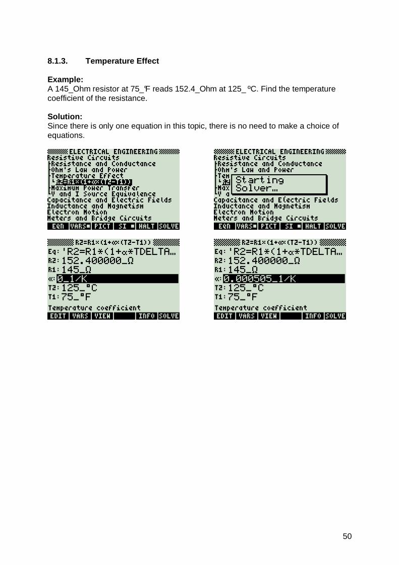
8.1.3. Temperature Effect Example: A 145_Ohm resistor at 75_°F reads 152.4_Ohm at 125_ ºC. Find the temperature coefficient of the resistance. Solution: Since there is only one equation in this topic, there is no need to make a choice of equations.

51

8.1.4. Maximum DC Power Transfer Example: A 12_V car battery has a resistive load of 0.52_Ohm. The battery has a source impedance of 0.078_Ohm. Find the maximum power deliverable from this battery and the power delivered to this resistive load. Solution: Upon examining the problem, equation 1, 2, 3 and 4 are needed to compute the solution for this problem.


52

8.1.5. V and I Source Equivalence Example: Find the short circuit current equivalent for a 5_V source with a 12.5_Ohm source resistance. Solution: Since there is only one equation in this topic, there is no need to make a choice of equations.

53

8.2. Capacitance and Electric Fields

8.2.6. Point Charge Example: A point charge of 14.5E-14_coulomb is located 2.4_m away from an instrument measuring electric field and absolute potential. The permittivity of air is 1.08. Compute the electric field and potential. Solution: Upon examining the problem, both equations are needed to solve this problem. Note that �0, the permittivity of free space does not appear as one of the variables that needs to be entered. It is entered automatically by the software, as it is a built in constant. However, �r, the relative permittivity must be entered as a known value.

54

8.2.7. Long Charged Line Example: An aluminum wire suspended in air carries a charge density of 2.75E-15_coulombs/m. Find the electric field 50_cm away. Assume the relative permittivity of air to be 1.04. Solution: Since there is only one equation in this topic, there is no need to make a choice of equations.

55

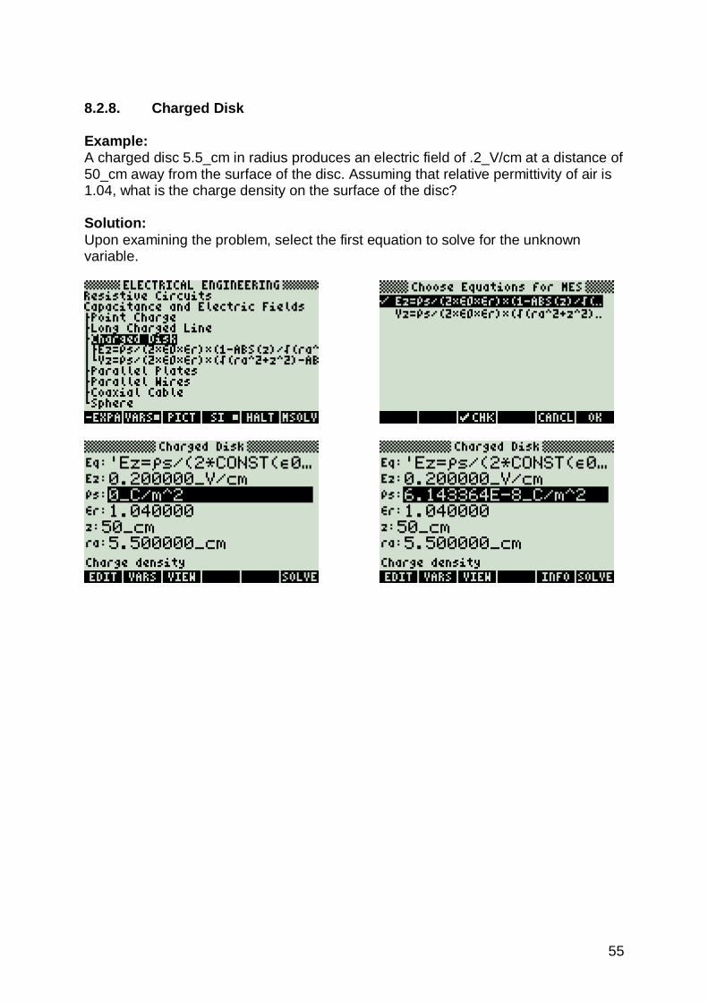
8.2.8. Charged Disk Example: A charged disc 5.5_cm in radius produces an electric field of .2_V/cm at a distance of 50_cm away from the surface of the disc. Assuming that relative permittivity of air is 1.04, what is the charge density on the surface of the disc? Solution: Upon examining the problem, select the first equation to solve for the unknown variable.

56

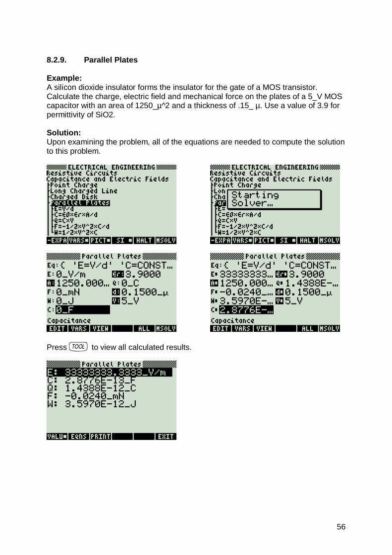
8.2.9. Parallel Plates Example: A silicon dioxide insulator forms the insulator for the gate of a MOS transistor. Calculate the charge, electric field and mechanical force on the plates of a 5_V MOS capacitor with an area of 1250_µ^2 and a thickness of .15_ µ. Use a value of 3.9 for permittivity of SiO2. Solution: Upon examining the problem, all of the equations are needed to compute the solution to this problem.


57

8.2.10. Parallel Wires Example: Compute the capacitance per unit length of a set of power lines 1_cm radius and 1.5_m apart. The dielectric medium separating the wires is air with a relative permittivity of 1.04. Solution: Since there is only one equation in this topic, there is no need to make a choice of equations.

58

8.2.11. Coaxial Cable Example: A coaxial cable with an inner cable radius of 0.3_cm and an outer conductor with an inside radius of 0.5_cm has a mica filled insulator with a permittivity of 2.1. If the inner conductor carries a linear charge of 3.67E-15_coulombs/m, find the electric field at the outer edge of the inner conductor and potential between the two conductors. Compute the capacitance per m of the cable. Solution: Upon examining the problem, all of the equations are needed to compute the solution to this problem.


59

8.2.12. Sphere Example: Two concentric spheres 2_cm and 2.5_cm radius, are separated with a dielectric with a relative permittivity of 1.25. The inner sphere has a charge of 1.45E-14_coulombs. Find the potential difference between the two spherical plates of the capacitor as well as the capacitance. Solution: Upon examining the problem, equations 1 and 3 are needed to compute a solution.

60

8.3. Inductors and Magnetism

8.3.1. Long Line Example: An overhead transmission line carries a current of 1200_A at 10_m away from the surface of the earth. Find the magnetic field at the surface of the earth. Solution: Since there is only one equation in this topic, there is no need to make a choice of equations.

61

8.3.2. Long Strip Example: A strip transmission line 2_cm wide carries a current of 16025_A/m. Find the magnetic field values 1_m away and 2_m from the surface of the strip. Solution: Upon examining the problem, both equations need to be used to compute the solution.

62

8.3.3. Parallel Wires Example: A pair of aluminum wires 1.5_cm in diameter are separated by 1_m and carry currents of 1200_A and 1600_A in opposite directions. Find the force of attraction, the magnetic field generated midway between the wires and the inductance per unit length resulting from their proximity. Solution: Upon examining the problem, equations 1 and 2 and 3 are needed to compute a solution.


63

8.3.4. Loop Example: Calculate the torque and inductance for a rectangular loop of width 7_m and length 5_m, carrying a current of 50_A, separated by a distance of 2_m from a wire of infinite length carrying a current of 30_A. The loop angle of incidence is 5 degrees relative to the parallel plane intersecting the infinite wire. Solution: Upon examining the problem, the last two equations are needed.


64

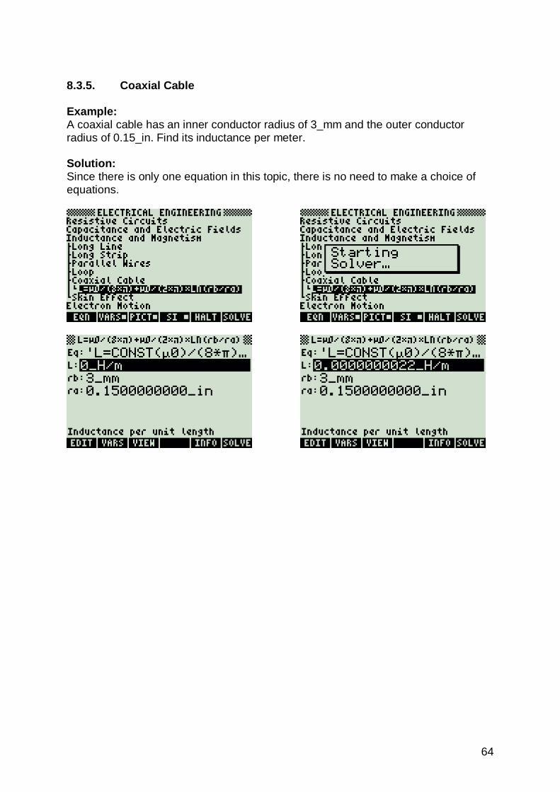
8.3.5. Coaxial Cable Example: A coaxial cable has an inner conductor radius of 3_mm and the outer conductor radius of 0.15_in. Find its inductance per meter. Solution: Since there is only one equation in this topic, there is no need to make a choice of equations.

65

8.3.6. Skin Effect Example: Find the effect on depth of signal penetration for a 100 MHz signal in copper with a resistivity of 6.5E-6 _Ohm*cm. The relative permeability of copper is 1.02. Solution: Upon examining the problem, both equations need to be used to compute the solution.

66

8.4. Inductors and Magnetism

8.4.1. Electron Beam Deflection Example: An electron beam in a CRT is subjected an accelerating voltage of 1250_V. The screen target is 40_cm away from the center of the deflection section. The plate separation is 0.75_cm and the horizontal path length through the deflection region is 0.35 cm. The deflection region is controlled by a 100_V voltage. A magnetic field of 0.456_T puts the electrons in the beam in a circular orbit. What is the vertical deflection distance of the beam when it reaches the CRT screen? Solution: Upon examining the problem, the first three equations are needed to solve this problem.


67

68

8.4.2. Thermionic Emission Example: A cathode consists of a cesium coated tungsten with a surface area of 2.45_cm^2. It is heated to 1200_°K in a power vacuum tube. If the Richardson's constant is 120_A/(m^2*K^2) and the work function is 1.22_V, find the current available from such the cathode. Solution: Since there is only one equation in this topic, there is no need to make a choice of equations.

69

8.4.3. Photoemission Example: A red light beam with a frequency of 1.4E14_Hz, is influencing an electron beam to overcome a barrier of 0.5_V. What is the electron velocity and find the threshold frequency of the light. Solution: Upon examining the problem, both equations need to be used to compute the solution.

70

8.5. Meters and Bridge Circuits

8.5.1. Amp, Volt, Ohmmeter Example: What resistance can be added to a voltmeter with a current sensitivity of 10 mA and a voltage sensitivity of 5 V to read 120 V? Solution: Upon examining the problem, the second equation needs to be selected to solve this problem.

71

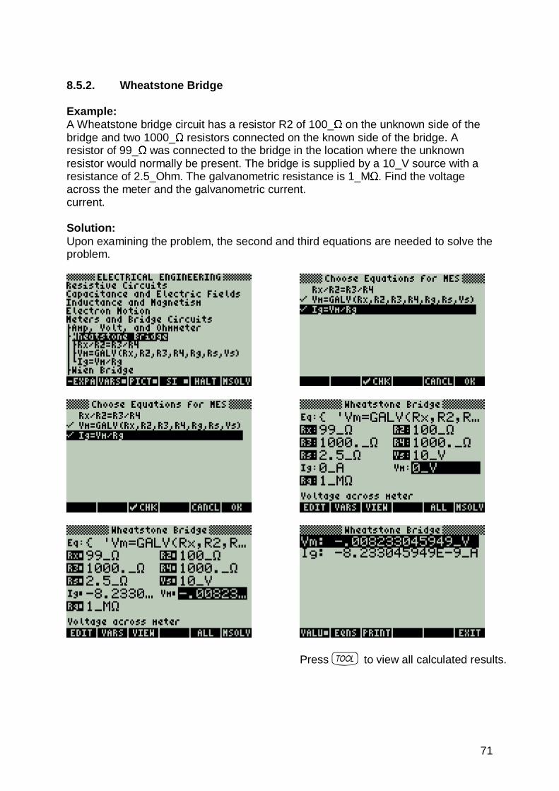
8.5.2. Wheatstone Bridge Example: A Wheatstone bridge circuit has a resistor R2 of 100_

� on the unknown side of the

bridge and two 1000_�

resistors connected on the known side of the bridge. A resistor of 99_

� was connected to the bridge in the location where the unknown

resistor would normally be present. The bridge is supplied by a 10_V source with a resistance of 2.5_Ohm. The galvanometric resistance is 1_M

�. Find the voltage

across the meter and the galvanometric current. current. Solution: Upon examining the problem, the second and third equations are needed to solve the problem.


72

8.5.3. Wien Bridge Example: A set of measurements obtained using a Wien bridge is based on the following input. All measurements are carried out at 1000_Hz. The known resistors R1 and R3 are 100_

� each, the series resistance is 200_

� and Cs is 1.2_µF. Find the values of the

unknown RC circuit components and the radian frequency. Solution: Upon examining the problem, the first, third and fifth equations are needed to solve the problem.


73

8.5.4. Maxwell Bridge Example: Find the inductance and resistance of an inductive element using the Maxwell bridge. The bridge resistors are 1000_

� each with a 0.22_µF capacitor and 470_

� parallel

resistance. Compute Lx and Rx. Solution: Upon examining the problem, the first two equations are needed to solve the problem.


74

8.5.5. Owen Bridge Example: A lossy inductor is plugged into an Owen bridge to measure its properties. The resistance branch has 1000_

� resistors and a capacitor of 2.25_µF on the non-

resistor leg and 1.25_µF capacitor on the resistor leg of the bridge. A series resistance of 125_

� connects the C4 leg to balance the inductive element.

Solution: Both equations are needed for solving the problem.


75

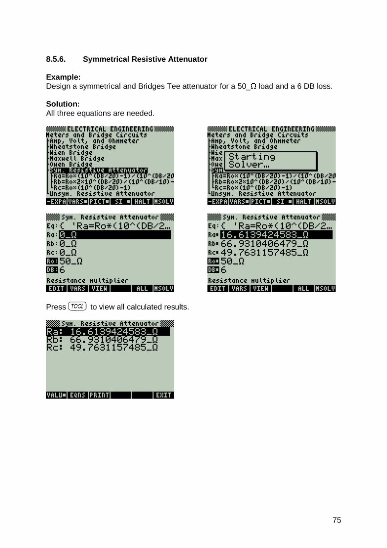
8.5.6. Symmetrical Resistive Attenuator Example: Design a symmetrical and Bridges Tee attenuator for a 50_

� load and a 6 DB loss.

Solution: All three equations are needed.


76

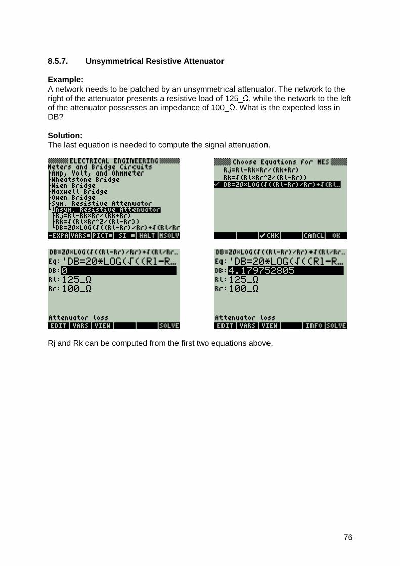
8.5.7. Unsymmetrical Resistive Attenuator Example: A network needs to be patched by an unsymmetrical attenuator. The network to the right of the attenuator presents a resistive load of 125_

�, while the network to the left

of the attenuator possesses an impedance of 100_�

. What is the expected loss in DB? Solution: The last equation is needed to compute the signal attenuation.

Rj and Rk can be computed from the first two equations above.

77

8.6. RL and RC Circuits

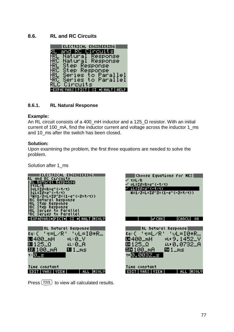
8.6.1. RL Natural Response Example: An RL circuit consists of a 400_mH inductor and a 125_

� resistor. With an initial

current of 100_mA, find the inductor current and voltage across the inductor 1_ms and 10_ms after the switch has been closed. Solution: Upon examining the problem, the first three equations are needed to solve the problem. Solution after 1_ms


78

Solution after 10_ms


79

8.6.2. RC Natural Response Example: An RC circuit consists of a 1.2_µF capacitor and a 47_

� resistor. The capacitor has

been charged to 18_V. A switch disconnects the energy source. Find the voltage across the capacitor 100_ms later. How much energy is left in the capacitor? Solution: Upon examining the problem, all of the equations are needed to solve the problem.


80

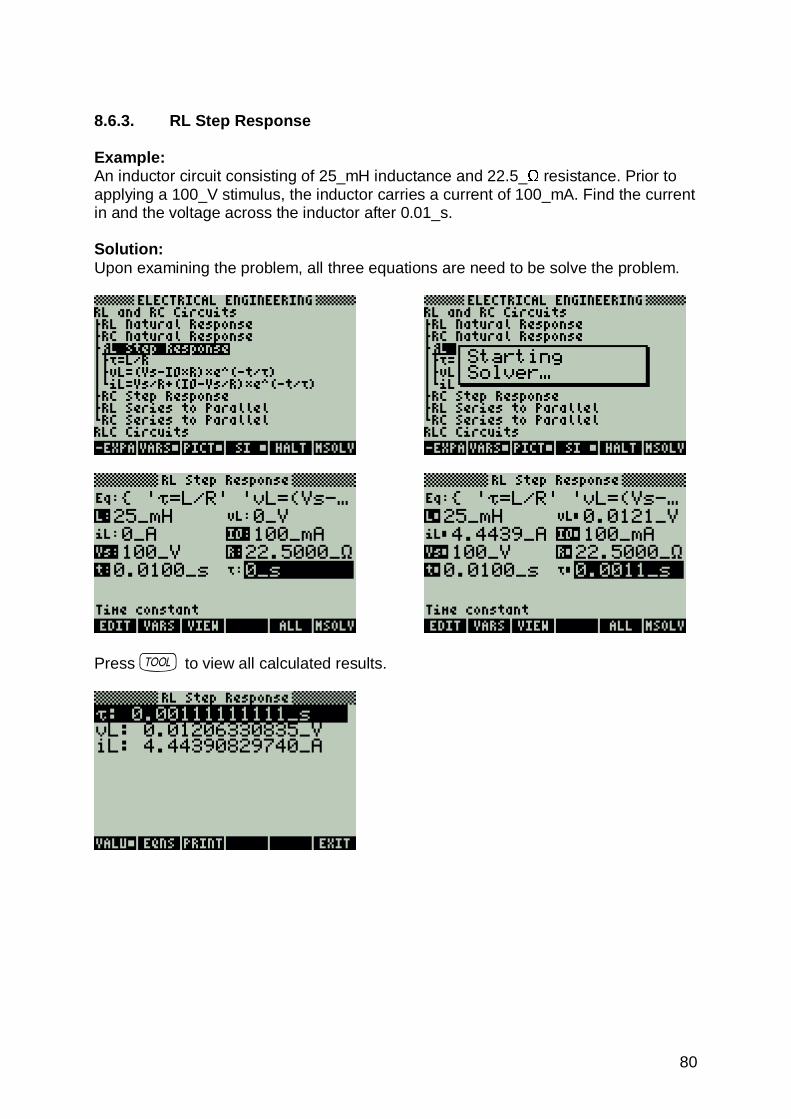
8.6.3. RL Step Response Example: An inductor circuit consisting of 25_mH inductance and 22.5_

� resistance. Prior to

applying a 100_V stimulus, the inductor carries a current of 100_mA. Find the current in and the voltage across the inductor after 0.01_s. Solution: Upon examining the problem, all three equations are need to be solve the problem.


81

8.6.4. RC Step Response Example: A 10_V step function is applied to an RC circuit with a 7.5_

� resistor and a 67_nF

capacitor. The capacitor was charged to an initial potential of -10_V. What is the voltage across the 0.1_ms after the step function has been applied? Solution: All three equations are needed to compute the solution for this problem.


82

8.6.5. RL Series to Parallel Example: A 24_mH inductor has a quality factor of 5 at 10000_Hz. Find its series resistance and the parallel equivalent circuit parameters. Solution: Upon examining the problem, the first six equations need to be solved as a set.


83

8.6.6. RC Series to Parallel Example: A parallel RC Circuit consists of a 47_µF and 150_k

� at 120_kHz.

Find its series equivalent. Solution: Upon examining the problem, equations 1, 3, 4, 6 and 7 are needed to solve the problem.


84

8.7. RLC Circuits

8.7.1. Series Impedance Example: A circuit consists of a 50_

� resistor in series with a 20_mH inductor and 47_µF

capacitor. At a frequency of 1000_Hz calculate the impedance and phase angle of impedance. Solution: All of the equations are needed to compute the solution for this problem.


85

8.7.2. Parallel Admittance Example: A parallel RLC Circuit consists of a 10 k

� resistor, 67 µH and 0.01 µF.

Find the circuit admittance parameters at a frequency of 10 MHz. Solution: All of the equations are needed to compute the solution for this problem.


86

8.7.3. RLC Natural Response Example: A RLC circuit consists of a 50_

� resistor in series with a 20_mH inductor and 47_µF

capacitor. Calculate the circuit parameters. Solution: All of the equations are needed to solve the parameters from these given set of variables.


87

8.7.4. Underdamped Transient Example: A parallel RLC circuit is designed with a 1_k

� resistor, a 40_mH inductor and a 2_µF

capacitor. The initial current in the inductor is 10_mA and the initial charge in the capacitor is 2.5_V. Calculate the resonant frequency and the voltage across the capacitor 1_µs after the input stimulus has been applied. Solution: All of the equations need to be selected to solve this problem.


88

8.7.5. Critical-Damped Transient Example: A critically damped RLC circuit consists of a 100_

� resistor in series with a 40_mH

inductor and a 1_µF capacitor. The initial inductor current is 1_mA and the initial capacitor charge is 10_V. Find the voltage across the capacitor after 10_µs. Solution: All of the equations are needed to compute the solution for this problem.


89

8.7.6. Overdamped Transient Example: An overdamped RLC circuit consists of a 10_

� resistor in series with a 40_mH

inductor and a 1_µF capacitor. If the initial inductor current is 0_mA and the capacitor is charged to a potential of 5_V, find the voltage across the capacitor after 1_ms. Solution: All of the equations are needed to compute the solution for this problem.


90

8.8. AC Circuits

8.8.1. RL Series Impedance Example: An RL circuit consists of a 50_

� resistor and a 0.025_H inductor. At a frequency of

400 Hz, the current amplitude is 24_mA. Find the impedance of the circuit and the voltage drops across the resistor and inductor after 100 ms. Solution: All of the equations are needed to compute the solution for this problem.


91

8.8.2. RC Series Impedance Example: An RC circuit consists of a 100_

� resistor in series with a 47_mF capacitor. At a

frequency of 1500_Hz, the current peaks at an amplitude of 72_mA. Find all the parameters of the RC circuit and the voltage drop after 150_µs. Solution: Use all of the equations to compute the solution for this problem.


92

8.8.3. Impedance � Admittance Example: Find the admittance of an impedance consisting of a resistive part of 125_

� and a

reactance part of 475_�

. Solution: All of the equations are needed to compute the solution for this problem.


93

8.8.4. Two Impedances in Series Example: Two impedances, consisting of resistances of 100_

� and 75_

� and reactive

components 75_�

and -145_�

respectively, are connected in series. Find the magnitude and phase angle of the combination. Solution: All of the equations are needed to compute the solution for this problem.


94

8.8.5. Two Impedances in Parallel Example: For two impedances in parallel possessing values identical to the previous example, calculate the magnitude and phase of the combination (resistances of 100_

� and

75_�

and reactive components 75_�

and -145_�

respectively). Solution: All of the equations are needed to compute the solution for this problem.


95

8.9. Polyphase Circuits

8.9.1. Balanced

� Network

Example: Given a line current of 25_A, a phase voltage of 110 V and a phase angle of 0.125_rad, find the phase current, power, total power and line voltage. Solution: Upon examining the problem, all equations are needed.


96

8.9.2. Balanced Wye Network Example: Using the known parameters in the previous example for the Balanced � Network, find the phase current, power, total power and line voltage (current of 25_A, a phase voltage of 110 V and a phase angle of 0.125_rad). Solution: All of the equations are needed to compute the solution for this problem.


97

8.9.3. Power Measurements Example: Given a line voltage of 110_V and a line current of 25_A and a phase angle of 0.1_rad, find the wattmeter readings in a 2 wattmeter meter system. Solution: All of the equations are needed to compute the solution for this problem.


98

8.10. Electrical Resonance

8.10.1. Parallel Resonance I Example: Calculate the resonance parameters of a parallel resonant circuit containing a 10,000_

� resistor, a 2.4_µF capacitor and a 3.9_mH inductor. The amplitude of the

current is 10_mA at a radian frequency of 10,000 rad/s. Solution: All of the equations are needed to compute the solution for this problem.


99

8.10.2. Parallel Resonance II Example: A parallel resonant circuit has a 1000_

� resistor and a 2.4_µF capacitor. The Quality

Factor for this circuit is 24.8069. Find the band-width, damped and resonant frequencies. Solution: All of the equations are needed to compute the solution for this problem.


100

8.10.3. Resonance in Lossy Inductor Example: A power source with an impedance Rg of 5_

� is driving a parallel combination of a

lossy 40_µH inductor with a 2_�

loss resistance, and a capacitor of 2.7_µF. Find the frequency of resonance and the frequency for maximum amplitude. Solution: Upon examining the problem, all equations are needed to solve for a solution.


101

8.10.4. Series Resonance Example: Find the characteristic parameters of a series-resonant circuit with R = 25_

�, L = 69_µH, C = 0.01_µF and a radian frequency of 125000 rad/s.

Solution: Upon examining the problem, all equations are needed to solve the problem.


102

8.11. OpAmp Circuits

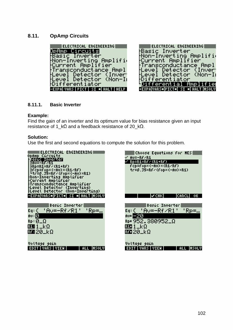
8.11.1. Basic Inverter Example: Find the gain of an inverter and its optimum value for bias resistance given an input resistance of 1_k

� and a feedback resistance of 20_k

�.

Solution: Use the first and second equations to compute the solution for this problem.

103

8.11.2. Non-Inverting Amplifier Example: Find the DC gain of a non-inverting amplifier with a feedback resistance of 1_M

� and

a resistance to the load of 18_k�

. Find the gain and the optimum value for a bias resistor. Solution: Use the first and second equations to compute the solution for this problem.

104

8.11.3. Current Amplifier Example: A current amplifier with a 200_k

� feedback resistance has a voltage gain of 42. If the

source resistance is 1_k�

, the load resistance is 10_k�

and the output resistance of the OpAmp is 100_

�.

Find the current gain, input and output resistances. Solution: Use all of the equations to compute the solution for this problem.


105

8.11.4. Transconductance Amplifier Example: Find the transconductance and output resistance for a transconductance amplifier with a voltage gain of 48 and an external resistance of 125_

�.

Solution: Upon examining the problem, all equations are needed to solve the problem.

106

8.11.5. Level Detector (Inverting) Example: An inverting level detector possesses two zener diodes to set the trip level. The setting levels are 4_V and 3_V, respectively, for the first and second diodes. The reference voltage is 5_V, the OpAmp is supported by a 10_k

� bias resistor and

a 1_M�

feedback resistor. Find the hysteresis, the upper and lower detection thresholds, and the input resistance. Solution: Upon examining the problem, all equations are needed to solve the problem.


107

8.11.6. Level Detector (Non-Inverting) Example: For a non-inverting level detector with the same specifications as the inverting level detector in the previous example, compute the hysteresis, the upper and lower detection thresholds, and the input resistance. Solution: Upon examining the problem, all equations are needed to solve the problem.


108

8.11.7. Differentiator Example: A differentiator circuit designed with an OpAmp has a slew rate of 1.5_V/µs. If the maximum output voltage is 5_V, and the feedback resistor is 39_k

�, what input

capacitor and resistor are needed for the amplifier with a characteristic frequency of 50_kHz? Solution: Use the third and fourth equations to compute the solution for this problem.


109

8.11.8. Differential Amplifier Example: Find the differential mode gain and the current gain for a differential amplifier with bridge resistors R1, R2, R3 and R4 of 10_k

�, 3.9_k

�, 10.2_k

� and 4.1_k

�,

respectively. Assume a voltage gain of 90. Solution: Use the third and fourth equations to compute the solution for this problem.


110

8.12. Solid State Devices

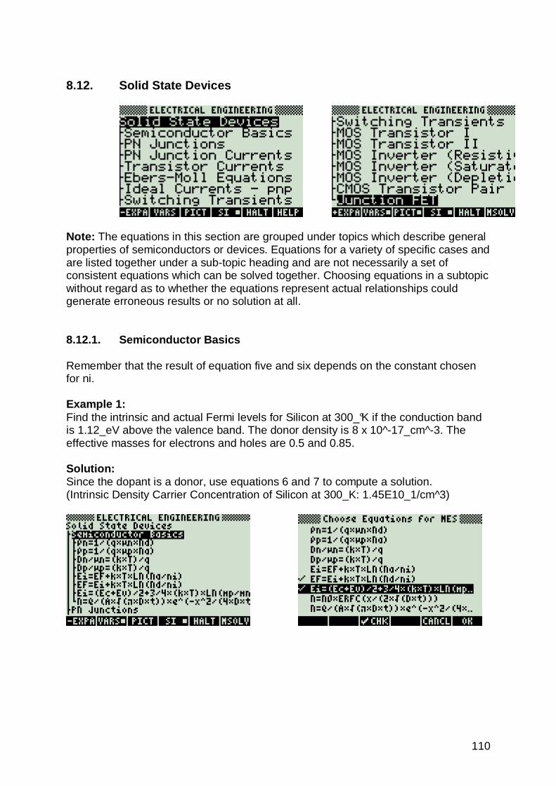
Note: The equations in this section are grouped under topics which describe general properties of semiconductors or devices. Equations for a variety of specific cases and are listed together under a sub-topic heading and are not necessarily a set of consistent equations which can be solved together. Choosing equations in a subtopic without regard as to whether the equations represent actual relationships could generate erroneous results or no solution at all. 8.12.1. Semiconductor Basics Remember that the result of equation five and six depends on the constant chosen for ni. Example 1: Find the intrinsic and actual Fermi levels for Silicon at 300_°K if the conduction band is 1.12_eV above the valence band. The donor density is 8 x 10^-17_cm^-3. The effective masses for electrons and holes are 0.5 and 0.85. Solution: Since the dopant is a donor, use equations 6 and 7 to compute a solution. (Intrinsic Density Carrier Concentration of Silicon at 300_K: 1.45E10_1/cm^3)

111


Example 2: Find the diffusion penetration depth after one hour for phosphorus atoms with a diffusion coefficient of 1.8 x 10^-14_cm^2/s. The carrier density at the desired depth is 8 x 10^17_1/cm^3 while the surface density is 4 x 10^19_1/cm^3. Solution: Equation 8 is needed to compute the solution for this problem.

112

8.12.2. PN Junctions Remember that the result of equation one and six depends on the constant chosen for ni. Example 1: A PN step junction is characterized by an acceptor doping density of 6 x 10^16_1/cm^3 and a donor doping density of 9 x 10^17_1/cm^3. The junction area is 100_µ^2 at room temperature. For an applied voltage of -5_V, find the built-in potential and junction capacitance. Use a value of 11.8 for the relative permittivity of silicon. Solution: Use the first five equations to compute the solution for this problem. (Intrinsic Density Carrier Concentration of Silicon at 300_K: 1.45E10_1/cm^3)


113

Example 2: A linearly graded junction has an area of 100_µ^2, a depletion layer width of 0.318005_µ, a built-in voltage of 0.8578_V and an applied voltage of -5_V. The relative permittivity of silicon is 11.8. Under room temperature conditions, what is the junction capacitance and the linear-graded junction parameter? Solution: Use the equations five and seven to compute the solution for this problem.


114

8.12.3. PN Junction Currents Example: A PN Junction is characterized as having a junction area of 100_µ^2, an applied voltage of 0.5_V, and diffusion coefficients for electrons and holes of 35_cm^2/s and 10_cm^2/s, respectively. The diffusion lengths for electrons and holes are 25_µ and 15_µ. The minority carrier densities are 5 x 10^6_1/cm^3 (electrons) and 25_1/cm^3 (holes). Find the junction current and the saturation current for room temperature conditions. Solution: Use the equations one and two or one and three to compute the solution for this problem.


115


116

8.12.4. Transistor Currents Example: A junction transistor has the following parameters: � is 0.98, the base current is 1.2_µA while ICBO is 1.8_pA. Find the �, emitter and collector currents. Solution: A few different choices are available, however the results might differ slightly due to the combination of equations used. The second, third and fifth equations can be used to solve this problem.


117

8.12.5. Ebers-Moll Equations Example: A junction transistor has a forward and reverse � of 0.98 and 0.10 respectively. The collector current is 10.8_mA while the forward current is 12.5_mA. respectively. Compute the base, saturation and reverse currents, in addition to the forward and the reverse b. Solution: The second through sixth equations are needed to solve this problem.


118

8.12.6. Ideal Currents - pnp Example: Find the emitter current gain � for a transistor with the following properties: base width of 0.75_µ, base diffusion coefficient of 35_cm^2/s, emitter diffusion coefficient of 12_cm^2/s, and emitter diffusion length of 0.35_µ. The emitter electron density is 30000_1/cm^3 and the base density is 500000_1/cm^3. Solution: Use the last equation to compute the solution for this problem.

119

8.12.7. Switching Transients Example: Find the saturation voltage for a switching transistor at room temperature when a base current of 5.1_mA is used to control a collector current of 20_mA. The forward and reverse �'s are 0.99 and 0.1 respectively. Solution: Use the last equation to solve this problem.

120

8.12.8. MOS Transistor I Remember that the result of equation one depends on the constant chosen for ni. Example: A p-type silicon with a doping level of 5 x 10^15_1/cm^3 has an oxide thickness of 0.01_µ and oxide charge density of 1.8 x 10^-10_C/cm^2. A -5_V bias is applied to the substrate which has a Fermi potential of 0.35_V. Assume the relative permittivity of silicon and silicon dioxide is 11.8 and 3.9, respectively, and the work function is 0.2_V. Solution: Use the second through last equations to compute the solution for this problem.


121

8.12.9. MOS Transistor II Example: An nMOS transistor has a 6_µ width and 1.25_µ gate length. The electron mobility is 500 cm^2/(V*s). The gate oxide thickness is 0.01_µ. The oxide permittivity is 3.9. The zero bias threshold voltage is 0.75_V. The bias factor is 1.1_V^1/2. The drain and gate voltages are 5_V and the substrate bias voltage is -5_V. Assuming that

� is 0.05_1/V and �F is 0.35_V, find all the relevant performance

parameters. Solution: Use all of the equations to compute the solution for this problem.


122

8.12.10. MOS Inverter (Resistive Load) Example: Find the driver device constant, output and mid-point voltages for a MOS inverter driving a 100_k

� resistive load. Driver properties include a 3_µ wide gate, a length of

0.8_µ, Cox of 345313 pF/cm2. The electron mobility is 500 cm^2/(V*s), VIH = 2.8_V, VT = 1_V and VDD = 5_V. Solution: Use all of the equations to compute the solution for this problem. By examining the equations, it is clear that there is more than one solution. However, the root finding algorithm stops, after the first solution has been found. In this example VOH, VOL, VIH, Vo and VM have to be positive and between 0 and VDD.


123

In total, there are eight solutions for this example. Calculate the other solutions by providing adequate guess(es) through the variables for the root finding algorithm. Computed results: Solution 1 Solution 2

Solution 3 Solution 4



124

8.12.11. MOS Inverter (Saturated Load) Example: A MOS inverter with a saturated MOS transistor as its load. The driver has a length of 1_µ and a width of 6_µ while the load has a length of 3_µ and a width of 6_µ. The Fermi level for the substrate material is 0.35_V, a zero-bias threshold of 0.75_V. Assume a drain supply voltage of 5_V and an output voltage of 3.1_V. The electron mobility is 500_cm^2/(V*s), the oxide capacitance per unit area is 345313_pF/cm^2 and the bias factor is 0.5_V^1/2. Find the output high voltage, the input high voltage, and the threshold of the load device. Solution: Use equations one, two, three, four, six and seven in order to get a complete solution for the problem

125


126

8.12.12. MOS Inverter (Depletion Load) Example: A MOS inverter with a depletion mode transistor as the load has a driver transistor 5_µ wide and 1_µ long while the load is a depletion mode device with a zero-bias threshold of -4_V, 3_µ long and 3_µ wide. The Fermi level for the substrate material is 0.35_V, a zero-bias threshold of 1_V. Given an electron mobility of 500_cm^2/(V*s) and a depletion threshold of -4_V; for the load device, compute VOL and VTL when the output voltage is 2.5_V. Assume VOH to be 4_V and 0.5 for �, the oxide capacitance per unit area is 34500_pF/cm^2. Solution: The problem can be solved with the equations one, two, three and four.



127

8.12.13. CMOS Transistor Pair Example: Find the transistor constants for an N and P MOS transistor pair given: N transistor: WN=4_µ, lN=2_µ, µn=1250_cm^2/(V*s), Cox=34530_pF/cm^2, VTN=1_V P transistor: VTP= -1_V, Wp=10_µ, µp=200_cm^2/(V*s), lP=2_µ VDD=2_V, VIH=5_V Solution: The solution can be calculated by selecting the first four equations.


128

8.12.14. Junction FET Example: Find the saturation current when the drain current at zero bias is 12.5_µA, the gate voltage is 5_V and the pinch off voltage is 12 V. The channel width is 3_µ, use a value of 11.8 for the relative permittivity of silicon, for the donor density use a value of 1 x 10^16_cm^-3. The built-in voltage is 0,85_V and the gate voltage is -8_V Solution: Use the third equation to solve this problem.

129

8.13. Linear Amplifiers

8.13.1. BJT (Common Base) Example: A common base configuration of a linear amplifier has an emitter resistance of 35_

�,

collector and base resistances of 1_M�

and 1.2_k�

resistances, respectively. The load resistor is 10_k

�. If the source resistance is 50_

� and �0 is 0.93, find �0 and

the gains for this amplifier. Solution: All of the equations are needed to compute the solution for this problem.

130


131

8.13.2. BJT (Common Emitter) Example: A common base configuration of a linear amplifier has an emitter resistance of 35_

�,

collector and base resistances of 1_M�

and 1.2_k�

resistances, respectively. The load resistor is 1_k

� and the output resistance is 1_M

�.

If the source resistance is 50_�

and �0 is 0.93, find �0 and the gains for this amplifier. Solution: All of the equations are needed to compute the solution for this problem.


132

8.13.3. BJT (Common Collector) Example: An amplifier in a common collector configuration has a gain �0 of 0.99. The emitter, base and collector resistances are 25_

�, 1000_k

�, and 100000_M

� respectively.

The load resistor is 100_�

. If the source resistance is 25_�

find all the mid-band characteristics. Solution: All of the equations are needed to compute the solution for this problem.


133

8.13.4. FET (Common Gate) Example: A FET amplifier connected in a common gate mode has a load of 10_k

�. The

external gate resistance is 1_M�

and the drain resistance is 125_k�

. The transconductance is 1.6 x 10^-3_Siemens. Find the midband parameters. Solution: All of the equations are needed to compute the solution for this problem.


134

8.13.5. FET (Common Source) Example: Find the voltage gain of a FET configured as a common-source based amplifier. The transconcductance is 2.5 x 10^-3_Siemens, a drain resistance of 18_k

� and a load

resistance of 100_k�

. Find all the parameters for this amplifier circuit. Solution: All of the equations are needed to compute the solution for this problem.


135

8.13.6. FET (Common Drain) Example: Compute the voltage gain for a common-drain FET amplifier. The transconcductance is 5 x 10^-3_Siemens, a drain resistance of 25_k

� and a load resistance of 100_k

�.

Find all the parameters for this amplifier circuit. Solution: All of the equations are needed to compute the solution for this problem.


136

8.13.7. Darlington (CC-CC) Example: Transistors in a Darlington pair having a �0 value of 100 are connected to a load of 10_k

�. The emitter, base and source resistances are 25_

�, 1500_k

� and 1_k

�,

respectively. The external base resistance is 27_k�

. Solution: All of the equations are needed to compute the solution for this problem.


137

8.13.8. Darlington (CC-CE) Example: An amplifier circuit has a base, emitter, and load resistance of 1.5_k

�, 25_

�, and

10_k�

, respectively. The configuration has a value of �0 equal to 100. The source and collector resistances are 1_k

� and 100_k

�.

Find the voltage gain, input and output resistances. Solution: All of the equations are needed to compute the solution for this problem.


138

8.13.9. Emitter-Coupled Amplifier Example: An emitter coupled pair amplifier is constructed from transistors with �0=0.98. The emitter, base and collector resistances are 25_

�, 2_k

� and 56_k

�, respectively. If

the load resistance is 10_k�

, find the mid-band performance factors. Solution: All of the equations are needed to compute the solution for this problem.


139

8.13.10. Differential Amplifier Example: A differential amplifier pair has a transconductance of 0.005_Siemens, �0=0.98, �0=49. The external collector and external emitter resistances are 18_k

� and 10_k

�

respectively. If the emitter resistance is 25_�

and the base resistance is 2_k�

, find the common mode, differential resistance and gains. Solution: All of the equations are needed to compute the solution for this problem.


140

8.13.11. Source-Coupled JFET Pair Example: Find the gain parameters of a source-coupled JFET pair amplifier if the external drain resistance is 25_k

�, and the source resistance is 100_

�. The drain resistance is

12_k�

and the transconductance is 6.8 x 10^-3_Siemens. Solution: All of the equations are needed to compute the solution for this problem.


141

8.14. Class A, B and C Amplifiers

Note: The equations in this section are grouped under topics which describe general properties of semiconductors or devices. Equations for a variety of specific cases and are listed together under a sub-topic heading and are not necessarily a set of consistent equations which can be solved together. Choosing equations in a subtopic without regard as to whether the equations represent actual relationships could generate erroneous results or no solution at all. 8.14.1. Class A Amplifier Example: A Class A power amplifier is coupled to a 50_

� load through the output of a

transformer with a turn ratio of 2. The quiescent operating current is 60_mA, and the incremental collector current is 50_mA. The collector-to-admitter voltage swings from 6_V to 12_V. The supply collector voltage is 15_V. The maximum current is 110_mA. Find the power delivered and the efficiency of power conversion. Solution: All of the equations are needed to compute the solution for this problem.

142


143

8.14.2. Power Transistor Example: A power transistor has a common emitter current gain of 125. A 750_

� base

resistance is coupled to an external emitter resistance of 10_k�

. The ambient temperature is 75_°F and the thermal resistance of the unit is 10_°C/W. The power that needs to be dissipated is 12.5_W. The base emitter voltage is 1.25_V while ICBO is 1_mA. Find the junction temperature, collector current and the instability factor. Solution: We note from the equation set that IC is computed in three different ways. To make the calculations consistent given the data, we use equations 1, 2, 4 and 5 to solve for this problem.


144

8.14.3. Push-Pull Principle Example: Find the output power for a push-pull circuit with a collector voltage of 15_V and a load resistance of 50_

�. The push-pull transformer secondary winding amplifies

voltage by a factor of 2.5. Solution: Use the third equation to compute the solution for this problem.

145

8.14.4. Class B Amplifier Example: A Class B amplifier provides 5_W to an effective load of 50_

�. The collector voltage

is 25_V. If the peak current is 500_mA, find the average DC current and the efficiency of power conversion. Solution: Use the first, second, fourth and fifth equations to compute the solution for this problem.

146

8.14.5. Class C Amplifier Example: A Class C amplifier is supplying a tuned circuit, with a quality factor of 5. If the output voltage is 15_V and the power delivered is 75_W. Find the capacitive reactance of the circuit needed in the tank circuit. Solution: Use the second equation to compute the solution for this problem.

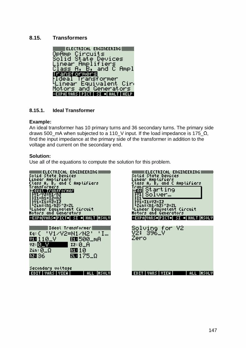
147

8.15. Transformers

8.15.1. Ideal Transformer Example: An ideal transformer has 10 primary turns and 36 secondary turns. The primary side draws 500_mA when subjected to a 110_V input. If the load impedance is 175_

�,

find the input impedance at the primary side of the transformer in addition to the voltage and current on the secondary end. Solution: Use all of the equations to compute the solution for this problem.

148


149

8.15.2. Linear Equivalent Circuit Example: The transformer in the above problem has a primary and secondary resistance of 18_

� and 5_

�, respectively. Therefore, the ideal transformer has 10 primary turns

and 36 secondary turns. The primary side draws 500_mA when subjected to a 110_V input. The corresponding coils have a reactance of 6_

� and 2.5_

�. The secondary

side is loaded with an impedance of 12.5_k�

. The reactive part of load is 10_�

Find the voltage and current on the secondary side in addition to the equivalent impedance on the primary side. Solution: Upon examining the problem, all of the equations are needed to compute the solution to this problem.


150

8.16. Motors and Generators

Note: The equations in this section are grouped under topics which describe general properties of semiconductors or devices. Equations for a variety of specific cases and are listed together under a sub-topic heading and are not necessarily a set of consistent equations which can be solved together. Choosing equations in a subtopic without regard as to whether the equations represent actual relationships could generate erroneous results or no solution at all. 8.16.1. Energy Conversion Example: A conductor having a length of 15_cm and a cross sectional area of 0.5_cm^2 is subjected to a magnetic induction of 1.8_T and a field intensity of 2.8_A/m. The magnetic reluctance is 0.46_A/Wb. The conductor has 32 turns and is moving at a rotational speed of 62_rad/s. Find the magnetic flux, the magnetic energy, the induced electric field and the mechanical pressure on the coil. Solution: All of the equations are needed to solve this problem.

151


152

8.16.2. DC Generator Example: A six-pole DC generator rotates at a mechanical speed of 31_rad/s. The armature sweeps across a flux of 0.65_Wb. There are eight parallel paths and 64 coils in the armature. The armature current is 12_A. The field is supplied by a 25_V source delivering a current of 0.69_A. Find the torque and the voltages generated in the armature. Solution: Upon examining the problem, equation one to six are needed to compute the solution for this problem.


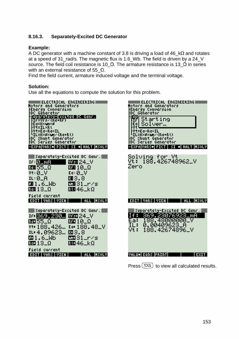
153

8.16.3. Separately-Excited DC Generator Example: A DC generator with a machine constant of 3.8 is driving a load of 46_k

� and rotates

at a speed of 31_rad/s. The magnetic flux is 1.6_Wb. The field is driven by a 24_V source. The field coil resistance is 10_

�. The armature resistance is 13_

� in series

with an external resistance of 55_�

. Find the field current, armature induced voltage and the terminal voltage. Solution: Use all the equations to compute the solution for this problem.


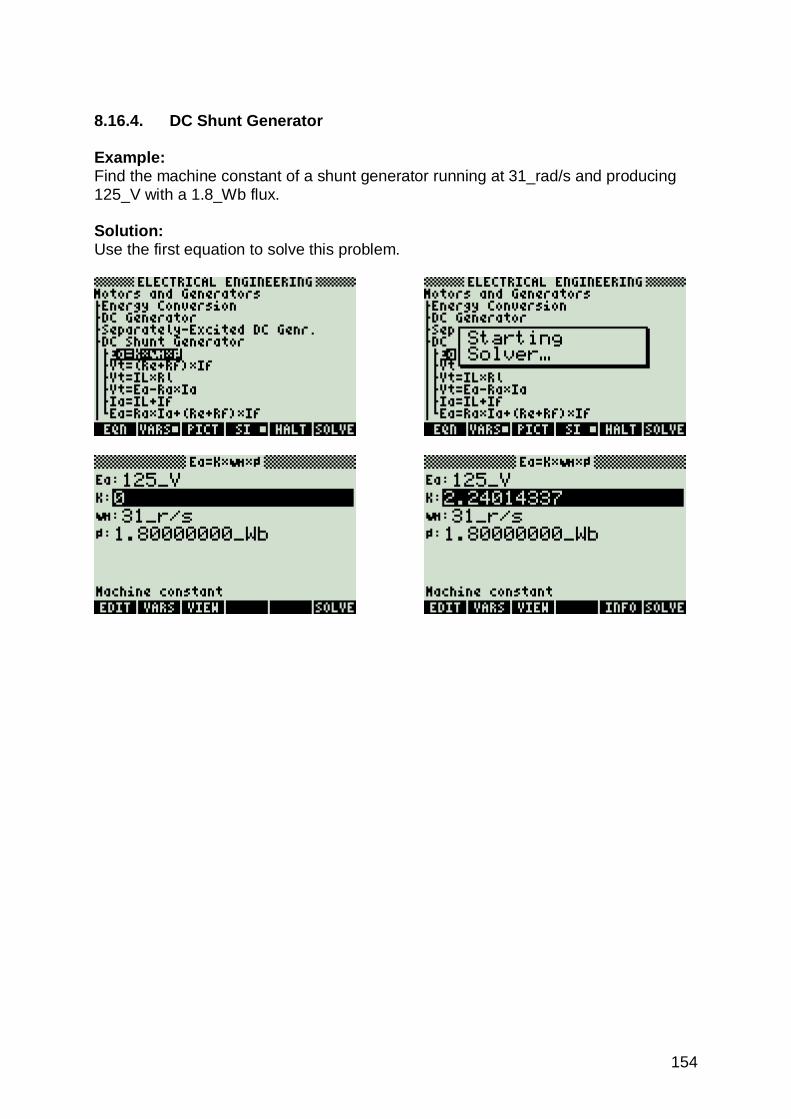
154

8.16.4. DC Shunt Generator Example: Find the machine constant of a shunt generator running at 31_rad/s and producing 125_V with a 1.8_Wb flux. Solution: Use the first equation to solve this problem.

155

8.16.5. DC Series Generator Example: Find the terminal voltage of a series generator with an armature resistance of 0.068_

� and a series resistance of 0.40_

�. The generator delivers a 15_A load

current from a generated voltage of 17_V. Solution: Use the second equation to solve this problem.

156

8.16.6. Separately-Excited DC Motor Example: Find the terminal voltage, field current and machine constant for a motor with an armature current 0.5_A and resistance of 100_

� rotating at an angular velocity of

31_rad/s. The back emf is 29_V. The field is driven by a 15_V source driving a 50_�

load. The flux available in the armature is 2.4_Wb. Solution: Solve the first, second, fourth and fifth equations to solve this problem.


157

8.16.7. DC Shunt Motor Example: Find the back emf for a motor with a machine constant of 2.1, rotating at 62_rad/s in a flux of 2.4_Wb. Solution: Use the fourth equation to solve this problem.

158

8.16.8. DC Series Motor Example: A series motor, with a machine constant of 2.4, rotating at 62_rad/s, is supplied with a terminal voltage of 110_V and produces a torque of 3_N*m. The armature resistance is 10_

�, the series resistance is 5_

�, and the adjustable resistance is

0.001_�

. Find the average voltage induced in the armature, the flux, and the load current. Solution: The first, third and fifth equations are needed to compute a solution.


159

8.16.9. Permanent Magnet Motor Example: Find the machine constant for a permanent motor rotating at 62.5_rad/s in a magnetic flux field of 1.26_Wb. Assume a 110_V back emf. Solution: The first equation is needed to compute the solution.

160

8.16.10. Induction Motor I Example: Find the mechanical power for an induction motor with a slip of 0.95, a rotor current of 75_A and a resistance of 1.8_

�.

Solution: Upon examining the problem, equation ten is needed to compute a solution.

161

8.16.11. Induction Motor II Example: An applied voltage of 125_V is applied to an eight pole motor rotating at 245_rad/s. The stator resistance and reactance is 8_

� and 12_

� respectively.

Find the maximum torque. Solution: Use the fourth equation to compute the solution.

162

8.16.12. Single-Phase Induction Motor Example: Find the forward slip for an eight pole induction motor with a stator frequency of 245_rad/s and a mechanical radian frequency of 62.5_rad/s. Solution: The first equation is needed to compute the solution.

163

8.16.13. Synchronous Machines Example: Find the stator radian frequency and the maximum torque for a synchronous machine with a mechanical rotational velocity of 31_rad/s. The motor has eight poles, a field current of 1.8_A and experiences an applied voltage of 130_V. Solution: The first and second equations are needed to compute the solution.


164

165

9. Used Keys The following keys are used by the TreeBrowser application, which provides the environment for Electrical Engineering. Keys while the TreeBrowser is active:

!+EXPA : opens a tree

!-EXPA : closes a tree

!!!!!EQN!!!! : shows the equation if there is something to show and if one is on the lowest level

!!!VARS!! : shows variables (if there are any)

!!!PICT!! : shows picture (if there is any)

!!!!!!SI!!!!!! : sets or clears the user flag for using units with SI units (user flag 60 and 61)

!!!ENGL!! : sets or clears the user flag for using units with English units (user flag 60 and 61)

!!!HELP!! : shows help for TreeBrowser

!!!HALT!! : temporary stops the TreeBrowser and gives access to the normal user stack. One has complete control over the calculator at this point. If an error happens by another program, for example, which is not covered by TreeBrowser your calculator may crash. The purpose of these functions is to allow simple calculations so that it is not necessary to leave TreeBrowser for this. ! = brings you back to the TreeBrowser.

!SOLVE : starts the solver if one is on the lowest level and the equation contains =. System flag 30 controls if the solver of the HP 48SX or the solver of the HP 48GX is used.

!MSOLV : starts the Multiple Equation Solver, all equations of the lowest level are grouped together. The equations should be related by topic to each other if you want usable results (also see user guide of the HP 48GX). ! = brings you back to the TreeBrowser.

™: double click opens or closes a tree G: starts the solver if the equation contains = H: toggles between the way equations are shown, if you provide a program

which tests system flag 13 it is possible to have two different appearances of the equation.

I: opens a choose box to select the equations which will be passed to the Multiple Equation Solver.

J: shows variables (if there are any) M: shows picture (if there is any) $: ends TreeBrowser `: opens or closes a tree

166

š—™˜: arrow keys to navigate or to move the screen @—: one page up @˜: one page down !—: first entry !˜: last entry @™: move screen to the right @š: move screen to the left V: choose font W: toggle fonts X: hide / show title Y: hide / show menu Z: integrated help Keys while an equation is shown: I: previous equation K: copies the current equation to the stack L: next equation W: toggles between big and small appearance of the equation (changes

system flag 80) $: leaves the equation view and jumps back to the TreeBrowser #: previous equation `: next equation š—™˜: arrow keys to navigate or to move the screen

167

10. Things To Do In principle, it would be possible to extend Electrical Engineering with more equations and/or more functionality. Contact me directly in this case to examine what would be needed for this. mailto:[email protected] Suggestions, criticism and/or improvements are welcome. 11. Version History 09.04.2012 Version 1.0 First public version. 01.01.2014 Version 1.01 Revised all equations. 01.12.2014 Version 1.10 Added Analysis. 12. Known Bugs Version 1.01 Revised all equations, added some missing

equations, fixed some bugs in some equations.

Documents

Library 1666: Electrical Engineering - bplacedsoftware49g.bplaced.net/EnglishSeite01/ElectricalEngineeringFor... · 7 4. Using the library Electrical Engineering is a fast and easy