Liberalization Agreements in the GATT/WTO and the Terms-of-trade

1

U.S. Patent and Trademark Office

OFFICE OF CHIEF ECONOMIST

Economic Working Paper Series

Liberalization Agreements in the GATT/WTO and the

Terms-of-trade Externality Theory: Evidence from Three

Developing Countries

Asrat Tesfayesus, Economist

USPTO Economic Working Paper No. 2016-3

June 2016

The views expressed are those of the individual authors and do not necessarily reflect official positions of the Office of

Chief Economist or the U. S. Patent and Trademark Office. USPTO Economic Working Papers are preliminary research

being shared in a timely manner with the public in order to stimulate discussion, scholarly debate, and critical comment.

For more information about the USPTO’s Office of Chief Economist, visit www.uspto.gov/economics.

http://www.uspto.gov/economics

June 1, 2016 10:31 Accepted for publication at Review of Int. Econ. ”Working Paper”

1

RESEARCH ARTICLE

Liberalization Agreements in the GATT/WTO and the

Terms-of-trade Externality Theory: Evidence from Three

Developing Countries.

Tesfayesus†

(June 2016)

The terms-of-trade theory suggests that governments engage in trade negotiations with theirtrade partners in an effort to escape from a terms-of-trade prisoner’s dilemma by mutuallyinternalizing externalities that they impose on each other. In this paper, I use predictions ofthe terms-of-trade relationship to provide support for the theory based on the negotiatingpatterns of three developing countries during the Uruguay Round of the Generalized Agree-ments on Tariff and Trade. I use industry level import value as well tariff schedules from thesecontracting party states that were graduated from the U.S. Generalized System of Preferenceslist during the Uruguay Round. I exploit the rapid change in their tariff schedules from thebest response to the optimal level within a single negotiation round to empirically test theterms-of-trade theory. I find that my estimates are consistent with the predictions of the the-ory as applied to these three developing countries that were compelled to negotiate for tariffconcessions during the Uruguay Round. (JEL F11, F13)

Keywords: Developing Countries, Multilateral Agreements, Tariffs, Terms-of-trade

Table of Contents

1. Introduction

2. Terms-of-trade Theory2.1. Terms-of-trade Theory:

Literature Review2.1. Terms-of-trade Theory: Model

3. Identification Strategy

4. Data Description4.1. Import Data4.2. Tariff Data4.3. Data Used in Regression Analysis

5. Results

6. Conclusion

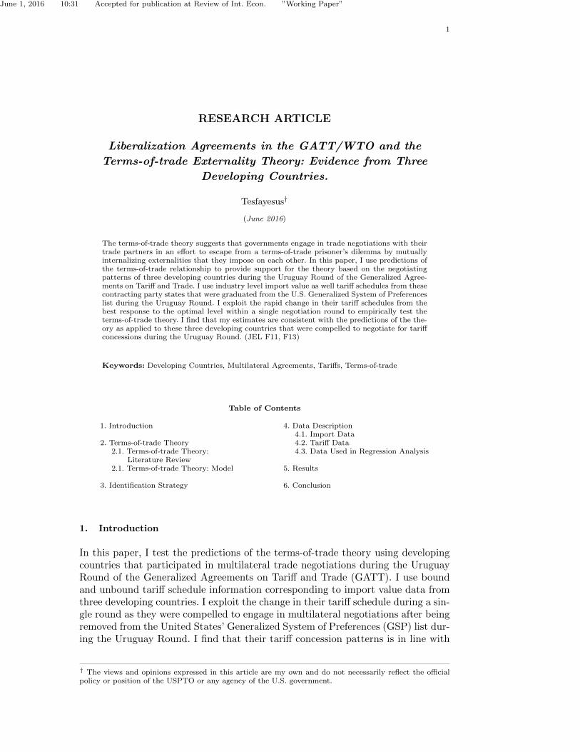
1. Introduction

In this paper, I test the predictions of the terms-of-trade theory using developingcountries that participated in multilateral trade negotiations during the UruguayRound of the Generalized Agreements on Tariff and Trade (GATT). I use boundand unbound tariff schedule information corresponding to import value data fromthree developing countries. I exploit the change in their tariff schedule during a sin-gle round as they were compelled to engage in multilateral negotiations after beingremoved from the United States’ Generalized System of Preferences (GSP) list dur-ing the Uruguay Round. I find that their tariff concession patterns is in line with

† The views and opinions expressed in this article are my own and do not necessarily reflect the officialpolicy or position of the USPTO or any agency of the U.S. government.


2 Tesfayesus

the predictions of the terms-of-trade theory. Accordingly, this paper contributes towhat is still a very lacking empirical literature addressing a long standing questionabout what trade negotiators negotiate about.

It is apparent that the participant nations’ main objective in creating the GATTand, subsequently, the WTO system is to have an international forum to liberal-ize trade. However, what they actually negotiate about in how to share the pieof the gains from more liberal trade is not immediately obvious. According to theterms-of-trade prisoner’s dilemma theory, countries negotiate to remove barriers totrade as a way to internalize externalities that they impose on each other. In otherwords, nations use international trade institutions as a forum to negotiate conces-sions that will enable them to escape from a terms-of-trade prisoner’s dilemma. Assuch, they are able to reciprocally reduce inefficiencies that are a consequence ofbarriers to trade as well as reap the benefits of engaging in more trade. While thistheoretical framework that provides a basis for multilateral trade negotiations iswell developed, the empirical literature in support of this hypothesis significantlylags behind. Furthermore, none extends far back to the GATT years to study therelevance of this theory as it applies to earlier rounds of negotiations.

In this paper, I use disaggregated data from three developing countries (i.e.Brunei, Paraguay, and South Korea) that participated in the Uruguay Round tradenegotiations under GATT in order to test the terms-of-trade theory. Prior to theUruguay Round, these countries were granted preferential treatment as GSP ben-eficiaries and were not required to accord reciprocal tariff reduction concessions toother GATT contracting members. Thus, they were in a position to set their tariffschedule according to the social planner’s utility maximization solely as a func-tion of payoff to domestic constitutents. This is referred to as the best responsetariff. During the Uruguay Round, however, these countries were graduated fromthe U.S.’s GSP list and were compelled to engage in multilateral negotiations toreciporcally reduce their tariff barriers. Their tariff schedule subsequent to thesenegotiations, also referred to as the politically optimal tariff, are set as the opti-mal level of concessions taking both domestic constiutents’ and trading partners’interest into account.

The fact that these countries went from their best response tariff level to thepolitcally optimal within a short period of time during a single negotiation roundprovides a natural experiment environment to test the terms-of-trade theory. Us-ing disaggregated data on both import value and the difference in tariff schedulesbefore and after the Uruguay Round, I am able to test if the tariff concesssionpatterns for these three countries are consistent with the predictions of the terms-of-trade theory. More specifically, I take to the data the prediction that the boundtariff level will be set lower relative to the unbound level as the pre-negotiationimport value for a given product is higher. I find that my estimates are consistentwith these predictions of the terms-of-trade relationship and are statistically signif-icant at various levels of industry fixed-effect disaggregations. Furthermore, whenI introduce a country-industry fixed-effect, the results persist and are statisticallysignificant on the full sample. Results at the individual country level are also inline with the terms-of-trade theory predictions, while the results at the individualindustry level are mixed and inconclusive.

Consistent with the terms-of-trade theory, my findings suggest that some devel-oping countries do in fact have trade matters to negotiate about in the internationaltrade negotiation forum and mutually benefit from an agreement. Furthermore, inlight of the fact that all parties have something to negotiate about, this findingmay give additional weight to the pressing question about why the Doha Roundremains stagnant.


3

The remainder of this paper is organized as follows. In Section 2, first, I explainthe terms-of-trade theory, as articulated in the literature. Secondly, I present themodel, a la Bagwell and Staiger (2011), with which they formulate a testablehypothesis. In Section 3, I explain how I use the model to test the theory thatcountries negotiate to escape from a terms-of-trade prisoner’s dilemma. In Section4, I provide a detailed description of the data, the empirical challenges they raise,and how I resolve them. In Section 5, I report my results. Finally, I conclude inSection 6.

2. Terms-of-trade Theory

2.1 Terms-of-trade Theory: Literature Review

One theoretical explanation for the existential purpose of international trade in-stitutions is for them to serve as a forum to mitigate the terms-of-trade prisoner’sdilemma that trading nations are faced with. 1 The origin of this theory datesback to Johnson (1954) in which the author notes that in the absence of tradeagreements, the import tariffs imposed and the trade wars that will ensue wouldlead countries to an inefficient trade protection equilibrium. Nations that are largeenough to affect world prices of a good they import can impose tariffs on suchimports to improve their terms-of-trade. In turn, their large country trading part-ners will impose retaliatory tariffs leading to a wash of any terms-of-trade gain.In effect, these countries are left with larger trade barriers that have significantdistortionary impact. Yet, none are able to benefit from a net terms-of-trade gain.Thus, the theory suggests, these countries resolved to pull themselves out fromsuch a lose-lose equilibrium by using international trade institutions as a forum tonegotiate and enter into mutually beneficial trade liberalization agreements. WhileMayer (1981) illustrated this point in a simple static game-theoretic framework,Grossman and Helpman (1995a) as well as Bagwell and Staiger (1999), which wasfurther developed in Bagwell and Staiger (2002), have argued that the result per-sists even in a more complicated environment where a government is faced withdomestic political pressure.

However, while Bagwell and Staiger (2011) make a great leap forward in providingevidence for the terms-of-trade theory, little empirical study has been done tryingto substantiate the terms-of-trade theory or shed more light in general on whatmember states negotiate about.2 Accordingly, in this paper, I focus on conductingan empirical exercise using import and tariff data from three developing countries totest the validity of the terms-of-trade prisoner’s dilemma theory. To do so, I exploitthe fact that these countries are GATT contracting parties and were engaged inmaking substantial tariff concessions during the Uruguay Round.

In order to do so, first it is instructive to note that the terms-of-trade theorysuggests that each country on the negotiating table has an economic influence in

1Other theories include the (1) commitment theory, Maggi and Rodriguez-Clare (2007), which argues thatgovernments enter into binding international trade because they value making strong level of liberalizationcommitments to their domestic private stakeholders (2) the relocation theory, Ossa (2011), which arguesthat trade negotiations could enable countries to internalize a ”production relocation externality”. Thelatter literature builds upon Krugman (1980) and Venables (1987) which help identify the productionrelocation effect of tariff as well as Baldwin and Robert-Nicoud (2000) which applies this mechanism to atrade agreement environment. Finally, Antras and Bagwell (2012), explain that cost-shifting mechanismsthrough offshoring introduce an additional layer of complexity in international trade agreemetns.2In their paper ’What Do Trade Negotiators Negotiate About? Empirical Evidence from the World TradeOrganization’, AER 2011, Bagwell and Staiger use data from 16 countries to test and validate the terms-of-trade theory by illustrating the fact that the magnitude of the negotiated decrease in tariffs for a givengood is proportional to its import volume. A more recent empirical contribution further substantiatingthis theory is Ludema and Mayda (2013).


4 Tesfayesus

international trade that gives them the leverage to effectively negotiate. The theoryaccentuates the point that large countries, defined as those that can influence worldprices of some goods that they import, will have exercised their ability to externalizecost to their trading partners through their tariff schedule choices. Thus, these largecountries that may have imposed externalities on each other can come to the tableto negotiate down their tariff schedules and internalize some of these costs. As such,they manage to reach a mutually more beneficial equilibrium. In other words, alarge country accords some ‘control’ over its tariff schedule to its trading partnerthat is also a large country. Hence, if the terms-of-trade theory indeed gives a solidaccount of what countries negotiate about, then we should expect to see moresignificant tariff cuts on goods in which the imposition of tariff-based externalitieson large countries is greatest.

In order to test this hypothesis, I make use of import and tariff data from boththe GATT and WTO years. I consider three developing countries that were markedoff the US GSP list and compelled to engage in any meaningful concessions for thefirst time during the Uruguay Round. Based on regression analyses using data fromthese countries, I provide results that are in line with the terms-of-trade prisoner’sdilemma hypothesis.

2.2 Terms-of-trade Theory: Model

In their model, Bagwell and Staiger (2011) demonstrate the theoretical relation-ship between changes in negotiation based tariff schedules on the one hand andthe import demand and export supply elasticities as well as import volumes on theother. The model exploits these relationships to identify negotiators’ goal of escap-ing from the terms-of-trade prisoner’s dilemma through their GATT/WTO tradeagreements. Here, I present the results from Bagwell and Staiger’s (2011) modelthat guides the terms-of-trade prisoner’s dilemma hypothesis testing methodolo-gies.

Bagwell and Staiger (2011) hypothesize that tariff based cost-shifting to export-ing trade partners is particularly salient when (i) the import demand elasticityis larger (ii) the export supply elasticity is smaller or (iii) the import volume islarger. In their theoretical framework, the authors produce a testable design of thishypothesis. First, the authors develop a structural design that exploits the relation-ship between negotiated tariff concession levels and import volumes. Subsequently,they reduce the model to a formulation with which one can test whether interna-tional trade negotiations aim to curtail tariff based cost-shifting to exporting tradepartners.

More specifically, Bagwell and Staiger (2011) derive a relationship betweenthe politically optimal tariff (τPO), the best response tariff (τBR), the numberof product level units that the country has imported (M(p(τBR, pwBR))), andthe best response world price (pwBR) for any given product. In developing theeconomic environment, the authors first assume that the tariff imposing countrieshave linear demand and supply curves. Furthermore, it is assumed that thegovernment puts a relatively higher weight on producer surplus when maximizingits welfare function. That is, the government’s politically optimal tariff scheduleis expected to be positive as it is influenced by its domestic producing sector’sprotectionist interest. In such an environment, with a possibility of non-reciprocaltariff negotiations they demonstrate that the following equation holds


5

τPO − τBR = β0 + (β1 − 1)τBR + β2[M(p(τBR, pwBR))

pwBR] (1)

For any given set of products with constant terms-of-trade level (i.e. r ≡ pwPO

pwBR =1, if a country’s political economy environment and the demand and supply elas-ticities are the same, Bagwell and Staiger (2011) explain that the terms-of-trade

theory predicts an estimated β1 > 0 and β2 < 0.

3. Identification Strategy

The hypothesis being tested is that the magnitude of the Most Favored Nation(MFN) based tariff reduction up to the post-negotiation bound level should belarger the higher the import volume for that particular good.3 If so, the theorythat countries negotiate to escape from the terms-of-trade prisoner’s dilemma isnot rejected.

The empirical design to test this hypothesis directly follows from equation (1),which, when rearranged, yields

τPO = β0 + β1τBR + β2[

M(p(τBR, pwBR))

pwBR] (2)

Thus, the estimating equation is as follows

τWTOgc = β0 + β1τ

BRgc + β2m

BRgc + εgc (3)

g refers to products indexed at the HS six-digit level, c refers to the negotiating

country imposing the tariff, mBR ≡[M(p(τBR,pwBR))

pwBR

], and εgc is the error term.

4. Data Description

The data that I use come from two main sources. For the disaggregated importdata and bound tariff information, I use the United Nations Commodity TradeStatistics Database (UN COMTRADE) and WTO’s Integrated database (IDB).Furthermore, I use the TRAINS (Trade Analysis and Information System) databasethat is maintained by the United Nations Conference on Trade and Development(UNCTAD) for both pre-negotiation and post-negotiation applied and bound tar-iff schedules. These sets of data are extracted from the World Integrated TradeSolution (WITS) as well as the WTO website directly.

3The MFN principle is stated in the first paragraph of the original GATT article and stipulates that ’anyadvantage, favour, privilege or immunity granted by any contracting party to any product originating inor destined for any other country shall be accorded immediately and unconditionally to the like productoriginating in or destined for the territories of all other contracting parties.’


6 Tesfayesus

4.1 Import Data

UN COMTRADE data, which goes as far back as 1962, provides import data forboth WTO member states and non-members at the country level for goods disag-gregated at as low as the six-digit Harmonized System (HS) level. The databaseprovides complete country level trading partner information. However, for the pur-pose of this study, it suffices to denote trading partners as the rest of WTO membercountries.

The WTO IDB database contains import value data for all products and tradepartners as reported by the importer and serves as the primary source of the tradedata used in this study.

4.2 Tariff Data

For the traded goods, the relevant tariff schedules I use are both pre-negotiation un-bound tariff levels that importing countries impose as well as their post-negotiationbound optimal tariff levels that in the model are referred to as the pre-negotiationbest response tariff levels and the post-negotiation optimal tariff, respectively.4 Tothe extent possible, the pre-negotiation unbound tariff collected are those levelsthat the importing country had imposed right before entering into any meaningfulconcession negotiation. As such, we can reasonably rule-out the likelihood that thedifferences in tariff schedules between the unbound and bound tariffs are driven byother changes in domestic or international economic dynamics.

Accordingly, in my analyses, I use data from the developing countries for whichI had sufficient observation from the earlier part of the 1990s in the advent of theUruguay Round completion. The pre-negotiation tariff schedule I use correspond tothe applied level tariffs disaggregated at the six-digit level; which I obtain from theUNCTAD maintained TRAINS database. Finally, information on the 1996 boundtariff level are extracted from the WTO’s IDB; which comprises both MFN appliedand bound tariff data of the HS classification disaggregated at the six-digit level.

4.3 Data Used in Regression Analysis

In the results that I report below, the baseline OLS model I estimate is mappeddirectly from equation (3) as follows:

τWTOgc = αg + αc + β1τ

BRgc + β2[V BR

gc ] + εgc (4)

where τBRgc indicates ad valorem tariff levels imposed on each product before con-

cession agreements are entered into during the Uruguay Round and τWTOgc indicates

the post agreement tariff levels. g refers to the product indexed at the HS six-digitlevel, while c identifies the negotiating country imposing the tariff. αg is the HSproduct level fixed effect for disaggregation ranging between the one-digit to thefour-digit level, while αc is a country fixed effect, included only for the full sampleestimate. Finally, V BR

gc is the pre-agreement import value of the traded goods inmillions of dollars, and εgc is the error term.

Bagwell and Staiger (2011) make use of 16 countries that joined the WTO so asto have a clean data in which countries immediately drop their best response tariff

4The post-negotiation bound tariff is presumed to be the optimal tariff based on the rationale that nu-merous rounds of negotiations in the GATT years have allowed contracting parties to gradually reach thetariff that will mutually maximize their gains from trade.


7

schedule to the optimal WTO level. For this set of countries, they find evidencethat the terms-of-trade theory does in fact play a significant role in the motivationfor engaging in trade negotiations.

I make use of the same analytical approach to test if the terms-of-trade theorywould still hold when applied to the three developing countries in my data thatunderwent significant tariff concessions during the Uruguay Round. By focusingon WTO entering countries, Bagwell and Staiger (2011) are able to avoid thegradual aspect of tariff concessions. Such a non-gradual drop in tariff concessions,while necessary for the analysis, rarely came about in the GATT years. In order tocircumvent this problem, I proceed as follows. First, I focus on countries designatedas developing countries and were granted GSP treatment by the United States.Subsequently, from this list of countries, I identify those that were taken off theGSP list by the US during the Uruguay Round and were compelled to negotiateand reduce their tariff barriers.

The countries that satisfy this stipulation are the following: Portugal, Romania,Hong Kong, Republic of Korea, Singapore, Paraguay, Bahrain, Brunei Darussalam,and Union of Myanmar. From this list of countries, I was able to obtain the neces-sary pre-WTO unbound tariff and trade data as well as the bound tariff data sub-sequent to the completion of the Uruguay Round for the following countries: HongKong, Republic of Korea, Singapore, Brunei Darussalam, and Paraguay. However,all of the unbound tariff for all products in Hong Kong are at 0 percent and virtu-ally all unbound tariff data for all imports in Singapore are at 0 percent. Therefore,I cannot use these two countries for my empirical study to test the terms-of-tradetheory within the framework of the model. I omit these two countries from myregression analysis. Thus, the analysis and results obtained are based on data ob-tained on the three remaining countries (i.e. Republic of Korea, Paraguay, andBrunei Darussalam). A more detailed information on the data from each countryis provided in Table 1-2 below. In addition to their removal from the GSP list,the fact that I use developing countries that are ex ante different allows me toconsider if the terms of trade theory can be extended to such heterogenous coun-tries. For instance, Brunei is an oil rich country and heavily relient on it whileSouth Korea was already experiencing high growth rates and is now considereda middle income country. Furthermore, the diversity in their geographic location,institutional structure and trade patterns may suggest that the findings are morebroadly applicable.

It should be noted that while there is some level of coordination with other de-veloped countries that have accorded GSP treatment (i.e. Japan, EU), it is unclearhow effectively it is executed. If there is failure of coordination my results shouldbe biased toward not finding support for the terms-of-trade theory. The fact thatI do find some evidence despite the possibility of such a failure is reassuring.

Another possible concern with this approach relates to the issue of the ostensi-ble fact that developing countries will inevitably have more to give to developedcountries when they come to the negotiating table after having been removed fromthe GSP list, in the unlikely event that they were previously accorded an uncon-ditional MFN treatment. The rationale for this assertion is that while developingcountries were getting a free ride by being on the GSP list, developed countriessuch as the US were making reciprocal concessions vis-a-vis other developed coun-tries and GSP non-beneficiaries. Thus, even once they are off the GSP list, theMFN benefits they have been getting for products not on the GSP list persists.However, the developing countries themselves have yet many concessions to giveas they have not engaged in any substantial liberalization previously.

Thus, the question is, other than the goods on the GSP list, how much more do


8 Tesfayesus

developed countries have to offer in terms-of-trade liberalization with which thesecountries newly off the GSP list are incentivized to reciprocate. First, those goodsremoved from the GSP list are the primary focus of this exercise. Second, the factthat the Uruguay Round opened-up numerous other aspects of trade liberaliza-tion, including agricultural products as well as the phasing-out of the Multi-FiberArrangement, has given developing countries additional concessions to potentiallybargain for and benefit from.

Finally, an omitted variable bias may be a concern in estimating the relationshipbetween negotiated tariff reductions and import volume; especially in light of thefact that removal from the GSP list is the basis of selection. More specifically, theremay be unobserved variables that affect both the countries’ importing and nego-tiation behavior simultaneously and specifically for the transition period duringwhich we observe the data. There may also be trend specific factors, such as coun-try or industry level growth, that may introduce biases. I address these concernsin multiple ways.

First, the import data is at a disaggregated industry level and originating frommultiple countries. Thus, the design is less likely to suffer from a bias based onthe origination of the import. Second, the periods of observation for imports aswell as both the pre and post negotiation tariffs are within a short period of time;the longest gap being four years. This approach allows for the exclusion of trendspecific variations and mitigates the risk that confounding factors are introducedin the transitioning period. Finally, I also control for unobserved characteristicsthat may introduce cross country or industry variations in the estimation results.To do so, first, I use country and industry fixed effects in the overall results that Ipresent. Second, I report the results both at the individual country and industrylevels separately. As explained in detail below, most of the results are robust tothese variations.

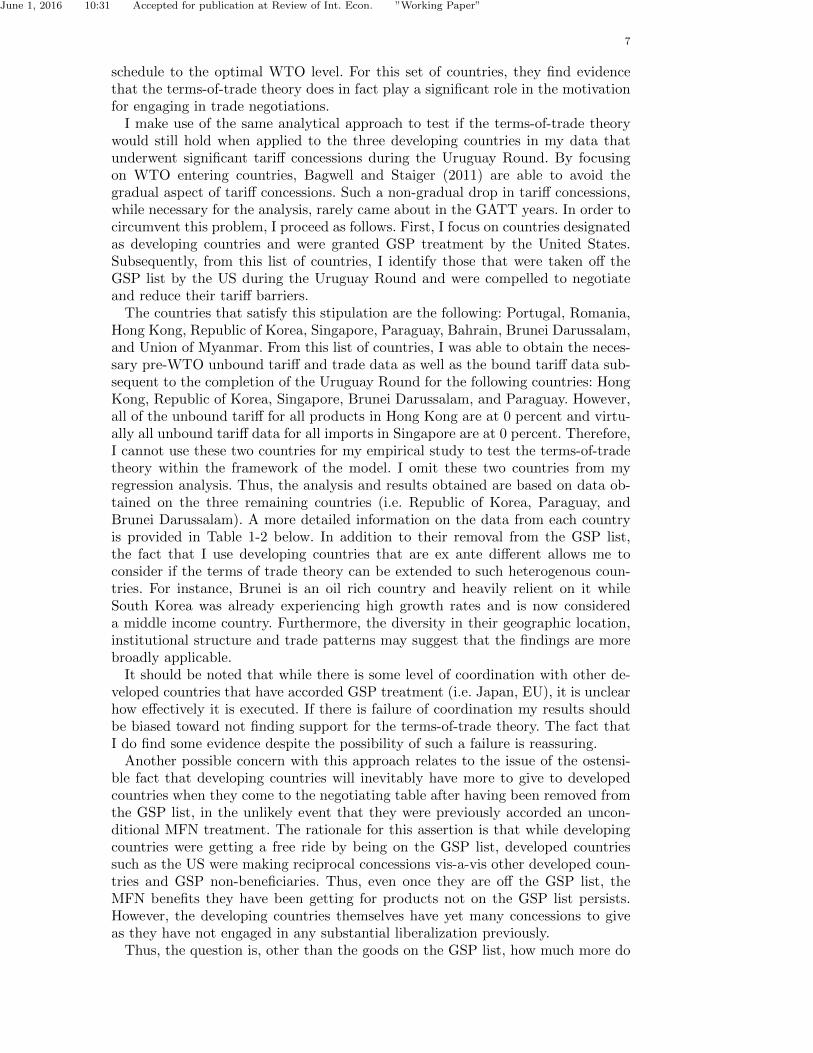
In Table 1, I report the list of countries in my sample, the year for which Ihave their import value data as well as their bound and unbound tariff data. Theunbound tariff data is generated on the WITS website using the TRAINS Databaseas the source. The bound tariff data and import value data are generated on theWTO website using the Integrated Data Base (IDB). Import value are in millionsof US dollars and tariffs are ad valorem. Table 1 shows (1) that the unbound tariffobservations are from years that precede the bound tariff observations and (2) thatthe largest gap in years between the unbound tariff and bound tariff for any of thecountries is no more than four years. While the former is a necessary condition forthe model to work, the latter is important in that the short time duration betweenthe two sets of observations allows for more precise estimations as time dependenttrends in trade are less likely to influence the results.

Table 1. Countries in the Sample

Country Year of Import Year of Unbound Tariff Year of Bound Tariff

Brunei 1992 1992 1996

Korea 1992 1992 1996

Paraguay 1994 1994 1996

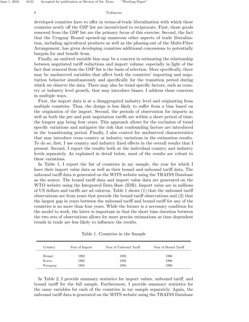
In Table 2, I provide summary statistics for import values, unbound tariff, andbound tariff for the full sample. Furthermore, I provide summary statistics forthe same variables for each of the countries in my sample separately. Again, theunbound tariff data is generated on the WITS website using the TRAINS Database


9

as the source. The bound tariff data and the import value data are generated onthe WTO website using the Integrated Data Base (IDB).

Table 2. Summary Statistics for Imports, Unbound Tariffs, and Bound Tariffs

Sample Variable Mean SD Min Max Observations

All Imports 8.04 106.61 0.00 9548.44 10636Unbound Tariff 7.34 9.54 0 602.67 14961Bound Tariff 35.07 21.87 1 92 13660

Brunei Imports 0.68 3.79 0.00 112.06 2157Unbound Tariff 2.42 11.01 0 602.67 5001Bound Tariff 28.19 13.08 1 69 4559

Korea Imports 17.15 158.82 0.00 9548.436 4761Unbound Tariff 11.75 6.95 0 50 4942Bound Tariff 30.78 31.29 2 92 4543

Paraguay Imports 0.65 3.94 0.00 137.63 3718Unbound Tariff 7.90 7.69 0 32 5018Bound Tariff 46.23 9.79 4 49 4558

5. Results

As noted before, the terms-of-trade theory suggests that countries negotiate andenter into trade agreements in order to mitigate a terms-of-trade prisoner’s dilemmaby reciprocally reducing trade barriers. Accordingly, the model predicts that, ceterisparibus, the negotiation based reduction in the tariff level from the best responseunbound tariff is higher when the trade value on that product is higher. Thus,the bound tariff on any given product to which a negotiating country agrees isexpected to be decreasing relative to the noncooperative tariff level as the importvalue of the product increases.

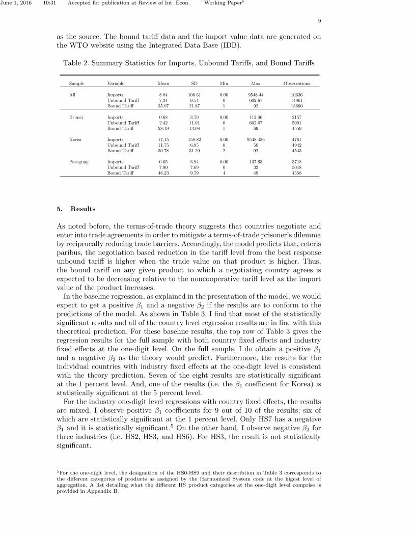
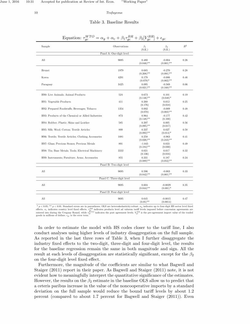
In the baseline regression, as explained in the presentation of the model, we wouldexpect to get a positive β1 and a negative β2 if the results are to conform to thepredictions of the model. As shown in Table 3, I find that most of the statisticallysignificant results and all of the country level regression results are in line with thistheoretical prediction. For these baseline results, the top row of Table 3 gives theregression results for the full sample with both country fixed effects and industryfixed effects at the one-digit level. On the full sample, I do obtain a positive β1

and a negative β2 as the theory would predict. Furthermore, the results for theindividual countries with industry fixed effects at the one-digit level is consistentwith the theory prediction. Seven of the eight results are statistically significantat the 1 percent level. And, one of the results (i.e. the β1 coefficient for Korea) isstatistically significant at the 5 percent level.

For the industry one-digit level regressions with country fixed effects, the resultsare mixed. I observe positive β1 coefficients for 9 out of 10 of the results; six ofwhich are statistically significant at the 1 percent level. Only HS7 has a negativeβ1 and it is statistically significant.5 On the other hand, I observe negative β2 forthree industries (i.e. HS2, HS3, and HS6). For HS3, the result is not statisticallysignificant.

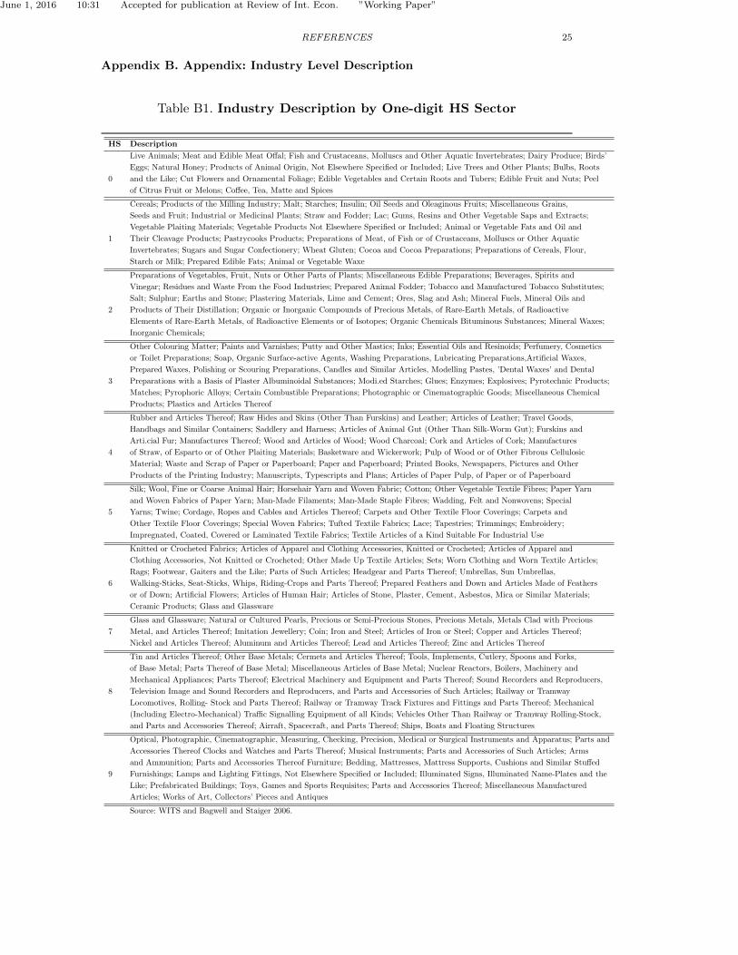
5For the one-digit level, the designation of the HS0-HS9 and their describtion in Table 3 corresponds tothe different categories of products as assigned by the Harmonized System code at the higest level ofaggregation. A list detailing what the different HS product categories at the one-digit level comprise isprovided in Appendix B.


10 Tesfayesus

Table 3. Baseline Results

Equation: τWTOgc = αg + αc + β1τ

BRgc + β2[V BR

gc ] + εgc

Sample Observations β1 β2 R2

(S.E.) (S.E.)

Panel A: One-digit level

All 9695 0.480 -0.004 0.26(0.046)** (0.001)**

Brunei 1979 0.685 -0.270 0.28(0.208)** (0.091)**

Korea 4291 0.178 -0.006 0.46(0.079)* (0.002)**

Paraguay 3425 0.095 -0.569 0.06(0.021)** (0.160)**

HS0: Live Animals; Animal Products 524 0.673 0.101 0.19(0.146)** (0.048)*

HS1: Vegetable Products 411 0.268 0.012 0.25(0.176) (0.018)

HS2: Prepared Foodstuffs; Beverages; Tobacco 1354 0.002 -0.009 0.48(0.070) (0.002)**

HS3: Products of the Chemical or Allied Industries 873 0.964 -0.177 0.42(0.148)** (0.100)

HS4: Rubber; Plastic; Skins and Leather 585 0.397 0.005 0.56(0.095)** (0.017)

HS5: Silk; Wool; Cotton; Textile Articles 899 0.337 0.027 0.58(0.092)** (0.014)*

HS6: Textile; Textile Articles; Clothing Accessories 1081 0.258 -0.963 0.41(0.026)** (0.243)**

HS7: Glass; Precious Stones; Precious Metals 891 -1.045 0.023 0.49(0.184)** (0.030)

HS8: Tin; Base Metals; Tools; Electrical Machinery 2222 0.021 0.017 0.32(0.136) (0.016)

HS9: Instruments; Furniture; Arms; Accessories 855 0.331 0.187 0.24(0.089)** (0.052)**

Panel B: Two-digit level

All 9695 0.596 -0.003 0.33(0.042)** (0.001)**

Panel C: Three-digit level

All 9695 0.604 -0.0029 0.35(0.044)** (0.001)*

Panel D: Four-digit level

All 9695 0.645 -0.0015 0.47(0.05)** (0.0014)

* p < 0.05; ** p < 0.01. Standard errors are in parentheses. OLS are heteroskedasticity-robust. αg indicates up to four-digit HS sector level fixedeffects. αc indicates country level fixed effects. τBR

gc indicates products level ad valorem tariff levels imposed before concession agreements are

entered into during the Uruguay Round, while τWTOgc indicates the post agreement levels. V BR

gc is the pre-agreement import value of the tradedgoods in millions of dollars. εgc is the error term.

In order to estimate the model with HS codes closer to the tariff line, I alsoconduct analyses using higher levels of industry disaggregation on the full sample.As reported in the last three rows of Table 3, when I further disaggregate theindustry fixed effects to the two-digit, three-digit and four-digit level, the resultsfor the baseline regression remain the same in both magnitude and sign. All theresult at each levels of disaggregation are statistically significant, except for the β2

on the four-digit level fixed effect.Furthermore, the magnitude of the coefficients are similar to what Bagwell and

Staiger (2011) report in their paper. As Bagwell and Staiger (2011) note, it is notevident how to meaningfully interpret the quantitative significance of the estimates.However, the results on the β2 estimate in the baseline OLS allow us to predict thata ceteris paribus increase in the value of the noncooperative imports by a standarddeviation on the full sample would reduce the bound tariff levels by about 1.2percent (compared to about 1.7 percent for Bagwell and Staiger (2011)). Even


11

when the analysis is extended to the Uruguay years focusing on three developingcountries analyzed here with country and industry fixed effects at various levelsof disaggregation, the results that I obtain are in line with the predictions of theterms-of-trade prisoner’s dilemma theory.6

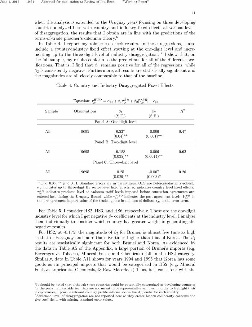
In Table 4, I report my robustness check results. In these regressions, I alsoinclude a country-industry fixed effect starting at the one-digit level and incre-menting up to the three-digit level of industry disaggregation. 7 I show that, onthe full sample, my results conform to the predictions for all of the different spec-ifications. That is, I find that β1 remains positive for all of the regressions, whileβ2 is consistently negative. Furthermore, all results are statistically significant andthe magnitudes are all closely comparable to that of the baseline.

Table 4. Country and Industry Disaggregated Fixed Effects

Equation: τWTOgc = αgc + β1τ

BRgc + β2[V BR

gc ] + εgc


(S.E.) (S.E.)

Panel A: One-digit level

All 9695 0.227 -0.006 0.47(0.04)** (0.001)**

Panel B: Two-digit level

All 9695 0.188 -0.006 0.62(0.035)** (0.0014)**

Panel C: Three-digit level

All 9695 0.25 -0.007 0.26(0.029)** (0.003)*

* p < 0.05; ** p < 0.01. Standard errors are in parentheses. OLS are heteroskedasticity-robust.αg indicates up to three-digit HS sector level fixed effects. αc indicates country level fixed effects.τBRgc indicates products level ad valorem tariff levels imposed before concession agreements are

entered into during the Uruguay Round, while τWTOgc indicates the post agreement levels. V BR

gc isthe pre-agreement import value of the traded goods in millions of dollars. εgc is the error term.

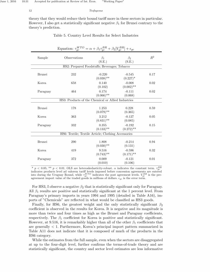
For Table 5, I consider HS2, HS3, and HS6, respectively. These are the one-digitindustry level for which I get negative β2 coefficients at the industry level. I analyzethem individually to consider which country has greater weight in generating thenegative results.

For HS2, at -0.175, the magnitude of β2 for Brunei, is almost five time as highas that of Paraguay and more than five times higher than that of Korea. The β2

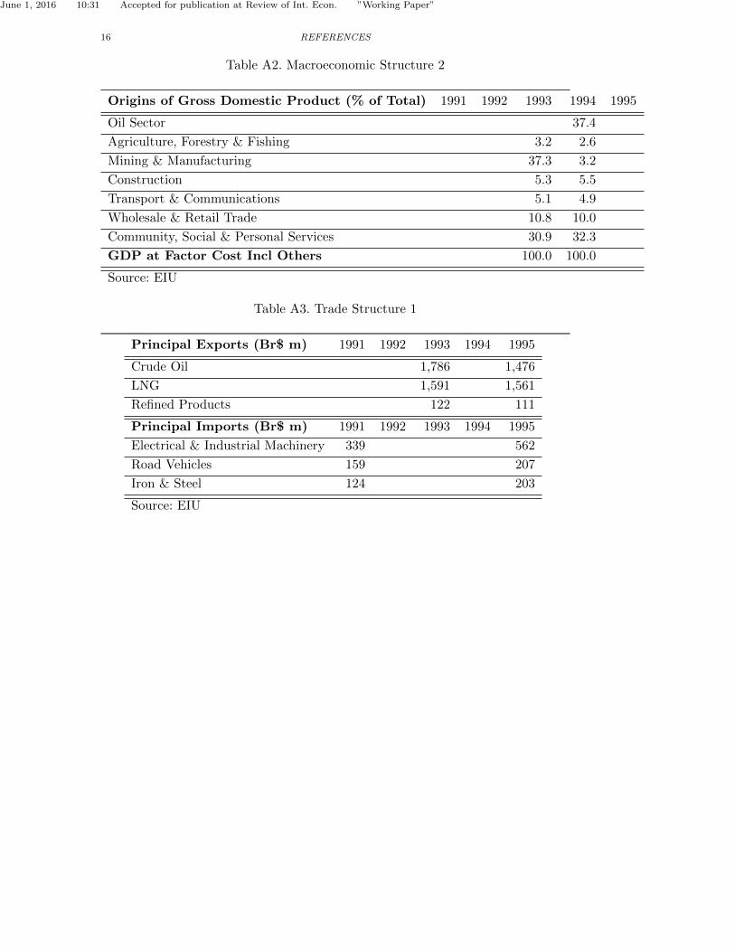
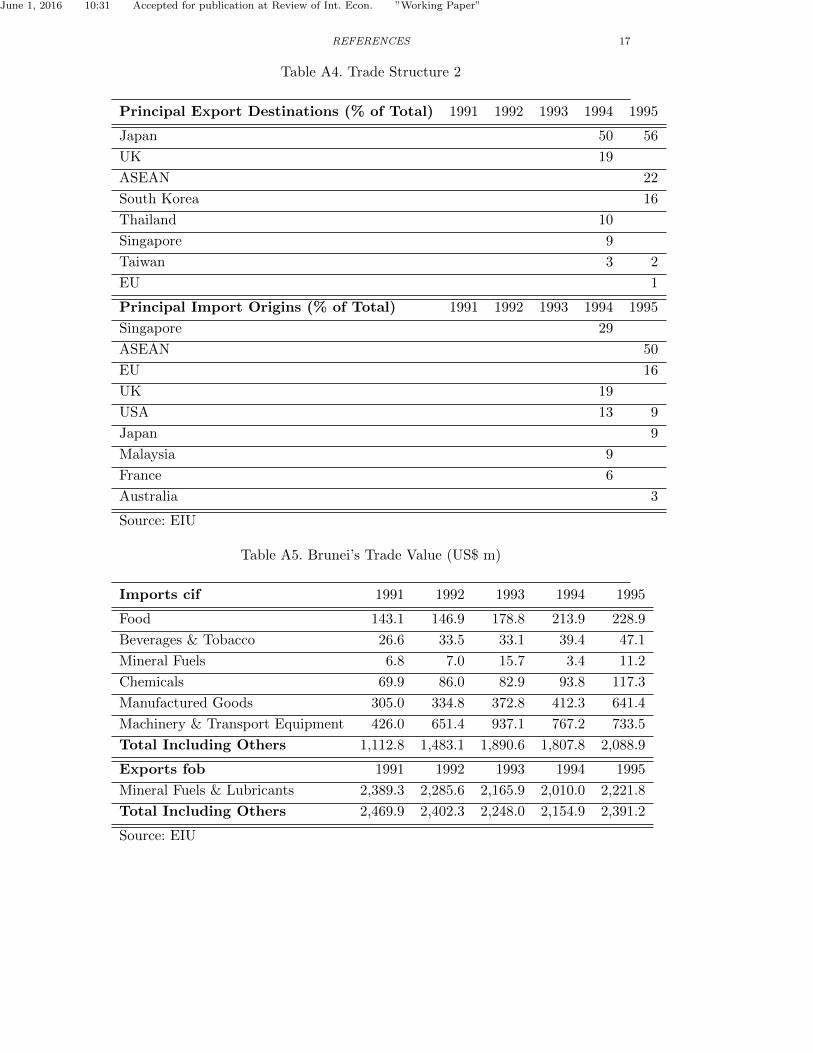
results are statistically significant for both Brunei and Korea. As evidenced bythe data in Table A5 of the Appendix, a large portion of Brunei’s imports (e.g.Beverages & Tobacco, Mineral Fuels, and Chemicals) fall in the HS2 category.Similarly, data in Table A11 shows for years 1994 and 1995 that Korea has somegoods as its principal imports that would be categorized in HS2 (e.g. MineralFuels & Lubricants, Chemicals, & Raw Materials.) Thus, it is consistent with the

6It should be noted that although these countries could be potentially categorized as developing countriesfor the years I am considering, they are not meant to be representative samples. In order to highlight theiridiosyncrasies, I provide relevant country profile information in the Appendix for each country.7Additional level of disaggregation are not reported here as they create hidden collinearity concerns andgive coefficients with missing standard error values.


12 Tesfayesus

theory that they would reduce their bound tariff more in these sectors in particular.However, I also get a statistically significant negative β1 for Brunei contrary to thetheory’s prediction.

Table 5. Country Level Results for Select Industries

Equation: τWTOgc = α+ β1τ

BRgc + β2[V BR

gc ] + εgc


(S.E.) (S.E.)

HS2: Prepared Foodstuffs; Beverages; Tobacco

Brunei 232 -0.220 -0.545 0.17(0.038)** (0.227)*

Korea 658 0.140 -0.008 0.02(0.102) (0.002)**

Paraguay 464 0.174 -0.111 0.02(0.066)** (0.068)

HS3: Products of the Chemical or Allied Industries

Brunei 178 1.253 0.228 0.59(0.079)** (0.365)

Korea 363 3.212 -0.127 0.05(0.831)** (0.085)

Paraguay 332 0.355 -0.192 0.15(0.133)** (0.272)**

HS6: Textile; Textile Article; Clothing Accessories

Brunei 290 1.808 -0.214 0.94(0.030)** (0.131)

Korea 419 9.516 -0.596 0.32(0.743)** (0.171)**

Paraguay 372 0.009 -0.121 0.01(0.010) (0.106)

* p < 0.05; ** p < 0.01. OLS are heteroskedasticity-robust. α indicates the constant term. τBRgc

indicates products level ad valorem tariff levels imposed before concession agreements are enteredinto during the Uruguay Round, while τWTO

gc indicates the post agreement levels. V BRgc is the pre-

agreement import value of the traded goods in millions of dollars. εgc is the error term.

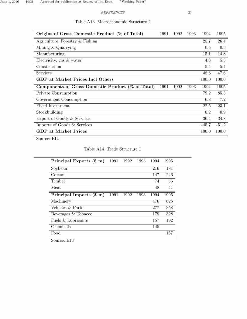
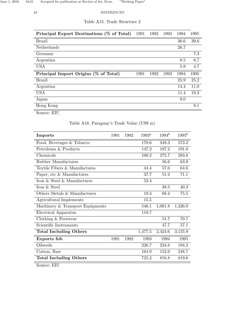
For HS3, I observe a negative β2 that is statistically significant only for Paraguay.All β1 results are positive and statistically significant at the 1 percent level. FromParaguay’s primary imports in years 1994 and 1995 (detailed in Table A16), im-ports of ”Chemicals” are reflected in what would be classified as HS3 goods.

Finally, for HS6, the greatest weight and the only statistically significant β2

coefficient is observed in the results for Korea. It is negative and its magnitude ismore than twice and four times as high as the Brunei and Paraguay coefficients,respectively. The β1 coefficient for Korea is positive and statistically significant.However, at 9.516, it is remarkably higher than all of the other β1 coefficients thatare generally < 1. Furthermore, Korea’s principal import pattern summarized inTable A11 does not indicate that it is composed of much of the products in theHS6 category.

While the estimates from the full sample, even when the sectors are disaggregatedat up to the four-digit level, further confirms the terms-of-trade theory and arestatistically significant, the country and sector level estimates are less informative


13

and not clearly accounted for by the theory. However, the finding of such preciseresults substantiating the terms-of-trade theory at up to the four-digit level ofdisaggregation even using the full sample is certainly noteworthy.

6. Conclusion

In this study, I present and explain frameworks to test the validity of the terms-of-trade based theoretical explanation for why countries enter into agreements usingthe GATT/WTO as a forum for negotiations. Then, I test the relevance of thistheory using a structural model that predicts that negotiated tariff concessions arelarger for products with higher total import value.

Based on my results using Uruguay Round trade and tariff data for three transi-tioning economies removed from the US GSP list, I find that my estimates supportthe predictions of the terms-of-trade theory relationship. This holds true even whenI disaggregate the industry fixed effects up to the four-digit level or when I applya country-industry fixed effect in the baseline estimation. The results at the indi-vidual country level are also in line with the predictions, although the results atthe individual industry level analyses are less conclusive.


14 REFERENCES

References

Antras, P., Staiger, R.W., 2012. Offshoring and the Role of Trade Agreements. TheAmerican Economic Review 102(7), 3140-83

Bagwell, K., Staiger, R.W., 1999. An Economic Theory of the GATT. The Amer-ican Economic Review 89(1), 215-248.

Bagwell, K., Staiger, R.W., 2002. The Economics of The World Trading System.The MIT Press.

Bagwell, K., Staiger, R.W., 2006. What Do Trade Negotiators Negotiate About?Empirical Evidence from the World Trade Organization. NBER Working Pa-per 12727.

Bagwell, K., Staiger, R.W., 2011. What Do Trade Negotiators Negotiate About?Empirical Evidence from the World Trade Organization. The American Eco-nomic Review 101, 1238-1273.

Baldwin, R., Robert-Nicoud, F., 2000. Free Trade Agreements with Delocation.Canadian Journal of Economics 33(3), 766-786.

Grossman, G.M., Helpman, E., 1995a. Trade wars and trade talks. Journal of Po-litical Economy 103, 675-708.

Johnson, H.G., 1953-54. Optimum tariffs and retaliation. Review of Economic Stud-ies 21, 142-153.

Krugman, P.R., 1980. Scale Economies, Product Differentiation, and the Patternof Trade. American Economic Review 70(5), 950-959.

Ludema, R.D., Mayda, A.M., 2013. Do Terms-of-trade Effects Matter for TradeAgreements? Theory and Evidence from WTO Countries. Quarterly Journalof Economics 128(2), 1837-1893.

Maggi, G., Rodriguez-Clare, A., 2007. A Political-Economy Theory of Trade Agree-ments. American Economic Review 97(4), 1374-1406.

Mayer, W., 1981. Theoretical Considerations on Negotiated Tariff Adjustments.Oxford Economic Papers 33(1), 135-153.

Ossa, R., 2011. A New Trade Theory of GATT/WTO Negotiations. Journal ofPolitical Economy 119(1), 122-152.

Venables, A., 1987. Trade and Trade Policy with Differentiated Products: AChamberlinian-Ricardian Model. The Economic Journal 97(387), 700-717.


REFERENCES 15

Appendix A. Appendix: Country Level Description

Figure A1.: Brunei

Source: www.mapsopensource.com

Table A1. Macroeconomic Structure 1

Economic Indicators 1991 1992 1993 1994 1995

Real GDP Growth 1.5a -1.1 0.5 1.8 2.0b

Consumer Price Inflation 1.6 1.3 4.3 2.4 6.0a

Population ’000 263a 267.8 276.3 284.5 292.0a

Exports fob US$ bn 2.5a 2.4 2.3 2.2 2.4

Imports fob US$ bn 1.2a 1.2 1.2 1.7 1.98

Exchange rate (av) Br$:US$ 1.73 1.63 1.62 1.53 1.42

Source: EIUa EIU estimates.b Official estimate.


16 REFERENCES


Origins of Gross Domestic Product (% of Total) 1991 1992 1993 1994 1995

Oil Sector 37.4

Agriculture, Forestry & Fishing 3.2 2.6

Mining & Manufacturing 37.3 3.2

Construction 5.3 5.5

Transport & Communications 5.1 4.9

Wholesale & Retail Trade 10.8 10.0

Community, Social & Personal Services 30.9 32.3

GDP at Factor Cost Incl Others 100.0 100.0

Source: EIU

Table A3. Trade Structure 1

Principal Exports (Br$ m) 1991 1992 1993 1994 1995

Crude Oil 1,786 1,476

LNG 1,591 1,561

Refined Products 122 111

Principal Imports (Br$ m) 1991 1992 1993 1994 1995

Electrical & Industrial Machinery 339 562

Road Vehicles 159 207

Iron & Steel 124 203

Source: EIU


REFERENCES 17


Principal Export Destinations (% of Total) 1991 1992 1993 1994 1995

Japan 50 56

UK 19

ASEAN 22

South Korea 16

Thailand 10

Singapore 9

Taiwan 3 2

EU 1

Principal Import Origins (% of Total) 1991 1992 1993 1994 1995

Singapore 29

ASEAN 50

EU 16

UK 19

USA 13 9

Japan 9

Malaysia 9

France 6

Australia 3

Source: EIU

Table A5. Brunei’s Trade Value (US$ m)

Imports cif 1991 1992 1993 1994 1995

Food 143.1 146.9 178.8 213.9 228.9

Beverages & Tobacco 26.6 33.5 33.1 39.4 47.1

Mineral Fuels 6.8 7.0 15.7 3.4 11.2

Chemicals 69.9 86.0 82.9 93.8 117.3

Manufactured Goods 305.0 334.8 372.8 412.3 641.4

Machinery & Transport Equipment 426.0 651.4 937.1 767.2 733.5

Total Including Others 1,112.8 1,483.1 1,890.6 1,807.8 2,088.9

Exports fob 1991 1992 1993 1994 1995

Mineral Fuels & Lubricants 2,389.3 2,285.6 2,165.9 2,010.0 2,221.8

Total Including Others 2,469.9 2,402.3 2,248.0 2,154.9 2,391.2

Source: EIU


18 REFERENCES

Table A6. Brunei’s Trade Direction (US$ m)

Total Export fob 1991 1992 1993a 1994a 1995a

Japan 1,543 1,287 1,079 1,220

UK 414 416 182

South Korea 254

Thailand 203 206 166 263

Singapore 165 196 189 203

Taiwan 61 56 46

Philippines 96

Total Including Others 2,466 2,362 2,084 2,329

Total Imports cif 1991 1992 1993a 1994a 1995a

Singapore 245 698 897 1,612

UK 78 495 595 444

Japan 175

USA 152 526 414 209

Malaysia 107 207 287 358

Total Including Others 1,111 2,600 3,124 3,490

Source: EIUa DOTs estimate.


REFERENCES 19

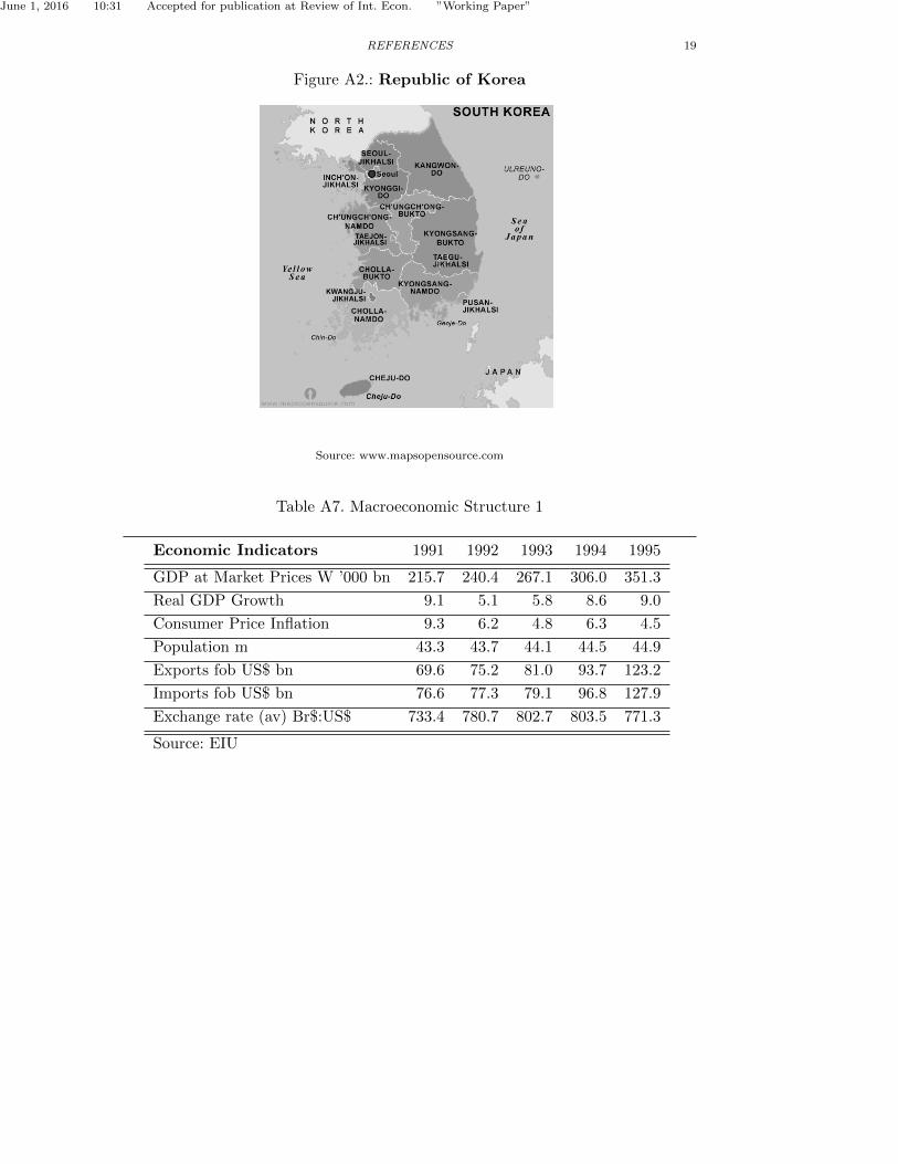
Figure A2.: Republic of Korea




GDP at Market Prices W ’000 bn 215.7 240.4 267.1 306.0 351.3

Real GDP Growth 9.1 5.1 5.8 8.6 9.0

Consumer Price Inflation 9.3 6.2 4.8 6.3 4.5

Population m 43.3 43.7 44.1 44.5 44.9

Exports fob US$ bn 69.6 75.2 81.0 93.7 123.2

Imports fob US$ bn 76.6 77.3 79.1 96.8 127.9

Exchange rate (av) Br$:US$ 733.4 780.7 802.7 803.5 771.3

Source: EIU


20 REFERENCES




Mining & Quarrying 0.3 0.3

Manufacturing 26.9 29.9

Electricity, gas & water 2.3 2.4


Trade, Restaurant, & Hotels 11.7 12.5

Transport, Storage, & Communications 7.4 7.9

Fiancial & Business Services 17.1 17.2

Government Services 7.9 5.8

GDP at Market Prices Incl Others 100.0 100.0

Components of Gross Domestic Product (% of Total) 1991 1992 1993 1994 1995

Private Consumption 53.8 52.9

Government Concumption 10.6 10.4

Fixed Capital Formation 35.9 36.6

Change in Stocks 0.1 0.5

Export of Goods & Services 30.1 33.2

Imports of Goods & Services -30.9 -34.2

Statistical Discrepancy 0.4 0.6

GDP at Market Prices 100.0 100.0

Source: EIU


Principal Exports ($ m) 1991 1992 1993 1994 1995

Transistors, Semiconductors etc 11,848 19,373

Textiles & Fabrics 7,839 10,065

Passenger Cars 7,242

Ships & Floating Structures 4,945 5,533

Clothing & Accessories 5,652 4,958

Total Incl Others 96,013 125,058

Principal Imports ($ m) 1991 1992 1993 1994 1995

Machinery & Transport Equipment 37,408 49,437

Mineral Fuels & Lubricants 15,406 19,013

Chemicals 9,762 13,156

Raw Materials 9,405 11,713

Food & Live Animals 4,761 5,926

Total Incl Others 102,349 135,119

Source: EIU


REFERENCES 21



USA 21.4 19.3

Japan 14.1 13.6

Hong Kong 8.3 8.5

China 6.5 7.6

Germany 4.5 4.8


Japan 24.8 24.1

USA 21.1 22.5

China 5.3 5.7

Germany 5.0 4.9

Saudi Arabia 3.7 4.0

Source: EIU

Table A11. Korea’s Trade Value (US$ m)

Imports of Selected Commodities 1991 1992 1993 1994 1995

Machinery & Transport Equipment 28,417 37,408 49,437

Measuring & Controlling Instruments 2,049 2,664 3,607

Mineral Fuels, Lubricants etc 15,053 15,415 19,013

Chemicals 8,235 9,763 13,156

Inedible Raw Material 8,870 9,405 11,713

Food & Live Animals 4,002 4,761 5,926

Total Including Others 83,800 102,348 135,119

Exports of Selected Commodities 1991 1992 1993 1994 1995

Total 82,236 96,013 125,058

Source: EIU


22 REFERENCES

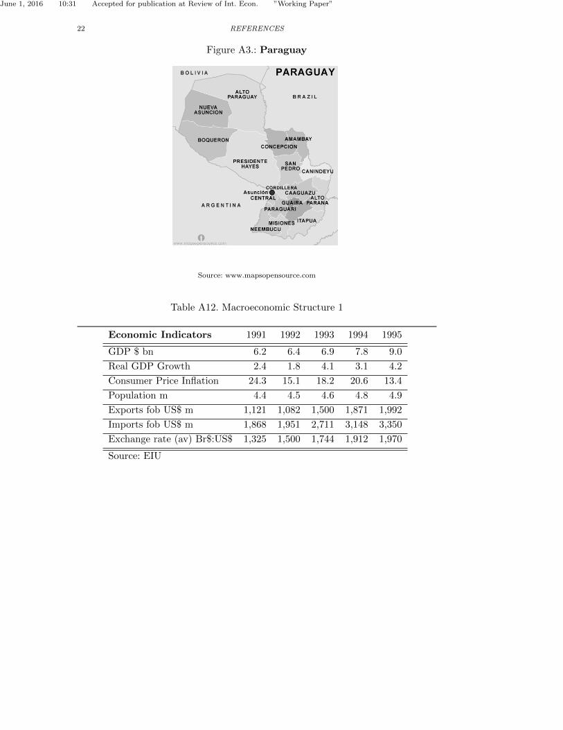
Figure A3.: Paraguay




GDP $ bn 6.2 6.4 6.9 7.8 9.0

Real GDP Growth 2.4 1.8 4.1 3.1 4.2

Consumer Price Inflation 24.3 15.1 18.2 20.6 13.4

Population m 4.4 4.5 4.6 4.8 4.9

Exports fob US$ m 1,121 1,082 1,500 1,871 1,992

Imports fob US$ m 1,868 1,951 2,711 3,148 3,350

Exchange rate (av) Br$:US$ 1,325 1,500 1,744 1,912 1,970

Source: EIU


REFERENCES 23




Mining & Quarrying 0.5 0.5

Manufacturing 15.1 14.8

Electricity, gas & water 4.8 5.3


Services 48.6 47.6

GDP at Market Prices Incl Others 100.0 100.0

Components of Gross Domestic Product (% of Total) 1991 1992 1993 1994 1995

Private Consumption 79.2 85.3

Government Concumption 6.8 7.2

Fixed Investment 22.5 23.1

Stockbuilding 0.2 0.9

Export of Goods & Services 36.4 34.8

Imports of Goods & Services -45.7 -51.2

GDP at Market Prices 100.0 100.0

Source: EIU


Principal Exports ($ m) 1991 1992 1993 1994 1995

Soybean 216 181

Cotton 147 246

Timber 74 56

Meat 48 41

Principal Imports ($ m) 1991 1992 1993 1994 1995

Machinery 476 626

Vehicles & Parts 277 358

Beverages & Tobacco 179 328

Fuels & Lubricants 157 192

Chemicals 145

Food 157

Source: EIU


24 REFERENCES



Brazil 36.6 39.6

Netherlands 26.7

Germany 7.3

Argentina 8.5 6.7

USA 5.9 4.7


Brazil 25.9 25.2

Argentina 14.4 11.0

USA 11.4 19.3

Japan 9.0

Hong Kong 8.1

Source: EIU

Table A16. Paraguay’s Trade Value (US$ m)

Imports 1991 1992 1993a 1994b 1995b

Food, Beverages & Tobacco 178.6 348.3 573.2

Petroleum & Products 147.2 187.2 191.0

Chemicals 100.2 275.7 283.8

Rubber Manufactures 56.6 63.9

Textile Fibers & Manufactures 44.4 57.6 64.6

Paper, etc & Manufactures 37.7 51.2 71.1

Iron & Steel & Manufactures 53.4

Iron & Steel 38.5 40.3

Others Metals & Manufactures 19.4 68.4 75.5

Agricultural Implements 15.5

Machinery & Transport Equipments 546.1 1,001.8 1,326.0

Electrical Apparatus 119.7

Clothing & Footwear 51.7 70.7

Scientific Instruments 47.7 57.1

Total Including Others 1,477.5 2,424.6 3,135.9

Exports fob 1991 1992 1993 1994 1995

Oilseeds 226.7 224.8 194.2

Cotton, Raw 164.9 153.9 248.7

Total Including Others 725.2 816.8 819.6

Source: EIU


REFERENCES 25

Appendix B. Appendix: Industry Level Description

Table B1. Industry Description by One-digit HS Sector

HS Description

Live Animals; Meat and Edible Meat Offal; Fish and Crustaceans, Molluscs and Other Aquatic Invertebrates; Dairy Produce; Birds’

Eggs; Natural Honey; Products of Animal Origin, Not Elsewhere Specified or Included; Live Trees and Other Plants; Bulbs, Roots

0 and the Like; Cut Flowers and Ornamental Foliage; Edible Vegetables and Certain Roots and Tubers; Edible Fruit and Nuts; Peel

of Citrus Fruit or Melons; Coffee, Tea, Matte and Spices

Cereals; Products of the Milling Industry; Malt; Starches; Insulin; Oil Seeds and Oleaginous Fruits; Miscellaneous Grains,

Seeds and Fruit; Industrial or Medicinal Plants; Straw and Fodder; Lac; Gums, Resins and Other Vegetable Saps and Extracts;

Vegetable Plaiting Materials; Vegetable Products Not Elsewhere Specified or Included; Animal or Vegetable Fats and Oil and

1 Their Cleavage Products; Pastrycooks Products; Preparations of Meat, of Fish or of Crustaceans, Molluscs or Other Aquatic

Invertebrates; Sugars and Sugar Confectionery; Wheat Gluten; Cocoa and Cocoa Preparations; Preparations of Cereals, Flour,

Starch or Milk; Prepared Edible Fats; Animal or Vegetable Waxe

Preparations of Vegetables, Fruit, Nuts or Other Parts of Plants; Miscellaneous Edible Preparations; Beverages, Spirits and

Vinegar; Residues and Waste From the Food Industries; Prepared Animal Fodder; Tobacco and Manufactured Tobacco Substitutes;

Salt; Sulphur; Earths and Stone; Plastering Materials, Lime and Cement; Ores, Slag and Ash; Mineral Fuels, Mineral Oils and

2 Products of Their Distillation; Organic or Inorganic Compounds of Precious Metals, of Rare-Earth Metals, of Radioactive

Elements of Rare-Earth Metals, of Radioactive Elements or of Isotopes; Organic Chemicals Bituminous Substances; Mineral Waxes;

Inorganic Chemicals;

Other Colouring Matter; Paints and Varnishes; Putty and Other Mastics; Inks; Essential Oils and Resinoids; Perfumery, Cosmetics

or Toilet Preparations; Soap, Organic Surface-active Agents, Washing Preparations, Lubricating Preparations,Artificial Waxes,

Prepared Waxes, Polishing or Scouring Preparations, Candles and Similar Articles, Modelling Pastes, ’Dental Waxes’ and Dental

3 Preparations with a Basis of Plaster Albuminoidal Substances; Modi.ed Starches; Glues; Enzymes; Explosives; Pyrotechnic Products;

Matches; Pyrophoric Alloys; Certain Combustible Preparations; Photographic or Cinematographic Goods; Miscellaneous Chemical

Products; Plastics and Articles Thereof

Rubber and Articles Thereof; Raw Hides and Skins (Other Than Furskins) and Leather; Articles of Leather; Travel Goods,

Handbags and Similar Containers; Saddlery and Harness; Articles of Animal Gut (Other Than Silk-Worm Gut); Furskins and

Arti.cial Fur; Manufactures Thereof; Wood and Articles of Wood; Wood Charcoal; Cork and Articles of Cork; Manufactures

4 of Straw, of Esparto or of Other Plaiting Materials; Basketware and Wickerwork; Pulp of Wood or of Other Fibrous Cellulosic

Material; Waste and Scrap of Paper or Paperboard; Paper and Paperboard; Printed Books, Newspapers, Pictures and Other

Products of the Printing Industry; Manuscripts, Typescripts and Plans; Articles of Paper Pulp, of Paper or of Paperboard

Silk; Wool, Fine or Coarse Animal Hair; Horsehair Yarn and Woven Fabric; Cotton; Other Vegetable Textile Fibres; Paper Yarn

and Woven Fabrics of Paper Yarn; Man-Made Filaments; Man-Made Staple Fibres; Wadding, Felt and Nonwovens; Special

5 Yarns; Twine; Cordage, Ropes and Cables and Articles Thereof; Carpets and Other Textile Floor Coverings; Carpets and

Other Textile Floor Coverings; Special Woven Fabrics; Tufted Textile Fabrics; Lace; Tapestries; Trimmings; Embroidery;

Impregnated, Coated, Covered or Laminated Textile Fabrics; Textile Articles of a Kind Suitable For Industrial Use

Knitted or Crocheted Fabrics; Articles of Apparel and Clothing Accessories, Knitted or Crocheted; Articles of Apparel and

Clothing Accessories, Not Knitted or Crocheted; Other Made Up Textile Articles; Sets; Worn Clothing and Worn Textile Articles;

Rags; Footwear, Gaiters and the Like; Parts of Such Articles; Headgear and Parts Thereof; Umbrellas, Sun Umbrellas,

6 Walking-Sticks, Seat-Sticks, Whips, Riding-Crops and Parts Thereof; Prepared Feathers and Down and Articles Made of Feathers

or of Down; Artificial Flowers; Articles of Human Hair; Articles of Stone, Plaster, Cement, Asbestos, Mica or Similar Materials;

Ceramic Products; Glass and Glassware

Glass and Glassware; Natural or Cultured Pearls, Precious or Semi-Precious Stones, Precious Metals, Metals Clad with Precious

7 Metal, and Articles Thereof; Imitation Jewellery; Coin; Iron and Steel; Articles of Iron or Steel; Copper and Articles Thereof;

Nickel and Articles Thereof; Aluminum and Articles Thereof; Lead and Articles Thereof; Zinc and Articles Thereof

Tin and Articles Thereof; Other Base Metals; Cermets and Articles Thereof; Tools, Implements, Cutlery, Spoons and Forks,

of Base Metal; Parts Thereof of Base Metal; Miscellaneous Articles of Base Metal; Nuclear Reactors, Boilers, Machinery and

Mechanical Appliances; Parts Thereof; Electrical Machinery and Equipment and Parts Thereof; Sound Recorders and Reproducers,

8 Television Image and Sound Recorders and Reproducers, and Parts and Accessories of Such Articles; Railway or Tramway

Locomotives, Rolling- Stock and Parts Thereof; Railway or Tramway Track Fixtures and Fittings and Parts Thereof; Mechanical

(Including Electro-Mechanical) Traffic Signalling Equipment of all Kinds; Vehicles Other Than Railway or Tramway Rolling-Stock,

and Parts and Accessories Thereof; Airraft, Spacecraft, and Parts Thereof; Ships, Boats and Floating Structures

Optical, Photographic, Cinematographic, Measuring, Checking, Precision, Medical or Surgical Instruments and Apparatus; Parts and

Accessories Thereof Clocks and Watches and Parts Thereof; Musical Instruments; Parts and Accessories of Such Articles; Arms

and Ammunition; Parts and Accessories Thereof Furniture; Bedding, Mattresses, Mattress Supports, Cushions and Similar Stuffed

9 Furnishings; Lamps and Lighting Fittings, Not Elsewhere Specified or Included; Illuminated Signs, Illuminated Name-Plates and the

Like; Prefabricated Buildings; Toys, Games and Sports Requisites; Parts and Accessories Thereof; Miscellaneous Manufactured

Articles; Works of Art, Collectors’ Pieces and Antiques

Source: WITS and Bagwell and Staiger 2006.

Documents

Liberalization Agreements in the GATT/WTO and the Terms-of-trade