Liar’s Loan?

Effects of Origination Channel and Information Falsification on Mortgage Delinquency1

Wei Jiang2 Ashlyn Aiko Nelson3 Edward Vytlacil4

This Draft: February 2010

                                                            1 The authors thank a major national mortgage bank for providing the data and assistance in data processing and the National Science Foundation (NSF Grant #SES-0851428) for financial support. Comments and suggestions from Vyacheslav Fos, Chris Mayer, Daniel Paravisini, Tomasz Piskorski, David Scharfstein, Amit Seru, Bob Van Order, and seminar/conference participants at Columbia, Georgia State, Kansas City Federal Reserve Bank, the NBER 2009 Summer Institute, the FDIC 2009 Mortgage Symposium, and the 2010 AEA have contributed to this draft. The authors also thank Erica Blom, Sunyoung Park, and Mike Tannenbaum for excellent research assistance. 2 Corresponding author. Columbia Business School, Finance and Economics Division, Tel: 212 854 9002, Email: wj2006@columbia.edu. 3 Indiana University, School of Public and Environmental Affairs, Tel: 812 855 5971, Email: ashlyn@indiana.edu. 4 Yale University, Department of Economics, Tel: 203 436 3994, Email: edward.vytlacil@yale.edu.

2  

Liar’s Loan?

Effects of Origination Channel and Information Falsification on Mortgage Delinquency

ABSTRACT

This paper presents a comprehensive analysis of mortgage delinquency using a unique

loan-level dataset from a major national mortgage bank from 2004 to 2008. Our analysis

highlights two major agency problems underlying the mortgage crisis: one between the

bank and mortgage brokers that results in lower quality broker-originated loans, and the

other between banks and borrowers that results in information falsification by borrowers

of low-documentation loans--known in the industry as “liars’ loans”--especially when

originated through a broker. While nearly all the difference in delinquency rates between

bank and broker channels can be attributed to observable loan and borrower

characteristics, most of the difference between full- and low-documentation types is due

to unobservable heterogeneity. Both differences are not fully compensated by the loan

pricing.

The recent crisis in the housing and mortgage debt market has drawn considerable attention from

regulators and market participants. A decade-long boom in the housing market and related financial

sectors was followed in 2007 by a market bust with falling house prices and a rapid increase in mortgage

defaults and foreclosures. The nationwide delinquency rate on subprime loans reached 39% by early

2009, more than seven times the level in 2005.5 Those caught in the crisis included large financial

institutions that experienced sharp expansion in, and profited from, their exposure to mortgage loans. The

crisis that started from the mortgage market quickly spread to other financial markets and throughout the

economy.

We use the experience of a major national mortgage bank to uncover the determinants of the

mortgage crisis and the evolution of the crisis at a micro level. The particular bank provides an ideal

context for the study by presenting a representative and yet amplified version of the boom-and-bust cycle

experienced by the national mortgage sector in the last decade. First, the bank was among the nation’s

top ten mortgage banks in 2006 and was one of the fastest growing players in the mortgage market,

specializing in low- and no-documentation loans (nicknamed “liars’ loans,” which constitute a large

portion of the Alt-A loans) while also providing full-documentation loans (about 30% of their total loan

                                                            5 Source of information: LPS Applied Analytics website: http://www.lpsvcs.com/NewsRoom/IndustryData/Pages/default.aspx . Delinquency is commonly defined as payment delinquency of 60 days or more, including foreclosure.

3  

originations). Second, the bank suffered one of the largest losses in the industry since the 2007 crisis.

Loans issued by the bank since the beginning of 2004 reached a cumulative delinquency rate of 28% by

early 2009; approximately half of these delinquent loans were in the state of short sale or foreclosure.

Finally, the borrowers and properties underlying the bank’s loans during our sample period have fair

representations in all 50 states. Therefore, lessons from this particular bank have general implications for

the national mortgage market.

Our proprietary data set represents the most detailed and disaggregated data set used so far in the

mortgage loan literature. Our data set consists of all 721,767 loans that the bank originated between

January 2004 and February 2008. We have all of the information that the bank collected at the time of

loan origination, as well as monthly performance data for each loan through January 2009. Our data set

includes not only information about the loan (pricing, loan product, and other contractual terms) and the

property (address, appraisal value, owner occupancy status, etc.), but also about the borrowers

demographic characteristics (race, age, gender, etc.) and economic conditions (income, cash reserves,

employment status, etc.). Finally, we are able to use the property address information to match about

three-quarters of the loans to community attributes such as demographics and business opportunities in

narrow localities.

Our sample is divided into four distinct subsamples by a two-way sorting. The first sorting

variable is the loan origination channel: whether a loan is originated directly by the bank or through a

third party originator (such as a mortgage broker or a correspondent; henceforth, we simply call this

category brokered loans). The second sorting variable is the loan documentation level: whether a loan is

originated with full documentation of borrowers’ economic conditions or with various reduced levels of

documentation (including no documentation). Throughout the paper we refer to the four subsamples (with

the initial letters capitalized) as: Bank/Full-Doc; Bank/Low-Doc; Broker/Full-Doc; Broker/Low-Doc.

The Bank (Broker) subsamples include both Bank/Full-Doc and Bank/Low-Doc (Broker/Full-Doc and

Broker/Low-Doc) subsamples, and the Full-Doc (Low-Doc) subsamples are defined analogously.

Our empirical analysis uncovers two types of agency problems in mortgage lending which

constitute the fundamental causes of high loan delinquency rates, and by extension, the mortgage crisis.

The first agency problem lies between the bank and its mortgage brokers. We find that loans in the

Broker subsamples have delinquency probabilities that are 10-14 percentage points (or more than 50%)

higher than the Bank subsamples, a manifestation of the misalignment of incentives for brokers who issue

loans on the bank’s behalf for commissions but do not bear the long-term consequences of low-quality

loans. A binary decomposition attributes three-quarters of the Bank-Broker delinquency gap to

differences in observable borrower characteristics, and the remaining quarter to differences due to

unobserved heterogeneity. Hence, the higher delinquency rates among brokered loans are explained

4  

largely by broker penetration of borrower pools that were of observably worse quality (according to credit

score, loan-to-value ratio, income, etc.) than the borrower pools penetrated by the bank.

Within each origination channel, the Low-Doc subsample exhibits worse performance than the

Full-Doc subsample, and the difference in delinquency is 5-8 percentage points. The same decomposition

method reveals that unobserved heterogeneity explains nearly 100% of this difference. In contrast to the

Broker channel, the Low-Doc channel does not necessarily compromise lending standards along the

observable metrics, but suffers from less careful verification of some reported information (such as

income and owner occupancy status) or less diligent screening of borrowers along hard-to-quantify

measures (such as other major expenditures). This relation highlights the second agency problem that lies

between the lender and the borrower, where the latter could hide or even falsify unfavorable information,

especially in the context of lax screening and verification procedures.

We provide evidence of borrower information falsification at both individual variable and

aggregate levels. First, we find that both the in-sample goodness-of-fit and the out-of-sample predictive

power of our delinquency prediction model are about 50% higher for the Full-Doc subsamples than for

the Low-Doc subsamples. These differences suggest that borrower information collected for low-

documentation loans is of lower quality, either in terms of inaccurately recorded data or intentionally

falsified information, thereby compromising the ability of such information to predict delinquency.

Second, certain variables--notably income--exhibit weak or even perverse relations to delinquency

probabilities among low-documentation loans. These weak or perverse relations are especially evident in

the Broker/Low-Doc subsample, where brokers both apply looser lending standards and are less diligent

in verifying borrower information. The most plausible explanation for this observed pattern is

information falsification. Through further analysis, we conservatively estimate that the median magnitude

of income exaggeration is about 20% among low-documentation borrowers.

Finally, we examine whether loan pricing adequately incorporated the higher delinquency risk of

broker-originated and low-documentation loans. Among fixed rate loans, we find that low documentation

loans do indeed command a higher interest rate premium of 29 basis points, but there is little evidence of

a rate premium for broker-originated loans. Among adjustable rate mortgages, we find that rates re-set at

the end of our sample period are actually 69-77 basis points lower for broker-originated loans. Moreover,

the higher delinquency rates among brokered and low-documentation loans remain statistically and

economically significant after controlling for interest rates. Thus, there is little evidence that the bank’s

interest rate scheme adequately priced for the different delinquency rates across loan types. In addition to

weakened incentives for screening due to high securitization rates during our sample period, this may also

be explained by a lack of evidence of delinquency differences across origination channels and

documentation types until the second half of our sample period (2006-2007).

5  

Our paper builds on a fast-growing literature on the mortgage crisis,6 and most closely relates to a

few recent empirical papers exploring the causes of the mortgage crisis using large sample micro-level

archival data. Mian and Sufi (2008) identify the effects of the increase in the supply of mortgage credit

on fueling the housing bubble between 2001 and 2005, and on the subsequent large increase in mortgage

defaults. Demyanyk and Van Hemert (2008) and Keys, Mukherjee, Seru, and Vig (2008) both use data

from LoanPerformance, a provider of performance data on securitized loans. Demyanyk and Van Hemert

(2008) focus on the deterioration in loan quality between 2001 and 2006, while Keys, et al. (2008) focus

on how securitization weakens the incentive of lenders to screen loan applicants. The commercial or

government agency loan databases mentioned above usually do not include borrower demographic

characteristics, detailed loan contractual terms, or location (address) information, and usually only include

securitized loans. Some earlier papers (e.g., Munnell, Tootell, Browne, and McEneaney (1996)) obtain

demographic information from government data sources, such as those reported for compliance with the

Home Mortgage Disclosure Act (HMDA). However, loan performance and detailed location information

are absent from these data sources, as are certain central economic variables such as the borrowers' credit

scores and the loan-to-value ratio.

The contribution of this paper can be summarized as follows. First, our unique dataset allows us

to present the most comprehensive and updated predictive model of delinquency in the literature. The

comprehensive list of predictors—including data on loan contract terms, property characteristics, and

borrower attributes—afford us a better understanding of the determinants of loan delinquency and loan

pricing. Because we observe all loan and borrower attributes collected by the bank at origination, we are

able to decompose delinquency differences into loan and borrower characteristics observed by the bank,

versus those attributable to unobserved heterogeneity. Such decomposition provides us an accurate

calibration of the information possessed by the bank, which is essential for the analyses of the moral

hazard and adverse selection problems in the loan market.

Second, the composition of loans in this data set better reflects the mix of borrowers and loan

products originated nationally both before and during the mortgage crisis. Unlike most prior studies

(including the papers cited above and earlier studies such as Deng, Quigley, and Van Order (2000) and

Alexander, Grimshaw, McQueen, and Slade (2002)), our sample includes both prime and subprime loans,

full-documentation and low-documentation loans, loans kept on the bank’s balance sheet and loans sold

to the secondary mortgage market. As such, we are able to obtain separate analyses for different loan

types partitioned by origination channel and documentation status, and to attribute delinquency and

pricing to loan types with minimal omitted variable bias (in terms of the bank’s information set).

                                                            6 An incomplete list includes Chomsisengphet and Pennington-Cross (2006), Dell’Ariccia, Igan, and Laeven (2008), Mayer, Pense, and Sherlund (2008), and Ben-David (2008).

6  

Moreover, with loan performance information updated to early 2009, we are able to capture the full effect

of the crisis on the mortgage market.

Finally, we examine the extent to which mortgage pricing reflected market participants

recognition of the default risk associated with broker-originated and low-documentation loans. Our

access to the full information set that the bank had regarding borrower characteristics allows us to conduct

this analysis with minimal risk of an omitted variable bias.

The rest of the paper is organized as follows. The next section provides a detailed data

description. Section II contains a comprehensive analysis of predictive models of loan delinquency.

Section III models borrowers’ choices of loan origination channel and documentation level, and

decomposes the cross-subsample differences in delinquency rates into two components: one reflecting

observable borrower characteristics or lending standards, and another reflecting unobservable borrower

heterogeneity. Section IV documents and quantifies borrower information falsification among low-

documentation loans. Section V discusses the extent to which mortgage interest rates reflected the

incentive conflicts presented in the analysis. Finally, Section VI concludes.

I. Data and Sample Overview

A. Data Sources and Description

As described in the prior section, our proprietary data set contains 721,767 loans funded by the

bank between January 2004 and February 2008. Our sample includes prime, Alt-A, and subprime

mortgages.

The data set contains all information obtained at loan origination, including the loan contract

terms, property data, and borrower financial and demographic data, as well as monthly performance data

updated through January 2009. Loan contract information includes the loan terms (such as loan amount,

loan-to-value (LTV) ratio, interest rate, and prepayment penalty), loan purpose (such as home purchase or

refinance), origination channel (broker versus bank-originated), and documentation requirements.

Property data used in our analysis includes the property address, whether the property will be

owner-occupied and used as a primary residence or used as an investment property/second home, and

home appraisal value. Borrower data includes protected class demographic variables collected under the

Home Mortgage Disclosure Act (HMDA) such as race, ethnicity, gender, and age, as well as all financial

and credit information collected at origination: income, cash reserves, expenditures, additional debts,

bankruptcy and/or foreclosure status at loan origination, credit score,7 employment status, employment

                                                            7 Fair Isaacs Co. developed the first nationwide, general purpose credit scoring model and released the eponymous FICO score in 1989. Since then, each of the three major credit-reporting bureaus--Equifax, Experian, and

7  

tenure (months in current job), self-employment status, and whether there are multiple borrowers (usually

used as a proxy for marital status).

Finally, we have monthly performance data for each loan through January 2009, including the

monthly unpaid balance and the loan delinquency status: whether the loan payments are current or

delinquent, the number of days delinquent, and whether the property is in a state of short sale or

foreclosure.

We are able to use the recorded property addresses to match approximately three-quarters of the

loans to community attributes such as demographics and business opportunities in narrow localities.

Using the ArcGIS geo-coding software and Decennial Census geographic boundary files, we match the

property addresses to their census tract, zip code, metropolitan statistical area (MSA), and county. The

geographic distribution (at the county level) of the properties in our sample is plotted in Figure 1; the

sample properties have fair representations in all 50 states, and their distribution is roughly proportional to

population density.

[Insert Figure 1 here]

We also obtain the following information at the census tract level from the Decennial Census and

the Bureau of Labor Statistics: population count, median age of the residents, percent of residents who are

black or Hispanic, and unemployment rate. In addition, we obtain zip-code level average household

income information from the Internal Revenue Service's Individual Master File system.

B. Sample Overview

During the sample period, the bank experienced substantial changes in the composition of its

loans and borrowers, as did the national mortgage market. Figure 2 reveals several salient patterns. First,

the bank experienced a rapid increase in loan production during the mortgage boom, followed by a sharp

decline during the housing bust; new loan originations increased from about 20,000 in the first half of

2004 to a peak of over 154,000 in the second half of 2006, followed by precipitous decline starting in the

second half of 2007.

[Insert Figure 2 here.]

Figure 2 also shows that the rapid expansion in loan production was driven almost exclusively by

increased loan originations through the broker channel, and expansion of low-documentation loans

through the broker channel in particular. Broker-originated loans represented 73% of all loan originations

                                                                                                                                                                                                TransUnion--have developed proprietary credit scoring models and jointly developed the VantageScore to compete with FICO. Most mortgage lenders use these scores as the primary measure of borrower credit risk. While there is some variation across the models used by the three credit bureaus--depending on the specific credit events reported to and/or collected by each bureau--the credit score used in this study is numerically comparable and analytically equivalent to the FICO score.

8  

in the first half of 2004, increasing to 94% by the second half of 2006; while broker low-doc loans

accounted for 39% of originations in early 2004, they comprised 75% of loan originations by late 2006.

Cumulative delinquency rates progressively and substantially increased over the time period in

our sample; at 18 months after origination, only 6.7% of loans originated in the first half of 2004 were

ever more than 60 days delinquent, as compared to 23.9% of loans originated in the second half of 2007.

Demyanyk and Van Hemert (2008) document a similarly deteriorating trend for subprime loans from

2001-2006 using the LoanPerformance database.

We define all of the variables used in this paper in Table 1 Panel A, and we report their mean,

median, and standard deviation values at a semi-annual frequency in Table 1 Panel B.

[Insert Table 1 here.]

The time trends in the key determinants of delinquency reflect changes in housing prices, the

loosening of lending standards during the boom period (2005 - 2006), and the subsequent tightening of

loan underwriting guidelines by the bank starting in 2007. Mean loan-to-value ratios (LTV, the ratio of

loan amount to the property’s appraised value) decreased from 69% in late 2004 to 65% in early 2007

before climbing to 77% in early 2008, mostly varying inversely with housing prices. Median borrower

credit score was 707 in early 2004, ranged from 689-694 in 2006 through early 2007, and subsequently

increased in 2007. Simultaneously, median reported income increased from $5,500 per month in early

2004 to $6,500 in late 2006, before trending downward. The growth in borrowers’ incomes through the

end of 2006 may result from the booming economy as well as from borrower income falsification on low-

documentation loans. Statistics on borrower job tenure exhibit a U-shape: median job tenure (a proxy for

job stability) decreased from 60 to 50 months at the peak of the boom, before bouncing back to 60 months

at the end of the sample period.

The housing boom welcomed many first-time homebuyers to the mortgage market. In early 2004,

only 7.6% of borrowers in the sample were first-time homebuyers, a figure that climbed to 18.1% by late

2006. As the housing market collapsed and lenders tightened standards, the percent of first-timers fell to

12.7% by the end of 2007. During the sample period, black and Hispanic borrowers gained a

significantly higher share of new loan originations. In early 2004, they represented 4.5% and 7.5% of the

borrower population, respectively; by early 2007, the percentages were 8.9% and 23.3%. More strikingly,

the proportion of blacks and Hispanics who were first-time borrowers increased from 10.3% in early 2004

to more than 25% in late 2006. The national mortgage market experienced a similar increase during the

same period in the percentage of first-time homebuyers and the expansion of credit to minority

households, who were disproportionately first-time homebuyers. According to national HMDA data on

9  

home purchase loans,8 6.6% (10.8%) of borrowers were black (Hispanic) in 2004; the numbers increased

to 8.7% (14.4%) in 2006.

C. Sample Representativeness

Given that our analyses build on information from one bank, it is natural to ask how

representative this sample is and to what extent our results can be generalized. The large mortgage bank

under analysis operated under an “outsource origination to distribution” business model, wherein nearly

90% of loans were broker-originated, and 72% of loans were originated by non-exclusive brokers. These

figures are considerably higher than those for mortgage banks with more traditional models; for example,

a Wall Street Journal article in 2007 estimates that brokers originate around 60% of all home loans.9 In

addition, more than 85% of our sample loans were sold to the secondary market, a considerably higher

proportion than the 60% figure reported in Rosen (2007) for the 2005-2006 period, but comparable to the

national securitization rate of 75-91% reported in “Inside Mortgage Finance” for subprime and Alt-A

loans during the same period.10

We further compare our 2004-2008 sample average statistics (reported in Table 1 Panel B) to

those covered by McDash Analytics, the most comprehensive commercial database on mortgage

performance, to assess whether the loan and borrower profiles in our bank sample are representative of

the general mortgage market. The comparison dataset is used in recent studies such as Pikorski, Seru, and

Vig (2009).11 Our sample exhibits a comparable LTV, higher loan amount (about 15% higher on

average), and lower credit score (about 5-8 points lower).12 Finally, low-documentation loans represent

just 20% of loans in the McDash database, but represent 70% of our sample. The difference is due to the

lender’s specialization in low-documentation loans.

Last, subprime loans are not over-represented in our sample. Nationally, 18-21% of loans

originated during 2004-2006 were subprime, while the same proportion in our sample remained flat at 14-

15% across all years.13 Our sample affords analyses on the full spectrum of the market, thereby

complementing prior research focusing on the subprime sector (e.g., Keys, et al. (2008) and Demyanyk

and van Hemert (2007)) and highlighting the widespread crisis beyond the subprime sector.

                                                            8 Source of information: http://www.ffiec.gov/hmdaadwebreport/NatAggWelcome.aspx. 9 See “Mortgage Brokers: Friends or Foes?” by James Hagerty, The Wall Street Journal, May 30, 2007. 10 Source of information: http://www.imfpubs.com/data/mortgage_securitization_rates.html. 11 We thank Amit Seru for providing the summary statistics for this dataset. 12 Part of the difference can be attributed to the fact that McDash over-represents prime loans as it covers about 60% of the entire mortgage market and about 30-40% of the subprime originations. 13 Source of information: The State of the Nation’s Housing, 2008 by the Joint Center for Housing Studies of Harvard University. Webpage: http://www.jchs.harvard.edu/publications/markets/son2008/son2008.pdf. The report mostly relies on the credit score cutoff at 640 for subprime classification.

10  

In summary, the bank in our analysis pursued an aggressive expansion strategy relying heavily on

broker originations and low-documentation loans in particular. The strategy allowed the bank to grow at

an annualized rate of over 50% from 2004 to 2006. Such a business model is typical among the major

players that enjoyed the fastest growth during the housing market boom and incurred the heaviest losses

during the downturn. By January 2009, the delinquency rate among the bank’s outstanding loans

approached 26%; while this figure is significantly higher than the industry average of 10.4%, the

delinquency rate of subprime loans is comparable to the industry subprime average of 39%.14

This particular bank experienced a representative and yet amplified version of the boom-bust

cycle experienced in the mortgage industry overall, thereby providing unique insights into the agency

problems underlying the mortgage crisis. To avoid generalizing on empirical relations that emerge from

the bank’s particular loan composition, we conduct our analyses on subsamples partitioned by loan type

(origination channel and documentation level), rather than on the pooled sample.

II. Prediction of Loan Delinquency: Model Specification

A. General Framework

One of the most important questions in the mortgage literature is how to predict delinquency. We

estimate two predictive models of delinquency, where we maintain the standard definition of delinquency

as the borrower being at least 60 days behind in payment, or being in a more serious condition of default

(such as short sale or foreclosure). Our first model uses probit regressions to predict the occurrence of

delinquency for individual loans at any point in time during the sample period; our second model uses

duration analysis to predict the length of time between loan origination and the first occurrence of

delinquency.

Another risk that is often analyzed in the mortgage literature is prepayment risk (Deng, Quigley,

and Van Order (2000)). It is not included in our study for two reasons. First, the delinquency risk is the

predominant risk leading to the current crisis. Second, prepayments slowed considerably following the

2001-2003 refinance boom and were further dampened by declining housing prices after 2006. The

combination of an extraordinary surge in delinquencies and a waning trend in prepayments during our

sample period (2004 to early 2008) makes it reasonable for our study to focus only on delinquency risk.

While our sample includes all loans issued by the bank from January 2004 to February 2008, our

performance data is updated through January 2009. Figure 3 plots the cumulative delinquency rates

(since origination) of loans by origination date, in half-year intervals. It shows that loans originated

                                                            14 Source of information: Loan Processing Services (LPS). Webpage: http://www.lpsvcs.com/NewsRoom/IndustryData/Pages/default.aspx.

11  

during 2006 (2004) have the highest (lowest) cumulative delinquency rates, and more recently originated

loans have higher delinquency rates during the first year of their lives.

[Insert Figure 3 here.]

The covariates in our regression analysis include loan contract terms,15 borrower financial

conditions, and borrower demographics. We partition the sample into four subsamples through a two-by-

two sorting as outlined in the previous section: Bank/Full-Doc, Bank/Low-Doc, Broker/Full-Doc, and

Broker/Low-Doc. All analyses throughout the paper, unless otherwise stated, control for loan origination

year fixed effects and report standard errors that are robust to heteroskedasticity and within-cluster

correlation of observations at the MSA level16 to account for common shocks to real estate markets in the

same MSA. The effective number of observations for the purpose of computing standard errors of

estimated parameters is on the order of the number of clusters, which is 983 in the full sample. Finally,

we use the 5% level as the criterion for statistical significance.

We do not include interest rates as regressors in our delinquency analysis because of two major

complications. First, interest rates are endogenous to delinquency propensity. Second, our current dataset

includes only initial and current interest rates, which may not be informative of the long-term interest rate

for variable-rate loans originated in recent years. We leave the full analysis of loan pricing to a separate

paper. However, Section V addresses the question of whether differences in the quality of different loan

types are adequately reflected in loan pricing as measured by both the initial and current interest rates.

B. Probit Analysis

The probit regression specification is as follows:

Delinquencyi* = Xiβ + ε i ;

Delinquencyi = 1 if Delinquencyi* ≥ 0; = 0 otherwise.

(1)

In equation (1), *iDelinquency is the underlying propensity of delinquency, and iDelinquency is an

indicator variable for actual delinquency.

We conduct the analysis separately for each of the four subsamples, and report the results in

Table 2. We report the estimated coefficients of the probit model (β) and standard errors robust to

clustering at the MSA level. We also report estimates of the average partial effects (APE), where the

APE is defined as:

( )Pr( 1| ) / .i i iAPE E Delinquency X X= ∂ = ∂ (2)

                                                            15 Loan maturity is not included in the list of regressors due to a lack of variation; 30-year loans comprise 93% of our sample (the majority of the remainder are 15-year and 40-year loans). 16 For observations where an address cannot be matched to any MSA, we form the clusters at the state level.

12  

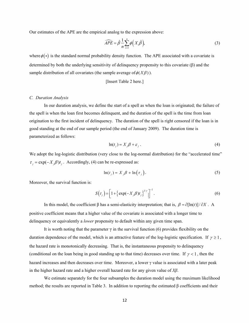
Our estimates of the APE are the empirical analog to the expression above:

( )1

1ˆ ˆ ,n

ii

APE Xn

β φ β=

= ∑ (3)

where ( )φ i is the standard normal probability density function. The APE associated with a covariate is

determined by both the underlying sensitivity of delinquency propensity to this covariate (β) and the

sample distribution of all covariates (the sample average of ( )Xφ β ).

[Insert Table 2 here.]

C. Duration Analysis

In our duration analysis, we define the start of a spell as when the loan is originated; the failure of

the spell is when the loan first becomes delinquent, and the duration of the spell is the time from loan

origination to the first incident of delinquency. The duration of the spell is right censored if the loan is in

good standing at the end of our sample period (the end of January 2009). The duration time is

parameterized as follows:

ln( )j j jt X β ε= + . (4)

We adopt the log-logistic distribution (very close to the log-normal distribution) for the “accelerated time”

exp( )j j jX tτ β= − . Accordingly, (4) can be re-expressed as:

( )ln( ) lnj j jt X β τ= + . (5)

Moreover, the survival function is:

( ) { }11/

1 exp( )j j jS t X tγ

β−

⎡ ⎤= + −⎢ ⎥⎣ ⎦. (6)

In this model, the coefficient β has a semi-elasticity interpretation; that is, [ln( )] /t Xβ = ∂ ∂ . A

positive coefficient means that a higher value of the covariate is associated with a longer time to

delinquency or equivalently a lower propensity to default within any given time span.

It is worth noting that the parameter γ in the survival function (6) provides flexibility on the

duration dependence of the model, which is an attractive feature of the log-logistic specification. If 1γ ≥ ,

the hazard rate is monotonically decreasing. That is, the instantaneous propensity to delinquency

(conditional on the loan being in good standing up to that time) decreases over time. If 1γ < , then the

hazard increases and then decreases over time. Moreover, a lower γ value is associated with a later peak

in the higher hazard rate and a higher overall hazard rate for any given value of Xβ. We estimate separately for the four subsamples the duration model using the maximum likelihood

method; the results are reported in Table 3. In addition to reporting the estimated β coefficients and their

13  

standard errors, we also report the marginal effect of a one-unit change in the covariate (from the mean

values) on the expected median duration of the spell (according to the survival function given by (6)).

[Insert Table 3 here.]

Though the probit and duration analyses are closely related, they examine somewhat different

aspects of the propensity to delinquency. In the probit analysis, all loans that are delinquent at any point

in time during the sample period are treated the same. While the probabilistic results are intuitive, they do

not capture the accuracy of duration, i.e., the time from origination to delinquency. On the other hand, a

duration analysis does not distinguish a pool of loans with a low occurrence of quick delinquency from

another pool of loans with higher delinquency rates but where delinquency tends to occur among more

seasoned loans. For these reasons, the two sets of results complement one another. When they are

mutually consistent, our discussion will focus on the probit results because they are easier to interpret.

The following sections provide a detailed discussion of the results from both tables, along with additional

analyses.

III. Loan Types and Attribution of Differences in Delinquency

This section discusses the differences in loan performance across loan type: origination channel

(Bank vs. Broker) and documentation level (Full-Doc vs. Low-Doc). We further analyze two related

issues: First, which covariates determine a borrower’s choice of loan type? Second, how can we

decompose the differential delinquency rates across loan types into differences due to observable

characteristics versus unobserved heterogeneities?

A. Differences in Loan Performance by Loan Type

A prominent feature of our results is that broker-initiated loans exhibit much higher delinquency

rates than bank-initiated loans, as evidenced by the subsample summary delinquency rates at the bottom

of Table 2. The difference in the probabilities is greater than 10 percentage points, a difference that is

statistically and economically highly significant, indicating serious conflicts of interest in the brokerage

channel where the loan originators’ incentive is to maximize fees and commissions without bearing the

long-term consequences of low-quality loans.

The contrasts among subsamples are even more striking in the duration model. The median

duration times (in months) reported at the bottom of Table 3 reveal that a loan originated with full

documentation by the bank has a median life of 25 years (300 months) before delinquency; the same

14  

median lifetime drops steeply to 8.4 years for Bank/Low-Doc loans, and to 7.9 years for Broker/Full-Doc

loans. Finally, the median life is a mere 4.6 years for Broker/Low-Doc loans.

The comparison of the delinquency propensity between Bank/Low-Doc and Broker/Full-Doc

loans is not straightforward. While the former have a considerably lower overall delinquency rate, their

median time to delinquency is comparable to the latter (the difference is not statistically significant).

Moreover, the γ estimate (reported at the bottom of Table 3) is in fact smaller for the Bank/Low-Doc

subsample than for the Broker/Full-Doc subsample, indicating a higher hazard rate in the former,

conditional on covariates. Such a combination implies that, conditional on delinquency, the borrowers

from the Bank/Low-Doc channel go into delinquency more quickly. Plausibly, a borrower who will

default quickly after loan origination should be easier to screen out than a borrower who defaults years

into the life of the loan. Therefore, low documentation leads to financing some of the more “obvious”

low-quality borrowers.

Certain loan types could be more prevalent in some markets than others. For example, brokers

and low-documentation products may have had greater market penetration in places with booming

markets like California and Florida, where, during the boom, borrowers eager to enter the housing market

tried to qualify for loans they could not afford in order to profit from the rising prices, and brokers

accommodated such demand by issuing easy loans. These are also the areas where, after the market bust,

housing prices plummeted more and delinquency rates were higher than in other parts of the country. A

robustness study including state dummy variables confirms that our results regarding loan types are not

driven by geography. Furthermore, if we exclude loans originated in California and Florida, the average

delinquency rate of the full sample becomes 26.3%, the difference in the delinquency rates between

broker- and bank-originated loans is 11.8%, and that between low- and full-documentation loans is 7.2%.

These numbers are comparable to the corresponding numbers for the full sample, indicating that the

delinquency patterns related to loan types are not unique to a handful of “hot markets.”

B. Choice of Loan Origination Channel and Documentation Level

Differences in loan performance by loan type raise the question of how borrowers select into

different types of loans. Theoretically, a borrower living in any location can apply for a loan directly

from the bank. In regions where the bank does not have branch operations, the loan application can be

completed via phone or internet. Therefore, obtaining a loan from a broker represents a choice made by

the borrower, or a lack of knowledge about available alternatives. The same can be said for choosing a

low documentation loan. Table 4 reports our model results in two panels. Panel A uses only loan and

borrower characteristics as regressors, while Panel B adds neighborhood characteristics to the list of

covariates. The sample size for Panel B is about 25% smaller due to the additional data requirement.

15  

[Insert Table 4 here.]

Column 1 of Table 4 Panel A indicates that the following variables predict a higher likelihood

that a borrower will obtain a loan from a broker rather than from the bank: high debt level, original

purchase (as opposed to refinance), first lien, first-time owner, owner-occupied, low income, low credit

score, female borrower, minority borrower, young borrower, short employment tenure, and self-employed.

All non-white racial groups favor the Broker channel in comparison to whites. Most of these

characteristics (except perhaps the first-lien and self-employed variables) are associated, on average, with

lower financial sophistication, less experience with mortgages, and lower credit quality. This relation

calls attention to the issue of irresponsible lending--lending without due regard to ability to pay, to poorly

informed borrowers--as analyzed by Bond, Musto, and Yilmaz (2008) and Inderst (2006).

The variables that predict choosing a low-doc loan have the following contrasts with those that

predict choosing a broker. First, borrowers with low loan-to-value (LTV) ratios but high loan size are

more likely to choose low documentation. Second, first-time owners and those purchasing owner-

occupied properties are less likely to choose low documentation. Third, borrowers with high income and

credit scores tend to choose low documentation. Fourth, black borrowers do not appear

disproportionately in low documentation loans, while Hispanic and Asian borrowers do. Finally, age is

not correlated with documentation level. To summarize, low documentation loans do not necessarily

attract less-experienced borrowers. The most prominent summarizing feature of these borrowers seems to

be that they are “good on paper.” That is, borrowers who have favorable “hard” information (i.e.,

information that is quantifiable and could potentially be verified, such as LTV, prior mortgage experience,

high income, and high credit score) choose low documentation.

Prior research has shown that lending practices and borrower characteristics are correlated with

neighborhood characteristics (e.g., Calem, Gillen, and Wachter (2004), Nelson (2009)). Table 4 Panel B

reports the relation between neighborhood characteristics and the respective likelihoods that a borrower

will select the broker channel or apply for a low-doc loan. The model’s regressors include average per

capita income (Avgincome) at the zip code level, and also include the following regressors at the census

tract level: Log population size (Population)17, percentage of residents who are black (Pctblack) and

Hispanic (Pcthisp), median age (Medage), and unemployment rate (Unemprate). All regressors included

in the model reported in Table 4 Panel A are also included in the model reported in Panel B, but are not

tabulated for economy of space.

Brokers seem to predominate in neighborhoods with low minority representations and young

residents. The combination of results from Panels A and B indicates that minority households in non-

minority neighborhoods are the prime clients of mortgage brokers. Low documentation loans, on the                                                             17 The average and median population size of a census tract is between 5,000 and 6,000 residents.

16  

other hand, are significantly more popular in minority neighborhoods and in booming neighborhoods

(with low unemployment rates) with young populations.

C. Decomposition of Pairwise Subsample Differences in Delinquency

When researchers try to examine the effect of a variable, they often include the variable as a

regressor and estimate its contribution in explaining the outcome. Following this logic, we could estimate

a regression model that includes loan type as a regressor:

* ,i i i iDelinquency X LoanTypeβ λ ε= + + (7)

where LoanType indicates the origination channel or documentation status. We refrain from conducting

such an analysis because a specification like (7) is meant to capture a “treatment effect,” where the

relevant question is: if two ex ante identical borrowers--along both observable and unobservable

dimensions--were assigned to different loan types, how would their delinquency propensity differ ex post?

We argue that there is no conventional “treatment effect” of the loan types in our context because

all loans are serviced by the bank, regardless of the origination channel and documentation level. As a

result, any difference in the outcome that is correlated with loan type should be attributed solely to the

“selection effect”; that is, borrowers of different observable and unobservable characteristics are attracted

to different loan types, and such characteristics are correlated with delinquency propensities.

The dichotomy between observable qualities and unobserved heterogeneities has implications for

understanding why delinquency rates vary across subsamples. For example, if the higher delinquency

rates in the Broker subsamples are predictable from observed characteristics (such as LTV and credit

score), we could conclude that the Broker channel serves an observably lower-quality clientele, or applies

looser lending standards than the Bank channel. If unobserved heterogeneity is responsible for the

difference, then we infer that the Broker channel is subject to more severe adverse selection among

potential borrowers along unobserved or unquantifiable dimensions (such as income stability, or hidden

expenditures), presumably because mortgage brokers are less diligent than bank employees in using

additional hard or soft information to screen borrowers. The same logic applies to the Full-Doc/Low-Doc

comparison.

While our study confirms earlier results by Alexander, Grimshaw, McQueen, and Slade (2002)

who document higher delinquency rates among brokered loans compared to loans originated through the

bank’s retail channel, that earlier study does not contain the level of borrower detail used in this study and

hence cannot decompose the difference across loan origination channels into differences due to

characteristics observable to the bank versus unobserved heterogeneity. We apply a non-linear version of the Blinder-Oaxaca (1973) decomposition to the probit model to

separate the effects of observable qualities from the effects of unobserved heterogeneities. Let D = {0, 1}

17  

be the index for the two subsamples for comparison, and let Y be the indicator variable for loan

delinquency. More specifically, we will compare loans from the Bank (D = 0) and Broker (D = 1)

channels, controlling for the documentation level, and loans issued as Full-Doc (D = 0) and Low-Doc (D

= 1), controlling for the origination channel. We obtain coefficient estimates for all subsamples from the

probit model as specified in equation (1) and reported in Table 2.

The difference in the delinquency rates between two subsamples can be expressed as:

{ } { }0 0 1 0

( | 1) ( | 0)

( ) | 1 ( ) | 0 ( ) ( ) | 1

E Y D E Y D

E X D E X D E X X Dβ β β β

= − =

⎡ ⎤ ⎡ ⎤ ⎡ ⎤= Φ = − Φ = + Φ −Φ =⎣ ⎦ ⎣ ⎦ ⎣ ⎦, (8)

or as:

{ } { }1 1 1 0

( | 1) ( | 0)

( ) | 1 ( ) | 0 ( ) ( ) | 0

E Y D E Y D

E X D E X D E X X Dβ β β β

= − =

⎡ ⎤ ⎡ ⎤ ⎡ ⎤= Φ = − Φ = + Φ −Φ =⎣ ⎦ ⎣ ⎦ ⎣ ⎦. (9)

Equations (8) and (9) are numerically different but employ the same logic. The left sides of the

equations are the difference in the expected value of the outcome variable (delinquency) between the two

subsamples. The right sides of the equations feature a sum of two terms. In labor economics, the first

term is called the “endowment effect”; that is, the difference in the outcome due to different distributions

of the covariates (the X variables) in the two subsamples. The difference due to the endowment is

isolated by using the same set of coefficients for both subsamples. The second term is called the

“coefficient effect” (in a production function, the coefficients are also referred to as “returns to factors”)

and estimates the hypothetical difference in delinquency if the two subsamples had identical covariate

distributions but the coefficients remained different. The coefficient effect encompasses two possibilities:

a differential sensitivity of the outcome to the covariates in the underlying model, or the effects of missing

variables that spill over to the remaining covariates. Both possibilities reflect unobserved heterogeneity.

Equations (8) and (9) differ only because they use a different subsample as the “base” sample.

There is no a priori argument to favor using one subsample versus the other as the base, so we report both

sets of results in Table 5. Table 5 Panel A reports the comparison of Full-Doc (D = 0) versus Low-Doc

(D = 1) loans separately for the Bank and Broker channels. The total difference (the left sides of the

above equations) is reported in the bottom row, and is, by construction, 100% of the difference. The

“Low-Doc sample as benchmark” comparison applies equation (8) and uses the D = 1 subsample as the

base; the “Full-Doc sample as benchmark” comparison applies equation (9) and uses the D = 0 subsample

as the base. The t-statistics are based on standard errors obtained through the block bootstrap clustered at

the MSA level.18

                                                            18 The conventional delta method for computing standard errors does not apply. The estimator is a function of the model coefficients that depends on the sample distribution of covariates, and thus is a stochastic function of the

18  

[Insert Table 5 here.]

The two sets of results are qualitatively similar, so we focus on the first set of results (equation

(8)) for discussion. Conditional on the Bank (Broker) channel, Low-Doc loans have, on average, a

delinquency rate that is 4.8 (8.0) percentage points higher than for Full-Doc loans. Almost 100% of this

difference should be attributed to the “coefficient effect”. The estimated “endowment effect” is small and

is not statistically significant; if anything, the “endowment effect” indicates that Low-Doc loans are of

slightly better observed quality. We conclude that Low-Doc loans are just as “good on paper” as Full-

Doc loans, but encompass more adverse selection along unobserved dimensions.

The comparison between Bank and Broker loans conditional on documentation level (reported in

Table 5 Panel B) offers a different picture. Here, the endowment effect accounts for three-quarters (over

half) of the total difference in delinquency rates between Bank and Broker loans using the Broker (Bank)

subsample as the base sample. Put differently, if the bank and its brokers had loaned to borrowers of the

same observable quality, more than half of the difference in the incremental delinquency rate between the

Broker and Bank subsamples (10.4 percentage points for Full-Doc, and 13.6 percentage points for Low-

Doc) would have disappeared.

The implications stemming from the higher delinquency rates among Broker and Low-Doc loans

are markedly different. The Low-Doc channel does not necessarily compromise lending standards along

verifiable metrics (such as LTV and credit score), but suffers from less careful verification of some

reported information (such as income and owner-occupancy status), or less diligent screening of

borrowers along hard-to-quantify measures (such as other major expenditures).19 On the other hand, the

Broker channel--while also lacking incentives for careful screening--penetrated a borrower pool that was

of significantly worse quality, even by observable, quantifiable, and potentially verifiable standards.

The following hypothetical example illustrates the differences in borrower profiles across loan

type. Suppose Borrower A has a high credit score and high income but has major withholding from his

income (such as alimony); Borrower B has high income that is difficult to verify (because he is self-

employed) or is unwilling to reveal his true income (because of tax reasons); and Borrower C has a low

credit score and does not have a stable job or income. Our analysis predicts that borrowers A and B are

more likely to choose low-doc loans, while Borrower C is more likely to approach (or be approached by)

a mortgage broker.

                                                                                                                                                                                                coefficients. In contrast, the delta method applies when the estimator is a nonstochastic function of the model coefficients. 19 Often cited reasons for choosing low-documentation loans include prior bankruptcy, income that was not reported to the IRS, and other financial complications such as divorce or pending legal issues.  

19  

Among all borrower characteristics, credit score has the highest predictive power for delinquency

and is verified for full-documentation as well as for low- or no-documentation loans. Exploring the

relationship between credit score and other covariates sheds additional light on the composition of

borrowers in different subsamples. The results we report in Table 6 confirm our interpretation of results in

Tables 4 and 5. We find that Low-Doc borrowers have, on average, higher credit scores than Full-Doc

borrowers. Moreover, credit score and reported income and cash reserves are strongly related in the Full-

Doc subsamples, but the relation is much weaker in the Low-Doc subsamples. The fact that reported

income and cash reserves may not be certified in the Low-Doc subsample may explain their weakened

relationship with credit score, an issue we discuss in more detail in Section IV.

[Insert Table 6 here.]

An examination of credit scores by race reveals that average credit scores are highest among

Asian and white borrowers, and lowest among Hispanic and black borrowers. Hispanic borrowers who

obtain loans directly from the bank have credit scores that are comparable to those of white borrowers,

but those who obtain loans through a broker have credit scores that are on average 2-5 points lower.

Black borrowers have average credit scores that are 14-27 points lower than white borrower credit scores,

across all subsamples.

Last, the time trend of credit scores, as shown by the year dummy variable coefficients, is

informative; while Bank loans saw steady improvement in credit scores over time from 2004-2008, credit

scores for Broker loans deteriorated from 2004-2007, and only recovered in 2008. The findings provide

evidence that the bank pursued a growth strategy which relied on penetrating marginal borrowers through

the broker channel.

D. Differences within the Broker Channel

We differentiate within the Broker channel between pure brokers and correspondents. Pure

brokers act as matchmakers and submit loan applications to a variety of banks for competitive pricing. In

contrast, the correspondents in our sample have long-term, established, and near-exclusive relationships

with the bank for at least one product type (such as prime loans) and abide by the bank’s particular

underwriting guidelines in exchange for expedited loan processing. Correspondents in our sample close

loans in their own name using a warehouse line of credit advanced by the bank, and then quickly re-sell

the loans to the lending bank. Due to the longer and more exclusive relationships, the incentives of the

correspondents are more aligned with that of the bank than pure brokers.

To examine the difference between the two groups of brokers, we estimate the probit model

(equation (1)) for correspondents and non-correspondents separately, interacted with the Full-Doc/Low-

Doc sorting. The double sorting produces four subsamples. We report the results in Table 7.

20  

[Insert Table 7 here.]

A comparison of Table 7 to Table 2 confirms our conjecture. The patterns revealed in the

Correspondent subsamples are always between those of the Bank subsamples and those of the Non-

Correspondent subsamples, and tend to be closer to the former. For example, total delinquency rates for

Correspondent loans are marginally higher than for Bank loans (5 percentage points higher for both Full-

Doc and Low-Doc loans), but are much lower than for the Non-Correspondent subsamples (5.7

percentage points lower for Full-Doc, and 15.1 percentage points lower for Low-Doc). Also, there are

more commonalities in the relations between loan performance and individual covariates among the Bank

and Correspondent subsamples than among the Correspondent and Non-Correspondent subsamples.

IV. Liar’s Loan: Model Predictive Power and Information Falsification

The “liar’s loan” problem includes various forms of borrower information falsification, possibly

at the encouragement of brokers who have stronger incentives to close deals than to screen applicants.

Such falsification appears primarily among low- or no-documentation loans, where much of the recorded

information is self-reported without strict verification. Anecdotal evidence20 suggests that the following

falsifications are among the most common: exaggerating income or assets, hiding other major

expenditures, and claiming that properties purchased for investment/speculation purposes will be owner-

occupied as primary residences.

Despite the mounting anecdotes, there are no formal empirical analyses of borrower information

falsification and its impact on loan performance. Our paper fills this void by presenting two pieces of

analysis. First, we use model predictive power as an aggregate measure of the quality of information

recorded at loan origination. Second, we offer evidence of the falsification of individual variables by

exploring how their relationship to loan performance differs between the Full-Doc and Low-Doc

subsamples.

A. Model Predictive Power across Different Loan Types

Inaccurately recorded loan and borrower characteristics, whether due to unintentional mistakes or

due to intentional falsification, will attenuate the empirical relationship between these variables and loan

performance, thereby compromising the model’s fit and predictive power. Because the bank services and

                                                            20 See, for example, “My Personal Credit Crisis” by Edmund Andrews, which appeared in the New York Times on May 17, 2009. The author provides a detailed description of his personal experience in qualifying for a loan far beyond his financial means by hiding, forging, and strategically managing information with the help of his mortgage broker.

21  

maintains records for all loans in our sample, there is no obvious reason to believe that incidences of

random data recording error should vary systematically across the subsamples after loan origination. This

leaves intentional falsification (including hiding) of information as the most plausible explanation for

differences in model predictive power across loan type.

In Tables 2 and 3, we observe that the goodness-of-fit (i.e., the in-sample model predictive power)

is indeed substantially different across the four subsamples. More specifically, the two Full-Doc

subsamples have much higher pseudo R-squared statistics (22.1% and 18.2% for Bank and Broker

subsamples using probit, or 17.4% and 16.2% using duration, respectively) than the two Low-Doc

subsamples (13.6% and 14.6% using probit, or 14.1% and 14.5% using duration), indicating higher

quality explanatory variables in the Full-Doc subsamples. Here the reported pseudo R-squared is

0(1 ln / ln )L L− , where lnL is the maximized log likelihood value of the probit or duration model using all

covariates, and lnL0 is the maximized log likelihood value of the same model on the same sample, but

with a constant as the sole regressor.

The pseudo R-squared discussed above is the most popular goodness-of-fit measure for non-

linear models for which there are no obvious empirical analogs to the residuals. Nevertheless, it suffers

from two major drawbacks. First, it does not have an interpretation as intuitive as the R-squared metric

for linear models, which indicates the percent of variation explained. Second, the in-sample goodness-of-

fit should not be equated with model predictive power. When economic agents (the bank or mortgage

brokers) make decisions, their predictions are based on information revealed at the time, without

knowledge of the full sample. Therefore, an out-of-sample prediction method is more appropriate for our

research purposes, because it avoids the look-ahead bias. With these two issues in mind, we develop the

following “excess percentage of correct predictions” measure to assess the predictive power of the probit

model.

Let Pi denote the predicted probability of delinquency for the i-th observation, where the

prediction is made out-of-sample (to be described in more detail later). Let Yi denote an indicator variable

for delinquency, and let p denote a cutoff value. Then the objective to maximize “correct predictions”

can be expressed without loss of generality as:

S =ωS1 + 1−ω( )S2 −α =ω Pr(P i≥ p |Yi = 1) + 1−ω( )Pr(P i< p |Yi = 0) −α (10)

for some (0,1)ω∈ , which reflects the relative importance of a type-I error (failure to predict a delinquent

loan) and a type-II error (mistakenly predicting that a non-delinquent loan will be delinquent); α is a

22  

constant representing the maximum probability of obtaining a correct prediction with a random guess .

The maximization of (10) has a unique solution of p :21

[ ]

(1 ) ( )1 ( ) (1 ) ( )

E YpE Y E Y

ωω ω

−=

− + −. (11)

A natural choice of ω is 1/2, where the objective function weights the two types of prediction

errors equally. Under such a criterion, equation (11) simplifies to ( )p E Y= , with the corresponding

empirical analog being the sample frequency of delinquency revealed at the time of the evaluation.22

According to this rule, we classify a loan as “predicted to be delinquent” if the out-of-sample predicted

probability exceeds the time-adapted sample frequency of delinquency.

Such a classification method has the desirable feature of coinciding with the likelihood ratio rule

if the probit model is correctly specified. Let fD ( fND) be the density functions of the predicted probability

of delinquency for the subsample of loans that are ex post delinquent (non-delinquent). Then for any

value v, fD(v) > fND(v) if and only if v > E(Y), as long as the model is correctly specified, i.e., as long as

equation (1) holds with the residual ε normally distributed. In other words, the two density functions fD(v)

and fND(v) have a single crossing at v = E(Y). As a result, Pi > E(Y) implies that the i-th observation is

more likely to be drawn from the subsample of ex post delinquent loans than from that of the ex post non-

delinquent loans, and therefore should be classified as “predicted to be delinquent” based on the relative

likelihood. The opposite applies when Pi < E(Y).23

Finally, the percentage of correct predictions should be judged against the benchmark of a non-

informative model, which produces correct predictions half of the time in expectation when ω = 1/2. As a

result, we set α = 1/2 in equation (10) to obtain the “excess percentage of correct predictions.”24

We use the following empirical procedure to calculate the out-of-sample excess percentage of

correct predictions. First, we divide each of the four subsamples into semi-year segments by the loan

origination date, and pick one semi-year segment at a time to measure the accuracy of the model

predictions. We call this the “test sample/period.” Second, for each “test period,” we use all information

available up to just before the test period to estimate the model in equation (1) without the year dummy

variables25; we call this the “estimation sample/period.” It is important to emphasize that not only do the

loans in the estimation sample have to be originated before the test period, but their delinquency status

must also be assessed at the beginning of the test sample period. Third, we apply the predictive model                                                             21 The proof of equation (11) is in the appendix. 22 Another natural choice of ω is Pr[Y=1]=E(Y), which would lead to maximizing the un-weighted fraction of predictions correctly predicted. Under such a criterion, equation (11) simplifies to 1/2. 23 The proof of this argument is in the appendix. 24 For general values of ω, the corresponding α parameter is equal to max(1- ω, ω). 25 Time dummy variables should be omitted from any out-of-sample predictions because they are not applicable for future samples.

23  

using the coefficients estimated from the estimation sample on the test sample to form the predicted

probability of delinquency. Finally, equation (10) formulates the calculation of the final measures.

Table 8 reports the percentage of correct predictions by subsample for each semi-year, separately

for S1, S2, and S as defined in equation (10). The test periods start from the first half of 2005 to allow for

a prior estimation period.

[Insert Table 8 here.]

Two patterns evident in the table warrant further discussion. First, loan documentation type--not

loan origination channel--is the key determinant of the model’s predictive power. Figure 4 depicts model

predictive power by plotting the time series of the excess percentage of correct predictions (S) by loan

type. The model’s predictive power in the Bank/Full-Doc and Broker/Full-Doc subsamples is

indistinguishable in each semi-year; the same can be said about the model’s predictive power in the

Bank/Low-Doc and Broker/Low-Doc subsamples. More importantly, the model’s predictive power in the

Full-Doc subsamples is substantially higher than for the Low-Doc subsamples. The across-time averages

are as follows: Bank/Full-Doc (17.2%), Bank/Low-Doc (11.5%), Broker/Full-Doc (18.1%), and

Broker/Low-Doc (11.1%). Such a contrast suggests that low documentation loans may allow some

borrowers to falsify information in order to qualify for loans or obtain more favorable loan terms. As a

result, some of the variables in the regressions could contain measurement errors, compromising their

predictive power.

[Insert Figure 4 here.]

Second, the predictive power of the model--especially for the Full-Doc subsamples—declined

from 2005 to 2006, before rebounding slightly in 2007. This trend suggests that loans originated during

the boom period experienced positive shocks in delinquency that could not be predicted by their

characteristics based on information available at the time of loan origination. Rajan, Seru, and Vig (2009)

also find that the predictive power of credit score and LTV deteriorated during the high securitization

period.26 The difficulty in predicting loan performance based on observed characteristics for loans

originated in 2006 indicates the bank may not have been aware it was originating low-quality loans during

that time period; this explains why the bank did not tighten its lending standards until 2007, when it began

to incur losses from loans originated during the boom.27

B. Evidence of Borrower Information Falsification from Individual Variables

                                                            26 We find that the deterioration in model predictive power is more prominent among full-documentation loans, while Rajan, Seru, and Vig (2009) found it to be stronger among low documentation loans. The difference could be due to our use of a larger set of covariates in the prediction and a different metric of model predictive power, and our use of a more recent sample which begins and ends later than theirs. 27 Please also see Figure 3.

24  

B1. Overview

The model’s lower predictive power for Low-Doc subsamples relative to Full-Doc subsamples

provides strong evidence that the information recorded for low-documentation loans is of lower quality.

The lower predictive power is an aggregate measure of the quality of the recorded information, but it does

not reveal which particular variables are mis-measured. We now present evidence that borrowers of low-

documentation loans tended to falsify particular variables, especially income. We find that such

falsification is especially prominent among Broker/Low-Doc loans.

Due to both incentives and the reporting system, falsification is most likely to occur in the

following variables. First, borrowers purchasing a second home or investor property could falsely claim

that the property will be owner-occupied and used as a primary residence, thereby securing a lower

interest rate. While lenders are often able to verify occupancy status for refinance loans by requiring the

borrower to submit proof of residence (such as utility bills), lenders are unable to verify occupancy status

for home purchase loans at origination. Occupancy fraud is often cited as a major contributor to the surge

in delinquencies, as borrowers became over-leveraged from holding multiple mortgages.

Second, low-documentation loans enabled borrowers to falsify employment information--

including employment tenure and self employment status--as well as income, asset, expense, liability, and

debt information. For many low-documentation loans, lenders do not verify borrowers’ financial

conditions by requiring a history of bank statements, W-2 forms, asset documentation (such as retirement,

savings, or investment account information), or outstanding debt documentation (including student loan

information, mortgage statements, credit card statements, and information on judgments/liens resulting

from legal action). Borrowers who want to qualify for higher loan amounts or more desirable loan terms

through a lower reported debt-to-income ratio could overstate their income and assets, and/or understate

expenses and other debt liabilities.

B2. Income Falsification

The coefficients on Income in Tables 2 and 3 support the hypothesis that reported income was

often falsified by borrowers of Low-Doc loans.28 In the Full-Doc subsamples, higher income is

significantly and negatively associated with delinquency, as measured by both lower probability of

delinquency and longer duration to delinquency conditional on all other attributes. However, the sign on

the Income coefficient switches in the Low-Doc sub-samples. Moreover, the coefficients are particularly

strong in the Broker/Low-Doc subsample where higher income is associated with significantly higher

propensity for delinquency. The most plausible explanation for this contrast is that, when income is not

verified, higher income (conditional on all other attributes) may more often be the result of exaggeration

                                                            28 In the regression, the Income variable is coded as zero when it is missing, and the dummy variable for missing income information, IncomeMiss, is set equal to one.

25  

rather than financial strength. Reported income will have a positive sign in the delinquency prediction

regressions if the incentive to exaggerate income is negatively correlated with individual credit quality.

The dummy variable for missing income information, IncomeMiss, offers corroborative evidence.

In the Bank/Full-Doc and Broker/Full-Doc subsamples, only 0.6% and 0.9% of the observations have

missing income information, and in these subsamples missing income information does not predict loan

performance. Thus, in the Full-Doc subsamples, the sporadic cases of missing income information most

likely result from data recording error and not from falsification. In contrast, income is missing for 10.3%

and 9.2% of the observations in the Bank/Low-Doc and Broker/Low-Doc subsamples, respectively.

Missing income information significantly predicts higher delinquency propensity in the Broker/Low-Doc

subsample, where missing income information is associated with a 4.7 percentage point increase in the

probability of delinquency, or an 8 month reduction in the time from loan origination to delinquency. The

same effect is present but not significant in the Bank/Low-Doc subsample. Thus, purposefully not

reporting income information is a low-documentation-only phenomenon. Presumably, borrowers with

low or irregular incomes in the Low-Doc subsamples are more likely than comparable High-Doc

borrowers to exaggerate or omit their incomes on the loan application.29

In comparing Table 2 and Table 7, it is worth noting that the various perverse relations discussed

above for broker-originated loans are mostly driven by non-correspondent brokers. This evidence

suggests that correspondents are far less likely to encourage or accommodate borrower information

falsification than non-correspondents because the former have stronger reputation concerns due to their

exclusive or long-term relationships with the bank.

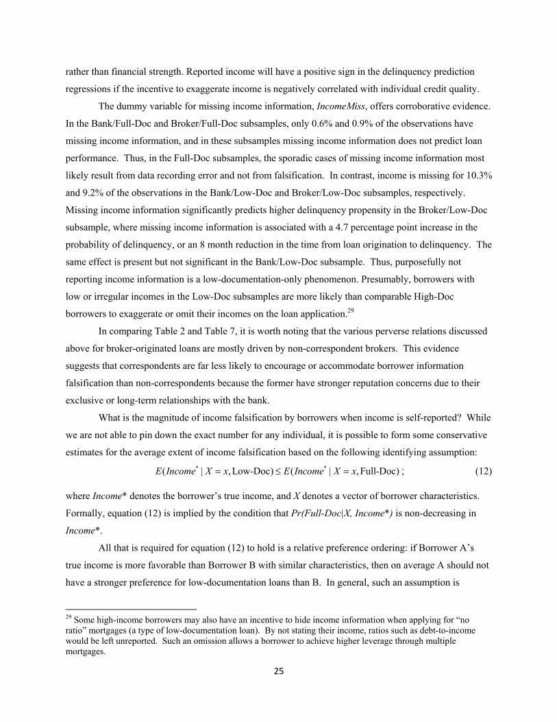
What is the magnitude of income falsification by borrowers when income is self-reported? While

we are not able to pin down the exact number for any individual, it is possible to form some conservative

estimates for the average extent of income falsification based on the following identifying assumption:

* *( | ,Low-Doc) ( | ,Full-Doc)E Income X x E Income X x= ≤ = ; (12)

where Income* denotes the borrower’s true income, and X denotes a vector of borrower characteristics.

Formally, equation (12) is implied by the condition that Pr(Full-Doc|X, Income*) is non-decreasing in

Income*.

All that is required for equation (12) to hold is a relative preference ordering: if Borrower A’s

true income is more favorable than Borrower B with similar characteristics, then on average A should not

have a stronger preference for low-documentation loans than B. In general, such an assumption is

                                                            29 Some high-income borrowers may also have an incentive to hide income information when applying for “no ratio” mortgages (a type of low-documentation loan). By not stating their income, ratios such as debt-to-income would be left unreported. Such an omission allows a borrower to achieve higher leverage through multiple mortgages.

26  

plausible because a high certified income is more likely to result in lower interest rates or more favorable

loan terms on full-documentation loans, while some of these benefits are forfeited in low-documentation

loans because the sensitivity of loan pricing to uncertified income is lower. Self-reported income could

still materially affect the qualification of the loan application, providing an incentive for falsification.

The only group for whom equation (12) may plausibly not hold is the self-employed. Self-

employed borrowers disproportionately choose low-documentation loans (see the more detailed analysis

in Section III and the results in Table 4), not necessarily because they want to exaggerate their income but

because their income is often difficult to certify (e.g., they do not have W-2 forms) or they do not wish to

reveal their true cash flows for tax reasons. We therefore exclude the self-employed from our estimation

of the extent of income exaggeration among borrowers of low-documentation loans.

Our first estimate of the extent of income exaggeration comes from simply comparing borrower

income (at the household level) to the average income of the neighborhood where the property is located.

We obtain the average per capita adjusted gross income information at the zip code level from the Internal

Revenue Service's Individual Master File (IMF) system for the years 2004, 2005, and 2006. A zip code

area has, on average, 2,326 households, and the average household size is 3.3 people. We use 2006 data

for loans originated in the post-2006 years. The average ratios of borrower household income to the

neighborhood average income per capita are 3.6 and 3.3 for the two Full-Doc subsamples, and are

considerably higher at 4.3 and 3.8 for the two Low-Doc subsamples. Thus, assumption (12) implies that

the average degree to which low-documentation borrowers exaggerate their income is at least 16%-19%,

if their true income stands at a ratio to their neighborhood average that is no higher than their full-

documentation counterparts.

A more refined estimate incorporates borrower demographics in addition to neighborhood

attributes to proxy the true income (Income*). Suppose a borrower’s Income* can be expressed as a

linear function of borrower characteristics, neighborhood characteristics, year dummies and an error term,

with the error term mean independent of covariates conditional on documentation status. Then such a

function could be estimated reliably using the sample of full-documentation loans because there should be

no systematic bias in the recorded income given that it is certified; hence, Income ≈ Income*. Below is

the regression output from full-documentation loans, where the dependent variable is the reported (and

certified) household monthly income in $1,000 units and the t-statistics are reported below the

coefficients.

27  

0.014* 0.846* 0.651*ln( ) 0.416*[18.01] [ 16.49] [13.31] [ 1.92]

0.430* 0.575* 0.051* 0.030* [-4.31] [5.04] [4.40] [ 2.15]

0.131* 2005 0.373*

Income CreditScore Female Age Hispanic

Black Asian AvgIncome Unemprate

Y

= − + −− −

− + + −−

+ + 2006 0.299* 2007 0.010* 2008[2.58] [5.40] [4.76] [0.096]

R-squared: 6.9%; number of observations: 138,514.

Y Y Y+ + (13)

All coefficients in the above regression are intuitive. Older borrowers and borrowers with higher

credit scores tend to have higher income. Female borrowers have lower income on average.30 Black and

Hispanic borrowers have lower income on average than white borrowers, and Asian borrowers as a group

have the highest income. In addition, borrower income is significantly and positively correlated with the

zip-code area average income (AvgIncome) and negatively correlated with the census tract unemployment

rate (Unemprate). Finally, overall borrower income grew from 2004 (the omitted year in the regression)

to 2006, and then decreased afterwards.

Resorting to the identifying assumption of (12)--which presumes that the error term from

regression (13) is not positively correlated with Low-Doc status--we can estimate the upper bound for the

expected true income of low-documentation borrowers by applying the estimated coefficients from (13)

to the covariates of these borrowers. We generate an “income exaggeration” variable to capture the

difference between the reported Income and the estimated Income*. We find that in dollar terms the

average (median) income exaggeration is $1,830 ($753) per month; in percentage terms, the average

(median) low-documentation borrower reports income that is 28.7% (20.0%) above their estimated true

income level. Given that these estimates err on the conservative side, the data suggest serious income

falsification among low-documentation borrowers from the benchmark of full-documentation borrowers.

The correlations between estimated true income, estimated income exaggeration and loan

performance are all highly statistically significant, and reveal more about the incentives for and

consequences of income falsification. First, the correlation between the estimated true income and

estimated income exaggeration in percentage terms is -7.9%, indicating a stronger incentive to inflate

income when the true income is lower. Second, the correlation between the estimated true income and ex

post delinquency is -23.5%, recovering the normal inverse relationship between income and delinquency

in the Low-Doc subsample that was perverted using reported income (see Tables 2 and 3). Finally, as

expected, the correlation between estimated income exaggeration and ex post delinquency is positive at

                                                            30 This gender effect is not primarily due to the male-female wage gap, but rather to the fact that a female being listed as the sole borrower is a proxy measure for a female head of household; female-headed households have lower income on average than male-headed households.

28  

8.2%. In other words, delinquency risk increases when borrowers inflate income to obtain a loan beyond

their true means.

B3. Evidence of Other Information Falsification

Additional important variables for delinquency prediction, which potentially can be falsified in

the absence of certification, are OwnerOccupied (a dummy variable for whether the property is owner-

occupied as a primary residence) and CashResv (the borrower’s cash reserves in multiples of the monthly

mortgage payment, in logs). Mortgages on owner-occupied properties are usually considered to be safer

than properties purchased as investments or second homes; the latter are often purchased by borrowers

who have higher combined leverage and who have a lower cost of “walking away” from a mortgage that

has negative equity value. Cash reserves help pull households through temporary negative income shocks

without disrupting mortgage payments.

The coefficients on both variables in Tables 2 and 3 reveal patterns that are generally intuitive:

owner occupancy and high levels of cash reserves are associated with significantly lower delinquency

propensity. However, the coefficients that represent sensitivity of delinquency propensity to both

variables are stronger in the Full-Doc subsamples than in the Low-Doc subsamples,31 and the difference is

more evident using the duration method than the probit model. Hence, there is some evidence that Low-

Doc borrowers may not always truthfully report owner occupancy status and cash reserves, thereby

lowering the explanatory power of these variables. Yet the evidence is weaker and less conclusive than

that regarding income falsification.

Our conversations with bank officials yield two explanations for the higher quality of cash

reserve information relative to income information in explaining delinquency. First, borrowers and

brokers have better information about how income affects loan qualification and pricing, so they have a

stronger incentive to falsify income. Second, verification of assets is often better than that of income

because asset statements are more available than proof of income for a large group of borrowers,

especially those who are self-employed or cash compensated.

V. Loan Types and Loan Pricing

The previous sections show that loans originated via the broker channel and with low-

documentation requirements are of lower quality due to heterogeneity in both observable and

unobservable characteristics, including likely information falsification among low-documentation loans.

An important question thus arises regarding whether market participants were aware of such differences

                                                            31 For this context, we resort to the comparison of the β coefficients in equations (1) and (2), rather than the partial effects. This is because the partial effects are a function of both the sensitivity of the outcome to the regressor (the coefficients) and the subsample average outcomes (delinquency rates). See equation (3).

29  

ex ante, and whether loan pricing (the loan interest rate) adequately reflects the additional risk associated

with brokered and low-documentation loans.

Table 9 addresses this question by (1) analyzing the determinants of interest rates with loan types

as the key regressors of interest; and (2) by analyzing the determinants of delinquency rates including

both loan type and interest rates as regressors. Our full sample consists of a mixture of fixed-rate loans

(47% of the sample) and various adjustable rate loan products. The interest rates on many of the

adjustable rate loans had not yet aged out of the initial rate period by the end of the sample period.

Therefore, we conduct our analyses separately on two subsamples: the set of all fixed rate loans where

the initial interest rate (InitialRate) is informative about loan pricing32, and the set of all adjustable rate

loans where the rate at the end of our sample period (CurrentRate) is different from the InitialRate. In the

latter case, CurrentRate approximates the effective rate that the borrower pays after the introductory rate

expires. Control variables include all regressors that appear in the delinquency prediction analysis as

reported in Tables 2 and 3.

[Insert Table 9 here.]

Most of the coefficients on the control variables are intuitive. That is, variables that are

associated with higher delinquency rates also tend to command higher interest rates. The only exceptions

are loan size (Loan), second lien (SecondLien), and refinance (Refinance); these variables predict higher

delinquency rates but are associated with lower interest rates. The results for these three variables can be

interpreted using a reverse causality argument: when facing low interest rates, borrowers tend to borrow

more, take additional loans, or refinance existing loans.

It is worth noting that federal law prohibits loan pricing based on demographic information

including race/ethnicity. Although some coefficients on these variables are statistically significant, the

economic magnitude is quite small. Take the largest such coefficient as an example: for fixed rate loans,

black borrowers pay an additional 12.5 basis points in the interest rate compared to white borrowers

controlling for observable information (column (1) of Table 9). Yet given the average (median) unpaid

balance on loans among black borrowers of $185,000 ($150,000), the estimated black-white difference in

interest rate amounts to an additional monthly payment of $19 (or $16) using the mean (or median)

balance. It is unlikely that such a payment difference could be pivotal in loan delinquency.

Most important are the coefficients on loan types. With the Bank/Full-Doc category serving as

the benchmark (the omitted category), Columns (1) of Table 9 shows that among fixed rate loans, low-

documentation loans command interest rates that are 29 basis points higher on average ($55 more in

monthly payments for a median sized loan), regardless of the origination channel; Broker/Full-Doc loans

                                                            32 The other important variable determining the interest rate is loan maturity. The vast majority (93%) of our sample has uniform maturity of 30 years. See footnote 15.

30  

command rates that are six basis points higher on average ($6 more in monthly payments for a median

sized loan). The rate premium is modest for low-documentation loans considering the adverse selection

involved. It is almost non-existent for brokered loans, which is more alarming given the double-digit

differences in delinquency rates between bank- and broker-originated loans (see Table 2). Column (3) of

Table 9 presents results for the subsample of adjustable rate loans with rates that had been re-set by the

end of the sample period. Surprisingly, rates are lower for the three types of loans that are of lower

quality in comparison to Bank/Full-Doc loans. Most strikingly, the current interest rates on brokered

loans are 69-77 basis points lower than on Bank/Full-Doc loans. On the other hand, the comparison of

interest rates between the Full-Doc and Low-Doc subsamples is mixed.

Brokers are more likely to originate adjustable-rate loans than banks: 54% of all brokered loans

carry adjustable rates, in comparison to 48% of bank-originated loans. The lower current interest rates on

brokered loans may thus reflect that fact that brokered adjustable-rate mortgages tend to start with more

lucrative “teaser rates” (the average InitialRate for brokered loans is 60-80 basis points lower), and that

some of the current rates may not reflect the fully-adjusted levels (though they have already adjusted from

the initial rate as required by the construction of the subsample). In sum, there is no evidence that

brokered and low-documentation loans are priced higher in the subsample of adjustable rate loans during

our sample period.

Columns (2) and (4) confirm that the loan pricing for brokered and low-documentation loans does

not compensate for their additional risk. Among fixed-rate loans, delinquency rates for the Bank/Low-

Doc, Broker/Full-Doc, and Broker/Low-Doc subsamples are 4.4, 1.3, and 8.6 percentage points higher

than that of the benchmark category (Bank/Full-Doc), controlling for loan characteristics as well as the

interest rate. These differences are both statistically and economically significant. The results are even

stronger for the subsample of adjustable rate loans when controlling for the current interest rate.

In comparison, LaCour-Little (2009) shows that brokered loans tend to have interest rates that are

20 basis points higher than loans available directly from retail lenders. Similar to our finding, Alexander,

Grimshaw, McQueen, and Slade (2002) show that the agency cost risk associated with brokers was not

priced during the period with low default. But they also show that the rate premium surged to more than

200 basis points after such risk was recognized. The same figure is much lower in our study. In addition

to having a different sample, our study controls for more detailed borrower characteristics which drives

down the coefficient on Broker in the loan pricing equation because brokered loans tend to have lower

observable quality as measured by borrower characteristics. In fact, if we drop borrower characteristics

variables that were not included in previous studies, the rate premium for the broker channel would

increase to 36-64 basis points.

31  

Our analysis raises the question of why this major mortgage bank—as well as other market

players—issued lower-quality loans without adequately pricing the additional risk, and allowed the

deterioration in borrower and loan quality to persist before tightening its lending standards. One possible

explanation is information. While it is obvious in 2009 that brokered and low-documentation loans are

more delinquency-prone, the differences were not significant in the early part of the sample period when

the overall delinquency rates were low. The delinquency rates for all outstanding loans were no higher

for brokered loans than for bank-originated loans until 2006, and it was not until 2007 that low-

documentation loans began to exhibit delinquency rates that were considerably higher than those of their

full-documentation counterparts.

This explanation in only partially supported by data. We repeat the analysis on fixed-rate loans

using a subset of loans originated after July 1st, 2007. Results are reported in columns (5)-(6) of Table 9.

Though the rate premium for brokered and low-documentation loans increased somewhat, the adjustment

still did not adequately compensate for the additional delinquency risk as the incremental delinquency

rates for those loan types remain high even after controlling for loan pricing.

Another plausible explanation concerns incentives. The expansion of the secondary mortgage

market and the ease of loan securitization weakened the bank’s incentive to screen borrowers by allowing

the bank to offload risk. We refer the readers to Keys, Mukherjee, Seru and Vig (2008) for an analysis on

the relation between loan performance and the ex ante probability of loan securitization, and to Jiang,

Nelson, and Vytlacil (2009) for a contrast between the ex ante and ex post relation of the two.

VI. Conclusion

This paper uses a unique, proprietary data set from a major national mortgage bank to examine

how mortgage loan performance relates to loan origination channel, documentation level, and borrower

demographics. Our research aims to identify and quantify the micro-level fundamental causes of the

mortgage crisis, and highlights two agency problems. The first agency problem arises between the bank

and its mortgage brokers, who originate observably lower quality loans. We find that brokered loans are

more than 50% more likely to be delinquent than bank-originated loans, and that approximately three-

quarters of this difference can be attributed to lower borrower/loan quality based on observable risk

factors. The second agency problem arises between lenders and borrowers, and results in borrower

information falsification among low-documentation loans, especially when issued through a broker. We

find poor model predictive power and strong evidence of information falsification among low-

32  

documentation loans. Finally, we show that loan pricing did not adequately compensate for the additional

risk of brokered and low-documentation loans.

Appendix:

1. Proof of equation (11):

Let fD ( fND) be the probability density functions of the predicted probability of delinquency for

the subsample of loans that are ex post delinquent (non-delinquent), and f be the probability density

function for the combined sample.

Suppose the model is correctly specified, i.e., equation (1) holds with the residual ε normally

distributed. We have E(P) = E(Y) by the Law of Iterated Expectations. By Bayes Rule and the Law of

Iterated Expectations we have:

, (14)

for all .

Equation (14) implies:

( ) [ ]1 1 1 ( )( )Pr | 1 ( ) ( | )( ) ( )

D

p p

F pvf vP p Y f v dv dv E P P pE Y E Y

−≥ = = = = ≥∫ ∫ . (15)

Similarly,

( )0 0

(1 ) ( ) ( )Pr | 0 ( ) ( | )1 ( ) 1 ( )

p pND v f v F pP p Y f v dv dv E P P pE Y E Y

−< = = = = <

− −∫ ∫ . (16)

We obtain (11) by substituting (15) and (16) into (10).

2. Proof that equation (11) satisfies the likelihood ratio property:

Using equation (14) and the fact Var(Y) = E(Y)[1-E(Y)], we have:

( ) ( ) ( ) ( )[ ( )]D NDf v f v f v Var Y v E y− = − . (17)

Thus,

( ) ( ) 0 if ( ),

0 if ( ),0 if ( ).

D NDf v f v v E yv E yv E y

− > >= =< <

(18)

Therefore, ( )Df v and ( )NDf v cross once at ( )v p E Y= = . With such a choice of p , we classify a

loan as “predicted to be delinquent” if and only if it is more likely to be from the distribution of ex post

( ) ( )(1 )( ) ; ( )

( ) 1 ( )D NDvf v v f v

f v f vE Y E Y

−= =

−

[0,1]v∈

33  

delinquent loans than from that of the ex post non-delinquent loans. Hence the classification satisfies the

likelihood ratio rule.

References

Alexander, William, Scott Grimshaw, Grant McQueen, and Barrett Slade, 2002. Some Loans are More Equal than Others: Third-party Originations and Defaults in the Subprime Mortgage Industry. Real Estate Economics 30(4): 667-697. Ashcraft, Adam and Til Schuermann, 2008, Understanding the Securitization of Subprime Mortgage Credit, Federal Reserve Bank of New York Staff Report, no. 318. Ben-David, 2008, Manipulation of Collateral Values by Borrowers and Intermediaries, working paper, Ohio State University. Bond, Philip, David Musto, and Bilge Yilmaz, 2008, Predatory Mortgage Lending, Journal of Financial Economics, forthcoming. Calem, Paul, Kevin Gillen, and Susan Wachter, 2004, The Neighborhood Distribution of Subprime Mortgage Lending, Journal of Real Estate Finance and Economics, 29, 393-410. Chomsisengphet, Souphala and Anthony Pennington-Cross, 2006, The Evolution of the Subprime Mortgage Market, Federal Reserve Bank of St. Louis Review, 88:1, 31-56. Dell’Ariccia, Giovanni, Deniz Igan and Luc Laeven, 2008, Credit Booms and Lending Standards: Evidence from the Subprime Mortgage Market, Working Paper. Demyanyk, Yulia and Otto van Hemert, 2007, Understanding the Subprime Mortgage Crisis, working Paper, New York University. Deng, Yongheng, John Quigley and Robert Van Order, 2000, Mortgage Terminations, Heterogeneity and the Exercise of Mortgage Options, Econometrica, 68 (2), 275-307. Haughwout, Andrew, Christopher Mayer, and Joseph Tracy, 2009, Subprime Mortgage Pricing: The Impact of Race, Ethnicity, and Gender on the Cost of Borrowing, Federal Reserve Bank of New York Staff Reports, No. 368. Inderst, Roman, 2006, “Irresponsible Lending” with a Better Informed Lender, Economic Journal, forthcoming. Jiang, Wei, Ashlyn Nelson, and Edward Vytlacil, 2009, Mortgage Securitization and Loan Performance: A Contrast of Ex Ante and Ex Post Relations, Working Paper, Columbia Business School. Keys, Benjamin, Tanmoy Mukherjee, Amit Seru and Vikrant Vig, 2008, Securitization and Screening: Evidence from Subprime Mortgage Backed Securities, Quarterly Journal of Economics, forthcoming. LaCout-Little, Michael, 2009, The Pricing of Mortgages by Brokers: An Agency Problem? Journal of Real Estate Research 31, 235-264.

34  

Mayer, Christopher, Karen Pence, and Shane Sherlund, 2008, The Rise in Mortgage Defaults: Facts and Myths, Journal of Economic Perspectives, forthcoming. Mian, Atif and Amir Sufi, 2008, The Consequences of Mortgage Credit Expansion: Evidence from the 2007 Mortgage Default Crisis, working paper, University of Chicago. Munnell, Alicia, Geoffrey Tootell, Lynn Browne, and James McEneaney, 1996, Mortgage Lending in Boston: Interpreting HMDA Data, American Economic Review 86, 25-53. Nelson, Ashlyn, 2009, Credit Score, Race, and Residential Sorting, Working Paper, Indiana University. Oaxaca, Ronald, 1973, Male‐Female Wage Differentials in Urban Labor Markets, International Economic Review, 14, 693‐709.  Petersen, Mitchell, 2004, Information: Hard and Soft, working paper, Kellogg School of Management. Piskorski, Tomasz, Amit Seru, and Vikrant Vig, 2009, Securitization and Distressed Loan Renegotiation: Evidence from the Subprime Mortgage Crisis, working paper, Columbia Business School. Rajan, Uday, Amit Seru, and Vikrant Vig, 2009, The Failure of Models that Predict Failure: Distance, Incentives, and Defaults, working paper, London School of Business. Rosen, Richard, 2007, The Role of Securitization in Mortgage Lending, Chicago Fed Letter, No. 244.

  

35  

Figure 1. Geographic Distribution of Properties in the Sample

Figure 2. Number of Loans and Composition by Semi-Year: 2004-2008

0%

10%

20%

30%

40%

50%

60%

70%

80%

90%

0

20

40

60

80

100

120

140

160

180

04 1st half

04 2nd half

05 1st half

05 2nd half

06 1st half

06 2nd half

07 1st half

07 2nd half

08 Jan-Feb

% o

f Eac

h L

oan

Typ

e

#Loa

ns (1

,000

)

#loans (left axis) %Bank/Full doc %Bank/Low doc%Broker/Full doc %Broker/Low doc

  

36  

Figure 3. Delinquency Rates since Loan Origination by Semi-Year: Updated to January 2009

Figure 4. Time Series of Out-of-Sample Model Predictive Power by Loan Type

0%

5%

10%

15%

20%

25%

30%

35%

40%

1 3 5 7 9 11 13 15 17 19 21 23 25 27 29 31 33 35 37 39 41 43 45 47

Cum

ulat

ive

delin

quen

cy r

ate

Months since origination

2008 Jan‐Feb

2007 2nd half

2007 1st half

2006 2nd half 2006 1st half

2005 2nd half

2005 1st half

2004 2nd half

2004 1st half

5%

10%

15%

20%

25%

05 1st half 05 2nd half 06 1st half 06 2nd half 07 1st half 07 2nd half & 08 Jan‐Feb

Bank/Full‐Doc Bank/Low‐Doc Broker/Full‐Doc Broker/Low‐Doc

  

37  

Table 1. Variable Definitions and Summary Statistics

Panel A: Definitions of main variables

Definition

AddLTV The ratio of additional loans (including from other banks) secured to the property to the property value

Age Age of the borrower Asian Dummy variable = 1 if the borrower is Asian Avgincome Average income per capita of the census tract where the property is located Black Dummy variable = 1 if the borrower is black Cashresv Cash reserves, in multiples of monthly mortgage payments Delinquency Dummy variable for delinquency, defined as being at least 60 days behind in payment Female Dummy variable = 1 if the borrower is female CreditScore Borrower's credit score CurrRate The current interest rate (updated in February 2008) on the loan FirstTimeOwner Dummy variable = 1 if the borrower is a first-time mortgage borrower Hispanic Dummy variable = 1 if the borrower is Hispanic Income Monthly income of the borrower in $1,000 IncomeMiss Dummy variable = 1 if the income information is missing InitialRate Initial interest rate on the mortgage Loan Total loan amount

LTI Loan-to-income ratio, the percentage of monthly gross income that is used to pay for the mortgage

LTV Loan-to-value ratio Medage Median age of residents in the census tract where the property is located OneBorrower Dummy variable = 1 if there is only one borrower on the mortgage OwnerOccupied Dummy variable = 1 if the property is the owner's primary residence Pctblack/Pcthisp Proportion of black/Hispanic households in the census tract where the property is located Population Population size of the census tract where the property is located PrepayPenalty Dummy variable = 1 if there is hard prepayment penalty in the loan contract Refinance Dummy variable = 1 if the mortgage is for refinancing Secondlien Dummy variable = 1 if the mortgage is a second-lien SelfEmploy Dummy variable = 1 if the borrower is self-employed Subsample1 Bank/Full-Doc subsample Subsample2 Bank/Low-Doc subsample Subsample3 Broker/Full-Doc subsample Subsample4 Broker/Low-Doc subsample Tenure Number of months that the borrower has been employed in the current job TenureMiss Dummy variable = 1 if the tenure information is missing Unemprate Unemployment rate in the census tract where the property is located

  

38  

Panel B: Summary statistics This table reports the mean, median and standard deviation (the first, second, and third line of each variable) values of the major variables by semi-year from 2004 to early 2008. Their definitions are in Panel A. “1st” and “2nd” indicate the first and second half of each year.

04 1st 04 2nd 05 1st 05 2nd 06 1st 06 2nd 07 1st 07 2nd 08 Jan-Feb Age (years) (average) 44.9 44.2 44 43.3 42.9 42.9 43.8 45.6 45.42 (median) 44 43 43 42 42 42 43 45 45 (std. dev.) 11.6 12.5 12.4 12.3 12.6 12.7 12.7 12.6 12.6 Credit score 703 697.5 698.8 696.9 692.2 695.1 695.5 697.5 699.5 707 700 699 695 689 692 694 698 701 60 61.3 58.3 56.2 53 53.6 55.9 59.3 62.2 Income ($1,000, monthly) 7.1 6.9 6.9 7.3 7.7 8 8.7 8 7.3 5.5 5.5 5.5 5.8 6.3 6.5 6.3 5.7 5.6 8.6 11.7 8.6 22.1 9.4 10.5 187.1 21.6 10.1 Initial rate 5.3% 5.5% 4.9% 5.4% 6.1% 6.7% 7.2% 7.2% 6.8% 5.6% 6.0% 5.8% 6.0% 6.6% 6.9% 6.9% 7.0% 6.8% 1.7% 2.3% 2.5% 2.7% 3.0% 2.8% 2.2% 1.2% 0.8% Loan size in $1,000 235.7 230.9 253.7 263.9 260.2 271.3 275.5 296 282.1 192 192 217 225 223.2 231.1 232 251.8 256.5 165.1 162.9 166.1 187.1 189.5 202.8 214 223.1 177.2 Loan-to-income 25.5% 24.4% 25.3% 25.0% 25.3% 26.8% 31.2% 32.4% 34.7% 23.1% 22.2% 22.9% 23.0% 23.0% 24.9% 30.7% 32.0% 33.7% 13.8% 13.3% 13.3% 13.4% 14.0% 14.6% 14.5% 15.3% 15.0% Loan-to-value 69.3% 70.6% 72.6% 69.5% 67.2% 66.9% 65.3% 74.6% 77.1% 75.0% 78.1% 79.4% 79.4% 79.2% 79.8% 78.4% 80.0% 80.0% 16.9% 18.3% 14.7% 19.3% 21.8% 22.6% 24.1% 19.0% 17.3% Tenure (months) 100.2 94 90.7 85.2 81.6 80.8 83.2 91 93.8 60 60 60 57 50 50 51 60 60 98.3 95.1 92.4 90 86.7 86.3 89.4 95.2 94.6

  

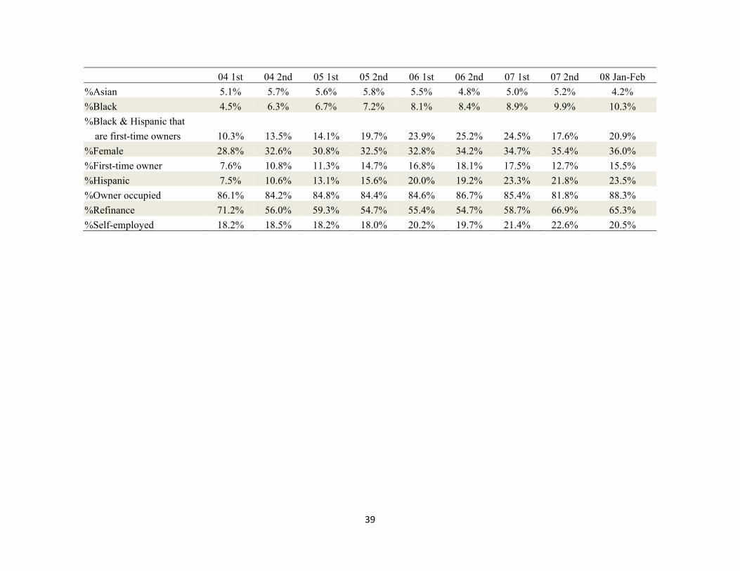
39  

04 1st 04 2nd 05 1st 05 2nd 06 1st 06 2nd 07 1st 07 2nd 08 Jan-Feb %Asian 5.1% 5.7% 5.6% 5.8% 5.5% 4.8% 5.0% 5.2% 4.2% %Black 4.5% 6.3% 6.7% 7.2% 8.1% 8.4% 8.9% 9.9% 10.3% %Black & Hispanic that are first-time owners 10.3% 13.5% 14.1% 19.7% 23.9% 25.2% 24.5% 17.6% 20.9% %Female 28.8% 32.6% 30.8% 32.5% 32.8% 34.2% 34.7% 35.4% 36.0% %First-time owner 7.6% 10.8% 11.3% 14.7% 16.8% 18.1% 17.5% 12.7% 15.5% %Hispanic 7.5% 10.6% 13.1% 15.6% 20.0% 19.2% 23.3% 21.8% 23.5% %Owner occupied 86.1% 84.2% 84.8% 84.4% 84.6% 86.7% 85.4% 81.8% 88.3% %Refinance 71.2% 56.0% 59.3% 54.7% 55.4% 54.7% 58.7% 66.9% 65.3% %Self-employed 18.2% 18.5% 18.2% 18.0% 20.2% 19.7% 21.4% 22.6% 20.5%

  

40  

Table 2. Delinquency Prediction: Probit Analysis

The dependent variable is loan delinquency, and the estimation method is probit. The definitions of all variables are given in Table 1 Panel A. Reported are the coefficients (Coef), t-statistics (t-stat) that adjust for clustering at the MSA level, and the average partial effects (APE). At the bottom of the table, we report the sample frequency of delinquency, the pseudo R-squared, the number of observations and the number of clusters (at the MSA level).

1 2 3 4 Bank/Full-Doc Bank/Low-Doc Broker/Full-Doc Broker/Low-Doc Coef t-stat APE Coef t-stat APE Ceof t-stat APE Coef t-stat APE LTV 1.693 14.61 36.15% 2.480 19.41 56.35% 2.028 17.81 50.99% 3.021 19.15 91.45% AddLTV 1.467 7.24 31.32% 1.566 7.44 35.57% 1.665 15.98 41.84% 2.975 24.28 90.05% Loan (log) 0.113 4.08 2.42% 0.178 7.23 4.04% 0.214 8.83 5.38% 0.252 8.78 7.64% SecondLien 0.245 1.78 5.22% 0.729 6.23 16.56% 0.498 8.07 12.52% 0.297 3.79 9.00% Refinance -0.046 -1.08 -0.97% -0.038 -1.32 -0.86% -0.050 -2.15 -1.25% 0.097 5.49 2.94% PrepayPenalty 0.111 2.1 2.37% 0.028 0.7 0.63% 0.005 0.26 0.12% 0.082 6.38 2.49% FirstTimeOwner -0.186 -4.2 -3.97% -0.072 -1.17 -1.63% -0.010 -0.61 -0.24% -0.054 -3.81 -1.62% OwnerOccupied -0.259 -5.31 -5.53% -0.275 -8.18 -6.24% -0.350 -13.75 -8.79% -0.281 -10.31 -8.51% OneBorrower 0.267 12.81 5.70% 0.346 15.34 7.87% 0.292 19.32 7.34% 0.298 17.07 9.03% Income (log) -0.108 -6.91 -2.30% 0.023 1.32 0.53% -0.064 -4.33 -1.61% 0.041 4.75 1.26% IncomeMiss -0.033 -0.28 -0.71% -0.006 -0.13 -0.14% -0.160 -2.97 -4.02% 0.155 6.98 4.71% CashResv -0.047 -5.61 -1.01% -0.027 -3.61 -0.60% -0.090 -17.94 -2.27% -0.069 -16.12 -2.10% CreditScore -0.009 -53.89 -0.18% -0.008 -31.84 -0.17% -0.008 -49.91 -0.21% -0.007 -71.41 -0.21% Female -0.043 -1.71 -0.93% -0.014 -0.75 -0.32% -0.003 -0.2 -0.07% 0.003 0.34 0.08% Hispanic 0.276 5.5 5.89% 0.219 3.78 4.98% 0.391 7.75 9.83% 0.275 10.55 8.33% Black 0.129 2.74 2.76% 0.156 2.75 3.55% 0.167 5.16 4.21% 0.120 4.53 3.64% Asian -0.053 -0.52 -1.13% -0.052 -1.05 -1.18% 0.022 0.69 0.55% 0.037 1.25 1.12% Age (log year) -0.089 -3.65 -1.90% 0.020 1.04 0.45% -0.020 -1.64 -0.50% 0.005 0.57 0.16% Tenure(log month) -0.018 -2.01 -0.38% -0.045 -5.25 -1.02% -0.012 -1.87 -0.30% -0.035 -6.95 -1.06% TenureMiss -0.072 -1.16 -1.54% -0.174 -4.01 -3.95% -0.251 -7.56 -6.32% -0.266 -11.52 -8.07%

  

41  

1 2 3 4 Bank/Full-Doc Bank/Low-Doc Broker/Full-Doc Broker/Low-Doc Coef t-stat APE Coef t-stat APE Ceof t-stat APE Coef t-stat APE SelfEmploy -0.001 -0.03 -0.03% 0.053 2.82 1.20% 0.051 2.44 1.29% 0.000 -0.01 0.00% 2005 0.007 0.2 0.15% 0.155 3.99 3.52% 0.026 0.9 0.65% 0.138 5.28 4.18% 2006 0.018 0.49 0.39% 0.170 4.21 3.86% 0.053 1.13 1.34% 0.265 6.3 8.03% 2007 -0.188 -3.88 -4.02% 0.108 2.14 2.46% -0.078 -1.48 -1.95% 0.167 3.85 5.05% 2008 -0.263 -4.07 -5.61% -0.039 -0.49 -0.90% -0.167 -2.8 -4.20% 0.048 0.88 1.46% Constant 2.7901 7.82 0.231 0.75 1.00 2.53 -1.51 -4.17 %Delinquency and (Pseudo) R-suqared 0.132 0.221 0.180 0.136 0.236 0.182 0.316 0.146 # obs and # clusters 31,408 807 35,553 778 166,402 963 425,181 949

  

42  

Table 3. Delinquency Prediction: Duration Analysis The dependent variable is duration between loan origination and delinquency (or censored at the end of the sample) in months, and the estimation method is a duration model with a log-logistic distribution for the accelerated time. The definitions of all variables are given in Table 1 Panel A. Reported are the coefficients (Coef), t-statistics (t-stat) that adjust for clustering at the MSA level, and changes in the median survival time for a one unit change in a covariate while holding all other covariates at their sample mean levels (∂t/∂x). At the bottom of the table, we report the gamma coefficient and its standard error, the sample mean of median survival time and its standard deviation, the number of observations, and the pseudo R-squared. The number of clusters (at the MSA level) is the same as in Panel A.

1 2 3 4 Bank/Full-Doc Bank/Low-Doc Broker/Full-Doc Broker/Low-Doc Coef t-stat ∂t/∂x Coef t-stat ∂t/∂x Ceof t-stat ∂t/∂x Coef t-stat ∂t/∂x LTV -2.730 -15.02 -804.84 -2.838 -23.39 -284.86 -2.641 -19.51 -249.19 -3.267 -34.08 -178.40 AddLTV -1.773 -5.49 -522.68 -1.516 -9.27 -152.13 -1.952 -15.67 -184.20 -2.774 -35.27 -151.45 Loan (log) -0.135 -3.31 -39.84 -0.193 -8.00 -19.33 -0.263 -9.4 -24.77 -0.237 -9.04 -12.95 SecondLien -0.683 -3.07 -149.30 -0.953 -8.02 -63.67 -0.726 -8.94 -51.86 -0.553 -8.52 -24.73 Refinance 0.092 1.41 26.53 0.032 1.04 3.16 0.098 3.49 9.23 -0.087 -5.99 -4.79 PrepayPenalty -0.149 -1.79 -41.13 0.014 0.32 1.45 0.064 2.77 6.16 -0.022 -1.98 -1.19 FirstTimeOwner 0.299 4.05 101.03 0.035 0.55 3.58 0.001 0.03 0.06 0.052 4.88 2.91 OwnerOccupied 0.338 4.83 89.73 0.262 8.32 24.87 0.430 10.51 34.62 0.302 9.58 14.87 OneBorrower -0.417 -12.2 -121.26 -0.378 -14.23 -40.34 -0.370 -24.23 -35.91 -0.299 -13.89 -17.67 Income (log) 0.165 7.21 48.78 -0.009 -0.46 -0.93 0.079 3.86 7.43 -0.040 -4.89 -2.21 IncomeMiss 0.070 0.37 21.37 0.059 1.08 6.01 0.241 3.16 25.57 -0.156 -7.37 -8.26 CashResv 0.076 5.67 22.42 0.026 3.09 2.58 0.129 16.18 12.21 0.075 13.07 4.12 CreditScore 0.015 33.81 4.35 0.009 17.82 0.89 0.012 25.22 1.14 0.007 23.77 0.39 Female 0.072 1.77 21.46 0.012 0.56 1.18 0.005 0.32 0.50 -0.001 -0.15 -0.06 Hispanic -0.393 -4.91 -98.47 -0.203 -3.65 -18.85 -0.385 -8.47 -31.83 -0.181 -10.12 -9.45 Black -0.157 -2.08 -43.22 -0.166 -3.19 -15.44 -0.229 -5.38 -19.86 -0.149 -5.42 -7.65 Asian 0.063 0.39 19.15 0.077 1.48 8.06 0.010 0.26 0.98 0.000 0.00 -0.01 Age (log year) 0.187 4.71 55.06 -0.014 -0.71 -1.43 0.039 2.53 3.66 -0.014 -1.79 -0.77

  

43  

1 2 3 4 Bank/Full-Doc Bank/Low-Doc Broker/Full-Doc Broker/Low-Doc Coef t-stat ∂t/∂x Coef t-stat ∂t/∂x Ceof t-stat ∂t/∂x Coef t-stat ∂t/∂x Tenure(log month) 0.025 1.61 7.22 0.045 5.00 4.56 0.009 1.26 0.86 0.028 6.36 1.55 TenureMiss 0.116 1.17 35.85 0.163 3.41 17.38 0.324 9.29 33.03 0.232 9.83 13.42 SelfEmploy 0.038 0.45 11.42 -0.047 -2.24 -4.70 -0.066 -2.27 -6.05 -0.008 -0.86 -0.45 2005 -0.208 -3.45 -58.24 -0.383 -9.17 -34.90 -0.190 -5.07 -17.06 -0.335 -15.5 -16.59 2006 -0.495 -8.25 -127.96 -0.694 -17.66 -61.72 -0.486 -8.4 -41.77 -0.750 -22.47 -38.71 2007 -0.660 -8.28 -170.11 -1.058 -20.27 -91.32 -0.743 -9.98 -64.47 -1.031 -27.05 -50.05 2008 -0.850 -8.76 -173.24 -1.350 -14.5 -75.94 -0.943 -11.44 -58.94 -1.400 -25.28 -41.57 Constant -1.905 -3.02 3.284 8.35 1.430 2.51 5.192 15.61 Gamma and std. err 0.866 0.021 0.614 0.021 0.747 0.018 0.577 0.021 Median time (months) 300.1 100.4 94.4 54.6 #obs and (Pseudo) R-squared 31,400 0.174 35,550 0.141 166,399 0.162 425,180 0.145

  

44  

Table 4. Choice of Loan Origination Channel and Documentation Level

Panel A: Without neighborhood information The dependent variable is the choice of broker channel, that of low documentation, and that of the combination of two. The estimation method is probit. The definitions of all variables are given in Table 1 Panel A. Reported are the coefficients (Coef), t-statistics (t-stat) that adjust for clustering at the MSA level, and the average partial effects. At the bottom of the table, we report the average of the dependent variables (the sample frequency of the choices), and the pseudo R-squared.

1 2 3 Dep. Var. Broker Low-Doc Broker Issue/Low Doc Coef t-stat APE Coef t-stat APE Coef t-stat APE LTV 0.372 5.14 5.67% -0.773 -6.82 -19.68% -0.506 -5.18 -14.91%AddLTV 3.730 14.92 56.90% 0.411 3.31 10.48% 1.088 8.17 32.09%Loan (log) 0.088 3.02 1.34% 0.220 11.46 5.61% 0.171 7.69 5.04% SecondLien -1.896 -10.84 -28.92% -0.160 -2.17 -4.06% -0.497 -5.92 -14.67%Refinance -0.146 -5.26 -2.23% -0.053 -2.2 -1.35% -0.092 -5.26 -2.72%FirstTimeOwner 0.331 16.21 5.05% -0.047 -2.71 -1.19% -0.004 -0.26 -0.12%OwnerOccupied 0.126 3.25 1.92% -0.047 -3.07 -1.20% 0.082 3.1 2.42% OneBorrower 0.217 18.38 3.31% 0.507 37.65 12.92% 0.449 39.55 13.24%Income (log) -0.038 -3.49 -0.57% 0.241 15.01 6.14% 0.218 12.55 6.43% IncomeMiss 0.128 3.28 1.95% 2.270 56.13 57.80% 1.606 34.22 47.36%CashResv -0.015 -1.84 -0.23% 0.003 0.88 0.07% -0.003 -0.85 -0.09%CreditScore -0.001 -14.22 -0.02% 0.002 13.93 0.05% 0.001 9.10 0.03% Female 0.027 3.67 0.41% 0.150 11.1 3.82% 0.125 10.61 3.70% Hispanic 0.448 13.53 6.84% 0.432 6.67 11.00% 0.475 8.66 14.02%Black 0.439 15.57 6.70% -0.030 -1.15 -0.77% 0.059 2.14 1.75% Asian 0.485 18.38 7.41% 0.368 18.51 9.37% 0.443 25.73 13.06%Age (log year) -0.039 -3.72 -0.59% 0.001 0.06 0.01% -0.013 -1.87 -0.39%Tenure(log month) -0.017 -4.55 -0.26% -0.055 -9.6 -1.40% -0.055 -9.53 -1.62%TenureMiss 0.540 13.61 8.24% -0.350 -9.66 -8.92% -0.176 -4.8 -5.18%SelfEmploy 0.208 8.8 3.18% 1.036 48.57 26.38% 0.775 27.6 22.85%2005 0.339 12.98 5.18% 0.261 14.42 6.65% 0.306 16.99 9.01% 2006 0.443 12.73 6.77% 0.542 30.15 13.81% 0.544 26.01 16.05%2007 0.419 17.44 6.40% 0.263 16 6.70% 0.318 15.55 9.38% 2008 0.196 5.3 2.99% -0.329 -12.57 -8.38% -0.234 -7.63 -6.89%Constant 0.188 0.57 -4.213 -18.4 -3.577 -15.06 E(Dependent Variable) 0.898 0.700 0.646 #obs and (Pseudo) R-squared 658,544 0.149 658,544 0.265 658,544 0.201

  

45  

Panel B: With neighborhood information This table is identical to that in Panel A, with the addition of neighborhood covariates at the census tract or zip-code level. The definitions of all variables are given in Table 1 Panel A. For the economy of space and to avoid repetition, only results regarding the neighborhood variables are reported.

1 2 3 Dep. Var. Broker Low-Doc Broker Issue/Low Doc Coef t-stat APE Coef t-stat APE Coef t-stat APE Population(log) -0.006 -0.98 -0.10% 0.005 0.91 0.12% -0.001 -0.14 -0.02%Pctblack -0.079 -4.69 -1.23% 0.055 2.97 1.39% 0.027 1.38 0.80%Pcthisp -0.055 -1.65 -0.86% 0.175 8.88 4.46% 0.143 6.41 4.22%Medage -0.002 -3.18 -0.03% -0.001 -2.67 -0.03% -0.002 -3.19 -0.04%Avgincome 0.000 -0.51 0.00% 0.000 0.46 0.00% 0.000 0.66 0.00%Unemprate -0.001 -0.29 -0.01% -0.006 -2.19 -0.15% -0.007 -2.44 -0.19%Other controls included? Y Y Y E(Dep Var) 89.9% 69.9% 64.6% #obs and (Pseudo) R-squared 491,816 0.116 491,816 0.268 491,816 0.200

  

46  

Table 5. Non-Linear Blinder-Oaxaca Decomposition of Differences in Delinquency Rates

This table reports the non-linear Blinder-Oaxaca (1973) decomposition to the probit model. The total difference in delinquency rates between two subsamples is decomposed into an “endowment effect” and a “coefficient effect” using equations (8) (using the high average outcome subsample as the base) and (9) (using the low average outcome subsample as the base).

Panel A: Comparison of Full-Doc and Low-Doc subsamples Bank Broker Difference t-stat Percentage Difference t-stat Percentage Low-Doc sample as benchmark

Endowment Effect -0.06% -0.10 -1.20% -0.89% -1.62 -11.10%Coefficient Effect 4.87% 9.13 101.20% 8.91% 12.84 111.10%

Full-Doc sample as benchmark Endowment Effect -2.10% -2.37 -43.71% -2.84% -4.15 -35.47%Coefficient Effect 6.91% 8.12 143.71% 10.86% 12.94 135.47% Total Difference 4.81% 5.37 100% 8.02% 8.05 100%

Panel B: Comparison of Bank and Broker subsamples

Full-Doc Low-Doc Difference t-stat Percentage Difference t-stat PercentageBroker sample as benchmark

Endowment Effect 7.84% 8.09 75.69% 10.40% 12.16 76.67%Coefficient Effect 2.52% 9.46 24.31% 3.16% 8.76 23.33%

Bank sample as benchmark Endowment Effect 6.12% 10.28 59.06% 6.93% 9.88 51.10%Coefficient Effect 4.24% 5.74 40.94% 6.63% 9.45 48.90% Total Difference 10.35% 10.51 100% 13.56% 13.99 100%

  

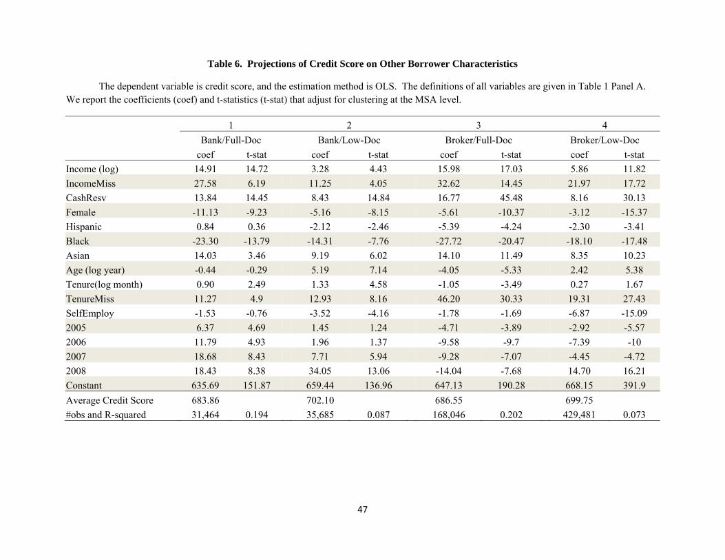
47  

Table 6. Projections of Credit Score on Other Borrower Characteristics

The dependent variable is credit score, and the estimation method is OLS. The definitions of all variables are given in Table 1 Panel A. We report the coefficients (coef) and t-statistics (t-stat) that adjust for clustering at the MSA level.

1 2 3 4 Bank/Full-Doc Bank/Low-Doc Broker/Full-Doc Broker/Low-Doc coef t-stat coef t-stat coef t-stat coef t-stat Income (log) 14.91 14.72 3.28 4.43 15.98 17.03 5.86 11.82 IncomeMiss 27.58 6.19 11.25 4.05 32.62 14.45 21.97 17.72 CashResv 13.84 14.45 8.43 14.84 16.77 45.48 8.16 30.13 Female -11.13 -9.23 -5.16 -8.15 -5.61 -10.37 -3.12 -15.37 Hispanic 0.84 0.36 -2.12 -2.46 -5.39 -4.24 -2.30 -3.41 Black -23.30 -13.79 -14.31 -7.76 -27.72 -20.47 -18.10 -17.48 Asian 14.03 3.46 9.19 6.02 14.10 11.49 8.35 10.23 Age (log year) -0.44 -0.29 5.19 7.14 -4.05 -5.33 2.42 5.38 Tenure(log month) 0.90 2.49 1.33 4.58 -1.05 -3.49 0.27 1.67 TenureMiss 11.27 4.9 12.93 8.16 46.20 30.33 19.31 27.43 SelfEmploy -1.53 -0.76 -3.52 -4.16 -1.78 -1.69 -6.87 -15.09 2005 6.37 4.69 1.45 1.24 -4.71 -3.89 -2.92 -5.57 2006 11.79 4.93 1.96 1.37 -9.58 -9.7 -7.39 -10 2007 18.68 8.43 7.71 5.94 -9.28 -7.07 -4.45 -4.72 2008 18.43 8.38 34.05 13.06 -14.04 -7.68 14.70 16.21 Constant 635.69 151.87 659.44 136.96 647.13 190.28 668.15 391.9 Average Credit Score 683.86 702.10 686.55 699.75 #obs and R-squared 31,464 0.194 35,685 0.087 168,046 0.202 429,481 0.073

  

48  

Table 7. Delinquency Analysis: Correspondent and Non-Correspondent Brokers This table repeats the analysis in Table 2 using loans originated by brokers only, where the Broker channel is decomposed into Correspondent and Non-Correspondent channels.

1 2 3 4 Correspondent/Full Doc Correspondent/Low Doc Non-Correspondent/Full Doc Non-Correspondent/Low Doc Coef t-stat APE Coef t-stat APE Ceof t-stat APE Coef t-stat APE LTV 2.035 14.57 45.51% 3.154 16.05 90.78% 2.000 17.35 51.12% 2.973 20.65 91.02% AddLTV 1.781 8.18 39.84% 3.260 18.82 93.82% 1.707 16.98 43.62% 2.929 25.83 89.66% Loan (log) 0.140 3.3 3.13% 0.264 6.45 7.61% 0.232 9.22 5.94% 0.255 9.15 7.81% SecondLien 0.278 2.05 6.22% 0.220 2.31 6.33% 0.490 7.65 12.53% 0.301 3.74 9.23% Refinance 0.012 0.31 0.26% 0.128 3.72 3.69% -0.062 -2.55 -1.57% 0.087 5.41 2.66% PrepayPenalty 0.059 1.37 1.31% 0.068 2.99 1.95% -0.015 -0.76 -0.38% 0.076 5.52 2.34% FirstTimeOwner -0.120 -3.86 -2.69% -0.098 -4.12 -2.83% 0.003 0.18 0.07% -0.048 -3.68 -1.47% OwnerOccupied -0.366 -8.23 -8.20% -0.226 -5.64 -6.51% -0.348 -13.17 -8.90% -0.288 -10.89 -8.82% OneBorrower 0.211 8.38 4.73% 0.281 14.01 8.08% 0.299 20.29 7.65% 0.300 17.5 9.18% Income (log) -0.059 -2.21 -1.32% 0.020 1.02 0.57% -0.065 -4.04 -1.67% 0.043 5.24 1.32% IncomeMiss -0.042 -0.22 -0.94% 0.053 1.14 1.52% -0.166 -2.91 -4.24% 0.174 7.8 5.32% CashResv -0.095 -8.92 -2.13% -0.096 -14.94 -2.75% -0.087 -17.22 -2.23% -0.063 -13.39 -1.92% CreditScore -0.008 -31.1 -0.19% -0.007 -50.26 -0.20% -0.008 -45.74 -0.21% -0.007 -66.9 -0.21% Female 0.015 0.56 0.33% 0.014 1.15 0.41% -0.007 -0.47 -0.18% -0.001 -0.07 -0.02% Hispanic 0.323 10.01 7.24% 0.360 10.93 10.36% 0.379 7.6 9.69% 0.254 10.11 7.76% Black 0.152 3.99 3.40% 0.103 3.63 2.98% 0.167 5.19 4.26% 0.127 4.79 3.88% Asian 0.075 1.49 1.67% 0.143 4.39 4.11% 0.010 0.29 0.25% 0.012 0.42 0.38% Age (log year) -0.021 -0.7 -0.47% 0.028 2.23 0.82% -0.019 -1.58 -0.48% 0.004 0.42 0.12% Tenure(log month) 0.007 0.74 0.15% -0.015 -2.03 -0.44% -0.018 -2.3 -0.45% -0.041 -8.77 -1.24% TenureMiss -0.009 -0.15 -0.19% -0.129 -4.13 -3.72% -0.307 -7.87 -7.84% -0.302 -11.95 -9.24% SelfEmploy 0.033 0.62 0.74% 0.022 1.06 0.63% 0.057 2.51 1.45% -0.001 -0.09 -0.03% 2005 0.049 0.97 1.11% 0.154 4.53 4.43% 0.028 0.92 0.71% 0.137 5.31 4.20% 2006 0.031 0.57 0.68% 0.247 5.7 7.10% 0.067 1.34 1.72% 0.271 6.29 8.30% 2007 -0.071 -1.17 -1.58% 0.161 3.28 4.63% -0.082 -1.54 -2.10% 0.166 3.86 5.07%

  

49  

1 2 3 4 Correspondent/Full Doc Correspondent/Low Doc Non-Correspondent/Full Doc Non-Correspondent/Low Doc Coef t-stat APE Coef t-stat APE Ceof t-stat APE Coef t-stat APE 2008 -0.153 -0.97 -3.42% -0.094 -0.63 -2.70% -0.189 -3.15 -4.83% 0.037 0.69 1.13% Constant 1.706 3.02 -1.888 -4.44 0.83 1.99 -1.484 -3.93 %Delinquency and (Pseudo) R-squared 0.189 0.171 0.180 0.161 0.246 0.184 0.331 0.143 # obs and # clusters 25,666 657 88,778 672 140,736 955 336,403 936

  

50  

Table 8. Out-of-Sample Model Predictive Power: Across Loan Types and Over Time

This Table reports the “excess percentage of correct predictions” as defined in equation (10). We reporte percentage of delinquent loans correctly predicted (S1), percentage of non-delinquent loans correctly predicted (S2), and the total percentage of correct predictions in excess of 50% (S). Each measure is reported for the full sample, and separately for the four sub-samples, and is reported by semi-annual intervals, together with the all-sample average.

05 1st half 05 2nd half 06 1st half 06 2nd half 07 1st half 07 2nd half

& 08 Jan-FebAll-TimeAverage

% Delinquency correctly predicted (S1) 54.2% 54.4% 52.2% 42.5% 52.9% 46.1% 50.4% Bank/Full-Doc 57.6% 46.6% 43.3% 46.7% 40.9% 50.1% 47.5% Bank/Low-Doc 51.9% 43.3% 42.5% 48.3% 51.4% 44.0% 46.9% Broker/Full-Doc 61.6% 67.3% 58.9% 56.6% 66.9% 54.2% 60.9% Broker/Low-Doc 50.7% 51.0% 51.4% 39.7% 50.4% 41.5% 47.4%% Non-Delinquency correctly predicted (S2) 76.3% 73.9% 71.9% 76.9% 75.7% 78.9% 75.6% Bank/Full-Doc 87.1% 89.5% 87.3% 86.5% 88.0% 83.2% 86.9% Bank/Low-Doc 75.4% 76.2% 76.8% 74.3% 74.8% 79.5% 76.2% Broker/Full-Doc 80.6% 74.1% 73.9% 76.5% 74.1% 72.9% 75.4% Broker/Low-Doc 72.7% 71.9% 69.7% 76.6% 75.6% 82.0% 74.7%Total Excess % of correct prediction (S) 15.3% 14.2% 12.1% 9.7% 14.3% 12.5% 13.0% Bank/Full-Doc 22.4% 18.0% 15.3% 16.6% 14.4% 16.7% 17.2% Bank/Low-Doc 13.7% 9.8% 9.6% 11.3% 13.1% 11.7% 11.5% Broker/Full-Doc 21.1% 20.7% 16.4% 16.6% 20.5% 13.6% 18.1% Broker/Low-Doc 11.7% 11.5% 10.5% 8.1% 13.0% 11.8% 11.1%

  

51  

Table 9. Interest Rates, Loan Types, and Delinquency Rates

This table examines the determinants of interest rates (expressed in percentage points), with loan types as the main regressors of interest. Odd columns apply the linear regression on the initial and current interest rates; even columns use the probit model on the occurrence of delinquency (reported are the average marginal probabilities). The sample for columns (1) and (2) include all fixed-rate loans; that for columns (3) and (4) include all variable-rate loans that have already incurred an interest rate change by 2008; and that for columns (5) and (6) include all fixed-rate loans issued after July 1st, 2007. The t-statistics reported in the brackets adjust for heteroskedasticity and clustering at the MSA level.

(1) (2) (3) (4) (5) (6) Dependent Variables InitialRate Delinq CurrentRate Delinq InitialRate Delinq Bank/Low-Doc 0.2973 0.0440 -0.0844 0.0741 0.2308 0.0640 [17.00] [5.40] [-2.21] [5.49] [11.73] [3.37] Broker/Full-Doc 0.0591 0.0127 -0.7693 0.0245 0.0985 0.0511 [3.08] [2.67] [-18.11] [1.94] [7.21] [5.76] Broker/Low-Doc 0.2883 0.0861 -0.6937 0.1053 0.4188 0.0841 [13.22] [14.90] [-17.01] [9.69] [18.25] [8.20] LTV 1.2590 0.5430 1.0516 0.8601 1.3416 0.5065 [29.64] [17.31] [17.11] [15.54] [31.77] [17.60] AddLTV 0.6591 0.5572 0.2416 0.9035 0.2153 0.3128 [7.98] [17.48] [2.00] [16.23] [1.77] [6.26] Loan (log) -0.2405 0.0700 -0.3001 0.1004 -0.3471 0.0869 [-18.63] [10.61] [-22.68] [10.70] [-24.68] [9.18] SecondLien 3.1051 -0.0077 * * 2.2254 0.3143 [30.01] [-0.50] [22.12] [5.92] Refinance -0.2726 0.0175 -0.1027 0.0339 -0.1326 0.0211 [-18.51] [4.29] [-4.55] [4.39] [-8.00] [3.34] PrepayPenalty -0.2232 0.0249 -0.2522 -0.0126 0.2174 0.0586 [-17.12] [4.66] [-9.78] [-2.44] [4.32] [1.97] FirstTimeOwner 0.0376 -0.0097 0.1572 -0.0191 -0.0871 0.0069 [3.55] [-2.56] [7.22] [-2.96] [-5.16] [1.04] OwnerOccupied -0.5418 -0.0579 -0.6281 -0.0665 -0.3944 -0.0458 [-23.90] [-9.36] [-22.63] [-7.18] [-17.30] [-4.30] OneBorrower 0.0688 0.0733 -0.0067 0.0956 0.0369 0.0742 [10.23] [19.96] [-1.22] [19.30] [4.28] [12.47]

  

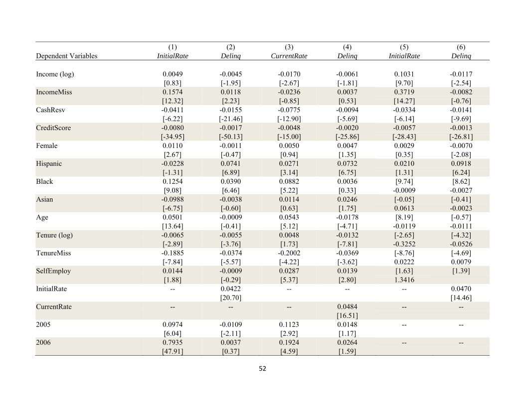
52  

(1) (2) (3) (4) (5) (6) Dependent Variables InitialRate Delinq CurrentRate Delinq InitialRate Delinq Income (log) 0.0049 -0.0045 -0.0170 -0.0061 0.1031 -0.0117 [0.83] [-1.95] [-2.67] [-1.81] [9.70] [-2.54] IncomeMiss 0.1574 0.0118 -0.0236 0.0037 0.3719 -0.0082 [12.32] [2.23] [-0.85] [0.53] [14.27] [-0.76] CashResv -0.0411 -0.0155 -0.0775 -0.0094 -0.0334 -0.0141 [-6.22] [-21.46] [-12.90] [-5.69] [-6.14] [-9.69] CreditScore -0.0080 -0.0017 -0.0048 -0.0020 -0.0057 -0.0013 [-34.95] [-50.13] [-15.00] [-25.86] [-28.43] [-26.81] Female 0.0110 -0.0011 0.0050 0.0047 0.0029 -0.0070 [2.67] [-0.47] [0.94] [1.35] [0.35] [-2.08] Hispanic -0.0228 0.0741 0.0271 0.0732 0.0210 0.0918 [-1.31] [6.89] [3.14] [6.75] [1.31] [6.24] Black 0.1254 0.0390 0.0882 0.0036 [9.74] [8.62] [9.08] [6.46] [5.22] [0.33] -0.0009 -0.0027 Asian -0.0988 -0.0038 0.0114 0.0246 [-0.05] [-0.41] [-6.75] [-0.60] [0.63] [1.75] 0.0613 -0.0023 Age 0.0501 -0.0009 0.0543 -0.0178 [8.19] [-0.57] [13.64] [-0.41] [5.12] [-4.71] -0.0119 -0.0111 Tenure (log) -0.0065 -0.0055 0.0048 -0.0132 [-2.65] [-4.32] [-2.89] [-3.76] [1.73] [-7.81] -0.3252 -0.0526 TenureMiss -0.1885 -0.0374 -0.2002 -0.0369 [-8.76] [-4.69] [-7.84] [-5.57] [-4.22] [-3.62] 0.0222 0.0079 SelfEmploy 0.0144 -0.0009 0.0287 0.0139 [1.63] [1.39] [1.88] [-0.29] [5.37] [2.80] 1.3416 InitialRate -- 0.0422 -- -- -- 0.0470 [20.70] [14.46] CurrentRate -- -- -- 0.0484 -- -- [16.51] 2005 0.0974 -0.0109 0.1123 0.0148 -- -- [6.04] [-2.11] [2.92] [1.17] 2006 0.7935 0.0037 0.1924 0.0264 -- -- [47.91] [0.37] [4.59] [1.59]

  

53  

(1) (2) (3) (4) (5) (6) Dependent Variables InitialRate Delinq CurrentRate Delinq InitialRate Delinq 2007 0.6725 -0.0277 0.3222 -0.0099 -- -- [62.31] [-2.93] [7.17] [-0.55] 2008 0.6183 -0.0293 * * -0.1945 -0.0048 [37.10] [-2.72] [-19.77] [-1.03] Constant 14.2234 15.7684 14.2567 [67.95] [49.11] [47.66] Observations 310,785 310,785 107,125 107,125 52,878 52,878 R-squared 0.766 0.427 0.438 *: The variable drops out due to a lack of variation in the subsample.