Skeena Sockeye In-river Run Reconstruction Analysis Model

and

Preliminary Analysis Results for 1982-2009

Prepared by

Karl K. English, Cameron Noble and Anita Blakley

LGL Limited

environmental research associates 9768 Second Street,

Sidney, BC V8L 3Y8

with substantial assistance from

William J. Gazey and Steve Cox-Rogers

for

Pacific Salmon Foundation

15 October 2012

i

TABLE OF CONTENTS

1.0 INTRODUCTION ............................................................................................................... 1 1.1 Analysis Objectives.......................................................................................................... 1

2.0 DATA SOURCES AND PREPARATION ......................................................................... 1

2.1 Sockeye Stocks and Stock Aggregates............................................................................. 1 2.2 Fishery Definitions........................................................................................................... 2 2.3 Escapement....................................................................................................................... 2 2.4 Run Timing ...................................................................................................................... 2 2.5 Fishery Residence Time................................................................................................... 3 2.6 Catch................................................................................................................................. 3

2.7 Fishing Patterns ................................................................................................................ 4 3.0 RUN RECONSTRUCTION MODEL................................................................................. 4

3.1 Model Assumptions.......................................................................................................... 4 3.2 Model Structure................................................................................................................ 5

4.0 PRELIMINARY RESULTS................................................................................................ 6 5.0 NEXT STEPS ...................................................................................................................... 7

1

1.0 INTRODUCTION The Fraser, Skeena and Nass watersheds are the three largest sockeye producing watersheds in British Columbia. Exploitation rate estimates for the Nass and Skeena Sockeye stock aggregates are estimated annually using the Northern Boundary Sockeye Run Reconstruction (NBSRR) Model (English et al. 2004b; 2005; Alexander et al. 2010). English et al. (2011) provided estimates of marine exploitation rates for each Nass and Skeena sockeye Conservation Unit (CU) using estimates of the migration timing for each CU. These analyses have not included the details on the location and timing of in-river fisheries needed to estimate harvests for the various sockeye CUs or sub-stocks within each watershed. In some years, in-river harvest account for a large portion of the Canadian harvest of sockeye returning to these rivers. Run reconstruction analyses have been used to estimate CU specific harvest rates for in-river fisheries targeting Fraser sockeye and Chinook salmon (English et al. 2007; Noble 2011). This report provides a brief outline of a Skeena Sockeye In-River (SSIR) run reconstruction model built to combine information on run timing and escapements for Skeena sockeye sub-stocks with catch estimates for each sockeye fishery within the Skeena watershed. The model is similar to those developed for the Fraser River sockeye fisheries within the Fraser watershed except that the Skeena model moves fish forward (upstream) through the fisheries and subtracts sockeye catches from estimates of the number of sockeye entering the Skeena River each day. The Fraser sockeye reconstructs the run entering the Fraser River by adding catches to daily estimates of escapement for each sub-stock. 1.1 Analysis Objectives Estimates of in-river harvest by sub-stock are needed to be combined with those for marine fisheries to estimate total exploitation rates for Skeena sockeye. The SSIR model provides a systematic process for combining information on catch, fishery timing, stock specific migration rates through fisheries, escapement and river entry run timing by sub-stock. The results from these run reconstruction analyses will be combined with the marine harvest rates from NBSRR model to provide estimates of the total exploitation rate for each Skeena sockeye sub-stock and the biological basis for the forward looking model needed to evaluate alternative fisheries and fisheries management options for Skeena sockeye sub-stocks. 2.0 DATA SOURCES AND PREPARATION 2.1 Sockeye Stocks and Stock Aggregates The model has the capacity to accommodate details for as many sockeye sub-stocks or run-timing groups as can be defined using the available data and combine these stocks into any number of management groups. Initial analyses of available run-timing data resulted in the definition of 20 sub-stocks for the Skeena watershed (English et al. 2011).

2

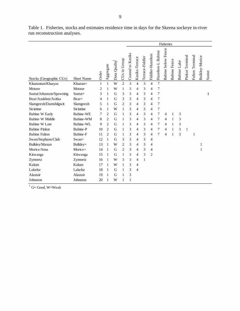
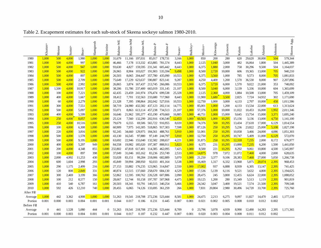
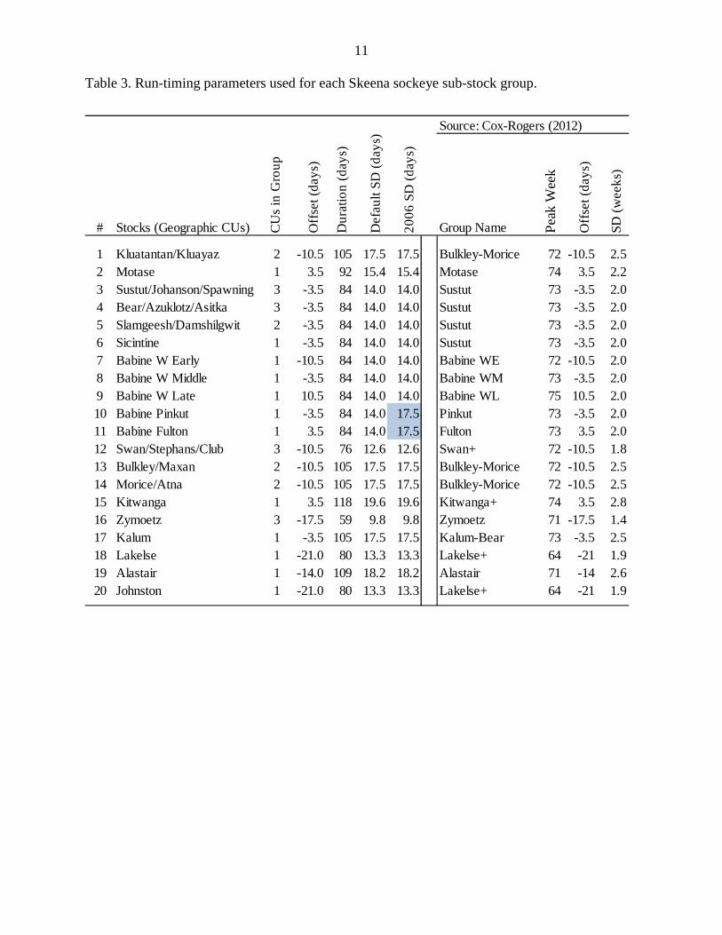
2.2 Fishery Definitions The SSIR model includes two types of fisheries (FSC and ESSR) and 12 fishing areas: 3 Tsimshian fishery strata in the lower Skeena and 9 fishing areas used by other Skeena First Nations above Fiddler Creek (Table 1). All of the fisheries on the Skeena River (mainstem) harvest multiple stocks and stock composition estimates are not available for these fisheries. Consequently, run reconstruction analysis is required to distribute the reported weekly catches between the stocks vulnerable to each fishery. Some FSC and most ESSR fisheries occur in locations where only a single stock is affected. The harvest rate estimates for these fisheries were computed by dividing the catch by the sum of the annual catch and escapement for these stocks. 2.3 Escapement and Entering Run Size Annual escapement estimates for each Skeena sockeye CU were combined with daily Tyee test fishery data and stock-specific run timing parameters to produce estimates of daily escapement past the Tyee test fishery for each CU. Annual estimates of spawning escapement for the 20 Skeena CU-run timing groups were derived from three sources: 1) nuSEDS data for 11 non-Babine sockeye CUs; 2) DFO Prince Rupert historical databases for the 5 Babine sockeye stock groups; and 3) assumed fixed values for the remaining 4 non-Babine sockeye CUs without escapement monitoring programs. Each of the non-Babine sockeye stocks had one or more years of missing escapement estimates and these were filled in by using the average of the estimates for adjacent years or interpolating between the available estimates. The filled in values are highlighted in yellow in Table 2. The annual escapement estimates for sub-stocks with terminal fisheries (i.e. Pinkut, Fulton, Sustut and Bulkley-Morice) were increased to account for catches in these terminal fisheries prior to determining the portions that each sub-stock proportions represents of the total return of Skeena sockeye in a given year. These sub-stock proportions were combined with annual estimates of the total sockeye abundance passing Tyee and run-timing parameters derived from analysis of 2000-10 Tyee DNA samples (Cox-Rogers, DFO Rupert, pers. comm.) to compute the daily abundance passing Tyee for each sub-stock. 2.4 Run Timing Estimates of river entry timing for 20 sub-stocks of Skeena sockeye were obtained from information reported in a memorandum entitled “SKEENA SOCKEYE SUB-STOCK RUN-TIMING AND ABUNDANCE EVALUATED USING TYEE TEST FISHERY DNA: 2000-2010” prepared by Steve Cox-Rogers dated 23 February 2012. The relative timing for each sub-stock was used to determine the offset difference between the average annual timing for all Skeena sockeye and that for a specific sub-stock. For example: Lakelse sockeye were estimated to have a timing 3 weeks earlier than the median timing for Skeena sockeye, therefore, the offset parameter was set at -21 days for Lakelse sockeye. The duration of the run for each sub-stock was also derived from the 2000-2010 DNA stock composition estimates. The parameter used to define the duration was the standard deviation (SD) measured in number of days. Table 3 provides the offset and SD parameters for each sub-stock. The run timing curve for each sub-stock was defined by a normal curve where the mid-point was defined by combining the stock-specific offset with the median date of sockeye migration past the Tyee test fishery and the start

3

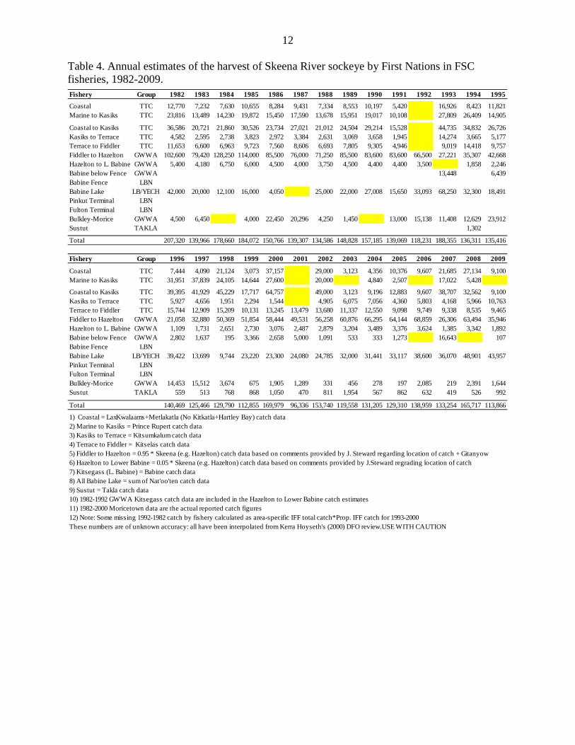
and end points for each timing curve were 3 SD units each side of the mid-point. Therefore, the SD of 13.3 d for Lakelse sockeye results in a total duration of 80 days for this stock. For our initial analysis we used the same offset and SD parameters for each year except 2006, when the duration of the run (SD) for the two large enhanced stocks (Pinkut and Fulton) was increased from 14 to 17.5 days (total duration increased from 84 to 105 days) in order to reflect the notably longer duration of the Skeena sockeye run observed in 2006. 2.5 Fishery Residence Time Residency time was defined as the number of days (to the nearest day) a stock resides within the boundaries of a single fishery. These residence times were derived from historical tagging studies, the differences between peak abundances estimated at Tyee and the Babine fence, and information on the size (river kms) and location of each fishery (English et al 1985, Steve Cox-Rogers, pers. comm.). 2.6 Catch Estimates of annual harvest by Skeena River First Nations for each fishery location and type from 1982-2009 were obtained from DFO records (Table 4, Steve Cox-Rogers, pers. comm.). Estimates of the annual harvests were available for most FSC fisheries from 1996-2009. FSC catch estimates were not available for two FSC fisheries (Kitsegass and Sustut) prior to 1993 and there were notable missing estimates for a large portion of the Tsimshian fisheries in 1992 and 2001, Lake Babine FN fisheries in 1987 and the Bulkley River (Wet’suwet’en) fisheries in 1984 and 1990. ESSR commercial fisheries were first conducted on the Skeen River in 1993. These fisheries are only permitted at specific locations within the Skeena watershed when managers determine that Escapements Surplus to Spawning Requirements (ESSR) can be harvested for some Skeena sockeye stocks. In recent years, additional commercial fishing opportunities have been provided to Skeena River First Nations through the transfer of sockeye allocations for Area 4 seine and gillnet licences to in-land “demonstration” fisheries. From 1993-2009, there have been 10 years when ESSR and/or demonstration fisheries have been conducted within the Skeena watershed and total harvests in these fisheries have ranged from 13,700 to over 780,000 sockeye (Table 5). The breakdown of these annual harvest estimates to weekly harvests was not available for the analyses conducted to date (15 October 2012), so the available annual harvest estimates were prorated to weekly harvest estimates using the year specific estimates of the number of sockeye passing Tyee each week adjusted for the time required for sockeye to migrate from Tyee to each fishery. Ideally, these initial estimates of weekly catch will be replaced with the best available estimates from Skeena First Nations. If weekly estimates are not available of some in-river fisheries, additional information on the timing and duration of these fisheries could be used to improve the estimate of weekly catches. Adjustments to the timing of FSC harvests are not expected to have a significant impact on the harvest rate estimates because of the small relative magnitude and protracted nature of these fisheries. The timing of the more substantial ESSR fisheries along the Skeena mainstem from Fiddler Creek to the Babine fence could have a significant impact on harvest rates for sockeye stocks migrating through these fisheries.

4

2.7 Fishing Patterns Detailed information on fishing patterns (number of fishing days per week) for Skeena First Nation fisheries have not been obtained so the SSIR model currently runs on the assumption that weekly First Nation catches are distributed equally across all days in a week. 3.0 RUN RECONSTRUCTION MODEL The theoretical basis of run reconstruction analysis for salmon stocks and fisheries are described in Starr and Hilborn (1988), Gazey et al. (1989), Cave and Gazey (1994), Gazey and English (2000) and English et al. (2007). The proposed analytical model will use essentially the same algorithms as those described in our 2007 PSARC approved report for Fraser Chinook (English et al. 2007). The sequential steps in the run reconstruction are described below:

1. read all catch, escapement, run-timing parameters and total daily abundance estimates derived from Tyee test fishery data;

2. estimate the daily escapement past the Tyee test fishery for each sub-stock;

3. starting with the first fishery in the lower Skeena, assign portions of the weekly

catch to each sub-stock present in the fishery using the estimated constant daily harvest rate for all days in a week based on the assumption of equal vulnerability for all sub-stocks present during the week;

4. subtract the catch for each stock from the abundance of that stock that entered the

fishery; 5. repeat steps 3 and 4 for each fishery moving upstream along the Skeena mainstem

and into the tributaries; 6. total the catch and escapement estimates for each sub-stock and calculate annual

estimates for the in-river harvest rates for each sockeye sub-stock and management group.

The model control worksheet has locations where the user can define the start and end years for the analysis and input files to be used for the run reconstruction analyses.

A more mathematically rigorous description of the above methods can be found in English et al. (2007). 3.1 Model Assumptions The assumptions associated with the SSIR run reconstruction analyses model include:

a. The sockeye sub-stocks included in the models adequately represent the run timing and total escapement for Skeena sockeye;

5

b. The daily sockeye CPUE estimates from Tyee test fishery provides a reliable indication of the relative abundance sockeye entering the Skeena River;

c. The escapement estimates and run-timing parameters available for Skeena sub-stocks can be used with the assumption of normal distributions for each stock to derive daily stock composition estimates for the run at Tyee;

d. The fisheries and catch data included in the model adequately represent the timing and location of fisheries that harvest sockeye within the Skeena watershed; and

e. All stocks are equally vulnerable to harvesting when present in a fishery, such that harvests of a stock are proportional to the relative abundance of that stock in that fishery during the fishing period.

3.2 Model Structure In order to expedite these run reconstruction analyses, we have used a model structure that is very similar to that used for the Fraser Chinook run reconstruction model (i.e. a MS Excel model prepared using the Visual Basic programming language). The model contains a series of sub-routines and function calls to read input data from MS Excel worksheets, conduct the analyses and output results to MS Excel files. The model includes the following sub-routines and functions: Sub Reconstruction() - main program where public variables are defined and all other sub-routines are called. Sub Init() – prompts for input from the user, opens the input files, creates the output files and writes the initial column headings into each output file. Sub FishResSpawn() – reads the fishery residence times for each stock and determines the cumulative number of days between each fishery and the escapement area for each stock. Sub Calc_Escape() – calculates the daily escapement for each stock for a specific year. Sub Reconstruct() - conducts the run reconstruction analysis working backward through the fisheries building on the daily escapement estimates. Function CalcHarvestRate() - calculates the weekly harvest rate for a given fishery based on the size of the reported catch, number of fishing days per week and the number of sockeye that escaped from that fishery. Function gs() – calculates the weekly catch for a given harvest rate. This function is used in the bisection algorithm to determine the weekly harvest rate that would result in the reported catch. Sub-OutputData() – writes the run reconstruction results to the various output files.

6

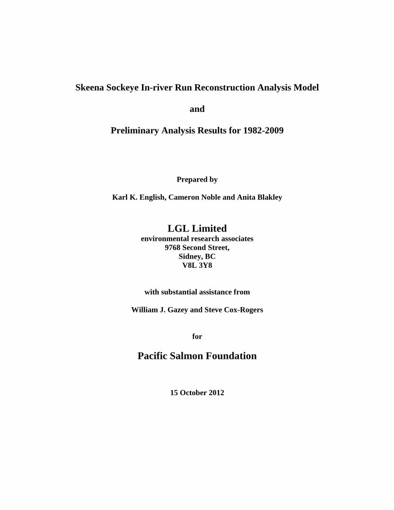
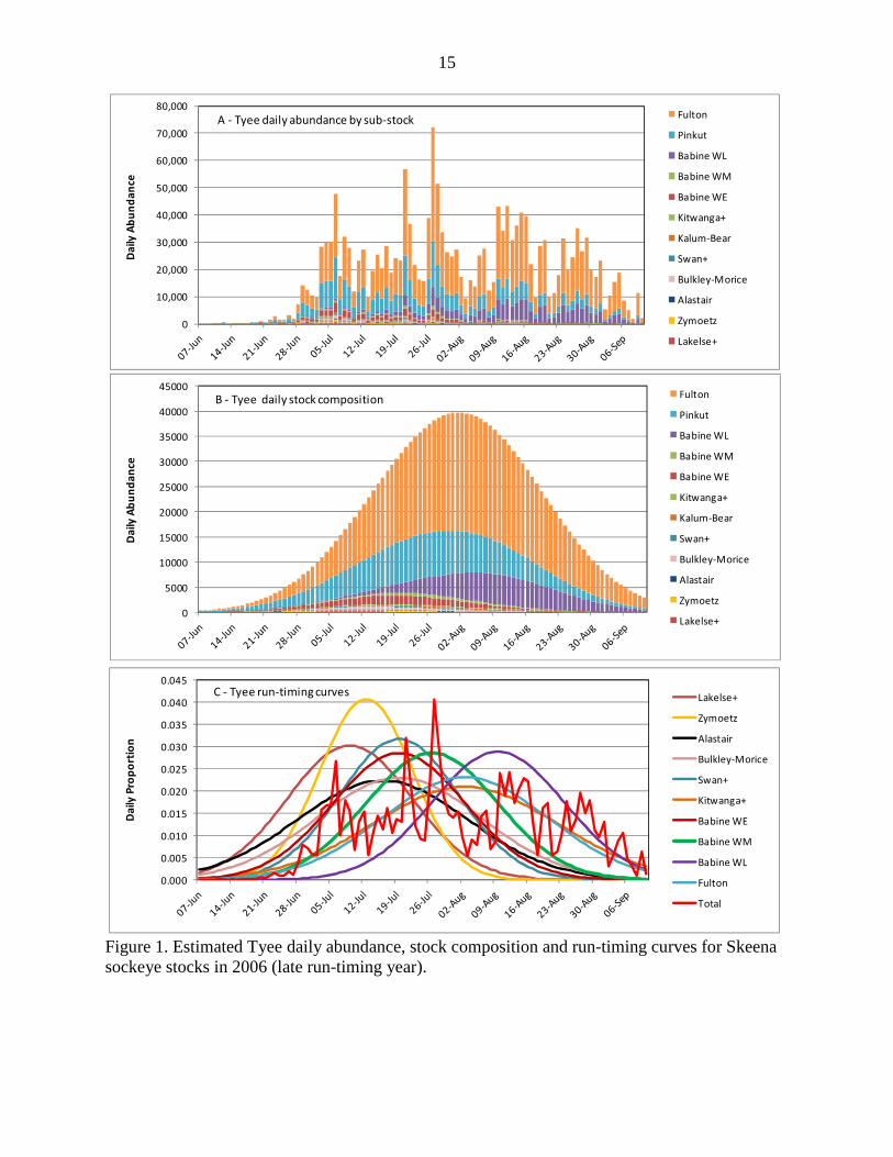
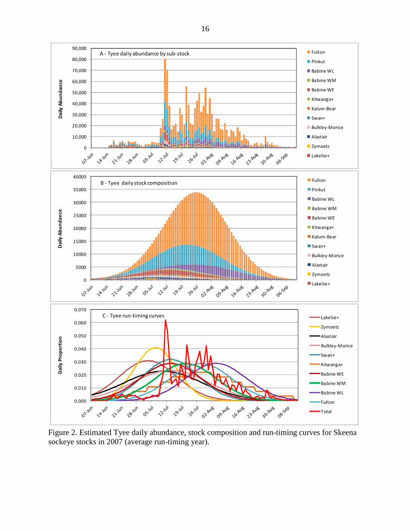
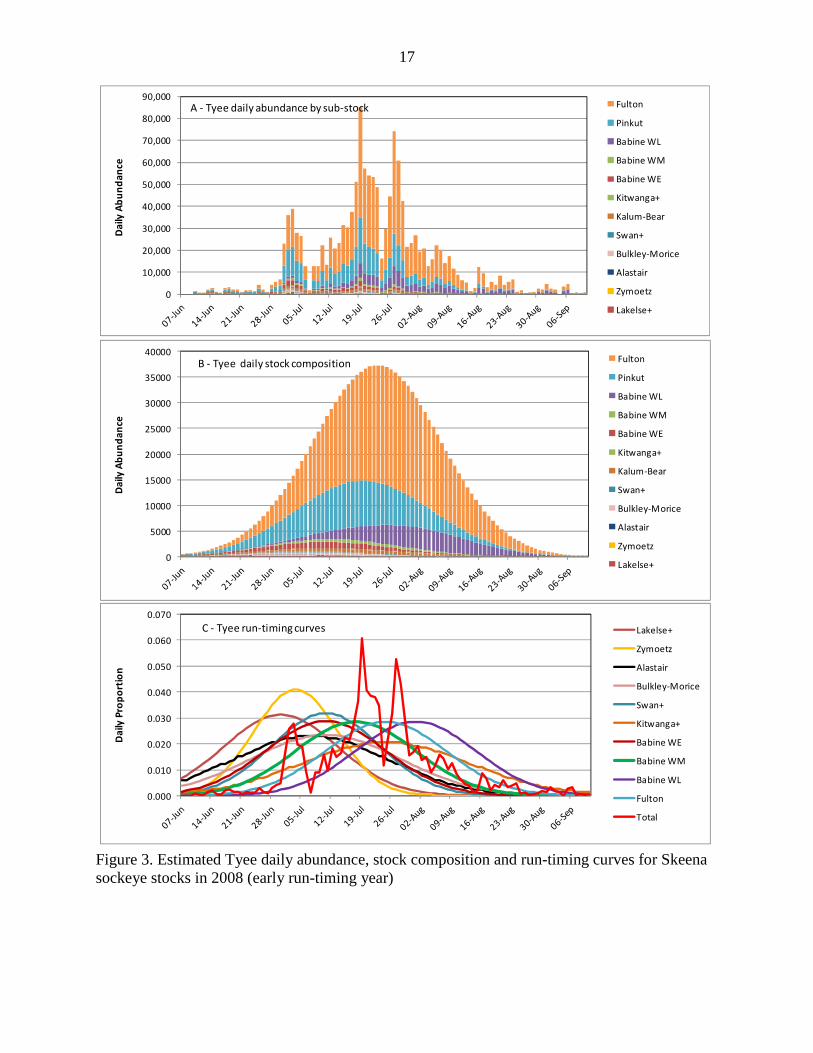
The internally documented source code for the current version of the SSIR model will be provided as an Appendix to the report for this project. 4.0 PRELIMINARY RESULTS Figures 1-3 provide a sample of the run-timing and abundance of sockeye passing the Tyee test fishery in the lower Skeena River for 2006-08. These figures also show the normally distributed run-timing curves for each of the major sub-stock groups and the resulting breakdown of the total Tyee abundance for each of the major sub-stocks. These years were selected because 2006 is an example of one of the latest run-timing years, 2007 run-timing is close to the multi-year mean and 2008 is one of the earliest run-timing years. As indicated above, 2006 was the only year where we increased the duration of two sub-stocks (Pinkut and Fulton) to reflect the protracted nature of the sockeye return in that year and ensure that the stock composition estimates for Tyee were consistent with the best available escapement estimates. These figures clearly show the substantial overlap in the run-timing and long durations estimated for most Skeena sockeye stocks. These long durations are likely the result of having to use multiple years of DNA samples to obtain an adequate sample size for the relatively small non-Babine sockeye stocks. Steve Cox-Rogers 23 February 2012 memorandum included the following conclusion:

“The estimated peak dates of run entry for most Skeena sockeye sub-stocks, based on updated 2000-2010 DNA analysis, are not substantially different from past tagging assessments and the peak dates currently being used to assess stock impacts. The DNA data does suggest slightly wider “spreads” about the peaks for most stocks than currently assumed, and some apparent skewness/bi-modal variability to the timings may not be appropriately captured with the current practice of fitting normal curve approximations to the data. However, it is not clear how much of the shape variation is real or simply an artefact of sample size issues given the small number of DNA samples actually analyzed for some stocks in certain weeks (e.g. the tails of the test fishery). This, coupled with the fact that many non-Babine stocks are present in small proportions at Tyee in the first place, means the derived timings for the larger stocks are probably ok, but will always be uncertain for the smaller ones.”

While it is likely that the run duration for a single year would be shorter than the duration derived from samples collected over multiple years, the harvest rate estimates derived from these longer run durations will be less sensitive to uncertainties in the run and harvest timing for a given year. In the absence of more reliable year specific data on run-timing and duration, a conservative approach for estimating harvest rates for in-river fisheries is to use these longer durations. Two model inputs that are critical for deriving reliable estimates of in-river harvest rates are catch estimates for all major fisheries and relative escapement estimates for each sub-stock. The preliminary estimates of the stock-specific harvest rates show the results of deficiencies in the available catch and escapement estimates (Table 6). Harvest rates estimated for lower Skeena

7

stocks in 1992 and 2001 are underestimated due to missing catch estimates for all Skeena fisheries below Terrace. Underestimation of escapements to the Bulkley-Morice watershed prior to 1989, have resulted in substantial overestimates of the harvest rates for the Moricetown fishery for 1982-1988. In years when catch estimates are available for all major fisheries and escapement estimates reflect the relative abundance of each stock, the SSIR model produces harvest rates the difference in the magnitude and location of fisheries and run-timing and geographic distribution of the sockeye sub-stocks. For example: in 2000 when ESSR fisheries were permitted to target surplus escapements for enhanced Babine stocks, in-river harvest rates were 45% for Pinkut and Fulton, 20-32% for the three run-timing groups of wild Babine sockeye, 23-27% for upper Skeena sockeye stocks and 1-4% for the early run lower Skeena sockeye stocks. In years without ESSR fisheries (e.g. 2002 and 2005), in-river harvest rates are similar (15-20%) for all Babine sockeye sub-stocks, 10-16% for upper Skeena stocks and 2-6% for lower Skeena stocks. The two lower Skeena stocks with notably shorter durations and least overlap with the Babine enhanced stocks are Lakelse and Zymoetz. The in-river harvest rates for these stocks are typically in the 2-4% range. 5.0 NEXT STEPS The tasks remaining to complete the estimation of in-river harvest rates for 1982-2009 include:

1. Circulate this report for review and discussion with Skeena River First Nations during the week of 29 October 2012;

2. Obtain additional information on in-river fisheries and fill in any missing catch estimates;

3. Discuss any necessary adjustments to the relative escapement estimates for Skeena sockeye sub-stock;

4. Discuss the model assumptions regarding run-timing and obtain additional information that could be used to improve the run-timing estimates;

5. Finalize the estimates of in-river harvest rates for each Skeena sub-stock and combine these with the marine harvest rates to compute total exploitation rates for each sub-stock from 1982-2009.

8

6.0 LITERATURE CITED Alexander, R., K.K. English, D. Peacock, and G. Oliver. 2010. Assessment of the Canadian and

Alaskan Sockeye Stocks harvested in the northern boundary fisheries using run reconstruction techniques, 2004-08. Draft report for Pacific Salmon Comm. Northern Boundary Technical Committee.

Cave J. and W.J. Gazey. 1994. A simulation model for fisheries on Fraser River sockeye

salmon. J. Fish. and Aquat. Sci. 51:1535-1549. English, K.K., T. Mochizuki and D, Robichaud. 2011. Review of North and Central Coast

Salmon Indicator Streams and Estimating Escapement, Catch and Run Size for each Salmon Conservation Unit. Report for Pacific Salmon Foundation and Fisheries and Oceans, Canada. 68 p.

English, K.K., R. E. Bailey, and D. Robichaud. 2007. Assessment of Chinook returns to the

Fraser River watershed using run reconstruction techniques, 1982-04. Canadian Science Advisory Secretariat, Research Document 2007/020. 76 p.

English, K.K., R. Alexander, D. Peacock, and G. Oliver. 2005. Assessment of the Canadian and Alaskan Sockeye Stocks harvested in the northern boundary fisheries using run reconstruction techniques, 2002-03. Prepared for Pacific Salmon Comm. Northern Boundary Technical Committee. 59 p.

English, K.K., W. J. Gazey, D. Peacock, and G. Oliver. 2004. Assessment of the Canadian and Alaskan Sockeye Stocks harvested in the northern boundary fisheries using run reconstruction techniques, 1982-2001. Pacific Salmon Comm. Tech. Rep. No. 13:93 p.

Gazey, W.J. 2009. Interception of Skeena River Sockeye salmon stocks in northern boundary

marine fisheries. Report for Skeena Wild Conservation Trust, Terrace, BC. 43 p. Gazey, W.J., and K.K. English. 2000. Assessment of sockeye and pink salmon stocks in the

northern boundary area using run reconstruction techniques, 1982-95. Can. Tech. Report Fish. Aquat. Sci. No. 2320. 132 p.

Noble, C. 2011. Assessing the performance of an in-river backward run reconstruction of Fraser

River sockeye under biological uncertainty. MRM Thesis. Simon Fraser University. 53 p.

Starr, P. and R. Hilborn. 1988. Reconstruction of harvest rates and stock contribution in

gauntlet salmon fisheries: application to British Columbia and Washington sockeye (Oncorhynchus nerka). Can J. Fish. Aquat. Sci 45: 2216-2229.

9 Table 1. Fisheries, stocks and estimates residence time in days for the Skeena sockeye in-river run reconstruction analyses.

Fisheries

Stocks (Geographic CUs) Short Name Ord

er

Ag

gre

ga

te

Da

ta Q

ua

lity1

CU

s in

Gro

up

Co

ast

al t

o K

asi

ks

Ka

siks

-Te

rra

ce

Te

rra

ce-F

idd

ler

Fid

dle

r-H

aze

lton

Ha

zelto

n-L

Ba

bin

e

Ba

bin

e b

elo

w F

en

ce

Ba

bin

e F

en

ce

Ba

bin

e L

ake

Pin

kut

Te

rmin

al

Fu

lton

Te

rmin

al

Bu

lkle

y-M

oric

e

Su

stu

t

Kluatantan/Kluayaz Kluatan+ 1 1 W 2 3 4 3 4 7Motase Motase 2 1 W 1 3 4 3 4 7Sustut/Johanson/Spawning Sustut+ 3 1 G 3 3 4 3 4 7 1

Bear/Azuklotz/Asitka Bear+ 4 1 G 3 3 4 3 4 7Slamgeesh/Damshilgwit Slamgeesh 5 1 G 2 3 4 3 4 7Sicintine Sicintine 6 1 W 1 3 4 3 4 7Babine W Early Babine-WE 7 2 G 1 3 4 3 4 7 4 1 3Babine W Middle Babine-WM 8 2 G 1 3 4 3 4 7 4 1 3Babine W Late Babine-WL 9 2 G 1 3 4 3 4 7 4 1 3Babine Pinkut Babine-P 10 2 G 1 3 4 3 4 7 4 1 3 1Babine Fulton Babine-F 11 2 G 1 3 4 3 4 7 4 1 3 1Swan/Stephans/Club Swan+ 12 1 G 3 3 4 3 4Bulkley/Maxan Bulkley+ 13 1 W 2 3 4 3 4 1Morice/Atna Morice+ 14 1 G 2 3 4 3 4 1Kitwanga Kitwanga 15 1 G 1 3 4 3 2Zymoetz Zymoetz 16 1 W 3 3 4 1Kalum Kalum 17 1 W 1 3 4Lakelse Lakelse 18 1 G 1 3 4Alastair Alastair 19 1 G 1 3Johnston Johnston 20 1 W 1 1

1 G= Good, W=Weak

10

Table 2. Escapement estimates for each sub-stock of Skeena sockeye salmon 1980-2010.

Klu

ata

n+

Mo

tase

Su

stu

t+

Be

ar+

Sla

mg

ee

sh

Sic

intin

e

Ba

bin

e-W

E

Ba

bin

e-W

M

Ba

bin

e-W

L

Ba

bin

e-P

Ba

bin

e-F

Sw

an

+

Bu

lkle

y+

Mo

rice

+

Kitw

an

ga

Zym

oe

tz

Ka

lum

Lake

lse

Ala

sta

ir

Joh

nst

on

Ske

en

a A

gg

.

1980 1,000 500 4,000 1,980 1,000 1,000 31,679 11,166 197,03185,017 178,731 3,166 1,000 850 200 280 620 29,620 30,000 504 579,3441981 1,000 500 4,000 997 1,000 1,000 46,466 7,178 113,332 453,885 781,574 8,443 1,000 2,125 1,040 3,000 482 16,064 1,800 504 1,445,3891982 1,000 500 4,000 947 1,000 1,000 93,630 4,827 159,595 231,341 605,442 8,443 1,000 6,375 1,880 2,000 758 30,296 9,500 504 1,164,0371983 1,000 500 4,000 922 1,000 1,000 26,965 8,904 103,027 191,903 535,594 9,498 1,000 8,500 2,720 10,000 606 19,365 13,000 705 940,2101984 1,000 500 4,000 897 1,000 1,000 26,503 8,065 204,447 357,780 435,090 10,553 1,000 6,375 3,560 1,000 785 9,573 8,000 705 1,081,8331985 1,000 500 4,000 2,709 1,000 1,000 75,649 17,229 623,637590,887 823,141 9,287 1,000 4,250 4,400 1,200 1,570 36,530 8,000 907 2,207,8961986 1,000 500 4,000 2,992 1,000 1,000 26,865 3,874 167,437 213,745 266,086 10,553 1,000 6,375 3,720 6,000 1,570 9,022 21,000 353 748,0921987 1,000 1,500 4,000 10,917 1,000 1,000 38,206 15,786 237,400 665,019 331,145 21,107 1,000 8,500 3,040 6,000 3,139 5,336 10,000 604 1,365,6991988 1,000 100 4,000 7,221 1,000 1,000 42,435 23,459 241,974376,474 699,538 25,328 1,000 2,125 2,360 4,000 1,884 10,50813,000 705 1,459,1091989 1,000 400 4,000 1,667 1,000 1,000 18,412 7,701 132,563 233,680 717,960 8,443 1,000 11,900 1,680 3,500 2,825 7,724 14,932 302 1,171,6901990 1,000 60 4,000 2,279 1,000 1,000 21,328 7,395 198,864 202,042 527,016 10,553 1,000 12,750 1,000 3,000 4,133 2,707 10,000 458 1,011,5861991 1,000 300 4,000 7,551 1,000 1,000 58,719 24,980 432,582437,123 202,114 14,775 1,000 85,001 1,000 1,200 4,133 13,534 22,000 613 1,313,6241992 1,000 500 4,000 5,097 1,000 1,000 55,071 8,863 613,114 457,238 734,513 21,107 1,000 57,376 1,000 10,000 11,022 10,453 16,000 1,992 2,011,3461993 1,000 400 4,000 5,599 1,000 1,000 16,646 21,962 595,377455,190 470,660 16,885 1,000 46,751 1,000 15,000 9,645 13,754 15,000 3,371 1,695,2401994 1,000 250 4,000 8,057 1,000 1,000 25,124 7,560 132,299 202,916 636,540 12,453 1,000 60,563 1,000 10,295 15,156 3,136 13,000 4,750 1,141,1001995 1,000 250 4,000 10,516 1,000 1,000 79,679 6,555 69,506 565,722 916,955 8,020 1,000 74,376 500 10,295 13,434 27,618 17,000 6,129 1,814,5541996 1,000 100 4,000 6,308 1,000 1,000 60,909 7,975 143,305 518,865 917,303 7,598 1,000 87,126 250 10,295 5,236 23,822 25,000 5,108 1,827,1981997 1,000 220 4,000 3,816 1,000 1,000 92,245 34,660 129,975184,561 488,761 5,910 1,000 51,001 250 10,295 10,058 3,466 24,000 4,086 1,051,3031998 1,000 500 4,000 1,578 1,000 1,000 43,130 16,545 97,880 97,149 244,797 5,910 1,000 12,750 250 10,295 10,747 5,409 11,000 6,129 572,0701999 1,000 500 4,000 9,195 1,000 1,000 63,692 22,946 155,040132,582 208,657 4,221 1,000 31,875 250 10,295 12,318 7,235 2,000 8,172 676,9772000 1,000 400 4,000 5,297 949 1,000 84,558 19,982 185,020 197,387 888,911 5,823 1,000 6,375 231 10,295 13,888 7,235 6,200 1,500 1,441,0502001 1,000 200 4,000 4,348 855 1,000 232,802 47,818 617,401 114,385 462,095 7,425 1,000 8,500 221 10,295 8,292 9,061 10,800 4,500 1,545,9972002 1,000 100 4,000 897 398 1,000 37,049 31,046 165,162 83,236 253,749 2,533 1,000 14,875 978 7,072 11,072 7,468 4,000 2,000 628,6352003 1,000 2,000 4,992 11,253 430 1,000 55,028 83,151 99,284218,006 682,889 5,070 1,000 21,250 3,377 9,106 28,383 7,46827,000 5,050 1,266,7382004 1,000 600 1,604 2,998 293 1,000 45,849 59,994 288,950 92,033 401,164 5,538 1,000 16,469 1,317 6,332 13,968 5,875 20,074 2,395 968,453

2005 1,000 290 1,175 2,499 216 1,000 27,153 33,882 176,235 123,965 314,847 2,550 1,000 17,002 937 6,888 8,939 6,305 13,147 2,395 741,4252006 1,000 120 808 2,849 331 1,000 40,874 12,515 137,660 258,670 684,130 4,529 1,000 17,536 5,139 6,116 9,521 3,632 4,8002,395 1,194,6252007 1,000 300 2,469 3,199 366 1,000 52,862 12,595 100,762 226,528 607,886 2,090 1,000 28,475 245 3,800 12,455 6,624 22,000 2,395 1,088,0522008 1,000 100 212 8,577 150 1,000 28,667 12,744 93,158 197,787 507,968 4,475 1,000 19,125 1,200 280 15,349 5,513 1,119 2,395 901,8192009 1,000 410 540 6,787 161 1,000 20,503 18,341 93,791 140,515 340,254 3,466 1,000 24,342 3,047 3,400 19,521 7,574 21,500 2,395 709,5482010 1,000 592 426 12,210 740 1,000 20,455 6,065 74,126 133,695 361,259 266 1,000 7,831 20,804 2,980 30,496 14,720 33,7002,395 725,760

After FillAverage 1,000 442 3,362 4,908 1,000 1,000 51,263 19,541 218,708 272,236 523,444 8,581 1,000 24,475 2,213 6,275 9,097 11,827 14,470 2,465 1,177,110

Portion 0.001 0.000 0.003 0.004 0.001 0.001 0.044 0.017 0.186 0.231 0.445 0.007 0.001 0.021 0.002 0.005 0.008 0.010 0.0120.002Before Fill

Average 0 441 1,528 5,080 444 0 51,263 19,541 218,708 272,236523,444 8,709 0 23,796 3,078 4,939 8,990 12,490 14,283 2,3951,171,365Portion 0.001 0.000 0.003 0.004 0.001 0.001 0.044 0.017 0.187 0.232 0.447 0.007 0.001 0.020 0.003 0.004 0.008 0.011 0.0120.002

11 Table 3. Run-timing parameters used for each Skeena sockeye sub-stock group.

Source: Cox-Rogers (2012)

# Stocks (Geographic CUs) CU

s in

Gro

up

Off

set

(da

ys)

Du

ratio

n (

da

ys)

De

fau

lt S

D (

da

ys)

20

06

SD

(d

ays

)

Group Name Pea

k W

eek

Off

set

(da

ys)

SD

(w

ee

ks)

1 Kluatantan/Kluayaz 2 -10.5 105 17.5 17.5 Bulkley-Morice 72 -10.5 2.52 Motase 1 3.5 92 15.4 15.4 Motase 74 3.5 2.23 Sustut/Johanson/Spawning 3 -3.5 84 14.0 14.0 Sustut 73 -3.5 2.04 Bear/Azuklotz/Asitka 3 -3.5 84 14.0 14.0 Sustut 73 -3.5 2.05 Slamgeesh/Damshilgwit 2 -3.5 84 14.0 14.0 Sustut 73 -3.5 2.06 Sicintine 1 -3.5 84 14.0 14.0 Sustut 73 -3.5 2.07 Babine W Early 1 -10.5 84 14.0 14.0 Babine WE 72 -10.5 2.08 Babine W Middle 1 -3.5 84 14.0 14.0 Babine WM 73 -3.5 2.09 Babine W Late 1 10.5 84 14.0 14.0 Babine WL 75 10.5 2.010 Babine Pinkut 1 -3.5 84 14.0 17.5 Pinkut 73 -3.5 2.011 Babine Fulton 1 3.5 84 14.0 17.5 Fulton 73 3.5 2.012 Swan/Stephans/Club 3 -10.5 76 12.6 12.6 Swan+ 72 -10.5 1.813 Bulkley/Maxan 2 -10.5 105 17.5 17.5 Bulkley-Morice 72 -10.5 2.514 Morice/Atna 2 -10.5 105 17.5 17.5 Bulkley-Morice 72 -10.52.515 Kitwanga 1 3.5 118 19.6 19.6 Kitwanga+ 74 3.5 2.816 Zymoetz 3 -17.5 59 9.8 9.8 Zymoetz 71 -17.5 1.417 Kalum 1 -3.5 105 17.5 17.5 Kalum-Bear 73 -3.5 2.518 Lakelse 1 -21.0 80 13.3 13.3 Lakelse+ 64 -21 1.919 Alastair 1 -14.0 109 18.2 18.2 Alastair 71 -14 2.620 Johnston 1 -21.0 80 13.3 13.3 Lakelse+ 64 -21 1.9

12 Table 4. Annual estimates of the harvest of Skeena River sockeye by First Nations in FSC fisheries, 1982-2009. Fishery Group 1982 1983 1984 1985 1986 1987 1988 1989 1990 1991 1992 1993 1994 1995

Coastal TTC 12,770 7,232 7,630 10,655 8,284 9,431 7,334 8,553 10,197 5,420 16,926 8,423 11,821Marine to Kasiks TTC 23,816 13,489 14,230 19,872 15,450 17,590 13,678 15,951 19,017 10,108 27,809 26,409 14,905

Coastal to Kasiks TTC 36,586 20,721 21,860 30,526 23,734 27,021 21,012 24,504 29,214 15,528 44,735 34,832 26,726Kasiks to Terrace TTC 4,582 2,595 2,738 3,823 2,972 3,384 2,631 3,069 3,658 1,945 14,274 3,665 5,177Terrace to Fiddler TTC 11,653 6,600 6,963 9,723 7,560 8,606 6,693 7,805 9,305 4,946 9,019 14,418 9,757Fiddler to Hazelton GWWA 102,600 79,420 128,250 114,000 85,500 76,000 71,250 85,500 83,600 83,600 66,500 27,221 35,307 42,668Hazelton to L. BabineGWWA 5,400 4,180 6,750 6,000 4,500 4,000 3,750 4,500 4,400 4,400 3,500 1,858 2,246Babine below Fence GWWA 13,448 6,439Babine Fence LBNBabine Lake LB/YECH 42,000 20,000 12,100 16,000 4,050 25,000 22,000 27,008 15,650 33,093 68,250 32,300 18,491Pinkut Terminal LBNFulton Terminal LBNBulkley-Morice GWWA 4,500 6,450 4,000 22,450 20,296 4,250 1,450 13,000 15,138 11,408 12,629 23,912Sustut TAKLA 1,302

Total 207,320 139,966 178,660 184,072 150,766 139,307 134,586 148,828 157,185 139,069 118,231 188,355 136,311 135,416

Fishery Group 1996 1997 1998 1999 2000 2001 2002 2003 2004 2005 2006 2007 2008 2009

Coastal TTC 7,444 4,090 21,124 3,073 37,157 29,000 3,123 4,356 10,376 9,607 21,685 27,134 9,100Marine to Kasiks TTC 31,951 37,839 24,105 14,644 27,600 20,000 4,840 2,507 17,022 5,428

Coastal to Kasiks TTC 39,395 41,929 45,229 17,717 64,757 49,000 3,123 9,196 12,883 9,607 38,707 32,562 9,100Kasiks to Terrace TTC 5,927 4,656 1,951 2,294 1,544 4,905 6,075 7,056 4,360 5,803 4,168 5,966 10,763Terrace to Fiddler TTC 15,744 12,909 15,209 10,131 13,24513,479 13,680 11,337 12,550 9,098 9,749 9,338 8,535 9,465Fiddler to Hazelton GWWA 21,058 32,880 50,369 51,854 58,444 49,531 56,258 60,876 66,295 64,144 68,859 26,306 63,494 35,946Hazelton to L. BabineGWWA 1,109 1,731 2,651 2,730 3,076 2,487 2,879 3,204 3,489 3,376 3,624 1,385 3,342 1,892Babine below Fence GWWA 2,802 1,637 195 3,366 2,658 5,000 1,091 533 333 1,273 16,643 107Babine Fence LBNBabine Lake LB/YECH 39,422 13,699 9,744 23,220 23,300 24,080 24,785 32,000 31,441 33,117 38,600 36,070 48,901 43,957Pinkut Terminal LBNFulton Terminal LBNBulkley-Morice GWWA 14,453 15,512 3,674 675 1,905 1,289 331 456 278 197 2,085 219 2,391 1,644Sustut TAKLA 559 513 768 868 1,050 470 811 1,954 567 862 632 419 526 992

Total 140,469 125,466 129,790 112,855 169,979 96,336 153,740 119,558 131,205 129,310 138,959 133,254 165,717 113,866

1) Coastal = LaxKwalaams+Metlakatla (No Kitkatla+Hartley Bay) catch data2) Marine to Kasiks = Prince Rupert catch data3) Kasiks to Terrace = Kitsumkalum catch data4) Terrace to Fiddler = Kitselas catch data5) Fiddler to Hazelton = 0.95 * Skeena (e.g. Hazelton) catch data based on comments provided by J. Steward regarding location of catch + Gitanyow6) Hazelton to Lower Babine = 0.05 * Skeena (e.g. Hazelton) catch data based on comments provided by J.Steward regrading location of catch7) Kitsegass (L. Babine) = Babine catch data8) All Babine Lake = sum of Nat'oo'ten catch data 9) Sustut = Takla catch data10) 1982-1992 GWWA Kitsegass catch data are included in the Hazelton to Lower Babine catch estimates11) 1982-2000 Moricetown data are the actual reported catch figures12) Note: Some missing 1992-1982 catch by fishery calculated as area-specific IFF total catch*Prop. IFF catch for 1993-2000These numbers are of unknown accuracy: all have been interpolated from Kerra Hoyseth's (2000) DFO review.USE WITH CAUTION

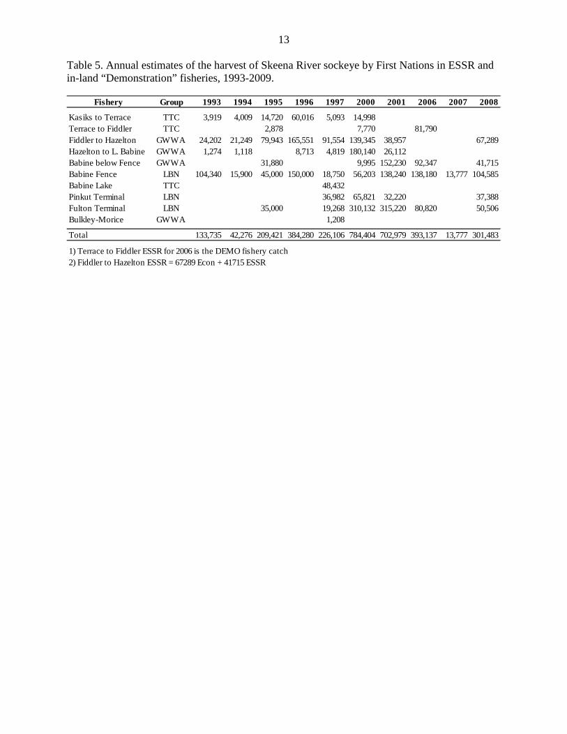
13 Table 5. Annual estimates of the harvest of Skeena River sockeye by First Nations in ESSR and in-land “Demonstration” fisheries, 1993-2009.

Fishery Group 1993 1994 1995 1996 1997 2000 2001 2006 2007 2008

Kasiks to Terrace TTC 3,919 4,009 14,720 60,016 5,093 14,998Terrace to Fiddler TTC 2,878 7,770 81,790Fiddler to Hazelton GWWA 24,202 21,249 79,943 165,551 91,554 139,345 38,957 67,289Hazelton to L. Babine GWWA 1,274 1,118 8,713 4,819 180,140 26,112Babine below Fence GWWA 31,880 9,995 152,230 92,347 41,715Babine Fence LBN 104,340 15,900 45,000 150,000 18,750 56,203 138,240 138,180 13,777 104,585Babine Lake TTC 48,432Pinkut Terminal LBN 36,982 65,821 32,220 37,388Fulton Terminal LBN 35,000 19,268 310,132 315,220 80,820 50,506Bulkley-Morice GWWA 1,208

Total 133,735 42,276 209,421 384,280 226,106 784,404 702,979 393,137 13,777 301,483

1) Terrace to Fiddler ESSR for 2006 is the DEMO fishery catch 2) Fiddler to Hazelton ESSR = 67289 Econ + 41715 ESSR

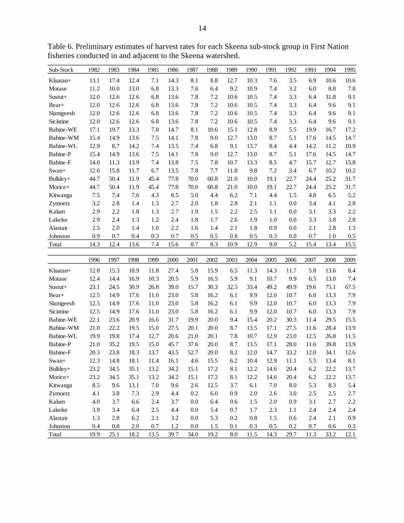
14 Table 6. Preliminary estimates of harvest rates for each Skeena sub-stock group in First Nation fisheries conducted in and adjacent to the Skeena watershed.

Sub-Stock 1982 1983 1984 1985 1986 1987 1988 1989 1990 1991 1992 1993 1994 1995

Kluatan+ 13.1 17.4 12.4 7.1 14.3 8.1 8.8 12.7 10.3 7.6 3.5 6.9 10.6 10.6Motase 11.2 10.0 13.0 6.8 13.3 7.6 6.4 9.2 10.9 7.4 3.2 6.0 8.8 7.8Sustut+ 12.0 12.6 12.6 6.8 13.6 7.8 7.2 10.6 10.5 7.4 3.3 6.4 31.8 9.1Bear+ 12.0 12.6 12.6 6.8 13.6 7.8 7.2 10.6 10.5 7.4 3.3 6.4 9.6 9.1Slamgeesh 12.0 12.6 12.6 6.8 13.6 7.8 7.2 10.6 10.5 7.4 3.3 6.49.6 9.1Sicintine 12.0 12.6 12.6 6.8 13.6 7.8 7.2 10.6 10.5 7.4 3.3 6.49.6 9.1Babine-WE 17.1 19.7 13.3 7.8 14.7 8.1 10.6 15.1 12.8 8.9 5.5 19.9 16.7 17.2Babine-WM 15.4 14.9 13.6 7.5 14.1 7.8 9.0 12.7 13.0 8.7 5.1 17.6 14.5 14.7Babine-WL 12.9 8.7 14.2 7.4 13.5 7.4 6.8 9.1 13.7 8.4 4.4 14.2 11.2 10.9Babine-P 15.4 14.9 13.6 7.5 14.1 7.8 9.0 12.7 13.0 8.7 5.1 17.614.5 14.7Babine-F 14.0 11.3 13.9 7.4 13.8 7.5 7.8 10.7 13.3 8.5 4.7 15.712.7 15.8Swan+ 12.6 15.8 11.7 6.7 13.5 7.8 7.7 11.8 9.8 7.2 3.4 6.7 10.2 10.2Bulkley+ 44.7 50.4 11.9 45.4 77.8 70.0 60.8 21.0 10.0 19.1 22.7 24.4 25.2 31.7Morice+ 44.7 50.4 11.9 45.4 77.8 70.0 60.8 21.0 10.0 19.1 22.724.4 25.2 31.7Kitwanga 7.5 7.4 7.6 4.3 8.5 5.0 4.4 6.2 7.1 4.4 1.5 4.8 6.5 5.2Zymoetz 3.2 2.8 1.4 1.3 2.7 2.0 1.8 2.8 2.1 1.1 0.0 3.4 4.1 2.8Kalum 2.9 2.2 1.8 1.3 2.7 1.9 1.5 2.2 2.5 1.1 0.0 3.1 3.3 2.2Lakelse 2.9 2.4 1.3 1.2 2.4 1.8 1.7 2.6 1.9 1.0 0.0 3.3 3.8 2.8Alastair 2.5 2.0 1.4 1.0 2.2 1.6 1.4 2.1 1.8 0.9 0.0 2.1 2.8 1.3Johnston 0.9 0.7 0.4 0.3 0.7 0.5 0.5 0.8 0.5 0.3 0.0 0.7 1.0 0.5Total 14.3 12.4 13.6 7.4 15.6 8.7 8.3 10.9 12.9 9.0 5.2 15.4 13.4 15.5

1996 1997 1998 1999 2000 2001 2002 2003 2004 2005 2006 2007 2008 2009

Kluatan+ 12.8 15.3 18.9 11.8 27.4 5.8 15.9 6.5 11.3 14.3 11.7 5.8 13.6 8.4Motase 12.4 14.4 16.9 10.3 20.5 5.9 16.5 5.9 9.1 10.7 9.9 6.5 13.0 7.4Sustut+ 23.1 24.5 30.9 26.8 39.0 15.7 30.3 32.5 33.4 49.2 49.919.6 75.1 67.5Bear+ 12.5 14.9 17.6 11.0 23.0 5.8 16.2 6.1 9.9 12.0 10.7 6.0 13.3 7.9Slamgeesh 12.5 14.9 17.6 11.0 23.0 5.8 16.2 6.1 9.9 12.0 10.7 6.0 13.3 7.9Sicintine 12.5 14.9 17.6 11.0 23.0 5.8 16.2 6.1 9.9 12.0 10.7 6.0 13.3 7.9Babine-WE 22.1 23.6 20.9 16.6 31.7 19.9 20.0 9.4 15.4 20.2 30.3 11.4 29.5 15.5Babine-WM 21.0 22.2 19.5 15.0 27.5 20.1 20.0 8.7 13.5 17.1 27.5 11.6 28.4 13.9Babine-WL 19.9 19.8 17.4 12.7 20.6 21.0 20.1 7.8 10.7 12.9 23.0 12.5 26.8 11.5Babine-P 21.0 35.2 19.5 15.0 45.7 37.6 20.0 8.7 13.5 17.1 28.011.6 39.8 13.9Babine-F 20.3 23.8 18.3 13.7 43.5 52.7 20.0 8.2 12.0 14.7 33.212.0 34.1 12.6Swan+ 12.3 14.8 18.1 11.4 16.1 4.6 15.5 6.2 10.4 12.9 11.1 5.5 13.4 8.1Bulkley+ 23.2 34.5 35.1 13.2 34.2 15.1 17.2 8.1 12.2 14.6 20.46.2 22.2 13.7Morice+ 23.2 34.5 35.1 13.2 34.2 15.1 17.2 8.1 12.2 14.6 20.4 6.2 22.2 13.7Kitwanga 8.5 9.6 13.1 7.0 9.6 2.6 12.5 3.7 6.1 7.0 8.0 5.3 8.3 5.4Zymoetz 4.1 3.8 7.3 2.9 4.4 0.2 6.0 0.9 2.0 2.6 3.0 2.5 2.5 2.7Kalum 4.0 3.7 6.6 2.4 3.7 0.0 6.4 0.6 1.5 2.0 0.9 3.1 2.7 2.2Lakelse 3.9 3.4 6.4 2.5 4.4 0.0 5.4 0.7 1.7 2.3 1.1 2.4 2.4 2.4Alastair 1.3 2.8 6.2 2.1 3.2 0.0 5.3 0.2 0.8 1.5 0.6 2.4 2.1 0.9Johnston 0.4 0.8 2.0 0.7 1.2 0.0 1.5 0.1 0.3 0.5 0.2 0.7 0.6 0.3Total 19.9 25.1 18.2 13.5 39.7 34.0 19.2 8.0 11.5 14.3 29.7 11.3 33.2 12.1

15

0

5000

10000

15000

20000

25000

30000

35000

40000

45000

Da

ily

Ab

un

da

nce

Fulton

Pinkut

Babine WL

Babine WM

Babine WE

Kitwanga+

Kalum-Bear

Swan+

Bulkley-Morice

Alastair

Zymoetz

Lakelse+

B - Tyee daily stock composition

0.000

0.005

0.010

0.015

0.020

0.025

0.030

0.035

0.040

0.045

Da

ily P

rop

ort

ion

Lakelse+

Zymoetz

Alastair

Bulkley-Morice

Swan+

Kitwanga+

Babine WE

Babine WM

Babine WL

Fulton

Total

C - Tyee run-timing curves

0

10,000

20,000

30,000

40,000

50,000

60,000

70,000

80,000

Da

ily A

bu

nd

an

ce

Fulton

Pinkut

Babine WL

Babine WM

Babine WE

Kitwanga+

Kalum-Bear

Swan+

Bulkley-Morice

Alastair

Zymoetz

Lakelse+

A - Tyee daily abundance by sub-stock

Figure 1. Estimated Tyee daily abundance, stock composition and run-timing curves for Skeena sockeye stocks in 2006 (late run-timing year).

16

0

5000

10000

15000

20000

25000

30000

35000

40000

Da

ily

Ab

un

da

nce

Fulton

Pinkut

Babine WL

Babine WM

Babine WE

Kitwanga+

Kalum-Bear

Swan+

Bulkley-Morice

Alastair

Zymoetz

Lakelse+

B - Tyee daily stock composition

0.000

0.010

0.020

0.030

0.040

0.050

0.060

0.070

Da

ily

Pro

po

rtio

n

Lakelse+

Zymoetz

Alastair

Bulkley-Morice

Swan+

Kitwanga+

Babine WE

Babine WM

Babine WL

Fulton

Total

C - Tyee run-timing curves

0

10,000

20,000

30,000

40,000

50,000

60,000

70,000

80,000

90,000

Da

ily

Ab

un

da

nce

Fulton

Pinkut

Babine WL

Babine WM

Babine WE

Kitwanga+

Kalum-Bear

Swan+

Bulkley-Morice

Alastair

Zymoetz

Lakelse+

A - Tyee daily abundance by sub-stock

Figure 2. Estimated Tyee daily abundance, stock composition and run-timing curves for Skeena sockeye stocks in 2007 (average run-timing year).

17

0

5000

10000

15000

20000

25000

30000

35000

40000

Da

ily

Ab

un

da

nce

Fulton

Pinkut

Babine WL

Babine WM

Babine WE

Kitwanga+

Kalum-Bear

Swan+

Bulkley-Morice

Alastair

Zymoetz

Lakelse+

B - Tyee daily stock composition

0.000

0.010

0.020

0.030

0.040

0.050

0.060

0.070

Da

ily P

rop

ort

ion

Lakelse+

Zymoetz

Alastair

Bulkley-Morice

Swan+

Kitwanga+

Babine WE

Babine WM

Babine WL

Fulton

Total

C - Tyee run-timing curves

0

10,000

20,000

30,000

40,000

50,000

60,000

70,000

80,000

90,000

Da

ily A

bu

nd

an

ce

Fulton

Pinkut

Babine WL

Babine WM

Babine WE

Kitwanga+

Kalum-Bear

Swan+

Bulkley-Morice

Alastair

Zymoetz

Lakelse+

A - Tyee daily abundance by sub-stock

Figure 3. Estimated Tyee daily abundance, stock composition and run-timing curves for Skeena sockeye stocks in 2008 (early run-timing year)