utdallas.edu/~metin

1

Levers to Increase Profits

utdallas.edu/~metin 2

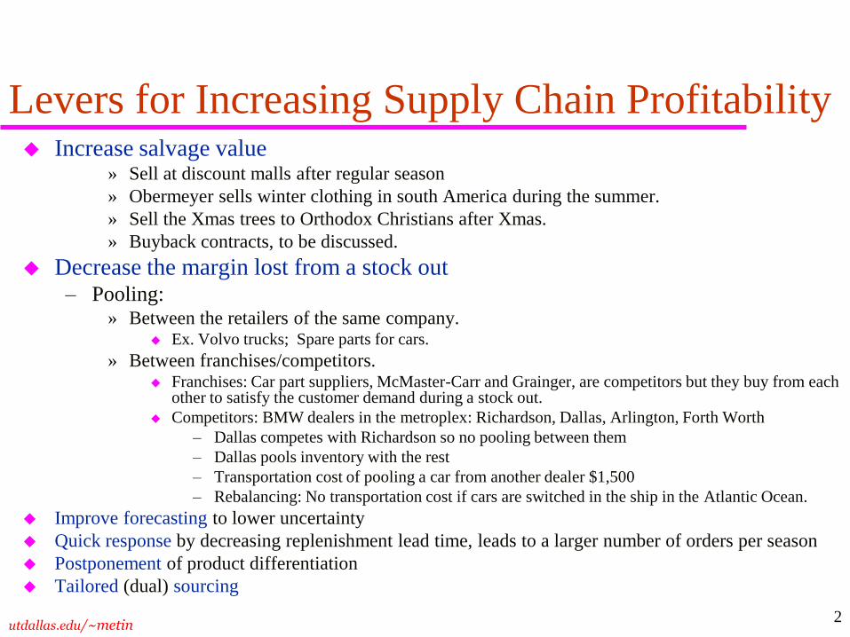
Levers for Increasing Supply Chain Profitability Increase salvage value

» Sell at discount malls after regular season

» Obermeyer sells winter clothing in south America during the summer.

» Sell the Xmas trees to Orthodox Christians after Xmas.

» Buyback contracts, to be discussed.

Decrease the margin lost from a stock out – Pooling:

» Between the retailers of the same company. Ex. Volvo trucks; Spare parts for cars.

» Between franchises/competitors. Franchises: Car part suppliers, McMaster-Carr and Grainger, are competitors but they buy from each

other to satisfy the customer demand during a stock out.

Competitors: BMW dealers in the metroplex: Richardson, Dallas, Arlington, Forth Worth

– Dallas competes with Richardson so no pooling between them

– Dallas pools inventory with the rest

– Transportation cost of pooling a car from another dealer $1,500

– Rebalancing: No transportation cost if cars are switched in the ship in the Atlantic Ocean.

Improve forecasting to lower uncertainty

Quick response by decreasing replenishment lead time, leads to a larger number of orders per season

Postponement of product differentiation

Tailored (dual) sourcing

utdallas.edu/~metin

3

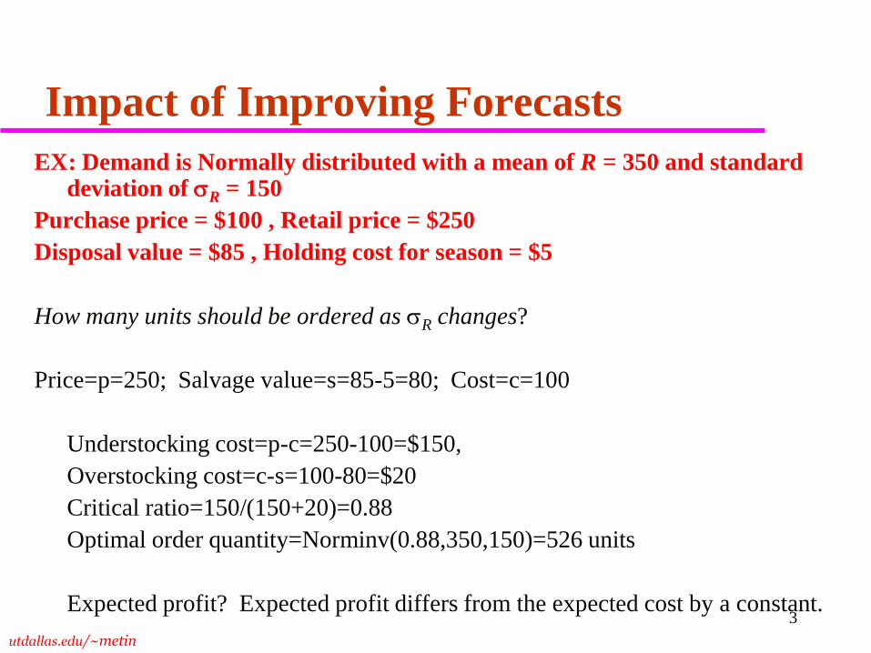
Impact of Improving Forecasts

EX: Demand is Normally distributed with a mean of R = 350 and standard deviation of R = 150

Purchase price = $100 , Retail price = $250

Disposal value = $85 , Holding cost for season = $5

How many units should be ordered as R changes?

Price=p=250; Salvage value=s=85-5=80; Cost=c=100

Understocking cost=p-c=250-100=$150,

Overstocking cost=c-s=100-80=$20

Critical ratio=150/(150+20)=0.88

Optimal order quantity=Norminv(0.88,350,150)=526 units

Expected profit? Expected profit differs from the expected cost by a constant.

utdallas.edu/~metin

4

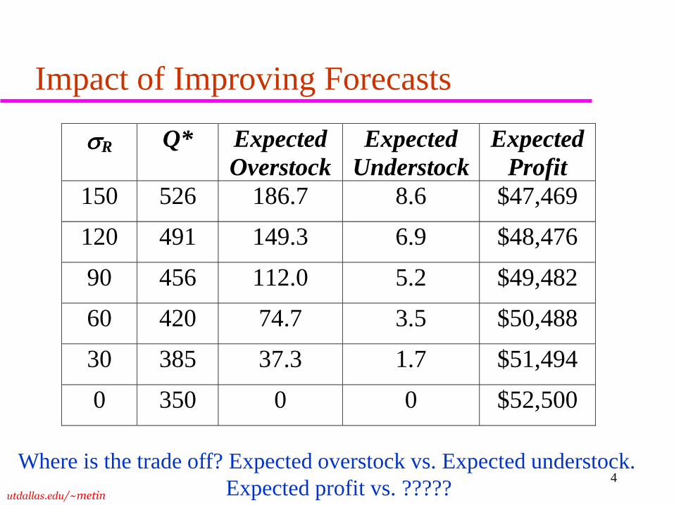
Impact of Improving Forecasts

R Q* Expected

Overstock

Expected

Understock

Expected

Profit

150 526 186.7 8.6 $47,469

120 491 149.3 6.9 $48,476

90 456 112.0 5.2 $49,482

60 420 74.7 3.5 $50,488

30 385 37.3 1.7 $51,494

0 350 0 0 $52,500

Where is the trade off? Expected overstock vs. Expected understock.

Expected profit vs. ?????

utdallas.edu/~metin

5

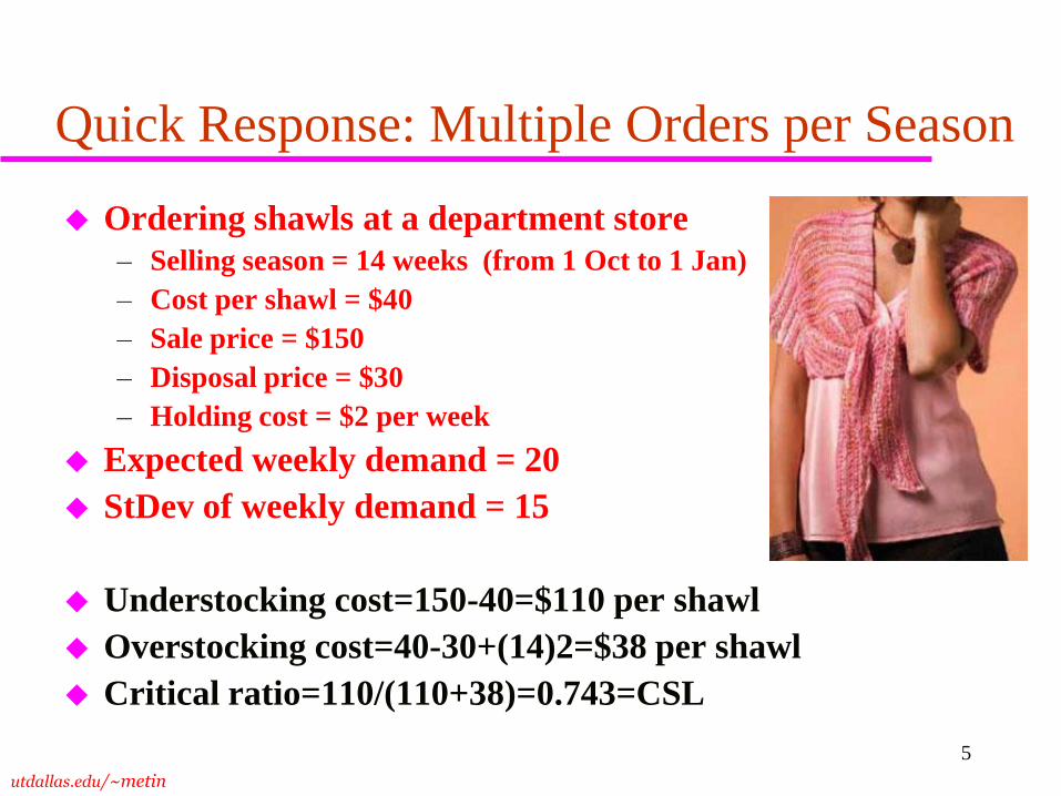
Quick Response: Multiple Orders per Season

Ordering shawls at a department store

– Selling season = 14 weeks (from 1 Oct to 1 Jan)

– Cost per shawl = $40

– Sale price = $150

– Disposal price = $30

– Holding cost = $2 per week

Expected weekly demand = 20

StDev of weekly demand = 15

Understocking cost=150-40=$110 per shawl

Overstocking cost=40-30+(14)2=$38 per shawl

Critical ratio=110/(110+38)=0.743=CSL

utdallas.edu/~metin

6

Ordering Twice as Opposed to Once

The second order can be used to correct the demand supply mismatch in the first order

– At the time of placing the second order, take out the on-hand inventory from the demand the second order is supposed to satisfy. This is a simple inventory correction idea.

Between the times the first and the second orders are placed, more information becomes available to demand forecasters. The second order is typically made against less uncertainty than the first order is.

utdallas.edu/~metin 7

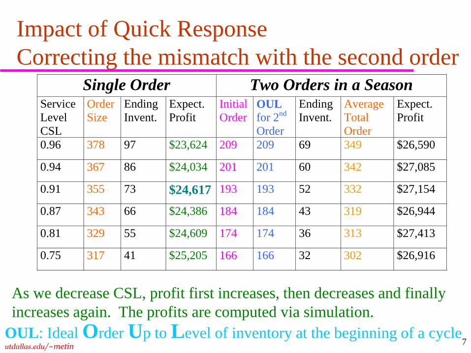
Impact of Quick Response

Correcting the mismatch with the second order Single Order Two Orders in a Season

Service

Level

CSL

Order

Size

Ending

Invent.

Expect.

Profit

Initial

Order

OUL

for 2nd

Order

Ending

Invent.

Average

Total

Order

Expect.

Profit

0.96 378 97 $23,624 209 209 69 349 $26,590

0.94 367 86 $24,034 201 201 60 342 $27,085

0.91 355 73 $24,617 193 193 52 332 $27,154

0.87 343 66 $24,386 184 184 43 319 $26,944

0.81 329 55 $24,609 174 174 36 313 $27,413

0.75 317 41 $25,205 166 166 32 302 $26,916

OUL: Ideal Order Up to Level of inventory at the beginning of a cycle

As we decrease CSL, profit first increases, then decreases and finally

increases again. The profits are computed via simulation.

utdallas.edu/~metin

8

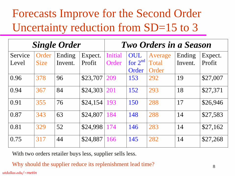
Forecasts Improve for the Second Order

Uncertainty reduction from SD=15 to 3

Single Order Two Orders in a Season Service

Level

Order

Size

Ending

Invent.

Expect.

Profit

Initial

Order

OUL

for 2nd

Order

Average

Total

Order

Ending

Invent.

Expect.

Profit

0.96 378 96 $23,707 209 153 292 19 $27,007

0.94 367 84 $24,303 201 152 293 18 $27,371

0.91 355 76 $24,154 193 150 288 17 $26,946

0.87 343 63 $24,807 184 148 288 14 $27,583

0.81 329 52 $24,998 174 146 283 14 $27,162

0.75 317 44 $24,887 166 145 282 14 $27,268

With two orders retailer buys less, supplier sells less.

Why should the supplier reduce its replenishment lead time?

utdallas.edu/~metin

9

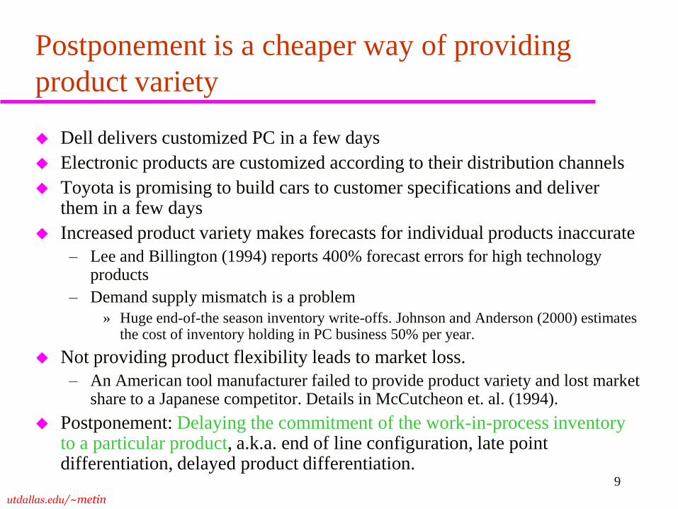
Postponement is a cheaper way of providing

product variety

Dell delivers customized PC in a few days

Electronic products are customized according to their distribution channels

Toyota is promising to build cars to customer specifications and deliver them in a few days

Increased product variety makes forecasts for individual products inaccurate

– Lee and Billington (1994) reports 400% forecast errors for high technology products

– Demand supply mismatch is a problem

» Huge end-of-the season inventory write-offs. Johnson and Anderson (2000) estimates the cost of inventory holding in PC business 50% per year.

Not providing product flexibility leads to market loss.

– An American tool manufacturer failed to provide product variety and lost market share to a Japanese competitor. Details in McCutcheon et. al. (1994).

Postponement: Delaying the commitment of the work-in-process inventory to a particular product, a.k.a. end of line configuration, late point differentiation, delayed product differentiation.

utdallas.edu/~metin 10

Postponement

Postponement is delaying customization step as much as

possible

Need:

– Indistinguishable products/components before customization

– Customization step is high value added

– Unpredictable demand

– Negatively correlated product demands

– Flexible SC to allow for any choice of customization step

utdallas.edu/~metin

11

Forms of Postponement by Zinn and Bowersox (1988)

Labeling postponement: Standard product is labeled

differently based on the realized demand. – HP printer division places labels in appropriate language on to printers after the

demand is observed.

Packaging postponement: Packaging performed at the

distribution center. – In electronics manufacturing, semi-finished goods are transported from SE Asia to

North America and Europe where they are localized according to local language and

power supply

Assembly and manufacturing postponement: Assembly

or manufacturing is done after observing the demand. – McDonalds assembles meal menus after customer order.

utdallas.edu/~metin

12

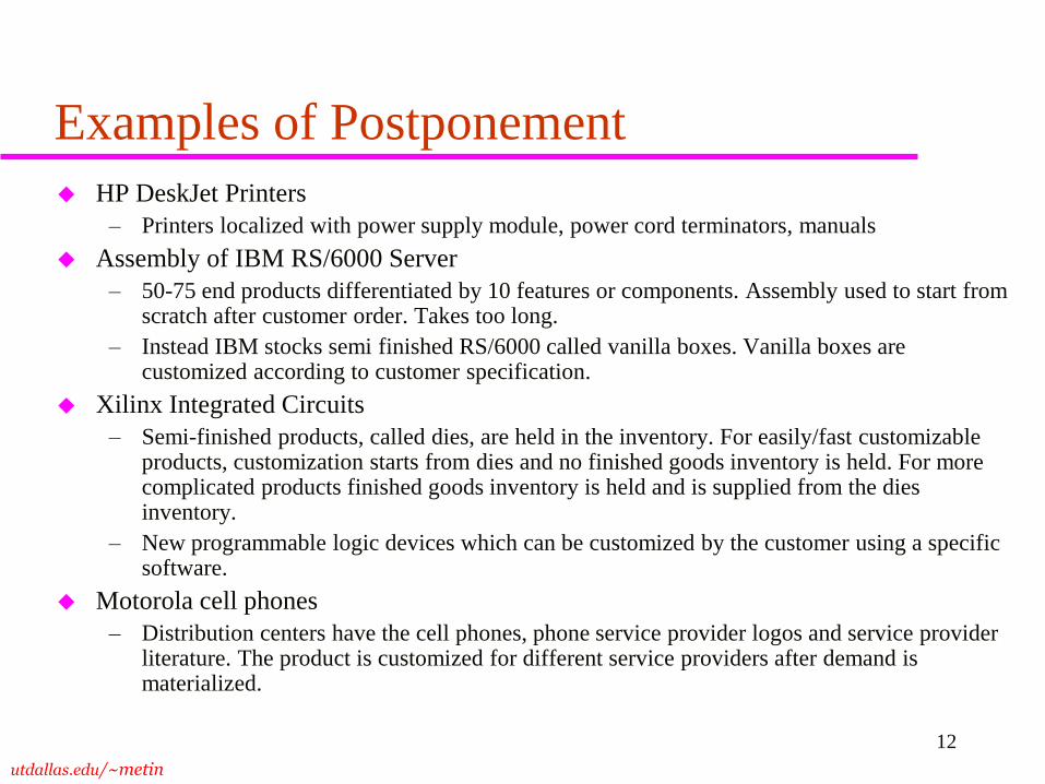
Examples of Postponement

HP DeskJet Printers

– Printers localized with power supply module, power cord terminators, manuals

Assembly of IBM RS/6000 Server

– 50-75 end products differentiated by 10 features or components. Assembly used to start from scratch after customer order. Takes too long.

– Instead IBM stocks semi finished RS/6000 called vanilla boxes. Vanilla boxes are customized according to customer specification.

Xilinx Integrated Circuits

– Semi-finished products, called dies, are held in the inventory. For easily/fast customizable products, customization starts from dies and no finished goods inventory is held. For more complicated products finished goods inventory is held and is supplied from the dies inventory.

– New programmable logic devices which can be customized by the customer using a specific software.

Motorola cell phones

– Distribution centers have the cell phones, phone service provider logos and service provider literature. The product is customized for different service providers after demand is materialized.

utdallas.edu/~metin

13

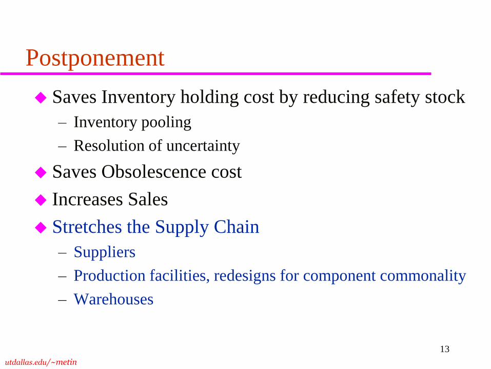
Postponement

Saves Inventory holding cost by reducing safety stock

– Inventory pooling

– Resolution of uncertainty

Saves Obsolescence cost

Increases Sales

Stretches the Supply Chain

– Suppliers

– Production facilities, redesigns for component commonality

– Warehouses

utdallas.edu/~metin

14

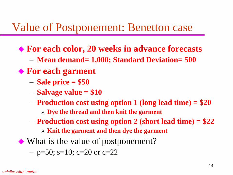
Value of Postponement: Benetton case

For each color, 20 weeks in advance forecasts

– Mean demand= 1,000; Standard Deviation= 500

For each garment

– Sale price = $50

– Salvage value = $10

– Production cost using option 1 (long lead time) = $20

» Dye the thread and then knit the garment

– Production cost using option 2 (short lead time) = $22

» Knit the garment and then dye the garment

What is the value of postponement?

– p=50; s=10; c=20 or c=22

utdallas.edu/~metin

15

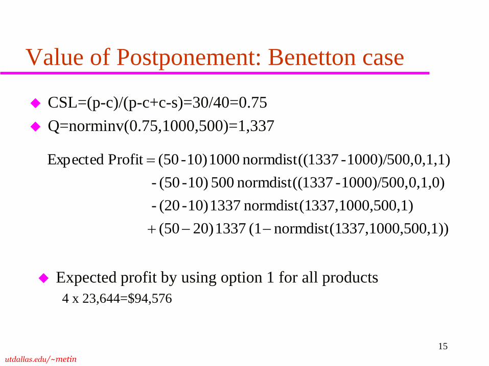
Value of Postponement: Benetton case

CSL=(p-c)/(p-c+c-s)=30/40=0.75

Q=norminv(0.75,1000,500)=1,337

00,1))337,1000,5normdist(1(1 1337 20)(50

00,1)337,1000,5normdist(1 1337 10)-(20 -

0,1,0)1000)/500,-1337normdist(( 500 10)-(50 -

0,1,1)1000)/500,-1337normdist(( 1000 10)-(50 Profit Expected

Expected profit by using option 1 for all products

4 x 23,644=$94,576

utdallas.edu/~metin

16

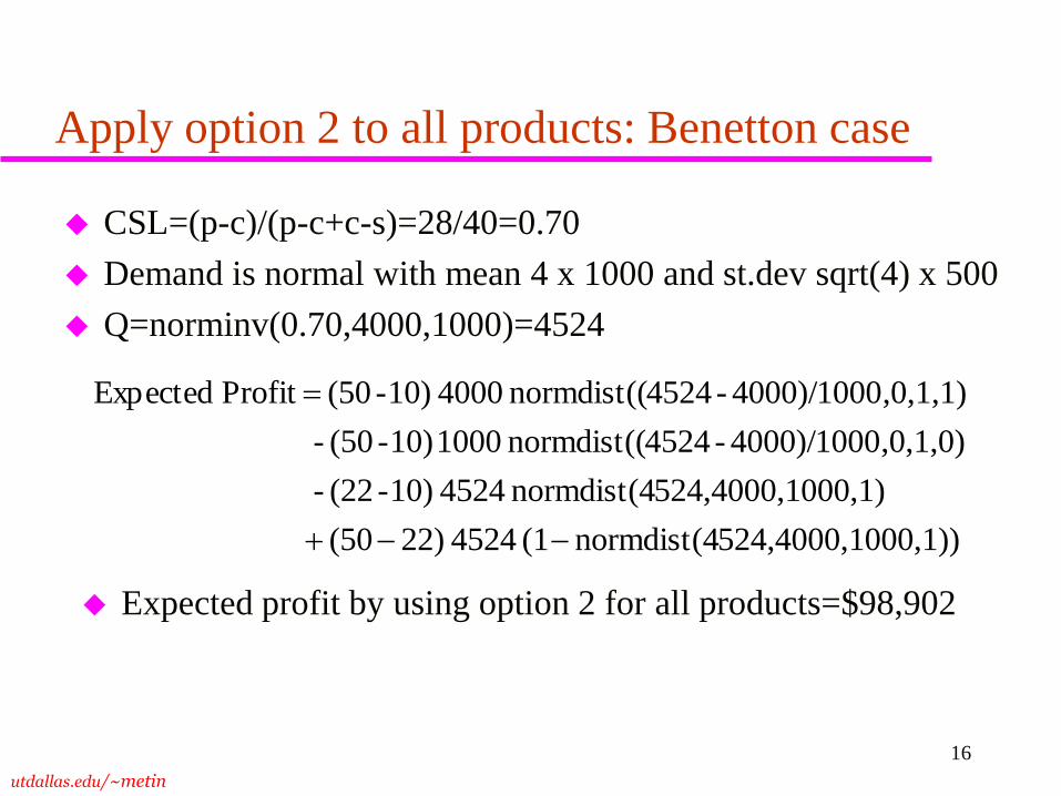
Apply option 2 to all products: Benetton case

CSL=(p-c)/(p-c+c-s)=28/40=0.70

Demand is normal with mean 4 x 1000 and st.dev sqrt(4) x 500

Q=norminv(0.70,4000,1000)=4524

000,1))524,4000,1normdist(4(1 4524 22)(50

000,1)524,4000,1normdist(4 4524 10)-(22 -

,0,1,0)4000)/1000-4524normdist(( 1000 10)-(50 -

,0,1,1)4000)/1000-4524normdist(( 4000 10)-(50 Profit Expected

Expected profit by using option 2 for all products=$98,902

utdallas.edu/~metin

17

Postponement Downside

By postponing all three garment types, production cost

of each product goes up

When this increase is substantial or a single product’s

demand dominates all other’s (causing limited

uncertainty reduction via aggregation), a partial

postponement scheme is preferable to full

postponement.

utdallas.edu/~metin

18

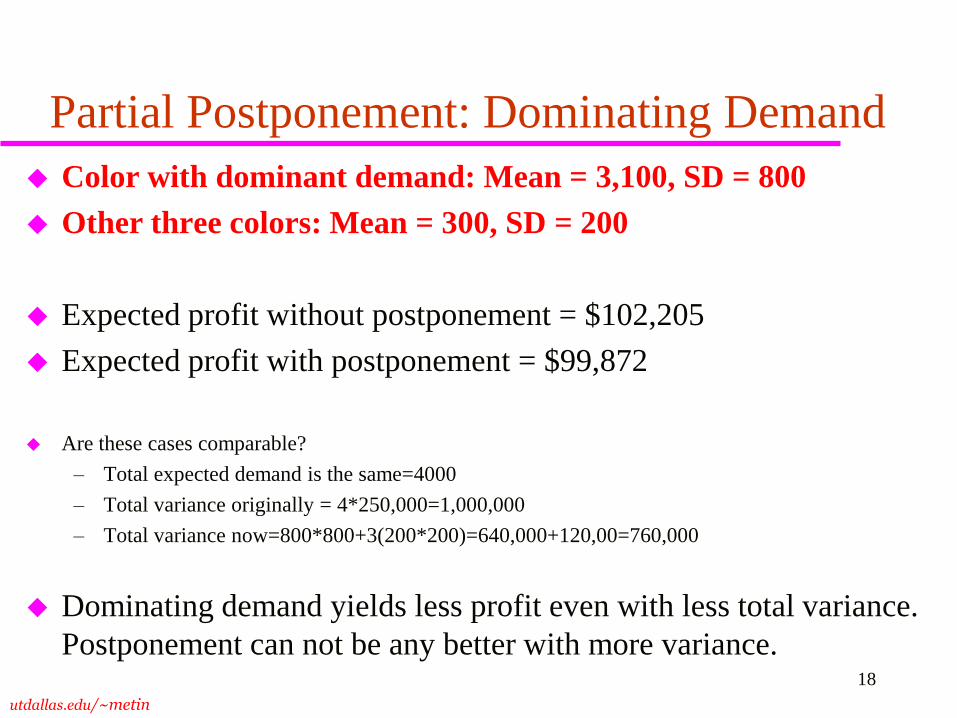
Partial Postponement: Dominating Demand

Color with dominant demand: Mean = 3,100, SD = 800

Other three colors: Mean = 300, SD = 200

Expected profit without postponement = $102,205

Expected profit with postponement = $99,872

Are these cases comparable?

– Total expected demand is the same=4000

– Total variance originally = 4*250,000=1,000,000

– Total variance now=800*800+3(200*200)=640,000+120,00=760,000

Dominating demand yields less profit even with less total variance.

Postponement can not be any better with more variance.

utdallas.edu/~metin

19

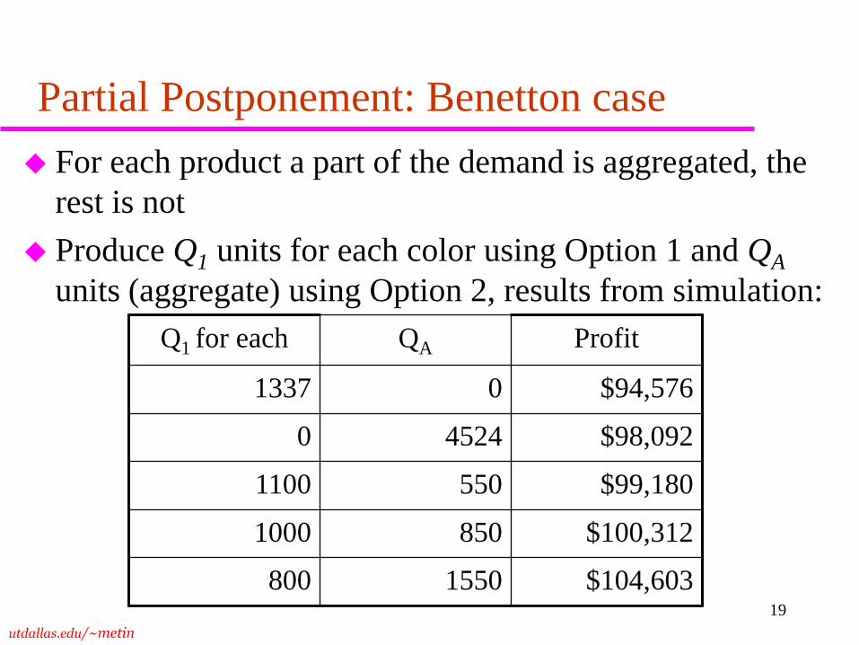
Partial Postponement: Benetton case

For each product a part of the demand is aggregated, the

rest is not

Produce Q1 units for each color using Option 1 and QA

units (aggregate) using Option 2, results from simulation:

Q1 for each QA Profit

1337 0 $94,576

0 4524 $98,092

1100 550 $99,180

1000 850 $100,312

800 1550 $104,603

utdallas.edu/~metin

20

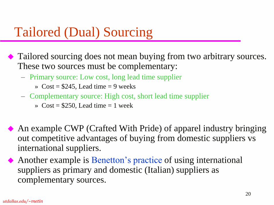
Tailored (Dual) Sourcing

Tailored sourcing does not mean buying from two arbitrary sources. These two sources must be complementary:

– Primary source: Low cost, long lead time supplier

» Cost = $245, Lead time = 9 weeks

– Complementary source: High cost, short lead time supplier

» Cost = $250, Lead time = 1 week

An example CWP (Crafted With Pride) of apparel industry bringing out competitive advantages of buying from domestic suppliers vs international suppliers.

Another example is Benetton’s practice of using international suppliers as primary and domestic (Italian) suppliers as complementary sources.

utdallas.edu/~metin

21

Summary

Levers for improving profitability

– Increase salvage value and decrease cost of stockout

– Improved forecasting

– Quick response with multiple orders

– Postponement

– Tailored sourcing

utdallas.edu/~metin 22

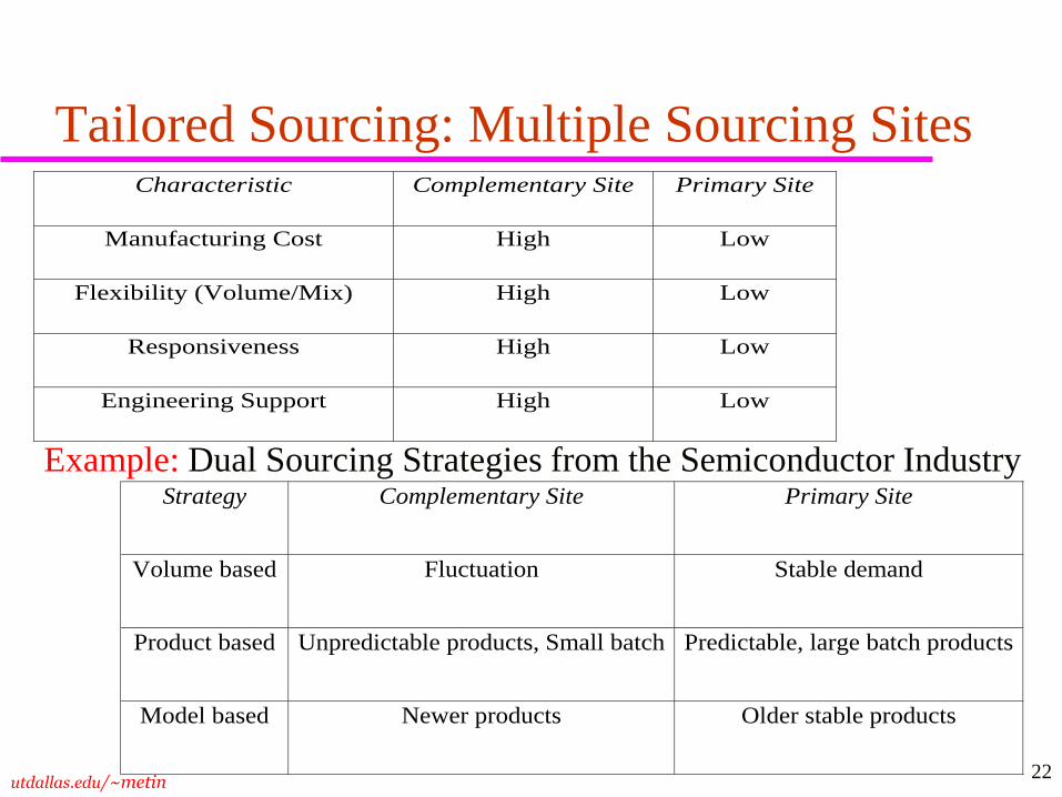
Tailored Sourcing: Multiple Sourcing Sites Characteristic Complementary Site Primary Site

Manufacturing Cost High Low

Flexibility (Volume/Mix) High Low

Responsiveness High Low

Engineering Support High Low

Strategy Complementary Site Primary Site

Volume based Fluctuation Stable demand

Product based Unpredictable products, Small batch Predictable, large batch products

Model based Newer products Older stable products

Example: Dual Sourcing Strategies from the Semiconductor Industry