Embed Size (px)
Citation preview
Leveraging Tripartite Interaction Information from Live StreamE-Commerce for Improving Product Recommendation
Sanshi Yu1∗, Zhuoxuan Jiang
2∗, Dong-Dong Chen
3, Shanshan Feng
4,
Dongsheng Li5, Qi Liu
1, Jinfeng Yi
3
1University of Science and Technology of China, Hefei, China
2Tencent, Shanghai, China
3JD AI Research, Beijing, China
4Harbin Institute of Technology, Shenzhen, China
5Microsoft Research Asia, Shanghai, China
[email protected],[email protected],{chendongdong1,yijinfeng}@jd.com,
[email protected],[email protected],[email protected]
ABSTRACTRecently, a new form of online shopping becomes more and more
popular, which combines live streaming with E-Commerce activity.
The streamers introduce products and interact with their audiences,
and hence greatly improve the performance of selling products.
Despite of the successful applications in industries, the live stream E-
commerce has not been well studied in the data science community.
To fill this gap, we investigate this brand-new scenario and collect
a real-world Live Stream E-Commerce (LSEC) dataset. Different
from conventional E-commerce activities, the streamers play a
pivotal role in the LSEC events. Hence, the key is to make full
use of rich interaction information among streamers, users, and
products. We first conduct data analysis on the tripartite interaction
data and quantify the streamer’s influence on users’ purchase
behavior. Based on the analysis results, we model the tripartite
information as a heterogeneous graph, which can be decomposed to
multiple bipartite graphs in order to better capture the influence.We
propose a novel Live Stream E-Commerce Graph Neural Network
framework (LSEC-GNN) to learn the node representations of each
bipartite graph, and further design a multi-task learning approach
to improve product recommendation. Extensive experiments on
two real-world datasets with different scales show that our method
can significantly outperform various baseline approaches.
CCS CONCEPTS• Information systems→ Recommender systems; • Comput-ing methodologies → Learning latent representations.
KEYWORDSgraph representation learning; multi-task learning; live streaming
E-Commence; product recommendation
Permission to make digital or hard copies of all or part of this work for personal or
classroom use is granted without fee provided that copies are not made or distributed
for profit or commercial advantage and that copies bear this notice and the full citation
on the first page. Copyrights for components of this work owned by others than ACM
must be honored. Abstracting with credit is permitted. To copy otherwise, or republish,
to post on servers or to redistribute to lists, requires prior specific permission and/or a
fee. Request permissions from [email protected].
KDD ’21, August 14–18, 2021, Virtual Event, Singapore.© 2021 Association for Computing Machinery.
ACM ISBN 978-1-4503-8332-5/21/08. . . $15.00
https://doi.org/10.1145/3447548.3467151
ACM Reference Format:Sanshi Yu
1[1], Zhuoxuan Jiang
2[1], Dong-Dong Chen
3, Shanshan Feng
4,,
Dongsheng Li5, Qi Liu
1, Jinfeng Yi
3. 2021. Leveraging Tripartite Inter-
action Information from Live Stream E-Commerce for Improving Prod-
uct Recommendation. In Proceedings of the 27th ACM SIGKDD Confer-ence on Knowledge Discovery and Data Mining (KDD ’21), August 14–18,2021, Virtual Event, Singapore. ACM, New York, NY, USA, 9 pages. https:
//doi.org/10.1145/3447548.3467151
1 INTRODUCTIONRecent years witness the prosperity of online live streaming. With
the development of mobile phones, cameras, and high-speed inter-
net, more and more users are able to broadcast their experiences in
live streams on various social platforms, such as Facebook Live and
YouTube Live. There are a variety of live streaming applications [19],
including knowledge share, video-gaming, and outdoor traveling.
One of the most important scenarios is live streaming commerce,
where streamers broadcast themselves online and promote products
to their audiences, as shown in Figure 1.
This new form of sales can greatly shorten the decision-making
time of consumers and provoke the sales volume [1, 10]. For ex-
ample, according to a report from Alibaba’s Taobao Live platform,
there are several numbers worthy of attention in last year’s 11.11
Global Shopping Festival: (1) the total GMV driven by live streaming
achieved $6 Billion USD, (2) approximately 300 million Taobao users
watched live streams, and (3) 33 live streaming channels achieved
over $15million USD in sales and nearly 500 live streaming channels
reached $1.5 million USD [4]. Some quantitative research results
show that adopting live streaming in sales can achieve a 21.8%
increase in online sales volume [1].
This new kind of shopping experience is significantly different
from conventional online shopping, where only static informa-
tion, e.g., images and texts, are available for customers. The expert
streamers introduce and promote the products in a live streaming
manner, which makes the shopping process more interesting and
convincing. In addition, another feature of live streaming is the rich
and real-time interactions between streamers and their audiences,
which makes live streaming a new medium and a powerful market-
ing tool for E-Commerce. Compared with the traditional TV live
∗The authors contributed equally to this work, which was done when they were in JD
AI Research and Sanshi Yu was an intern. Zhuoxuan Jiang and Shanshan Feng are the
corresponding authors.
arX
iv:2
106.
0341
5v1
[cs
.IR
] 7
Jun
202
1
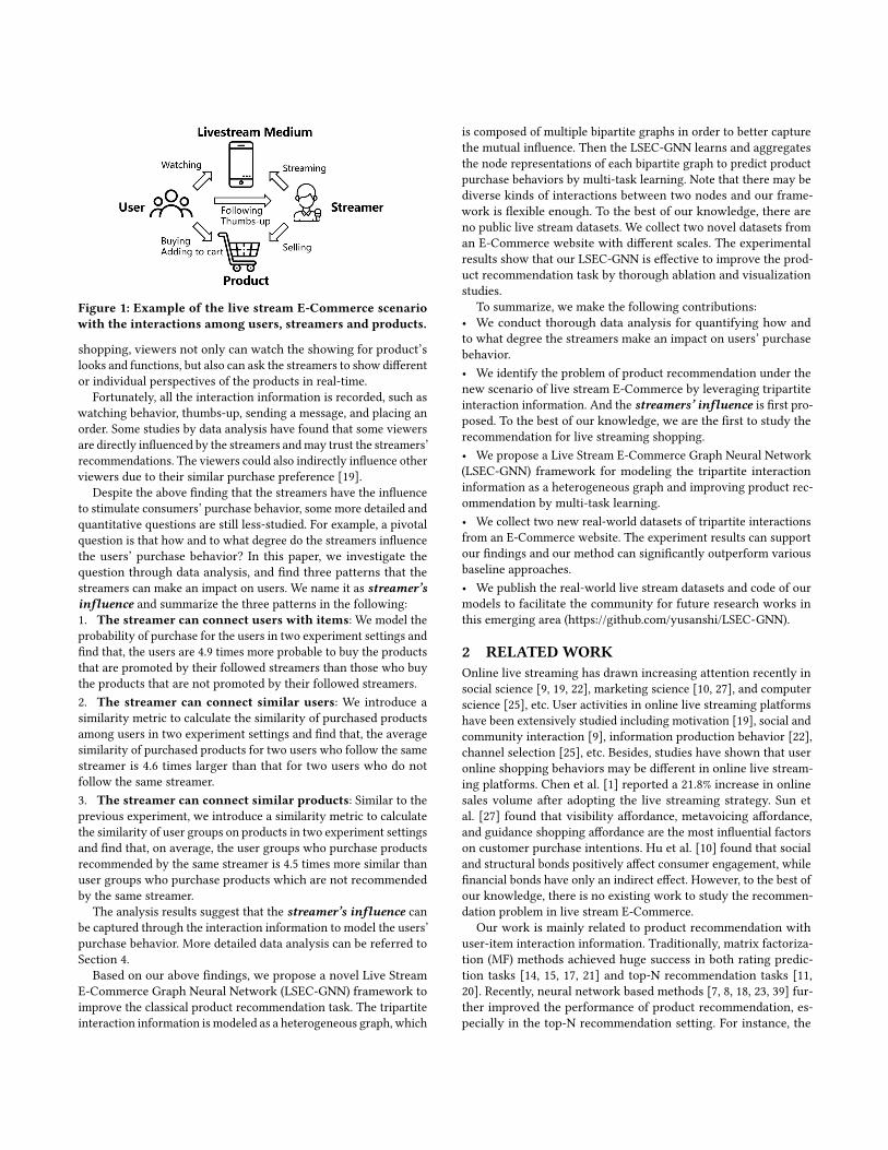
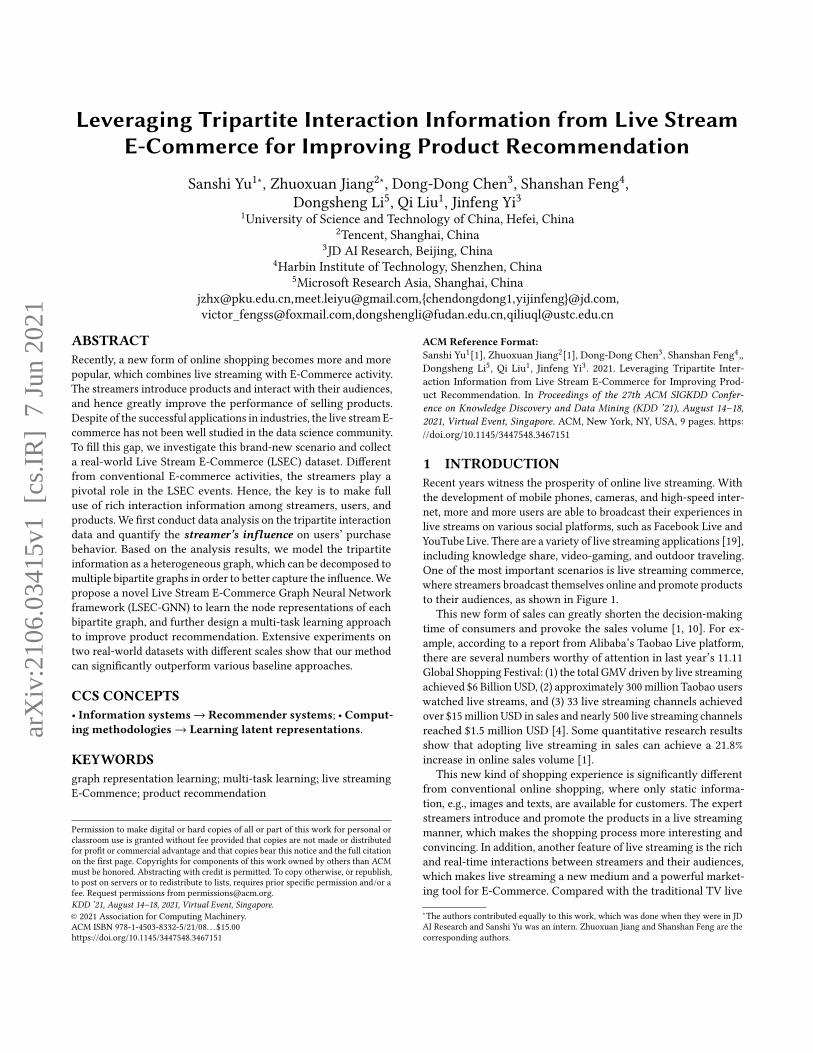
Figure 1: Example of the live stream E-Commerce scenariowith the interactions among users, streamers and products.
shopping, viewers not only can watch the showing for product’s
looks and functions, but also can ask the streamers to show different
or individual perspectives of the products in real-time.
Fortunately, all the interaction information is recorded, such as
watching behavior, thumbs-up, sending a message, and placing an
order. Some studies by data analysis have found that some viewers
are directly influenced by the streamers andmay trust the streamers’
recommendations. The viewers could also indirectly influence other
viewers due to their similar purchase preference [19].
Despite the above finding that the streamers have the influence
to stimulate consumers’ purchase behavior, some more detailed and
quantitative questions are still less-studied. For example, a pivotal
question is that how and to what degree do the streamers influence
the users’ purchase behavior? In this paper, we investigate the
question through data analysis, and find three patterns that the
streamers can make an impact on users. We name it as streamer’sinfluence and summarize the three patterns in the following:
1. The streamer can connect users with items: We model the
probability of purchase for the users in two experiment settings and
find that, the users are 4.9 times more probable to buy the products
that are promoted by their followed streamers than those who buy
the products that are not promoted by their followed streamers.
2. The streamer can connect similar users: We introduce a
similarity metric to calculate the similarity of purchased products
among users in two experiment settings and find that, the average
similarity of purchased products for two users who follow the same
streamer is 4.6 times larger than that for two users who do not
follow the same streamer.
3. The streamer can connect similar products: Similar to the
previous experiment, we introduce a similarity metric to calculate
the similarity of user groups on products in two experiment settings
and find that, on average, the user groups who purchase products
recommended by the same streamer is 4.5 times more similar than
user groups who purchase products which are not recommended
by the same streamer.
The analysis results suggest that the streamer’s influence canbe captured through the interaction information to model the users’
purchase behavior. More detailed data analysis can be referred to
Section 4.
Based on our above findings, we propose a novel Live Stream
E-Commerce Graph Neural Network (LSEC-GNN) framework to
improve the classical product recommendation task. The tripartite
interaction information is modeled as a heterogeneous graph, which
is composed of multiple bipartite graphs in order to better capture
the mutual influence. Then the LSEC-GNN learns and aggregates
the node representations of each bipartite graph to predict product
purchase behaviors by multi-task learning. Note that there may be
diverse kinds of interactions between two nodes and our frame-
work is flexible enough. To the best of our knowledge, there are
no public live stream datasets. We collect two novel datasets from
an E-Commerce website with different scales. The experimental
results show that our LSEC-GNN is effective to improve the prod-
uct recommendation task by thorough ablation and visualization
studies.
To summarize, we make the following contributions:
• We conduct thorough data analysis for quantifying how and
to what degree the streamers make an impact on users’ purchase
behavior.
• We identify the problem of product recommendation under the
new scenario of live stream E-Commerce by leveraging tripartite
interaction information. And the streamers’ influence is first pro-posed. To the best of our knowledge, we are the first to study the
recommendation for live streaming shopping.
• We propose a Live Stream E-Commerce Graph Neural Network
(LSEC-GNN) framework for modeling the tripartite interaction
information as a heterogeneous graph and improving product rec-
ommendation by multi-task learning.
• We collect two new real-world datasets of tripartite interactions
from an E-Commerce website. The experiment results can support
our findings and our method can significantly outperform various
baseline approaches.
• We publish the real-world live stream datasets and code of our
models to facilitate the community for future research works in
this emerging area (https://github.com/yusanshi/LSEC-GNN).
2 RELATEDWORKOnline live streaming has drawn increasing attention recently in
social science [9, 19, 22], marketing science [10, 27], and computer
science [25], etc. User activities in online live streaming platforms
have been extensively studied including motivation [19], social and
community interaction [9], information production behavior [22],
channel selection [25], etc. Besides, studies have shown that user
online shopping behaviors may be different in online live stream-
ing platforms. Chen et al. [1] reported a 21.8% increase in online
sales volume after adopting the live streaming strategy. Sun et
al. [27] found that visibility affordance, metavoicing affordance,
and guidance shopping affordance are the most influential factors
on customer purchase intentions. Hu et al. [10] found that social
and structural bonds positively affect consumer engagement, while
financial bonds have only an indirect effect. However, to the best of
our knowledge, there is no existing work to study the recommen-
dation problem in live stream E-Commerce.
Our work is mainly related to product recommendation with
user-item interaction information. Traditionally, matrix factoriza-
tion (MF) methods achieved huge success in both rating predic-
tion tasks [14, 15, 17, 21] and top-N recommendation tasks [11,
20]. Recently, neural network based methods [7, 8, 18, 23, 39] fur-
ther improved the performance of product recommendation, es-
pecially in the top-N recommendation setting. For instance, the
NCF method [7] improved the traditional MF methods by intro-
ducing MLPs to model the non-linear interactions between users
and items. Similarly, many advanced neural network methods were
applied in recommendation tasks to further enhance the state-of-
the-art performance, e.g., autoencoders [18, 23], recurrent neural
networks [8, 39], etc. More recently, graph neural networks were
introduced to the many recommendation tasks, which can improve
the performance by combining both user rating information and
the user-item interaction graph information [2, 6, 16, 28, 30, 37,
38, 43, 44]. However, these GNN based methods were focused on
bipartite graphs, which may not be optimal for tripartite graphs in
product recommendation problem of live stream E-Commerce.
Similar to this work, many existing works incorporated addi-
tional graphs beside the user-item interaction graphs in recom-
mendation tasks, e.g., knowledge graphs [24, 33, 34, 36] and social
graphs [3, 26, 40–42]. For instance, Wang et al. [33] proposed the
knowledge-aware graph neural network with label smoothness
regularization, which first applies a trainable function to identify
important KG relationships and then applies a GNN to compute
personalized item embeddings. Wang et al. [36] proposed the KGAT
method, which can capture the high-order relations from the hybrid
structure of KG and user-item graph via attention mechanism. Wu
et al. [41] proposed a dual graph attention network to collabora-
tively learn user/item representations via a user-specific attention
weight and a context-aware attention weight for a more accurate so-
cial recommendation. Fan et al. [3] proposed the GraphRec method,
which can jointly capture interactions and opinions in the user-
item interaction graph and consider heterogeneous strengths of
social relations. Our work is orthogonal to the above works, i.e.,
the proposed method can be adopted to improve their performance
if they are applied in the product recommendation problem of live
stream E-Commerce.
3 PROBLEM DEFINITIONIn this section, we define the problem of product recommendation
in live streaming E-Commerce by modeling tripartite interaction
information. Different from the conventional E-Commerce recom-
mendation methods that only leverage the bipartite interactions
between users and items, we have the tripartite relationship in the
targeted problem. The basic idea is to incorporate all the three kinds
of bipartite interaction information, model the message propaga-
tion process and jointly learn the three tasks. To achieve this, it
is desirable to first model the different kinds of interaction infor-
mation as bipartite graphs and learn the unified representation to
encode the tripartite entities. In this paper, we propose three bipar-
tite graphs to model different interaction information, including
user-item interaction graph, streamer-item interaction graph, and
streamer-user interaction graph.
Definition 1. (User-Item Graph) User-item graph, denoted
as G(𝑢,𝑖) = (U ∪ I, E (𝑢,𝑖 ), captures the interaction information
between users and items, and the interaction means users buy the
corresponding items. U is a set of users and I is a set of items.
E (𝑢,𝑖) is the set of edges between users and items. We set the edge
weight𝑤 (𝑢,𝑖) 𝑗𝑘as 1 if user 𝑢 𝑗 buys item 𝑖𝑘 , otherwise 0. The user-
item graph directly captures the interaction relationship between
users and products, which is the essential information used by
existing product recommendation approaches such as NGCF [37].
Beyond this kind of interaction information, streamers bring
another two kinds of interactions which can benefit the product rec-
ommendation. The streamer-item graph and streamer-user graph
are defined as below:
Definition 2. (Streamer-Item Graph) Streamer-item graph,
denoted as G(𝑠,𝑖) = (S ∪ I, E (𝑠,𝑖 ), is a bipartite graph where S is
a set of streamers and I is a set of items. E (𝑠,𝑖 ) is the set of edgesbetween streamers and items. The edge weight𝑤
(𝑠,𝑖)𝑗𝑘
is set as 1 if
the streamer 𝑠 𝑗 sells item 𝑖𝑘 , otherwise 0.
The user-item graph and streamer-item graph capture the inter-
action information between humans and products from different
perspectives. The user-item graph encodes the buying relation,
while the stream-item graph encodes the selling relation. To en-
code the following relation between streamers and users, we in-
troduce the streamer-user graph, which captures the interaction
between humans.
Definition 3. (Streamer-User Graph) Streamer-user graph,
denoted as G(𝑠,𝑢) = (S ∪U, E (𝑠,𝑢 ), is a bipartite graph where S is
a set of streamers and U is a set of users. E (𝑠,𝑢 ) is the set of edgesbetween streamers and users. The edge weight𝑤
(𝑠,𝑢)𝑗𝑘
is set as 1 if
the streamer 𝑠 𝑗 is followed by user 𝑢𝑘 , otherwise 0.
These three types of graphs can be further integrated into one
heterogeneous interaction graph.
Definition 4. (Heterogeneous Tripartite Interaction Graph)The heterogeneous tripartite interaction graph is the combination
of user-item, streamer-item, and streamer-user graphs constructed
from three kinds of entities (user, item, and streamer) with their
multi-view historical interaction data. It captures tripartite per-
spectives of interaction relationship between humans and products
specifically in live stream E-Commerce.
Note that the definition of a heterogeneous tripartite interaction
graph can be generalized to integrate other types of interaction
graphs such as adding to cart relation between users and items, and
watching relation between streamers and users. In this work we
are using the three types of interaction graphs (buying, selling and
following) as an illustrative example, which are much related to
the product recommendation task.
Finally, we formally define the problem of product recommenda-
tion by modeling tripartite interaction information as follows:
Definition 5. Product Recommendation with Tripartite In-teraction Information Given a large collection of interaction data
between users, products, and streamers in live stream E-Commerce
scenarios, the problem of product recommendation with tripartite
interaction information aims to learn and aggregate low-dimensional
representations of tripartite nodes by embedding the heterogeneous
interaction graph and then make recommendations based on the
learned representations by multi-task prediction.
4 DATA ANALYSISBefore proposing the solution for product recommendation in live
stream E-Commerce, in this section, we show the correlation be-
tween streamers and users’ purchase by data analysis. As shown
in Figure 2, there are three patterns among users and items by
Figure 2: Examples of three different patterns that streamerscouldmake an impact onusers’ purchase behavior. The solidlines mean the observed interaction behaviors and the dashlines mean the potential purchase behaviors.
introducing streamers as mediums: (a) The streamer can connect
users with items, (b) The streamer can connect similar users, (c) The
streamer can connect similar products. We put forward three ques-
tions corresponding to the three patterns respectively and present
the detailed analysis to answer these questions.
4.1 Relation Pattern between Users and ItemsThis pattern means that the streamer acts as a bridge to connect
the user and the item. In this relationship, we aim to answer:
• Whether there is a higher probability of purchase for the usersfacing the items sold by their following streamers?We conduct a simulation experiment by theMonte Carlomethod [29]
to calculate the probability of purchase for the users in two settings.
The first setting 𝑆1 is that the users are presented with items sold
by their following streamers, while the second setting 𝑆2 is that the
users are presented with items which are not sold by their following
streamers. We utilize set 𝑃 to denote the result in the first setting
and set𝑄 to denote the result in the second setting. The simulation
process is described as :
1. Initialize 𝑃 = ∅ and 𝑄 = ∅.2. Sample a user and an item randomly.
3. Set 𝑡 = 1 if the user purchases the item, otherwise set 𝑡 = 0.
4. Put 𝑡 into 𝑃 for the first setting or 𝑄 for the second setting.
5. Repeat (2)-(4) for 𝑁𝑀𝐶 times.
Here, 𝑁𝑀𝐶 is a large number of Monte Carlo simulations to ensure
both |𝑃 | and |𝑄 | are comparable to the total number of the interac-
tions between users and items. The probability of user purchasing
items in the first setting 𝑆1 can be calculated as follows:
𝑃𝑟𝑜𝑏1 =𝑃𝑠𝑢𝑚
|𝑃 | , (1)
where 𝑃𝑠𝑢𝑚 denotes the sum of occurred purchases in set 𝑃 . Sim-
ilarly, We can also get the probability of user purchase items in
the second setting 𝑆2 by replacing 𝑃 with 𝑄 in the Equation 1. We
run the experiments for 5 times and report the average results in
Table 1. We observe that the user purchasing probability of items
sold by his/her following streamers is approximately 5 times of
those not sold by the streamers. The analysis result indicates that
the User-Streamer-Item pattern can help to enhance the purchase
probability between users and items, as shown in Figure 2(a).
4.2 Relation Pattern between UsersThis pattern indicates that the streamer acts as a bridge to connect
two users. In this pattern, we aim to answer:
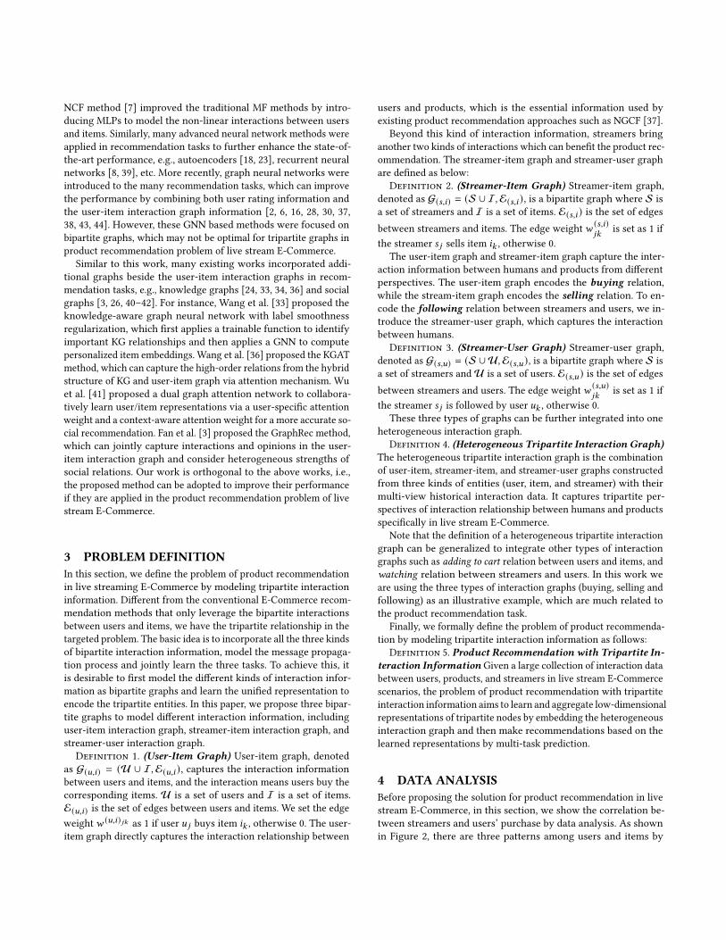
Table 1: The results of the simulation experiments.
Setting Probability of purchase (avg ± std)𝑆1 3.35e-4 ± 3.74e-7𝑆2 7.04e-5 ± 1.77e-7
Table 2: The quantiles and mean value of 𝐶𝑜𝑠 𝑗𝑘 and 𝐽𝑎𝑐 𝑗𝑘 inU𝑝𝑎𝑖𝑟
𝑦 andU𝑝𝑎𝑖𝑟𝑛 .
Quantile Level 50% 75% 90% 99% Average𝐶𝑜𝑠 𝑗𝑘 in U𝑝𝑎𝑖𝑟
𝑛 0.0 0.0 0.035 0.22 0.012
𝐶𝑜𝑠 𝑗𝑘 in U𝑝𝑎𝑖𝑟𝑦 0.0 0.088 0.177 0.447 0.055
𝐽 𝑎𝑐 𝑗𝑘 in U𝑝𝑎𝑖𝑟𝑛 0.0 0.0 0.0156 0.10 0.0055
𝐽 𝑎𝑐 𝑗𝑘 in U𝑝𝑎𝑖𝑟𝑦 0.0 0.0385 0.0769 0.25 0.0259
Table 3: The quantiles and mean value of 𝐶𝑜𝑠 𝑗𝑘 and 𝐽𝑎𝑐 𝑗𝑘 inI𝑝𝑎𝑖𝑟𝑦 and I𝑝𝑎𝑖𝑟
𝑛 .
Quantile Level 98% 99% 99.9% 99.99% Average𝐶𝑜𝑠 𝑗𝑘 in I𝑝𝑎𝑖𝑟
𝑛 0.0 0.0 0.031 0.10 8.7e-5
𝐶𝑜𝑠 𝑗𝑘 in I𝑝𝑎𝑖𝑟𝑦 0.0 0.01 0.072 0.18 3.9e-4
𝐽 𝑎𝑐 𝑗𝑘 in I𝑝𝑎𝑖𝑟𝑛 0.0 0.0 0.011 0.044 3.5e-5
𝐽 𝑎𝑐 𝑗𝑘 in I𝑝𝑎𝑖𝑟𝑦 0.0 0.003 0.029 0.098 1.59e-4
• When two users follow the same streamer, will their purchaseditems be more similar?Here, we utilize Cosine similarity and Jaccard similarity coeffi-
cient [12] to measure the similarity between two item sets pur-
chased by two users. For calculating the Cosine similarity 𝐶𝑜𝑠 𝑗𝑘between user 𝑢 𝑗 and 𝑢𝑘 , we represent 𝑢 𝑗 with a 𝑁 -dimensional
vector 𝑣𝑢𝑗, in which the 𝑛-th dimension is 1 if 𝑢 𝑗 purchases the 𝑛-th
item and 0 otherwise. The Cosine similarity𝐶𝑜𝑠 𝑗𝑘 can be calculated:
𝐶𝑜𝑠 𝑗𝑘 =
⟨𝑣𝑢𝑗, 𝑣𝑢𝑘
⟩|𝑣𝑢𝑗| ∗ |𝑣𝑢
𝑘| . (2)
The Jaccard similarity coefficient 𝐽𝑎𝑐 𝑗𝑘 between user 𝑢 𝑗 and 𝑢𝑘 can
be calculated as follows:
𝐽𝑎𝑐 𝑗𝑘 =|I𝑗 ∩ I𝑘 ||I𝑗 ∪ I𝑘 |
, (3)
where I𝑗 denotes the item set purchased by user 𝑢 𝑗 and I𝑘 denotes
the item set purchased by user 𝑢𝑘 . We use U𝑝𝑎𝑖𝑟𝑦 to denote the
set of user pairs where two users follow the same streamer, and
useU𝑝𝑎𝑖𝑟𝑛 to denote the set of user pairs where two users do not
follow the same streamer. In order to study the distribution of the
𝐶𝑜𝑠 𝑗𝑘 and 𝐽𝑎𝑐 𝑗𝑘 inU𝑝𝑎𝑖𝑟𝑦 andU𝑝𝑎𝑖𝑟
𝑛 , we randomly sample multiple
pairs from the set U𝑝𝑎𝑖𝑟𝑦 and U𝑝𝑎𝑖𝑟
𝑛 respectively and calculate
𝐶𝑜𝑠 𝑗𝑘 and 𝐽𝑎𝑐 𝑗𝑘 for them. The statistical information (quantiles
and mean value) of the𝐶𝑜𝑠 𝑗𝑘 and 𝐽𝑎𝑐 𝑗𝑘 for two sets are reported in
Table 2.We can learn that𝐶𝑜𝑠 𝑗𝑘 and 𝐽𝑎𝑐 𝑗𝑘 inU𝑝𝑎𝑖𝑟𝑦 are significantly
greater than those in U𝑝𝑎𝑖𝑟𝑛 on the quantiles and mean value. The
result demonstrates that when two users follow the same streamer,
they are more likely to purchase similar items. This experimental
analysis indicates that the User-Streamer-User relationship can
help to learn user similarities, which is beneficial to recommend
items to similar users as illustrated in Figure 2(b).

4.3 Relation Pattern between ItemsThis pattern means that the streamer acts as a bridge to connect
two items. In this relationship, we aim to answer:
• When two items are sold by the same streamer, will the purchasersbetween them be more similar?We also adopt the Cosine similarity and the Jaccard similarity coef-
ficient to represent the similarity between two user sets. For the
Cosine similarity, we represent 𝑖 𝑗 with a 𝑀-dimensional vector 𝑣𝑖𝑗
in which the 𝑚-th dimension is 1 if 𝑖 𝑗 is purchased by the 𝑚-th
user and 0 otherwise. We use U𝑘 to denote the set of users who
purchased the item 𝑖𝑘 and use U𝑗 to denote the set of users who
purchased the item 𝑖 𝑗 . The Jaccard similarity coefficient 𝐽𝑎𝑐𝑘 𝑗 be-
tweenU𝑘 andU𝑗 can also be calculated by Equation 3. Similarly,
we use I𝑝𝑎𝑖𝑟𝑦 to denote the set of item pairs, where each pair rep-
resents that two items are sold by the same streamer. We utilize
I𝑝𝑎𝑖𝑟𝑛 to denote the set of item pairs where two items are not sold
by the same streamer.
The statistical information (quantiles and mean value) of the
𝐶𝑜𝑠 𝑗𝑘 and 𝐽𝑎𝑐 𝑗𝑘 for I𝑝𝑎𝑖𝑟𝑦 and I𝑝𝑎𝑖𝑟
𝑛 are shown in Table 3. Note
that the quantity of an item being purchased by users is much
larger than the quantity of a user purchasing items. Hence, the
similarities in I𝑝𝑎𝑖𝑟𝑦 and I𝑝𝑎𝑖𝑟
𝑛 are much smaller than those in
U𝑝𝑎𝑖𝑟𝑦 andU𝑝𝑎𝑖𝑟
𝑛 . Therefore, we set a larger quantile level in this
analysis. The results in Table 3 show that the Jaccard similarity
coefficient and Cosine similarity in I𝑝𝑎𝑖𝑟𝑦 are greater than those in
I𝑝𝑎𝑖𝑟𝑛 on both the quantiles and mean value, which indicates that
two items sold by the same streamer are more similar. As shown
in Figure 2(c), the analysis in this experiment indicates that the
Item-Streamer-Item pattern can help to identify similar items for
recommendation.
5 METHODOLOGYBased on the previous analysis results, we introduce the details of
the proposed LSEC-GNN framework, in which we perform graph
representation learning by modeling tripartite interaction informa-
tion from live stream E-Commerce to improve product recommen-
dation. Our method first learns vector representations of tripartite
nodes (users, items and streamers) by embedding the heteroge-
neous interaction graphs constructed from interaction data into a
low dimensional space, and then the final node representations are
concatenated from different bipartite graphs. At last, the final node
representations are used to make predictions for multiple tasks.
The overall architecture of LSEC-GNN is illustrated in figure 3.
5.1 Bipartite Graph EmbeddingSince the heterogeneous tripartite interaction graph is composed
of different bipartite graphs with the same node structure, here
we do not distinguish them and introduce the consistent method.
We first build the embedding lookup table for each node in the
heterogeneous interaction graph as follows:
E𝑈 = [𝑒 (0)𝑢1, 𝑒
(0)𝑢2, · · · , 𝑒 (0)𝑢 |U| ] .
E𝐼 = [𝑒 (0)𝑖1, 𝑒
(0)𝑖2, · · · , 𝑒 (0)
𝑖 |I |] .
E𝑆 = [𝑒 (0)𝑠1 , 𝑒(0)𝑠2 , · · · , 𝑒
(0)𝑠 |S| ] .
(4)
The lookup table is shared among bipartite graphs. Then in each
bipartite graph, multiple embedding propagation layers are op-
erated, which refines a node’s representation by aggregating the
embeddings of the interacted nodes. We do not limit the choice of
propagation layers here and one can select any message-passing
aggregator, such as GCN [13], GAT [32], NGCF [37], etc. Take GCN
as the example, the 𝑙-th layer is updated as follows:
𝐻 (𝑙+1) = 𝜎(�̃�− 1
2 �̃��̃�− 1
2𝐻 (𝑙)𝑊 (𝑙))
(5)
where �̃� = 𝐴 + 𝐼𝑁 is the adjacency matrix of a bipartite graph
G with added self-connections. 𝐼𝑁 denotes the identity matrix,
�̃�𝑖𝑖 =∑
𝑗 �̃�𝑖 𝑗 , and𝑊(𝑙)
is a layer-specific trainable weight matrix.
𝜎 (·) denotes the activation function. 𝐻 (𝑙)is the input embeddings
in 𝑙-th layer.
Take the user-item bipartite graph of Figure 3 as an example,
𝑒𝑙−11,𝑢1
means the 𝑢1’s embedding of the (𝑙 − 1)-th layer in the 1-st
bipartite graph,𝑊(𝑙)1,2
means the 2-nd𝑊 in the 1-st bipartite graph.
Note that ideally our framework could model unlimited number of
bipartite graphs. The input embedding 𝐻 (0)and adjacency matrix
𝐴 can be formulated as follows
𝐻 (0) = [E𝑈 , E𝐼 ] .
𝐴 =
[0 𝐴𝑢𝑖𝐴⊺𝑢𝑖
0
].
(6)
Here 𝐴𝑢𝑖 is the user-item interaction matrix. At last after the graph
operations, we can obtain the final representations of each node
from corresponding bitpartite graphs.
5.2 Interaction Graph EmbeddingIn the heterogeneous tripartite interaction graph, where there are
three bipartite graphs, each node of any type will have two embed-
dings from its belonging two bipartite graphs. After GNN opera-
tions, we can concatenate the outputs from each bipartite graph to
generate the final representations of the tripartite nodes as follows:
𝑒∗𝑖 = [𝑒 (𝑁 )1,𝑖
, 𝑒(𝑁 )2,𝑖
]
𝑒∗𝑢 = [𝑒 (𝑁 )1,𝑢
, 𝑒(𝑁 )3,𝑢
]
𝑒∗𝑠 = [𝑒 (𝑁 )2,𝑠
, 𝑒(𝑁 )3,𝑠
]
(7)
Then the final node representations are used for the following
multiple predict tasks.
5.3 Model PredictionAfter generating the unified embedding for each node from the
heterogeneous tripartite interaction graph, we use the embeddings
to make predictions about the existence of edges. Take a user𝑢 as an
example, we denote its embedding learned from user-item-buyingbipartite graph as 𝑣𝑢,buy and the embedding from user-streamer-following as 𝑣𝑢,follow. As the model training, the two embedding
spaces should be close but the distance does exist. For item 𝑖 , we
denote its embedding learned from user-item-buying bipartite graphas 𝑣𝑖,buy and the embedding from streamer-item-selling as 𝑣𝑖,sell.
Now making a prediction based on the unified embedding of 𝑢 and
𝑖 will involve the interaction between totally three vector space,
i.e., the vector spaces of three bipartite graphs. If we take the inner
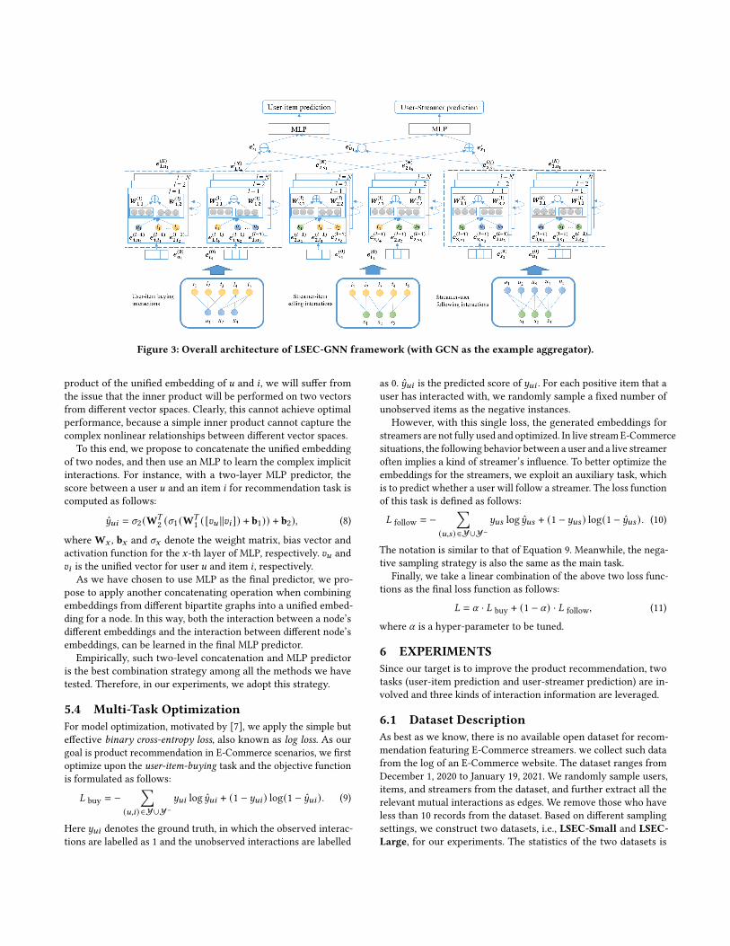
Figure 3: Overall architecture of LSEC-GNN framework (with GCN as the example aggregator).
product of the unified embedding of 𝑢 and 𝑖 , we will suffer from
the issue that the inner product will be performed on two vectors
from different vector spaces. Clearly, this cannot achieve optimal
performance, because a simple inner product cannot capture the
complex nonlinear relationships between different vector spaces.
To this end, we propose to concatenate the unified embedding
of two nodes, and then use an MLP to learn the complex implicit
interactions. For instance, with a two-layer MLP predictor, the
score between a user 𝑢 and an item 𝑖 for recommendation task is
computed as follows:
𝑦𝑢𝑖 = 𝜎2 (W𝑇2(𝜎1 (W𝑇
1( [𝑣𝑢 ∥𝑣𝑖 ]) + b1)) + b2), (8)
where W𝑥 , b𝑥 and 𝜎𝑥 denote the weight matrix, bias vector and
activation function for the 𝑥-th layer of MLP, respectively. 𝑣𝑢 and
𝑣𝑖 is the unified vector for user 𝑢 and item 𝑖 , respectively.
As we have chosen to use MLP as the final predictor, we pro-
pose to apply another concatenating operation when combining
embeddings from different bipartite graphs into a unified embed-
ding for a node. In this way, both the interaction between a node’s
different embeddings and the interaction between different node’s
embeddings, can be learned in the final MLP predictor.
Empirically, such two-level concatenation and MLP predictor
is the best combination strategy among all the methods we have
tested. Therefore, in our experiments, we adopt this strategy.
5.4 Multi-Task OptimizationFor model optimization, motivated by [7], we apply the simple but
effective binary cross-entropy loss, also known as log loss. As ourgoal is product recommendation in E-Commerce scenarios, we first
optimize upon the user-item-buying task and the objective function
is formulated as follows:
𝐿buy
= −∑︁
(𝑢,𝑖) ∈Y∪Y−𝑦𝑢𝑖 log𝑦𝑢𝑖 + (1 − 𝑦𝑢𝑖 ) log(1 − 𝑦𝑢𝑖 ) . (9)
Here 𝑦𝑢𝑖 denotes the ground truth, in which the observed interac-
tions are labelled as 1 and the unobserved interactions are labelled
as 0. 𝑦𝑢𝑖 is the predicted score of 𝑦𝑢𝑖 . For each positive item that a
user has interacted with, we randomly sample a fixed number of
unobserved items as the negative instances.
However, with this single loss, the generated embeddings for
streamers are not fully used and optimized. In live streamE-Commerce
situations, the following behavior between a user and a live streamer
often implies a kind of streamer’s influence. To better optimize the
embeddings for the streamers, we exploit an auxiliary task, which
is to predict whether a user will follow a streamer. The loss function
of this task is defined as follows:
𝐿follow
= −∑︁
(𝑢,𝑠) ∈Y∪Y−𝑦𝑢𝑠 log𝑦𝑢𝑠 + (1 − 𝑦𝑢𝑠 ) log(1 − 𝑦𝑢𝑠 ) . (10)
The notation is similar to that of Equation 9. Meanwhile, the nega-
tive sampling strategy is also the same as the main task.
Finally, we take a linear combination of the above two loss func-
tions as the final loss function as follows:
𝐿 = 𝛼 · 𝐿buy
+ (1 − 𝛼) · 𝐿follow
, (11)
where 𝛼 is a hyper-parameter to be tuned.
6 EXPERIMENTSSince our target is to improve the product recommendation, two
tasks (user-item prediction and user-streamer prediction) are in-
volved and three kinds of interaction information are leveraged.
6.1 Dataset DescriptionAs best as we know, there is no available open dataset for recom-
mendation featuring E-Commerce streamers. we collect such data
from the log of an E-Commerce website. The dataset ranges from
December 1, 2020 to January 19, 2021. We randomly sample users,
items, and streamers from the dataset, and further extract all the
relevant mutual interactions as edges. We remove those who have
less than 10 records from the dataset. Based on different sampling
settings, we construct two datasets, i.e., LSEC-Small and LSEC-Large, for our experiments. The statistics of the two datasets is
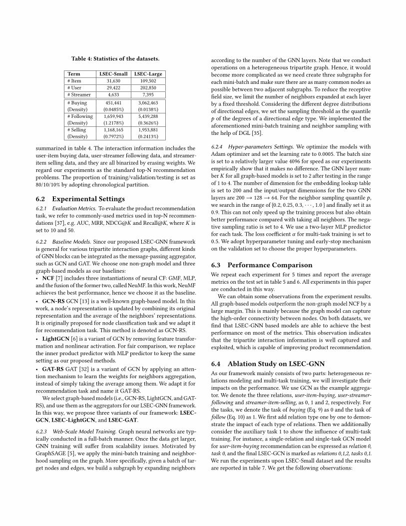
Table 4: Statistics of the datasets.
Term LSEC-Small LSEC-Large# Item 31,630 109,502
# User 29,422 202,850
# Streamer 4,633 7,395
# Buying 451,441 3,062,463
(Density) (0.0485%) (0.0138%)
# Following 1,659,943 5,439,288
(Density) (1.2178%) (0.3626%)
# Selling 1,168,165 1,953,881
(Density) (0.7972%) (0.2413%)
summarized in table 4. The interaction information includes the
user-item buying data, user-streamer following data, and streamer-
item selling data, and they are all binarized by erasing weights. We
regard our experiments as the standard top-N recommendation
problems. The proportion of training/validation/testing is set as
80/10/10% by adopting chronological partition.
6.2 Experimental Settings6.2.1 EvaluationMetrics. To evaluate the product recommendation
task, we refer to commonly-used metrics used in top-N recommen-
dations [37], e.g. AUC, MRR, NDCG@K and Recall@K, where 𝐾 is
set to 10 and 50.
6.2.2 Baseline Models. Since our proposed LSEC-GNN framework
is general for various tripartite interaction graphs, different kinds
of GNN blocks can be integrated as the message-passing aggregator,
such as GCN and GAT. We choose one non-graph model and three
graph-based models as our baselines:
• NCF [7] includes three instantiations of neural CF: GMF, MLP,
and the fusion of the former two, called NeuMF. In this work, NeuMF
achieves the best performance, hence we choose it as the baseline.
• GCN-RS GCN [13] is a well-known graph-based model. In this
work, a node’s representation is updated by combining its original
representation and the average of the neighbors’ representations.
It is originally proposed for node classification task and we adapt it
for recommendation task. This method is denoted as GCN-RS.
• LightGCN [6] is a variant of GCN by removing feature transfor-
mation and nonlinear activation. For fair comparison, we replace
the inner product predictor with MLP predictor to keep the same
setting as our proposed methods.
• GAT-RS GAT [32] is a variant of GCN by applying an atten-
tion mechanism to learn the weights for neighbors aggregation,
instead of simply taking the average among them. We adapt it for
recommendation task and name it GAT-RS.
We select graph-basedmodels (i.e., GCN-RS, LightGCN, andGAT-
RS), and use them as the aggregators for our LSEC-GNN framework.
In this way, we propose three variants of our framework: LSEC-GCN, LSEC-LightGCN, and LSEC-GAT.
6.2.3 Web-Scale Model Training. Graph neural networks are typ-
ically conducted in a full-batch manner. Once the data get larger,
GNN training will suffer from scalability issues. Motivated by
GraphSAGE [5], we apply the mini-batch training and neighbor-
hood sampling on the graph. More specifically, given a batch of tar-
get nodes and edges, we build a subgraph by expanding neighbors
according to the number of the GNN layers. Note that we conduct
operations on a heterogeneous tripartite graph. Hence, it would
become more complicated as we need create three subgraphs for
each mini-batch and make sure there are as many common nodes as
possible between two adjacent subgraphs. To reduce the receptive
field size, we limit the number of neighbors expanded at each layer
by a fixed threshold. Considering the different degree distributions
of directional edges, we set the sampling threshold as the quantile
𝑝 of the degrees of a directional edge type. We implemented the
aforementioned mini-batch training and neighbor sampling with
the help of DGL [35].
6.2.4 Hyper-parameters Settings. We optimize the models with
Adam optimizer and set the learning rate to 0.0005. The batch size
is set to a relatively larger value 4096 for speed as our experiments
empirically show that it makes no difference. The GNN layer num-
ber𝐾 for all graph-based models is set to 2 after testing in the range
of 1 to 4. The number of dimension for the embedding lookup table
is set to 200 and the input/output dimensions for the two GNN
layers are 200 → 128 → 64. For the neighbor sampling quantile 𝑝 ,
we search in the range of {0.2, 0.25, 0.3, · · · , 1.0 } and finally set it as0.9. This can not only speed up the training process but also obtain
better performance compared with taking all neighbors. The nega-
tive sampling ratio is set to 4. We use a two-layer MLP predictor
for each task. The loss coefficient 𝛼 for multi-task training is set to
0.5. We adopt hyperparameter tuning and early-stop mechanism
on the validation set to choose the proper hyperparameters.
6.3 Performance ComparisonWe repeat each experiment for 5 times and report the average
metrics on the test set in table 5 and 6. All experiments in this paper
are conducted in this way.
We can obtain some observations from the experiment results.
All graph-based models outperform the non-graph model NCF by a
large margin. This is mainly because the graph model can capture
the high-order connectivity between nodes. On both datasets, we
find that LSEC-GNN based models are able to achieve the best
performance on most of the metrics. This observation indicates
that the tripartite interaction information is well captured and
exploited, which is capable of improving product recommendation.
6.4 Ablation Study on LSEC-GNNAs our framework mainly consists of two parts: heterogeneous re-
lations modeling and multi-task training, we will investigate their
impacts on the performance. We use GCN as the example aggrega-
tor. We denote the three relations, user-item-buying, user-streamer-following and streamer-item-selling, as 0, 1 and 2, respectively. For
the tasks, we denote the task of buying (Eq. 9) as 0 and the task of
follow (Eq. 10) as 1. We first add relation type one by one to demon-
strate the impact of each type of relations. Then we additionally
consider the auxiliary task 1 to show the influence of multi-task
training. For instance, a single-relation and single-task GCN model
for user-item-buying recommendation can be expressed as relation 0,task 0, and the final LSEC-GCN is marked as relations 0,1,2, tasks 0,1.We run the experiments upon LSEC-Small dataset and the results
are reported in table 7. We get the following observations:
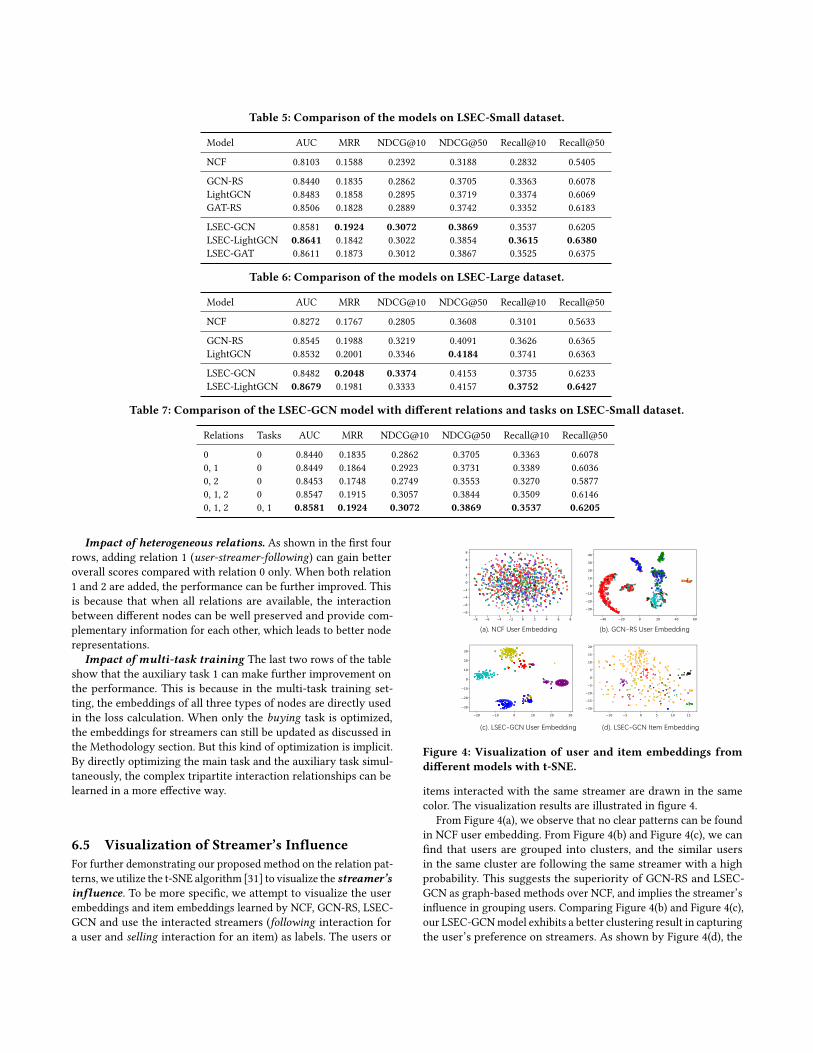
Table 5: Comparison of the models on LSEC-Small dataset.
Model AUC MRR NDCG@10 NDCG@50 Recall@10 Recall@50
NCF 0.8103 0.1588 0.2392 0.3188 0.2832 0.5405
GCN-RS 0.8440 0.1835 0.2862 0.3705 0.3363 0.6078
LightGCN 0.8483 0.1858 0.2895 0.3719 0.3374 0.6069
GAT-RS 0.8506 0.1828 0.2889 0.3742 0.3352 0.6183
LSEC-GCN 0.8581 0.1924 0.3072 0.3869 0.3537 0.6205
LSEC-LightGCN 0.8641 0.1842 0.3022 0.3854 0.3615 0.6380LSEC-GAT 0.8611 0.1873 0.3012 0.3867 0.3525 0.6375
Table 6: Comparison of the models on LSEC-Large dataset.
Model AUC MRR NDCG@10 NDCG@50 Recall@10 Recall@50
NCF 0.8272 0.1767 0.2805 0.3608 0.3101 0.5633
GCN-RS 0.8545 0.1988 0.3219 0.4091 0.3626 0.6365
LightGCN 0.8532 0.2001 0.3346 0.4184 0.3741 0.6363
LSEC-GCN 0.8482 0.2048 0.3374 0.4153 0.3735 0.6233
LSEC-LightGCN 0.8679 0.1981 0.3333 0.4157 0.3752 0.6427
Table 7: Comparison of the LSEC-GCN model with different relations and tasks on LSEC-Small dataset.
Relations Tasks AUC MRR NDCG@10 NDCG@50 Recall@10 Recall@50
0 0 0.8440 0.1835 0.2862 0.3705 0.3363 0.6078
0, 1 0 0.8449 0.1864 0.2923 0.3731 0.3389 0.6036
0, 2 0 0.8453 0.1748 0.2749 0.3553 0.3270 0.5877
0, 1, 2 0 0.8547 0.1915 0.3057 0.3844 0.3509 0.6146
0, 1, 2 0, 1 0.8581 0.1924 0.3072 0.3869 0.3537 0.6205
Impact of heterogeneous relations. As shown in the first four
rows, adding relation 1 (user-streamer-following) can gain better
overall scores compared with relation 0 only. When both relation
1 and 2 are added, the performance can be further improved. This
is because that when all relations are available, the interaction
between different nodes can be well preserved and provide com-
plementary information for each other, which leads to better node
representations.
Impact of multi-task training The last two rows of the table
show that the auxiliary task 1 can make further improvement on
the performance. This is because in the multi-task training set-
ting, the embeddings of all three types of nodes are directly used
in the loss calculation. When only the buying task is optimized,
the embeddings for streamers can still be updated as discussed in
the Methodology section. But this kind of optimization is implicit.
By directly optimizing the main task and the auxiliary task simul-
taneously, the complex tripartite interaction relationships can be
learned in a more effective way.
6.5 Visualization of Streamer’s InfluenceFor further demonstrating our proposed method on the relation pat-
terns, we utilize the t-SNE algorithm [31] to visualize the streamer’sinfluence. To be more specific, we attempt to visualize the user
embeddings and item embeddings learned by NCF, GCN-RS, LSEC-
GCN and use the interacted streamers (following interaction for
a user and selling interaction for an item) as labels. The users or
(c). LSEC-GCN User Embedding (d). LSEC-GCN Item Embedding
(b). GCN-RS User Embedding(a). NCF User Embedding
Figure 4: Visualization of user and item embeddings fromdifferent models with t-SNE.
items interacted with the same streamer are drawn in the same
color. The visualization results are illustrated in figure 4.
From Figure 4(a), we observe that no clear patterns can be found
in NCF user embedding. From Figure 4(b) and Figure 4(c), we can
find that users are grouped into clusters, and the similar users
in the same cluster are following the same streamer with a high
probability. This suggests the superiority of GCN-RS and LSEC-
GCN as graph-based methods over NCF, and implies the streamer’s
influence in grouping users. Comparing Figure 4(b) and Figure 4(c),
our LSEC-GCNmodel exhibits a better clustering result in capturing
the user’s preference on streamers. As shown by Figure 4(d), the

item embedding from our LSEC-GCN model also shows a similar
clustering result upon streamer’s influence on items, although not
as obvious as that from those of user embeddings. In short, the
visualization experiment not only shows the streamer’s influence
in connecting among users and items, but also indicates our LSEC-
GCN model’s ability to model the streamer’s influence.
7 CONCLUSIONIn this paper, we investigate a novel problem of how to leverage
the tripartite interaction information in live stream E-Commerce
to improve product recommendation. We conduct data analysis
on the collected real-world data. For the first time, we examine
three interaction patterns among streamers, users, and products,
and quantitatively study the streamer influence on users’ purchase
behavior. Based on the analysis results, we decompose the tripartite
interaction information into several bipartite graphs, and propose a
novel graph neural networks (LSEC-GNN) framework to aggregate
the node representations of bipartite graphs. We conduct exten-
sive experiments on two real-world live stream datasets, and the
results demonstrate that our method is effective to improve the
product recommendation performance. Moreover, we also present
the visualizations of streamer influence.
8 ACKNOWLEDGMENTSZhuoxuan Jiang is partially supported by Tencent Intelligent Media
Platform Project. Qi Liu and Sanshi Lei Yu acknowledge the support
of the USTC-JD joint lab. We thank the anonymous reviewers for
their insightful comments.
REFERENCES[1] Cheng Chen, Yuheng Hu, Yingda Lu, and Yili Hong. 2019. Everyone Can Be a Star:
Quantifying Grassroots Online Sellers’ Live Streaming Effects on Product Sales.
In Proceedings of the 52nd Hawaii International Conference on System Sciences.[2] Lei Chen, Le Wu, Richang Hong, Kun Zhang, and Meng Wang. 2020. Revisiting
Graph based Collaborative Filtering: A Linear Residual Graph Convolutional
Network Approach. In AAAI ’20.[3] Wenqi Fan, Yao Ma, Qing Li, Yuan He, Eric Zhao, Jiliang Tang, and Dawei Yin.
2019. Graph neural networks for social recommendation. InWWW ’19. 417–426.[4] Lauren Hallanan. 2020. Live Streaming Drives $6 Billion USD In Sales
During The 11.11 Global Shopping Festival. Retrieved February 7,
2021 from https://www.forbes.com/sites/laurenhallanan/2020/11/16/live-
streaming-drives-6-billion-usd-in-sales-during-the-1111-global-shopping-
festival/?sh=6671147c21e5
[5] William L Hamilton, Rex Ying, and Jure Leskovec. 2017. Inductive representation
learning on large graphs. arXiv preprint arXiv:1706.02216 (2017).[6] Xiangnan He, Kuan Deng, Xiang Wang, Yan Li, Yongdong Zhang, and Meng
Wang. 2020. LightGCN: Simplifying and Powering Graph Convolution Network
for Recommendation. In SIGIR ’20.[7] Xiangnan He, Lizi Liao, Hanwang Zhang, Liqiang Nie, Xia Hu, and Tat-Seng
Chua. 2017. Neural Collaborative Filtering. In WWW ’17. 173–182.[8] Balazs Hidasi, Alexandros Karatzoglou, Linas Baltrunas, and Domonkos Tikk.
[n.d.]. Session-based recommendations with recurrent neural networks.
[9] Zorah Hilvert-Bruce, James T. Neill, Max Sjöblom, and Juho Hamari. 2018. Social
motivations of live-streaming viewer engagement on Twitch. Computers inHuman Behavior 84 (2018), 58–67.
[10] Mingyao Hu and Sohail S Chaudhry. 2020. Enhancing consumer engagement in
e-commerce live streaming via relational bonds. Internet Research (2020).
[11] Yifan Hu, Yehuda Koren, and Chris Volinsky. [n.d.].
[12] Paul Jaccard. 2012. The distribution of the flora in the alpine zone. New Phytologist11, 2 (Feb. 2012), 37–50.
[13] Thomas N Kipf and MaxWelling. 2016. Semi-supervised classification with graph
convolutional networks. arXiv preprint arXiv:1609.02907 (2016).
[14] Yehuda Koren, Robert Bell, and Chris Volinsky. 2009. Matrix factorization tech-
niques for recommender systems. Computer 42 (2009), 30–37. Issue 8.[15] Joonseok Lee, Seungyeon Kim, Guy Lebanon, and Yoram Singer. [n.d.]. Local
low-rank matrix approximation.
[16] Chong Li, Kunyang Jia, Dan Shen, CJ Shi, and Hongxia Yang. 2019. Hierarchical
representation learning for bipartite graphs. In IJCAI ’19. 2873–2879.[17] Dongsheng Li, Chao Chen, Wei Liu, Tun Lu, Ning Gu, and Stephen Chu. [n.d.].
Mixture-Rank Matrix Approximation for Collaborative Filtering.
[18] Dawen Liang, Rahul G Krishnan, Matthew D Hoffman, and Tony Jebara. [n.d.].
Variational autoencoders for collaborative filtering.
[19] Zhicong Lu, Haijun Xia, Seongkook Heo, and Daniel Wigdor. 2018. You Watch,
You Give, and You Engage: A Study of Live Streaming Practices in China. In CHI’18.
[20] Steffen Rendle, Christoph Freudenthaler, Zeno Gantner, and Lars Schmidt-Thieme.
[n.d.]. BPR: Bayesian Personalized Ranking from Implicit Feedback.
[21] Ruslan Salakhutdinov and Andriy Mnih. [n.d.]. Bayesian Probabilistic Matrix
Factorization Using Markov Chain Monte Carlo.
[22] Katrin Scheibe, Kaja J. Fietkiewicz, and Wolfgang G. Stock. 2016. Information
Behavior on Social Live Streaming Services. Journal of Information Science Theoryand Practice 4, 2 (2016), 6–20.
[23] Suvash Sedhain, Aditya Krishna Menon, Scott Sanner, and Lexing Xie. [n.d.].
AutoRec: Autoencoders Meet Collaborative Filtering.
[24] Xiao Sha, Zhu Sun, and Jie Zhang. 2019. Attentive Knowledge Graph Embedding
for Personalized Recommendation. In arXiv preprint arXiv:1910.08288.[25] Chih-Ya Shen, CP Kankeu Fotsing, De-Nian Yang, Yi-Shin Chen, andWang-Chien
Lee. [n.d.]. On organizing online soirees with live multi-streaming.
[26] Weiping Song, Zhiping Xiao, Yifan Wang, Laurent Charlin, Ming Zhang, and Jian
Tang. [n.d.]. Session-based social recommendation via dynamic graph attention
networks.
[27] Yuan Sun, Xiang Shao, Xiaotong Li, Yue Guo, and Kun Nie. 2019. How live
streaming influences purchase intentions in social commerce: An IT affordance
perspective. Electronic Commerce Research and Applications 37 (2019), 1–12.[28] Qiaoyu Tan, Ninghao Liu, Xing Zhao, Hongxia Yang, Jingren Zhou, and Xia Hu.
2020. Learning to Hash with Graph Neural Networks for Recommender Systems.
In WWW ’20. 1988–1998.[29] Gerald Tesauro and Gregory R. Galperin. [n.d.]. On-line policy improvement
using Monte-Carlo search.
[30] Rianne van den Berg, ThomasNKipf, andMaxWelling. 2018. Graph ConvolutionalMatrix Completion.
[31] Laurens Van der Maaten and Geoffrey Hinton. 2008. Visualizing data using t-SNE.
Journal of machine learning research 9, 11 (2008).
[32] Petar Veličković, Guillem Cucurull, Arantxa Casanova, Adriana Romero, Pietro
Lio, and Yoshua Bengio. 2017. Graph attention networks. arXiv preprintarXiv:1710.10903 (2017).
[33] Hongwei Wang, Fuzheng Zhang, Mengdi Zhang, Jure Leskovec, Miao Zhao,
Wenjie Li, and ZhongyuanWang. 2019. Knowledge-aware graph neural networks
with label smoothness regularization for recommender systems. In KDD ’19.968–977.
[34] Hongwei Wang, Miao Zhao, Xing Xie, Wenjie Li, and Minyi Guo. 2019. Knowl-
edge Graph Convolutional Networks for Recommender Systems. InWWW ’19.1210–1221.
[35] Minjie Wang, Da Zheng, Zihao Ye, Quan Gan, Mufei Li, Xiang Song, Jinjing Zhou,
Chao Ma, Lingfan Yu, Yu Gai, Tianjun Xiao, Tong He, George Karypis, Jinyang
Li, and Zheng Zhang. 2019. Deep Graph Library: A Graph-Centric, Highly-
Performant Package for Graph Neural Networks. arXiv preprint arXiv:1909.01315(2019).
[36] XiangWang, Xiangnan He, Yixin Cao, Meng Liu, and Tat-Seng Chua. 2019. KGAT:
Knowledge graph attention network for recommendation. In KDD ’19. 950–958.[37] Xiang Wang, Xiangnan He, Meng Wang, Fuli Feng, and Tat-Seng Chua. 2019.
Neural graph collaborative filtering. In SIGIR ’19. 165–174.[38] Xiao Wang, Ruijia Wang, Chuan Shi, Guojie Song, and Qingyong Li. 2020. Multi-
Component Graph Convolutional Collaborative Filtering. In AAAI ’20.[39] Chao-Yuan Wu, Amr Ahmed, Alex Beutel, Alexander J Smola, and How Jing.
[n.d.]. Recurrent recommender networks.
[40] Le Wu, Peijie Sun, Yanjie Fu, Richang Hong, Xiting Wang, and Meng Wang.
2019. A neural influence diffusion model for social recommendation. In SIGIR’19. 235–244.
[41] Qitian Wu, Hengrui Zhang, Xiaofeng Gao, Peng He, PaulWeng, Han Gao, and
Guihai Chen. 2019. Dual graph attention networks for deep latent representation
of multifaceted social effects in recommender systems. InWWW ’19. 2091–2102.[42] J. Yu, H. Yin, J. Li, M. Gao, Z. Huang, and L. Cui. 2020. Enhance Social Recom-
mendation with Adversarial Graph Convolutional Networks. IEEE Transactionson Knowledge and Data Engineering 01 (oct 2020), 1–1. https://doi.org/10.1109/
TKDE.2020.3033673
[43] Jiani Zhang, Xingjian Shi, Shenglin Zhao, and Irwin King. 2019. STAR-GCN:
stacked and reconstructed graph convolutional networks for recommender sys-
tems. In IJCAI ’19. 4264–4270.[44] Muhan Zhang and Yixin Chen. 2020. Inductive matrix completion based on graph
neural networks. In ICLR ’20.