Embed Size (px)
Citation preview
LEVERAGING PRODUCTION OUTPUT THROUGH
INDEX-PARALLEL TESTING
TECHNOLOGY
A Project Presented to the Faculty
of
California State University, Stanislaus
In Partial Fulfillment
of the Requirements for the Degree
of Master of Business Administration
By
Hector Valdez
August 2017
Signed Certification of Approval page
is on file with the University Library
CERTIFICATION OF APPROVAL
LEVERAGING PRODUCTION OUTPUT THROUGH
INDEX-PARALLEL TESTING
TECHNOLOGY
By
Hector Valdez
Dr. Jingyun Li
Faculty Advisor, Professor of Management
Operations and Marketing
Dr. Sophie Zong
Project Coordinator, Professor of Finance
Ms. Katrina Kidd
Director of MBA Program
Dr. Tomas Gomez-Arias
Dean of College of Business Administration
Date
Date
Date
Date

© 2017
Hector Valdez
ALL RIGHTS RESERVED

iv
ACKNOWLEDGEMENTS
This project is a culmination of my MBA study. It would not have been
possible if not for the people behind it. Thus, I owe a debt of gratitude to them who
have helped and inspired me to write and finish this project.
My profound appreciation of my wife, Sally, and my children, Christian and
Christine, for the love and understanding they provided while I was writing this
project. A big hug for Christian, who meticulously reviewed my document through
the late hours of the night.
I am also gratefully indebted to my project adviser, Professor Jingyun Li, who
patiently reviewed and offered valuable comments and ideas for the improvement of
this project. A heartfelt thank you to all my professors, Dir. Katrina Kidd, Prof. Ann
Edwards, Prof. Steven Filling, Prof. Tahi Gnepa, Prof. Andrew Hinrichs, Prof. Jarrett
Kotrozo, Prof. Jennifer Leonard, Prof. Esteban Montes, Prof. Feng Zhou, Prof.
Xiaozhou Zhu, Prof. Sijing Zong, and to the other faculty members who throughout
the course of the MBA program have enlightened me to the theories and principles of
Management which I applied successfully in this project.
To God be the glory.
v
TABLE OF CONTENTS
PAGE
Acknowledgements ................................................................................................. iv
List of Tables .......................................................................................................... vii
List of Figures ......................................................................................................... ix
Abstract ................................................................................................................... x
CHAPTER
I. Introduction to the Study ...................................................................... 1
Background ............................................................................... 1
Statement of the Problem .......................................................... 4
Purpose of the Study ................................................................. 5
Significance of the Study .......................................................... 5
Research Questions ................................................................... 6
Delimitations and Limitations of the Study .............................. 6
II. Methodology ......................................................................................... 8
Definition of Terms................................................................... 8
Specific Procedures ................................................................... 10
Instrumentation ......................................................................... 10
Test System Configuration ....................................................... 11
Pilot Study ................................................................................. 14
Data Collection ......................................................................... 15
Data Analysis Procedures ......................................................... 17
III. Results ................................................................................................... 30
Plan of the Study ....................................................................... 30
Descriptive Statistics ................................................................. 30
Research Questions ................................................................... 39
Research Question One ....................................................... 39
Research Question Two ...................................................... 41
Research Question Three .................................................... 43
Additional Analyses .................................................................. 48
IV. Discussion, Recommendations, and Conclusions ................................ 53
vi
Discussion of the Findings ........................................................ 53
Recommendations for Further Research ................................... 55
Conclusions ............................................................................... 56
References ............................................................................................................... 58
Appendices
A. ASL 1000 (ATE) Specification .................................................................. 61
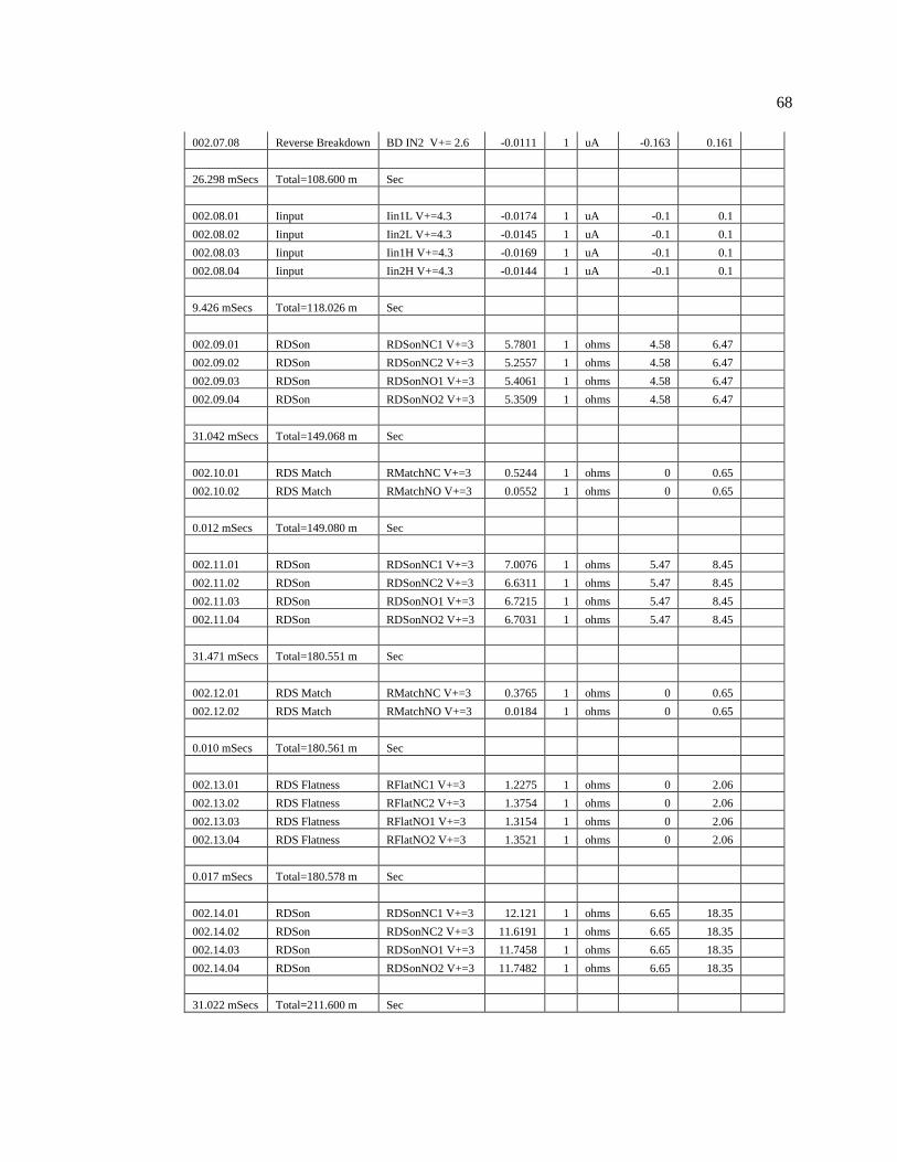
B. Device Test Datalog .................................................................................... 65
1. Quad-Site MOSFET Datalog ................................................................ 65
2. Index-Parallel MOSFET Datalog ......................................................... 66
3. Single-Site IC Datalog .......................................................................... 67
4. Dual-Site IC Datalog............................................................................. 71
C. Device Datasheets ....................................................................................... 75
1. FDD8896 / FDU8896 Datasheet ........................................................... 75
2. MAX4993 Datasheet ............................................................................ 77
D. System Configurations ................................................................................ 80
1. Quad-Site Full Parallel System Configuration ..................................... 80
2. Index-Parallel System Configuration ................................................... 81
E. SRM XD 326 Rotary Handler Specification .............................................. 82
vii
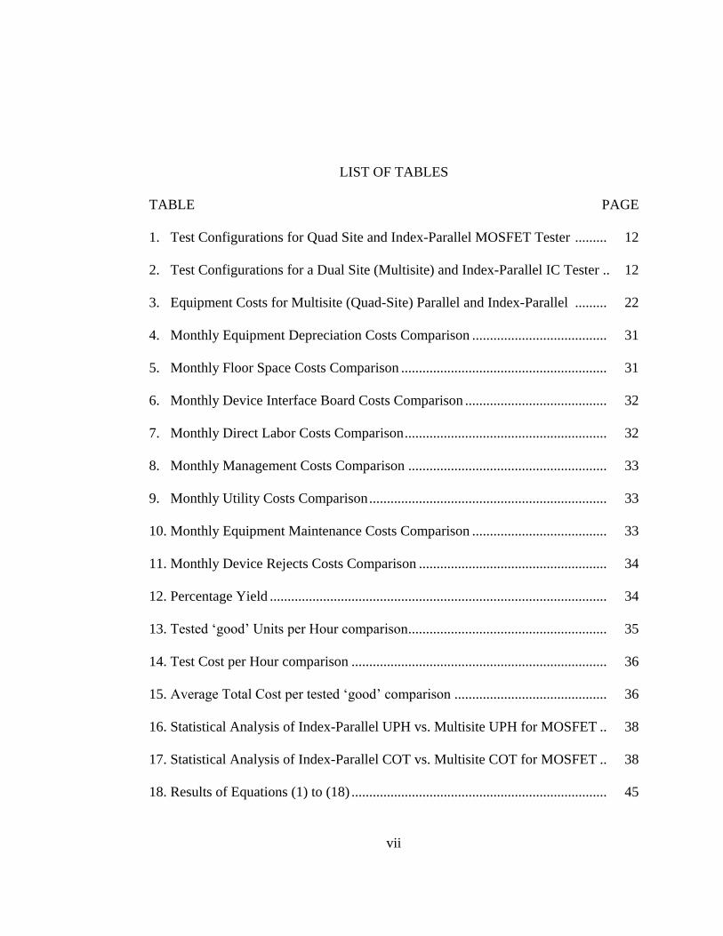
LIST OF TABLES
TABLE PAGE
1. Test Configurations for Quad Site and Index-Parallel MOSFET Tester ......... 12
2. Test Configurations for a Dual Site (Multisite) and Index-Parallel IC Tester .. 12
3. Equipment Costs for Multisite (Quad-Site) Parallel and Index-Parallel ......... 22
4. Monthly Equipment Depreciation Costs Comparison ...................................... 31
5. Monthly Floor Space Costs Comparison .......................................................... 31
6. Monthly Device Interface Board Costs Comparison ........................................ 32
7. Monthly Direct Labor Costs Comparison ......................................................... 32
8. Monthly Management Costs Comparison ........................................................ 33
9. Monthly Utility Costs Comparison ................................................................... 33
10. Monthly Equipment Maintenance Costs Comparison ...................................... 33
11. Monthly Device Rejects Costs Comparison ..................................................... 34
12. Percentage Yield ............................................................................................... 34
13. Tested ‘good’ Units per Hour comparison........................................................ 35
14. Test Cost per Hour comparison ........................................................................ 36
15. Average Total Cost per tested ‘good’ comparison ........................................... 36
16. Statistical Analysis of Index-Parallel UPH vs. Multisite UPH for MOSFET .. 38
17. Statistical Analysis of Index-Parallel COT vs. Multisite COT for MOSFET .. 38
18. Results of Equations (1) to (18) ........................................................................ 45
viii
19. Statistical Analysis of Index-Parallel UPH and Multisite UPH for IC ............. 46
20. Statistical Analysis of Index-Parallel COT and Multisite COT for IC ............. 47
21. Cost Savings Analysis....................................................................................... 51
ix
LIST OF FIGURES
FIGURE PAGE
1. IC Fabrication Process ...................................................................................... 2
2. Quad Site Full Parallel Test Time Map of MOSFET Transistor ..................... 18
3. Index-Parallel Test Time Map of MOSFET Transistor ................................... 19
4. Distribution of Test Time for FT and QA using Quad-Site Parallel Testing ... 21
5. Test time distribution of Index-Parallel FT and QA ........................................ 21
6. Dual-Site Full Parallel Test Time Map of IC Device ...................................... 28
7. Index-Parallel test time map of IC device ......................................................... 29
8. Good yield distribution from 95% to 100% ..................................................... 37
9. Multisite Parallel UPH Bell Curve Distribution .............................................. 39
10. Index-Parallel UPH Bell Curve Distribution ................................................... 40
11. Comparative UPH Distributions of both Multisite and Index-Parallel ........... 41
12. Multisite Parallel COT Histogram ................................................................... 42
13. Index-Parallel COT Histogram ........................................................................ 42
14. Histograms of Multisite and Index-Parallel ..................................................... 42
15. Comparative UPH Histograms of Multisite and Index-Parallel for IC............. 46
16. Overlaid Histograms of Multisite and Index-Parallel COTs ............................ 48
17. UPH Delta Histogram and Statistics for Transistor .......................................... 49
18. UPH Delta Histogram and Statistics for IC ...................................................... 50
x
ABSTRACT
Index-Parallel testing technology is a relatively new concept in semiconductor testing
that can be used to leverage production output and reduces the cost of testing. This
study explains the methodologies of single site and multisite testing and introduces
the concept of Index-Parallel testing. With the implementation of Index-Parallel
testing high production throughput as a result of reduced test time and required
resources can be achieved, thus increasing production output and lowering the Cost of
Test (COT) with a significant overall savings over time. The reduction in total test
time significantly improved the throughput of the test system and lowered the
Average Test Cost. The implementation of Index-Parallel produced a 24% increase
in throughput for transistor testing and a 20% increase for integrated circuit (IC)
testing compared to Multisite. As a result, the Costs of Test were reduced by an
average of 0.13¢ for transistor testing and an average of 0.31¢ for IC testing. The
increase in throughput coupled with the reduction of Cost of Test verified the
advantages of Index-Parallel technique for transistor device testing and successfully
applied the same principle to the relatively more complex IC device. The findings
not only confirmed its effectiveness in production, but also confirmed the economic
advantages of using Index-Parallel technology in semiconductor manufacturing.
1
CHAPTER I
INTRODUCTION TO THE STUDY
Background
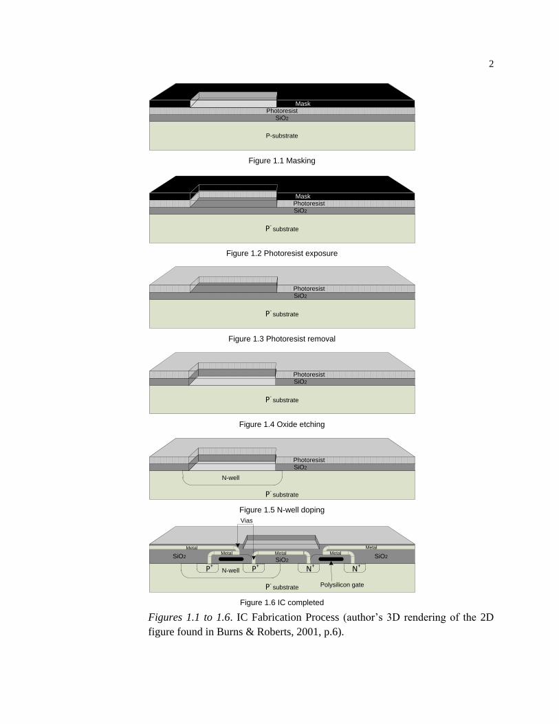
Semiconductor devices, such as discrete transistors and integrated circuits
(IC), are manufactured using a series of photolithographic printing, etching, and
doping processes. Fabrication starts with a lightly doped P-type silicon wafer, which
is created by adding precise amounts of donor impurity atoms such as boron into a
molten intrinsic silicon material changing it into a P-type extrinsic semiconductor. P-
type semiconductors have more positive charge hole concentration than electron
concentration. A layer of silicon dioxide (SiO2) is added to the surface of the P-type
silicon wafer (Figure 1.1). Then, a negative photoresist is set on top of the silicon
dioxide. Next, using a photographic mask, ultraviolet light is projected onto the
photoresist. Areas where the mask allows the ultraviolet light to reach become
insoluble (Figure 1.2). An organic solvent is then applied to dissolve the areas of the
photoresist that have not been exposed to the ultraviolet light (Figure 1.3). The
exposed areas of oxide are removed using an etching process after baking the
remaining photoresist (Figure 1.4). Using either ion implantation or diffusion
technique, the exposed areas of silicon are then doped to form an N-well (Figure 1.5).
Additional processing steps of printing, masking, etching, implanting, and chemical
vapor deposition are repeated to complete a semiconductor circuit (Figure 1.6) (Burns
& Roberts, 2001, p.5).
2
P-substrate
SiO2
Photoresist Mask
P- substrate
SiO2
Photoresist Mask
P- substrate
SiO2
Photoresist
P- substrate
P- substrate
SiO2
Photoresist
P- substrate
SiO2
Photoresist
N-well
N-wellP+ P+
MetalMetal Metal
Metal
Metal
N+ N+
Vias
SiO2SiO2SiO2
Polysilicon gate
Figure 1.1 Masking
Figure 1.2 Photoresist exposure
Figure 1.3 Photoresist removal
Figure 1.4 Oxide etching
Figure 1.5 N-well doping
Figure 1.6 IC completed
Figures 1.1 to 1.6. IC Fabrication Process (author’s 3D rendering of the 2D
figure found in Burns & Roberts, 2001, p.6).
3
The semiconductor photographic printing process is not immune to
imperfections. These imperfections can cause catastrophic functional failures of any
semiconductor device, or generate slight variations in performance from device to
device. Semiconductor devices are extremely sensitive to defects or even small
variations in the photographic printing and doping processes. Manufacturing defects
that can cause problems in semiconductor devices are not easy to detect even with the
use of a powerful scanning electron microscope (SEM). Semiconductor doping
process errors may or may not cause an observable physical defect or one that can be
caught by the naked eye. However, doping errors can cause problems with the
functionality that leads to the device’s performance failures (Burns & Roberts, 2001,
p.5). These kinds of defects are often easier to detect using semiconductor test
equipment. Thus, final testing and quality testing after fabrication are necessary and
required with the use of these testers.
Production testing of semiconductor devices, like discrete and integrated
circuits (IC), is an essential part in manufacturing of electronic devices. It prevents
the defective devices from getting through to the finishing process and customers,
thereby eliminating quality issues and customer returns. The goal is to achieve zero
defect from going through the last stage of manufacturing and this can be attained at
final testing (FT) and quality assurance (QA) testing. It is a costly but important
process in the final step of manufacturing semiconductor devices, guaranteeing the
reliability and functionality of the finish product. This step ensures the device meets
4
the specifications in its datasheet, an important requirement in the design of consumer
products like computers, smartphones, and other electronic appliances.
Final testing of semiconductor devices has always been performed using
either single-site or multisite parallel testing. High production throughput can be
achieved using the latter method, and has become the industry standard in production
testing of semiconductor devices. However, final testing including the intensive time
spent on development is expensive, requiring significant monetary investment in
manpower, material, and test equipment, and can cost hundreds of thousands of
dollars. Thus, a new method is needed to address the problem of throughput and the
cost of test.
A testing methodology, though little known to the semiconductor industry, is
called Index-Parallel Testing. It is a method that can significantly increase the
throughput of a production test machine, and lower the Cost-of-Test (COT) as well as
the costs of the required capital equipment. Immediate savings of hundreds of
thousands of dollars on the cost of production testing and on capital equipment
spending can be realized. Savings in the millions can be achieved throughout its life
cycle.
Statement of the Problem
Testing of semiconductor devices is an expensive, yet essential step in
semiconductor manufacturing. It guarantees that the finished product adheres to
quality, reliability, and accuracy standards. Depending on the type and complexity of
the semiconductor device to test, the cost-of-test can vary widely from device to
5
device. This study will focus on simple semiconductor transistor devices and more
complex analog semiconductor integrated circuit (IC) devices. The goal is to find an
efficient and cost-effective solution for both types of devices.
Purpose of the Study
The main purpose of this study is to validate the effectiveness of Index-
Parallel testing on semiconductor transistors regarding improving production
throughput and reducing the Cost-of-Test (COT). Moreover, this study explores
applying the same principle on a more complex analog semiconductor device and
achieving similar increase in throughput.
Significance of the Study
This study is important to the successful implementation of Index-Parallel
technology as it provides an alternative solution to costly semiconductor testing.
Potential impact of this study may span to the development of implementation
procedures in test methodology for the effective use of Index-Parallel technology,
which improves throughput and lowers cost.
Attempts have been made to expand the current Multisite technology by
increasing the number of sites, only to find that it proportionally increases the cost
which in the end, invalidates its cost effectiveness. Many manufacturers of Multisite
equipment have tried to further improve what is left of its advantage. Semiconductor
manufacturers, on the other hand, continuously improve their product’s output by
yield analysis engineering. Many are overlooking the fact that the cost of testing also
plays a pivotal role in the determination of the price of the product. Thus, this study is
6
important in finding an alternative solution to semiconductor device testing. The
successful implementation of Index-Parallel technology in semiconductor
manufacturing will contribute in the advancement, cost reduction, and speed of
semiconductor testing.
Research Questions
The following research questions were presented to address the economy of
semiconductor manufacturing, specifically at the final test (FT) and quality control
(QC) testing stages of the finished product.
1. Will the use of Index-Parallel test technology address the inefficiency of
the current Multisite testing technology and improve the throughput of production
testing?
2. Will the use of Index-Parallel test technology become a viable solution in
reducing the cost-of-testing (COT) in semiconductor manufacturing?
3. Can the same principle be applied from a simple semiconductor transistor
device to a relatively more complex semiconductor integrated circuit (IC) device?
Delimitations and Limitations of the Study
The delimitations of the study include the various levels of the complexity of
devices from a three-terminal transistor device to a multipin integrated circuit (IC)
that were used in the study. The study was thus delimited to a simple Metal Oxide
Semiconductor Field Effect Transistor (MOSFET) transistor and a more complex
analog switch IC, but not to the most complex levels such as the microprocessor IC.
7
The level of complexity requires a significantly proportional amount of investment of
both time and resources.
Differences in the capabilities of various semiconductor test systems or test
machines also delimits the scope of this study. Like having variations in the
complexity of semiconductor devices mentioned above, variations also exist in the
applications of different test systems.
Due to the high-volume demand in IC device testing in production, the IC
devices used as test vehicles in this study were already tested during the early part of
the year. Thus, the IC devices were already transferred to Marketing and no longer
available in Production. However, since the data have already been taken, they were
available for use in the study.
8
CHAPTER II
METHODOLOGY
Definition of Terms
The following are definitions of the technical terms used in this study.
Automated Test Equipment (ATE). An automated test equipment or ATE is a
computer-controlled electronic system made up of instrumentations that can force and
measure different test parameters of electronic devices for functionality and
performance. ATE performs parametric and stress testing with minimal human
interaction. An ATE is comprised of a main computer, hardware controller, forcing
and measuring instruments, device interface, and software that collects and analyzes
the test results.
Single-site testing. Single site testing is a test methodology wherein an Automated
Test Equipment (ATE) performs a complete test of device’s parameters one site at a
time. The ATE system configuration includes a single-site device interface and an
automated single-site handler for continuous testing.
Multisite testing. Multisite testing is an improved test methodology over single-site
testing wherein an ATE performs a complete test of all the parameters of a number of
the same devices simultaneously in parallel. The configuration can be dual-site (two
devices tested in parallel), quad-site (four devices tested in parallel), or N-site (N
number of devices tested in parallel). The ATE system configuration may use a dual-
9
site, quad-site, or an N-site device interface connected to an automated multisite
parallel handler that corresponds to the number of sites to test for continuous testing.
Index-Parallel testing. Index-Parallel testing differs in implementation compared to
the single-site or multisite. Index-Parallel testing is a test methodology that uses
device indexing wherein an N number of devices are sequentially transferred,
indexed, and tested partially from one station to the next. The indexed partial test
results are then stitched together to form one complete record or datalog of each
device tested. The ATE system configuration will comprise of N number of device
interface installed to an automated rotary handler for N number of stations for
continuous testing.
Cost-of-Test (COT). Cost-of-Test (COT) is the amount or cost associated in testing
one device. A number of factors are considered in determining this value; i.e. test
equipment depreciation costs, direct labor costs, overhead costs, and cost of reject
parts. COT is also dependent on the test coverage and the complexity of the device to
test which defines the amount of time a device is tested.
Index time. For rotary handlers, it is the amount of time it takes to shuttle a Device
Under Test (DUT) from one site to the next site for testing. For multisite handlers, it
is the time it takes to transfer a DUT from queue to the test site for testing.
Units per Hour (UPH). The unit of measure that defines the number of devices tested
in a span of 1 hour. Extensively used with lean manufacturing, it is a unit of measure
10
that is used in comparing the speed of test systems or a measure of machine
downtime.
Specific Procedures
Research was first conducted to assess the feasibility of the project. Decisions
needed to be made on what semiconductor devices to use; for example, should the
researchers design the board electronics that would hold the device or use an existing
production equipment setup. Existing program and production tester equipped with
instrumentations necessary to perform the test were used to collect the preliminary
datalog of test measurements for the analysis. The instrumentations are measuring,
forcing, and digitizing analog or digital electronic circuits and resources that are
plugged into the ATE tester. System clock instrumentation were also needed. If
available, a rotary handler would be used, which attaches to the tester for automatic
device handling of hundreds of test devices. Calibration equipment might be needed.
Statistical software was then used to analyze the collected datalog.
Instrumentation
A major part of this study used a test system which comprises a set of
instrumentations, peripheral hardware, and software to measure the readings which
are reported in the form of a datalog. These datalogs are essential in validating the
outcome of our study. The following lists all the instrumentations used and explains
their purpose in the study.
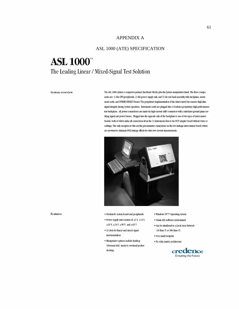
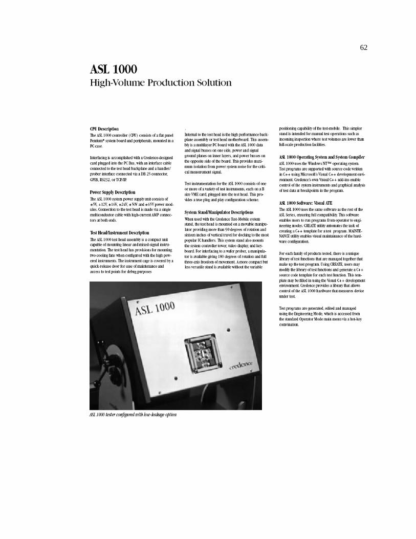
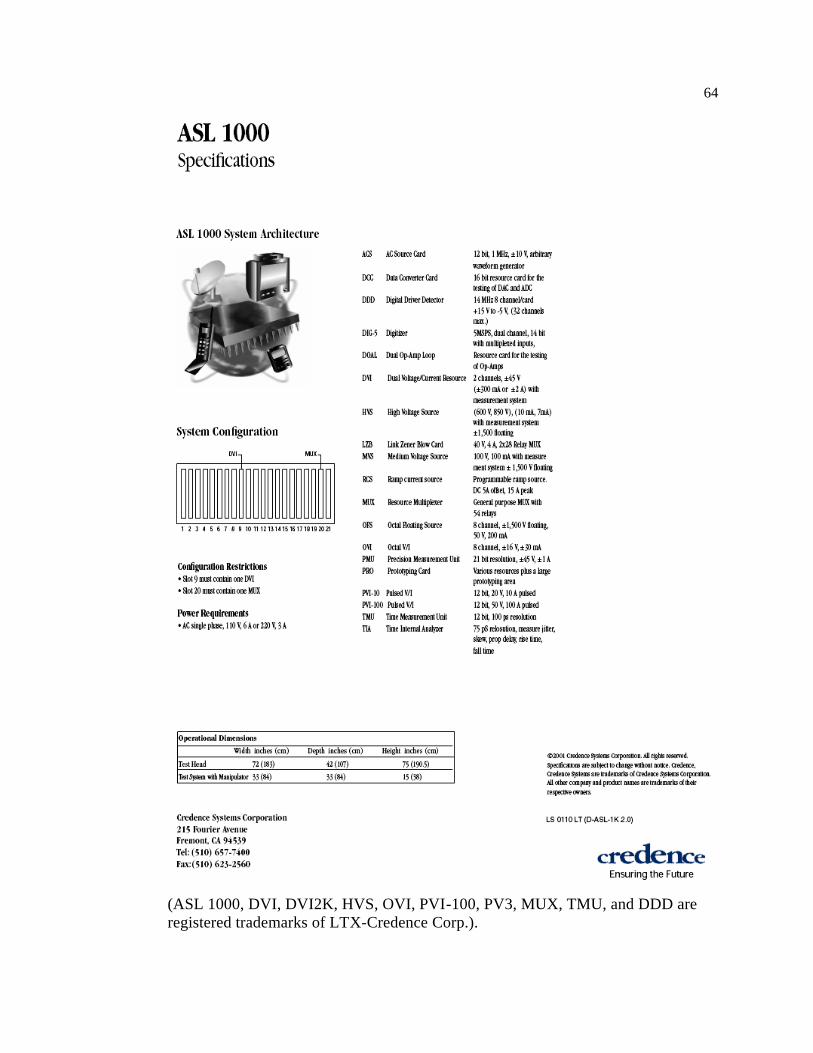
The ASL 1000 stands for Automated Series Linear 1000 tester. It is a linear
mixed signal tester designed to test electronic components from transistors to
11
integrated circuits (ICs) at high speed. It is comprised of the three primary hardware
blocks: 1) the computer (CPU and peripherals) that controls the entire system, 2) the
power supply that provides power to the system, and 3) the test head assembly with
21 slots backplane where the forcing and measuring linear and mixed-signal
instruments are plugged in. It uses MS Visual C++ to create the test program for the
study and proprietary software to control the system. These software components
enable users to run the system in production environment settings.
For production testing, a rotary handler such as the SRM XD206 is required
for volume testing. The SRM XD206 is an automated rotary handling machine that
can be connected to a tester such as ASL 1000, to assist in sorting and setting
transistor or IC devices for testing. It can be set in a variety of configurations with
Vision Inspection and Laser Marking stages that allows it to perform complete Final
Test (FT) and Quality Control (QC) testing in a production setting. It is capable of
handling up to 40,000 Units Per Hour (UPH) depending on the speed of the tester.
Rotary handlers can also be configured to run in both Multisite parallel or Index-
Parallel testing with Index-Parallel gaining more advantage with a higher
throughput (UPH).
Test System Configuration
A test system requires specific configuration for specific devices to test. The
test configuration comprises a combination of different instrumentations plugged into
the ASL 1000 backplane and performs the forcing and measuring of the test
parameters of the devices to test, more commonly referred to in test engineering as
12
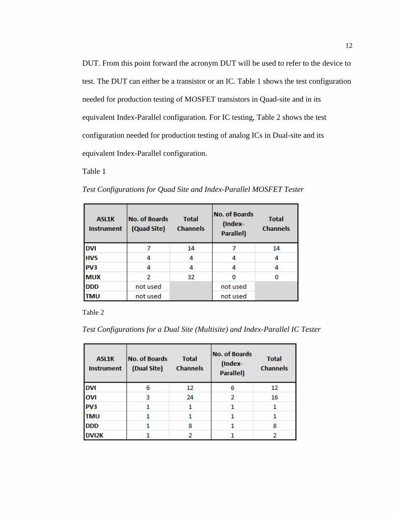
DUT. From this point forward the acronym DUT will be used to refer to the device to
test. The DUT can either be a transistor or an IC. Table 1 shows the test configuration
needed for production testing of MOSFET transistors in Quad-site and in its
equivalent Index-Parallel configuration. For IC testing, Table 2 shows the test
configuration needed for production testing of analog ICs in Dual-site and its
equivalent Index-Parallel configuration.
Table 1
Test Configurations for Quad Site and Index-Parallel MOSFET Tester
Table 2
Test Configurations for a Dual Site (Multisite) and Index-Parallel IC Tester
13
The instrumentation used are briefly defined as follows:
DVI or DVI2K. Stands for Dual Voltage and Current. It is a two channel
independent four-quadrant force and measure instrument. Capable of forcing
voltage to ±45V and current to ±2A while measuring voltage up to 100V and
current up to 2A. This instrument is used to measure the DC parameters of DUT.
HVS. Stands for High Voltage floating Source. It is a sourcing and
measuring instrument that is capable of delivering a maximum high voltage of
600V at 10uA of low current and can be stacked up to ±1,500V. It has a maximum
voltage measuring range of 1,000V and a low current measuring range of 10mA.
This instrument is used for sourcing and measuring high voltage MOSFETs or IC
devices.
OVI. Octal Voltage and Current. The OVI is an eight-channel independent
four full quadrant force and measure instrument capable of forcing a low voltage up
to ±20V and low current up to 30mA while measuring the same maximum amount
of voltage and current at an accuracy of ±0.1% of range. This instrument can
perform up to eight simultaneous force and measure on a test device.
PVI-100 or PV3 is a Pulsed Voltage and Current instrument that can force a
100A pulsed current at 20V or 1A at 50V. Simultaneously, it can measure voltage
while forcing current and vice versa. This is a floating instrument for generating
high current pulses for testing high-current devices.
MUX is short for Multiplexer. The MUX is comprised internally of an array
of 64 programmable electromechanical relays or switches. The relays can withstand
14
a maximum operating voltage of 500V and maximum current of 1.5A. Its 64
channel resource multiplexer can be programmed to interconnect with the test
device, with other instruments, or a combination of both.
TMU or Timing Measurement Unit is designed to measure time between
intervals. Its regular inputs can measure up to 10V signals while its four high-
impedance inputs have a maximum range of ±1000V. It is used in testing the timing
parameters, such as turn on or turn off times of both analog and digital test devices.
DDD is the acronym for Digital Driver and Detector. The DDD is a general
purpose eight channel high speed digital input and output (I/O) instrument designed
for stimulation and readback of digital and mixed-signal test devices. Its built-in
memory can hold 32K (thousands) of patterns of highs and lows and its expandable
to 128K. Its high speed driver can generate an output up to 15V at a speed of
28MHz.
More information about ASL 1000 test system can be found at Appendix A.
(ASL 1000, DVI, DVI2K, HVS, OVI, PVI-100, PV3, MUX, TMU, and DDD are
registered trademarks of LTX-Credence Corp.)
Pilot Study
A pilot study was conducted to determine the project’s feasibility prior to
proceeding with the Index-Parallel study. The pilot study was conducted on Qua-
site (Multisite) configuration for both the MOSFET transistor and the analog IC. An
existing Quad Site MOSFET test program, ATE hardware, and Device Interface
Board (DIB) were used to collect the readings from four MOSFET DUTs run in
15
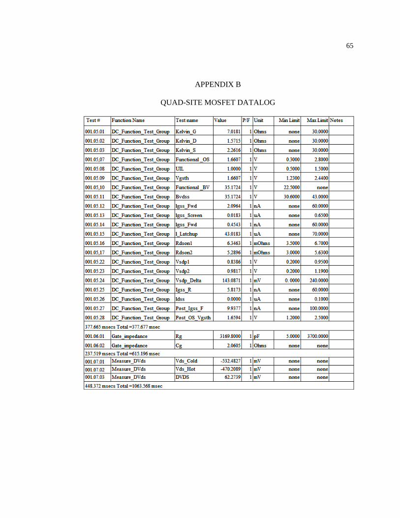
multisite parallel. The resulting datalog ‘Quad Site MOSFET Datalog’ in Appendix
B defines the test parameters and the test time baselines for the MOSFET transistor
that were used to compare with the Index-Parallel results. The test parameters listed
in the datalog were used to develop the Index-Parallel equivalent test program.
Similarly, an existing Dual Site IC test program, ATE hardware, and DIB
board were used to collect the readings from two IC DUTs run in multisite parallel.
The resulting datalog ‘Dual Site IC Datalog’ in Appendix B defines the test
parameters and test time as baselines for the IC. These data were used to develop
and compare the results of the Index-Parallel Solution.
Data Collection
This study utilized the quantitative method of data collection and analysis.
With the use of an ATE test system setup with the configuration shown in Table 1,
device’s test program written for MOSFET transistors, and DIB board data can be
collected in the form of readings of each of the parameters and reported as datalog.
Each parameter to be measured is listed in the DUT’s datasheet or specification.
The “FDD8896/FDU8896 Datasheet” shown in Appendix C is representative of the
different MOSFET part numbers. It shows the various tests used to measure
voltage, current, resistance, etc. The test conditions or stimulus for each test
parameters were injected by the ATE test system and the DUT’s output response
was measured by the ATE as well. Each of these measurements were then compared
with the DUT’s high and low limits provided in the datasheet. ‘Quad Site MOSFET
Datalog’ in Appendix B shows the measurement results in the form of a datalog.
16
After determining the test parameters and the baseline values needed from
the resulting Quad-Site MOSFET datalog, specifically the test measurement results
and test time breakdowns, it was then possible to formulate an Index-Parallel
equivalent solution that would answer the research questions. From this information
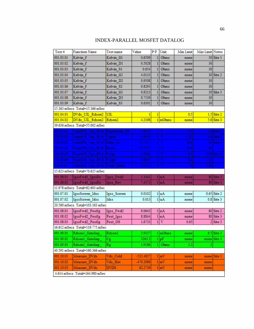
an Index-Parallel program algorithm was developed. The ATE test system was
configured to run the Index-Parallel program. The resulting datalog is shown in
Appendix B, ‘Index-Parallel MOSFET Datalog.’ Multiple test runs were then
performed on both Quad-Site and Index-Parallel configurations with the aid of an
automated rotary handler for easier and faster collection of datalog to be used for
statistical and comparative analysis.
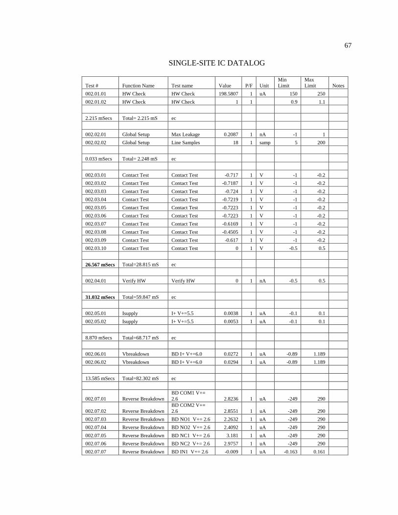
Using the same ATE test system but with a different configuration (Table 2),
device test program written for the IC, and a DIB board designed for the IC were
used to test the different parameters of the DUT IC listed in the datasheet, shown in
Appendix C. Similar to the MOSFET transistor mentioned above, the IC datasheet
also shows the different parameters that are required to test the device. The different
parameters were tested by injecting the stimulus provided by the ATE test system
and the output response is measured in terms of voltage, current, resistance, or time.
These measured values were then compared to the datasheet’s high and low
operational limits to determine a good or defective device. Depending on the
complexity of the IC, these devices can have many more parameters to test than
MOSFET transistors, thereby requiring longer test time. The measurement results
17
were then compiled and reported in a datalog. ‘Dual-Site IC Datalog’ in Appendix
B shows the compiled datalog.
For the Cost of Test study, information including prices of the different
instrumentations, ATE tester, automatic handlers, and other associated costs were
referenced from known databases and equipment manufacturers. Labor rate of
operators and technicians were also referenced from available database and job
board websites.
Data Analysis Procedures
In order to answer the three research questions, a comprehensive data
analysis needed to be performed (Bala, 2005, p.1). For the first research question, a
quantitative comparative analysis of the resulting Final Test (FT) test times of both
the Quad-Site and the Index-Parallel were conducted. The idea behind the Index-
Parallel test methodology is to efficiently use the execution times of the test
procedures of the Multisite (Quad Site) parallel test program by utilizing all idle
times and waiting times, and interleaving the tests procedures to match exactly
without incurring any idle or waiting time. In this way, the program’s total run time
is utilized as close to 100% as possible. This increases the number of devices that
can be tested in a span of 1 hour, or Units per Hour (UPH). Where UPH is
calculated as follows:
Where
18
UPH = Units per Hour,
Ttesttime = Final Test (FT) testtime (ms),
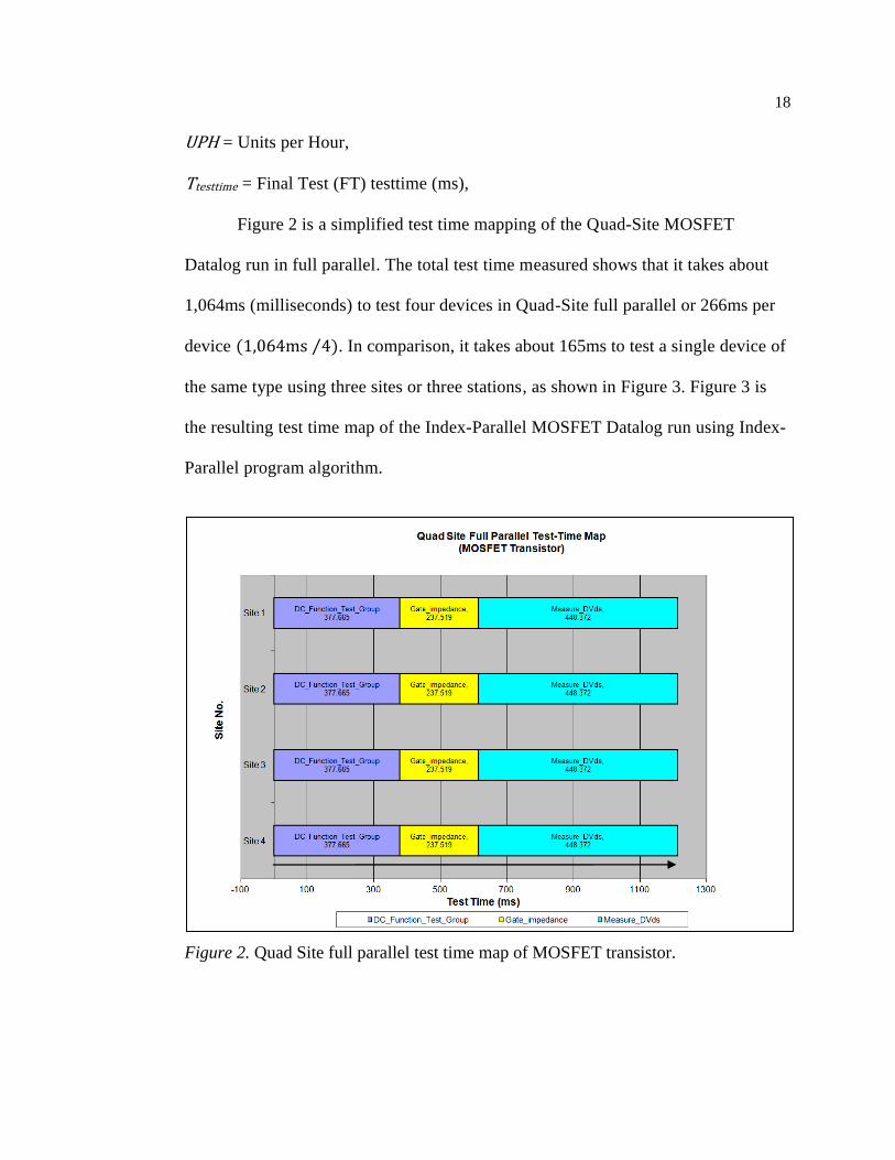
Figure 2 is a simplified test time mapping of the Quad-Site MOSFET
Datalog run in full parallel. The total test time measured shows that it takes about
1,064ms (milliseconds) to test four devices in Quad-Site full parallel or 266ms per
device . In comparison, it takes about 165ms to test a single device of
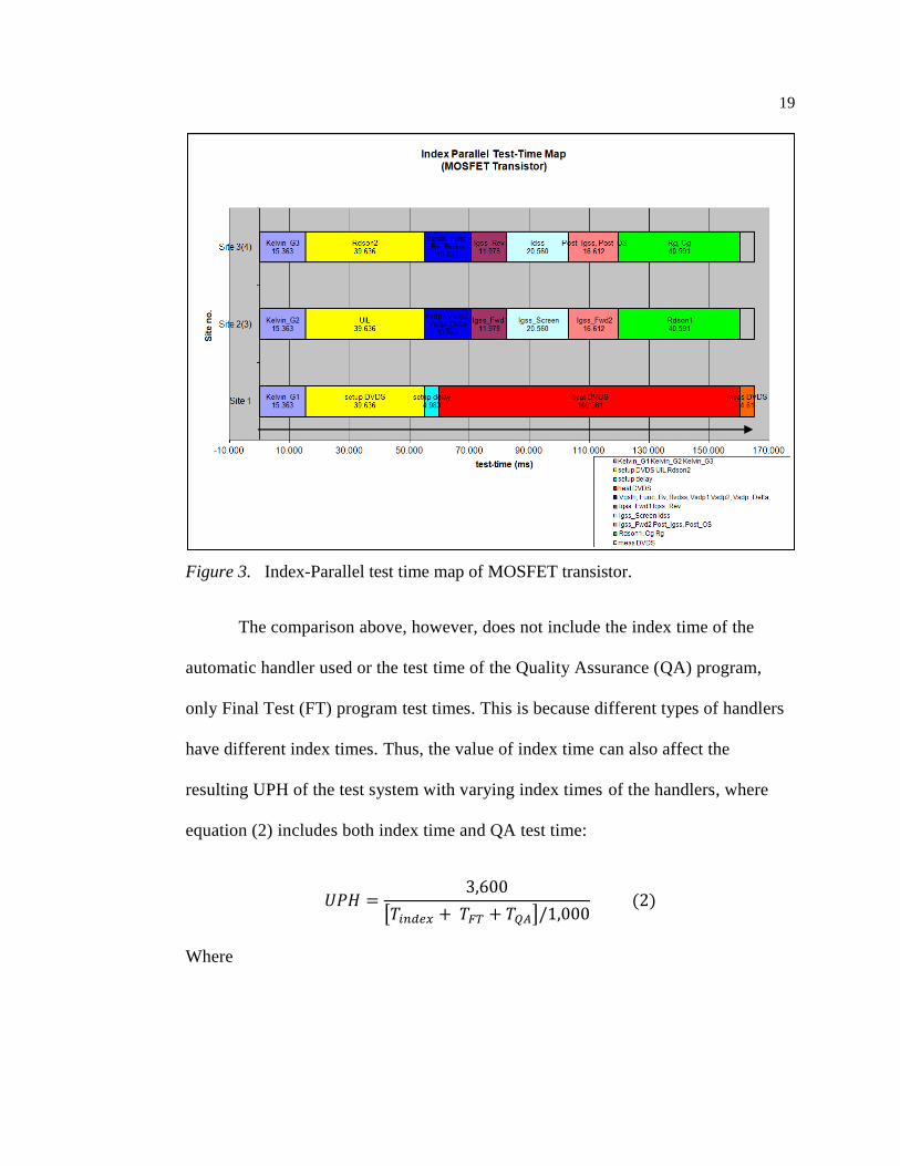
the same type using three sites or three stations, as shown in Figure 3. Figure 3 is
the resulting test time map of the Index-Parallel MOSFET Datalog run using Index-
Parallel program algorithm.
Figure 2. Quad Site full parallel test time map of MOSFET transistor.
19
Figure 3. Index-Parallel test time map of MOSFET transistor.
The comparison above, however, does not include the index time of the
automatic handler used or the test time of the Quality Assurance (QA) program,
only Final Test (FT) program test times. This is because different types of handlers
have different index times. Thus, the value of index time can also affect the
resulting UPH of the test system with varying index times of the handlers, where
equation (2) includes both index time and QA test time:
Where
20
Tindex = handler index time (ms),
TQA = Quality Assurance (QA) test time (ms)
TFT = Final Test (FT) test time (ms)
Ttesttime = Tindex + TFT + TQA (ms).
Automatic handlers are used when large numbers of devices need to be tested in
Production. For the rotary handler, the index time is 120ms and for the Multisite
handler used in the study, the index time is 200ms.
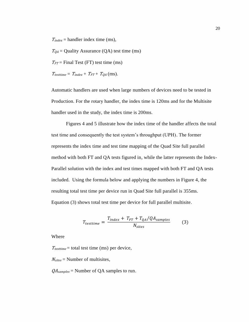
Figures 4 and 5 illustrate how the index time of the handler affects the total
test time and consequently the test system’s throughput (UPH) . The former
represents the index time and test time mapping of the Quad Site full parallel
method with both FT and QA tests figured in, while the latter represents the Index-
Parallel solution with the index and test times mapped with both FT and QA tests
included. Using the formula below and applying the numbers in Figure 4, the
resulting total test time per device run in Quad Site full parallel is 355ms.
Equation (3) shows total test time per device for full parallel multisite.
Where
Ttesttime = total test time (ms) per device,
Nsites = Number of multisites,
QAsamples = Number of QA samples to run.
21
Figure 4. Distribution of test time for FT and QA using Quad-Site parallel testing.
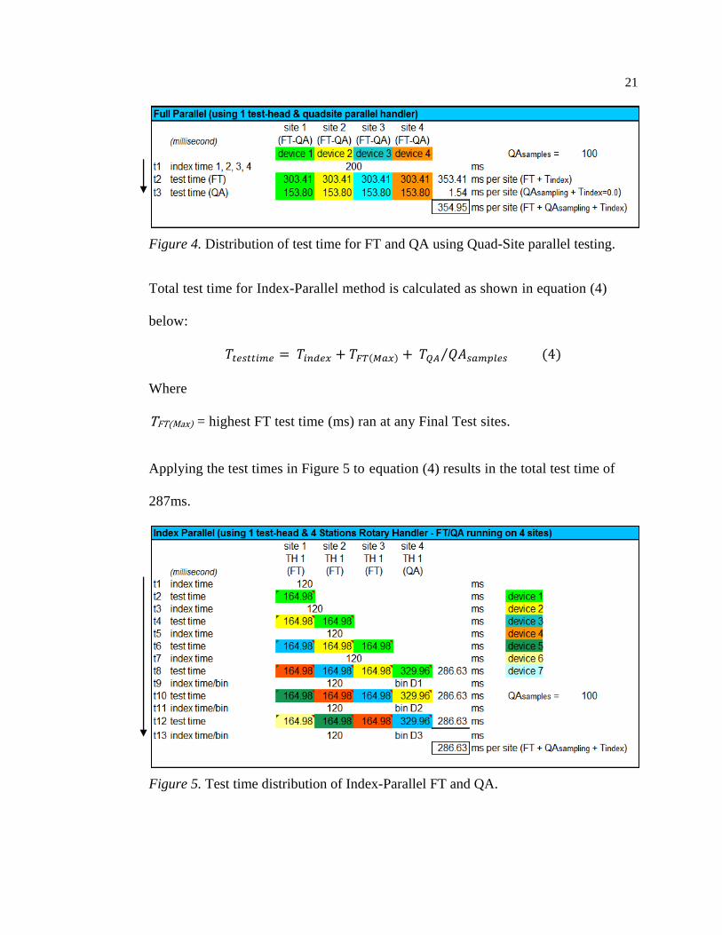
Total test time for Index-Parallel method is calculated as shown in equation (4)
below:
Where
TFT(Max) = highest FT test time (ms) ran at any Final Test sites.
Applying the test times in Figure 5 to equation (4) results in the total test time of
287ms.
Figure 5. Test time distribution of Index-Parallel FT and QA.
22
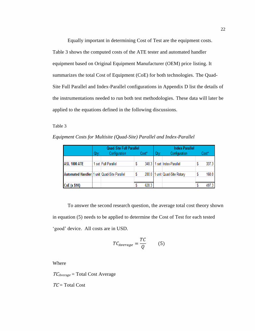
Equally important in determining Cost of Test are the equipment costs.
Table 3 shows the computed costs of the ATE tester and automated handler
equipment based on Original Equipment Manufacturer (OEM) price listing. It
summarizes the total Cost of Equipment (CoE) for both technologies. The Quad-
Site Full Parallel and Index-Parallel configurations in Appendix D list the details of
the instrumentations needed to run both test methodologies. These data will later be
applied to the equations defined in the following discussions.
Table 3
Equipment Costs for Multisite (Quad-Site) Parallel and Index-Parallel
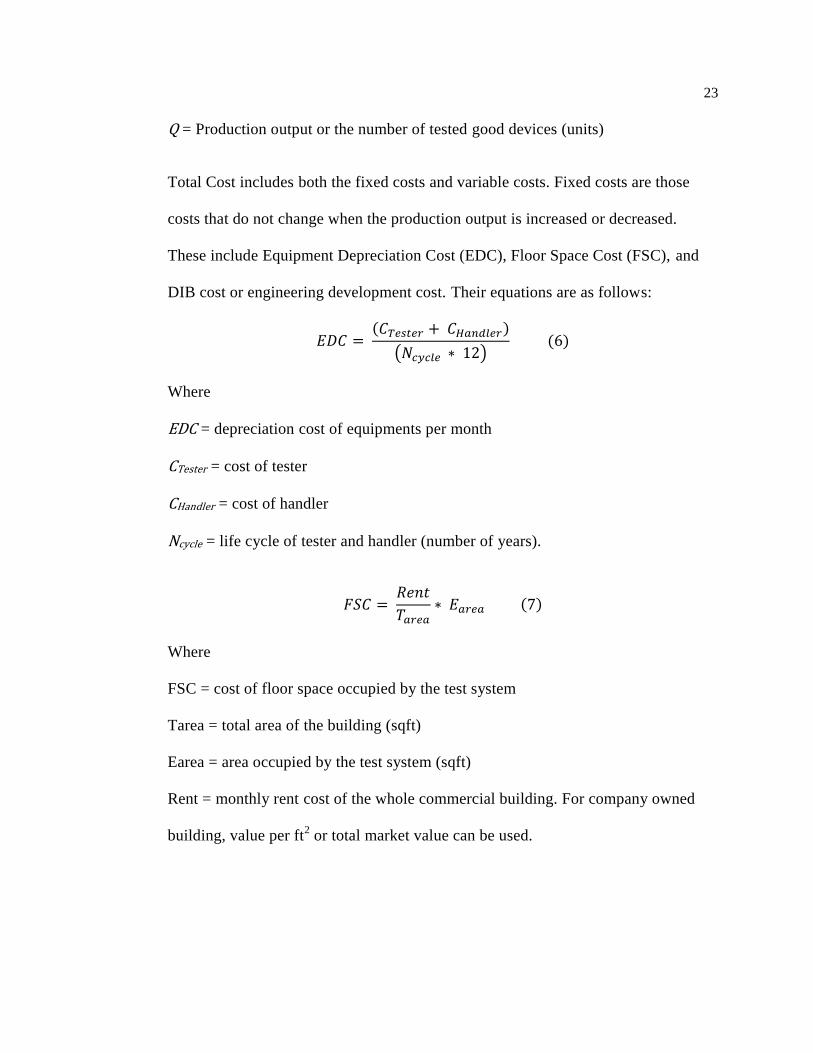
To answer the second research question, the average total cost theory shown
in equation (5) needs to be applied to determine the Cost of Test for each tested
‘good’ device. All costs are in USD.
Where
TCAverage = Total Cost Average
TC = Total Cost
23
Q = Production output or the number of tested good devices (units)
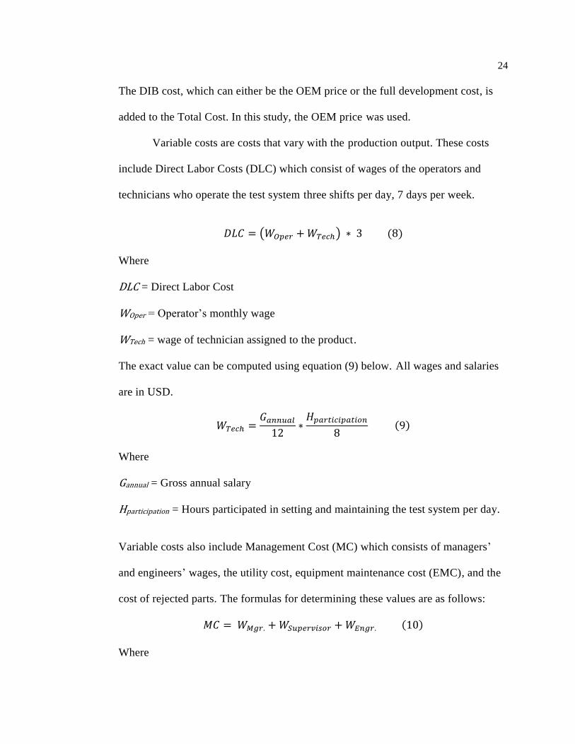
Total Cost includes both the fixed costs and variable costs. Fixed costs are those
costs that do not change when the production output is increased or decreased.
These include Equipment Depreciation Cost (EDC), Floor Space Cost (FSC), and
DIB cost or engineering development cost. Their equations are as follows:
Where
EDC = depreciation cost of equipments per month
CTester = cost of tester
CHandler = cost of handler
Ncycle = life cycle of tester and handler (number of years).
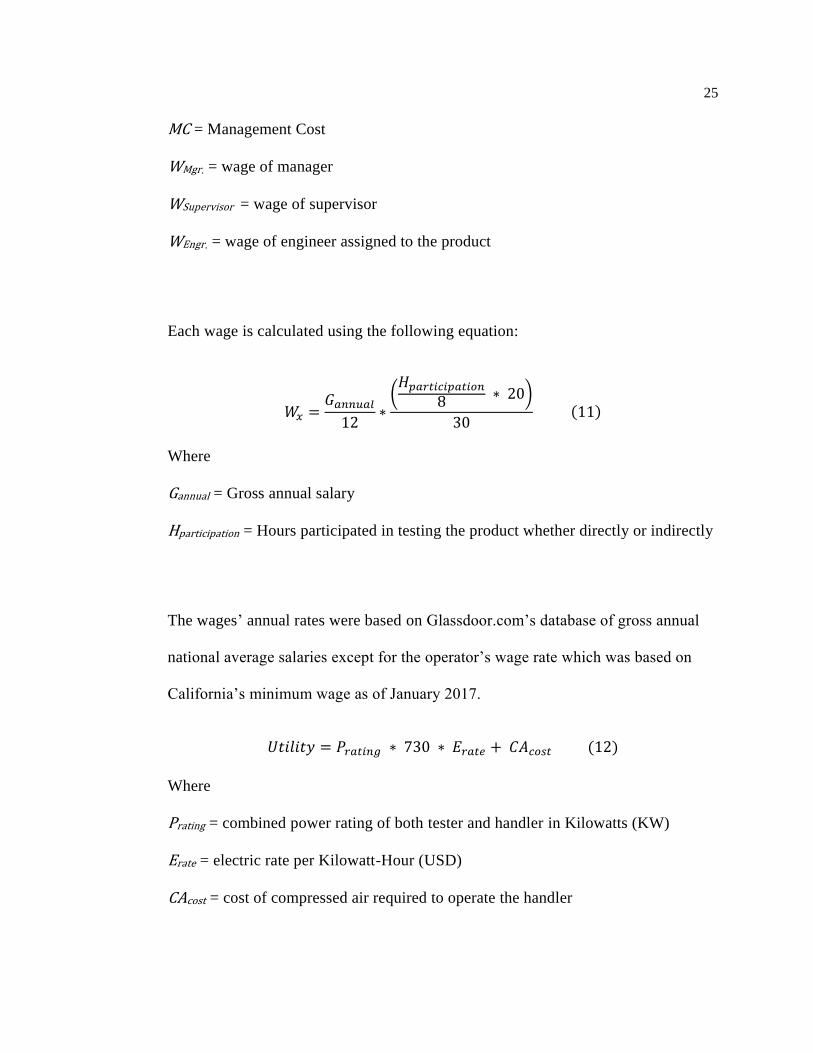
Where
FSC = cost of floor space occupied by the test system
Tarea = total area of the building (sqft)
Earea = area occupied by the test system (sqft)
Rent = monthly rent cost of the whole commercial building. For company owned
building, value per ft2 or total market value can be used.
24
The DIB cost, which can either be the OEM price or the full development cost, is
added to the Total Cost. In this study, the OEM price was used.
Variable costs are costs that vary with the production output. These costs
include Direct Labor Costs (DLC) which consist of wages of the operators and
technicians who operate the test system three shifts per day, 7 days per week.
Where
DLC = Direct Labor Cost
WOper = Operator’s monthly wage
WTech = wage of technician assigned to the product.
The exact value can be computed using equation (9) below. All wages and salaries
are in USD.
Where
Gannual = Gross annual salary
Hparticipation = Hours participated in setting and maintaining the test system per day.
Variable costs also include Management Cost (MC) which consists of managers’
and engineers’ wages, the utility cost, equipment maintenance cost (EMC), and the
cost of rejected parts. The formulas for determining these values are as follows:
Where
25
MC = Management Cost
WMgr. = wage of manager
WSupervisor = wage of supervisor
WEngr. = wage of engineer assigned to the product
Each wage is calculated using the following equation:
Where
Gannual = Gross annual salary
Hparticipation = Hours participated in testing the product whether directly or indirectly
The wages’ annual rates were based on Glassdoor.com’s database of gross annual
national average salaries except for the operator’s wage rate which was based on
California’s minimum wage as of January 2017.
Where
Prating = combined power rating of both tester and handler in Kilowatts (KW)
Erate = electric rate per Kilowatt-Hour (USD)
CAcost = cost of compressed air required to operate the handler
26
Where
EDC = Equipment depreciation cost
M = percentage cost (%)
Finally, it is important to consider the cost of the tested bad devices as part of the
variable cost; this must be added to the total cost (Khoo, 2014).
Where
CRejects = cost of rejects
ASP = Average Selling Price of the device
Lsize = total lot size of untested devices (number of units)
YLDRejects = percentage yield of rejects (%)
Yield is the percentage of good devices tested over the entire lot of untested
devices. It is a measure of the final production output and is computed as equation
(15.1) or (15.2).
Where
YLDGood = percentage yield of tested ‘good’ devices (%)
27
QGood = number of passing or tested ‘good’ devices (number of units)
Once the components of the Average Total Cost are defined, the actual Cost
of Test per device can be determined. UPH for tested good devices is equivalent to
the Output Q and the Total Cost must be converted to the same (per hour) rate as the
UPH. Thus,
Where
UPHGood = Tested good devices per hour
YLDGood = Percentage of good yield (%)
Ttestime = use equation (3) for Multisite full parallel and equation (4) for Index-
Parallel
Where
TCH = Total Cost per Hour
Eusage = Equipment usage or percentage utilization less equipment downtimes (%).
Finally, equations (15) and (16) are applied to equation (5) to get the Average Total
Cost or the Cost of Test per good device.
28
Equations (1) to (18) can be used to calculate throughput and COT when testing
either a transistor or a relatively complex IC device using Multisite or Index-
Parallel technologies.
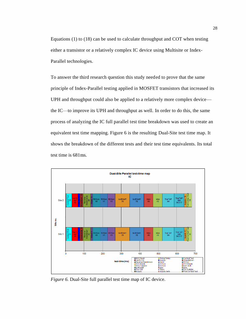
To answer the third research question this study needed to prove that the same
principle of Index-Parallel testing applied in MOSFET transistors that increased its
UPH and throughput could also be applied to a relatively more complex device—
the IC—to improve its UPH and throughput as well. In order to do this, the same
process of analyzing the IC full parallel test time breakdown was used to create an
equivalent test time mapping. Figure 6 is the resulting Dual-Site test time map. It
shows the breakdown of the different tests and their test time equivalents. Its total
test time is 681ms.
Figure 6. Dual-Site full parallel test time map of IC device.
29
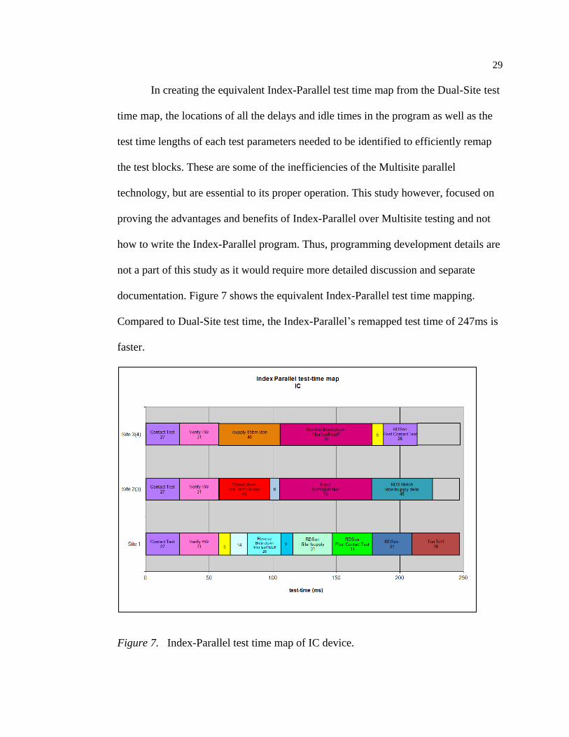
In creating the equivalent Index-Parallel test time map from the Dual-Site test
time map, the locations of all the delays and idle times in the program as well as the
test time lengths of each test parameters needed to be identified to efficiently remap
the test blocks. These are some of the inefficiencies of the Multisite parallel
technology, but are essential to its proper operation. This study however, focused on
proving the advantages and benefits of Index-Parallel over Multisite testing and not
how to write the Index-Parallel program. Thus, programming development details are
not a part of this study as it would require more detailed discussion and separate
documentation. Figure 7 shows the equivalent Index-Parallel test time mapping.
Compared to Dual-Site test time, the Index-Parallel’s remapped test time of 247ms is
faster.
Figure 7. Index-Parallel test time map of IC device.
30
CHAPTER III
RESULTS
Plan of the Study
This study intended to prove the superiority of Index-Parallel technology over
Multisite technology and the benefits that the semiconductor manufacturing can gain
from it. It pointed out the inefficiencies of current Multisite technology and improves
the throughput. It also proved that it can reduce the Cost of Test, making it a viable
solution, and this technology is also applicable to a relatively more complex IC. This
was achieved by implementing the Index-Parallel test methodology and program
algorithm. This study also examined the multivariate analysis of the data to look at
interdependencies of the variables, and applied the principles of Multisite and Index-
Parallel equations of UPH with Average Total Cost theory in calculating the Cost of
Test. This chapter presents the results of the data analysis in answering the three
research questions.
Descriptive Statistics
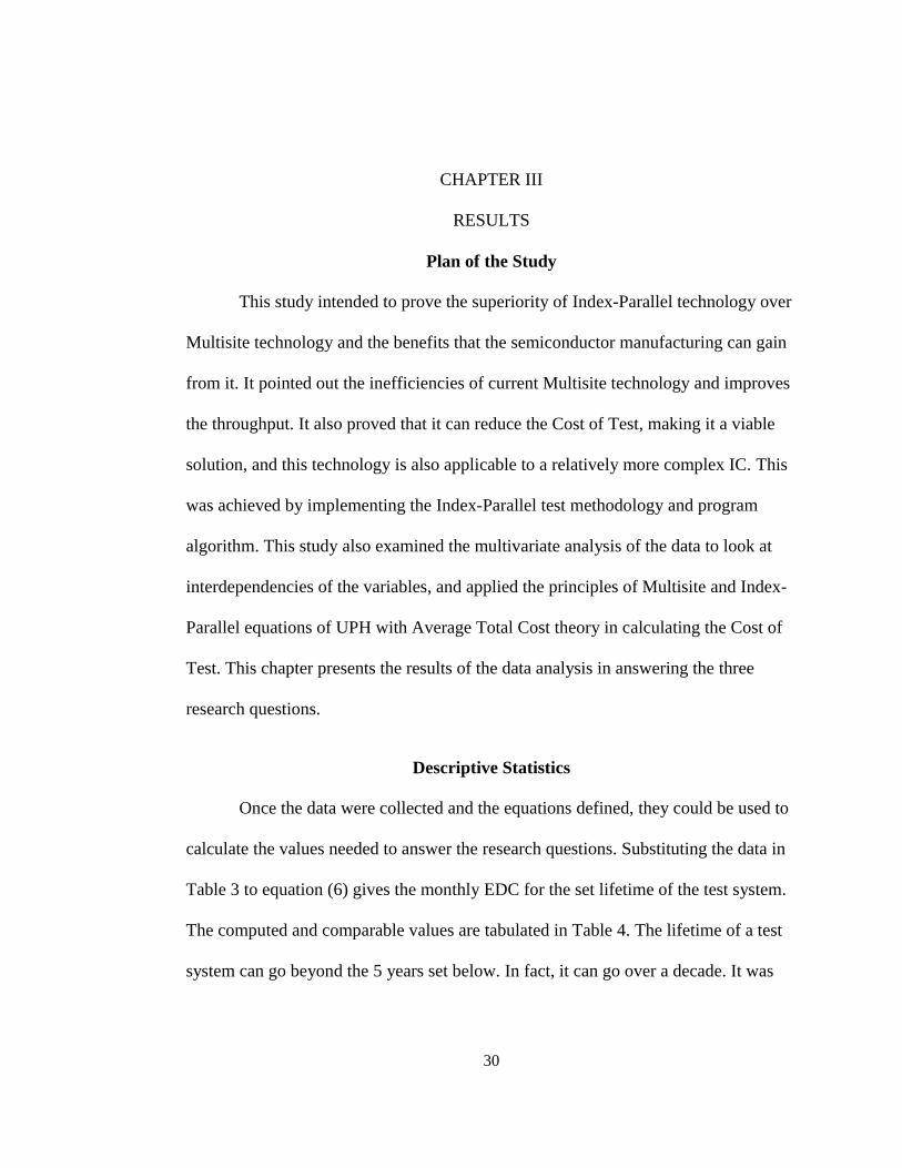
Once the data were collected and the equations defined, they could be used to
calculate the values needed to answer the research questions. Substituting the data in
Table 3 to equation (6) gives the monthly EDC for the set lifetime of the test system.
The computed and comparable values are tabulated in Table 4. The lifetime of a test
system can go beyond the 5 years set below. In fact, it can go over a decade. It was
31
set to five because the forecasted total saved can recover the amount invested in the
test system in less than 5 years.
Table 4
Monthly Equipment Depreciation Costs Comparison
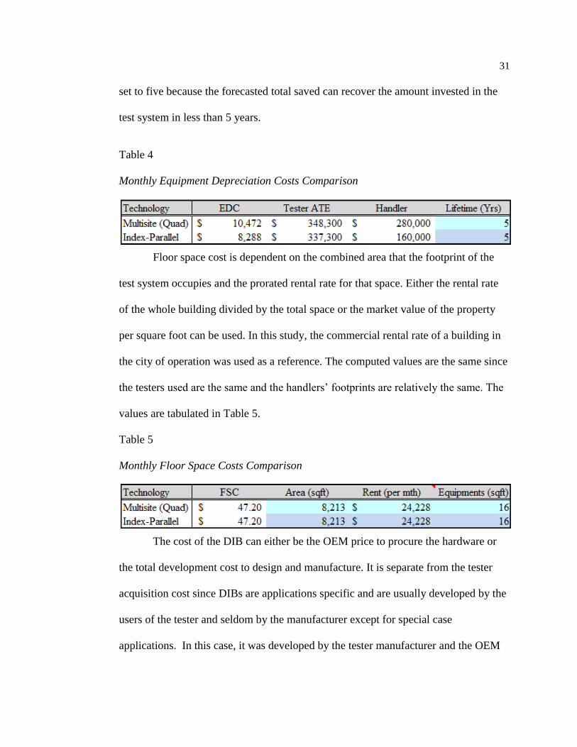
Floor space cost is dependent on the combined area that the footprint of the
test system occupies and the prorated rental rate for that space. Either the rental rate
of the whole building divided by the total space or the market value of the property
per square foot can be used. In this study, the commercial rental rate of a building in
the city of operation was used as a reference. The computed values are the same since
the testers used are the same and the handlers’ footprints are relatively the same. The
values are tabulated in Table 5.
Table 5
Monthly Floor Space Costs Comparison
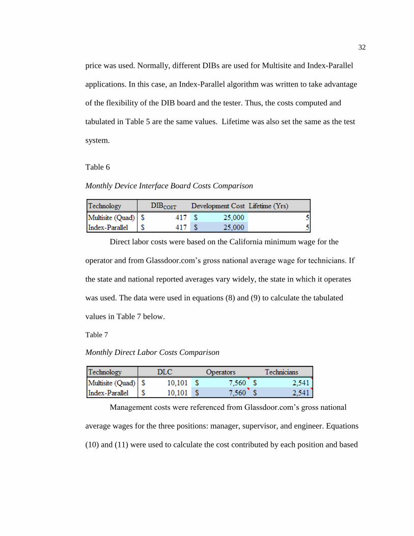
The cost of the DIB can either be the OEM price to procure the hardware or
the total development cost to design and manufacture. It is separate from the tester
acquisition cost since DIBs are applications specific and are usually developed by the
users of the tester and seldom by the manufacturer except for special case
applications. In this case, it was developed by the tester manufacturer and the OEM
32
price was used. Normally, different DIBs are used for Multisite and Index-Parallel
applications. In this case, an Index-Parallel algorithm was written to take advantage
of the flexibility of the DIB board and the tester. Thus, the costs computed and
tabulated in Table 5 are the same values. Lifetime was also set the same as the test
system.
Table 6
Monthly Device Interface Board Costs Comparison
Direct labor costs were based on the California minimum wage for the
operator and from Glassdoor.com’s gross national average wage for technicians. If
the state and national reported averages vary widely, the state in which it operates
was used. The data were used in equations (8) and (9) to calculate the tabulated
values in Table 7 below.
Table 7
Monthly Direct Labor Costs Comparison
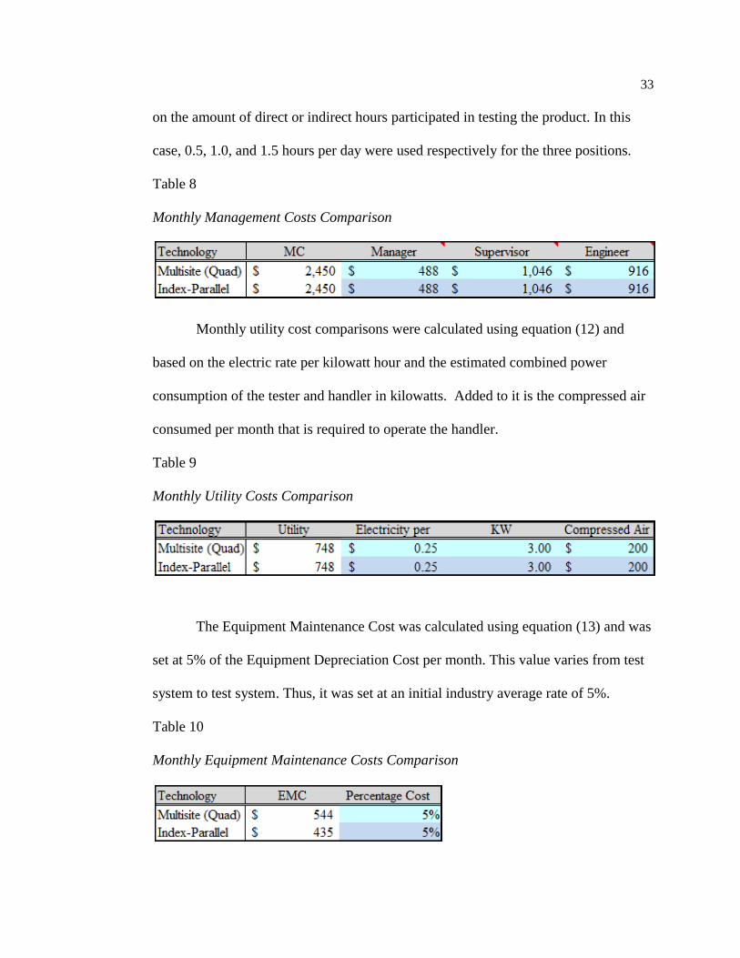
Management costs were referenced from Glassdoor.com’s gross national
average wages for the three positions: manager, supervisor, and engineer. Equations
(10) and (11) were used to calculate the cost contributed by each position and based
33
on the amount of direct or indirect hours participated in testing the product. In this
case, 0.5, 1.0, and 1.5 hours per day were used respectively for the three positions.
Table 8
Monthly Management Costs Comparison
Monthly utility cost comparisons were calculated using equation (12) and
based on the electric rate per kilowatt hour and the estimated combined power
consumption of the tester and handler in kilowatts. Added to it is the compressed air
consumed per month that is required to operate the handler.
Table 9
Monthly Utility Costs Comparison
The Equipment Maintenance Cost was calculated using equation (13) and was
set at 5% of the Equipment Depreciation Cost per month. This value varies from test
system to test system. Thus, it was set at an initial industry average rate of 5%.
Table 10
Monthly Equipment Maintenance Costs Comparison
34
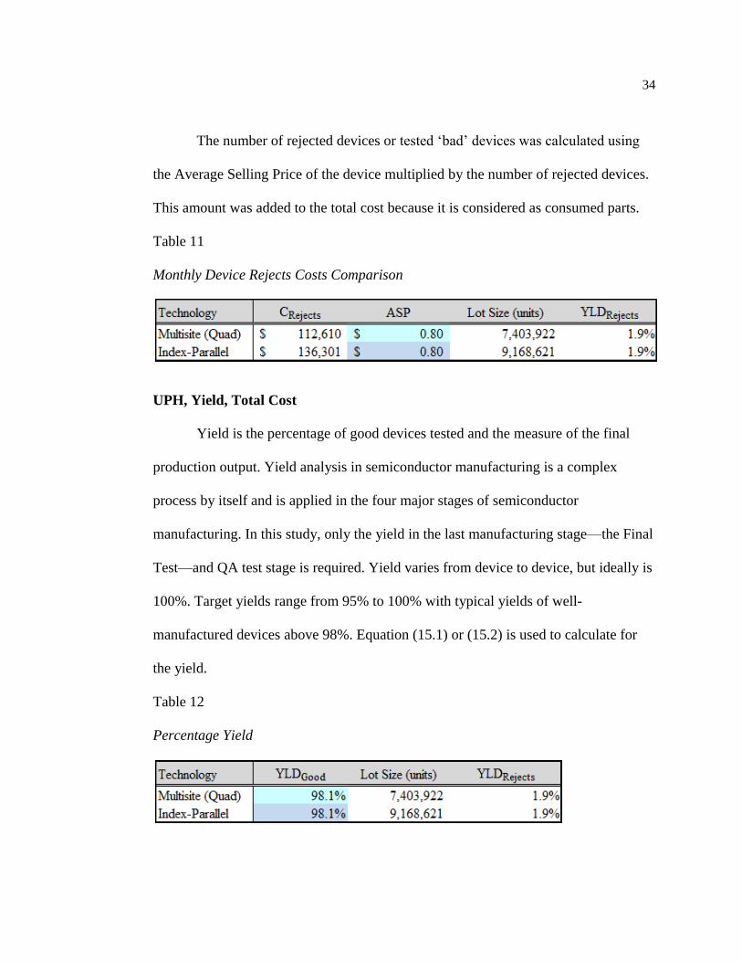
The number of rejected devices or tested ‘bad’ devices was calculated using
the Average Selling Price of the device multiplied by the number of rejected devices.
This amount was added to the total cost because it is considered as consumed parts.
Table 11
Monthly Device Rejects Costs Comparison
UPH, Yield, Total Cost
Yield is the percentage of good devices tested and the measure of the final
production output. Yield analysis in semiconductor manufacturing is a complex
process by itself and is applied in the four major stages of semiconductor
manufacturing. In this study, only the yield in the last manufacturing stage—the Final
Test—and QA test stage is required. Yield varies from device to device, but ideally is
100%. Target yields range from 95% to 100% with typical yields of well-
manufactured devices above 98%. Equation (15.1) or (15.2) is used to calculate for
the yield.
Table 12
Percentage Yield
35
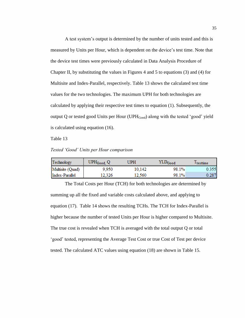
A test system’s output is determined by the number of units tested and this is
measured by Units per Hour, which is dependent on the device’s test time. Note that
the device test times were previously calculated in Data Analysis Procedure of
Chapter II, by substituting the values in Figures 4 and 5 to equations (3) and (4) for
Multisite and Index-Parallel, respectively. Table 13 shows the calculated test time
values for the two technologies. The maximum UPH for both technologies are
calculated by applying their respective test times to equation (1). Subsequently, the
output Q or tested good Units per Hour (UPHGood) along with the tested ‘good’ yield
is calculated using equation (16).
Table 13
Tested ‘Good’ Units per Hour comparison
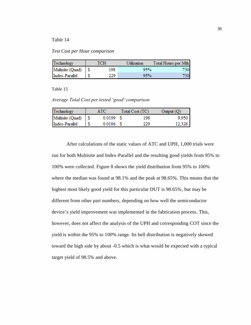
The Total Costs per Hour (TCH) for both technologies are determined by
summing up all the fixed and variable costs calculated above, and applying to
equation (17). Table 14 shows the resulting TCHs. The TCH for Index-Parallel is
higher because the number of tested Units per Hour is higher compared to Multisite.
The true cost is revealed when TCH is averaged with the total output Q or total
‘good’ tested, representing the Average Test Cost or true Cost of Test per device
tested. The calculated ATC values using equation (18) are shown in Table 15.
36
Table 14
Test Cost per Hour comparison
Table 15
Average Total Cost per tested ‘good’ comparison
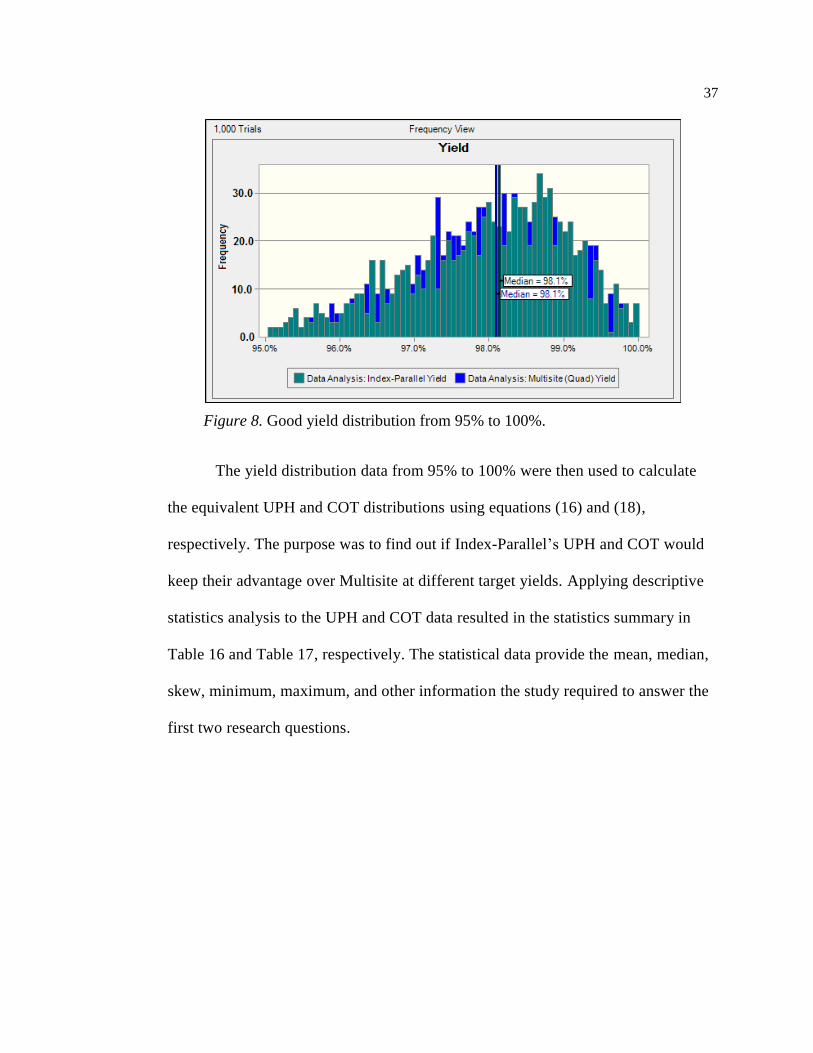
After calculations of the static values of ATC and UPH, 1,000 trials were
run for both Multisite and Index-Parallel and the resulting good yields from 95% to
100% were collected. Figure 8 shows the yield distribution from 95% to 100%
where the median was found at 98.1% and the peak at 98.65%. This means that the
highest most likely good yield for this particular DUT is 98.65%, but may be
different from other part numbers, depending on how well the semiconductor
device’s yield improvement was implemented in the fabrication process. This,
however, does not affect the analysis of the UPH and corresponding COT since the
yield is within the 95% to 100% range. Its bell distribution is negatively skewed
toward the high side by about -0.5 which is what would be expected with a typical
target yield of 98.5% and above.
37
Figure 8. Good yield distribution from 95% to 100%.
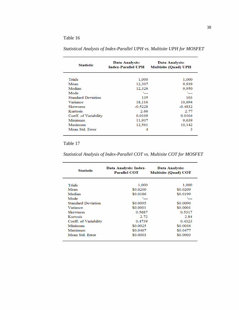
The yield distribution data from 95% to 100% were then used to calculate
the equivalent UPH and COT distributions using equations (16) and (18),
respectively. The purpose was to find out if Index-Parallel’s UPH and COT would
keep their advantage over Multisite at different target yields. Applying descriptive
statistics analysis to the UPH and COT data resulted in the statistics summary in
Table 16 and Table 17, respectively. The statistical data provide the mean, median,
skew, minimum, maximum, and other information the study required to answer the
first two research questions.
38
Table 16
Statistical Analysis of Index-Parallel UPH vs. Multisite UPH for MOSFET
Table 17
Statistical Analysis of Index-Parallel COT vs. Multisite COT for MOSFET
39
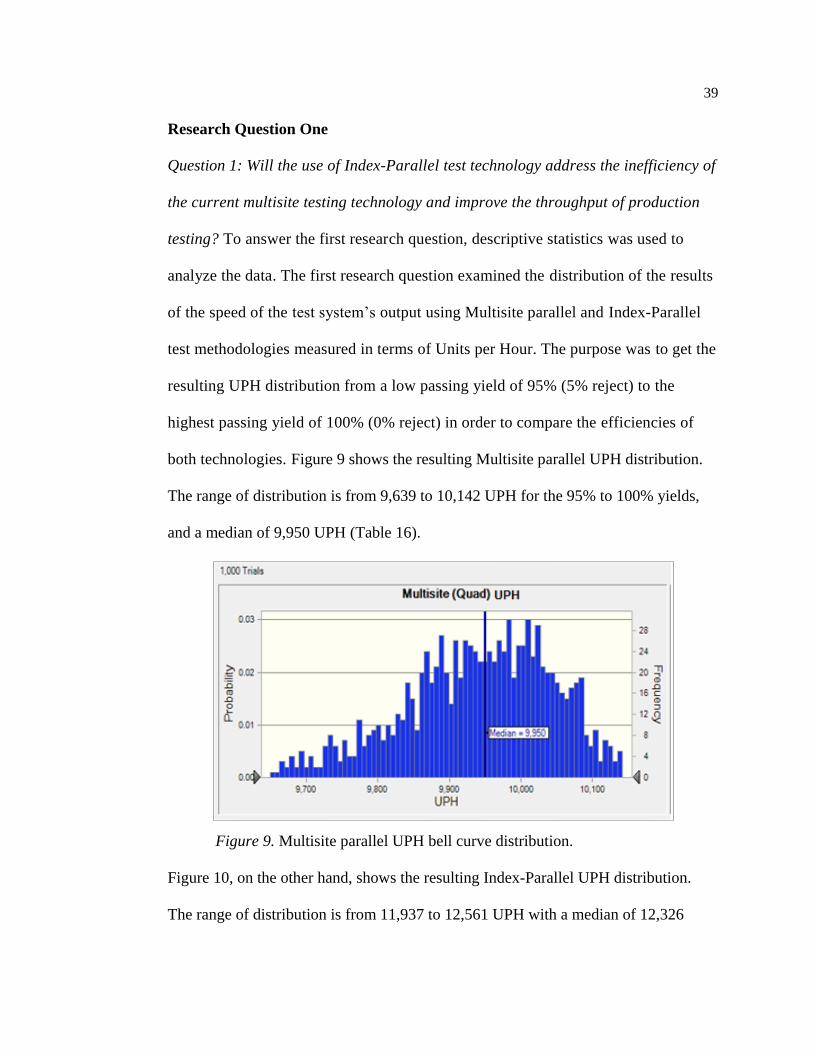
Research Question One
Question 1: Will the use of Index-Parallel test technology address the inefficiency of
the current multisite testing technology and improve the throughput of production
testing? To answer the first research question, descriptive statistics was used to
analyze the data. The first research question examined the distribution of the results
of the speed of the test system’s output using Multisite parallel and Index-Parallel
test methodologies measured in terms of Units per Hour. The purpose was to get the
resulting UPH distribution from a low passing yield of 95% (5% reject) to the
highest passing yield of 100% (0% reject) in order to compare the efficiencies of
both technologies. Figure 9 shows the resulting Multisite parallel UPH distribution.
The range of distribution is from 9,639 to 10,142 UPH for the 95% to 100% yields,
and a median of 9,950 UPH (Table 16).
Figure 9. Multisite parallel UPH bell curve distribution.
Figure 10, on the other hand, shows the resulting Index-Parallel UPH distribution.
The range of distribution is from 11,937 to 12,561 UPH with a median of 12,326
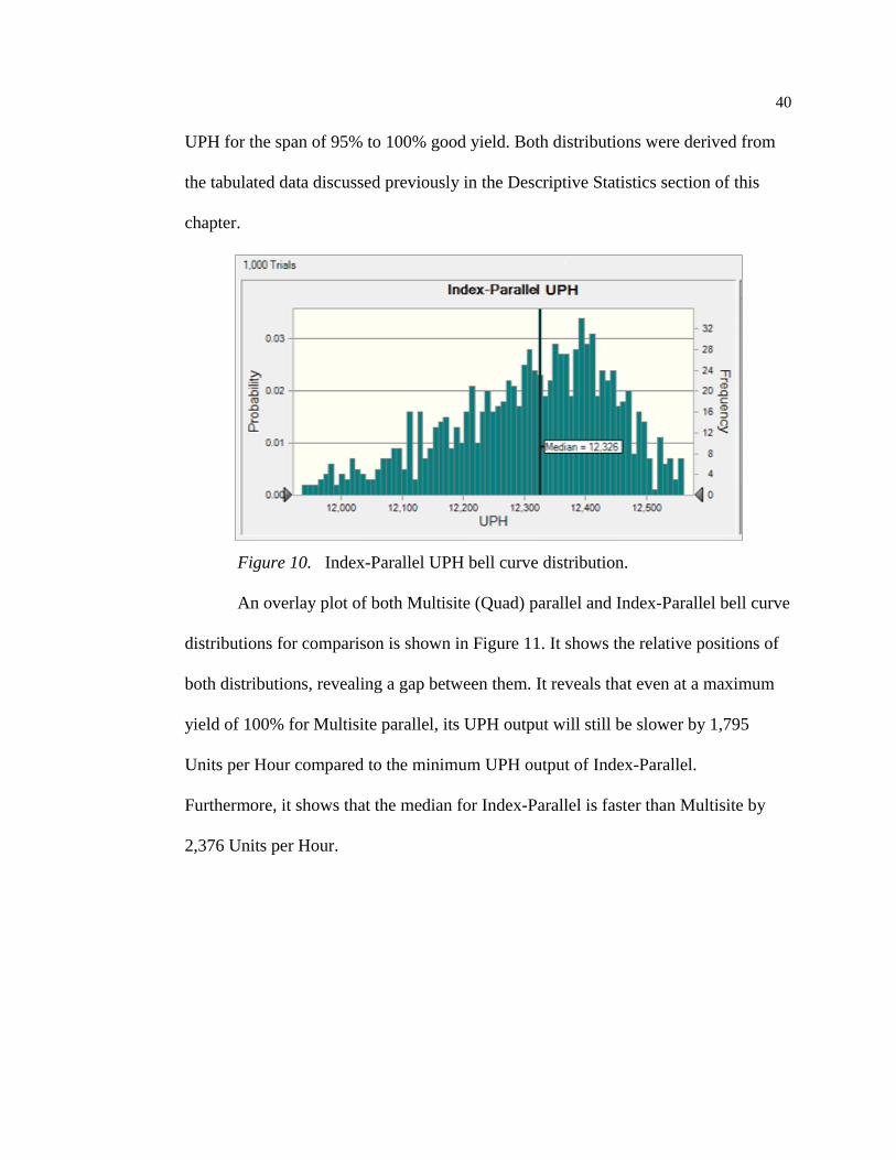
40
UPH for the span of 95% to 100% good yield. Both distributions were derived from
the tabulated data discussed previously in the Descriptive Statistics section of this
chapter.
Figure 10. Index-Parallel UPH bell curve distribution.
An overlay plot of both Multisite (Quad) parallel and Index-Parallel bell curve
distributions for comparison is shown in Figure 11. It shows the relative positions of
both distributions, revealing a gap between them. It reveals that even at a maximum
yield of 100% for Multisite parallel, its UPH output will still be slower by 1,795
Units per Hour compared to the minimum UPH output of Index-Parallel.
Furthermore, it shows that the median for Index-Parallel is faster than Multisite by
2,376 Units per Hour.
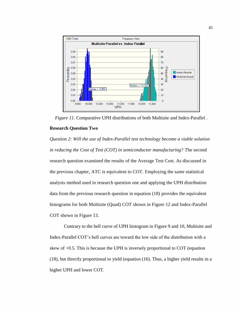
41
Figure 11. Comparative UPH distributions of both Multisite and Index-Parallel .
Research Question Two
Question 2: Will the use of Index-Parallel test technology become a viable solution
in reducing the Cost of Test (COT) in semiconductor manufacturing? The second
research question examined the results of the Average Test Cost. As discussed in
the previous chapter, ATC is equivalent to COT. Employing the same statistical
analysis method used in research question one and applying the UPH distribution
data from the previous research question in equation (18) provides the equivalent
histograms for both Multisite (Quad) COT shown in Figure 12 and Index-Parallel
COT shown in Figure 13.
Contrary to the bell curve of UPH histogram in Figure 9 and 10, Multisite and
Index-Parallel COT’s bell curves are toward the low side of the distribution with a
skew of +0.5. This is because the UPH is inversely proportional to COT (equation
(18), but directly proportional to yield (equation (16). Thus, a higher yield results in a
higher UPH and lower COT.
42
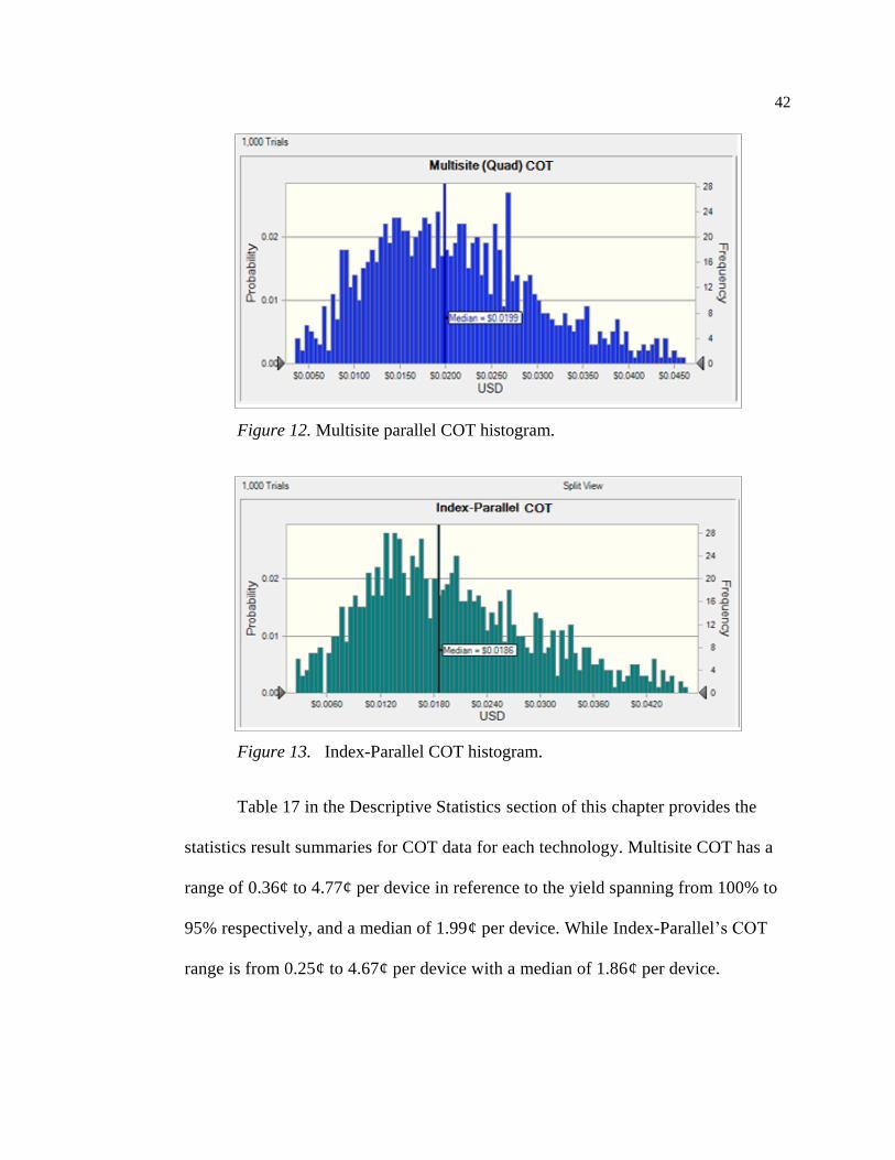
Figure 12. Multisite parallel COT histogram.
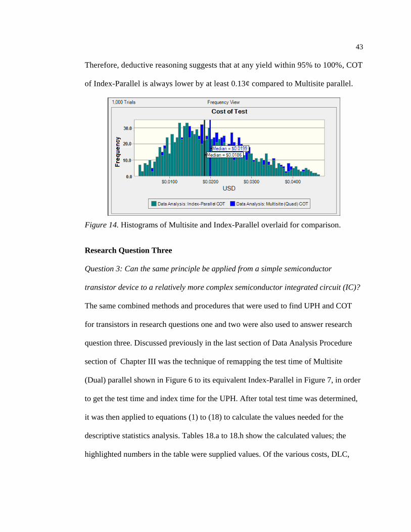
Figure 13. Index-Parallel COT histogram.
Table 17 in the Descriptive Statistics section of this chapter provides the
statistics result summaries for COT data for each technology. Multisite COT has a
range of 0.36¢ to 4.77¢ per device in reference to the yield spanning from 100% to
95% respectively, and a median of 1.99¢ per device. While Index-Parallel’s COT
range is from 0.25¢ to 4.67¢ per device with a median of 1.86¢ per device.
43
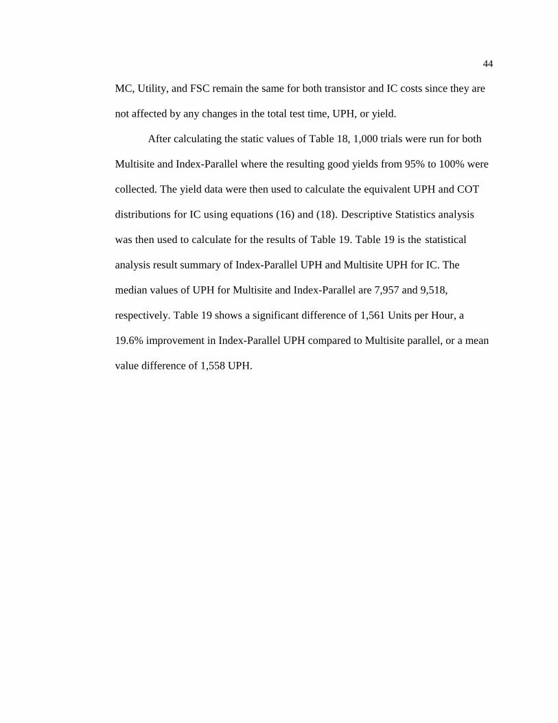
Therefore, deductive reasoning suggests that at any yield within 95% to 100%, COT
of Index-Parallel is always lower by at least 0.13¢ compared to Multisite parallel.
Figure 14. Histograms of Multisite and Index-Parallel overlaid for comparison.
Research Question Three
Question 3: Can the same principle be applied from a simple semiconductor
transistor device to a relatively more complex semiconductor integrated circuit (IC)?
The same combined methods and procedures that were used to find UPH and COT
for transistors in research questions one and two were also used to answer research
question three. Discussed previously in the last section of Data Analysis Procedure
section of Chapter III was the technique of remapping the test time of Multisite
(Dual) parallel shown in Figure 6 to its equivalent Index-Parallel in Figure 7, in order
to get the test time and index time for the UPH. After total test time was determined,
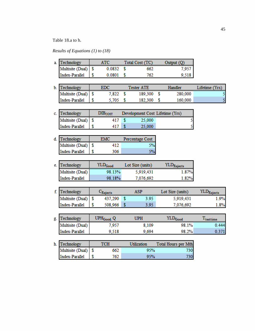
it was then applied to equations (1) to (18) to calculate the values needed for the
descriptive statistics analysis. Tables 18.a to 18.h show the calculated values; the
highlighted numbers in the table were supplied values. Of the various costs, DLC,
44
MC, Utility, and FSC remain the same for both transistor and IC costs since they are
not affected by any changes in the total test time, UPH, or yield.
After calculating the static values of Table 18, 1,000 trials were run for both
Multisite and Index-Parallel where the resulting good yields from 95% to 100% were
collected. The yield data were then used to calculate the equivalent UPH and COT
distributions for IC using equations (16) and (18). Descriptive Statistics analysis
was then used to calculate for the results of Table 19. Table 19 is the statistical
analysis result summary of Index-Parallel UPH and Multisite UPH for IC. The
median values of UPH for Multisite and Index-Parallel are 7,957 and 9,518,
respectively. Table 19 shows a significant difference of 1,561 Units per Hour, a
19.6% improvement in Index-Parallel UPH compared to Multisite parallel, or a mean
value difference of 1,558 UPH.
45
Table 18.a to h.
Results of Equations (1) to (18)
46
Table 19
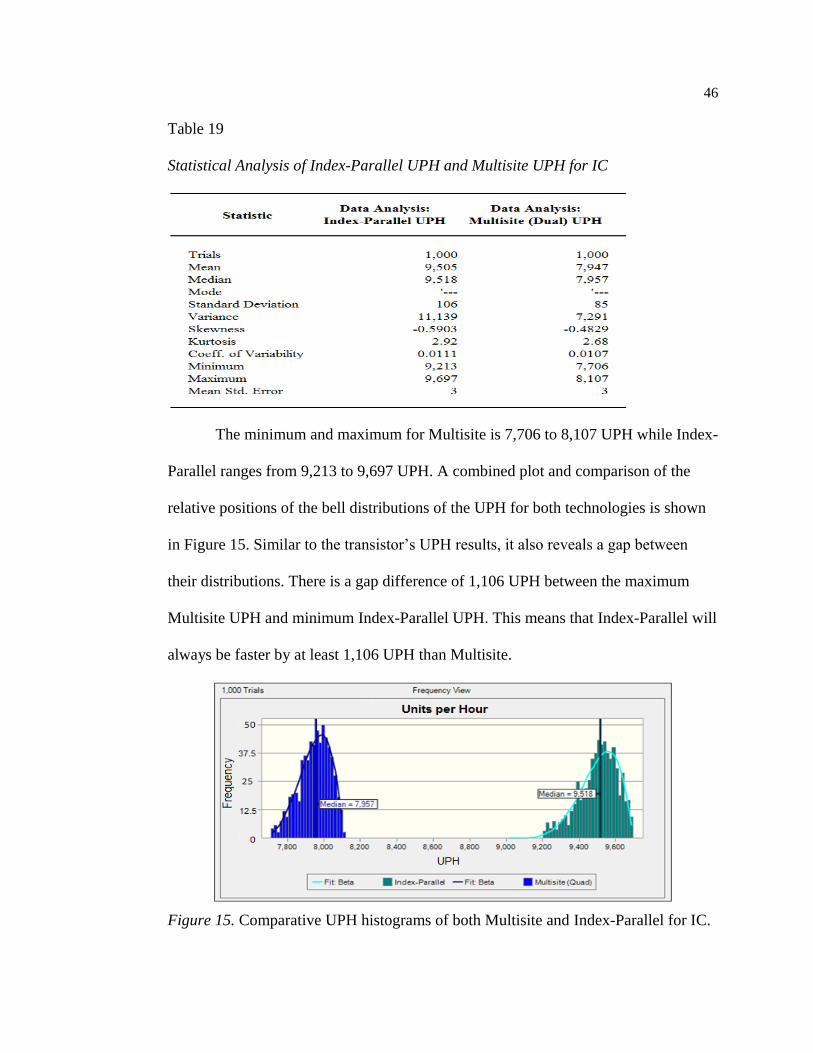
Statistical Analysis of Index-Parallel UPH and Multisite UPH for IC
The minimum and maximum for Multisite is 7,706 to 8,107 UPH while Index-
Parallel ranges from 9,213 to 9,697 UPH. A combined plot and comparison of the
relative positions of the bell distributions of the UPH for both technologies is shown
in Figure 15. Similar to the transistor’s UPH results, it also reveals a gap between
their distributions. There is a gap difference of 1,106 UPH between the maximum
Multisite UPH and minimum Index-Parallel UPH. This means that Index-Parallel will
always be faster by at least 1,106 UPH than Multisite.
Figure 15. Comparative UPH histograms of both Multisite and Index-Parallel for IC.
47
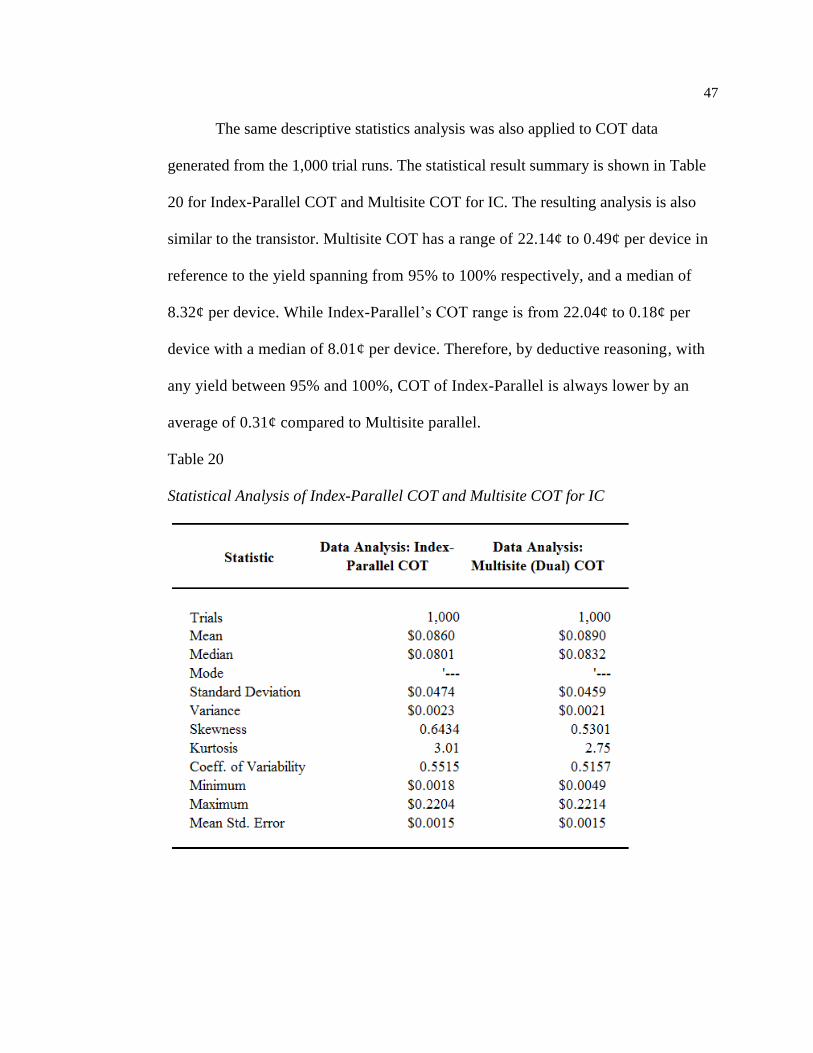
The same descriptive statistics analysis was also applied to COT data
generated from the 1,000 trial runs. The statistical result summary is shown in Table
20 for Index-Parallel COT and Multisite COT for IC. The resulting analysis is also
similar to the transistor. Multisite COT has a range of 22.14¢ to 0.49¢ per device in
reference to the yield spanning from 95% to 100% respectively, and a median of
8.32¢ per device. While Index-Parallel’s COT range is from 22.04¢ to 0.18¢ per
device with a median of 8.01¢ per device. Therefore, by deductive reasoning, with
any yield between 95% and 100%, COT of Index-Parallel is always lower by an
average of 0.31¢ compared to Multisite parallel.
Table 20
Statistical Analysis of Index-Parallel COT and Multisite COT for IC
48
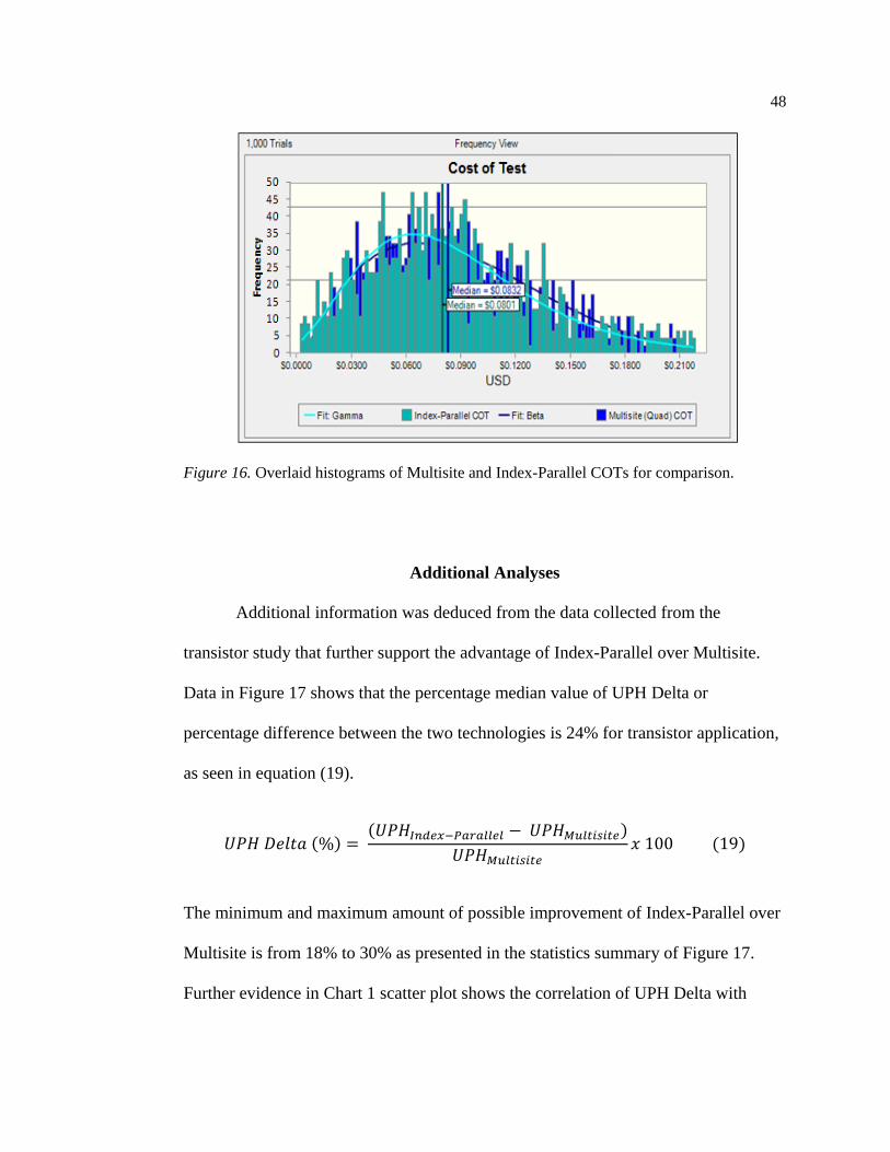
Figure 16. Overlaid histograms of Multisite and Index-Parallel COTs for comparison.
Additional Analyses
Additional information was deduced from the data collected from the
transistor study that further support the advantage of Index-Parallel over Multisite.
Data in Figure 17 shows that the percentage median value of UPH Delta or
percentage difference between the two technologies is 24% for transistor application,
as seen in equation (19).
The minimum and maximum amount of possible improvement of Index-Parallel over
Multisite is from 18% to 30% as presented in the statistics summary of Figure 17.
Further evidence in Chart 1 scatter plot shows the correlation of UPH Delta with
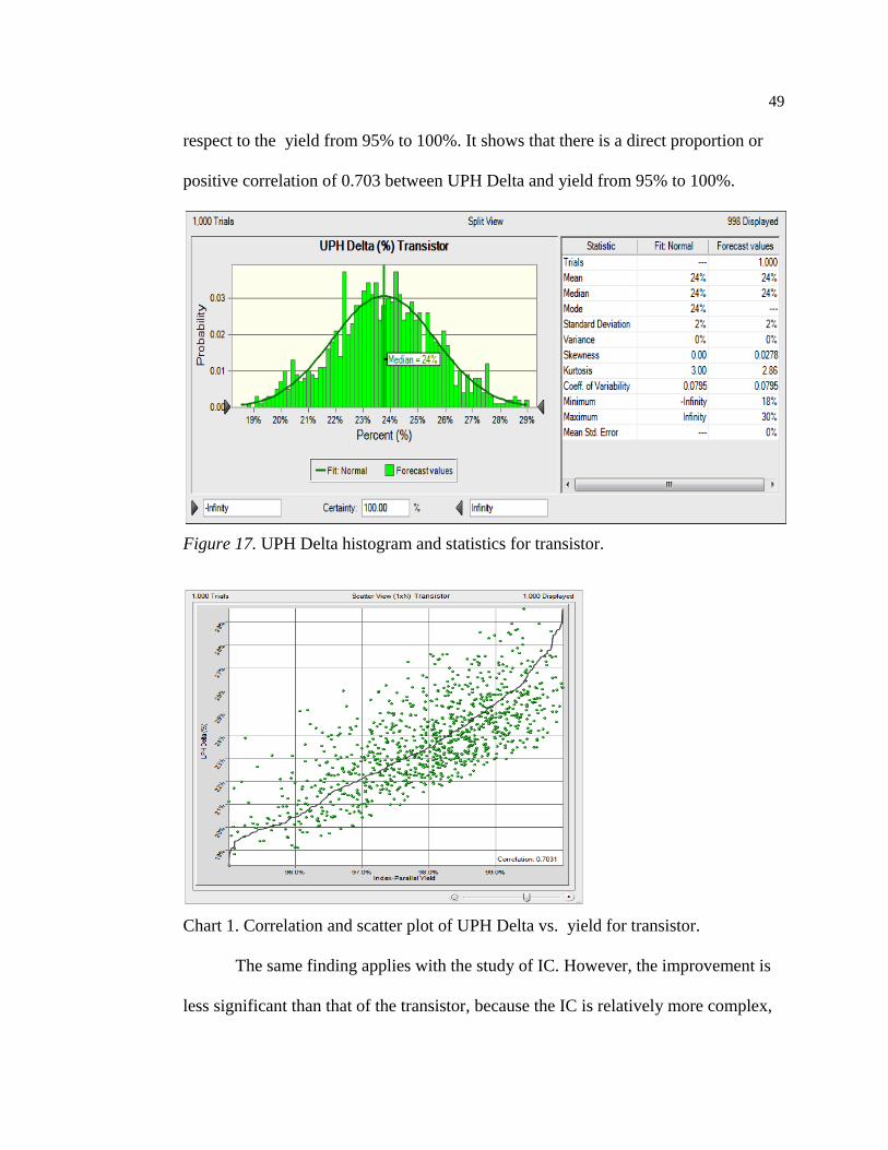
49
respect to the yield from 95% to 100%. It shows that there is a direct proportion or
positive correlation of 0.703 between UPH Delta and yield from 95% to 100%.
Figure 17. UPH Delta histogram and statistics for transistor.
Chart 1. Correlation and scatter plot of UPH Delta vs. yield for transistor.
The same finding applies with the study of IC. However, the improvement is
less significant than that of the transistor, because the IC is relatively more complex,
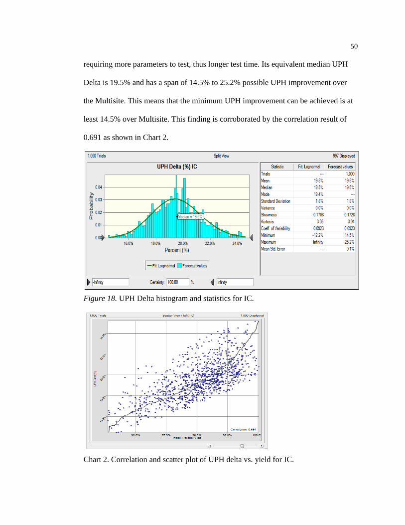
50
requiring more parameters to test, thus longer test time. Its equivalent median UPH
Delta is 19.5% and has a span of 14.5% to 25.2% possible UPH improvement over
the Multisite. This means that the minimum UPH improvement can be achieved is at
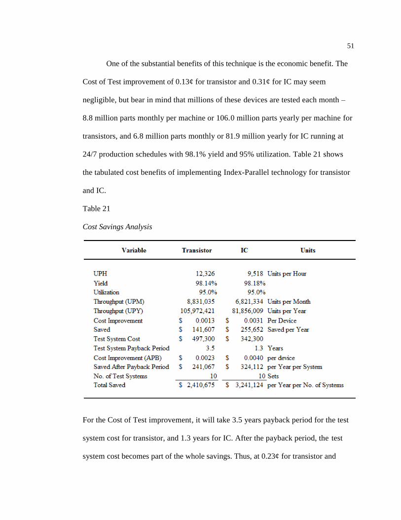
least 14.5% over Multisite. This finding is corroborated by the correlation result of
0.691 as shown in Chart 2.
Figure 18. UPH Delta histogram and statistics for IC.
Chart 2. Correlation and scatter plot of UPH delta vs. yield for IC.
51
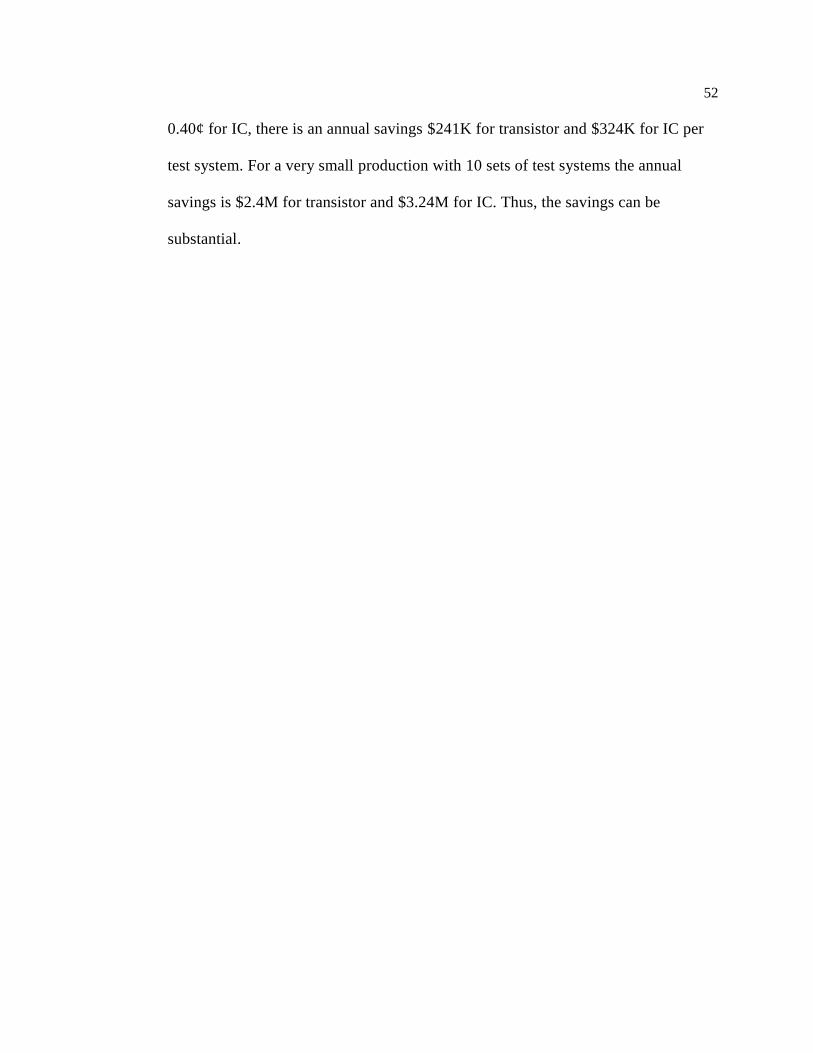
One of the substantial benefits of this technique is the economic benefit. The
Cost of Test improvement of 0.13¢ for transistor and 0.31¢ for IC may seem
negligible, but bear in mind that millions of these devices are tested each month –
8.8 million parts monthly per machine or 106.0 million parts yearly per machine for
transistors, and 6.8 million parts monthly or 81.9 million yearly for IC running at
24/7 production schedules with 98.1% yield and 95% utilization. Table 21 shows
the tabulated cost benefits of implementing Index-Parallel technology for transistor
and IC.
Table 21
Cost Savings Analysis
For the Cost of Test improvement, it will take 3.5 years payback period for the test
system cost for transistor, and 1.3 years for IC. After the payback period, the test
system cost becomes part of the whole savings. Thus, at 0.23¢ for transistor and
52
0.40¢ for IC, there is an annual savings $241K for transistor and $324K for IC per
test system. For a very small production with 10 sets of test systems the annual
savings is $2.4M for transistor and $3.24M for IC. Thus, the savings can be
substantial.
53
CHAPTER IV
DISCUSSION, RECOMMENDATIONS, AND CONCLUSIONS
Discussion of the Findings
Research Question One
Will the use of Index-Parallel test technology address the inefficiency of the
current multisite testing technology and improve the throughput of production
testing?
The findings regarding research question one supported the claim that Index-
Parallel improved production throughput and subsequently addressed Multisite
inefficiency. The resulting increase in UPH brought about by using the Index-
Parallel’s efficient method of remapping Multisite test times increased the test
system’s output. Spanning the test run over the acceptable and target yield from 95%
to 100% consistently produced an average increase in output speed of 2,376 Units per
Hour over Multisite.
Total test time, UPH, good yield, and reject yield are the key variables in
determining the test system’s throughput. Although the other 34 factors were part of
the calculations, they do not directly affect the throughput as much as the four
variables mentioned above. However, reject yield had the opposite effect on
throughput compared to total test time, UPH, and good yield because reject yield is
inversely proportional to the throughput.
54
Research Question Two
Will the use of Index-Parallel test technology become a viable solution in
reducing the Cost of Test (COT) in semiconductor manufacturing?
The resulting Cost of Test or Average Total Cost difference between Index-
Parallel and Multisite is 0.13¢ for transistor and 0.31¢ for IC. These reduced COT
per device in Index-Parallel compared to the current Multisite standard proves that
Index-Parallel technology is a viable solution in reducing COT in semiconductor
manufacturing. Similar to throughput, COT is also directly affected by total test
time, UPH, good yield, and reject yield. But, unlike throughput, yield is also
affected by the total cost of all fixed and variable costs (EDC, FSC, DLC, MC, DIB,
Utility, EMC, and cost of rejected parts). Lowering any of these fixed and variable
costs can have an effect on COT, but not as significant as the four variables which
directly affect the production output and subsequently COT (effect of UPH is
discussed in research question one above). The Index-Parallel technology directly
altered and improved total test time and UPH. The other variable related to yield
(good and reject) can only be improved by engineering analysis on yield
improvement procedures, which covers the entire fabrication and manufacturing
process from design to test. This is normally done prior to the release of a product
and is not covered in this study.
Research Question Three
Can the same principle be applied from a simple semiconductor transistor
device to a relatively more complex semiconductor integrated circuit (IC)?
55
The resulting improvements in total test time, UPH, and COT proved that
the principle of the Index-Parallel technique used in transistor testing can also be
applied to a more complex IC. Test time mapping for IC was discussed in the
Descriptive Analysis section in Chapter II. Applying the same techniques of Index-
Parallel to the IC resulted in the measured and calculated total test times of 681ms
for Multisite compared to 247ms for the equivalent Index-Parallel , a test time
improvement of 434ms in favor of Index-Parallel . This, however, does not yet
include index time and the QA test time.
Improvement in UPH was also observed with 8,109 units per hour for
Multisite and 9,694 units per hour for Index-Parallel, an increase in throughput of
1,585 units per hour or 19.6% for Index-Parallel. This translates to a median value
of 8.32¢ for COT of Multisite and 8.01¢ for Index-Parallel, based on a 1,000 sample
statistical result of Table 20. This results in a 0.31¢ improvement in COT.
The improvements in total test time, UPH, and COT parameters proves that
the same principle of Index-Parallel applied in transistor testing can also be applied
to a relatively more complex IC device.
Recommendations for Further Research
The objective of this study was to prove the superiority of Index-Parallel
over Multisite parallel technology. The data were collected and analyzed to test and
answer three research questions proving the validity of the Index-Parallel technique
on leveraging production output. The study was meant to investigate the effect of
Index-Parallel techniques on test time and throughput of test systems. This study,
56
although it provides a positive outcome, has some limitations. One limitation of the
study is that it concentrated on a single test system because of the complexity and
cost of conducting this study. A different test system could add another variable to
the research and expand the technique to a different combination of test systems.
This could lead to permutation to other possible combinations of test systems that
can lead to an even faster solution.
Another limitation is that this research study used a small number of test
devices to answer the third research question. Although the selected IC part number
represents a family of parts and a generalization of similar devices, it does not cover
the more complex devices. The transistor device chosen, on the other hand, was
sufficient to answer the first two research questions because it represents a wide
selection of other MOSFET transistors.
Further research into increasing the scope of the study through the addition
of other test systems and other test devices that are more advanced could lead to
broader application and greater benefits. Nonetheless, this study proved
satisfactorily with quantitative data that Index-Parallel is indeed superior over
Multisite for transistors and for a relatively more complex IC device.
Conclusions
This study proved the validity of leveraging production output through the
use of Index-Parallel testing technology. The findings verified the advantages of
Index-Parallel technique to transistor applications and expanded the basic
framework of the principles of Index-Parallel technique to the relatively more
57
complex IC applications. It also confirmed the economic advantage of using the
technique in semiconductor manufacturing.
It is proven in this study that the principles of Index-Parallel technology
used for transistor testing can also be applied to a relatively more complex IC. The
only difference between the two technologies is that the IC device requires longer
test time and may require longer development time depending on the complexity of
the device.
The reduction in total test time for transistor application significantly
increased the throughput of the test system by 24%, from 10,142 units per hour in
Multisite to 12,560 maximum units per hour in Index-Parallel. Similarly, the
reduction in total test time for IC application increased its throughput by 20%, from
8,109 units per hour in Multisite to 9,694 maximum units per hour in Index-Parallel.
The reduction of the Cost of Test by an average of 0.13¢ for transistor
testing and by an average of 0.31¢ for a relatively more complex IC can be a
substantial cost savings. As discussed in the Additional Analyses section of Chapter
III, the annual savings after payback period of the test system can be as much as
$241K per system for transistor and $324K per system for IC. For a small
production setup with 10 sets of test systems the projected annual savings is $2.4M
for transistor and $3.24M for IC.

REFERENCES
59
REFERENCES
Burns, M. & Roberts, G. (2001). An introduction to mixed-signal 1C test and
measurement. New York, New York: Oxford University Press.
Khoo V., (2014). Cost of test case study for multisite testing in semiconductor
industry with firm theory. Retrieved from www.ijbmi.org.
Bala, M. (2005). Online research methods resource: Data analysis procedures.
Retrieved from http://www.celt.mmu.ac.uk/researchmethods/Modules/
Data_analysis/

APPENDICES
61
APPENDIX A
ASL 1000 (ATE) SPECIFICATION
62
63
64
(ASL 1000, DVI, DVI2K, HVS, OVI, PVI-100, PV3, MUX, TMU, and DDD are
registered trademarks of LTX-Credence Corp.).
65
APPENDIX B
QUAD-SITE MOSFET DATALOG
66
INDEX-PARALLEL MOSFET DATALOG
67
SINGLE-SITE IC DATALOG
Test # Function Name Test name Value P/F Unit
Min
Limit
Max
Limit Notes
002.01.01 HW Check HW Check 198.5807 1 uA 150 250
002.01.02 HW Check HW Check 1 1 0.9 1.1
2.215 mSecs Total= 2.215 mS ec
002.02.01 Global Setup Max Leakage 0.2087 1 nA -1 1
002.02.02 Global Setup Line Samples 18 1 samp 5 200
0.033 mSecs Total= 2.248 mS ec
002.03.01 Contact Test Contact Test -0.717 1 V -1 -0.2
002.03.02 Contact Test Contact Test -0.7187 1 V -1 -0.2
002.03.03 Contact Test Contact Test -0.724 1 V -1 -0.2
002.03.04 Contact Test Contact Test -0.7219 1 V -1 -0.2
002.03.05 Contact Test Contact Test -0.7223 1 V -1 -0.2
002.03.06 Contact Test Contact Test -0.7223 1 V -1 -0.2
002.03.07 Contact Test Contact Test -0.6169 1 V -1 -0.2
002.03.08 Contact Test Contact Test -0.4505 1 V -1 -0.2
002.03.09 Contact Test Contact Test -0.617 1 V -1 -0.2
002.03.10 Contact Test Contact Test 0 1 V -0.5 0.5
26.567 mSecs Total=28.815 mS ec
002.04.01 Verify HW Verify HW 0 1 nA -0.5 0.5
31.032 mSecs Total=59.847 mS ec
002.05.01 Isupply I+ V+=5.5 0.0038 1 uA -0.1 0.1
002.05.02 Isupply I+ V+=5.5 0.0053 1 uA -0.1 0.1
8.870 mSecs Total=68.717 mS ec
002.06.01 Vbreakdown BD I+ V+=6.0 0.0272 1 uA -0.89 1.189
002.06.02 Vbreakdown BD I+ V+=6.0 0.0294 1 uA -0.89 1.189
13.585 mSecs Total=82.302 mS ec
002.07.01 Reverse Breakdown
BD COM1 V+=
2.6 2.8236 1 uA -249 290
002.07.02 Reverse Breakdown
BD COM2 V+=
2.6 2.8551 1 uA -249 290
002.07.03 Reverse Breakdown BD NO1 V+= 2.6 2.2632 1 uA -249 290
002.07.04 Reverse Breakdown BD NO2 V+= 2.6 2.4092 1 uA -249 290
002.07.05 Reverse Breakdown BD NC1 V+= 2.6 3.181 1 uA -249 290
002.07.06 Reverse Breakdown BD NC2 V+= 2.6 2.9757 1 uA -249 290
002.07.07 Reverse Breakdown BD IN1 V+= 2.6 -0.009 1 uA -0.163 0.161
68
002.07.08 Reverse Breakdown BD IN2 V+= 2.6 -0.0111 1 uA -0.163 0.161
26.298 mSecs Total=108.600 m Sec
002.08.01 Iinput Iin1L V+=4.3 -0.0174 1 uA -0.1 0.1
002.08.02 Iinput Iin2L V+=4.3 -0.0145 1 uA -0.1 0.1
002.08.03 Iinput Iin1H V+=4.3 -0.0169 1 uA -0.1 0.1
002.08.04 Iinput Iin2H V+=4.3 -0.0144 1 uA -0.1 0.1
9.426 mSecs Total=118.026 m Sec
002.09.01 RDSon RDSonNC1 V+=3 5.7801 1 ohms 4.58 6.47
002.09.02 RDSon RDSonNC2 V+=3 5.2557 1 ohms 4.58 6.47
002.09.03 RDSon RDSonNO1 V+=3 5.4061 1 ohms 4.58 6.47
002.09.04 RDSon RDSonNO2 V+=3 5.3509 1 ohms 4.58 6.47
31.042 mSecs Total=149.068 m Sec
002.10.01 RDS Match RMatchNC V+=3 0.5244 1 ohms 0 0.65
002.10.02 RDS Match RMatchNO V+=3 0.0552 1 ohms 0 0.65
0.012 mSecs Total=149.080 m Sec
002.11.01 RDSon RDSonNC1 V+=3 7.0076 1 ohms 5.47 8.45
002.11.02 RDSon RDSonNC2 V+=3 6.6311 1 ohms 5.47 8.45
002.11.03 RDSon RDSonNO1 V+=3 6.7215 1 ohms 5.47 8.45
002.11.04 RDSon RDSonNO2 V+=3 6.7031 1 ohms 5.47 8.45
31.471 mSecs Total=180.551 m Sec
002.12.01 RDS Match RMatchNC V+=3 0.3765 1 ohms 0 0.65
002.12.02 RDS Match RMatchNO V+=3 0.0184 1 ohms 0 0.65
0.010 mSecs Total=180.561 m Sec
002.13.01 RDS Flatness RFlatNC1 V+=3 1.2275 1 ohms 0 2.06
002.13.02 RDS Flatness RFlatNC2 V+=3 1.3754 1 ohms 0 2.06
002.13.03 RDS Flatness RFlatNO1 V+=3 1.3154 1 ohms 0 2.06
002.13.04 RDS Flatness RFlatNO2 V+=3 1.3521 1 ohms 0 2.06
0.017 mSecs Total=180.578 m Sec
002.14.01 RDSon RDSonNC1 V+=3 12.121 1 ohms 6.65 18.35
002.14.02 RDSon RDSonNC2 V+=3 11.6191 1 ohms 6.65 18.35
002.14.03 RDSon RDSonNO1 V+=3 11.7458 1 ohms 6.65 18.35
002.14.04 RDSon RDSonNO2 V+=3 11.7482 1 ohms 6.65 18.35
31.022 mSecs Total=211.600 m Sec
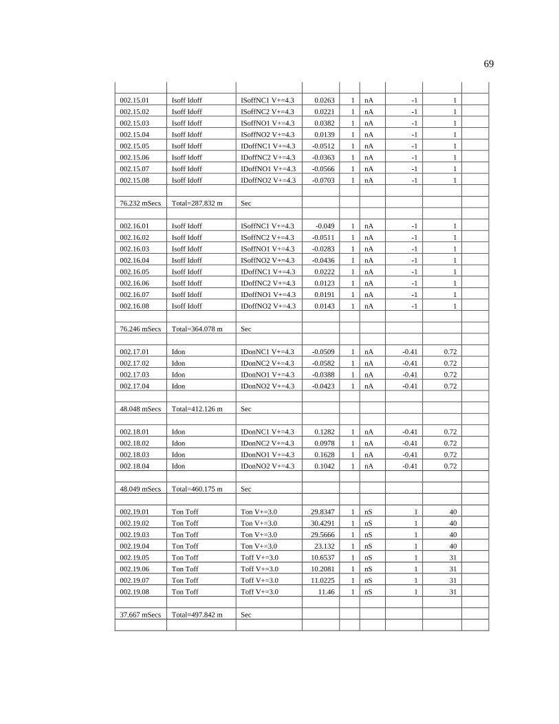
69
002.15.01 Isoff Idoff ISoffNC1 V+=4.3 0.0263 1 nA -1 1
002.15.02 Isoff Idoff ISoffNC2 V+=4.3 0.0221 1 nA -1 1
002.15.03 Isoff Idoff ISoffNO1 V+=4.3 0.0382 1 nA -1 1
002.15.04 Isoff Idoff ISoffNO2 V+=4.3 0.0139 1 nA -1 1
002.15.05 Isoff Idoff IDoffNC1 V+=4.3 -0.0512 1 nA -1 1
002.15.06 Isoff Idoff IDoffNC2 V+=4.3 -0.0363 1 nA -1 1
002.15.07 Isoff Idoff IDoffNO1 V+=4.3 -0.0566 1 nA -1 1
002.15.08 Isoff Idoff IDoffNO2 V+=4.3 -0.0703 1 nA -1 1
76.232 mSecs Total=287.832 m Sec
002.16.01 Isoff Idoff ISoffNC1 V+=4.3 -0.049 1 nA -1 1
002.16.02 Isoff Idoff ISoffNC2 V+=4.3 -0.0511 1 nA -1 1
002.16.03 Isoff Idoff ISoffNO1 V+=4.3 -0.0283 1 nA -1 1
002.16.04 Isoff Idoff ISoffNO2 V+=4.3 -0.0436 1 nA -1 1
002.16.05 Isoff Idoff IDoffNC1 V+=4.3 0.0222 1 nA -1 1
002.16.06 Isoff Idoff IDoffNC2 V+=4.3 0.0123 1 nA -1 1
002.16.07 Isoff Idoff IDoffNO1 V+=4.3 0.0191 1 nA -1 1
002.16.08 Isoff Idoff IDoffNO2 V+=4.3 0.0143 1 nA -1 1
76.246 mSecs Total=364.078 m Sec
002.17.01 Idon IDonNC1 V+=4.3 -0.0509 1 nA -0.41 0.72
002.17.02 Idon IDonNC2 V+=4.3 -0.0582 1 nA -0.41 0.72
002.17.03 Idon IDonNO1 V+=4.3 -0.0388 1 nA -0.41 0.72
002.17.04 Idon IDonNO2 V+=4.3 -0.0423 1 nA -0.41 0.72
48.048 mSecs Total=412.126 m Sec
002.18.01 Idon IDonNC1 V+=4.3 0.1282 1 nA -0.41 0.72
002.18.02 Idon IDonNC2 V+=4.3 0.0978 1 nA -0.41 0.72
002.18.03 Idon IDonNO1 V+=4.3 0.1628 1 nA -0.41 0.72
002.18.04 Idon IDonNO2 V+=4.3 0.1042 1 nA -0.41 0.72
48.049 mSecs Total=460.175 m Sec
002.19.01 Ton Toff Ton V+=3.0 29.8347 1 nS 1 40
002.19.02 Ton Toff Ton V+=3.0 30.4291 1 nS 1 40
002.19.03 Ton Toff Ton V+=3.0 29.5666 1 nS 1 40
002.19.04 Ton Toff Ton V+=3.0 23.132 1 nS 1 40
002.19.05 Ton Toff Toff V+=3.0 10.6537 1 nS 1 31
002.19.06 Ton Toff Toff V+=3.0 10.2081 1 nS 1 31
002.19.07 Ton Toff Toff V+=3.0 11.0225 1 nS 1 31
002.19.08 Ton Toff Toff V+=3.0 11.46 1 nS 1 31
37.667 mSecs Total=497.842 m Sec
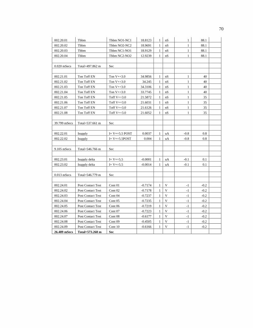
70
002.20.01 Tbbm Tbbm NO1-NC1 18.8123 1 nS 1 88.1
002.20.02 Tbbm Tbbm NO2-NC2 18.9691 1 nS 1 88.1
002.20.03 Tbbm Tbbm NC1-NO1 18.9129 1 nS 1 88.1
002.20.04 Tbbm Tbbm NC2-NO2 12.9239 1 nS 1 88.1
0.020 mSecs Total=497.862 m Sec
002.21.01 Ton Toff EN Ton V+=3.0 34.9856 1 nS 1 40
002.21.02 Ton Toff EN Ton V+=3.0 34.245 1 nS 1 40
002.21.03 Ton Toff EN Ton V+=3.0 34.3106 1 nS 1 40
002.21.04 Ton Toff EN Ton V+=3.0 33.7745 1 nS 1 40
002.21.05 Ton Toff EN Toff V+=3.0 21.5872 1 nS 1 35
002.21.06 Ton Toff EN Toff V+=3.0 21.6031 1 nS 1 35
002.21.07 Ton Toff EN Toff V+=3.0 21.6126 1 nS 1 35
002.21.08 Ton Toff EN Toff V+=3.0 21.6052 1 nS 1 35
39.799 mSecs Total=537.661 m Sec
002.22.01 Isupply I+ V+=5.5 POST 0.0037 1 uA -0.8 0.8
002.22.02 Isupply I+ V+=5.5POST 0.004 1 uA -0.8 0.8
9.105 mSecs Total=546.766 m Sec
002.23.01 Isupply delta I+ V+=5.5 -0.0001 1 uA -0.1 0.1
002.23.02 Isupply delta I+ V+=5.5 -0.0014 1 uA -0.1 0.1
0.013 mSecs Total=546.779 m Sec
002.24.01 Post Contact Test Cont 01 -0.7174 1 V -1 -0.2
002.24.02 Post Contact Test Cont 02 -0.7178 1 V -1 -0.2
002.24.03 Post Contact Test Cont 04 -0.7237 1 V -1 -0.2
002.24.04 Post Contact Test Cont 05 -0.7235 1 V -1 -0.2
002.24.05 Post Contact Test Cont 06 -0.7219 1 V -1 -0.2
002.24.06 Post Contact Test Cont 07 -0.7223 1 V -1 -0.2
002.24.07 Post Contact Test Cont 08 -0.6177 1 V -1 -0.2
002.24.08 Post Contact Test Cont 09 -0.4505 1 V -1 -0.2
002.24.09 Post Contact Test Cont 10 -0.6166 1 V -1 -0.2
26.489 mSecs Total=573.268 m Sec
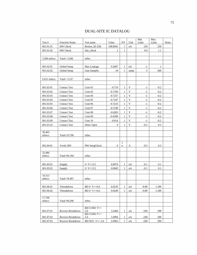
71
DUAL-SITE IC DATALOG
Test # Function Name Test name Value P/F Unit
Min
Limit
Max
Limit Notes
001.01.01 HW Check Resitor_ID 25K 198.8941 1 uA 150 250
001.01.02 HW Check Site_check 1 1 0.9 1.1
3.206 mSecs Total= 3.206 mSec
001.02.01 Global Setup Max Leakage 0.2087 1 nA -1 1
001.02.02 Global Setup Line Samples 18 1 samp 5 200
0.031 mSecs Total= 3.237 mSec
001.03.01 Contact Test Cont 01 -0.719 1 V -1 -0.2
001.03.02 Contact Test Cont 02 -0.7196 1 V -1 -0.2
001.03.03 Contact Test Cont 04 -0.7257 1 V -1 -0.2
001.03.04 Contact Test Cont 05 -0.7247 1 V -1 -0.2
001.03.05 Contact Test Cont 06 -0.7233 1 V -1 -0.2
001.03.06 Contact Test Cont 07 -0.7249 1 V -1 -0.2
001.03.07 Contact Test Cont 08 -0.6283 1 V -1 -0.2
001.03.08 Contact Test Cont 09 -0.4399 1 V -1 -0.2
001.03.09 Contact Test Cont 10 -0.614 1 V -1 -0.2
001.03.10 Contact Test Detec Open 0 1 V -0.5 0.5
30.463
mSecs Total=33.700 mSec
001.04.01 Verify HW HW IntegCheck 0
1
n A -0.5 0.5
32.484
mSecs Total=66.184 mSec
001.05.01 Isupply I+ V+=5.5 0.0074 1 uA -0.1 0.1
001.05.02 Isupply I+ V+=5.5 0.0045 1 uA -0.1 0.1
10.313
mSecs Total=76.497 mSec
001.06.01 Vbreakdown BD I+ V+=6.0 0.0235 1 uA -0.89 1.189
001.06.02 Vbreakdown BD I+ V+=6.0 0.0249 1 uA -0.89 1.189
17.709
mSecs Total=94.206 mSec
001.07.01 Reverse Breakdown
BD COM1 V+=
2.6 3.4466 1 uA -249 290
001.07.02 Reverse Breakdown
BD COM2 V+=
2.6 3.4994 1 uA -249 290
001.07.03 Reverse Breakdown BD NO1 V+= 2.6 2.6963 1 uA -249 290
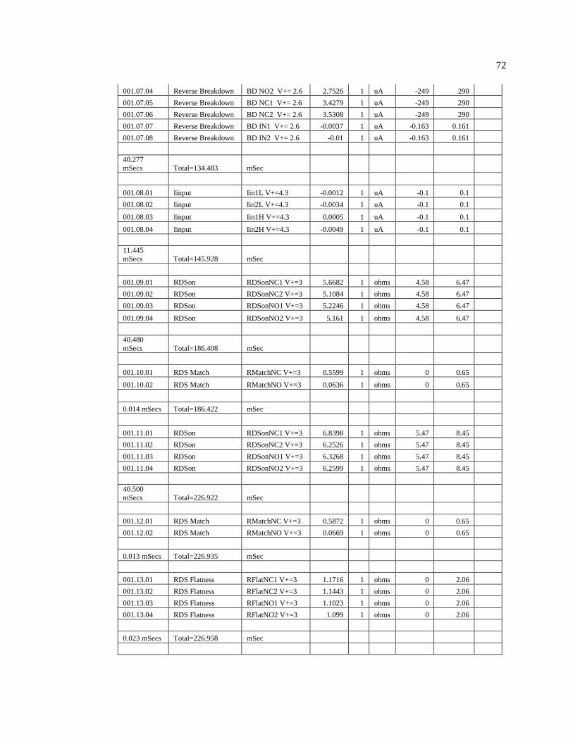
72
001.07.04 Reverse Breakdown BD NO2 V+= 2.6 2.7526 1 uA -249 290
001.07.05 Reverse Breakdown BD NC1 V+= 2.6 3.4279 1 uA -249 290
001.07.06 Reverse Breakdown BD NC2 V+= 2.6 3.5308 1 uA -249 290
001.07.07 Reverse Breakdown BD IN1 V+= 2.6 -0.0037 1 uA -0.163 0.161
001.07.08 Reverse Breakdown BD IN2 V+= 2.6 -0.01 1 uA -0.163 0.161
40.277 mSecs Total=134.483 mSec
001.08.01 Iinput Iin1L V+=4.3 -0.0012 1 uA -0.1 0.1
001.08.02 Iinput Iin2L V+=4.3 -0.0034 1 uA -0.1 0.1
001.08.03 Iinput Iin1H V+=4.3 0.0005 1 uA -0.1 0.1
001.08.04 Iinput Iin2H V+=4.3 -0.0049 1 uA -0.1 0.1
11.445
mSecs Total=145.928 mSec
001.09.01 RDSon RDSonNC1 V+=3 5.6682 1 ohms 4.58 6.47
001.09.02 RDSon RDSonNC2 V+=3 5.1084 1 ohms 4.58 6.47
001.09.03 RDSon RDSonNO1 V+=3 5.2246 1 ohms 4.58 6.47
001.09.04 RDSon RDSonNO2 V+=3 5.161 1 ohms 4.58 6.47
40.480
mSecs Total=186.408 mSec
001.10.01 RDS Match RMatchNC V+=3 0.5599 1 ohms 0 0.65
001.10.02 RDS Match RMatchNO V+=3 0.0636 1 ohms 0 0.65
0.014 mSecs Total=186.422 mSec
001.11.01 RDSon RDSonNC1 V+=3 6.8398 1 ohms 5.47 8.45
001.11.02 RDSon RDSonNC2 V+=3 6.2526 1 ohms 5.47 8.45
001.11.03 RDSon RDSonNO1 V+=3 6.3268 1 ohms 5.47 8.45
001.11.04 RDSon RDSonNO2 V+=3 6.2599 1 ohms 5.47 8.45
40.500
mSecs Total=226.922 mSec
001.12.01 RDS Match RMatchNC V+=3 0.5872 1 ohms 0 0.65
001.12.02 RDS Match RMatchNO V+=3 0.0669 1 ohms 0 0.65
0.013 mSecs Total=226.935 mSec
001.13.01 RDS Flatness RFlatNC1 V+=3 1.1716 1 ohms 0 2.06
001.13.02 RDS Flatness RFlatNC2 V+=3 1.1443 1 ohms 0 2.06
001.13.03 RDS Flatness RFlatNO1 V+=3 1.1023 1 ohms 0 2.06
001.13.04 RDS Flatness RFlatNO2 V+=3 1.099 1 ohms 0 2.06
0.023 mSecs Total=226.958 mSec
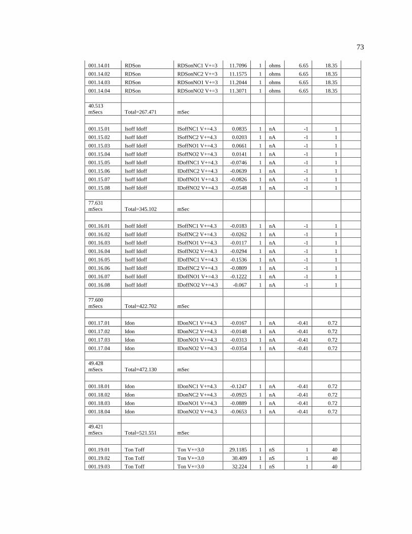
73
001.14.01 RDSon RDSonNC1 V+=3 11.7096 1 ohms 6.65 18.35
001.14.02 RDSon RDSonNC2 V+=3 11.1575 1 ohms 6.65 18.35
001.14.03 RDSon RDSonNO1 V+=3 11.2044 1 ohms 6.65 18.35
001.14.04 RDSon RDSonNO2 V+=3 11.3071 1 ohms 6.65 18.35
40.513
mSecs Total=267.471 mSec
001.15.01 Isoff Idoff ISoffNC1 V+=4.3 0.0835 1 nA -1 1
001.15.02 Isoff Idoff ISoffNC2 V+=4.3 0.0203 1 nA -1 1
001.15.03 Isoff Idoff ISoffNO1 V+=4.3 0.0661 1 nA -1 1
001.15.04 Isoff Idoff ISoffNO2 V+=4.3 0.0141 1 nA -1 1
001.15.05 Isoff Idoff IDoffNC1 V+=4.3 -0.0746 1 nA -1 1
001.15.06 Isoff Idoff IDoffNC2 V+=4.3 -0.0639 1 nA -1 1
001.15.07 Isoff Idoff IDoffNO1 V+=4.3 -0.0826 1 nA -1 1
001.15.08 Isoff Idoff IDoffNO2 V+=4.3 -0.0548 1 nA -1 1
77.631
mSecs Total=345.102 mSec
001.16.01 Isoff Idoff ISoffNC1 V+=4.3 -0.0183 1 nA -1 1
001.16.02 Isoff Idoff ISoffNC2 V+=4.3 -0.0262 1 nA -1 1
001.16.03 Isoff Idoff ISoffNO1 V+=4.3 -0.0117 1 nA -1 1
001.16.04 Isoff Idoff ISoffNO2 V+=4.3 -0.0294 1 nA -1 1
001.16.05 Isoff Idoff IDoffNC1 V+=4.3 -0.1536 1 nA -1 1
001.16.06 Isoff Idoff IDoffNC2 V+=4.3 -0.0809 1 nA -1 1
001.16.07 Isoff Idoff IDoffNO1 V+=4.3 -0.1222 1 nA -1 1
001.16.08 Isoff Idoff IDoffNO2 V+=4.3 -0.067 1 nA -1 1
77.600
mSecs Total=422.702 mSec
001.17.01 Idon IDonNC1 V+=4.3 -0.0167 1 nA -0.41 0.72
001.17.02 Idon IDonNC2 V+=4.3 -0.0148 1 nA -0.41 0.72
001.17.03 Idon IDonNO1 V+=4.3 -0.0313 1 nA -0.41 0.72
001.17.04 Idon IDonNO2 V+=4.3 -0.0354 1 nA -0.41 0.72
49.428
mSecs Total=472.130 mSec
001.18.01 Idon IDonNC1 V+=4.3 -0.1247 1 nA -0.41 0.72
001.18.02 Idon IDonNC2 V+=4.3 -0.0925 1 nA -0.41 0.72
001.18.03 Idon IDonNO1 V+=4.3 -0.0889 1 nA -0.41 0.72
001.18.04 Idon IDonNO2 V+=4.3 -0.0653 1 nA -0.41 0.72
49.421
mSecs Total=521.551 mSec
001.19.01 Ton Toff Ton V+=3.0 29.1185 1 nS 1 40
001.19.02 Ton Toff Ton V+=3.0 30.409 1 nS 1 40
001.19.03 Ton Toff Ton V+=3.0 32.224 1 nS 1 40
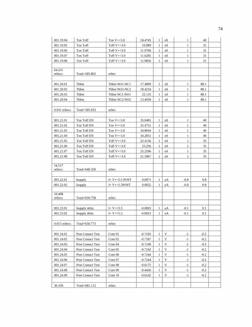
74
001.19.04 Ton Toff Ton V+=3.0 24.4745 1 nS 1 40
001.19.05 Ton Toff Toff V+=3.0 10.089 1 nS 1 31
001.19.06 Ton Toff Toff V+=3.0 11.0706 1 nS 1 31
001.19.07 Ton Toff Toff V+=3.0 11.6285 1 nS 1 31
001.19.08 Ton Toff Toff V+=3.0 11.9856 1 nS 1 31
64.251
mSecs Total=585.802 mSec
001.20.01 Tbbm Tbbm NO1-NC1 17.4899 1 nS 1 88.1
001.20.02 Tbbm Tbbm NO2-NC2 18.4234 1 nS 1 88.1
001.20.03 Tbbm Tbbm NC1-NO1 22.135 1 nS 1 88.1
001.20.04 Tbbm Tbbm NC2-NO2 13.4039 1 nS 1 88.1
0.031 mSecs Total=585.833 mSec
001.21.01 Ton Toff EN Ton V+=3.0 35.0481 1 nS 1 40
001.21.02 Ton Toff EN Ton V+=3.0 35.4751 1 nS 1 40
001.21.03 Ton Toff EN Ton V+=3.0 34.8044 1 nS 1 40
001.21.04 Ton Toff EN Ton V+=3.0 34.2831 1 nS 1 40
001.21.05 Ton Toff EN Toff V+=3.0 22.4136 1 nS 1 35
001.21.06 Ton Toff EN Toff V+=3.0 23.256 1 nS 1 35
001.21.07 Ton Toff EN Toff V+=3.0 25.2596 1 nS 1 35
001.21.08 Ton Toff EN Toff V+=3.0 21.5967 1 nS 1 35
54.517
mSecs Total=640.350 mSec
001.22.01 Isupply I+ V+=5.5 POST 0.0071 1 uA -0.8 0.8
001.22.02 Isupply I+ V+=5.5POST 0.0022 1 uA -0.8 0.8
10.408
mSecs Total=650.758 mSec
001.23.01 Isupply delta I+ V+=5.5 -0.0003 1 uA -0.1 0.1
001.23.02 Isupply delta I+ V+=5.5 -0.0023 1 uA -0.1 0.1
0.015 mSecs Total=650.773 mSec
001.24.01 Post Contact Test Cont 01 -0.7183 1 V -1 -0.2
001.24.02 Post Contact Test Cont 02 -0.7187 1 V -1 -0.2
001.24.03 Post Contact Test Cont 04 -0.7249 1 V -1 -0.2
001.24.04 Post Contact Test Cont 05 -0.7242 1 V -1 -0.2
001.24.05 Post Contact Test Cont 06 -0.7244 1 V -1 -0.2
001.24.06 Post Contact Test Cont 07 -0.7244 1 V -1 -0.2
001.24.07 Post Contact Test Cont 08 -0.6175 1 V -1 -0.2
001.24.08 Post Contact Test Cont 09 -0.4426 1 V -1 -0.2
001.24.09 Post Contact Test Cont 10 -0.6142 1 V -1 -0.2
30.339 Total=681.112 mSec
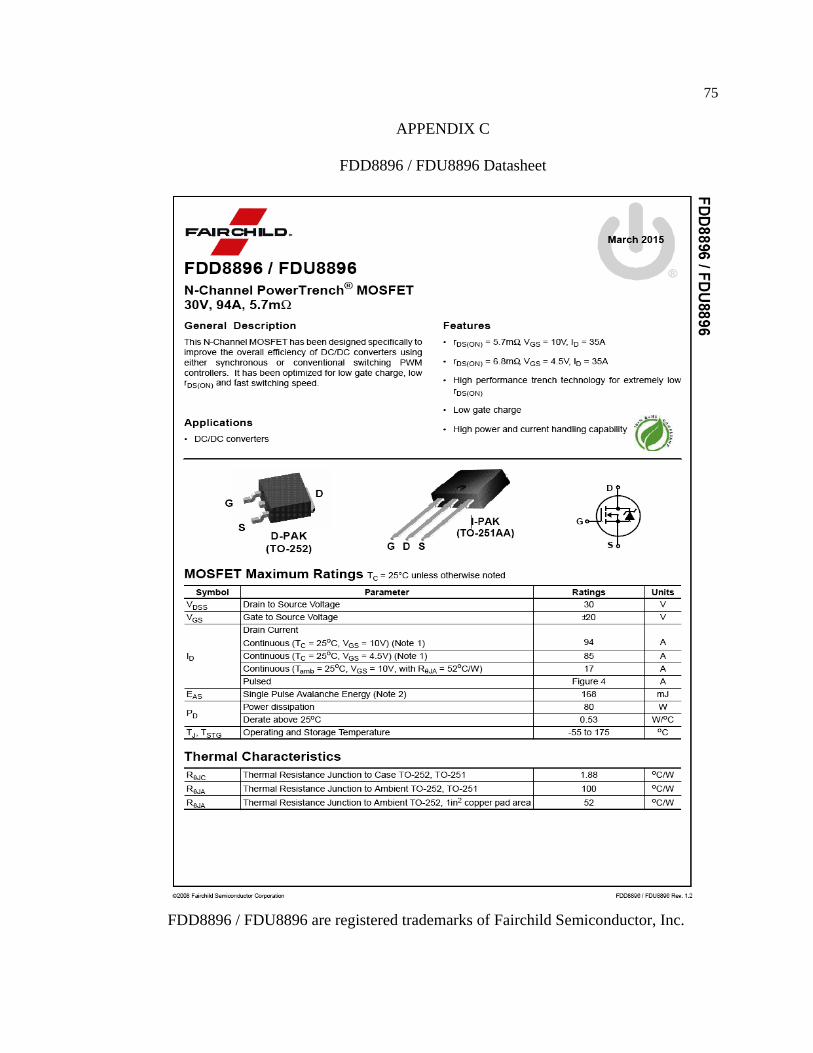
75
APPENDIX C
FDD8896 / FDU8896 Datasheet
FDD8896 / FDU8896 are registered trademarks of Fairchild Semiconductor, Inc.
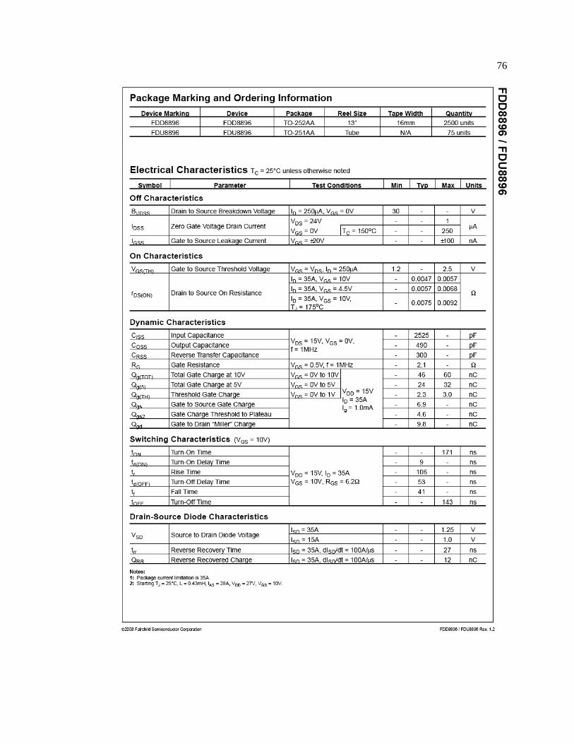
76
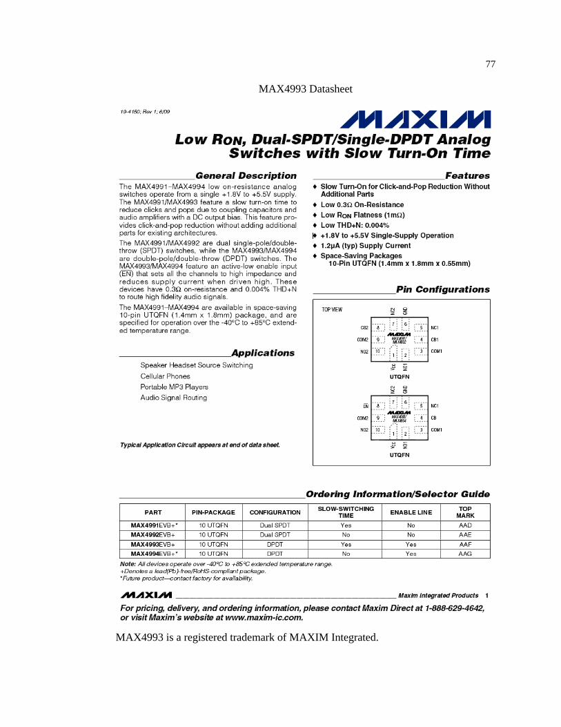
77
MAX4993 Datasheet
MAX4993 is a registered trademark of MAXIM Integrated.
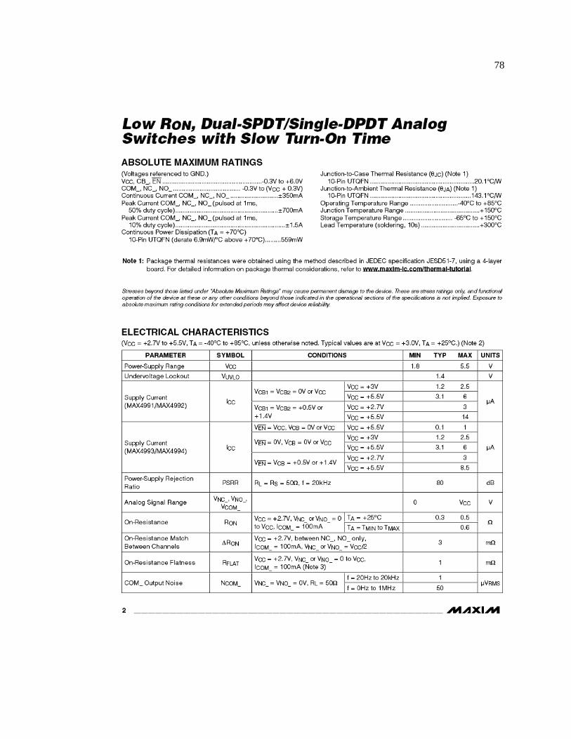
78
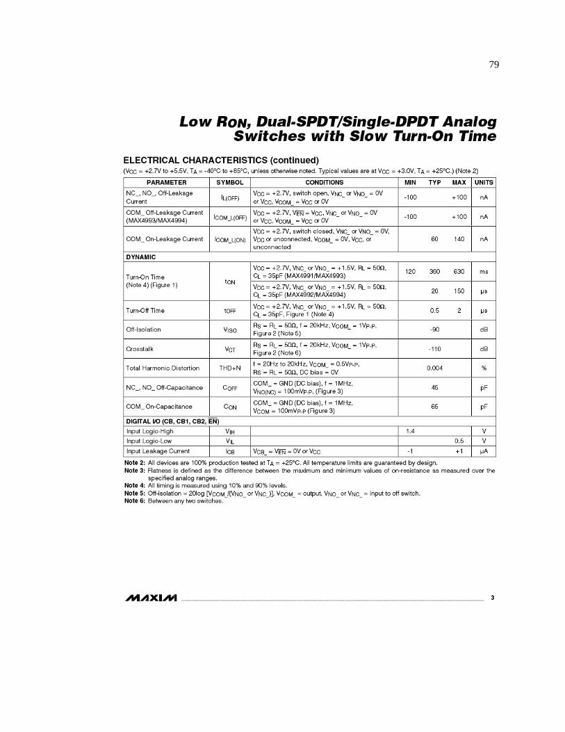
79
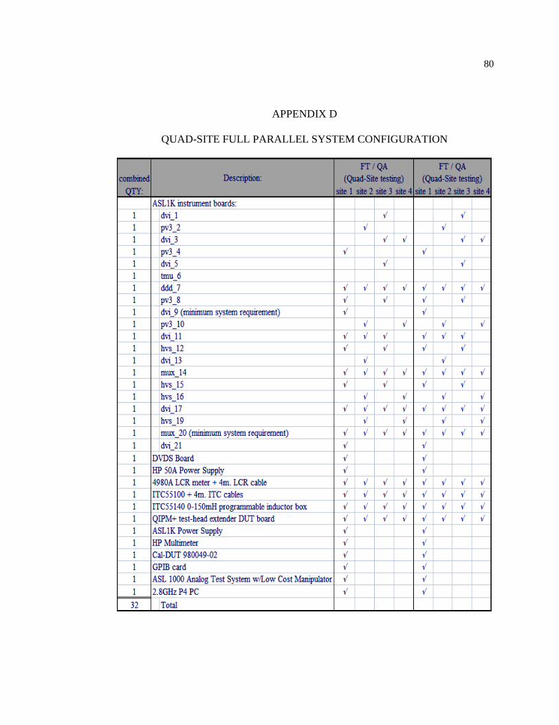
80
APPENDIX D
QUAD-SITE FULL PARALLEL SYSTEM CONFIGURATION
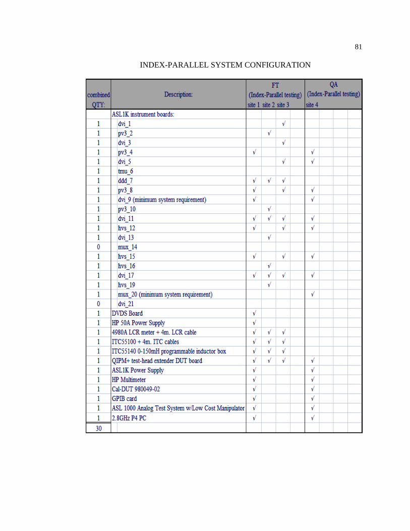
81
INDEX-PARALLEL SYSTEM CONFIGURATION
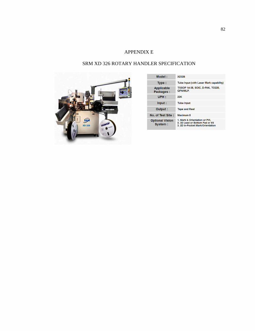
82
APPENDIX E
SRM XD 326 ROTARY HANDLER SPECIFICATION