Page | 1

Leverage1

In this chapter, we examine the impact of leverage on returns. We also explore the

concept of optimal leverage, and the Kelly criterion.

What is Leverage? In investing, leverage is the use of borrowed funds or derivatives to create returns in excess of what

could be generated through direct investment in an underlying asset. Leverage is often used by trading

desks and hedge funds in an attempt to increase returns on capital. In recent years asset managers have

even introduced leveraged exchange traded funds (ETFs) for retail investors.

In traditional asset management, given $100 of capital, a portfolio manager would buy $100 of

stocks, bond or other fundamental financial instruments. A portfolio manager that wished to use

leverage, by contrast, would borrow funds in order to buy additional assets. For example, a portfolio

manager with $100 of capital could borrow $200, and then purchase $300 of assets. In this case we

would say that the portfolio is levered three to one; that is for every $1 of capital the portfolio manager

has purchased $3 of assets.

In addition to borrowing, portfolio managers can also use derivatives to enhance returns. This

type of leverage can be referred to as implied or indirect leverage, as opposed to implicit or direct

leverage using borrowed funds. Take for example an equity call option with a price, P, of $10, and a

delta of 40%, where the underlying stock price, U, is $100. For a small move in the underlying, dU, the

change in price of the option, dP, will be approximated by:

Equation 1

where RU is the return on the underlying. Even though the option only costs $10, for small changes in

the underlying equity, the profit or loss is approximately $40 times the return of the underlying. Owning

$10 of the option is similar to owning $40 of the underlying equity. Of course the option is susceptible to

time decay, and changes in implied volatility, but, for small changes in the underlying, it’s as if we own

$40 of the equity. We can express this more formally by defining the leverage for an option, L, as:

1 This chapter is part of a series of chapters by Michael B. Miller, which can be found at www.risk256.com. Please

do not reproduce without permission. To request permission, or to provide feedback, you can contact the author, mike@risk256.com. This version of the chapter was last updated February 6, 2012.

Page | 2

Equation 2

In our current example, the leverage ratio is 4, (40% × $100) / $10 = 4.

Impact on Returns (One Period) The immediate impact of leverage on returns is easy to calculate. Assume that we can borrow funds at

the risk-free rate, Rrf, and that we use these funds to achieve a leverage ratio of L. Given the return on

an underlying asset, R, the return of the leveraged portfolio, RL, will be:

Equation 3

Here (L−1)Rrf represents the cost of borrowed funds. For an unlevered portfolio, L=1, we do not have to

borrow any funds. If we want to apply 3x leverage, L=3, then we need to borrow two times our initial

capital (e.g. $100 of capital plus $200 of borrowed funds). If L=0, rather than investing we are lending

our capital out at the risk-free rate, which results in a return of Rrf.

Be careful: it is a common mistake to assume that regular returns increase in proportion to the

leverage ratio. If the leverage used is modest, and the risk-free rate is close to zero, this may be a good

approximation, but it is only that, an approximation. When leverage is higher, or the risk-free rate is not

close to zero, this approximation can lead to significant approximation error.

Sample Problem

Question:

Archimedes Fund Group manages two portfolios. One portfolio is unlevered the other is levered

five times. Over two days, the unlevered fund returns +2.50% and −2.00%. Assume the daily cost

of borrowing is 0.01%. What were the returns for the levered fund?

Answer:

The return of the levered fund on the first day is 12.46%, and on the second day −10.04%.

Day 1:

Day 2:

Page | 3

We can simplify Equation 3 further by defining the excess return as then return on a portfolio or

asset minus the risk-free rate. Using a tilde to denote an excess return, and rearranging terms, we have:

Equation 4

Assuming we can borrow at the risk-free rate, excess returns do increase in direct proportion to our

leverage ratio. If a portfolio is levered three to one, then the excess return of the levered portfolio will

be exactly three times that of the unlevered portfolio.

One of the most popular measures of risk adjusted performance is the Sharpe ratio, named after

the Nobel Prize winning economist William Sharpe. The Sharpe ratio, S, is defined as a portfolio’s excess

return, divided by the standard deviation of its excess return.

Equation 5

For a leveraged portfolio, the standard deviation of the excess return is also directly

proportional to the leverage. For a leverage portfolio, then, the Sharpe ratio is:

Equation 6

The Sharpe ratio of a levered portfolio and the corresponding unlevered portfolio are equal. In other

words, the Sharpe ratio is invariant to leverage. Increasing leverage can increase returns, but it will also

increase risk. As long as we can borrow at the risk-free rate, the ratio of excess returns to their volatility

will not change.

In the preceding discussion, we have assumed that the portfolio manager can borrow at the risk-

free rate. Large financial institution can often borrow at very close to the risk-free rate. If borrowing

costs are greater than the risk-free rate then excess returns will increase more slowly, and the Sharpe

ratio will decrease as leverage increases.

Sample Problem

Question:

An asset manager manages two funds, MonoFund and TriFund. TriFund is exactly like MonoFund

except that it is three times levered. Over the most recent period, the measured Sharpe ratio of

Page | 4

MonoFund was 1.2, with a standard deviation of excess returns equal to 10%. What was the

return of MonFund during this period? For TriFund? Assume a risk-free rate of 2%, and that

TriFund can borrow at this rate.

Answer:

The return for MonoFund was 14%. The return for TriFund was 38%.

To find the return for MonoFund, we start by rearrange Equation 5 as follows:

For MonoFund the return is then 14%:

Because TriFund is just a leveraged version of MonoFund, and because it can borrow at the risk-

free rate, it will also have a Sharpe ratio of 1.2. The standard deviation of excess returns for

TriFund on the other hand will be three times as great, or 30%, 3 × 10% = 30%. Using the same

equation as before we obtain our final result:

Note that while the excess return of TriFund is three times that of MonoFund, the simple return

for TriFund, 38%, is less than three times as great as the simple return of MonoFund, 14%.

Risk and Bankruptcy Many risk statistics increase in proportion to leverage. Net exposure, gross exposure, standard

deviation and Value at Risk increase in direct proportion to leverage. Unexpected losses, the loss in

excess of the expected return, also increase in direct proportion to the leverage ratio. The probability

that a given loss occurs, on the other hand, will most likely not be proportional to the amount of

leverage used. In fact, the probability of a given loss occurring can increase dramatically with only a

small amount of leverage.

As an example, suppose that excess returns are normally distributed, and the standard deviation

of returns for an unlevered portfolio is 8%. What is the probability that the portfolio incurs an

unexpected loss of more than 24%? This would be a negative three standard deviation event, with a 1 in

741 chance of occurring. What if the portfolio were levered three times? Now the 24% loss is merely a

one standard deviation event with a 1 in 6 chance of occurring. In this example, leverage only increased

three times, but the likelihood of a 24% unexpected loss increased 118 times.

Page | 5

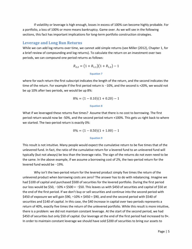
If volatility or leverage is high enough, losses in excess of 100% can become highly probable. For

a portfolio, a loss of 100% or more means bankruptcy. Game over. As we will see in the following

sections, this fact has important implications for long-term portfolio construction strategies.

Leverage and Long Run Returns While we can add log returns over time, we cannot add simple returns (see Miller (2012), Chapter 1, for

a brief review of compounding and log returns). To calculate the return on an investment over two

periods, we can compound one period returns as follows:

Equation 7

where for each return the first subscript indicates the length of the return, and the second indicates the

time of the return. For example if the first period return is −10%, and the second is +20%, we would not

be up 10% after two periods, we would be up 8%:

Equation 8

What if we leveraged these returns five times? Assume that there is no cost to borrowing. The first

period return would now be -50%, and the second period return +100%. This gets us right back to where

we started. The two-period return is exactly 0%:

Equation 9

This result is not intuitive. Many people would expect the cumulative return to be five times that of the

unlevered fund. In fact, the ratio of the cumulative return for a levered fund to an unlevered fund will

typically (but not always) be less than the leverage ratio. The sign of the returns do not even need to be

the same. In the above example, if we assume a borrowing cost of 2%, the two-period return for the

levered fund would be −19%.

Why isn’t the two-period return for the levered product simply five times the return of the

unlevered product when borrowing costs are zero? The answer has to do with rebalancing. Imagine we

had $100 of capital and purchased $500 of securities for the levered portfolio. During the first period

our loss would be $50, −10% × $500 = −$50. This leaves us with $450 of securities and capital of $50 at

the end of the first period. If we don’t buy or sell securities and continue into the second period with

$450 of exposure we will gain $90, +10% × $450 = $90, and end the second period with $540 of

securities and $140 of capital. In this case, the $40 increase in capital over two periods represents a

return of 40%, exactly five times the return of the unlevered portfolio. While this result is more intuitive,

there is a problem: we did not maintain constant leverage. At the start of the second period, we had

$450 of securities but only $50 of capital. Our leverage at the end of the first period had increased to 9×.

In order to maintain constant leverage we should have sold $200 of securities to bring our assets to

Page | 6

$250. With the rebalanced portfolio we would only have made $50 in the second period, bringing the

value of our securities up to $300, and bringing our capital back to $100. This is consistent with our

earlier result, a two-period return of 0%. Rebalancing is the key to understanding the impact of constant

leverage over multiple periods.

To maintain constant leverage, requires us to sell following negative returns and to buy

following positive returns. For fundamental investors this is tantamount to sell low and buy high, the

exact opposite of what a fundamental investor would do. While this might seem strange, this is what is

required to maintain constant leverage.

The advantage of constant leverage is that it acts to moderate risk levels. As before, imagine we

start with $100 of capital, lever five times and that our securities have a return of −10% in the first

period. At the end of the first period we have $50 of capital and $450 of assets. Now imagine that we

don’t rebalance the portfolio and that instead of a +20% return, the second period return is −12%. In the

second period our loss is $54, which completely wipes out our capital (and possibly leaves us $4 in debt).

If we had rebalanced, the loss would have been bad, −$30, but we would not have gone bankrupt.

Exposing yourself to higher leverage by failing to rebalance can be extremely risky.

For an individual investor, reducing leverage after a negative return should moderate risk.

Unfortunately, this strategy, if it is widespread, can be destabilizing for the market as a whole. If a large

negative returns forces widespread selling, prices will tend to fall further, which could lead to additional

selling, and on and on. Perversely if everybody tries to decrease their risk at the same time by

deleverage, they can end up increasing risk overall.

Optimization Increasing leverage will increase expected returns, but too much leverage can lead to large

losses and even bankruptcy. So is there an optimal amount of leverage? The question is deceptively

simple. The question has occupied some of finances best minds, and is closely related to advanced

problems in economics and information theory.

The problem of optimal leverage is somewhat analogous to the Saint Petersburg paradox2. In

the Saint Petersburg paradox you are offered a bet with an infinite expected payout. In theory you

should be willing to pay an infinite amount of money for this infinite expected payout. The only problem

is that the probability of large payouts is extremely small, and most of the time the games ends with

only a modest payout. If you pay a large amount to play this game, most of the time you will end up

losing money. Using excessive leverage in financial markets is similar. In theory you can make a lot of

money, but the probability is very small, and the most likely scenario is a large loss.

To start, let’s revisit our simple example where we have a −10% return followed by a +20%

return. At one extreme, if we use zero leverage, our return in both periods ends up being the risk-free

2 For a brief overview of the Saint Petersburg paradox, see the appendix.

Page | 7

rate. At the other extreme, if our leverage ratio is 10× or greater, we will end up bankrupt after the first

period, even if borrowing costs are zero. The graph below shows the cumulative return as a function of

leverage, assuming a 2% borrowing cost. In this case, the optimal leverage is approximately 1.42×, which

corresponds to a cumulative return of 8.38%. This is slightly better than the unlevered return (leverage

ratio equals one) of 8.00%. A leverage ratio slightly over 3× leads to negative returns, and a leverage

ratio of 8.5× or greater leads to bankruptcy.

Figure 1: Cumulative Returns as a Function of Leverage

Excessive leverage can lead can have a significantly negative impact on long-term performance

even if the leverage does not lead to bankruptcy. In the preceding example, a leverage ratio of 6.5× does

not lead to bankruptcy in the first period, but it leaves us with so little going into the second round that

it is hard to recover. With 6.5× leverage, the first period return is −76%. Even though the second period

return is a whopping +119%, the leaves two period return is only −47%.

In the preceding example finding the optimal amount of leverage was relatively easy because

we knew what the returns were going to be. What if future returns are unknown, but we do know the

distribution of future returns? The basic idea is the same as before: we want to magnify positive returns

as much as possible, while avoiding large negative returns. As simple as this sounds, it was not until the

1950s that a formal solution to the problem of optimal leverage was finally proposed.

-100%

-80%

-60%

-40%

-20%

0%

20%

0 1 2 3 4 5 6 7 8 9 10

Cu

mu

lati

ve R

etu

rn

Leverage Ratio

Page | 8

In 1956, John Kelly, Jr, a scientist at Bell Labs published a paper outlining what seemed to offer a

novel approach to the question of optimal leverage under uncertainty. Rather than trying to minimize

the probability of bankruptcy or maximize the expected return, Kelly tried to maximize the expected

long-term log return. This approach was strongly rooted in information theory. In fact, in the first page

of his paper, he cites the work of his Bell Lab coworker, Claude Shannon, the father of information

theory.

Kelly’s original paper dealt with simple discrete bets, but it is relatively simple to extend the

basic approach to continuous distributions. As before, we define the excess return at time t as , and

the leverage ratio as L. The cumulative excess return over n periods, , can then be found as follows:

Equation 10

Taking the log of both sides, and using our convention of lowercase letters to denote log returns, we

have:

Equation 11

For the right-hand side of the equation, we cannot simply move the leverage term outside the

logarithm; that is . We can however calculate the second order Taylor expansion for

this term as follows (see Miller (2012), Appendix, for an overview of Taylor expansions):

Equation 12

Taking the expectations of this equation and denoting the mean and standard deviation of the excess

return by µ and σ, respectively, we have:

Equation 13

Substituting back into our equation for the cumulative return, we have:

Equation 14

Page | 9

Finally we define the average excess log return, , as divided by the number of periods, n. This gives

us:

Equation 15

It was a long time in coming but it is this average expected excess log return, , that Kelly would

have us maximize. To find the optimal value of L, L*, we take the derivative with respect to L, and set

this equal to zero:

Equation 16

We note that the second derivative, , is unambiguously negative, so our solution is indeed a

maximum.

If µ is small relative to σ then we can approximate L* as µ/σ2. For i.i.d. returns µ becomes

increasingly small relative to σ as we increase the frequency of observations. If µ and σ are measured

using daily observations µ/σ2 will generally be a valid approximation.

For i.i.d. returns the approximation µ/σ2 is frequency invariant, both µ and σ2 are linear in time,

and the ratio will be the same if we measure µ and σ2 using daily, monthly or annual data. This is not

true for the full formula in Equation 16. It is not difficult to show that for i.i.d. returns L* decreases as

the frequency of our observations decreases. In other words, if we rebalance less frequently we should

use less leverage. Remember from the previous section that to maintain constant leverage, we needed

to reduce the size of our portfolio after a negative return, which reduced risk. If we fail to rebalance or

rebalance less often large and potentially devastating drawdowns become more likely. This is why the

optimal leverage ratio decreases as the frequency of rebalancing decreases. As a rule, you should

ensure that the frequency with which you are rebalancing matches the frequency with which you are

measuring the µ and σ2.

Sample Problem

Question:

For our two-period example where we have a −10% return followed by a +20% return, and

borrowing costs are 2%, calculate the optimal leverage ratio using Equation 16. For this problem,

because all of the returns are known, use the population mean and variance.

Page | 10

Answer:

The excess returns in the first and second periods are −12% and +18%, respectively. The mean

excess return is then 3%:

The population variance is 2.29%:

Our final answer is then a leverage ratio of 1.26:

The final answer is close to, but not exactly the same as, the actual optimal leverage ratio of 1.42.

The difference stems from our use of the Taylor approximation in Equation 13.

We can substitute the optimal leverage ratio back into our equation for the average excess log

return to get the optimal expected average excess log return:

Equation 17

In the last step, we discover that the optimal excess return can be expressed solely in terms of the

Sharpe ratio. This result is reassuring. If two securities have the same Sharpe ratio then they will also

have the same optimal excess return. As long as we can borrow at the risk-free rate, the optimal

performance of our portfolio is no longer constrained by the excepted excess return of our securities;

rather, the performance is determined by the Sharpe ratio, the risk-adjusted excess return. The

following chart shows the optimal excess return as a function of the Sharpe ratio.

Page | 11

Figure 2: Expected Optimal Return as a Function of the Sharpe Ratio

So how do we these results work in practice? The following graph shows the hypothetical

returns of a leveraged investment in the Standard and Poor’s 500 Index (S&P 500) from 1989 through

2011. The portfolio is rebalanced daily, and the cost of borrowing is assumed to be the risk-free rate.

0%

10%

20%

30%

40%

50%

60%

0 1 2 3

Op

tim

al E

xce

ss R

etu

rn

Sharpe

Page | 12

Figure 3: Leverage and S&P 500 Returns, 1989-2011

As can be seen, the annualized return increases with leverage until it reaches a maximum at 10.96%,

corresponding to a leverage of 1.97. Beyond this point more leverage detracts from long-term

performance, and beyond a leverage ratio of 4.3 realized returns are negative. If we use the sample

mean and standard deviation for the entire 23 year period, our formula for the optimal leverage ratio

returns 1.98. This is extremely close to the actual optimal leverage ratio, and the annualized return is

almost exactly the same, 10.960% versus 10.961%.

Suppose we had invested in the S&P 500 from 1989 through 2011 using a leverage ratio of 1.98,

how would we have done? The average annualized return would have been 10.96% versus 9.15% for an

unlevered investment. This doesn’t seem like a huge improvement, but this small difference adds up

over time. If we had started with $100 in 1989, our unlevered investment would have been worth $749

at the end of 2011, but our levered investment would have been worth $1,094. This is a 46%

improvement over the unlevered result. Not bad! Still, maintaining even this modest level of leverage

would have led to some rather large swings in the value of the portfolio. In 2008, rather than a loss of

37%, the levered portfolio would have sustained a loss of 66%.

The preceding historical analysis seems to suggest that beating the market in the long-run is

easy. Starting in 1989 all we needed to do was borrow some funds, invest in the S&P 500, rebalance

from time to time, kick back, and watch the money pour in. Sure there would have been some ups and

downs, but we could rest easy, confident in our long-term strategy. Of course, all of this assumes that

we would have known back in 1989 that the optimal leverage over the next 23 years would be 1.98 (or,

-8%

-6%

-4%

-2%

0%

2%

4%

6%

8%

10%

12%

0.0 0.5 1.0 1.5 2.0 2.5 3.0 3.5 4.0 4.5 5.0

An

nu

aliz

ed

Re

turn

Leverage

Page | 13

even better, 1.97). Unfortunately it is not so obvious that we would have been able to determine this

optimal leverage ratio back in 1989. Figure 4 shows the optimal leverage ratio calculated using the same

data set as before using a rolling 10 year window. Even though our window is fairly long, the optimal

ratio changes dramatically, starting at just over 7 in 1998, and eventually turning slightly negative in

2009. If we had invested using this rolling 10-year estimate, the results would not have been good. Over

13 years our average annual return would have been -26%. At the end of 13 years we would have lost

97% of our initial investment. Admittedly, this was a tough time to be invested in equity markets, but an

unlevered investment still would have made money over this period, with an annualized return of

2.26%, and a total return of 29%.

Figure 4: S&P 500 Optimal Leverage, Rolling 10-Year Window

Leverage is a powerful financial tool. A portfolio’s risk and performance can be meaningfully

altered by the application of even modest amounts of leverage. Over long periods of time small

amounts of leverage can greatly enhance returns, but leverage can also easily lead to ruin.

Problems 1. OctoFund maintains a leverage ratio of 8:1. Unlevered returns over three periods are 3.20%,

−5.00%, and 8.00%. The borrowing cost in each period is 0.20%. What are the returns for

OctoFund over these three periods?

2. Using the same information provided in problem 1, what was the cumulative return for

OctoFund and for the unlevered investment?

-2

-1

0

1

2

3

4

5

6

7

8

L*

Page | 14

3. The Sharpe ratio of a hedge fund is 2.0. The annualized standard deviation of the fund’s excess

returns is 3.20%. Assume a risk-free rate and borrowing cost of 3.00%. What is the expected

return of 2.5× leveraged version of this fund?

4. The expected annualized return of an index is 12.80%, with a standard deviation of 32.00%.

What is the optimal leverage ratio? Assume returns are i.i.d., daily rebalancing, and 256 business

days in a year.

Page | 15

Appendix

Saint Petersburg Paradox The Saint Petersburg paradox was famously described and explored in the eighteenth century by Daniel

and Nicolas Bernoulli. Nicolas is credited with one of the first known descriptions of the paradox, while

his cousin Daniel engaged in extensive formal analysis of the problem.

Imagined you are invited to bet on successive flips of a fair coin. On the initial flip if the coin

lands on heads you receive $2 and the game continues. For the second flip, the payout doubles and

heads results in an additional gain of $4. As long as the coin continues to land on heads, the game

continues with payouts doubling in each successive round. If at any time the coin lands on tails, though,

you receive nothing for that round and the game is terminated. For example, if the coin lands on heads

four time and then tails, you would win $30, $2 + $4 + $8 + $16 = $30.

The expected value of this game can be found as follows:

In each successive round the payout doubles but the probability is getting to that round is half as much.

Multiplying through, we have:

The expected value of each successive round is constant at $1, and, in theory, the expected value of the

game is infinite. The paradox is that even though the game has an infinite expected value, most people

would not pay anywhere near an infinite amount of money to play this game.

To be fair, there are some practical issues with the problem. The most obvious is that payouts

grow at an exponential rate. In the current set up, the payout would be just over one million dollars for

the twentieth coin flip. By the thirtieth coin flip, the incremental payout would be over one billion

dollars. Still if the person you are playing this game with has some very deep pockets, the infinite version

of this game is impractical. Even if we restrict ourselves to a finite version of this game, we are likely to

find participants unwilling to pay the expected value of the game. Daniel Bernoulli’s solution to the

paradox turns out to be applicable in either an infinite or finite version of the game. Bernoulli proposed

what modern economists would describe as decreasing marginal utility. This decreasing marginal utility

in turn leads to risk aversion.

For economist the ultimate value of goods and services is not their monetary value, but in the

satisfaction or utility that we receive from those goods and services. The utility that you receive from

goods or services is not perfectly correlated with their monetary value and depends on all sorts of

factors, including your tastes, when the consumption happens, and what else you are consuming. Most

importantly, for most people and for most items, the more you consume of something the less utility

you get from each additional unit that you consume. This is what economists refer to as decreasing

marginal utility. Pretend that your favorite thing in the world is ice cream sundaes, and that you are

Page | 16

currently eating zero sundaes per week. If somebody gives you one sundae you’ll be extremely happy. If

they offer you a second sundae you’ll be even happier, but probably not twice as happy. At some point

you’ll be eating sundaes for breakfast, lunch and dinner, at which point you might not even want an

additional sundae. Each marginal sundae provides less utility than the sundae before. The same is true

for cars, vacations, houses and even for money. A gift of one million dollars should make you happy, but

two million dollars will not make you twice as happy.

If people try to maximize expected utility instead of expected monetary value and there is

declining marginal utility then people will tend to be risk averse. Given the choice between a sure bet

and a risky proposition with the same expected value, a risk averse individual will prefer the sure bet.

Imagine a person with the following utility function for money:

Dollars Utility

$0 0

$100 100

$200 180

$300 140

Notice that utility continues to increase with the amount of money, but at a decreasing rate. The first

$100 leads to a utility of 100, but the second only increases utility by 80, and the third by 60. If this

person were offered $200 with certainty or a 50:50 chance at $100 or $300, they would choose $200

with certainty. Even though both options have the same expected monetary value, $200, they have

different expected utility. The expected utility of $200 with certainty is 180, while the utility of the 50:50

bet is only 120, 0.5 × 100 + 0.5 × 140 = 120.

For the Saint Petersburg paradox, imagine a finite version of our coin flipping game, which

terminates after 20 rounds. The expected monetary value of the game is $20, but the large potential

payouts in the final rounds don’t provide nearly as much utility relative to their monetary value. Most

people are risk averse and would only be willing to play this game if it cost less than $20. If a person’s

utility function is declining quickly enough then even the infinite game will only be worth a finite amount

of money. This was Bernoulli’s solution to the paradox.

In more recent years, economists have refined their models of how people evaluate utility.

These new models can explain a wide variety of observed behaviors. The basic idea, that utility and not

dollars is what matters, still holds, and offers the surest explanation of the Saint Petersburg paradox.

Page | 17

References Kelly, J. L., Jr. 1956. "A New Interpretation of Information Rate." Bell System Technical Journal 35: 917–

926.

Miller, Michael B. 2012. Mathematics and Statistics for Financial Risk Management. New York: John

Wiley & Sons.

Shannon, C. E. 1948. “A Mathematical Theory of Communication.” Bell System Technical Journal 27:

379–423 and 623–656.

Page | 18

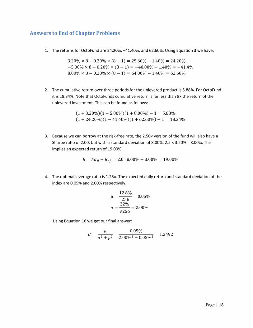
Answers to End of Chapter Problems

1. The returns for OctoFund are 24.20%, −41.40%, and 62.60%. Using Equation 3 we have:

2. The cumulative return over three periods for the unlevered product is 5.88%. For OctoFund

it is 18.34%. Note that OctoFunds cumulative return is far less than 8× the return of the

unlevered investment. This can be found as follows:

3. Because we can borrow at the risk-free rate, the 2.50× version of the fund will also have a

Sharpe ratio of 2.00, but with a standard deviation of 8.00%, 2.5 × 3.20% = 8.00%. This

implies an expected return of 19.00%.

4. The optimal leverage ratio is 1.25×. The expected daily return and standard deviation of the

index are 0.05% and 2.00% respectively.

Using Equation 16 we get our final answer: