Clemson UniversityTigerPrints

All Dissertations Dissertations

8-2014

Level stripping of genus 2 Siegel modular formsRodney KeatonClemson University, rkeaton@clemson.edu

Follow this and additional works at: https://tigerprints.clemson.edu/all_dissertations

Part of the Applied Mathematics Commons

This Dissertation is brought to you for free and open access by the Dissertations at TigerPrints. It has been accepted for inclusion in All Dissertations byan authorized administrator of TigerPrints. For more information, please contact kokeefe@clemson.edu.

Recommended CitationKeaton, Rodney, "Level stripping of genus 2 Siegel modular forms" (2014). All Dissertations. 1294.https://tigerprints.clemson.edu/all_dissertations/1294

Level stripping of genus 2 Siegel modular forms

A Dissertation

Presented to

the Graduate School of

Clemson University

In Partial Fulfillment

of the Requirements for the Degree

Doctor of Philosophy

Mathematical Sciences

by

Rodney Lewis Keaton

August 2014

Accepted by:

Associate Professor Jim Brown, Committee Chair

Professor Kevin James

Associate Professor Hui Xue

Assistant Professor Michael Burr

Abstract

In this dissertation we consider stripping primes from the level of genus 2 cus-

pidal Siegel eigenforms. Specifically, given an eigenform of level N`r which satisfies

certain mild conditions, where ` - N is a prime, we construct an eigenform of level N

which is congruent to our original form. To obtain our results, we use explicit con-

structions of Eisenstein series and theta functions to adapt ideas from a level stripping

result on elliptic modular forms. Furthermore, we give applications of this result to

Galois representations and provide evidence for an analog of Serre’s conjecture in the

genus 2 case.

ii

For Anna and Evelyn

iii

Acknowledgments

First and foremost, I would like to express my utmost gratitude for my advisor

Jim Brown. Throughout my time as a graduate student, he has guided me with

patience and many words of encouragement. Without him, this dissertation would

not have been possible. I would also like to thank my committee members Hui Xue,

Kevin James, and Michael Burr for all of the helpful advice and insightful discussions

over the years.

My close friends Allison Gaines, Caitlin McMahon, Charles Gamble, Charles

and Erin McPillan, and James Johnson deserve special thanks for their constant

support. Furthermore, I appreciate the friendship and many helpful mathematical

discussions with my colleagues Chris and Christa Johnson, Dania Zantout, Patrick

Buckingham, and Rachel Grotheer.

I would also like to express my appreciation for my family. The love of my

brother, sister, parents, and grandparents has given me a firm foundation which I

have been able to rely upon my whole life.

Finally, my deepest thanks goes to my wonderful wife Anna. Her unwaiver-

ing belief in me has has been invaluable in weathering the many ups and downs of

graduate school.

iv

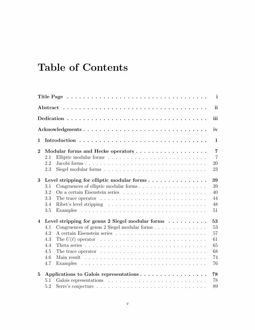
Table of Contents

Title Page . . . . . . . . . . . . . . . . . . . . . . . . . . . . . . . . . . . i

Abstract . . . . . . . . . . . . . . . . . . . . . . . . . . . . . . . . . . . . ii

Dedication . . . . . . . . . . . . . . . . . . . . . . . . . . . . . . . . . . . iii

Acknowledgments . . . . . . . . . . . . . . . . . . . . . . . . . . . . . . . iv

1 Introduction . . . . . . . . . . . . . . . . . . . . . . . . . . . . . . . . 1

2 Modular forms and Hecke operators . . . . . . . . . . . . . . . . . . 72.1 Elliptic modular forms . . . . . . . . . . . . . . . . . . . . . . . . . . 72.2 Jacobi forms . . . . . . . . . . . . . . . . . . . . . . . . . . . . . . . . 202.3 Siegel modular forms . . . . . . . . . . . . . . . . . . . . . . . . . . . 23

3 Level stripping for elliptic modular forms . . . . . . . . . . . . . . . 393.1 Congruences of elliptic modular forms . . . . . . . . . . . . . . . . . . 393.2 On a certain Eisenstein series . . . . . . . . . . . . . . . . . . . . . . 403.3 The trace operator . . . . . . . . . . . . . . . . . . . . . . . . . . . . 443.4 Ribet’s level stripping . . . . . . . . . . . . . . . . . . . . . . . . . . 483.5 Examples . . . . . . . . . . . . . . . . . . . . . . . . . . . . . . . . . 51

4 Level stripping for genus 2 Siegel modular forms . . . . . . . . . . 534.1 Congruences of genus 2 Siegel modular forms . . . . . . . . . . . . . . 534.2 A certain Eisenstein series . . . . . . . . . . . . . . . . . . . . . . . . 574.3 The U(`) operator . . . . . . . . . . . . . . . . . . . . . . . . . . . . 614.4 Theta series . . . . . . . . . . . . . . . . . . . . . . . . . . . . . . . . 654.5 The trace operator . . . . . . . . . . . . . . . . . . . . . . . . . . . . 684.6 Main result . . . . . . . . . . . . . . . . . . . . . . . . . . . . . . . . 744.7 Examples . . . . . . . . . . . . . . . . . . . . . . . . . . . . . . . . . 76

5 Applications to Galois representations . . . . . . . . . . . . . . . . . 785.1 Galois representations . . . . . . . . . . . . . . . . . . . . . . . . . . 785.2 Serre’s conjecture . . . . . . . . . . . . . . . . . . . . . . . . . . . . . 89

v

5.3 A Serre type conjecture in genus 2 . . . . . . . . . . . . . . . . . . . . 99

6 Future work . . . . . . . . . . . . . . . . . . . . . . . . . . . . . . . . 1066.1 Twisting of Siegel modular forms . . . . . . . . . . . . . . . . . . . . 1066.2 Level stripping for reducible Galois representations . . . . . . . . . . 1076.3 Level stripping for arbitrary genus . . . . . . . . . . . . . . . . . . . . 1086.4 Level stripping of automorphic representations . . . . . . . . . . . . . 109

Appendices . . . . . . . . . . . . . . . . . . . . . . . . . . . . . . . . . . . 111A Explicit action of Hecke operators in genus 2 . . . . . . . . . . . . . . 112B The Deligne-Serre lifting lemma . . . . . . . . . . . . . . . . . . . . . 119

Bibliography . . . . . . . . . . . . . . . . . . . . . . . . . . . . . . . . . . 125

vi

Chapter 1

Introduction

In modern number theory, a primary object of interest is the absolute Ga-

lois group of the rationals, i.e., GQ := Gal(Q/Q). As this group tends to be quite

unapproachable by any direct means, it is necessary to consider more sophisticated

techniques. For instance, throughout this dissertation we will be broadly interested

in using representation theory to extract information about GQ. In particular, we will

consider representations of GQ, called Galois representations, which arise from certain

automorphic forms. This method for studying GQ has become commonplace over the

past fifty to sixty years. In fact, all techniques of this type used to better understand

GQ can be fit into a much more general framework known as the Langland’s program,

which is one of the primary engines driving modern number theory.

For motivation, we consider the simplest case, i.e., the one dimensional com-

plex Galois representations. To be more precise, these are continuous homomorphisms

of the form

ρ : GQ → GL1(C).

A natural question to ask about these representations, and a question which we will

1

return to many times is, how many of these representations arise from automorphic

forms? We will not be overly concerned with making this question and the results

surrounding more precise in this setting, as it is well documented in the literature, but

we will consider its higher dimensional analogues in considerable depth in Chapter 5.

We begin by simply considering the basic properties of ρ. As a result of the

continuity condition, one can show that the image of ρ is finite (see Chapter 5). By

the Kronecker-Weber theorem, we have that the map ρ factors through the finite

Galois group Gal(Q(ζN)/Q), where N is some positive integer and ζN is a primitive

N th root of unity. As Gal(Q(ζN)/Q) is isomorphic to (Z/NZ)x, we see that ρ can be

viewed as an element of the dual group of (Z/NZ)x, i.e., ρ can be viewed a Dirichlet

character modulo N . As this process is reversible, we have a bijection between one

dimensional complex representations of GQ and Dirichlet characters.

In order to connect this classification of one dimensional complex representa-

tions of GQ with the theory of automorphic forms, we have the groundbreaking work

done in Tate’s thesis ([70]). Without saying too much, Tate’s thesis gives, among

other things, that there is a bijection between the set of all Hecke characters of finite

order and the set of all Dirichlet characters. In the one dimensional case, it is the

Hecke characters which play the role of the automorphic forms. While a detailed

explanation of what this means and the implications thereof would take us too far

afield, the interested reader is referred to Section 3.1 in [15] for an exposition of Tate’s

thesis and Section 2.1 in [29] for a particularly nice interpretation of Hecke characters

as automorphic forms. In summary, to answer the rough question given above, we

have that all one dimensional complex Galois representation arise from automorphic

forms.

As was mentioned previously, these one dimensional complex representations

always have finite image. As GQ is far from a finite group, it stands to reason that

2

we have lost considerable information by considering only these representations. As

will be discussed later, due to the continuity condition, there is a richer theory of one

dimensional Galois representations whose image is contained in the `-adic numbers or

a finite extension thereof, where ` is a rational prime. However, these one dimensional

`-adic representations can still only capture the Abelian structure of GQ, and hence

considerable information is still lost. In order to capture any non-Abelian structure

of GQ, we must consider higher dimensional Galois representations. The natural next

step is to consider two dimensional Galois representations.

There are several known constructions of these two dimensional Galois rep-

resentations. In particular, from the work of Deligne [20], we can construct a two

dimensional Galois representation from an elliptic Hecke eigenform whose image lies

in some `-adic number field. We will refer to such a Galois representation as modular.

In this case, the determinant and trace of the representation can be expressed in terms

of the Hecke eigenvalues. Unlike in the one dimensional setting, this construction of

Deligne falls far short of providing us with all two dimensional Galois representa-

tions. For example, if the determinant of the image of complex conjugation under

the representation is 1, then such a representation cannot arise from such a construc-

tion. While we know that we will not obtain all such representations, one can still

ask, which Galois representations do arise from elliptic Hecke eigenforms? Note, here

elliptic Hecke eigenforms are playing the role of the appropriate automorphic forms

just as the Hecke characters did in the previous discussion.

By moving to the two dimensional this question has already become much

harder to answer. In fact, at the writing of this dissertation, it is still an open problem

and an active area of research. However, considerable progress has been made on this

question, with far reaching consequences. The most notable example, perhaps, is the

proof of the Taniyama-Shimura conjecture, see [13], [72], and [83]. The content of

3

their proof being that they show that a certain large class of two dimensional Galois

representations, namely those arising from elliptic curves, are in fact modular. As

a direct application to classical number theory, the proof of this conjecture implies

Fermat’s last theorem.

As we have mentioned, general two dimensional Galois representations are

quite difficult to work with. In order to make things a bit easier to, we consider

two dimensional residual representations, i.e., two dimensional representations whose

image lies in the algebraic closure of some finite field. To this end, let K be a number

field with ν a prime lying over ` and let

ρ : Gal(Q/Q)→ GL2(OKν )

be a Galois representation, where Kν is the completion of K at ν. Let ρ denote

the residual representation of ρ obtained by composition with the map GL2(OKν )→

GL2(Fν), where Fν is the residue field of OK at ν. Then, it makes sense to ask the

analogous question, which two dimensional Galois representations of the form

ρ : Gal(Q/Q)→ GL2(Fν)

arise as the residual representation of a modular Galois representation?

By passing to the residual representation, this becomes an easier question. In

fact, by Serre’s conjecture (3.2.4?,[64]), which is now known to be a theorem ([43]), we

know precisely the conditions necessary for the semisimplification of ρ to be modular.

Furthermore, Serre’s refined conjecture (3.2.4?,[64]) tells us the precise character,

level, and weight of such an eigenform. Note, the equivalence of Serre’s conjecture

and Serre’s refined conjecture is known by the work of Coleman-Voloch [18], Gross

4

[30], Ribet [59], and others (see [22]). In the process of proving this equivalence, Ribet

presented the following result which we will be interested in extending.

Theorem 1. [60, Theorem 2.1]

Let ` ≥ 3 be a prime. Suppose that f is an eigenform of level N`r with r > 0 and

(N, `) = 1. Then, there exists an eigenform of level N whose eigenvalues away from

the level of f are congruent to the eigenvalues f modulo `.

In Chapter 3, we give a detailed proof of this result, as the techniques will be

quite similar to the proof of the main result of this dissertation.

In summary, we see that while we are not able to provide any answer to the

question regarding general two dimensional Galois representations, we do have quite

a satisfying theory of two dimensional residual representations. In this dissertation,

we will be interested in adapting some of this theory of two dimensional residual

representations to the four dimensional setting.

In order to transfer to the setting we will primarily be interested in, we let

ρ : Gal(Q/Q)→ GSp4(OKν )

be a Galois representation, where we are keeping the same notation as above. In this

setting there is a conjecture of Herzig and Tilouine which serves as an analogue to

Serre’s conjecture. In particular, this conjecture gives conditions on when the residual

representation of ρ should arise from a genus 2 Siegel eigenform, see Section 5.3 for

details. Given a conjecture of this form it is natural to want some type of refined

conjecture to make precise the character, level, and weight of such an eigenform. The

desired weight is discussed in detail in [33]. Concerning the level, a natural starting

place is Theorem 55, which is our analogue to Theorem 1 in the genus 2 setting.

5

Similar results have been obtained using an extension of Hida theory to Siegel

modular forms, see Theorem 3.2 in [71]. However, the proof of Theorem 36 given by

Ribet uses strictly classical methods. It is this approach which we adapt to the genus

2 setting. Note, we also do not require an ordinarity assumption for our argument,

which is necessary for the proof of Theorem 3.2 in [71].

While we are interested in the applications of such a result to Galois repre-

sentations, the proof of our main result is contained wholly within the realm of the

theory of modular forms, just as the proof of Theorem 1 is. For this reason, we spend

considerable time in the realm of modular forms. Once we have the tools necessary

for a our main result, the application to Galois representations comes almost as a

corollary, as we shall see.

6

Chapter 2

Modular forms and Hecke

operators

2.1 Elliptic modular forms

In this section we give an introduction to the theory of elliptic modular forms.

This section will provide us with a framework, as well as motivation, for studying

the more general theory of Siegel modular forms in Section 2.3. For more details

concerning the theory of elliptic modular forms, the reader is referred to [23], [46],

and [55].

We begin by introducing some notation that will be used throughout. For a

ring R we will use Mn(R) to denote the set of n×n matrices with entries coming from

R. We set GLn(R) to be the subset of Mn(R) whose elements have unit determinant.

Note, we will also use GL(V ) to denote the automorphisms of a vector space V , though

we use this notation to signify that we have not chosen a basis for this vector space.

Furthermore, we use SLn(R) to denote the subset of GLn(R) having determinant 1R.

7

The Poincare upper half plane is defined by

h1 = {τ ∈ C : Im(τ) > 0} .

It is well known that the group GL+2 (R) acts on h1 via fractional linear transformation,

i.e.,

γ · τ =aγτ + bγcγτ + dγ

,

where τ ∈ h1, γ =

aγ bγ

cγ dγ

∈ GL+2 (R), and we are using the + to denote elements

of GL2(R) having positive determinant. Note, throughout we will denote our matrices

by

γ =

aγ bγ

cγ dγ

,

and drop the subscript when the matrix is clear from context.

For our purposes we are primarily interested in the action of certain subgroups

of SL2(Z) on h1. These subgroups of interest are given by

Γ10(N) =

a b

c d

∈ SL2(Z) : c ≡ 0 (mod N)

,

Γ11(N) =

a b

c d

∈ Γ10(N) : a ≡ d ≡ 1 (mod N)

,

Γ1(N) =

a b

c d

∈ Γ11(N) : b ≡ 0 (mod N)

,

where N is a positive integer. We refer to any subgroup of SL2(Z) which contains

8

Γ1(N) as a level N congruence subgroup. Note, Γ10(N),Γ1

1(N) are both congruence

subgroups of level N . Furthermore, as Γ1(1) = SL2(Z), we refer to SL2(Z) as the

level 1 congruence subgroup. The need for the superscript 1 will become clear later

when we consider subgroups of Sp2n(Z).

When considering congruence subgroups, we are able to extend the action on

h1 to an action on h∗1 = h1 ∪ P1(Q) in a natural way. It is clear that the set P1(Q)

is stable under the action of any congruence subgroup. Furthermore, if we fix a

congruence subgroup Γ, then we refer to an equivalence class of elements in P1(Q)

as a cusp. We denote the cusps by {a/b}Γ or {∞}Γ. We have that SL2(Z) acts

transitively on P1(Q), hence h∗1 has a unique cusp under the action of SL2(Z).

Let k be a positive integer and let f : h∗1 → C be a function. We have an

action of the group GL+2 (Q) on f via the weight k slash operator which is defined by

(f |kγ)(τ) = (det γ)k2 (cτ + d)−kf(γ · τ).

We will often drop the k from the subscript when it is clear.

Suppose that f is invariant under the weight k action of a congruence subgroup

Γ, i.e., (f |kγ)(τ) = f(τ) for all γ ∈ Γ. There is a minimal positive integer h such that

γh =

1 h

0 1

∈ Γ.

For example, the congruence subgroups Γ10(N) and Γ1

1(N) each contain the element

γ1. Combining the existence of such a matrix with the invariance of f we obtain

f(τ) = (f |γh)(τ) = f(γh · τ) = f(τ + h).

9

From this we have that f has a Fourier expansion of the form

f(τ) =∞∑

n=−∞

af (n) exp(nτh

),

where exp(·) = e2πi(·). We call this the Fourier expansion at {∞} .

For any γ ∈ SL2(Z) it is clear that (f |γ) is invariant under the action of γ−1Γγ

and that Γ1(N) ⊆ γ−1Γγ if Γ1(N) ⊆ Γ. From this it follows that (f |γ) has a Fourier

expansion as well. Note, the matrix γ sends the cusp {∞} to the cusp {aγ/bγ}. For

this reason we refer to the Fourier expansion of (f |γ) as the Fourier expansion of f at

the cusp {a/b}. If the Fourier expansion of f at the cusp {a/b} satisfies af |γ(n) = 0

when n < 0 we say that f is holomorphic at the cusp {a/b} and if af |γ(n) = 0 when

n ≤ 0, we say that f vanishes at the cusp {a/b}. We are now prepared to define

elliptic modular forms.

Definition 2. Let k be a positive integer and let Γ ⊆ SL2(Z) be a congruence

subgroup of level N . Let

χ : (Z/NZ)x → Cx

be a Dirichlet character and consider χ as a character of Γ by χ(γ) = χ(d). Let

f : h∗1 → C be a holomorphic function satisfying (f |kγ) = χ(γ)f for every γ ∈ Γ.

Then, we say that f is an elliptic modular form of character χ, level Γ, and weight

k. Furthermore, if f vanishes at every cusp, we say that f is a cusp form.

Note, we may also say that f is of level N when the congruence subgroup is

clear. We denote the space of character χ, level Γ, weight k elliptic modular forms by

M1k (Γ, χ) and the subspace of cusp forms by S1

k(Γ, χ). In the setting that Γ = Γ10(N),

we will use the notation M1k (N,χ) := M1

k (Γ, χ), and similarly for the space of cusp

forms. Furthermore, we will often drop the character from the notation when the

10

form in question is invariant under the slash operator for some congruence subgroup,

i.e., we say f ∈Mk(Γ) if f |kγ = f for all γ ∈ Γ and Γ is any congruence subgroup.

Note, as −I ∈ Γ10(N) for all N , it is immediate that M1

k (N,χ) = 0 if χ(−1) 6=

(−1)k. Furthermore, it is a basic fact that Mk(N,χ) is a finite-dimensional C-vector

space for every k, N , and χ. For example, see Proposition 3 in [85].

The following proposition gives a decomposition of the space Mk(Γ11(N)).

Note, we can drop the character from this notation because χ(γ) = 1 for any χ

defined modulo N and for all γ ∈ Γ11(N).

Proposition 3. [46, Prop. 28]

Mk(Γ11(N)) =

⊕χ (mod N)

M1k (N,χ),

where the direct sum is over all Dirichlet character modulo N .

Due to this proposition, we will frequently restrict our attention to the spaces

M1k (N,χ).

Furthermore, from the transformation property, for f ∈ M1k1

(N,χ) and g ∈

M1k2

(N,χ), we have the product fg is in M1k1+k2

(N,χ), i.e., the sum

⊕k≥2

M1k (N,χ),

forms a graded C-algebra.

Example 4. We give the simplest non-trivial example of a modular form. Let k ≥ 4

be an even integer and consider the following series

Gk(τ) =∑m,n∈Z

(m,n)6=(0,0)

1

(mτ + n)k, (2.1)

11

where the summation is over all pairs of integers m,n not both zero. As k ≥ 4, the

summation is absolutely and uniformly convergent on compact subsets of h1. Hence,

the series is holomorphic on h1. If we set

S =

0 −1

1 0

, T =

1 1

0 1

,

then one can easily show that Gk|kS = Gk and Gk|kT = Gk. As S and T generate

SL2(Z), we conclude that Gk transforms like a modular form of weight k under the

action of SL2(Z). The last condition that must be checked is the holomorphicity of

Gk at the cusp {∞}. In order to show this, we can simply write down the Fourier

expansion of Gk and notice that it has no negative terms. By Proposition III.6 in

[46], we have

Gk(τ) = 2ζ(k)

(1− 2k

Bk

∞∑n=1

σk−1(n) exp(nτ)

),

where Bk denotes the kth Bernoulli number and σk−1(n) =∑

d|n dk−1. Thus, Gk ∈

M1k (SL2(Z)), i.e., Gk is a modular form of level 1 and weight k. As there is only one

character of conductor 1, we need not specify characters of level 1 forms.

For reasons which will become clear later in the section, we will be more

interested in the Eisenstein series,

Ek(τ) =1

2ζ(k)Gk(τ),

which is just a normalization of Gk so that aEk(0) = 1. Furthermore, one can show

12

that we have an alternate expression for Ek(τ) which is reminiscent of Equation 2.1,

Ek(τ) =1

2

∑m,nZ

gcd(m,n)=1

1

(mτ + n)k.

This example will be important for us in the later chapters.

We will now proceed to an important family of linear operators, known as

Hecke operators, which act on the space of modular forms. First, we will need a few

preliminaries.

Let Γ1,Γ2 ⊂ SL2(Z) be congruence subgroups, and let α ∈ GL+2 (Q). The set

Γ1αΓ2 = {γ1αγ2 : γ1 ∈ Γ1, γ2 ∈ Γ2}

is called a double coset in GL+2 (Q). Note, the group Γ1 acts on the double coset

Γ1αΓ2 by left multiplication. This action gives a decomposition into finitely many

cosets, i.e.,

Γ1\Γ1αΓ2 =⋃i

Γ1βi.

Using this decomposition, we have the following definition.

Definition 5. Let Γ1,Γ2, α be as above. Let f ∈M1k (Γ1). We define the double coset

operator, denoted Γ1αΓ2, to be

f [Γ1αΓ2]k =∑i

f |kβi.

We list a few properties of this operator, all of which are easy to show.

1. [Γ1αΓ2]k : M1k (Γ1)→M1

k (Γ2), and furthermore maps the subspace of cusp forms

to itself.

13

2. Suppose Γ2 ⊂ Γ1, and take α = I2, the 2×2 identity matrix. Then, f [Γ1αΓ2]k =

f is the natural inclusion of M1k (Γ1) in M1

k (Γ2).

3. Suppose Γ2 = α−1Γ1α. Then, f [Γ1αΓ2]k = f |kα.

4. Suppose Γ1 ⊂ Γ2, and take α = I2. Let {γi} be a set of coset representatives

for Γ1\Γ2. Then,

f [Γ1αΓ2]k =∑i

f |kγi.

This is known as the trace map, which we will discuss in more detail in Section

3.3.

We are now prepared to introduce Hecke operators, which are special types

of double coset operators. Throughout the discussion on Hecke operators we set

Γ = Γ11(N), and let f ∈ M1

k (Γ). Note, by Property 1 from above we have that

f [ΓαΓ]k ∈M1k (Γ).

The first type of Hecke operator which we will consider is sometimes called

the “diamond operator.” This is given by letting α be any element of Γ10(N). It is

not hard to show that ΓCΓ10(N), and we can apply Property 3 from above to obtain

f [ΓαΓ]k = f |kα. Thus, we have an action of Γ10(N) on the space Mk(Γ). As this

space is invariant under the action of Γ by definition, we have that the action of α is

completely determined by its coset in Γ\Γ10(N). One can show that this coset group

is isomorphic to (Z/NZ)x, and that δ ∈ (Z/NZ)x acts by

〈δ〉f = f |kα, for any α =

a b

c d

∈ Γ10(N) with d ≡ δ (mod N).

14

Recall, we have the decomposition

M1k (Γ) =

⊕χ (mod N)

M1k (N,χ).

It is immediate that each space in this decomposition is an eigenspace for 〈d〉 with

eigenvalue χ(d) for all d ∈ (Z/NZ)x, i.e., the diamond operator respects this decom-

position. As we will typically be restricting ourselves to one of these subspaces, the

action of the diamond operator will be completely determined by the corresponding

character.

The second type of Hecke operator which we will consider is given by setting

α =

1 0

0 p

, for a prime p.

We will denote this operator as T (p)f = f [ΓαΓ]k. We can give the action of this

operator more explicitly by using the coset representatives for Γ\ΓαΓ. If p|N , then

a complete set of coset representatives is given by the set

1 u

0 p

: u = 0, . . . , p− 1

.

If p - N then we have the previous set along with the following additional represen-

tative x y

N p

p 0

0 1

, where px−Ny = 1.

Using these representatives, one immediately obtains the following proposition which

describes the explicit action of the Hecke operators on the Fourier expansion of f .

15

Proposition 6. [23, Prop. 5.2.2] Let f(τ) =∑af (n) exp(nτ) ∈M1

k (N,χ). Then,

aT (p)f (n) = af (np) + χ(p)pk−1af (n/p),

where af (n/p) = 0 if n/p /∈ Z.

As a corollary to this proposition we have the following commutativity prop-

erty.

Corollary 7. [23, Prop. 5.2.4] Let p, q be distinct primes and let d, e be distinct

elements of (Z/NZ)x. Then,

1. 〈de〉 = 〈d〉〈e〉 = 〈e〉〈d〉,

2. 〈d〉T (p) = T (p)〈d〉,

3. T (p)T (q) = T (q)T (p).

The Hecke operators T (p) can be extended to T (n) for any positive integer

n by setting T (pq) = T (p)T (q) for p, q distinct primes, and T (pr) = T (p)T (pr−1) −

pk−1〈p〉T (pr−2) for r ≥ 2. Note, T (1) is the identity map. This construction makes

the collection of all Hecke operators into a Z-algebra. For completeness we present

the following proposition, which is analogous to Proposition 6 for the operators T (n).

Proposition 8. [23, Prop 5.3.1] Let f(τ) =∑af (n) exp(nτ) ∈M1

k (N,χ). Then,

aT (n)f (m) =∑d|(m,n)

χ(d)dk−1af (mn/d2).

In order to take full advantage of the structure of the Hecke operators, we will

need the following definition.

16

Definition 9. Let Γ be a congruence subgroup. The Petersson inner product is a

map

〈·, ·〉Γ : S1k(Γ)× S1

k(Γ)→ C,

which is given by

〈f, g〉Γ =1

VΓ

∫Γ\h∗1

f(τ)g(τ)ykdxdy

y2,

where VΓ = π3[SL2(Z) : {±12}Γ].

This definition makes the space of cusp forms into an inner product space.

Furthermore, one can show that for this inner product to converge, it is sufficient for

fg to vanish at each cusp. In particular, either f or g is allowed to be a modular

form which is not necessarily a cusp form. For our purposes we will only need this

inner product to state the following theorem.

Theorem 10. [23, Thm. 5.5.3] In the space S1k(Γ

11(N)), the Hecke operators 〈p〉 and

T (p) for p - N have adjoints

〈p〉∗ = 〈p〉−1, and T ∗(p) = 〈p〉−1T (p).

Combining this with Corollary 7 we see that the Hecke operators T (p) and

〈p〉 on the space S1k(Γ

11(N)) are normal when p - N . Hence, by applying the spec-

tral theorem for normal operators, we have the Hecke operators are simultaneously

diagonalizable, i.e., we can find a basis for S1k(Γ

11(N)) which consists of simultaneous

eigenvectors of T (p) and 〈p〉 for all p - N . We will refer to these eigenvectors as

eigenforms.

Let f ∈ S1k(Γ

11(N)) be an eigenform. We denote the eigenvalues of 〈d〉 by df

then we have that the map d 7→ df defines a Dirichlet character χ modulo N , hence

f ∈ S1k(N,χ). Furthermore, we can apply Proposition 8 to obtain aT (n)f (1) = af (n)

17

for all n. If we denote the eigenvalue of f with respect to T (n) by λf (n), we also have

af (n) = λf (n)af (1) when (n,N) = 1.

This implies that if af (1) = 0, then af (n) = 0 for all (n,N) = 1. Suppose this

is not the case, i.e., suppose af (1) 6= 0. Then we can normalize f so that af (1) = 1

by just dividing through by af (1). We call such a form a normalized eigenform, and

we continue to denote this normalization by f . Then, by Proposition 8, we have that

f is an eigenform for T (n) for all n. Furthermore, the T (n)-eigenvalue of f is given

by the corresponding Fourier coefficient.

Finally, for a normalized eigenform f , we define the Hecke field of f by

Q(f) := Q({af (n) : n ∈ Z+

}).

We will need the following proposition for the main result of Chapter 3.

Proposition 11. Let f ∈ Sk(N,χ) be a normalized eigenform. Then, [Q(f) : Q] <

∞, i.e., Q(f) is a number field.

Proof. We follow the proof of Corollary 5.3.2 in [34].

Recall that the Hecke operators 〈n〉 and T (n) generate a Z-algebra, which we

denote by HZ. By extending scalars, we can consider this as an algebra generated by

〈n〉 and T (n) over Q, which we will denote by HQ = HZ⊗Z Q. Using f , we can form

a Q-algebra homomorphism

λf : HQ → C,

given by λf (T (n)) = af (n) and λf (〈n〉) = χ(n). By Theorem 3.51 in [65] we have

that HQ is finitely generated as a Q-algebra. Hence, λf (HQ) is an algebra of finite

dimension over Q, and the result follows.

Finally, to any modular form f ∈ Mk(N,χ), we can associate an L-function

18

by setting

L(s, f) =∞∑n=1

af (n)n−s,

where s ∈ C and <(s) > k/2 + 1. Typically, when one has an L-function, there are

certain natural properties to desire. For example, the L-function should converge in

some right half plane, have an Euler product expansion, and satisfy some functional

equation. Of course, the prototypical example is the Riemann zeta function, which

satisfies all three of these properties. With regards to these properties for the L-

functions of interest to us, we have the following theorem.

Theorem 12. [23, Prop. 5.9.1, Prop. 5.9.2, Thm. 5.10.2]

1. If f is a cusp form of weight k, then L(s, f) converges absolutely for all s

satisfying <(s) > k/2 + 1. If f is not a cusp form, then L(s, f) converges

absolutely for all s satisfying <(s) > k.

2. If f is a cusp form of level N and weight k, then

L(k − s, f) = ± N (2s−k)/2Γ(s)

(2π)k+2sΓ(k − s)L(s, f),

where <(s) > k/2 + 1 and the sign is determined by the eigenvalue of f with

respect to the operator WN where

f |WN = ikN1−k/2f |k

0 −1

N 0

.

3. If f is a normalized eigenform of character χ and weight k then

L(s, f) =∏p

Lp(p−s, f)−1,

19

where Lp(X, f) = (1− af (p)X + χ(p)pk−1X2) and the product is taken over all

primes.

These L-functions will be useful in explaining some applications to Galois

representations.

2.2 Jacobi forms

In this section, we introduce Jacobi forms, which will be needed in the proof

of our main result. As we will only need a few basic facts concerning Jacobi forms, we

do not give a complete treatment here. For further details on this topic, the standard

reference is [24].

Let φ : h1 × C → C be a holomorphic function. We say that φ is a Jacobi

form, roughly speaking, if φ behaves like a modular form when restricted to h1 and

like an elliptic function when restricted to C. In order to make this precise, we will

first need to define an appropriate group action on h1 × C.

We define an action of SL2(Z) on h1 × C by

γ · (τ, z) =

(aτ + b

cτ + d,

z

cτ + d

). (2.2)

It is not difficult to check that this is a group action. Second, we define an action of

Z2 on h1 × C by

(λ, µ) · (τ, z) = (τ, z + λτ + µ). (2.3)

It is also not difficult to verify that this is a group action, where the group law on

Z2 is simply component-wise addition. In fact, combining these two actions, we have

a group action of the semidirect product SL2(Z) n Z2, i.e., the Cartesian product of

20

SL2(Z) and Z2 with group law

(γ, (λ, µ))(γ′, (λ′, µ′)) = (γγ′, (λ, µ)γ′ + (λ′, µ′)).

Note, this action still makes sense if we replace SL2(Z) by a subgroup, i.e., we have

an action on h1 × C by Γ n Z2 for any Γ ⊆ SL2(Z).

Let k and m be positive integers. Using this group action we define the index

m, weight k slash operator on φ by

(φ|k,mγ)(τ, z) = (cτ + d)−k exp

(−cmz2

cτ + d

)φ(γ · (τ, z)),

and

(φ|k,m(λ, µ))(τ, z) = exp(m(λ2τ + 2λz))φ((λ, µ) · (τ, z)).

One can check that this operator satisfies

(φ|k,mγ)|k,mγ′ = φ(τ, z)|k,m(γγ′),

(φ|k,m(λ, µ))|k,m(λ′, µ′) = φ|k,m(λ+ λ′, µ+ µ′),

(φ|k,mγ)|k,m(λ, µ)γ = (φ|k,m(λ, µ))|k,mγ,

for all γ, γ′ ∈ SL2(Z) and (λ, µ), (λ′, µ′) ∈ Z2.

Given this slash operator, we are prepared to give the definition of a Jacobi

form.

Definition 13. Let k, m, N be positive integers, and let χ be a Dirichlet character

modulo N . Let φ be as above. Suppose φ satisfies:

21

1.

(φ|k,mγ) = χ(γ)φ, for all γ ∈ Γ10(N);

2.

(φ|k,m(λ, µ)) = φ, for all (λ, µ) ∈ Z2;

3. for each γ ∈ SL2(Z), φ|k,mγ has a Fourier expansion of the form

(φ|k,mγ)(τ, z) =∞∑n=0

∑r∈Z

r2≤4nm

cφ|γ(n, r) exp(nτ + rz).

Then, we say that φ is a Jacobi form of character χ, index m, level N , and weight

k. We denote the space of these forms by Jk,m(N,χ). Furthermore, if cφ|γ(n, r) = 0

for all γ ∈ SL2(Z) and whenever r2 = 4nm, we say that φ is a Jacobi cusp form. We

denote this space by Jcuspk,m (N,χ).

We assume that that the level is Γ10(N) in the definition for simplicity. If one

were to consider general congruence subgroups of SL2(Z), then it is necessary to sum

n and r over the rationals with bounded denominators in the Fourier expansion.

Example 14. Just as in the previous section, the simplest non-trivial example of a

Jacobi form is given by an Eisenstein series. In particular, for k ≥ 4 we set

EJk,m(τ, z) =

1

2

∑c,d∈Z

gcd(c,d)=1

∑λ∈Z

exp(mλ2(aτ+b)

cτ+d+ 2mλz

cτ+d− mcz2

cτ+d

)(cτ + d)k

.

Then, EJk,m(τ, z) ∈ Jk,m(1) by Theorem 2.1 in [24]. We will need this Eisenstein series

in Section 4.2.

For our purposes, we will not require the theory of Hecke operators for Jacobi

22

forms. However, we will need a certain index raising operator. In particular, for a

positive integer t and φ(τ, z) ∈ Jk,m(N,χ), we define

(φ|k,mVt)(τ, z) = tk−1∑

γ∈SL2(Z)\M2(Z)det γ=t

(cτ + d)−k exp

(−mtcz2

cτ + d

)φ

(aτ + b

cτ + d,

tz

cτ + d

).

By Theorem 4.1 of [24] in the level 1 case and Lemma 3.1 of [35] for arbitrary level,

we have that this operator is well-defined, i.e., is independent of coset representative

choice, and moreover that φ|k,mVt ∈ Jk,mt(N,χ). Finally, for our main result, we will

need to express the action of this operator in terms of the Fourier coefficients of φ.

To this end, we have the following theorem.

Theorem 15. ([24, Thm. 4.2],[35, §3]) Let φ(τ, z) =∑

n,r c(n, r) exp(nτ + rz).

Then,

(φ|k,mVt)(τ, z) =∑n,r

∑a| gcd(n,r,t)

ak−1χ(a)c

(nt

a2,r

a

) exp(nτ + rz).

2.3 Siegel modular forms

In this section, we give an introduction to the theory of Siegel modular forms.

For clarity, we will follow the basic framework which was set up in Section 2.1. For

more details, the interested reader is referred to [75] for a more complete treatment.

Define the genus n Siegel upper half plane as

hn ={Z ∈ Mn(C) : TZ = Z, Im(Z) > 0

},

where Im(Z) > 0 means that the imaginary part of Z is strictly positive definite. We

have an action on hn by the group of 2n × 2n symplectic matrices with real entries

23

and positive similitude factor, i.e., by the group

GSp+2n(R) =

{γ ∈ M2n(R) : TγJnγ = µ(γ)Jn, µ(γ) > 0

},

where Jn =

0n −In

In 0n

with 0n and In denoting the additive and multiplicative

identities of Mn(R), respectively. This action is given explicitly by

γ · Z = (aZ + b)(cZ + d)−1.

In Section 2.1, we saw that elliptic modular forms are, roughly speaking, com-

plex valued functions which are transformed by (cτ + d)k when acted on by elements

of certain discrete subgroups of GL+2 (R). This (cτ+d)k is sometimes referred to as the

“automorphy factor”. We will need to generalize this notion of “automorphy” in order

to define Siegel modular forms. To this end, consider an irreducible representation,

ρ : GLn(C)→ GL(V ),

with V some finite dimensional C-vector space. Representations of this type have

been completely classified and are, in fact, in bijective correspondence with tuples of

the form (k1, . . . , kn) ∈ Zn with k1 ≥ k2 ≥ · · · ≥ kn by Proposition 15.47 in [28]. This

correspondence is obtained as follows. For each irreducible V , there exists a unique

one-dimensional subspace spanned by vρ such that

ρ(diag(a1, . . . , an)) · vρ =n∏i=1

akii · vρ.

We call (k1, . . . , kn) the highest weight vector of ρ.

24

Example 16. Let (k1, . . . , kn) = (1, 0, . . . , 0). Then, ρ is the standard or tautological

representation on Cn, i.e.,

ρ(γ) · v = γ · v.

Example 17. Let (k1, . . . , kn) = (1, . . . , 1). Then, ρ is the determinant representa-

tion, i.e.,

ρ(γ) · v = det γ · v.

Example 18. Let V = Cx1⊕Cx2 be the standard representation of GL2(C). Then,

the highest weight vector (k1, k2) corresponds to the representation Symk1−k2(V ) ⊗

detk2(V ), where Symk(V ) is the kth symmetric power of V , which we can identify

with the space of degree k1 − k2 homogeneous polynomials in C[x1, x2].

If (k1, . . . , kn) and (k′1, . . . , k′n) are the highest weight vectors of ρ and ρ′,

respectively, then the highest weight vector of ρ ⊗ ρ′ is (k1 + k′1, . . . , kn + k′n). For

more details regarding the representation theory of GLn(C) the reader is referred to

[28].

Let F : hn → V be a holomorphic function. Then, for γ ∈ GSp+2n(R), we

define the weight ρ slash operator by

(F |ργ)(Z) = ρ(cZ + d)−1F (γ · Z).

In the setting that the highest weight vector of ρ is of the form (k, . . . , k), then we

denote the slash operator by |k and we have

(F |kγ)(Z) = det(cZ + d)−kF (γ · Z).

We call |k the weight k slash operator. In this setting, the representation ρ is a

25

one-dimensional representation, so we think of F as a map into C.

Just as in the previous section we will be interested in functions which are

invariant under the action of certain subgroups of GSp+2n(R) by the slash operator. In

particular, we define Sp2n(Z) to be elements of GSp+2n(R) which have integral entries

and lie within the kernel of the similitude factor µ. This group serves as the analogue

to the group SL2(Z) in the setting of elliptic modular forms, and, in fact, agrees with

SL2(Z) when n = 1. We also have the analogues of the level N congruence subgroups

in this setting, i.e., the subgroups

Γn0 (N) =

a b

c d

∈ Sp2n(Z) : c ≡ 0n (mod N)

,

Γn1 (N) =

a b

c d

∈ Γn0 (N) : a ≡ d ≡ 1n (mod N)

,

Γn(N) =

a b

c d

∈ Γn1 (N) : b ≡ 0n (mod N)

,

where we are writing the entries as n × n blocks. When n = 1, this agrees with the

congruence subgroups defined in Section 2.1.

We are now prepared to define Siegel modular forms.

Definition 19. Let N be a positive integer and let χ be a Dirichlet character modulo

N . Let F : hn → V be a holomorphic function and ρ : GLn(C) → GL(V ) be an

irreducible representation. Then, we say that F is a Siegel modular form of character

χ, genus n, level N , and weight ρ if

F |ργ = χ(γ)F , for all γ ∈ Γn0 (N),

26

where we define χ(γ) = χ(det d). Note, if n = 1, we must also require holomorphicity

at the cusps as in that case we are in the setting of elliptic modular forms. We denote

the space of all such functions as Mnρ (N,χ). Furthermore, if the highest weight vector

of ρ is given by (k, . . . , k) then when it is important to make the distinction we say

that F is weight k instead of weight ρ, and we denote the corresponding space by

Mnk (N,χ).

If dimC(V ) > 1 then the modular forms in the definition above are typically

referred to as vector-valued Siegel modular forms in the literature, and if dimC(V ) = 1

then they are typically called classical Siegel modular forms.

Similar to the elliptic setting, from results in [81], we have that for F ∈

Mnρ1

(N,χ) and G ∈ Mnρ2

(N,χ), the product F (Z)G(Z) := F (Z) ⊗C G(Z) is in

Mnρ1⊗ρ2(N,χ), and hence ⊕

ρ

Mnρ (N,χ)

is a graded C-algebra, where the sum is taken over all irreducible representations of

GLn(C).

Let F ∈ Mnρ (N,χ). Then, by the transformation property satisfied by F we

have that F (Z+S) = F (Z) for all symmetric S ∈ Mn(Z). Hence, F admits a Fourier

expansion of the form

F (Z) =∑T∈Λn

aF (T ) exp(Tr(TZ)) with aF (T ) ∈ V,

where Λn denotes the set of all half-integral symmetric matrices, i.e., 2T is an integral

matrix with even diagonal entries and Tr(TZ) is the trace of the matrix TZ. Note,

as was mentioned in Definition 19 for n = 1, we have to make the restriction that

F is holomorphic at the cusps, which was defined in terms of the Fourier expansion

27

of F . The following theorem, referred to as the “Koecher Principle”, gives that this

restriction is not necessary when n > 1.

Theorem 20. [75, Thm. 2] Let n > 1 and suppose F ∈Mnρ (N,χ). Then, aF (T ) = 0

if T is not positive semi-definite. In other words, F has a Fourier expansion of the

form

F (Z) =∑T≥0T∈Λn

aF (T ) exp(Tr(TZ)),

where we use T ≥ 0 to mean that T is positive semi-definite.

Example 21. Once again, we have that the simplest non-trivial example of a genus n

Siegel modular form is given by an Eisenstein series. In particular, for even k > n+ 1

we set

Enk (Z) =

∑P2n\Sp2n(Z)

det(cZ + d)−k,

where P2n is the Siegel parabolic subgroup consisting of all elements of Sp2n(Z) with

c = 0n. Then, Enk is a genus n, level 1, weight k Siegel modular form, referred to as

the Siegel Eisenstein series.

In this setting, we also have the notion of cusp forms. In order to define a

cusp form properly, we introduce the following operator on the space Mnρ (N,χ),

ΦF (Z ′) = limt→∞

F

Z ′ 0

0 it

,

where F ∈ Mnρ (N,χ), Z ′ ∈ hn−1, and t ∈ R. In fact, if ρ has highest weight vector

(k1, . . . , kn), then ΦF ∈Mn−1ρ′ (N,χ) where ρ′ has highest weight vector (k1, . . . , kn−1).

This brings us to the definition of a cusp form.

Definition 22. We say that F ∈ Mnρ (N,χ) is a cusp form if Φ(F |ργ) = 0 for all

28

γ ∈ Sp2n(Z). We denote the subspace of cusp forms by Snρ (N,χ).

As F is a holomorphic function, we can distribute this limit over the Fourier

expansion to obtain

ΦF (Z ′) =∑T ′≥0T ′∈Λn

aF

T ′ 0

0 0

exp(Tr(T ′Z ′)).

This leads us immediately to the following lemma.

Lemma 23. Let F ∈ Snρ (N,χ). Then, aF (T ) = 0 if T is not positive definite.

Just as in Section 2.1, we introduce the Hecke operators for Siegel modular

forms. We begin by introducing the double coset operators. Let Γ ⊆ Sp2n(Z) be any

of the three congruence subgroups defined above and let α ∈ GSp+2n(Q). Define the

double coset

ΓαΓ = {γ1αγ2 : γ1 ∈ Γ, γ2 ∈ Γ} .

We have a natural action of Γ on ΓαΓ which gives the following decomposition into

finitely many right cosets, i.e.,

Γ\ΓαΓ =⋃i

Γαi.

We denote the collection of these double cosets by H(Γ).

Let F ∈Mnρ (N,χ), we define the weight ρ double coset operator by

F [Γn0 (N)αΓn0 (N)]ρ =∑i

χ(det(aαi))F |ραi,

where the summation runs over a complete set of representatives for Γ\ΓαΓ. We have

29

a natural multiplication of these double coset operators given by

F [(Γn0 (N)αΓn0 (N)) · (Γn0 (N)βΓn0 (N))]ρ =∑i,j

χ(det(aαiβj))F |ραiβj,

which makes the collection of double coset operators into an algebra over Q, which is

called the Hecke algebra. The following proposition is quite helpful in working with

elements of H(Γn0 (N)).

Proposition 24. [75, Prop. 4] Let α ∈ GSp+2n(Q) ∩M2n(Z). Then, the double coset

Γn0 (N)αΓn0 (N) has a unique representative of the form γ = diag(a1, . . . , an, d1, . . . , dn)

with integers aj, dj satisfying aj > 0, ajdj = µ(γ) for all j, and an|dn, aj|aj+1 for

j = 1, . . . , n− 1.

If we define Hp to be the subring of double cosets in H(Γn0 (N)) whose represen-

tatives have only powers of p in the denominators of the entries, then this proposition

gives us that any element of H(Γn0 (N)) can be written as a finite product of elements,

each coming from a distinct Hp(Γn0 (N)). In other words, we have a decomposition

H(Γn0 (N)) = ⊗′pHp(Γn0 (N)), where ⊗′p is called the restricted tensor product, and

means that all but finitely many elements of the product should be the identity. We

will also use HZp (Γn0 (N)) to denote the subring of Hp(Γ

n0 (N)) whose representatives

have only integral entries. We call HZp (Γn0 (N)) the local Hecke algebra at p. Let

HZ(Γn0 (N)) = ⊗′pHZp (Γn0 (N)). Concerning the generators of HZ

p (Γn0 (N)), we have the

following theorem.

Theorem 25. [75, Thm. 9] HZp (Γn0 (N)) for p - N is a Z-algebra generated by the

following elements

T (p) = Γn0 (N)

In 0n

0n pIn

Γn0 (N),

30

and,

Ti(p2) = Γn0 (N)

In−i 0 0 0

0 p1i 0 0

0 0 p2In−i 0

0 0 0 pIi

Γn0 (N),

for 1 ≤ i ≤ n. Furthermore, Hp(Γn0 (N)) = HZ

p (Γn0 (N))[1/Tn(p2)].

Note, from Lemma 4.2 in [4] we have that the spaces Mnk (N,χ), Snk (N,χ) are

stable under the action of the Hecke operators, and it is not difficult to see that this

proof extends to arbitrary weight ρ.

Suppose that n = 2. Recall from Example 18, we can identify the represen-

tation space V with the homogeneous polynomials C[x1, x2] of degree k1 − k2, where

(k1, k2) is the highest weight vector of ρ. For any subring R ⊂ C, let VR denote

the homogeneous polynomials in R[x1, x2] of degree k1 − k2. Let S2ρ(N,χ)R denote

the subset of S2ρ(N,χ) whose elements have Fourier coefficients in VR at each cusp.

Note, in [36], it is shown that vector-valued modular forms satisfy a “q-expansion

principle,” i.e., if the Fourier coefficients at one cusp lie in VR then so do the Fourier

coefficients at all of the other cusps.

Corollary 26. Let F ∈ S2ρ(N,χ)Q(χ). Then, TF ∈ S2

ρ(N,χ)Q(χ), for any T ∈

HZN(Γ2

0(N)) := ⊗′p-NHZp (Γ2

0(N)), where Q(χ) is defined to be the number field obtained

by adjoining all of the values of χ to Q.

Proof. This result follows immediately from the formulas in Theorem 89.

For completeness, we mention that similar results have been obtained in [36]

using techniques from arithmetic geometry.

Beyond this collection of linear operators, the space Snρ (N,χ) also comes

equipped with an inner product, known as the Petersson inner product. We will

31

give the precise formulation for the genus 2 case. The reader is referred to [68] for

the formulation in the case of genus n vector-valued Siegel modular forms, where one

needs to change the domain integrated over in the case of non-trivial level.

Let V = Cx1 ⊕ Cx2 be the standard representation of GL2(C). This space

comes with a natural inner product given by

〈a1x1 + a2x2, b1x1 + b2x2〉 = a1b1 + a2b2.

This induces an inner product on Symk1−k2(V ) given by

〈v1 . . . vk1−k2 , w1 . . . wk1−k2〉 =1

(k1 − k2)!

∑σ∈Sk1−k2

k1−k2∏j=1

〈vσ(j), wj〉,

where vi, wi ∈ V for all i. From [68] we have that this inner product satisfies

1. 〈v, w〉 = 〈w, v〉, for all v, w ∈ Symk1−k2(V ).

2. 〈ρ(γ1)v, ρ(γ2)w〉 = 〈ρ(Tγ2γ1)v, w〉, for all γ1, γ2 ∈ GL2(C), v, w ∈ Symk1−k2(V ),

where

ρ : GL2(C)→ GL(Symk1−k2(V ))

has highest weight vector (k1, k2).

Using this inner product, we define the Petersson inner product of F,G ∈ M2ρ (N,χ)

with at least one a cusp form to be

〈F,G〉Γ21(N) =

1

[Sp4(Z) : {±I4}Γ21(N)]

∫Γ21(N)\h2

〈ρ(Z)F (Z), G(Z)〉 det(Im(Z))−3dZ,

where Γ21(N)\h2 is a fundamental domain for Γ2

1(N).

From [6] we have that the Hecke operators are self-adjoint with respect to this

32

inner product in the level 1, arbitrary genus case. Furthermore, using the formulas

derived in Theorem 89, this can be shown to hold for level N and genus 2 for all Hecke

operators in HZN(Γ2

0(N)). These formulas are precisely the same, regardless of the

level, so the self-adjointness follows immediately. From this, it follows that S2ρ(N,χ)

has an orthogonal basis which consists of simultaneous eigenvectors for T (p) and

Ti(p2) for 1 ≤ i ≤ n and for all p - N . We refer to such an eigenvector as an eigenform.

By our definition of modular forms, any element of M2ρ (N,χ) is automatically an

eigenvector for the Hecke operators T2(p2) for p - N and has eigenvalue given by χ(p)

up to some normalization factor. In the genus 1 setting, this is the operator from

Section 2.1 which was referred to as the diamond operator and denoted by 〈p〉.

As we will eventually be interested in producing congruences, we will require

an analogue to Proposition 11 for the genus 2 case. This leads us to the following

theorem.

Theorem 27. Let F ∈ S2ρ(N,χ) be an eigenform. Define Q(λF ) to be the field

generated by adjoining all of the eigenvalues of F with respect to the Hecke operators

T (p) and Ti(p2) for 1 ≤ i ≤ 2 and p - N . Then, Q(λF )/Q is a totally real finite

extension.

Proof. Define HZN(Γ2

0(N)) = ⊗′p-NHZp (Γn0 (N)). For any t ∈ HZ

N(Γ20(N)), let λ(t) satisfy

tF = λ(t)F . Note, λ(t) is algebraic as it is the root of the characteristic polynomial

of t, and as t is self-adjoint, we have that λ(t) is totally real.

To obtain that Q(λF )/Q is a finite extension, we proceed as in the proofs of

Theorem 1 in [49] where this lemma is proven for classical Siegel modular forms of

arbitrary genus and of level 1 and Theorem 1 in [69] where this lemma is proven for

vector valued Siegel modular forms of genus 2 and level 1.

33

By Lemma 2.1 in [71], we have that

S2ρ(N,χ)OK ⊗OK C = S2

ρ(N,χ),

where OK is the ring of integers of some finite abelian extension K/Q. Without loss

of generality, we assume that Q(χ) ⊆ K.

Let Aut(C/K) denote the field automorphisms of C which fix elements of K.

Let σ ∈ Aut(C/K). We define

F σ(Z) =∑T

σ(aF (T )) exp(Tr(TZ)),

and σ acts on aF (T ) by considering aF (T ) ∈ C[x1, x2] and acting on the the coeffi-

cients, i.e., for aF (T ) =∑

i,j aijxi1x

j2 we have σ(aF (T )) :=

∑i,j σ(aij)x

i1x

j2.

We can decompose F as the sum

F =∑n

cn(Fn ⊗ zn),

where cn ∈ OK , zn ∈ C, and Fn ∈ S2ρ(N,χ)OK . Recall, by Corollary 26, we have that

tFn ∈ S2ρ(N,χ)OK for any t ∈ HZ

N(Γ20(N)). Furthermore, for any t ∈ HZ

N(Γ20(N)), we

have

tF =∑n

cn(tFn ⊗ zn).

It follows that (tF )σ = t(F σ) for any t ∈ HZN(Γ2

0(N)). In particular, tF σ = σ(λF (t))F σ.

We notice from this that F σ ∈ S2ρ(N, σ ◦ χ) and that Q(λFσ) = σ(Q(λF )).

Let Bχ denote a basis of eigenforms for S2ρ(N,χ) and set

B :=⋃

χ (mod N)

Bχ,

34

where the union is over all Dirichlet characters modulo N . Note, B is a finite set.

From the discussion above, we have a map

Aut(C/K)→ S|B|,

where S|B| is the symmetric group on |B| letters. Thus, the action of Aut(C/K) on

each the direct sum over χ of all S2ρ(N,χ) factors through a finite quotient. Hence,

Q(λF )/Q is a finite extension.

Just as in Section 2.1, we can associate an L-function to a Siegel modular form.

As we will only be concerned with the L-functions associated to genus 2 modular

forms, we restrict our attention to that setting here. In fact, we will also assume that

F ∈ S2ρ(N,χ) is an eigenform, with ρ having highest weight vector (k1, k2). Then,

the associated L-function is given by

L(s, F ) =∏p-N

Lp(p−s, F )−1

∏p|N

(1− λF (p)p−s)−1,

with

Lp(X,F ) = 1− λF (p)X + (λF (p)2 − λF (p2; 1)− χ(p2)pk1+k2−4)X2

− χ(p2)λF (p)pk1+k2−3X3 + χ(p4)p2k1+2k2−6X4,

where T (p)F = λF (p)F and T1(p2)F = λF (p2; 1)F . Note, there are actually two dis-

tinct L-functions associated to F , however, the L-function presented above, referred

to as the spinor L-function, is all we will be concerned with. By Theorem 1 in [2], it

is known that this L-function is absolutely convergent in some right half plane and

satisfies a functional equation in the scalar weight case.

35

Up to this point, our introduction to the theory of Siegel modular forms of

higher genus has progressed, more or less, parallel to our introduction to the theory of

elliptic modular forms. However, while it is possible to normalize elliptic eigenforms so

that the Fourier coefficients are the Hecke eigenvalues, such a normalization does not

make sense for vector valued Siegel eigenforms. While there are results which provide

certain relationships between Hecke eigenvalues and Fourier coefficients ([32],[61]) in

the scalar weight case, the known relationships certainly are not as satisfying as in the

elliptic setting. With this in mind, we see that, in some sense, the Fourier coefficients

of a Siegel eigenform do not provide as much information as in the genus 1 setting.

However, there is an “alternate” Fourier expansion which can be used to provide

further insights into the properties of Siegel modular forms.

We restrict our discussion to the genus 2, weight k setting, as this will avoid

significant technical difficulties and will also be sufficient for our purposes. Let

F (Z) =∑T

aF (T ) exp(Tr(TZ))

be an element of M2k (N,χ). As Z ∈ h2 we can write

Z =

τ z

z τ ′

,

where τ, τ ′ ∈ h1, z ∈ C, and Im(z)2 < Im(τ) Im(τ ′). Furthermore, we can take any

positive definite element of Λ2 and write it in the form

T =

n r/2

r/2 m

,

36

where n,m ≥ 0, r ∈ Z, and 4nm − r2 ≥ 0. Combining, we can rewrite the Fourier

expansion of F as

F (τ, z, τ ′) =∑

n,m,4nm−r2≥0n,m,r∈Z

aF (n, r,m) exp(nτ + rz +mτ ′).

We can rearrange the terms in this summation to obtain

F (τ, z, τ ′) =∑m≥0

φm(τ, z) exp(mτ ′). (2.4)

Regarding the coefficients, φm(τ, z), we have the following theorem.

Theorem 28. [24, Thm. 6.1] Let F (Z) ∈ M2k (N,χ) with series expansion as in

Equation 2.4. Then, φm(τ, z) is a character χ, index m, level N , weight k Jacobi

form, i.e., φm ∈ Jk,m(N,χ) for every m ≥ 0.

Note, the technique for proving this theorem is to note that for γ ∈ Γ10(N) and

(λ, µ) ∈ Z2, the two matrices

aγ 0 bγ 0

0 1 0 0

cγ 0 dγ 0

0 0 0 1

,

1 0 0 µ

λ 1 µ 0

0 0 1 −λ

0 0 0 1

,

belong to Γ20(N) and act on (τ, z) in precisely the same way as Equations 2.2 and 2.3.

The desired transformation properties follow from the fact that F is a Siegel modular

form.

The summation in Equation 2.4 is called the Fourier-Jacobi expansion of F .

The benefit of considering the Fourier expansion in this way is that in many cases

37

one can reduce problems of Siegel modular forms to problems of Jacobi forms, which

can be easier to work with.

Another benefit of this type of expansion is that it gives a natural construction

of Siegel modular forms from Jacobi forms. To demonstrate this construction, we let

φ ∈ Jk,1(N,χ). Recall the index raising operator, Vt, from the end of Section 2.2.

Using this operator, we form the series

(Mφ)(τ, z, τ ′) =∞∑m=1

(φ|k,1Vm)(τ, z) exp(mτ ′).

We refer to Mφ as the Maass lift of φ. Regarding the properties of this lift, we have

the following theorem.

Theorem 29. [35, Thm. 3.2 and Thm. 3.6] The lifting defined above gives an

injective linear map M : Jk,1(N,χ)→M2k (N,χ). Furthermore, this map respects the

space of cusp forms, i.e., M : Jcuspk,1 (N,χ)→ S2

k(N,χ).

Note, this map constitutes part of the Saito-Kurokawa lifting, which maps

elliptic eigenforms to Siegel modular forms of genus 2.

38

Chapter 3

Level stripping for elliptic modular

forms

In this chapter we present a result of Ribet which we will generalize to the

case of genus two Siegel modular forms in the next chapter. Throughout the chapter

we let ` be an odd rational prime.

3.1 Congruences of elliptic modular forms

In this short section, we simply introduce some notation and define what it

means for two eigenforms to be congruent.

Let f ∈ Sk(N,χ) be a normalized eigenform and recall the Hecke field

Q(f) := Q({λf (n) : n ∈ Z+

}).

Let g ∈ Sk′(M,ψ) be any other normalized eigenform. Let K be the com-

positum of Q(f) and Q(g) and let ν be any prime lying above ` in K. We say f is

39

congruent to g modulo ν if af (n) ≡ ag(n) (mod ν) for all n and we denote this by

f ≡ g (mod `). Furthermore, if we set Σ to be some set of rational primes, then we

use f ≡Σ g (mod `) to mean that af (n) ≡ ag(n) (mod ν) for all n pairwise coprime

with the elements of Σ.

3.2 On a certain Eisenstein series

In this section, we recall the level 1 Eisenstein series and introduce an Eisen-

stein series with a specific associated character, both of which satisfy a certain con-

gruence property modulo `.

To begin, recall the normalized level 1 Eisenstein series from Example 4,

Ek(τ) =1

2ζ(k)Gk(τ).

We consider the series obtained by reducing the Fourier coefficients of Ek(τ) modulo

` for k = `− 1 when ` > 3 and k = 4 for ` = 3. In the case that ` > 3, we have

E`−1(τ) = 1− 2(`− 1)

B`−1

∞∑n=0

σ`−1(n) exp(nτ).

We have a corollary to the theorem of Clausen and von-Staudt in [38, page 233] which

gives |`Bj|` = 1, when (`− 1)|j. Thus,

2(`− 1)

B`−1

σ`−1(n) ≡ 0 (mod `),

i.e.,

E`−1 ≡ 1 (mod `). (3.1)

40

The argument for ` = 3 is similiar and we have that E4(τ) ≡ 1 (mod `).

To produce the desired Eisenstein series, we begin by introducing an Eisenstein

series of level Γ1(N) for some positive integer N . Let v ∈ (Z/NZ)2, and let k > 2 be

an integer. Define the following series

Gvk(τ) =

∑(m,n)∈Z2

(m,n)≡v (mod N)

1

(mτ + n)k, (3.2)

where we remove (0, 0) from the summation, if necessary. The following proposition

gives us that Equation 3.2 gives a modular form.

Proposition 30. [46, Prop. 3.3.21] Let k and N be as above and let v = (v1, v2) ∈

(Z/NZ)2. Then, Gvk(τ) ∈ Mk(Γ

1(N)). Furthermore, if v1 ≡ 0 (mod N), then

Gvk(τ) ∈Mk(Γ

11(N)).

We will forego giving the Fourier expansion of this particular Eisenstein series,

as we require a different Eisenstein series for the main result in this chapter. In

fact, the Eisenstein series we are interested in can be expressed as a certain linear

combination of the Gvk(τ).

Let χ, ψ be Dirichlet characters modulo s, t respectively, where st = N . We

require χψ(−1) = (−1)k, and for ψ to be primitive modulo t. We consider both χ

and ψ as characters modulo N , so that it makes sense to take their product. For

k > 2, define the following Eisenstein series

Gχ,ψk (τ) =

s−1∑c=0

t−1∑d=0

s−1∑e=0

χ(c)ψ(d)G(ct,d+et)k (τ),

where (ct, d+ et) is the mod N reduction of (ct, d+ et).

41

Proposition 31. [23, Page 127] Let χ, ψ, k,N be as above. Then,

Gχ,ψk (τ) ∈Mk(N,χψ).

Define

Eχ,ψk (τ) := δ(χ) +

2

L(1− k, ψ)

∞∑n=1

σχ,ψk−1(n) exp(nτ), (3.3)

where

σχ,ψk−1(n) =∑d|n

χ(n/d)ψ(d)dk−1,

and δ(χ) is 1 if χ is trivial and 0 otherwise. The following theorem gives the relation-

ship between Eχ,ψk (τ) and Gχ,ψ

k (τ).

Theorem 32. [23, Thm. 4.5.1]

Gχ,ψk (τ) =

(−2πi)kgψtk(k − 1)!L(1− k, ψ)

Eχ,ψk (τ),

where gψ is the Gauss sum of ψ.

We will now specialize this Eisenstein series in order to obtain the desired

congruence. Let ω denote the Teichmuller character, i.e., the unique homomorphism

ω : Fx` → Z`,

given by mapping a ∈ Fx` to the unique (`− 1)th root of unity which is congruent to

a modulo `. Then,

Eωk

k (τ) := E1,ωk

k (τ) = 1 +2

L(1− k, ωk)

∞∑n=1

σ1,ωk

k−1 (n) exp(nτ) ∈Mk(`, ωk). (3.4)

42

Our goal is to show

2

L(1− k, ωk)σ1,ωk

k−1 (n) ≡ 0 (mod `) for all n > 0.

We will first need the following definition.

Definition 33. Let χ be a Dirichlet character of conductor M . Define the generalized

Bernoulli numbers, denoted Bm,χ, by

M∑a=1

χ(a)teat

e`t − 1=

∞∑m=0

Bm,χtn

n!.

Using the generalized Bernoulli numbers we have the following expression for

L(1− k, ωk), which will be needed to prove the desired congruence.

Theorem 34. [39, Thm. 3.4.2] For k ≥ 1, we have

L(1− k, ωk) =−Bk,ω−k

k.

By Proposition 4.1 and the preceding discussion in [76] we can expand the

generalized Bernoulli number out in terms of Bernoulli polynomials, denoted Bk(X),

and then into Bernoulli numbers, i.e.,

Bk,ω−k = `k−1

`−1∑a=1

ω−k(a)Bk(a/`)

= `k−1

`−1∑a=1

ω−k(a)k∑j=0

(k

j

)Bja

k−j`j−1

=`−1∑a=1

ω−k(a)

(ak`−1 +

k

2ak−1 +

k∑j=2

(k

j

)Bja

i−j`j−1

).

43

A direct application of the theorem of Clausen and von-Staudt yields

∣∣∣∣∣`−1∑a=1

ω−k(a)

(ak`−1 +

k

2ak−1 +

k∑j=2

(k

j

)Bja

i−j`j−1

)∣∣∣∣∣`

> 1.

Thus,

2

L(1− k, ωk)σ1,ωk

k−1 (n) ≡ 0 (mod `) for all n > 0,

and it follows that

Eωk

k ≡ 1 (mod `). (3.5)

The congruences in Equations 3.1 and 3.5 will be required for the main result of this

chapter.

3.3 The trace operator

In this section, we present the trace operator from §3.2 in [63]. However, we

have adapted the operator to match the setting in which it will be applied.

Let N be a positive integer with ` - N . Let f ∈ Sk(N`, χ) with χ having

conductor dividing N . Note, as ` does not divide the conductor of χ, it is equivalent

to consider f as being invariant under the action of the group Γ10(`)∩Γ1

1(N). The idea

behind the trace operator is to sum f over a complete set of coset representatives for

Γ\Γ11(N) to obtain a form in Sk(N,χ), where Γ is some group related to Γ1

0(`)∩Γ11(N)

by a matrix transformation.

Before introducing the explicit set of coset representatives which will be needed,

we first introduce a certain “Atkin-Lehner” operator. Note, this operator was used

in the level ` case by Serre in [63], and has been adapted to the level N` case by Li

44

in [52]. Set

W =

`x y

N`z `

,

where x, y, z ∈ Z are chosen so that `x−Nyz = 1. Note, this is the operator denoted

V N`` in [52]. It was shown by Li that this operator normalizes the group Γ1

0(`)∩Γ11(N),

so we have that the action of W fixes the space Sk(Γ10(`) ∩ Γ1

1(N)). Furthermore, in

Lemma 2 of [52] it is shown that f |kW |kW = χ(`)f .

With this operator, we define the trace of f to be

Tr(f) = f + χ−1(`)`1− k2T`(f |kW ).

The fact that Tr(f) ∈ Sk(Γ1(N)) follows by applying Lemma 3 in [52] to the function

f |kW . By following through the proof of this lemma, we see that the result is obtained

by first translating f to a function on the congruence subgroup

Γ :=

a b

c d

∈ SL2(Z) : a ≡ d ≡ 1 (mod N), c ≡ 0 (mod N), b ≡ 0 (mod `)

,

and then summing over a complete set of coset representatives for Γ\Γ11(N), thus it

makes sense to refer to this as the trace of f . Note that while Tr(f) will have the

appropriate level, it will generally not be congruent to f .

Before stating the main theorem of this section, we will need another matrix

operator, and a certain function which is congruent to 0 modulo some power of `. Set

η` =

` 0

0 1

.

45

We have that this maps modular forms of level SL2(Z) to modular forms for the

congruence subgroup

a b

c d

∈ SL2(Z) : b ≡ 0 (mod `)

.

To see this, it is enough to note that if f ∈Mk(SL2(Z)) then f |kγ ∈ Sk(γ−1 SL2(Z)γ)

for any γ ∈ GL2(Q). Furthermore, we can also view η` as a map on Fourier expansions

via

η` :∑

a(n) exp(n) 7→∑

a(n) exp(`n).

To construct the desired function we let E denote the normalized level 1 Eisen-

stein series from the previous section which is congruent to 1 (mod `). Let a denote

the weight of this Eisenstein series. As E has level 1, we see that a is even. We follow

[63] and define

g = E − `a2E|aW.

It is immediate that this function satisfies g ≡ 1 (mod `). We also need a certain

congruence satisfied for the function g|aW . We can rewrite

g|aW = E|aW − `a2E = `

a2 (E|aη` − E).

It is clear from the action of η` on Fourier expansions that E|η` ≡ 1 (mod `), and it

follows that g|W ≡ 0 (mod `1+a2 ).

The remainder of this section will be devoted to the proof of the following

theorem, which will provide one of the steps in the proof of the main result of this

chapter.

Theorem 35. Let f ∈ Sk(N`, χ) with χ having conductor dividing N and let g =

46

E − `a2E|aW . Then, Tr(fg`m

) ≡ f (mod `) for some sufficiently large m.

Proof. The proof of this theorem follows precisely the techniques employed in §3.2 of

[63].

For any modular form F (τ) =∑aF (n) exp(nτ), define

ord`(F ) = inf ordν(aF (n)),

where ν is a prime lying above ` in Q(F ). In order to show the desired congruence,

we must show limm→∞

ord`(Tr(fg`m

)− f) =∞. In order to prove this, we will prove

ord`(Tr(fg`m

)− f) ≥ min

{m+ 1 + ord`(f), `m + 1− km

2+ ord`(f |kW )

}, (3.6)

where km is the weight of fg`m

. Note, the right hand side of the inequality clearly

increases without bound as m increases.

Before beginning, we note that ord`(f) > −∞, i.e., that the powers of `

appearing in the denominators of the Fourier coefficients of f are bounded above.

This follows directly from the finite dimensionality of Sk(Γ11(N`)) and the fact that

we can find a basis for Sk(Γ11(N`)) where each basis element has rational Fourier

coefficients (see Theorem 3.52 of [65]). Furthermore, since ord`(f) > −∞ we have

ord`(f |kW ) > −∞.

Now, we are prepared to prove Equation (3.6). Begin by rewriting Tr(fg`m

)−

f = (Tr(fg`m

) − fg`m

) + f(g`m − 1). From the discussion about g above, we have

that ord`(f(g`m − 1)) ≥ m + 1 + ord`(f). We also know that Tr(fg`

m) − fg`

m=

47

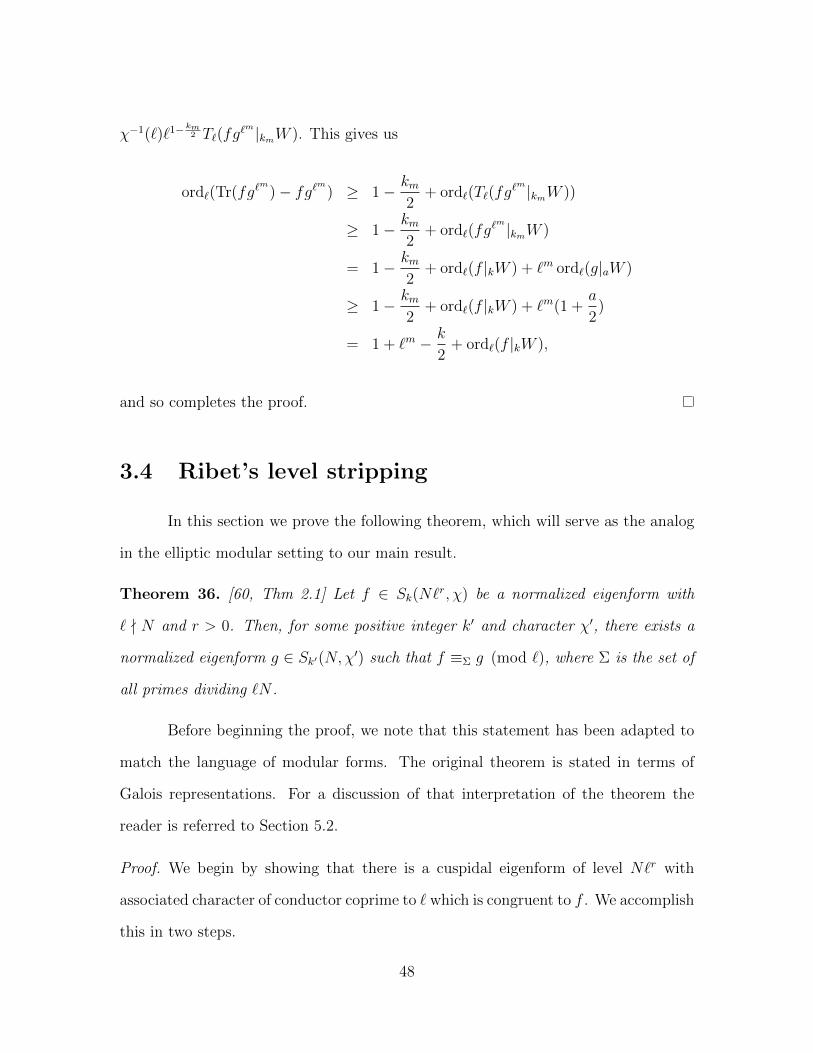
χ−1(`)`1− km2 T`(fg

`m |kmW ). This gives us

ord`(Tr(fg`m

)− fg`m) ≥ 1− km2

+ ord`(T`(fg`m|kmW ))

≥ 1− km2

+ ord`(fg`m|kmW )

= 1− km2

+ ord`(f |kW ) + `m ord`(g|aW )

≥ 1− km2

+ ord`(f |kW ) + `m(1 +a

2)

= 1 + `m − k

2+ ord`(f |kW ),

and so completes the proof.

3.4 Ribet’s level stripping

In this section we prove the following theorem, which will serve as the analog

in the elliptic modular setting to our main result.

Theorem 36. [60, Thm 2.1] Let f ∈ Sk(N`r, χ) be a normalized eigenform with

` - N and r > 0. Then, for some positive integer k′ and character χ′, there exists a

normalized eigenform g ∈ Sk′(N,χ′) such that f ≡Σ g (mod `), where Σ is the set of

all primes dividing `N .

Before beginning the proof, we note that this statement has been adapted to

match the language of modular forms. The original theorem is stated in terms of

Galois representations. For a discussion of that interpretation of the theorem the

reader is referred to Section 5.2.

Proof. We begin by showing that there is a cuspidal eigenform of level N`r with

associated character of conductor coprime to ` which is congruent to f . We accomplish

this in two steps.

48

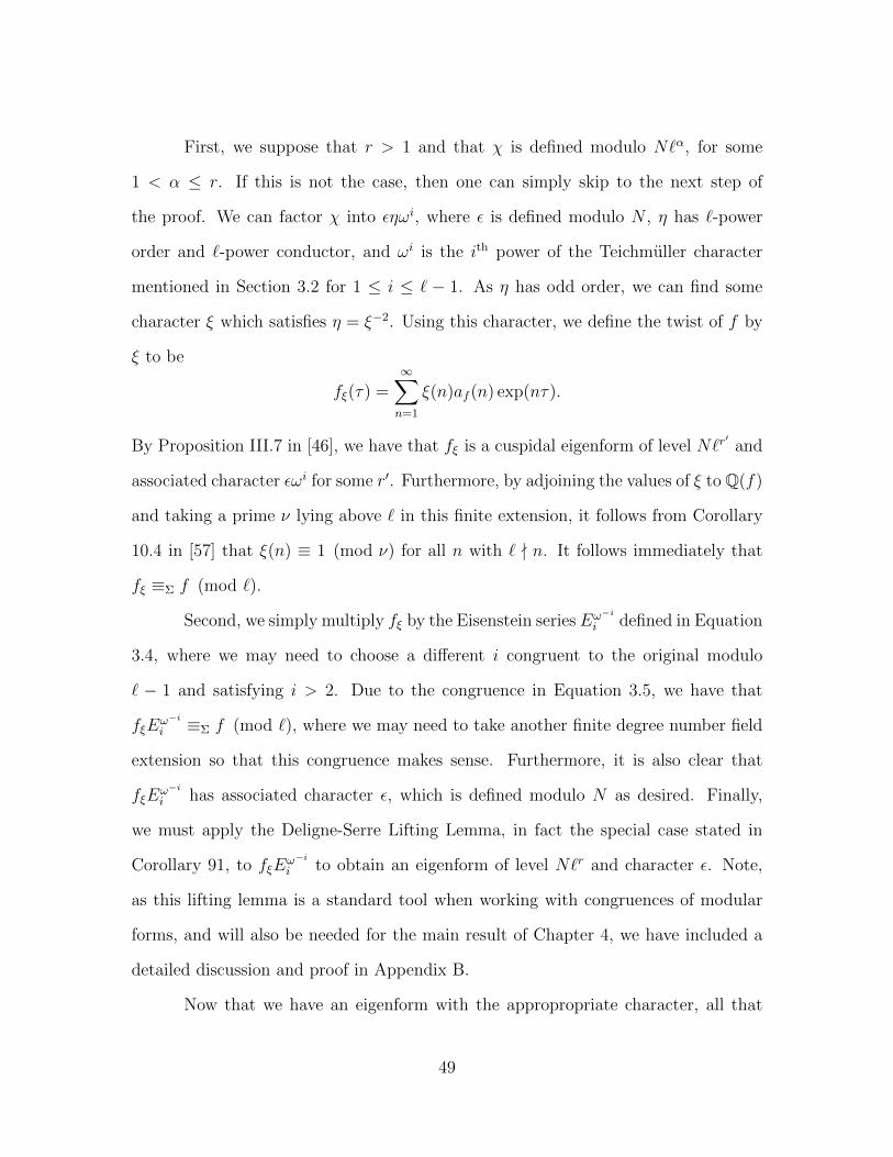
First, we suppose that r > 1 and that χ is defined modulo N`α, for some

1 < α ≤ r. If this is not the case, then one can simply skip to the next step of

the proof. We can factor χ into εηωi, where ε is defined modulo N , η has `-power

order and `-power conductor, and ωi is the ith power of the Teichmuller character

mentioned in Section 3.2 for 1 ≤ i ≤ ` − 1. As η has odd order, we can find some

character ξ which satisfies η = ξ−2. Using this character, we define the twist of f by

ξ to be

fξ(τ) =∞∑n=1

ξ(n)af (n) exp(nτ).

By Proposition III.7 in [46], we have that fξ is a cuspidal eigenform of level N`r′

and

associated character εωi for some r′. Furthermore, by adjoining the values of ξ to Q(f)

and taking a prime ν lying above ` in this finite extension, it follows from Corollary

10.4 in [57] that ξ(n) ≡ 1 (mod ν) for all n with ` - n. It follows immediately that

fξ ≡Σ f (mod `).

Second, we simply multiply fξ by the Eisenstein series Eω−ii defined in Equation

3.4, where we may need to choose a different i congruent to the original modulo

` − 1 and satisfying i > 2. Due to the congruence in Equation 3.5, we have that

fξEω−ii ≡Σ f (mod `), where we may need to take another finite degree number field

extension so that this congruence makes sense. Furthermore, it is also clear that

fξEω−ii has associated character ε, which is defined modulo N as desired. Finally,

we must apply the Deligne-Serre Lifting Lemma, in fact the special case stated in

Corollary 91, to fξEω−ii to obtain an eigenform of level N`r and character ε. Note,

as this lifting lemma is a standard tool when working with congruences of modular

forms, and will also be needed for the main result of Chapter 4, we have included a

detailed discussion and proof in Appendix B.

Now that we have an eigenform with the appropropriate character, all that

49

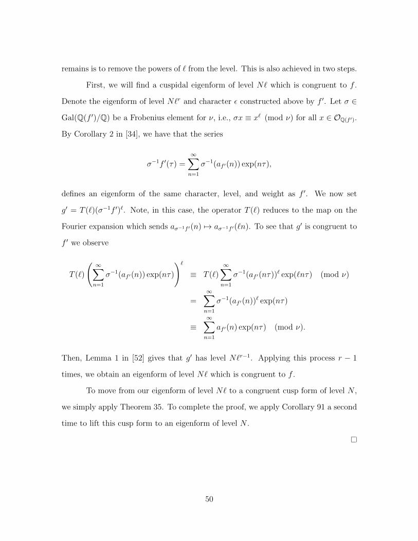
remains is to remove the powers of ` from the level. This is also achieved in two steps.

First, we will find a cuspidal eigenform of level N` which is congruent to f .

Denote the eigenform of level N`r and character ε constructed above by f ′. Let σ ∈

Gal(Q(f ′)/Q) be a Frobenius element for ν, i.e., σx ≡ x` (mod ν) for all x ∈ OQ(f ′).

By Corollary 2 in [34], we have that the series

σ−1f ′(τ) =∞∑n=1

σ−1(af ′(n)) exp(nτ),

defines an eigenform of the same character, level, and weight as f ′. We now set

g′ = T (`)(σ−1f ′)`. Note, in this case, the operator T (`) reduces to the map on the

Fourier expansion which sends aσ−1f ′(n) 7→ aσ−1f ′(`n). To see that g′ is congruent to

f ′ we observe

T (`)

(∞∑n=1

σ−1(af ′(n)) exp(nτ)

)`

≡ T (`)∞∑n=1

σ−1(af ′(nτ))` exp(`nτ) (mod ν)

=∞∑n=1

σ−1(af ′(n))` exp(nτ)

≡∞∑n=1

af ′(n) exp(nτ) (mod ν).

Then, Lemma 1 in [52] gives that g′ has level N`r−1. Applying this process r − 1

times, we obtain an eigenform of level N` which is congruent to f .

To move from our eigenform of level N` to a congruent cusp form of level N ,

we simply apply Theorem 35. To complete the proof, we apply Corollary 91 a second

time to lift this cusp form to an eigenform of level N .

50

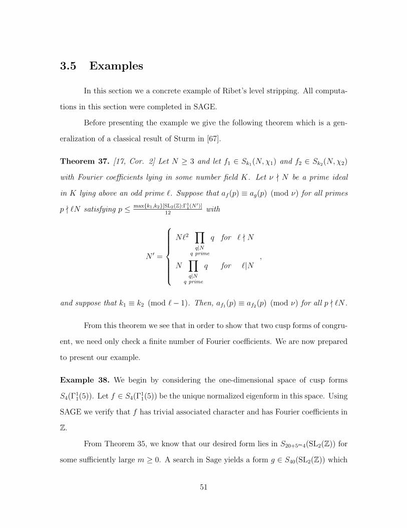
3.5 Examples

In this section we a concrete example of Ribet’s level stripping. All computa-

tions in this section were completed in SAGE.

Before presenting the example we give the following theorem which is a gen-

eralization of a classical result of Sturm in [67].

Theorem 37. [17, Cor. 2] Let N ≥ 3 and let f1 ∈ Sk1(N,χ1) and f2 ∈ Sk2(N,χ2)

with Fourier coefficients lying in some number field K. Let ν - N be a prime ideal

in K lying above an odd prime `. Suppose that af (p) ≡ ag(p) (mod ν) for all primes

p - `N satisfying p ≤ max{k1,k2}[SL2(Z):Γ11(N ′)]

12with

N ′ =

N`2∏q|N

q prime

q for ` - N

N∏q|N

q prime

q for `|N,

and suppose that k1 ≡ k2 (mod `− 1). Then, af1(p) ≡ af2(p) (mod ν) for all p - `N .

From this theorem we see that in order to show that two cusp forms of congru-

ent, we need only check a finite number of Fourier coefficients. We are now prepared

to present our example.

Example 38. We begin by considering the one-dimensional space of cusp forms

S4(Γ11(5)). Let f ∈ S4(Γ1

1(5)) be the unique normalized eigenform in this space. Using

SAGE we verify that f has trivial associated character and has Fourier coefficients in

Z.

From Theorem 35, we know that our desired form lies in S20+5m4(SL2(Z)) for

some sufficiently large m ≥ 0. A search in Sage yields a form g ∈ S40(SL2(Z)) which

51

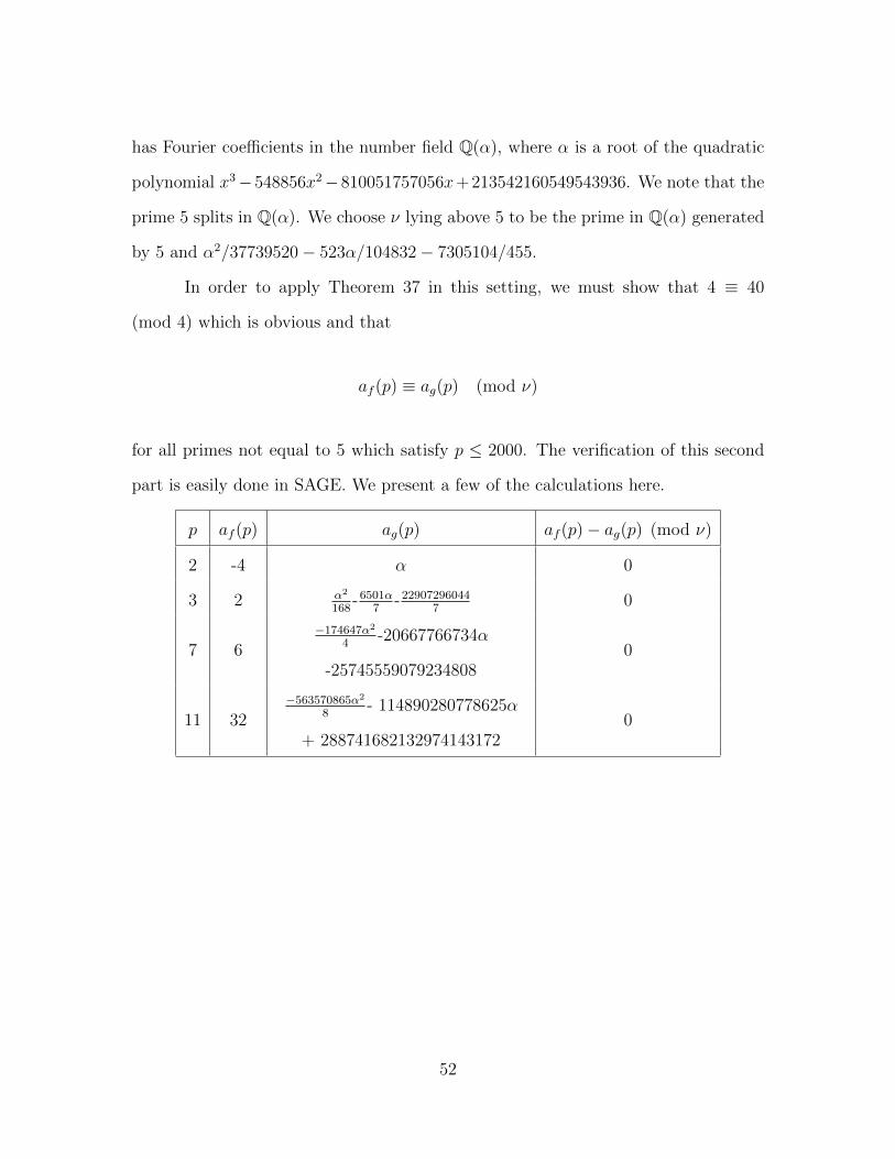
has Fourier coefficients in the number field Q(α), where α is a root of the quadratic

polynomial x3−548856x2−810051757056x+213542160549543936. We note that the

prime 5 splits in Q(α). We choose ν lying above 5 to be the prime in Q(α) generated

by 5 and α2/37739520− 523α/104832− 7305104/455.

In order to apply Theorem 37 in this setting, we must show that 4 ≡ 40

(mod 4) which is obvious and that

af (p) ≡ ag(p) (mod ν)

for all primes not equal to 5 which satisfy p ≤ 2000. The verification of this second

part is easily done in SAGE. We present a few of the calculations here.

p af (p) ag(p) af (p)− ag(p) (mod ν)

2 -4 α 0

3 2 α2

168-6501α

7-22907296044

70

7 6−174647α2

4-20667766734α

-257455590792348080

11 32−563570865α2

8- 114890280778625α

+ 2887416821329741431720

52

Chapter 4

Level stripping for genus 2 Siegel

modular forms

In this chapter, we present our main result. Throughout, we let ` > 3 denote

an odd rational prime.

4.1 Congruences of genus 2 Siegel modular forms

In this section we define two distinct notions of congruences between genus 2

Siegel modular forms. We then show a relationship between these two notions.

Let F and G be genus 2 eigenforms of level N and M respectively. For any

prime p - MN , we let λF (p), λF (p2; i), λG(p), λG(p2; i) denote the eigenvalues of F

and G with respect to T (p) and Ti(p2) for i = 1, 2, i.e.,

T (p)F = λF (p)F , Ti(p2)F = λF (p2; i)F,

T (p)G = λG(p)G, Ti(p2)G = λG(p2; i)G.

53

We let Q(λF , λG) denote the compositum of Q(λF ) and Q(λG), where Q(λF ) and

Q(λG) were defined in Lemma 27. By Lemma 27, Q(λF , λG) is a totally real number

field. Let Σ denote a finite set of primes. Then, we write F ≡Σ G (mod `) if for all

primes p /∈ Σ we have

λF (p) ≡ λG(p) (mod ν), λF (p2; i) ≡ λG(p2; i) (mod ν) for i = 1, 2,

where ν is a prime lying above ` in Q(λF , λG). This is referred to as a congruence of

eigenvalues.

Our second notion will be the congruence of Fourier coefficients, which we

define as in [9]. Before we can make sense of this notion, we will need the following

lemma.

Lemma 39. Let F ∈ S2ρ(N,χ) be an eigenform and let K denote Q(λF , χ), i.e., the

field obtained by adjoining all of the values of χ to Q(λF ). Set

S2ρ(N,χ;F ) =

{G ∈ S2

ρ(N,χ) : λG(t) = λF (t) for all t ∈ HZN(Γ2

0(N))}.

Then,

S2ρ(N,χ;F ) = S2

ρ(N,χ;F )OKL ⊗OKL C,

where OKL is the ring of integers of the compositum of K and L where L/Q is some

finite extension.

Proof. Recall, by Lemma 2.1 in [71] we have

S2ρ(N,χ) = S2

ρ(N,χ)OL ⊗OL C,

where we are using the same notation which was defined before Corollary 26 and

54

L/Q is a finite abelian extension. We assume that L contains the values of χ. Let

{F1, . . . , Fr} be a OL-basis for S2ρ(N,χ)OL . By Theorem 26, we have that

tFi =r∑j=1

cij(t)Fj for all t ∈ HZN(Γ2

0(N)),

where cij(t) ∈ OL.

For each z = (z1, . . . , zr) ∈ Cr we put

f(z) =r∑i=1

ziFi.

We set V (F ) = {z ∈ Cr : f(z) ∈ S2ρ(N,χ;F )}. Note, V (F ) is a finite dimensional

C-vector space and we denote the dimension by d. It is clear that f defines a C-linear

isomorphism

f : V (F )→ S2ρ(N,χ;F ).

Take S to be a generating set for HZN as a Z-algebra , which we know is finite because

HZN ↪→ EndC(S2

ρ(N,χ)). For z ∈ V (F ) it is clear that tf(z) = λF (t)f(z) for all t ∈ S,

i.e.,r∑i=1

cij(t)zi = λF (t)zi.

Since the coefficients λF (t), cij(t) are in KL, there exists a basis {v1, . . . , vd} of V (F )

such that vj ∈ (KL)r. Take a non-zero γj ∈ OKL such that v′j = γjvj ∈ OrKL. Then,

f(v′j) ∈ Snk (N,χ;F )OKL and V (F ) =⊕d

i=1 Cv′i.

Define the following field,

Q(F ) =∏T∈Λ2

Q(aF (T )),

55

where

Q(aF (T )) := Q

({aij : aF (T ) =

∑i,j

aijxi1x

j2

}).

As in Section 2.3, we have identified V with the homogeneous polynomials of degree

k2 − k1 in C[x1, x2], where (k1, k2) is the highest weight vector of ρ. Then, the

previous lemma gives that after some normalization, we may assume that Q(F ) is a

finite extension. We make the same assumption for the field Q(G).

We are now prepared to define the congruence of Fourier coefficients. Define

the `-adic valuation of F as

ord`(F ) = infT∈Λ2

{ordν(aF (T ))} ,

where

ordν(aF (T )) = mini,j

{ordν(aij) : aF (T ) =

∑i,j

aijxi1x

j2

},

and ν is prime lying above ` in Q(F ). Using this, we say that F and G have congruent

Fourier coefficients, denoted F ≡fc G (mod `r), if ord`(F −G) ≥ r.

For the genus 1 case, it is clear that these two notions of congruence are equiv-

alent, as the Fourier coefficients of a normalized elliptic eigenform are precisely the

eigenvalues. This equivalence is not necessarily true for any higher genus. However,

we do have the following lemma, which gives that a congruence of Fourier coefficients

implies a congruence of eigenvalues.

Lemma 40. Let F,G,Σ be as defined above. If F ≡fc G (mod `) then F ≡Σ G

(mod `).

Proof. This proof follows the same argument as in Theorem A.1 in [56], however we

include it here to emphasize that this result works for vector-valued forms of arbitrary

level, not just the classical forms of level one case as was proven in [56].

56

Define K to be the compositum of Q(F ) and Q(G). Also, we adjoin the values

of the characters of F and G if necessary and continue to denote this field by K. Let

c ∈ K so that at least one component of one Fourier coefficient of cF is an `-unit, i.e.,

for some T ∈ Λ2 and i, j ∈ N we have that ordν(aij) = 0, where aF (T ) =∑

i,j aijxi1x

j2

and ν is a prime lying above ` in K. Without loss of generality, we replace F and G

by cF and cG, respectively. Denote this component by aF (T )ij. Let t ∈ HZN(Γ2

0(N))

with tF = λF (t)F and tG = λG(t)G. Define the form H = F −G. Then,

λF (t)F − λG(t)G = t(F −G) = tH.

By Theorem 26, we have that Q(tH) ⊆ K. Hence,

λF (t)aF (T )ij ≡ λG(t)aG(T )ij (mod ν),

where ν is a prime lying above ` inK. Since aF (T )ij is an `-unit and aF (T )ij ≡ aG(T )ij

(mod ν), we have that λF (t) ≡ λG(t) (mod ν), which completes the proof.

4.2 A certain Eisenstein series

In this section, we give the construction of a degree 2 Eisenstein series which is

congruent to 1 (mod `). Note, this construction is due to Kikuta, see [45]. We include

the details of this construction not only because the techniques used are interesting

in their own right, but also because the proof of this theorem may provide a method

for generalizing our main result, which we will mention in later sections.

In fact, our main goal of this section is to provide a proof of the following

theorem.

57

Theorem 41. [45, Thm. 1.2] Let 1 ≤ i ≤ `. There exists a sequence {Gkm ∈

M2km

(`, ωi)} such that

limm→∞

Gkm = 1,

where the limit is taken `-adically with respect to the Fourier coefficients, ω is Te-

ichmuller character, and the sequence {km} will be defined later in this section.

We also give the following corollary which is what we will need for our main

result.

Corollary 42. For an integer k from the sequence {km}, there exists a G ∈M2k (`, ωi)

such that G ≡ 1 (mod `), where ω is the Teichmuller character and i is an integer

modulo `− 1.

Proof. Note, as the sequence {Gkm} converges `-adically to 1 as m → ∞, we have

that for every ε > 0, there is some M such that |Gkm − 1|` < ε for every m > M . By

definition of the `-adic absolute value this means that `− ord`(Gkm−1) < ε for every m >

M . As the choice of ε is arbitrary, we can find some Gkm such that ord`(Gkm−1) > 1,

i.e., Gkm ≡ 1 (mod `).

Before beginning the proof we fix an embedding

Q(µ`−1) ↪→ Q`,

where µ`−1 is the group of `− 1 roots of unity. To accomplish this we fix a primitive

element of µ`−1 which we will denote by ζ`−1. We want to consider the factorization

of ` in Z[ζ`−1]. Let Φ(x) denote the cyclotomic polynomial which has ζ`−1 as a root.

Then

Φ(x) ≡ p1(x) . . . pr(x) (mod `),

58

where r = φ(` − 1) and the pi(x) are all distinct degree 1 polynomials. Then, `

decomposes as a product of r prime ideals λi = (pi(ζ`−1), `). If we write pi(x) =

x − di, then we obtain an embedding σi : Q(ζ`−1) ↪→ Q` associated to λi by setting

ζσi`−1 = ω(di). In the following proof we fix one such embedding and denote it by σ.

We also set X = Z` × Z/(` − 1)Z, which we refer to as the group of weights,

as defined in [63]. Roughly speaking, if we have a sequence of elliptic modular forms

which converge `-adically, then the corresponding weights converge to an element of

X. For a more precise statement of this result, the reader is referred to Theoreme

1.4.2 in [63].

Proof of Theorem 41. Let EJk,1 denote the normalized Jacobi Eisenstein series of weight

k and index 1, which was introduced in Example 14. This EJk,1 has Fourier coefficients

in Q. Furthermore, we let Ek and Ek,ωi be defined as in Example 4 and Equation

3.4, respectively. From Chapter 2, we know that Ek has Fourier coefficients in Q and

Ek,ωi has Fourier coefficients in Q(µ`−1).

Define the sequence {km = a`m+1} for 0 < a ∈ Z, which satisfy a ≡ −i

(mod `− 1).

If we set

φkm(τ, z) = E1a(`−2),ωi(τ)E1

a`(`m−1)(τ)EJ2a,1(τ, z),

then φkm is Jacobi form of index 1, level ` and weight km. It is clear that in the

Fourier expansion

φkm(τ, z) =∑n,r

c(n, r) exp(nτ + rz),

we have c(n, r) ∈ Q(µ`−1) and c(0, 0) = 1.

We now need the following lemma.

59

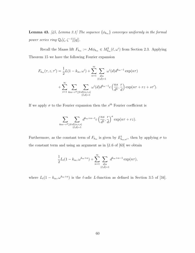
Lemma 43. [45, Lemma 3.1] The sequence {φkm} converges uniformly in the formal

power series ring Q`[ζ, ζ−1][[q]].

Recall the Maass lift Fkm :=Mφkm ∈ M2km

(`, ωi) from Section 2.3. Applying

Theorem 15 we have the following Fourier expansion

Fkm(τ, z, τ ′) =1

2L(1− km, ωi) +

∞∑n=1

∑d|n

(`,d)=1

ωi(d)dkm−1 exp(nτ)

+∞∑s=1

∑4ns−r2≥0

∑d|(n,r,s)(`,d)=1

ωi(d)dkm−1c(nsd2,r

d

)exp(nτ + rz + sτ ′).

If we apply σ to the Fourier expansion then the sth Fourier coefficient is

∑4ns−r2≥0

∑d|(n,r,s)(`,d)=1

dkm+α−1c(nsd2,r

d

)σexp(nτ + rz).

Furthermore, as the constant term of Fkm is given by E1km,ωi

, then by applying σ to

the constant term and using an argument as in §1.6 of [63] we obtain

1

2L`(1− km, ωkm+α) +

∞∑n=1

∑d|n

(`,d)=1

dkm+α−1 exp(nτ),

where L`(1 − km, ωkm+α) is the `-adic L-function as defined in Section 3.5 of [34].

60

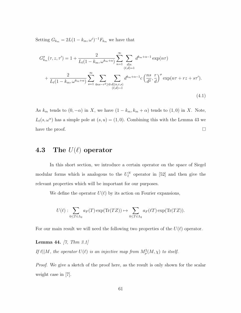
Setting Gkm = 2L(1− km, ωi)−1Fkm we have that

Gσkm(τ, z, τ ′) = 1 +

2

L`(1− km, ωkm+α)

∞∑n=1

∑d|n

(`,d)=1

dkm+α−1 exp(nτ)

+2

L`(1− km, ωkm+α)

∞∑s=1

∑4ns−r2≥0

∑d|(n,r,s)(`,d)=1

dkm+α−1c(nsd2,r

d

)σexp(nτ + rz + sτ ′).

(4.1)

As km tends to (0,−α) in X, we have (1 − km, km + α) tends to (1, 0) in X. Note,

L`(s, ωu) has a simple pole at (s, u) = (1, 0). Combining this with the Lemma 43 we

have the proof.

4.3 The U(`) operator

In this short section, we introduce a certain operator on the space of Siegel

modular forms which is analogous to the UN` operator in [52] and then give the

relevant properties which will be important for our purposes.

We define the operator U(`) by its action on Fourier expansions,

U(`) :∑

0≤T∈Λ2

aF (T ) exp(Tr(TZ)) 7→∑

0≤T∈Λ2

aF (`T ) exp(Tr(TZ)).

For our main result we will need the following two properties of the U(`) operator.

Lemma 44. [7, Thm 3.1]

If `||M , the operator U(`) is an injective map from M2ρ (M,χ) to itself.

Proof. We give a sketch of the proof here, as the result is only shown for the scalar

weight case in [7].

61

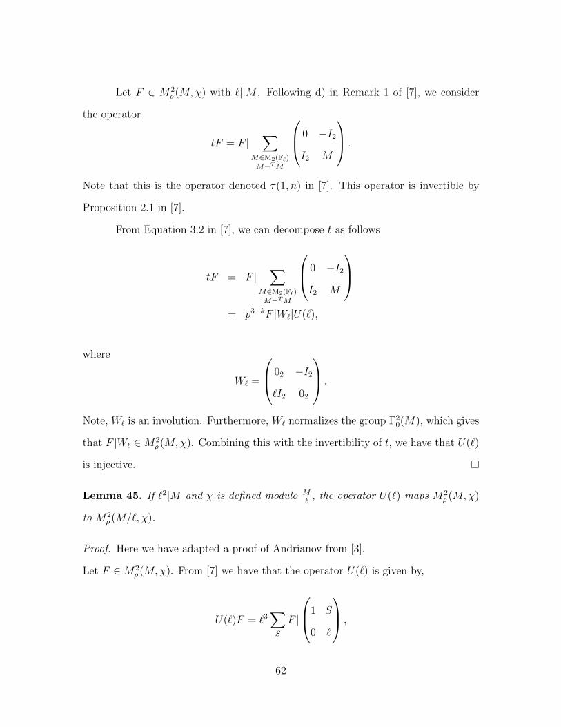
Let F ∈ M2ρ (M,χ) with `||M . Following d) in Remark 1 of [7], we consider

the operator

tF = F |∑

M∈M2(F`)M=TM

0 −I2

I2 M

.

Note that this is the operator denoted τ(1, n) in [7]. This operator is invertible by

Proposition 2.1 in [7].

From Equation 3.2 in [7], we can decompose t as follows

tF = F |∑

M∈M2(F`)M=TM

0 −I2

I2 M

= p3−kF |W`|U(`),

where

W` =

02 −I2

`I2 02

.

Note, W` is an involution. Furthermore, W` normalizes the group Γ20(M), which gives

that F |W` ∈M2ρ (M,χ). Combining this with the invertibility of t, we have that U(`)

is injective.

Lemma 45. If `2|M and χ is defined modulo M`

, the operator U(`) maps M2ρ (M,χ)

to M2ρ (M/`, χ).

Proof. Here we have adapted a proof of Andrianov from [3].

Let F ∈M2ρ (M,χ). From [7] we have that the operator U(`) is given by,

U(`)F = `3∑S

F |

1 S

0 `

,

62

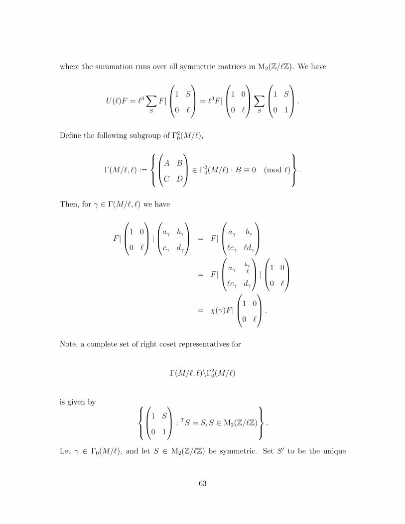
where the summation runs over all symmetric matrices in M2(Z/`Z). We have

U(`)F = `3∑S

F |

1 S

0 `

= `3F |

1 0

0 `

∑S

1 S

0 1

.

Define the following subgroup of Γ20(M/`),

Γ(M/`, `) :=

A B

C D

∈ Γ20(M/`) : B ≡ 0 (mod `)

.

Then, for γ ∈ Γ(M/`, `) we have

F |

1 0

0 `

|aγ bγ

cγ dγ

= F |

aγ bγ

`cγ `dγ

= F |

aγbγ`

`cγ dγ

|1 0

0 `

= χ(γ)F |

1 0

0 `

.

Note, a complete set of right coset representatives for

Γ(M/`, `)\Γ20(M/`)

is given by 1 S

0 1

: TS = S, S ∈ M2(Z/`Z)

.

Let γ ∈ Γ0(M/`), and let S ∈ M2(Z/`Z) be symmetric. Set S ′ to be the unique

63

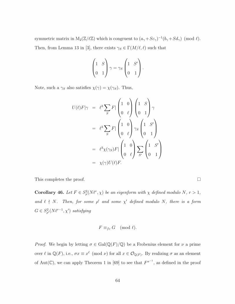
symmetric matrix in M2(Z/`Z) which is congruent to (aγ+Scγ)−1(bγ+Sdγ) (mod `).

Then, from Lemma 13 in [3], there exists γS ∈ Γ(M/`, `) such that

1 S

0 1

γ = γS

1 S ′

0 1

.

Note, such a γS also satisfies χ(γ) = χ(γS). Thus,

U(`)F |γ = `3∑S

F |

1 0

0 `

1 S

0 1

γ

= `3∑S

F |

1 0

0 `

γS

1 S ′

0 1

= `3χ(γS)F |

1 0

0 `

∑S′

1 S ′

0 1

= χ(γ)U(`)F.

This completes the proof.

Corollary 46. Let F ∈ S2ρ(N`

r, χ) be an eigenform with χ defined modulo N , r > 1,

and ` - N . Then, for some ρ′ and some χ′ defined modulo N , there is a form

G ∈ S2ρ′(N`

r−1, χ′) satisfying

F ≡fc G (mod `).

Proof. We begin by letting σ ∈ Gal(Q(F )/Q) be a Frobenius element for ν a prime

over ` in Q(F ), i.e., σx ≡ x` (mod ν) for all x ∈ OQ(F ). By realizing σ as an element

of Aut(C), we can apply Theorem 1 in [69] to see that F σ−1, as defined in the proof

64

of Lemma 27, is an eigenform in S2ρ(N`

r, σ−1 ◦ χ). Define a form G = U(`)(F σ−1)`.

Then, just as in the proof of Theorem 36, we have

U(`)

∑T>0T∈Λ2

σ−1(aF (T )) exp(Tr(TZ))

`

≡ U(`)∑T>0T∈Λ2

σ−1(aF (T ))` exp(`Tr(TZ)) (mod ν)

=∑T>0T∈Λ2

σ−1(aF (T ))` exp(Tr(TZ))

≡∑T>0T∈Λ2

aF (T ) exp(Tr(TZ)) (mod ν).

Thus, G is congruent in Fourier coefficients to F . Moreover, by Lemma 45, G ∈

S2ρ′(N`

r−1, χ′) for some ρ′ and χ′.

4.4 Theta series

In this section, we introduce a certain family of theta series which satisfy a

certain congruence. We follow [10], [11] throughout this section.

We begin with some preliminary definitions.

Definition 47. Let V be a vector space and let Q be a quadratic form defined on V .

Then, we call (V,Q) a quadratic space. Furthermore, we say that (V,Q) is positive

definite if Q(v) > 0 for all v ∈ V .

We assume throughout that our quadratic spaces are defined over Q of dimen-

sion d, i.e., V is a vector space over Q of dimension d.

Associated to any quadratic form we have a natural bilinear form given by

(v1, v2) = Q(v1 + v2)−Q(v1)−Q(v2).

65

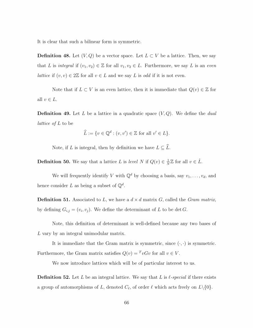
It is clear that such a bilinear form is symmetric.

Definition 48. Let (V,Q) be a vector space. Let L ⊂ V be a lattice. Then, we say

that L is integral if (v1, v2) ∈ Z for all v1, v2 ∈ L. Furthermore, we say L is an even

lattice if (v, v) ∈ 2Z for all v ∈ L and we say L is odd if it is not even.

Note that if L ⊂ V is an even lattice, then it is immediate that Q(v) ∈ Z for

all v ∈ L.

Definition 49. Let L be a lattice in a quadratic space (V,Q). We define the dual

lattice of L to be

L := {v ∈ Qd : (v, v′) ∈ Z for all v′ ∈ L}.

Note, if L is integral, then by definition we have L ⊆ L.

Definition 50. We say that a lattice L is level N if Q(v) ∈ 1NZ for all v ∈ L.

We will frequently identify V with Qd by choosing a basis, say v1, . . . , vd, and

hence consider L as being a subset of Qd.

Definition 51. Associated to L, we have a d× d matrix G, called the Gram matrix,

by defining Gi,j = (vi, vj). We define the determinant of L to be detG.

Note, this definition of determinant is well-defined because any two bases of

L vary by an integral unimodular matrix.

It is immediate that the Gram matrix is symmetric, since (·, ·) is symmetric.

Furthermore, the Gram matrix satisfies Q(v) = TvGv for all v ∈ V .

We now introduce lattices which will be of particular interest to us.

Definition 52. Let L be an integral lattice. We say that L is `-special if there exists

a group of automorphisms of L, denoted C`, of order ` which acts freely on L\{0}.

66

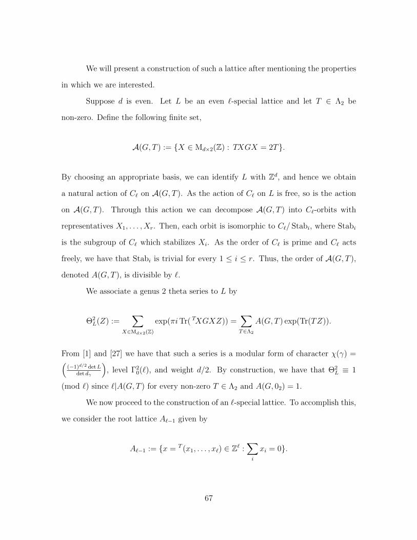
We will present a construction of such a lattice after mentioning the properties

in which we are interested.

Suppose d is even. Let L be an even `-special lattice and let T ∈ Λ2 be

non-zero. Define the following finite set,

A(G, T ) := {X ∈ Md×2(Z) : TXGX = 2T}.

By choosing an appropriate basis, we can identify L with Zd, and hence we obtain

a natural action of C` on A(G, T ). As the action of C` on L is free, so is the action

on A(G, T ). Through this action we can decompose A(G, T ) into C`-orbits with

representatives X1, . . . , Xr. Then, each orbit is isomorphic to C`/ Stabi, where Stabi

is the subgroup of C` which stabilizes Xi. As the order of C` is prime and C` acts

freely, we have that Stabi is trivial for every 1 ≤ i ≤ r. Thus, the order of A(G, T ),

denoted A(G, T ), is divisible by `.

We associate a genus 2 theta series to L by

Θ2L(Z) :=

∑X∈Md×2(Z)

exp(πiTr( TXGXZ)) =∑T∈Λ2

A(G, T ) exp(Tr(TZ)).

From [1] and [27] we have that such a series is a modular form of character χ(γ) =((−1)d/2 detL

det dγ

), level Γ2

0(`), and weight d/2. By construction, we have that Θ2L ≡ 1

(mod `) since `|A(G, T ) for every non-zero T ∈ Λ2 and A(G, 02) = 1.

We now proceed to the construction of an `-special lattice. To accomplish this,

we consider the root lattice A`−1 given by

A`−1 := {x = T (x1, . . . , x`) ∈ Z` :∑i

xi = 0}.

67

From §6 in [19], we have that this is an even lattice of rank ` − 1, level `, and

determinant `. The symmetric group, S`, acts on A`−1 by permuting the coordinates.

Suppose that σ ∈ S` has a nontrivial fixed point x ∈ A`−1. Divide the indices

of x into two sets by defining M+ := {i : xi ≥ 0} and M− := {i : xi < 0}. Then,

M+ and M− are stable under the action of σ, i.e., we can view σ as an element of

Sr×S`−r, where the order of M+ is r. In particular, σ cannot be an element of order

`. Thus, we have that any `-Sylow subgroup of S` acts freely on R`−1\{0}. Therefore,

A`−1 is an `-special lattice.

For our purposes, we will need the lattice L = A`−1

⊕A`−1, which is `-special

when equipped with the diagonal action of a `-Sylow subgroup of S`. Note, L has

rank 2`− 2, level `, and determinant `2. Thus, we have construced a form

Θ2L ∈M2

`−1(`, 1`), with Θ2L ≡ 1 (mod `), (4.2)

where we use 1` to denote the trivial character.

4.5 The trace operator

In this section, we introduce the trace operator from [8] in the genus 2 setting.

Let F ∈ S2ρ(N,χ) be a Siegel modular form of genus 2, and let Γ1 ⊂ Γ2 be

level N congruence subgroups of the type listed in Section 2.3. Then, we define the

trace of F to be

TrΓ2Γ1

(F ) :=1

[Γ2 : Γ1]

∑γ∈Γ1\Γ2

χ−1(γ)F |γ,

where the summation is taken over a complete set of coset representatives. Note,

when the levels are clear from context we will simply write Tr(F ). The following

proposition gives us an important result on the level of Tr(F ).

68

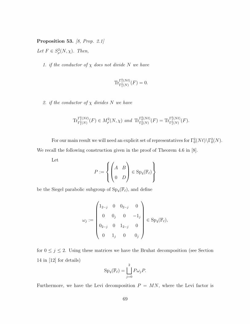
Proposition 53. [8, Prop. 2.1]

Let F ∈ S2ρ(N,χ). Then,

1. if the conductor of χ does not divide N we have

TrΓ21(N`)

Γ21(N)

(F ) = 0.

2. if the conductor of χ divides N we have

TrΓ21(N`)

Γ21(N)

(F ) ∈M2ρ (N,χ) and Tr

Γ20(N`)

Γ20(N)

(F ) = TrΓ21(N`)

Γ21(N)

(F ).

For our main result we will need an explicit set of representatives for Γ20(N`)\Γ2

0(N).

We recall the following construction given in the proof of Theorem 4.6 in [8].

Let

P :=

A B

0 D

∈ Sp4(F`)

be the Siegel parabolic subgroup of Sp4(F`), and define

ωj :=

12−j 0 02−j 0

0 0j 0 −1j

02−j 0 12−j 0

0 1j 0 0j

∈ Sp4(F`),

for 0 ≤ j ≤ 2. Using these matrices we have the Bruhat decomposition (see Section

14 in [12] for details)

Sp4(F`) =2⊔j=0

PωjP.

Furthermore, we have the Levi decomposition P = MN , where the Levi factor is

69

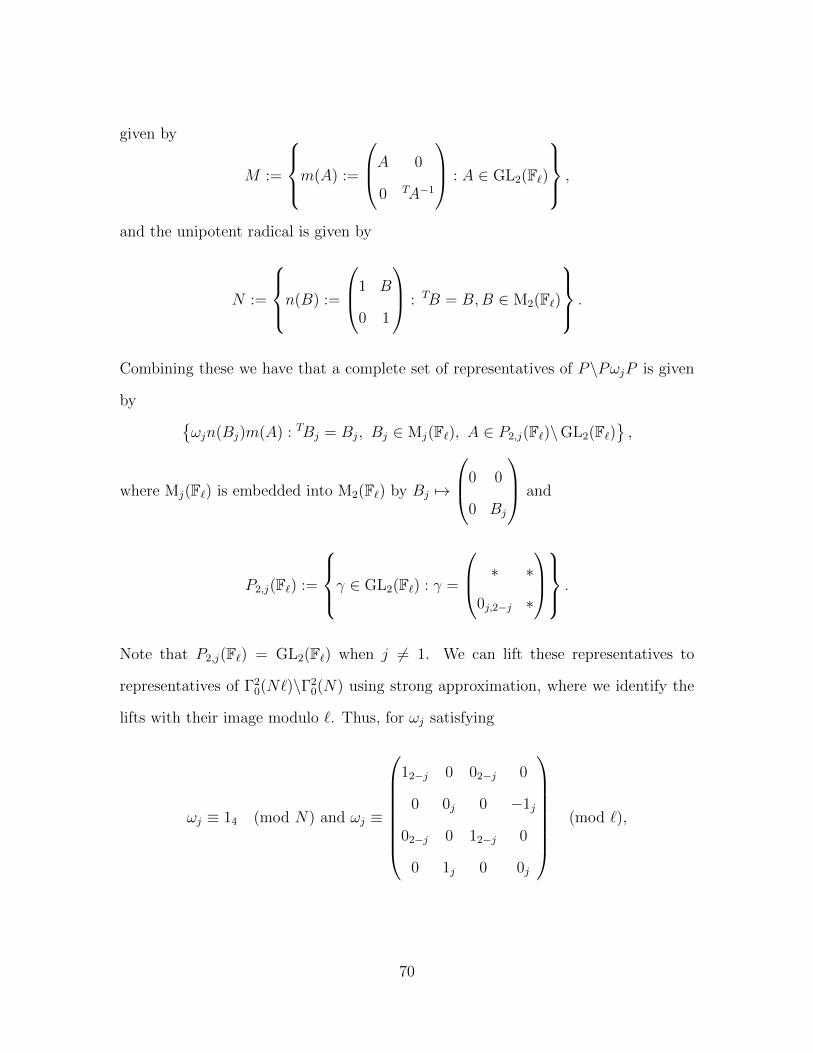
given by

M :=

m(A) :=

A 0

0 TA−1

: A ∈ GL2(F`)

,

and the unipotent radical is given by

N :=

n(B) :=

1 B

0 1

: TB = B,B ∈ M2(F`)

.

Combining these we have that a complete set of representatives of P\PωjP is given

by {ωjn(Bj)m(A) : TBj = Bj, Bj ∈ Mj(F`), A ∈ P2,j(F`)\GL2(F`)

},

where Mj(F`) is embedded into M2(F`) by Bj 7→

0 0

0 Bj

and

P2,j(F`) :=

γ ∈ GL2(F`) : γ =

∗ ∗

0j,2−j ∗

.

Note that P2,j(F`) = GL2(F`) when j 6= 1. We can lift these representatives to

representatives of Γ20(N`)\Γ2

0(N) using strong approximation, where we identify the

lifts with their image modulo `. Thus, for ωj satisfying

ωj ≡ 14 (mod N) and ωj ≡

12−j 0 02−j 0

0 0j 0 −1j

02−j 0 12−j 0

0 1j 0 0j

(mod `),

70

we have that

{ωjn(Bj)m(A) : 0 ≤ j ≤ 2}

is a complete set of representatives for Γ20(N`)\Γ2

0(N). Furthermore, we may assume

for our lifted m(A) that detA = 1. This gives us that χ−1 is trivial on our set of

representatives. Using these representatives we rewrite

Tr(F ) = F +`−1∑b=1

∑A

F |ω1n(b)m(A) +∑TB=B

B (mod `)

F |ω2n(B).

To complete this section, we give a more explicit expression for the last term

in the trace. Note that since F is a cusp form, we have that F |ω2 is also a cusp form.

In particular, we know that the Fourier expansion is of the following form,

(F |ω2)(Z) =∑T∈ 1

`Λ2

a(T ) exp(Tr(TZ)).

From [9] we have that

∑TB=B

B (mod `)

(F |ω2n(B))(Z) = `3∑T∈Λ2

a(T ) exp(Tr(TZ)).

Using this equality we obtain

∑TB=B

B (mod `)

F |ω2n(B) = `3F |ω2

`2 0

0 12

U(`).

We will need the following lemma, which is from [9], for the proof of our main result.

We prove it here for completeness.

71

Lemma 54. Let F ∈ S2ρ(N`, χ) be an eigenform with associated character χ defined

modulo N . Then, for some ρ′ there exists G ∈ S2ρ′(N,χ) such that F ≡fc G (mod `).

Proof. As we are only proving this for degree 2 Siegel modular forms, we will drop

the 2 from the superscript for the remainder of this proof.

By Lemma 44 we have that the Hecke operator U(`) is an injective map from

Sρ(N`, χ) into itself. As Sρ(N`, χ) is a finite dimensional vector space, this means that

U(`) is surjective as well. Thus, we can find a G′ ∈ Sρ(N`, χ) such that G′|U(`) = F .

Using this G′, define the following form

G = G′|

1`· 12 0

0 12

|ω−12 .

Let K`−1 := `2Θ2L, where Θ2

L is the theta series from Equation 4.2. Then, from [11],

we have that K`−1 satisfies

K`−1 ≡fc K`−1|ω1 ≡fc 0 (mod `),

K`−1|ω2 ≡fc 1 (mod `).

Furthermore, K`−1 has integral Fourier coefficients. Applying our formula for the

trace we may write

Tr(GK`m`−1) = GK`m`−1 +`−1∑b=1

∑A

(GK`m`−1)|ω1n(b)m(A)

+∑TB=B

B (mod `)

(GK`m`−1)|ω2n(B),

72

for an arbitrary constant m. Our goal is to show that

ord`(Tr(GK`m`−1))→∞ as m→∞.

To this end we will examine each piece of the sum separately and use the fact that

ord`(G|ωi) > −∞ for i = 0, 1, 2. This fact comes from Proposition 3.3 in [9].

First,

ord`(GK`m

`−1) = ord`(G) + `m ord`(K`−1),

which becomes arbitrarily large with m.

Second,

ord`

(`−1∑b=1

∑A

(GK`m`−1)|ω1n(b)m(A)

)≥ 1 + ord`(G|ω1) + `m ord`(K`−1|ω1),

which also becomes arbitrarily large with m.

Third, to examine the last term of the summation we rewriteK`m`−1 = 1+`m+1X,

where X is a Fourier series with integral Fourier coefficients. Then,

∑TB=B

B (mod `)

(GK`m`−1)|ω2n(B) = G|ω2|

` · 12 0

0 12

U(`)

+ `m+1(G|ω2 ·X)|

` · 12 0

0 12

U(`)

= F + `m+1(G|ω2 ·X)|

` · 12 0

0 12

U(`).

73

Note that ord`(X) ≥ 0. Combining we have,

ord`(F − Tr(GK`m`−1)) ≥ m+ 1 + ord`(G|ω2).

Which goes to infinity asm does. Thus, for large enoughm, we have that Tr(GK`m`−1) ≡fc

F (mod `).

4.6 Main result

In this section, we will prove the following theorem, which constitutes our

main result. Note, the corresponding result for scalar valued forms can be found in

[42].

Theorem 55. Let F ∈ S2ρ(`

rN,χ) be an eigenform with the highest weight vector

of ρ satisfying k2 ≥ 3 and χ defined modulo `N with ` - N . Let Σ be the set of

rational primes which divide `N . Then, for some χ′ and ρ′, there exists an eigenform

G ∈ S2ρ′(N,χ

′) such that F ≡Σ G (mod `).

Proof. Throughout we are working with degree 2 Siegel modular forms, so we will

drop the superscript. Furthermore, throughout the proof we will not be explicit about

the weights of the intermediate forms, but we will make a note about the final weight

ρ′ at the end. Finally, we will take finite extensions of Q as needed.

As χ is a character modulo `N we obtain a factorization χ = ωiκ, where ω is

the unique character of conductor ` and order ` − 1, i.e., the Teichmuller character,

and κ is a character modulo N .

Let E ∈ Mk(`, ω−i) be a form from the sequence in Theorem 41 such that

E ≡fc 1 (mod `). Consider the product of Siegel modular forms FE.

74

We first want to show that this product transforms correctly under the action

of Γ0(`r) ∩ Γ1(N). Let γ ∈ Γ0(`r) ∩ Γ1(N). Then,

(F (Z)E(Z))|γ = κωi(γ)ω−i(γ) det(cZ + d)−kρ(cZ + d)−1F (γZ)E(γZ)

= F (Z)E(Z).

Thus, the product is a form of the desired level and of character κ. We will denote

the weight of this form by ρ′. Furthermore, as E ≡fc 1 (mod `) we have that

FE ≡fc F (mod `).

Thus, FE is an eigenform when reduced modulo ν for a prime ν lying above ` in

Q(F ), and Lemma 40 gives us

FE ≡Σ F (mod `).

Let Oν be an extension of Z` which has ν as its maximal ideal. As Sρ′(N`r, κ) is

a finite, free Oν module, we can apply the Deligne-Serre lifting lemma as stated in

Corollary 91 to obtain an eigenform F1 ∈ Sρ′(N`r, κ) such that

F1 ≡Σ F (mod `).

We can now apply Corollary 46 (r − 1) times to F1 in order to obtain a form

F2 ∈ Sρ′(N`, χ′) for some ρ′ and χ′, which is congruent in Fourier coefficients modulo

` to F . By the same argument used above we can find an eigenform in Sρ′(N`, χ′)

satisfying this same congruence.

We now apply Lemma 54 to F2 to obtain a form F3 ∈ Sρ′(N,χ′) which is

75

congruent in Fourier coefficients to F modulo ν. Just as before, this yields the desired

eigenform G.

Finally, with regards to the weight ρ′ of G, if we let the highest weight vector

of ρ be (k1, k2), then the highest weight vector of ρ′ is

(`(k1 + i`m1 + `m2−1(`− 1)), `(k2 + i`m1 + `m2−1(`− 1)),

where m1 and m2 are both sufficiently large integers. In particular, we have that

(k′1, k′2) ≡ (k1 + i, k2 + i) (mod `− 1),

where (k′1, k′2) is the highest weight vector of ρ′.

4.7 Examples

We conclude this chapter by giving a computational example of the result in

Theorem 55.

In order to construct the example we will use the Saito-Kurokawa lift. We

suppress the details of this lift here but the reader is referred to [53], [54], and [58]

for classical and representation theoretic treatments of the Saito-Kurokawa lift.

Before giving our examples, we will present some necessary facts concerning

this lifting. Let f ∈ S12k−2(N,χ) be a normalized eigenform with χ = ψ2 for some

Dirichlet character ψ defined modulo N . Let Ff ∈ S2k(N,ψ) denote a Saito-Kurokawa

lift of f . Then, from Theorem 5.2 in [54] we have that the L-function associated to

76

Ff factors as

L(s, F ) =

∏p|N

(1− pk−1−s)(1− pk−2−s)

ζ(s− k + 1)ζ(s− k + 2)L(s, f).

From this factorization we can deduce the following relationship between the eigen-

values of Ff and f for p - N

λFf (p;S) = λf (p) + χ(p)pk−2(p+ 1),

λFf (p2;S) = χ(p)2p2k−6(p2 − 1) + χ(p)λf (p)p

k−3(p+ 1), (4.3)

where λFf (p;S) and λFf (p2;S) are eigenvalues with respect to certain Hecke opera-

tors TS(p) and TS(p2) which are defined in [4]. It should be noted that TS(p) and

TS(p2) also generate the local Hecke algebra Hp, so it is sufficient to work with these

operators.

Example 56. We construct our example by setting f ∈ S4(Γ11(5)) and g ∈ S40(SL2(Z))

be the forms given in Example 38.

From the above discussion, we have that the Saito-Kurokawa lift of f and

of g, which we denote by Ff and Fg, respectively, satisfy Ff ∈ S3(Γ21(5)) and Fg ∈

S21(Sp4(Z)). Furthermore, Ff and Fg are eigenforms with eigenvalues satisfying

Equation 4.3.

Due to the equations given in 4.3 and the fact that f and g are congruent

modulo 5, it is elementary to check that the eigenvalues of Ff and Fg are congruent

modulo 5.

77

Chapter 5

Applications to Galois

representations

In this chapter, we give a brief introduction to Galois representations and

provide some applications of the previous level stripping arguments to Galois repre-

sentations. Throughout, we will use GQ to denote Gal(Q/Q), and after fixing an odd

prime `, we fix embeddings Q ↪→ Q` and Q ↪→ C.

5.1 Galois representations

In this section, we introduce the basic objects of study and a few examples.

We begin by recalling the definition of a profinite group.

Definition 57. We say that a topological group G is a profinite group if it can be

expressed as the inverse limit of finite groups equipped with the discrete topology.

We refer to the topology of G as the profinite topology.

Note, if G = lim←i

Gi, where the Gi are finite groups equipped with the discrete

topology, then the topology of G is simply given as the subspace topology of the

78

product topology on∏

iGi. We consider two more explicit examples of this, both of

which will be used throughout the remainder of the chapter.

Example 58. 1. Consider the collection of finite groups {Z/`nZ : n ∈ Z+}, each

equipped with the discrete topology. We take the inverse limit of this collection

with respect to the reduction homomorphism Z/`nZ→ Z/`n−1Z to obtain the

`-adic integers

Z` = lim←n

Z/`nZ.

It is well known that Z` comes equipped with the absolute value

|a|` = `− ord`(a).

One can check that the topology induced by this absolute value agrees with the

profinite topology described above.

2. Consider the group GQ. We have that

GQ = lim←K

Gal(K/Q),

where each K/Q is a finite Galois extension and the inverse limit is taken

with respect to the restriction homomorphism Gal(K1/Q)→ Gal(K2/Q) when

K2 ⊆ K1. We have a topology on GQ given by the following basis of open sets,

{σGal(Q/K) : [K : Q] <∞, σ ∈ GQ

}.

This topology is referred to as the Krull topology, and once again, one can check

that this topology is equivalent to the profinite topology defined above.

We are now prepared to define the objects of primary interest.

79

Definition 59. Let d be a positive integer and ` an odd prime. Let K be either the

complex numbers or an extension of Q`. A d-dimensional Galois representation is a

continuous homomorphism

ρ : GQ → GL(V ),

where V is a d-dimensional K vector space and the topology on V is induced from

the topology on K. In the case that K = C, we call ρ an Artin representation, and

in the case that Q` ⊆ K, we call ρ an `-adic representation. Note, after choosing a

basis, we can assume that

ρ : GQ → GLd(K).

As GQ is equipped with the profinite topology and a finite dimensional C vector

space is equipped with the Euclidean topology, the continuity condition ensures that

the image of any Artin representation is finite. To see this, note that the identity

Id ∈ GLd(C) has an open neighborhood, denoted U , which contains no non-trivial

subgroup. By continuity, the pullback of U is an open neighborhood of the identity

in GQ, and since GQ is profinite the pullback contains a subgroup of finite index, say

UG. As ρ is a homomorphism, we have that ρ(UG) is a subgroup of GLd(C), and

hence UG ⊆ ker(ρ). Thus, ρ factors through a subgroup of finite index, so we must

have that the image of ρ is finite. We can think of this as implying that the topologies

of GQ and C are incompatible in some sense.

Due to this, we will be interested in `-adic Galois representations, and through-

out the remainder of the chapter, it should be assumed that all Galois representations

are `-adic. Note, in this case, GLd(K) comes equipped with the profinite topology as

well, and hence the continuity condition is not so restrictive in this setting as it is for

Artin representations.

We begin by giving some basic definitions and results concerning `-adic Galois

80

representations which will be useful to us.

Definition 60. If we let c ∈ GQ denote complex conjugation, then we say that ρ is

odd if

det ρ(c) = −1.

Definition 61. We say that ρ is irreducible if ρ has no nontrivial invariant subspaces.

Recall the following subgroups of GQ from algebraic number theory. Let p be

a prime in Z, the ring of integers of Q. Then, the decomposition group of p is

Dp = {σ ∈ GQ : σ(p) = p} ,

and the inertia group of p is given by

Ip ={σ ∈ Dp : σ(x) ≡ x (mod p) for all x ∈ Z

}.

Using the inertia group we are prepared to give the following definition.

Definition 62. Let p 6= ` be a rational prime. We say ρ is unramified at p if for any

maximal ideal p ⊂ Z lying over p, Ip is contained in the kernel of ρ.

Finally, we have the following standard definition from representation theory.

Definition 63. We say that ρ : GQ → GLd(K) is semi-simple if Kd can be written

as a direct sum of simple GQ-modules Ki, i.e., modules GQ-modules Ki such that Ki

has no proper submodule.

To expand on this last definition just a bit, we know that Kd has a composition

series of ρ-invariant subspaces, i.e.,

Kd = K0 ⊃ K1 ⊃ · · · ⊃ Kn = 0,

81

such that each Ki/Ki+1 is simple. Set

K ′ =n−1⊕i=0

Ki/Ki+1,

and use ρ to define a new representation

ρss : GQ →n−1⊕i=0

GL(Ki/Ki+1).

We call ρss the semi-simplification of ρ.

We also have the notion of isomorphic Galois representations. If ρ and ρ′ are

both d-dimensional Galois representations and there is some M ∈ GLd(K) which

satisfies

ρ′(σ) = M−1ρ(σ)M for all σ ∈ GQ,

then we say that ρ and ρ′ are isomorphic. We will need the following proposition,

as we will be interested in reducing the image of a Galois representation modulo a

prime.

Proposition 64. Let ρ : GQ → GLd(K) be an `-adic Galois representation. Then,

there exists a ρ′ : GQ → GLd(OK) such that ρ and ρ′ are isomorphic.

Proof. Let Λ = OdK . As Λ is a lattice of Kd, we have that Λ is compact in Kd. Since

ρ is continuous, we have that the map

Fρ : Kd ×GQ → Kd, given by (v, σ) 7→ ρ(σ) · v

is continuous. Hence, Λ′ := Fρ(Λ×GQ) is compact in Kd. Then, Λ′ lies in $−rΛ for

some r ∈ Z+, where $ is a uniformizer of OK . Since Λ′ contains Λ, the rank of Λ′ is

at least d. Furthermore, as OK is an integral domain, we have that Λ′ is free, and it

82

follows that the rank of Λ′ is d. Therefore, by choosing an OK basis of Λ′, we obtain

the desired representation

ρ′ : GQ → GLd(OK).

To conclude this section we will give a few well-known examples of Galois

representations.

Example 65. Consider the following sequence of maps

GQπ−→ Gal (Q(µ`)/Q)

∼−→ (Z/`Z)xω−→ Zx

`,

where µ` is a primitive `th root of unity, π is the projection to GQ/Gal(Q/Q(µ`)

) ∼=Gal (Q(µ`)/Q), and ω is the Teichmuller character. If we take the composition of

these maps, then we obtain the cyclotomic character at `, i.e.,

χ` : GQ → Zx`.

This is a continuous, one-dimensional, odd, `-adic Galois representation. Note, for

any rational prime p 6= `, we have that p is unramified in Q(µ`), i.e., for any ℘ lying

over p in Q(µ`) we have I℘ is trivial. Thus, I℘ ⊂ kerχ`, i.e., χ` is unramified at p. In

fact, for any maximal ideal p ⊂ Z lying over a rational prime p 6= `, we have

χ`(Frobp) = p,

where Frobp is the (arithmetic) Frobenius element at p in GQ. It is a consequence of

83

the continuity of χ` and the Chebotarov density theorem that the set

{Frobp ∈ GQ : p ∩ Z = p, p 6= `}

is dense in GQ, and hence χ` is completely determined by its image on this set.

Now, we will consider a slightly more involved example.

Example 66. Let E/Q be an elliptic curve of conductor N with distinguished point

O. For m a positive integer, we define the m-torsion subgroup by

E[m] ={P ∈ E(Q) : m · P = O

}.

It is a basic fact from the theory of elliptic curves that E[m] ∼= (Z/mZ)2. Since we

have an action of GQ on the set E[m], we have a mod m representation

ρm,E : GQ → Aut(E[m]) ∼= GL2(Z/mZ),

where the isomorphism requires a choice of basis. If we equip GL2(Z/mZ) with the

discrete topology, then it is not hard to show that ρm,E is continuous.

Our goal is to use these “mod m” representations to construct `-adic repre-

sentations. Towards this goal, we have the following definition.

Definition 67. The `-adic Tate module of an elliptic curve E is the group

T`(E) := lim←−n

E[`n],

where the inverse limit is taken with respect to the multiplication by ` map.

It is clear that T`(E) ∼= Z2` . Furthermore, the action of GQ commutes with the

84

inverse limit, so we obtain an action of GQ on T`(E). Thus, we have the following

`-adic representation,

ρ`,E : GQ → Aut(T`(E)) ∼= GL2(Z`),

where the isomorphism requires a choice of basis for T`(E). Note, to show that

this representation is continuous, one needs to recall a certain universal property

satisfied by the inverse limit, see Proposition IV.2.5 in [57] for example. Furthermore,

regarding the other properties of interest to us, we have the following theorem.

Theorem 68. [23, Thm. 9.4.1] The Galois representation ρ`,E is irreducible, odd,

and unramified at every prime p - `N . Furthermore, for any such p, let p ⊂ Z be any

maximal ideal lying over p. Then, the characteristic polynomial of ρ`,E(Frobp) is

x2 − ap(E)x+ p,

where ap(E) = p+ 1− |E(Fp)| is the aptly named “trace of Frobenius”.

Just as in the previous example, we see that giving the image of the Frobenius

elements considered in the theorem under the map ρ`,E is sufficient to completely

determine the map.

Our final two examples are quite complicated compared to the previous two

examples, however they are more closely related to the setting of interest for us. To

avoid getting too far off course, several results will be stated without proof. For a

complete treatment of this construction, the reader is referred to §9.5 in [23].

Example 69. Let ` be an odd prime. Let X1(N) = Γ11(N)\h∗1 be the compactified

modular curve. In fact, X1(N) is a projective nonsingular algebraic curve defined over

85

Q, and we will denote its genus by g. If we consider X1(N) as a being defined over C,

and denote this by X1(N)C, then we can think of X1(N)C as a compact Riemann sur-

face. Denote the Jacobian of X1(N)C by J1(N), which is isomorphic to the g dimen-

sional torus Cg/Λ for some lattice Λ. Set Pic0(X1(N)) = Div0(X1(N))/Prin(X1(N)),

where Div0(X1(N)) and Prin(X1(N)) denote the degree 0 divisors of X1(N) and the

principal divisors of X1(N), respectively. One can identify Pic0(X1(N)) with a sub-

group of Pic0(X1(N)C), which in turn is isomorphic to J1(N) by Abel’s Theorem.

Thus, we obtain the following inclusion map,

Pic0(X1(N))[`n] ↪→ Pic0(X1(N)C)[`n] ∼= (Z/`nZ)2g,

where we are using [`n] to denote the `n torsion subgroup, just as in the previous

example.

Just as before, we define the `-adic Tate module of X1(N) by

T`(Pic0(X1(N))) = lim←−n

(Pic0(X1(N))[`n]) ∼= Z2g` .

We also have an action of GQ on Div0(X1(N)) given by

(∑nP (P )

)σ=∑

nP (P σ),

for any σ ∈ GQ. This action descends to an action of GQ on Pic0(X1(N)) and also

commutes with the inverse limit, i.e., after a choice of basis we obtain a continuous

homomorphism

ρX1(N),` : GQ → GL2g(Z`) ⊂ GL2g(Q`).

Analogous to Theorem 68 in the previous example, we have the following theorem

86

regarding the properties of ρX1(N),`.

Theorem 70. [23, Thm. 9.5.1] The Galois representation ρX1(N),` is unramified at

every prime p - `N . Furthermore, for any such p, let p ⊂ Z be any maximal ideal

lying over p. Then, ρ`,E(Frobp) satisfies

x2 − Tpx+ 〈p〉p = 0.

Example 71. This example can be viewed as a continuation of the previous example

to the setting of weight 2 eigenforms, and as such, we will use the same setup as in

the previous example.

Let f ∈ S12(N,χ) be a normalized eigenform and define the following set

If = {Tn : Tnf = 0} ∪ {〈n〉 : gcd(n,N) > 0} .

In fact, If is an ideal of the Z-algebra of Hecke operators. Using this ideal, we define

the Abelian variety of f by

Af = J1(N)/IfJ1(N),

where the quotient makes sense because we have an action of the Hecke operators

on J1(N) given by composition, i.e., T · [φ] = [φ · T ] for any Hecke operator T and

[φ] ∈ J1(N).

It is not difficult to see that the map

HZ/If → Z[{af (n) : n ∈ Z+

}], where Tp + If 7→ ap,

is an isomorphism. Thus, we have an action of Z [{af (n) : n ∈ Z+}] on Af . The field

87

Q(f) is the field of fractions of Z [{af (n) : n ∈ Z+}] and the index d = [Q(f) : Q] is

the dimension of Af . Once again, we form the Tate module

T`(Af ) = lim←−n

Af [`n] ∼= Z2d

` ,

and the action of Z [{af (n) : n ∈ Z+}] on Af extends to T`(Af ). The following lemma

also gives the action of GQ on Af [`n].

Lemma 72. [23, Lemma 9.5.2] The map Pic0(X1(N))[`n]→ Af [`n] is surjective with

kernel stable under the action of GQ.

Thus, we have an action of GQ on Af [`n] which extends to an action on T`(Af )

and commutes with the action of Z[{af (n) : n ∈ Z+}]. Thus, by choosing an appro-

priate basis, we have a Galois representation

ρAf ,` : GQ → GL2d(Q`).

This representation is continuous since ρX1(N),` is continuous and is unramified at all

primes p - `N since ker(ρAf ,`) ⊆ ker(ρX1(N),`). Furthermore, for any maximal ideal of

p ⊂ Z which lies above p we have that ρAf ,`(Frobp) satisfies the polynomial

x2 − af (p)x+ χ(p)p = 0,

since Tp acts by af (p) and 〈p〉 acts by χ(p).

Since T`(Af ) is a Z [{af (n) : n ∈ Z+}]-module, we have that V`(Af ) = T`(Af )⊗Z`

Q` is a module over Z [{af (n) : n ∈ Z+}] ⊗Z Q` = Q(f) ⊗Q Q`. We have an action

of GQ on V`(Af ) which is Q(f) ⊗Q Q` linear and Lemma 9.5.3 in [23] gives that

V`(Af ) ∼= (Q(f) ⊗Q Q`)2. Thus, after choosing a basis for V`(Af ) we have a homo-

88

morphism GQ → GL2(Q(f)⊗Q Q`). We can factor Q(f)⊗Q Q` to obtain

Q(f)⊗Q Q` =∏ν|`

Q(f)ν ,

where the product is over all primes in Q(f) which divide ` and Q(f)ν represents

the ν-adic completion of Q(f). After projecting on to any factor in this product, we

obtain our desired Galois representation

ρf,ν : GQ → GL2(Q(f)ν).

Just as in the previous examples, we have the following theorem giving the properties

of this Galois representation.

Theorem 73. [23, Thm. 9.5.4] The Galois representation

ρf,ν : GQ → GL2(Q(f)ν)

is unramified at all p - `N and for any maximal ideal p ⊂ Z lying over p we have that

ρf,ν(Frobp) satisfies

det(X · 12 − ρf,ν(Frobp)) = Lp(X, f),

where Lp(X, f) was defined at the end of Section 2.1.

5.2 Serre’s conjecture

In this section we state Serre’s Conjecture, and use this to provide the proper

context for Theorem 36.

89

Let f ∈ S1k(N,χ) be a normalized eigenform and let ` be an odd prime. We

have already seen a method for attaching a Galois representation to f in the case that

k = 2 in the last example from the previous section. To generalize this construction

to arbitrary weight, we have a construction of Deligne. In particular, from [20], we

have a family of continuous, irreducible representations

ρf,ν : GQ → GL2(Kν),

where ν is a prime lying above ` and Kν is the ν-adic completion of K. Furthermore,

for all primes p - `N we have

Tr(ρf,ν(Frobp)) = af (p),

det(ρf,ν(Frobp)) = χ(p)pk−1,

which characterizes ρf,ν up to isomorphism. Note that just as in the last example of

the previous section, this gives us that

det(X · 12 − ρf,ν(Frobp)) = Lp(X, f).

In contrast to the techniques surveyed in the last example of the previous section,

the techniques used in Deligne’s construction are quite a bit more complicated, and

would take us too far afield to survey in this dissertation.

Applying Proposition 64, we obtain a representation isomorphic to ρf,ν , whose

image is contained in GL2(OKν ). We will continue to use ρf,ν to denote this isomorphic

representation. As the image of ρf,ν is contained in GL2(OKν ), it makes sense to talk

90

about the reduction of ρf,ν modulo ν. This reduction gives a representation

ρf,ν : GQ → GL2(F`),

where we have composed with the injection which maps the residue field of Kν into

F`. However, there is some ambiguity in this construction as we had to choose a basis

in order to make sense of the reduction modulo ν. To remove this ambiguity, we take

the semisimplification of ρf,ν , which is independent of basis choice. We refer to this

semisimplification as the residual representation and continue to denote it by ρf,ν , as

is customary.

Given this construction, we say that any representation ρ : GQ → GL2 (OKν/νOKν ) ↪→

GL2(F`) is modular if it is isomorphic to some Galois representation of the form ρf,ν .

Given this definition, we are naturally led to ask under what conditions is an arbi-

trary ρ modular? The answer to this question is the content of Serre’s conjecture,

but before stating this precisely, we will give a little motivation.

Note, we obtain a 1-dimensional Galois representation by composing the fol-

lowing maps

det ρf,ν : GQρf,ν−→ GL2(Kν)

det−→ GL1(Kν).

As we have already seen, for any prime p - `N , we have that det ρf,ν(Frobp) =

χ(p)pk−1. By the Chebotarev density theorem, this gives that det ρf,ν = χχk−1` , where

we have identified χ with a character of Gal(Q(ζN)/Q) where ζN is a primitive N th

root of unity and χ` is the `-adic cyclotomic character defined in Example 65. If we

let c ∈ GQ denote complex conjugation, then we have that χ`(c) = −1. Furthermore,

we have that c : ζN → ζ−1N , i.e., χ(c) = χ(−1). Applying the parity condition

91

χ(−1) = (−1)k we have

det ρf,ν(c) = χ(c)χk−1` (c) = −1,

and hence det ρf,ν(c) = −1, i.e., ρf,ν is an odd representation.

In [64], Serre conjectured that this parity condition is sufficient to determine

when a continuous, irreducible representation ρ is modular, i.e., we have the following

conjecture.

Theorem 74. [64, 3.2.3?] Let ρ : GQ → GL2(F`) be a continuous, irreducible, odd

representation. Then, for some k,N, χ, we have an isomorphism ρ ∼= ρf,ν, where

f ∈ S1k(N,χ) is a normalized eigenform.

One of the major accomplishments in modern number theory is that this con-

jecture is now a theorem of Khare and Wintenberger ([43],[44]).

In fact, Serre went further than this conjecture and predicted a specific triplet

k,N, χ which depends only on ρ and `. Note that the elements of this triplet are

sometimes referred to as the Serre weight, level, and character, respectively. Before

we can properly state this refined conjecture, we will need to give expressions for the

Serre weight, level, and character.

We begin with the Serre level. For any p 6= `, we let Dp ⊂ GQ denote a

decomposition group for any prime p lying above p in Z. We define certain subgroups

of Dp by

Gi :={σ ∈ Dp : σ(x) ≡ x (mod pi+1)

}, for i ≥ 0.

These are known as the higher ramification groups. Note that G0 is the inertia

subgroup defined earlier. It is also clear that the higher ramifications groups give a

92

filtration

G0 ⊃ G1 ⊃ · · · ⊃ Gi ⊃ . . . .

Let V denote the two dimensional F` vector space associated with the repre-

sentation ρ. For each i ≥ 0, we define a subspace Vi ⊂ V by letting Vi be the set of

elements in V which are fixed by all of the elements in Gi. Using this we define the

following constant

np =∑i≥0

codim(Vi)

[G0 : Gi],

where codim(Vi) denotes the codimension of Vi as a subspace of V . Then, we define

the Serre level for ρ to be

N =∏p 6=`

pnp .

The Serre level is precisely the Artin conductor, as defined in Section 11 of [57], for

ρ with the prime ` removed. For our purposes, it is important to recall that ` - N .

Next, we define the appropriate character for ρ. Note that this construction

of the appropriate character is only valid for ` ≥ 5. In fact, when ` = 3, Serre

produced counterexamples to this being the appropriate character in an unpublished

letter written to Ribet. However, as we are primarily concerned with the level, this

will not cause any problems.

We begin by considering the determinant of ρ, i.e., the map

det ρ : GQ → GL1(F`).

The image of this map is a finite cyclic subgroup of order prime to `. To see this

it is enough to note that det ρ is a one dimensional Galois representation, and the

statement follows from class field theory. Furthermore, by class field theory, we have

93

that the conductor of det ρ divides the Artin conductor, i.e., divides `N . Thus, we

can identify det ρ with a homomorphism

(Z/`NZ)x → GL1(F`),

which in turn factors into a pair of homomorphisms

φ : (Z/`Z)x → GL1(F`),

χ : (Z/NZ)x → GL1(F`).

As (Z/`Z)x is cyclic of order `− 1, we can identify φ with some power of the mod `

reduction of the cyclotomic character, say φ = χr` .

Finally, we introduce the Serre weight. In this presentation of the Serre weight,

we follow Edixhoven’s discussion of the minimal weight, which was originally formu-

lated for Katz modular forms, rather than the classical modular forms which we use

throughout this dissertation. For details, the interested reader is referred to [82].

As the weight is related to the ramification of ρ at `, we may consider the

restriction of ρ to the decomposition group Dν , where ν is any prime lying over `

in Z. As we have already fixed an embedding Q ↪→ Q`, we have an isomorphism

Dν∼= GQ` = Gal(Q`/Q`), i.e., ρ restricted to Dν gives a representation

ρ` : GQ` → GL2(F`).

Let ρss` denote the semisimplification of ρ`. By Proposition 4 in [62], we have that the

wild inertia group, which we denoted by G1 above, is contained in the kernel of ρss` .

Using this fact, we have an action of It = G0/G1 on (Fx

`)2 via. ρss` . Furthermore, we

94

have an isomorphism It ∼= lim←r

Fx`r , which gives that It is Abelian. Hence, the action

of It on (Fx

`)2 via ρss` is given by two continuous characters

φ1, φ2 : It → GL1(F`).

We will need the following definition for the formulation of k.

Definition 75. Let ψ : It → GL1(F`) be any continuous character. We say ψ is level

m if m is the smallest integer for which ψ factors through GL1(F`m). Furthermore,

the fundamental characters of level m, denoted ψi for 0 ≤ i < m, are the m characters

given by the following composition

It ∼= lim←r

Fx`r � Fx

`mτi↪→ Fx

`,

where τi are the m embeddings of F`m into F`.

The fundamental characters of level m are given by{ψ, ψ`, ψ`

2, . . . , ψ`

m−1}

for

some fixed fundamental character ψ. This comes from the fact that the embeddings

τi are simply given by the `-power Frobenius map. Furthermore, any character of It

of level at most m is equal to ψi for a unique 0 ≤ i < `m−1. Note that the cyclotomic

character, χ`, is the unique fundamental character of level 1.

Regarding the level of φ1 and φ2 we have the following proposition.

Proposition 76. [64, Prop. 1] The characters φ1 and φ2 are either both of level 1

or both of level 2. In the latter case, φ`1 = φ2, φ`2 = φ1, and ρ` is irreducible.

Let K/Q` be a finite Galois extension. Let Ktr and Knr be the maximal

tamely ramified and maximal unramified subextensions of K, respectively. Sup-

pose Gal(Ktr/Knr) ∼= (Z/`Z)x and that Gal(K/Ktr) ∼= (Z/`Z)r for some r. Then,

95

Ktr = Knr(ζ`) for a primitive `th root of unity, and by Kummer theory there are

x1, . . . , xr ∈ Knr such that K = Ktr(x1/`1 , . . . , x

1/`r ). Using this set up we give the

following technical definition.

Definition 77. We say K is little ramified if all the xi can be chosen from the units

of Knr. Otherwise, we say K is very ramified.

We are now prepared to give the formula for the Serre level. We proceed in

several cases.

1. Suppose φ1, φ2 are both of level 2. Then, for unique a, b satisfying 0 ≤ a < b ≤

`− 1 we can write

φ1 = ψa+`b, and φ2 = ψb+`a,

where ψ is the fixed fundamental character mentioned above. We set

k = 1 + `a+ b.

2. Suppose φ1, φ2 are both of level 1.

(a) Suppose that the wild inertia group acts trivially, i.e., ρ`(G1) = 0. In this

case we say that ρ` is tamely ramified. Then, for unique a, b satisfying

0 ≤ a ≤ b ≤ `− 2, we can write

φ1 = χa` , and φ2 = χb`.

We set

k = 1 + `a+ b.

(b) Suppose that the wild inertia group does not act trivially. Then, there are

96

unique integers 0 ≤ α ≤ ` − 2 and 1 ≤ β ≤ ` − 1 such that the restriction

of ρ` satisfies

ρ`|G0∼=

χβ` ∗

0 χα`

.

Let a = min {α, β} and b = max {α, β}. Let K/Q` be the extension that

satisfies Gal(K/K) = ker(ρ`). Note that K satisfies the criteria from Defi-

nition 77. If β = α + 1 and K is very ramified, we set

k = 1 + `a+ b+ (`− 1).

Otherwise, we set

k = 1 + `a+ b.

Given the k,N, χ which we just constructed, we are prepared to state Serre’s Refined

Conjecture.

Theorem 78. [64, (3.2.4?)] Let ρ : GQ → GL2(F`) be a continuous, irreducible,

odd representation. Then, for the k,N, χ constructed above, we have an isomorphism

ρ ∼= ρf,ν, where f ∈ S1k(N,χ) is a normalized eigenform.

Throughout the late eighties and the early nineties, a large body of work

was produced to show that Theorem 74 and Theorem 78 are, in fact, equivalent

statements. To see an overview of this body of work, the interested reader is referred

to [22] and [60]. In fact, many cases of this equivalence have also been shown in

the case that ` = 2, see [16]. Note, due to this equivalence, and the work Khare and

Wintenberger mentioned above, we have that Serre’s Refined Conjecture is a theorem.

To show a small piece of this body of work, we begin with a continuous,

97

irreducible, odd representation

ρ : GQ → GL2(F`),

which we assume arises from a normalized eigenform of some character, level, and

weight, i.e., we assume ρ is modular. Then, Serre’s Refined Conjecture says, among

other things, that the level of the associated modular form should be prime to `. By

Theorem 36, we know that we can remove the prime ` from the level of a normalized

eigenform, while preserving a congruence of eigenvalues modulo `. Using this fact, we

prove the following corollary, which is the precise statement of Theorem 2.1 in [60].

Corollary 79. Suppose ρ is modular of level N`r with (N, `) = 1. Then, ρ is modular

of level N .

Proof. Suppose ρ arises from f , an eigenform of level N`r. Applying Theorem 36 and

constructing the associated residual Galois representation, we obtain a representation

ρ′ of level N which satisfies

charpoly(ρ(Frobp)) = charpoly(ρ′(Frobp)), for all p - `N.

To see this equality, first note that as the eigenvalues of Tp and 〈p〉 are congruent mod-

ulo ν for ν lying above ` in some extension and for all p - `N . Thus, the eigenvalues of

Tp and 〈p〉 are equal in F`. Hence, we have equality of characteristic polynomials for

all Frobp with p - `N . As the representations are continuous, the Chebotarev Den-

sity Theorem gives that charpoly(ρ) = charpoly(ρ′). Applying the Brauer-Nesbitt

Theorem (see Theorem 2.4.6 and the following remarks in [82]), we have that the

characteristic polynomial of a representation determines the representation uniquely.

Thus, ρ ∼= ρ′, which completes the proof.

98

5.3 A Serre type conjecture in genus 2

In this section, we present an application of Theorem 55 which provides evi-

dence for a conjecture of Herzig and Tilouine.

We begin with the following result which gives the existence of a Galois rep-

resentation attached to a cuspidal Siegel eigenform of genus 2 as well as the char-

acteristic polynomial of the images of the Frobenius elements with respect to this

representation. Note that this result is stated in [66], however the proof is essentially

due to Laumon in [50] and Weissauer in [78],[79]. The last reference is necessary to

conclude that the associated Galois representation is symplectic in the case that the

Siegel eigenform does not arise as a Saito-Kurokawa lift.

Theorem 80. Let F ∈ S2ρ(M,χ) be an eigenform with ρ having highest weight vector

(k1, k2) which satisfies k2 ≥ 3. Let K = Q(λF ) and let ν be a prime lying above ` in

K. Then, there exists a continuous, semi-simple Galois representation

ρF,ν : GQ → GL4(OKν )

such that for all primes p - `M we have

det(X · 14 − ρF,ν(Frobp)) = Lp(X,F ).

and ρF,ν is unramified at p, and we remind the reader that Lp(X,F ) is the local factor

at p of the spinor L-function as defined in Section 2.3.

Throughout the remainder of the section, we will suppose that F is not a Saito-

Kurokawa lift, so that we may assume the image of ρF,ν is contained in GSp4(OKν ).

Furthermore, we will denote the weight ρ by its highest weight vector (k1, k2) in order

99

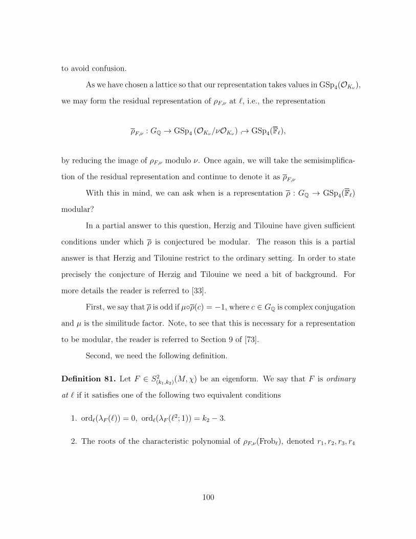
to avoid confusion.

As we have chosen a lattice so that our representation takes values in GSp4(OKν ),

we may form the residual representation of ρF,ν at `, i.e., the representation

ρF,ν : GQ → GSp4 (OKν/νOKν ) ↪→ GSp4(F`),

by reducing the image of ρF,ν modulo ν. Once again, we will take the semisimplifica-

tion of the residual representation and continue to denote it as ρF,ν

With this in mind, we can ask when is a representation ρ : GQ → GSp4(F`)

modular?

In a partial answer to this question, Herzig and Tilouine have given sufficient

conditions under which ρ is conjectured be modular. The reason this is a partial

answer is that Herzig and Tilouine restrict to the ordinary setting. In order to state

precisely the conjecture of Herzig and Tilouine we need a bit of background. For

more details the reader is referred to [33].

First, we say that ρ is odd if µ◦ρ(c) = −1, where c ∈ GQ is complex conjugation

and µ is the similitude factor. Note, to see that this is necessary for a representation

to be modular, the reader is referred to Section 9 of [73].

Second, we need the following definition.

Definition 81. Let F ∈ S2(k1,k2)(M,χ) be an eigenform. We say that F is ordinary

at ` if it satisfies one of the following two equivalent conditions

1. ord`(λF (`)) = 0, ord`(λF (`2; 1)) = k2 − 3.

2. The roots of the characteristic polynomial of ρF,ν(Frob`), denoted r1, r2, r3, r4

100

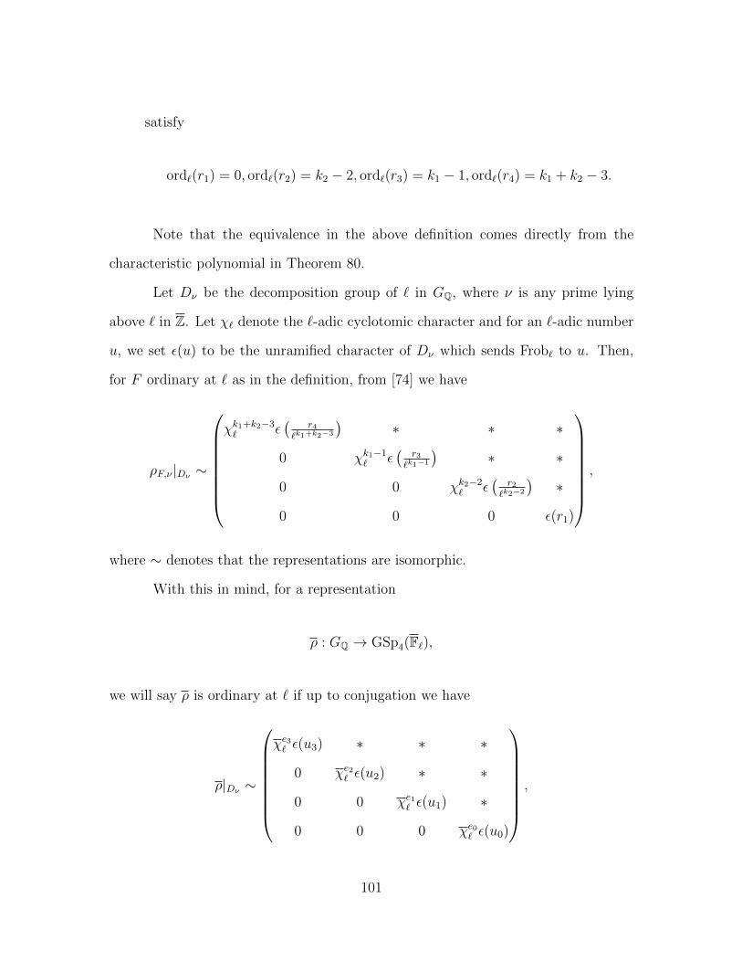
satisfy

ord`(r1) = 0, ord`(r2) = k2 − 2, ord`(r3) = k1 − 1, ord`(r4) = k1 + k2 − 3.

Note that the equivalence in the above definition comes directly from the

characteristic polynomial in Theorem 80.

Let Dν be the decomposition group of ` in GQ, where ν is any prime lying

above ` in Z. Let χ` denote the `-adic cyclotomic character and for an `-adic number

u, we set ε(u) to be the unramified character of Dν which sends Frob` to u. Then,

for F ordinary at ` as in the definition, from [74] we have

ρF,ν |Dν ∼

χk1+k2−3` ε

(r4

`k1+k2−3

)∗ ∗ ∗

0 χk1−1` ε

(r3

`k1−1

)∗ ∗

0 0 χk2−2` ε

(r2

`k2−2

)∗

0 0 0 ε(r1)

,

where ∼ denotes that the representations are isomorphic.

With this in mind, for a representation

ρ : GQ → GSp4(F`),

we will say ρ is ordinary at ` if up to conjugation we have

ρ|Dν ∼

χe3` ε(u3) ∗ ∗ ∗

0 χe2` ε(u2) ∗ ∗

0 0 χe1` ε(u1) ∗

0 0 0 χe0` ε(u0)

,

101

where χ` is the reduction of χ` modulo `, the exponents satisfy e3 ≥ e2 ≥ e1 ≥ e0, ε is

as above, and u3, u2, u1, u0 ∈ Fx

`. We denote such a representation as (ρ, {ej}). After

twisting by an appropriate power of χ` we may assume e0 = 0 and that ej ≤ j(`− 2)

for j = 1, 2, 3. This brings us to the next definition.

Definition 82. For a representation (ρ, {ej}), as above, we say that the exponents

{ej} are `-small if we can twist ρ by a power of χ` so that 0 = e0 ≤ e1 ≤ e2 ≤ e3 < `−1.

Furthermore, if we can write e1 = k2 − 2 and e2 = k1 − 1 for some integers

k1 ≥ k2 ≥ 3 then we call (k1, k2) the modular weight of (ρ, {ej}) .

We are now prepared to state the following conjecture.

Conjecture 83. [33, Conj. 0] Let (ρ, {ej}) be an irreducible, odd Galois represen-

tation which is ordinary at ` and has modular weight (k1, k2). Suppose further that

the exponents {ej} are `-small. Then, ρ is modular of level N with ` - N .

As evidence for this conjecture, we can state the following corollary which

follows from Theorem 55.

Corollary 84. Suppose that ρ is modular of level `rN and character χ of conductor

`N with ` - N . Then, ρ is modular of level N .

Proof. Suppose that ρ arises from F ∈ S(k1,k2)(`rN,χ). Then, we can apply Theorem

55 to obtain a representation ρ′ of level N such that the characteristic polynomials of

ρ(Frobp) and ρ′(Frobp) are equal for all p - `N . Thus, the characteristic polynomials

of ρ and ρ′ are equal everywhere by the Chebotarev Density Theorem. Just as in

the proof of Corollary 79, the Brauer-Nesbitt Theorem gives that ρ is isomorphic to

ρ′.

Finally, while the previous corollary made no restriction on the reducibility

of the Galois representations, we also have a slightly different level stripping result

102

which holds for certain reducible Galois representations. We remark that the reducible

representations in this setting have been classified in [66]. In particular, the reader is

referred to Section 3.2.

We will assume that the Galois representation

ρ : GQ → GL4(F`)

is modular and arises from a genus 2 Siegel modular form which appears as a Saito-

Kurokawa lift or a weak endoscopic lift. For our purposes, it is enough to note that

the Saito-Kurokawa lift provides a lifting of elliptic eigenforms to genus 2 Siegel eigen-

forms in which the associated Galois representation has a one-dimensional invariant

subspace, and the weak endoscopic lift provides a lifting from 2 elliptic eigenforms to

a genus 2 Siegel eigenform in which the associated Galois representation is reducible

but has no one dimensional invariant subspace.

As we gave the necessary facts for our purposes concerning the Saito-Kurokawa

lift in Section 4.7, we only need consider the weak endoscopic lifting here. Let f1 ∈

S1r1

(N,χ) and f2 ∈ S1r2

(N,χ) be normalized eigenforms with χ = ψ2 for some Dirichlet

character ψ defined modulo N . Let Ff1,f2 ∈ S2(k1,k2)(N,ψ) be a weak endoscopic lift

of f1 and f2. Then, for all primes p - N , the L-function of Ff1,f2 satisfies

Lp(s, Ff1,f2) = Lp(s, f1)Lp(s+ (r2 − r1)/2, f2),

where Lp(·) is the local L-factor defined in Chapter 2. Once again, we use this

103

factorization to deduce the following relationships

λFf1,f2 (p;S) = λf1(p) + pr1−r2

2 λf2(p),

λFf1,f2 (p2;S) = λf1(p)2 + pr1−r2λf2(p)

2 + pr1−r2

2 λf1(p)λf2(p)− χ(p2)pr1−2(2p+ 1),

(5.1)

for all primes p - N . For more details concerning the weak endoscopic lift, the reader

is referred to [77], [78], and [80]. Moreover, as a special case of the weak endoscopic

lift, there is the slightly better known Yoshida lift. The interested reader is referred

to [40] and [84] for more details. We are now prepared to state and give a proof of

the corresponding level stripping result for Galois representations associated to these

lifts.

Theorem 85. Let ρ : GQ → GL4(F`) be a modular Galois representation of level

`rN and character having trivial tame ramification. Assume ρ is associated to a form

arising from one of the two lifts discussed above Then, ρ is modular of level N and

also arises from a lifted form.

Before beginning the proof, we simply note the difference between the con-

dition on the character in Corollary 84 and the condition on the character in this

theorem. In Corollary 84, we have assumed that the character factored as ωiκ where

ω is the Teichmuller character, κ is a character defined modulo N , and i ∈ Z/(p−1)Z.

In the statement of Theorem 85, we are assuming that the character factors as ηκ

where η has conductor `α with α > 1 and κ is defined modulo N .

Proof. We provide the technique of the proof as the details are completely elementary.

Just as in Corollary 84, we can reduce the proof to a level stripping problem for

the associated modular forms. Say ρ arises from the lifted form F . Then, we consider

104

the elliptic modular form(s) from which F is lifted. Applying Theorem 36, we can

strip powers of ` from these form(s). Then, after lifting, we obtain the desired Siegel

modular form. The content of this proof revolves around using the relationships in

Equation 4.3 or Equation 5.1, depending on the lift in question, to show that the

eigenvalues are in fact congruent. This involves carefully keeping track of the weight

in the proof of Theorem 36. It is this congruence which provides the need for the

restriction on the character. See [14] for the details.

105

Chapter 6

Future work

In this chapter we mention some open problems related to generalizing our

result.

6.1 Twisting of Siegel modular forms

Let F be as in Theorem 55, except with corresponding character of conductor

N`r for any r > 1. Note that in Theorem 55 we required that r = 1. Is there a way to

construct an eigenform with corresponding character of conductor N` whose Fourier

coefficients are congruent to those of F away from the level?

An affirmative answer to this question would allow us to relax the restrictions

on the character of F in Theorem 55. In the proof of Theorem 36, we saw that

this was accomplished by twisting the original form by an appropriate character so

that the conductor of the character is lowered. However, this technique is for elliptic

modular forms, and the generalization of this twisting to the genus 2 setting is not

so easy due to the lack of a nice relationship between Fourier coefficients and Hecke

eigenvalues, and also due to the ambiguity arising from having “multiple” Fourier

106

expansions to consider.

For example, twists of classical Siegel modular forms have been investigated

in [5], [37], [47], and [48]. All of these results rely on twists of either the Fourier

expansion of F or the Fourier Jacobi expansion of F , which is quite analogous to the

twisting of elliptic modular forms. However, in all of these cases, the twisted modular

forms only transform with respect to some subgroup of the congruence subgroups

which we have considered up to this point. There seems to be no obvious way of

relaxing this restriction.

Finally, in the recent preprint [51], the authors have taken the approach of

investigating character twists from the representation theoretic perspective. In par-

ticular, they consider the properties of a character twist of an automorphic represen-

tation which contains a vector fixed by certain paramodular groups. In the sequel

to this work, the authors intend to translate this result to the more classical setting

of paramodular forms. It remains to be seen if such a twisting will translate to the

setting of Siegel modular forms.

6.2 Level stripping for reducible Galois represen-

tations

Let E is the Eisenstein series introduced in Section 4.2. If F is a Saito-

Kurokawa lift (respectively a weak endoscopic lift), then is the Deligne-Serre lift of

the form EF also a Saito-Kurokawa lift (respectively a weak endoscopic lift)?

An affirmative answer to this question would allow us to eliminate the char-

acter restriction in the statement of Theorem 85.

If we first consider the case that F is a Saito-Kurokawa lift, then this prob-

107

lem should be approachable by showing that the resulting form satisfies the Maass

relations on the Fourier-Jacobi coefficients. The correct Maass relations, however,

must be determined in the case of arbitrary level. Note, this is related to problem (3)

in [35]. We also mention an alternate approach to this problem which follows from

results in [26]. In this paper, the authors produce local criteria for determining when

a given Siegel modular form is a Saito-Kurokawa lift. The benefit being that these

criteria involve checking only finitely many conditions, as opposed to showing the

Maass relations hold. However, it is once again necessary to determine the correct

notion of these criteria for arbitrary level.

In the case that F arises as a weak endoscopic lift, it should be sufficient to

determine that the local factors of the spinor L-function associated to the Deligne-

Serre lift of FE factor appropriately for almost all factors. However, this sufficient

condition is only known for square-free level, as the results concerning weak endoscopic

lifts are primarily in the language of representation theory. Once again, the correction

conditions remain to be determined for arbitrary level.

6.3 Level stripping for arbitrary genus

Can we find an Eisenstein series of arbitrary genus analogous to the one used

in the proof of Theorem 55, i.e., can we find an Eisenstein series, E, of genus n, level

`, and character ω−i (as in the proof) such that E ≡fc 1 (mod `)?

Note that this is closely related to Problem 4.1 from [45]. If one could answer

this question affirmatively then we could generalize Theorem 55 to arbitrary genus.

Recently, in [41], the author was able to construct a `-adic Siegel modular form

of arbitrary genus, which interpolates the Fourier coefficients of the Siegel Eisenstein

series with prescribed character. This result was obtained using techniques from

108

Hida theory as it applies to Siegel modular forms. This construction naturally yields

a family of forms which are close `-adically. However, for this to be sufficient for

our purposes, one still requires a calculation of the `-adic valuation of the Fourier

coefficients as was done in [45] for the genus 2 setting. Given the explicit nature of

the construction in [41], this calculation should be tractable, though tedious.

6.4 Level stripping of automorphic representations

Finally, can one reproduce the proof of Theorem 55 in the language of auto-

morphic representations?

To be more precise about what this question means, we must first deal with the

most basic issue of how one reduces an automorphic representation modulo a prime.

This was introduced in a very general setting by Gross in [31]. Essentially, this is

accomplished by finding a lattice of the representation space which is stable under Z`

linear combinations of the Hecke operators. This allows one to extract an “integral”

model for the automorphic representation, which can then be reduced modulo `. At

the heart of this process, one must separate the infinite component from the finite

components of the automorphic representations and treat them separately. With this

in mind, one can try to reproduce the proof of Theorem 55 by calculating the effect

on the infinite and finite portion of the corresponding automorphic representations

separately.

The reason for desiring a result of this type is for purposes of generalization.

While arithmetic questions are typically more approachable in the classical language

of modular forms, these typically have a very limited scope as to how they apply

in other settings. By translating to the language of automorphic representations,

it is expected that a quite general framework for producing congruences will arise,

109

independent of the underlying group.

110

Appendices

111

Appendix A Explicit action of Hecke operators in

genus 2

In this section, we provide explicit formulas for the action of Hecke operators

on genus 2 Siegel modular forms. We will adapt techniques used by Andrianov in [4]

for scalar weight modular forms to the vector valued setting.

First, we derive a basic property of Fourier coefficients, which will help moti-

vate our technique. Let F ∈M2ρ (N,χ). As we have seen, the Fourier expansion of F

at ∞ is of the form

F (Z) =∑T∈Λ2

aF (T ) exp(Tr(TZ)) with aF (T ) ∈ V,

where ρ : GL2(C) → GL(V ). Furthermore, each Fourier coefficient is given by the

integral ∫X (mod 1)

F (Z) exp(−Tr(TZ))dX,

where we write Z = X+iY , dX is the Euclidean volume of the space of X coordinates,

and the integral runs over −1/2 ≤ Xij ≤ 1/2 for all i, j. This integral formula allows

us to derive the following relationship between the Fourier coefficients of F ,

aF (MT TM) =

∫X (mod 1)

F (Z) exp(−Tr(MT TMZ))dX

=

∫X (mod 1)

F (Z) exp(−Tr(T TMZM))dX

= χ(det(M))ρ(M)

∫X (mod 1)

F (TMZM) exp(−Tr(T TMZM))dX

= χ(det(M))ρ(M)aF (T ),

112

where M ∈ GL2(Z). Note, to move from the second line to the third line we use that

F (Z) = χ(det(M))ρ(M)F (TMZM),

which follows from the transformation property of F and noticing that

TM 0

0 M−1

∈ Γ20(N).

In summary, the desired property of the Fourier coefficients of F is

aF (MT TM) = χ(det(M))ρ(M)aF (T ), for all M ∈ GL2(Z). (1)

With this property in mind, we define a more general space of functions. Let

F(V ) denote the space of holomorphic functions F : h2 → V which have a Fourier

expansion of the form

F (Z) =∑T∈Λ2

aF (T ) exp(Tr(TZ)) with aF (T ) ∈ V.

Let ε be a character of the group GL2(Z). Define a subspace Fε(V ) ⊂ F(V ) by

considering only functions F ∈ F(V ) which satisfy

ε(M)F ((TMZ +M ′)M) = F (Z), for all

TM M ′

0 M−1

∈ P4,

where P4 is the Siegel parabolic subgroup. To summarize, we have defined the space

Fε(V ), to behave like modular forms with respect to the Siegel parabolic subgroup,

rather than congruence subgroups. Using an argument as in the preceding paragraph

113

we have that for F ∈ Fε(V ), the Fourier coefficients satisfy

aF (MT TM) = ε(M)aF (T ),

where M ∈ GL2(Z). Note that by Equation 1, we have that M2ρ (N,χ) ⊆ Fε(V ) if

ε(M) = χ(det(M))ρ(M). Throughout, we will fix a ρ, χ and set ε = χρ.

As our functions in Fε(V ) behave like modular forms with respect to the Siegel

parabolic subgroup, it makes sense to define the double coset operator in this setting

P4αP4 : Fε(V )→ Fε(V ),

given by

F [P4αP4]ε =∑i

χ(αi)F |εαi,

where we are summing over a complete set of coset representatives for P4\P4αP4,

α ∈ GSp+4 (Q) satisfies cα = 0, and the slash operator is defined to be (F |εγ)(Z) =

ρ(dγ)−1F (γZ).

In [4], Andrianov defines a map, ι, from HZ(Γ20(N)) to the double coset oper-

ators of the type listed above. This map is defined by

ι :∑i

Γ20(N)αi 7→

∑i

P4αi.

The benefit of this somewhat messy map can be seen in the following lemma, which

provides us with a compatibility between the Hecke operators on M2ρ (N,χ) and the

double coset operators on Fε(V ).

Lemma 86. Let F ∈M2ρ (N,χ). Then, TF = ι(T )F , for every T ∈ HZ(Γ2

0(N)).

Proof. Note, this is stated as part of Lemma 4.12 from [4], we simply restate it here to

114

emphasize that we are interested in vector valued modular forms, not just the scalar

valued case.

The lemma follows from the fact that we can find coset representatives, {αi}

for T which have cαi = 0 for all i.

With this lemma in mind, we use explicit coset representatives computed for

double cosets of the form P4\P4αP4 to compute formulas for the action of elements of

HZ(Γ20(N)). In fact, it is enough for our purposes to give coset representatives for ι

applied to the generators of HZp (Γ2

0(N)) taken from Theorem 25 for each p - N . First,

we give the image of these generators as double cosets, then we will give their explicit

decompositions.

Lemma 87. [4, Lemma 3.64]

ι(T (p)) = [P4 diag(p, p, 1, 1)P4] + [P4 diag(p, 1, 1, p)P4] + [P4 diag(1, 1, p, p)P4],

ι(T1(p2)) =1

p[P4 diag(p, p, 1, 1)P4][P4 diag(p, 1, 1, p)P4]

+1

p[P4 diag(p, 1, 1, p)P4][P4 diag(1, 1, p, p)P4]

+1

p[P4 diag(p, 1, 1, p)P4]2 − [P4 diag(p2, 1, 1, p2)P4]

− p+ 1

p3[P4 diag(p, p, 1, 1)P4][P4 diag(1, 1, p, p)P4],

ι(T2(p2)) =1

p3[P4 diag(p, p, 1, 1)P4][P4 diag(1, 1, p, p)P4].

Combining Lemma 3.60 and Proposition 3.61 from [4], we obtain the following

left coset decompositions for the double coset operators in the previous lemma,

P4\P4 diag(p, p, 1, 1)P4 = P4

pI2 02

02 I2

,

115

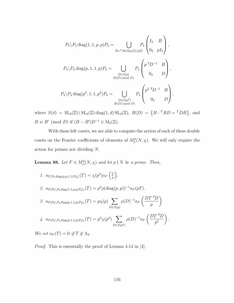
P4\P4 diag(1, 1, p, p)P4 =⋃

B=TB∈M2(Z)/pZ)

P4

I2 B

02 pI2

,

P4\P4 diag(p, 1, 1, p)P4 =⋃

D∈S(p)B(D) (mod D)

P4

p TD−1 B

02 D

,

P4\P4 diag(p2, 1, 1, p2)P4 =⋃

D∈S(p2)B(D) (mod D)

P4

p2 TD−1 B

02 D

,

where S(d) = SL2(Z)\ SL2(Z) diag(1, d) SL2(Z), B(D) ={B : TBD = TDB

}, and

B ≡ B′ (mod D) if (B −B′)D−1 ∈ M2(Z).

With these left cosets, we are able to compute the action of each of these double

cosets on the Fourier coefficients of elements of M2ρ (N,χ). We will only require the

action for primes not dividing N .

Lemma 88. Let F ∈M2ρ (N,χ) and let p - N be a prime. Then,

1. aF [P4 diag(p,p,1,1)P4]ε(T ) = χ(p2)aF

(Tp

).

2. aF [P4\P4 diag(1,1,p,p)P4]ε(T ) = p3ρ(diag(p, p))−1aF (pT ).

3. aF [P4\P4 diag(p,1,1,p)P4]ε(T ) = pχ(p)∑

D∈S(p)

ρ(D)−1aF

(DT TD

p

)

4. aF [P4\P4 diag(p,1,1,p)P4]ε(T ) = p2χ(p2)∑

D∈S(p2)

ρ(D)−1aF

(DT TD

p2

).

We set aF (T ) = 0 if T 6∈ Λ2.

Proof. This is essentially the proof of Lemma 4.14 in [4].

116

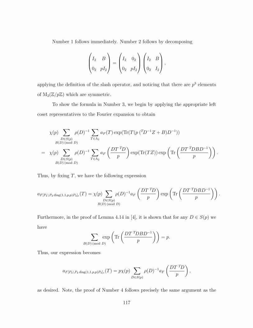
Number 1 follows immediately. Number 2 follows by decomposing

I2 B

02 pI2

=

I2 02

02 pI2

I2 B

02 I2

,

applying the definition of the slash operator, and noticing that there are p3 elements

of M2(Z/pZ) which are symmetric.

To show the formula in Number 3, we begin by applying the appropriate left

coset representatives to the Fourier expansion to obtain

χ(p)∑

D∈S(p)B(D) (mod D)

ρ(D)−1∑T∈Λ2

aF (T ) exp(Tr(T (p (TD−1Z +B)D−1))

= χ(p)∑

D∈S(p)B(D) (mod D)

ρ(D)−1∑T∈Λ2

aF

(DT TD

p

)exp(Tr(TZ)) exp

(Tr

(DT TDBD−1

p

)).

Thus, by fixing T , we have the following expression

aF [P4\P4 diag(1,1,p,p)P4]ε(T ) = χ(p)∑

D∈S(p)B(D) (mod D)

ρ(D)−1aF

(DT TD

p

)exp

(Tr

(DT TDBD−1

p

)).

Furthermore, in the proof of Lemma 4.14 in [4], it is shown that for any D ∈ S(p) we

have ∑B(D) (mod D)

exp

(Tr

(DT TDBD−1

p

))= p.

Thus, our expression becomes

aF [P4\P4 diag(1,1,p,p)P4]ε(T ) = pχ(p)∑

D∈S(p)

ρ(D)−1aF

(DT TD

p

),

as desired. Note, the proof of Number 4 follows precisely the same argument as the

117

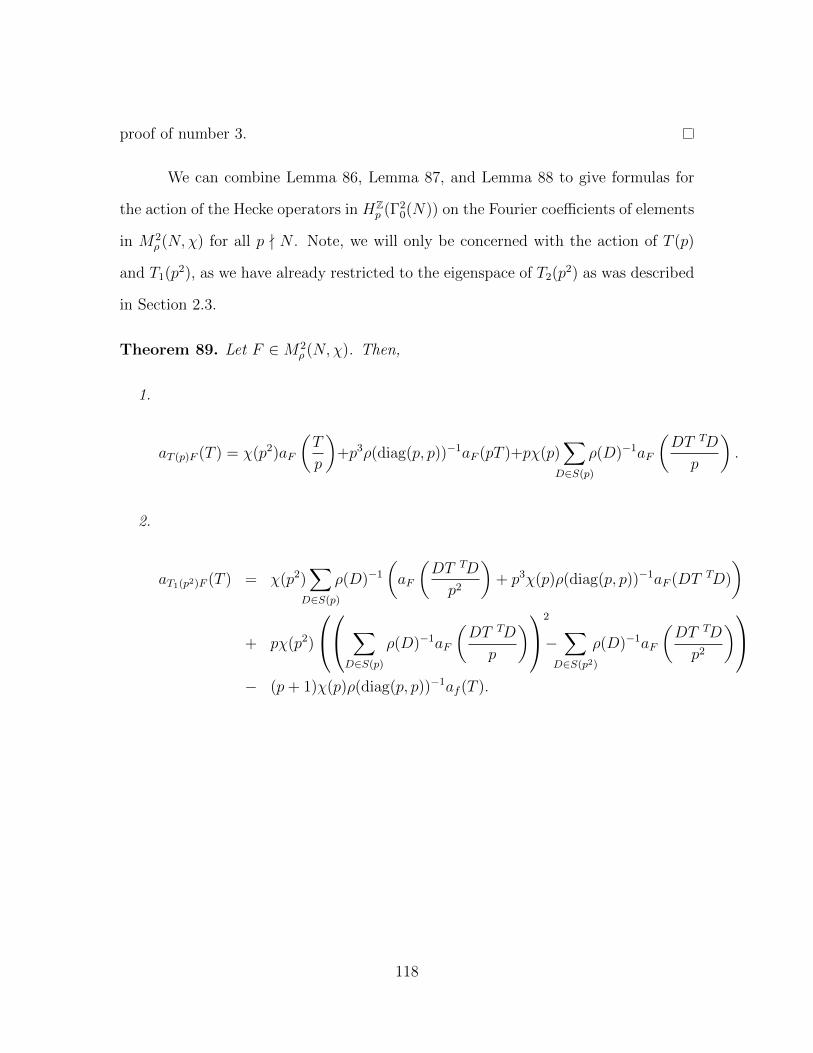
proof of number 3.

We can combine Lemma 86, Lemma 87, and Lemma 88 to give formulas for

the action of the Hecke operators in HZp (Γ2

0(N)) on the Fourier coefficients of elements

in M2ρ (N,χ) for all p - N . Note, we will only be concerned with the action of T (p)

and T1(p2), as we have already restricted to the eigenspace of T2(p2) as was described

in Section 2.3.

Theorem 89. Let F ∈M2ρ (N,χ). Then,

1.

aT (p)F (T ) = χ(p2)aF

(T

p

)+p3ρ(diag(p, p))−1aF (pT )+pχ(p)

∑D∈S(p)

ρ(D)−1aF

(DT TD

p

).

2.

aT1(p2)F (T ) = χ(p2)∑

D∈S(p)

ρ(D)−1

(aF

(DT TD

p2

)+ p3χ(p)ρ(diag(p, p))−1aF (DT TD)

)

+ pχ(p2)

∑D∈S(p)

ρ(D)−1aF

(DT TD

p

)2

−∑

D∈S(p2)

ρ(D)−1aF

(DT TD

p2

)− (p+ 1)χ(p)ρ(diag(p, p))−1af (T ).

118

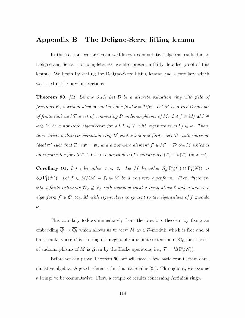
Appendix B The Deligne-Serre lifting lemma

In this section, we present a well-known commutative algebra result due to

Deligne and Serre. For completeness, we also present a fairly detailed proof of this

lemma. We begin by stating the Deligne-Serre lifting lemma and a corollary which

was used in the previous sections.

Theorem 90. [21, Lemme 6.11] Let D be a discrete valuation ring with field of

fractions K, maximal ideal m, and residue field k = D/m. Let M be a free D-module

of finite rank and T a set of commuting D endomorphisms of M . Let f ∈M/mM ∼=

k ⊗M be a non-zero eigenvector for all T ∈ T with eigenvalues a(T ) ∈ k. Then,

there exists a discrete valuation ring D′ containing and finite over D, with maximal

ideal m′ such that D ∩m′ = m, and a non-zero element f ′ ∈M ′ = D′ ⊗DM which is

an eigenvector for all T ∈ T with eigenvalue a′(T ) satisfying a′(T ) ≡ a(T ) (mod m′).

Corollary 91. Let i be either 1 or 2. Let M be either Siρ(Γi0(`r) ∩ Γi1(N)) or

Sρ(Γi1(N)). Let f ∈ M/`M = F` ⊗ M be a non-zero eigenform. Then, there ex-

ists a finite extension Oν ⊇ Z` with maximal ideal ν lying above ` and a non-zero

eigenform f ′ ∈ Oν ⊗Z` M with eigenvalues congruent to the eigenvalues of f modulo

ν.

This corollary follows immediately from the previous theorem by fixing an

embedding Q ↪→ Q` which allows us to view M as a D-module which is free and of

finite rank, where D is the ring of integers of some finite extension of Q`, and the set

of endomorphisms of M is given by the Hecke operators, i.e., T = H(Γi0(N)).

Before we can prove Theorem 90, we will need a few basic results from com-

mutative algebra. A good reference for this material is [25]. Throughout, we assume

all rings to be commutative. First, a couple of results concerning Artinian rings.

119

Lemma 92. If R is an Artinian integral domain, then R is a field.

Proof. Let x ∈ R be non-zero and consider the descending chain of ideals

(x) ⊇ (x2) ⊇ · · · .

As this chain eventually stabilizes, we have xn = axn+1 for some positive integer n

and some a ∈ R. As R is an integral domain, we conclude that x is a unit, and hence

R is a field.

Corollary 93. Any prime ideal of an Artinian ring is maximal.

Proof. Let R be an Artinian ring and ℘ ⊆ R be a prime ideal. Then, R/℘ is an

Artinian integral domain, and, by the previous lemma, a field.

Next, we will need a few results concerning associated primes, which we first

define.

Definition 94. Let R be a ring and M an R-module. A prime ideal ℘ ⊂ R is said

to be associated to M if ℘ is the annihilator of an element of M .

Lemma 95. Let M be an R-module. Then, the set of prime ideals of R which are

associated primes of M is contained in the set of prime ideals of R which are in the

support of M .

Proof. Let ℘ be an associated prime of M . Then, ℘ is the annihilator of some m ∈M .

If the localization of M at ℘, denoted M℘, is zero, then there exists x ∈ R − ℘ such

that xm = 0. This implies that x ∈ ℘, which is a contradiction. Thus, M℘ 6= 0, i.e.,

℘ is a support prime of M .

Lemma 96. Let R be a Noetherian ring, M a non-zero R-module, and ℘ a prime in

the support of M . Then, ℘ contains an associated prime of M .

120

Proof. Since ℘ is in the support of M , there is some x ∈ M satisfying (Rx)℘ 6= 0.

Since R is Noetherian, Theorem 3.1 in [25] gives that the set of associated primes of

(Rx)℘ is non-empty. The previous lemma gives that the associated primes of (Rx)℘

is contained in the support of (Rx)℘. Let p be an associated prime of (Rx)℘. Then,

there is a non-zero element x′

y∈ (Rx)℘ with x′ ∈ Rx and y ∈ R − ℘, such that p is

the annihilator of x′

y.

Suppose z ∈ p− ℘. Then, z x′

y= 0, which implies that x′

y= 0 since z is a unit

in (Rx)℘. Hence, no such z exists, i.e., p ⊆ ℘.

As R is Noetherian, we have that any p is finitely generated. Let {z1, . . . , zn}

be a set of generators for p. Then, for each zi, there exists a ti ∈ R − ℘ such that

zitix′ = 0. Let t = t1 . . . tn. Then, p is the annihilator of tx′ ∈ M . Thus, p is an

associated prime of M .

With these results in hand, we are prepared to prove the main result of this

section.

Proof of Theorem 90. Let H be the D-subalgebra of EndD(M) generated by T over

D. Since M is free and of rank r < ∞ over D, we have that EndD(M) is a free

D-module of rank r2. Hence, H is free and of finite rank. Choosing a basis for H,

we may assume T = {T1, T2, . . . , Tn} is a finite set. It will be sufficient to prove the

theorem for these basis elements.

Let mTi be the minimal polynomial of Ti. By adjoining all roots of mTi to K

for all i, we have a finite field extension K ⊆ K ′ such that each mTi splits over K ′.

The integral closure of D in K ′ gives a discrete valuation ring D′ with maximal ideal

m′ satisfying D ∩ m′ = m, and residue field k′ containing k. Furthermore, we have

that D′⊗DM is a D′ module, and we will continue to denote this module by M , and

we will also continue to denote the analogous subalgebra of endomorphisms, D′⊗DH,

121

by H.

Consider the homomorphism of D′-algebras,

πf : H → k′, given by πf (T ) = a(T ) (mod m′).

Note, we have an obvious injection of D′ into H, which implies that πf is surjective.

By Zorn’s lemma, we can choose a minimal non-zero prime ideal p ⊂ H which is

contained in the maximal ideal kerπf .

Claim. The prime ideal p is contained in the set of zero divisors of H.

Proof of Claim. Let Z denote the set of zero divisors of H. Let D = H − Z. Note,

D is closed under multiplication.

Consider the set S = H − p. As p is prime, we have that S is closed under

multiplication. Furthermore, if S ′ is a multiplicatively closed set which contains S,

then S ′ = H or S ′ = H − p′ for some prime ideal p′ ⊂ p. As p is minimial, we

must have S ′ = H, and hence S is a maximal multiplicatively closed set. If D is not

contained in S, then SD is a multiplicatively closed set strictly containing S, i.e.,

SD = H, which is impossible since 0 /∈ SD. Thus, D ⊂ S, which implies p ⊂ Z.

The fact that H is free over D′ and D′ is an integral domain combined with

the previous claim gives that p ∩ D′ = 0, where we are again considering D′ as lying

in H. Further, note that as H is finitely generated over D′, so is H/pH, hence H/pH

is a finite integral extension of D′. Let L be the field of fractions of H/pH, and let

DL denote the integral closure of D′ in L, with mL the corresponding maximal ideal

and l the corresponding residue field.

122

Consider the projection

π′f : H → H/pH ↪→ DL,

where the final injection comes from the fact that H/pH is an integral extension of

D′ and DL is the integral closure of D′ in L. Recall, for πf defined above, we have

that ker πf is a maximal ideal in H. Combining Proposition 4.15 and Corollary 4.17

in [25], we have that π′f (kerπf ) ⊆ mL.

Let π′f (T ) = a′(T ) ∈ H/pH ⊂ DL, for all T ∈ H. Then,

πf (T − a(T )I) = πf (T )− a(T )πf (1) = a(T )− a(T ) = 0,

i.e., T − a(T ) ∈ kerπf . It follows that π′f (T − a(T )I) = a′(T ) − a(T ) ∈ mL, i.e.,

a′(T ) ≡ a(T ) (mod mL).

Let p′ be the prime ideal in K ′ ⊗D′ H which is generated by p. Since p is

minimal, so is p′. We want to show that p′ is an associated prime of K ′ ⊗D′ M ,

i.e., that p′ is the annihilator of some nonzero element of K ′ ⊗D′ M . As our tensor

products will be over D′ for the remainder of the proof, we will drop this from the

notation.

First, we need that K ′⊗H is Artinian and has all maximal ideals isomorphic.

This follows simply from the fact that H is free and of finite rank over D′, which

implies that

K ′ ⊗H ∼=n⊕i=1

K ′,

for some n < ∞. It is clear that all maximal ideals of⊕n

i=1 K′ are isomorphic.

Furthermore,⊕n

i=1 K′ is Artinian since K ′ is.

Note, the annihilator of K ′ ⊗M in K ′ ⊗ H, denoted AnnK′⊗H(K ′ ⊗M), is

123

an ideal in K ′ ⊗ H, and is hence is contained in some maximal ideal. By Corollary

93, we have that p′ is maximal in K ′ ⊗ H, and since all maximal ideals of K ′ ⊗ H

are isomorphic, we may assume that AnnK′⊗H(K ′ ⊗M) ⊂ p′. By Corollary 2.7 in

[25], we have that p′ is in the support of K ′⊗M , which gives that p′ is an associated

prime of K ′ ⊗M by Lemma 96 and the minimality of p′.

Thus, there is some f ′ ∈ K ′ ⊗M , which is annihilated by p′. Note, we may

assume that f ′ ∈ M by simply clearing denominators. As T − a′(T ) ∈ p′, we have

that Tf ′ = a′(T )f ′, and as we have already shown that a′(T ) ≡ a(T ) (mod mL), the

proof is complete.

124

Bibliography

[1] A. Andrianov. Quadratic forms and Hecke operators, volume 286 of GrundlehrenMath. Wiss. Springer-Verlag, 1987.

[2] A. Andrianov. On functional equations satisfied by spinor Euler products forSiegel modular forms of genus 2 with characters. Abh. Math. Sem. Univ. Ham-burg, 71:123–142, 2001.

[3] A. Andrianov. On diagonalization of singular frobenius operators on Siegel mod-ular forms. Amer. J. Math., 125:139–165, 2003.

[4] A. Andrianov. Introduction to Siegel modular forms and Dirichlet series. Uni-versitext. Springer, New York, NY, 2009.

[5] A. Andrianov. Twisting of Siegel modular forms with characters, and L-functions. St. Petersburg Math. J., 20(6):851–871, 2009.

[6] T. Arakawa. Vector values Siegel’s modular forms of degree two and the associ-ated Andrianov l-functions. Manuscripta Math., 44:155–186, 1983.

[7] S. Bocherer. On the Hecke operator U(p). J. Math. Kyoto Univ., 45-4:807–829,2005.

[8] S. Bocherer, J. Funke, and R. Schulze-Pillot. Trace operator and theta series. J.Number Theory, 78:119–139, 1999.

[9] S. Bocherer and S. Nagaoka. On p-adic properties of Siegel modular forms.Preprint.

[10] S. Bocherer and S. Nagaoka. On mod p properties of Siegel modular forms. Math.Ann., 338:421–433, 2006.

[11] S. Bocherer and S. Nagaoka. On Siegel modular forms of level p and theirproperties mod p. Manuscripta Math., 132:501–515, 2010.

[12] A. Borel. Linear algebraic groups, volume 126 of Graduate Texts in Mathematics.Springer-Verlag New York, 1991.

125

[13] C. Breuil, B. Conrad, F. Diamond, and R. Taylor. On the modularity of ellipticcurves over Q: wild 3-adic exercises. J. Amer. Math. Soc., 14:843–939, 2001.

[14] J. Brown and R. Keaton. Level stripping for Siegel modular forms with reducibleGalois representations. J. Number Theory, 133(5):1492–1501, 2013.

[15] D. Bump. Automorphic Forms and Representations, volume 55 of CambridgeStudies in Advanced Mathematics. Cambridge University Press, 1998.

[16] K. Buzzard. On level-lowering for mod 2 representations. Math. Res. Lett.,7(1):96–110, 2000.

[17] I. Chen, I. Kiming, and J. Rasmussen. On the congruences mod pm be-tween eigenforms and their attached Galois representations. J. Number Theory,130:608–619, 2010.

[18] R. Coleman and J.-F. Voloch. Companion forms and Kodaira-Spencer theory.Invent. Math., 110:263–282, 1992.

[19] J. Conway and N. Sloane. Sphere packings, lattices, and groups, volume 290 ofA series of comprehensive studies in mathematics. Springer-Verlag, 1999.

[20] P. Deligne. Formes modulaires et representations `-adiques. Ann. scient. Ec.Norm. Sup., 7:507–530, 1974.

[21] P. Deligne and J-P. Serre. Formes modulaires de poids 1. Ann. scient. Ec. Norm.Sup., 7:507–530, 1974.

[22] F. Diamond. The refined conjecture of Serre. In J. Coates and S.-T. Yau, editors,Elliptic Curves and Fermat’s Last Theorem, pages 172–186. International Press,1997.

[23] F. Diamond and J. Shurman. A First Course in Modular Forms, volume 228 ofGraduate Texts in Mathematics. Springer, 2005.

[24] M. Eichler and D. Zagier. The Theory of Jacobi Forms, volume 55 of Progressin Mathematics. Birkhauser, 1985.

[25] D. Eisenbud. Commutative Algebra With a View Toward Algebraic Geometry,volume 150 of Graduate Texts in Mathematics. Springer-Verlag, 1995.

[26] A. Ryan N. Schmidt R. Farmer, D. Pitale. Survey article: Characterizations ofthe Saito-Kurokawa lifting. Rocky Mountain J. Math., 43:1747–2083, 2013.

[27] E. Freitag. Singular modular forms and theta relations. Lecture Notes in Math-ematics, 1487:419–440, 1991.

126

[28] W. Fulton and J. Harris. Representation theory: A first course, volume 129 ofGraduate Texts in Mathematics. Springer-Verlag, 1991.

[29] D. Goldfeld and J. Hundley. Automorphic Representations and L-Functionsfor the General Linear Group, volume 129 of Cambridge Studies in AdvancedMathematics. Cambridge University Press, 2011.

[30] B. Gross. A tameness criterion for Galois representations associated to modularforms (mod p). Duke Math. J., 61:445–516, 1990.

[31] B. Gross. Algebraic modular forms. Israel J. Math., 113:61–93, 1999.

[32] J. Hafner and L. Walling. Siegel modular forms and Hecke operators in degree2. Millennial Conference on Number Theory, 2002.

[33] F. Herzig and J. Tilouine. Conjecture de type de Serre et formes compagnonspour GSp4. J. Reine Angew. Math., 676:1–32, 2013.

[34] H. Hida. Elementary Theory of L-functions and Eisenstein series, volume 26of London Mathematical Society Student Texts. Cambridge University Press,Cambridge, 1993.

[35] T. Ibukiyama. Saito-Kurokawa liftings of level N and practical construction ofJacobi forms. Kyoto J. Math., 52(1):141–178, 2012.

[36] T. Ichikawa. Vector valued p-adic Siegel modular forms. J. reine angew. Math.,to appear.

[37] O. Imamoglu and Y. Martin. On characteristic twists of multiple Dirichlet seriesassociated to Siegel cusp forms. Math. Zeitschrift, 263:345–368, 2009.

[38] K. Ireland and M. Rosen. A Classical Introduction to Modern Number Theory,volume 84 of Graduate Texts in Mathematics. Springer-Verlag New York, 1990.

[39] K. Iwasawa. Lectures on p-adic L-functions. Princeton University Press, 1972.

[40] J. Jia. Arithmetic of the Yoshida lift. PhD thesis, University of Michigan, AnnArbor, 2010.

[41] H. Kawamura. A semi-ordinary p-stabilization of Siegel Eisenstein series forsymplectic groups and its p-adic interpolation. arXiv:1207.0198v3.

[42] R. Keaton. Level stripping for degree 2 Siegel modular forms. Math. Res. Lett.,20(5):919–932, 2013.

[43] C. Khare and J-P. Wintenberger. Serre’s modularity conjecture (I). Invent.Math., 178:485–504, 2009.

127

[44] C. Khare and J-P. Wintenberger. Serre’s modularity conjecture (II). Invent.Math., 178:505–586, 2009.

[45] T. Kikuta. On p-adic Siegel modular forms of non-real nebentypus of degree 2.Acta Arith., 152:175–183, 2012.

[46] N. Koblitz. Introduction to Elliptic Curves and Modular Forms, volume 97 ofGraduate Texts in Mathematics. Springer-Verlag New York, 1984.

[47] W. Kohnen. On characteristic twists of certain Dirichlet series. Mem. Fac. Sci.Kyushu Univ. Ser. A, 47(1):103–117, 1993.

[48] W. Kohnen, A. Krieg, and J. Sengupta. Characteristic twists of a Dirichlet seriesfor Siegel cusp forms. Manusc Math., 87:489–499, 1995.

[49] N. Kurokawa. On Siegel eigenforms. Proc. Japan Acad. Ser. A, 57:47–50, 1981.

[50] G. Laumon. Fonctions zeta des varietes de Siegel de dimension trois. Asterisque,302:1–66, 2005.

[51] J. Leung-Johnson and B. Roberts. Twisting of paramodular vectors. Int. J.Number Theory, pages 1–23.

[52] W. Li. Newforms and functional equations. Math. Ann., 212:285–315, 1975.

[53] M. Manickam and B. Ramakrishnan. On Shimura, Shintani and Eichler-Zagiercorrespondences. Trans. Amer. Math. Soc., 352:2601–2617, 2000.

[54] M. Manickam and B. Ramakrishnan. On Saito-Kurokawa correspondence ofdegree two for arbitrary level. J. Ram. Math. Soc., 17(3):149–160, 2002.

[55] T. Miyake. Modular Forms. Springer-Verlag Berlin Heidelberg, 1989.

[56] S. Mizumoto. Congruences for Fourier coefficients of lifted Siegel modular formsI: Eisenstein lifts. Abh. Math. Sem. Univ. Hamburg, 75:97–120, 2005.

[57] J. Neukirch. Algebraic Number Theory. Springer-Verlag Berlin Heidelberg, 1999.

[58] I. Piatetski-Shapiro. On the Saito-Kurokawa lifting. Invent. Math., 71:309–338,1983.

[59] K. Ribet. On modular representations of Gal(Q/Q) arising from modular forms.Invent. Math., 100:431–476, 1990.

[60] K. Ribet. Report on mod ` representations of Gal(Q/Q). In Motives, volume 55of Proc. Sympos. Pure. Math, pages 639–676, Providence, RI, 1994. Amer. Math.Soc.

128

[61] N. Ryan and T. Shemanske. Inverting the Satake map for Spn and applicationsto Hecke operators. Ramanujan J., pages 219–244, 2008.

[62] J-P. Serre. Proprietes galoisiennes des points d’ordre fini des courbes elliptiques.Invent. Math., 15:259–331, 1972.

[63] J-P. Serre. Formes modulaires et fonctions zeta p-adiques. Lecture Notes inMathematics, 350:191–268, 1973.

[64] J-P. Serre. Sur les representations modulaires de degre 2 de Gal(Q/Q). DukeMath. J., 54(1):179–230, 1987.

[65] G. Shimura. Introduction to the Arithmetic Theory of Automorphic Forms.Princeton University Press, 1971.

[66] C. Skinner and E. Urban. Sur les deformations p-adiques de certain representa-tions automorphes. J. Inst. Math. Jussieu, 5:629–698, 2006.

[67] J. Sturm. On the congruence of modular forms. Lecture Notes in Mathematics,1240:275–280, 1980.

[68] H. Takayanagi. Vector valued Siegel modular forms and their L-functions; Ap-plication of a differential operator. Japan J. Math., 19:251–297, 1994.

[69] Y. Takei. On algebraicity of vector valued Siegel modular forms. Kodai Math.J., 15:445–457, 1992.

[70] J. Tate. Fourier analysis in number fields, and Hecke’s zeta-functions. PhDthesis, Harvard University, 1950.

[71] R. Taylor. On Congruences Between Modular Forms. PhD thesis, PrincetonUniversity, 1988.

[72] R. Taylor and A. Wiles. Ring-theoretic properties of certain Hecke algebras.Ann. Math., 141:553–572, 1995.

[73] J. Tilouine. Deformations of Galois representations and Hecke algebras. NarosaPublishing House, 1996.

[74] E. Urban. Sur les representations p-adiques associees aux representations cuspi-dales de gsp4(Q). Asterisque, 302:151–176, 2005.

[75] G. van der Geer. Siegel modular forms and their applications. In 1-2-3 of ModularForms, Lectures at a Summer School in Nordfjordeid, Norway, pages 181–246.Universitext, 2008.

[76] L. Washington. Introduction to Cyclotomic Fields, volume 83 of Graduate Textsin Mathematics. Springer-Verlag New York, 1982.

129

[77] R. Weissauer. Preprints on the Ramanujan conjecture for GSp(4).http://www.mathi.uni-heidelberg.de/∼weissaue/papers/ramanuge.dvi, 1993/95.

[78] R. Weissauer. Four dimensional Galois representations. Asterisque, 302:67–150,2005.

[79] R. Weissauer. Existence of Whittaker models related to four dimensional sym-plectic Galois representations. In Modular Forms on Schiermonnikoog, pages285–310. Cambridge Univ. Press, 2008.

[80] R. Weissauer. Endoscopy for GSp(4) and Siegel modular threefolds, volume 1968of Lecture Notes in Mathematics. Springer-Verlag Berlin Heidelberg, 2009.

[81] M. Weissman. Multiplying modular forms. Preprint, 2007.

[82] G. Wiese. Galois representations. http://math.uni.lu/~wiese/notes/

GalRep.pdf, 2008.

[83] A. Wiles. Modular elliptic curves and Fermat’s last theorem. Ann. of Math.,141(3):443–551, 1995.

[84] H. Yoshida. Siegel’s modular forms and the arithmetic of quadratic forms. Invent.Math., 60(3):193–248, 1980.

[85] D. Zagier. Elliptic modular forms and their applications. In 1-2-3 of ModularForms, Lectures at a Summer School in Nordfjordeid, Norway, pages 1–103.Universitext, 2008.

130