Embed Size (px)
Citation preview

Document: PO-TN-IMK-GS-0003
ESA-Contract No. 11717/95/NL/CN
ESA-Contract No. 12078/96/NL/GS
Technical Note
Level 0 to 1b Data Processing of the MIPAS-B2
balloon borne Fourier Transform Spectrometer
Revision 1.2 of 17.05.2000
by O. Trieschmann
with inputs from F. Friedl-Vallon, A. Kleinert, A. Lengel, G. Wetzel
approved by H. Oelhaf
Forschungszentrum Karlsruhe
Institut für Meteorologie and Klimaforschung
P.O. Box 3640
D-76021 Karlsruhe

Page 2 of 100
History: Draft Version – February 1998 Revision 1 – 03.04.2000 Added: - Updated algorithm description - Description of ILS determination - Description of the level 1b parametrization - ILS-parametrisation Revision 1.1 – 17.04.2000 Comments by H. Nett are considered in subsections 6.5.1, 6.6, 7.3.1, 7.5.1, 7.5.3 and 8.2. Revision 1.2 – 17.05.2000 Updated subsection 7.5.3.

Page 3 of 100
1. Table of contents
1. Table of contents ................................................................................................... 3
2. Introduction............................................................................................................ 5
3. Typical measuring scenarios................................................................................ 7
4. Definition of the data levels .................................................................................. 9
5. Description of the processing chain .................................................................. 10
6. Overview of the processing algorithms of MIPAS-B2 ...................................... 13
6.1. Differences between MIPAS-B2 and MIPAS/ENVISAT data processing ....... 13 6.2. Phase correction of interferograms ................................................................ 14
6.2.1. Methods for phase determination and correction for MIPAS-B2 .............. 15 6.2.2. Results..................................................................................................... 20
6.3. Spectral and Radiometric Calibration............................................................. 21 6.4. Localisation .................................................................................................... 22 6.5. ILS determination ........................................................................................... 22
6.5.1. ILS parameterization................................................................................ 25
7. The parameterization of the individual processes............................................ 27
7.1. Interferogram processing independent of the source ..................................... 27 7.1.1. Interferogram check ................................................................................. 27 7.1.2. Interferogram non-linearity correction ...................................................... 27
7.2. Blackbody spectra.......................................................................................... 28 7.2.1. Phase determination of blackbody interferograms ................................... 28 7.2.2. Interferogram phase correction................................................................ 29 7.2.3. Generation of blackbody spectra ............................................................. 29 7.2.4. Co-addition of blackbody spectra............................................................. 30 7.2.5. Noise reduction in blackbody spectra (only channel 3) ............................ 30
7.3. Deep-space spectra ....................................................................................... 31 7.3.1. Co-addition of deep-space interferograms............................................... 31 7.3.2. Phase determination of deep-space spectra............................................ 32 7.3.3. Phase correction of deep-space interferograms ...................................... 32 7.3.4. Generation of deep-space spectra........................................................... 33 7.3.5. Shaving of deep-space spectra................................................................ 33
7.4. Limb sequence spectra .................................................................................. 33 7.4.1. Phase determination of limb sequence spectra ....................................... 33 7.4.2. Phase correction of limb sequence interferograms .................................. 33 7.4.3. Generation of limb sequence spectra ...................................................... 34
7.5. Calibration ...................................................................................................... 34 7.5.1. Radiometric calibration of limb spectra .................................................... 34 7.5.2. Interpolation on the ENVISAT spectral grid and spectral calibration........ 35 7.5.3. Calculation of variance of single consecutive spectra.............................. 36
8. Algorithms - Reference ....................................................................................... 37

Page 4 of 100
8.1. Apodisation functions ..................................................................................... 38 8.2. Co-addition of interferograms......................................................................... 41 8.3. Co-addition of spectra .................................................................................... 46 8.4. Conditioning of data sets for FFT ................................................................... 49 8.5. Convolution of data sets using FFT................................................................ 51 8.6. Fitting procedure with weighting coefficients .................................................. 52 8.7. Generation of spectra..................................................................................... 53 8.8. Generation of the variance of single consecutive spectra .............................. 56 8.9. Interferogram correction and mathematical filtering ....................................... 59 8.10. Kernel generation........................................................................................... 61 8.11. Phase determination ...................................................................................... 63
8.11.1. ‘Classical’ phase determination................................................................ 64 8.11.2. Differential Phase determination.............................................................. 67 8.11.3. Statistical phase determination ................................................................ 71
8.12. Radiometric calibration of the spectra ............................................................ 77 8.13. ‘Shaving’ - Removal of residual atmospheric lines in deep space spectra ..... 80
9. References ........................................................................................................... 85
10. Appendix .............................................................................................................. 88
10.1. Abbreviation and Notation .............................................................................. 88 10.2. List of wavenumbers of critical radiometric calibration ................................... 89
10.2.1. Channel 1 ................................................................................................ 89 10.2.2. Channel 2 ................................................................................................ 90 10.2.3. Channel 3 ................................................................................................ 91
10.3. Data exchange for MIPAS-B balloon data between IMK and IROE/Univ. of Bologna.......................................................................................................... 92
10.3.1. Purpose ................................................................................................... 92 10.3.2. Abbreviations ........................................................................................... 92 10.3.3. Definitions and general information.......................................................... 92 10.3.4. File formats .............................................................................................. 92 10.3.4.1. Channel descriptive data sets (ESA-Contract No. 11717/95/NL/CN and
ESA-Contract No. 12078/96/NL/GS)........................................................ 93 10.3.4.2. Spectral data sets (ESA-Contract No. 11717/95/NL/CN)......................... 94 10.3.4.3. Spectral data sets (ESA-Contract No. 12078/96/NL/GS)......................... 95 10.3.4.4. Pressure-temperature initial guess profile (ESA-Contract No.
11717/95/NL/CN and ESA-Contract No. 12078/96/NL/GS) ..................... 96 10.4. HDF data format description of delivered data ............................................... 97 10.5. ILS calculation from Bessel coefficients ......................................................... 99

Page 5 of 100
2. Introduction
MIPAS (Michelson Interferometer for Passive Atmospheric Sounding) is a limb
viewing interferometer measuring emission spectra of key trace species relevant to
ozone chemistry in the mid-infrared spectral region between 4.15 µm and 14.6 µm. A
satellite instrument of the MIPAS family will be operated on the ESA/ENVISAT
platform and is described in detail in various papers (e.g. [Ende1993]). MIPAS-B2
[Frie1999-1] may be conceived as a precursor of MIPAS-ENVISAT. The essence of
the instrument is a high resolution Fourier transform spectrometer (FTS). In Fourier
transform spectroscopy highly sophisticated data analysis methods are required to
derive trace gas distributions from raw data obtained by the FTS. The raw data, so-
called interferograms (IFG), are to be transformed into radiometrically calibrated
atmospheric spectra which are subsequently used for the trace gas retrieval.
For evaluating and validating the data processing tools similar data to the expected
ones from the satellite are very valuable. The "Institut für Meteorologie und
Klimaforschung" (IMK) agreed with ESA in contract 12078/96/NL/GS and in WP6000
of contract 11717/95/NL/CN to deliver the desired data products. Balloon borne
measurements performed by the FTS instrument MIPAS-B2 have been used for this
task. The detector optics of MIPAS-B2 has been matched to that of MIPAS-ENVISAT
in terms of channel separation and spectral coverage for this purpose.
MIPAS-B2 level 1B and related instrumental data serve as input to the “Optimised
Retrieval Module” (ORM) that was developed in the framework of ESA-supported
studies at IROE. The use of real atmospheric spectra is supposed to be a more
realistic test of the ORM and is thought to be an important step in preparing the on-
line processors for MIPAS-ENVISAT.
This document describes in detail the processing steps of the MIPAS-B2 data from
the raw IFGs (level 0) to the calibrated spectra (level 1b), including all intermediate
products. The parameterisation of the processes as used within the level-1b data
processing for the 6h flight of MIPAS-B2 on May 7/8, 1998 is given. A separate
technical note related to instrument characterisation of MIPAS-B2 is available
[Frie1999-2]. It is assumed that the reader is familiar with the basic principles of the
Fourier transform spectroscopy, the MIPAS experiments and the issues associated
with the generation of calibrated spectra from interferograms.
Chapters 3 and 4 review the measurement scenario and the data definition. In
chapters 5 and 6 the overall processing chain will be discussed especially in case of
differences to that of the MIPAS-Satellite Instrument. The processing will be
described in physical terms to give a deeper insight into the phase correction and
calibration method regarding the constraints by the optical design of the MIPAS-B
instrument and the measurement scenario. In chapter 7 the algorithms together with
their parameterisation will be described related to the processing of the 6th flight of
MIPAS-B2. The individual processes which are used for data processing and which

Page 6 of 100
are referenced in chapter 7 will be discussed in Chapter 8 in more detail, as the basis
for implementing of the algorithms. The ILS determination will be described in
chapter 6.5. The data products and their formats which are delivered according to the
contracts are specified in the document "Data exchange for MIPAS-B balloon data
between IMK and IROE/Univ. of Bologna", which is added in Appendix 0

Page 7 of 100
3. Typical measuring scenarios
The processing of the data is linked to the measuring scenario and vice versa.
Therefore, the typical constraints on the scenario for the flight of the MIPAS-B2
experiment will be outlined within this chapter.
The measuring scenario is matched to atmospheric conditions in the atmosphere at
the time of the flight and the predicted duration of the float. There are some basic
principles that normally serve as guideline for every flight:
• The recording of atmospheric measurements is started as soon as the balloon
approaches the stratosphere. During ascent of the balloon the atmosphere is
observed in an upward-looking mode with 2 or 3 successive elevation angles of
typically 7 to 2 degrees above the local horizon.
• At float 1 to 2 complete limb sequences are obtained in a stepwise scanning mode
with a typical stepsize of 2 – 3 km. At each elevation angle several interferograms
are taken. The number of interferograms on each elevation angle increases with
the height of the tangent point to compensate partly for the reduced emitted
energy at higher altitudes.
• Calibration measurements consisting of blackbody and so called ‘deep space’
(elevation angle: +20 degree) measurements are taken at the beginning and at the
end of each limb scan sequence.
• The azimuth angle is adapted to the geophysical and/or illumination conditions in
order to minimise gradients of the geophysical parameters along the line-of-sight.
The measurement scenario as performed during the flight of the MIPAS-B2
instrument at Aire sur l’Adour in May 1998 (MIPAS-B2 flight No.6) is shown below:

Page 8 of 100
-100
-80
-60
-40
-20
0
20
40
23:00 00:00 01:00 02:00 03:00 04:00 05:00 06:00 07:00
measuring time [UTC]
ele
vati
on
[°]
Elevation
deep-space
blackbody
ascent float level 38 km
A B
Fig. 1 Measuring scenario of the MIPAS-B2 flight on 8.5.1998 at Aire sur l'Adour. The limb
sequence is taken between the calibration cycles (A) and (B). The calibration cycles
comprise each a blackbody and a deep-space measurement.
The first limb sequence (between the calibration cycles A and B) from MIPAS-B flight
No. 6 was selected within the framework of this study. For further information
concerning the flight see [Frie1999-2].

Page 9 of 100
4. Definition of the data levels This report describes the data processing from data level 0 to data level 1b.
The data levels for the MIPAS-ENVISAT experiment are defined in the technical
notes of ESA Level 1B data definition [LEVEL1B] and in the report of the ‘Data
Processing and Algorithm Development Subgroup’ [DPAD1995]:
‘The first two steps (level 0 to 1b) are mainly concerned with error correction and
restoration of interferograms as well as with the transformation of these corrected
interferograms into localised and calibrated spectra.’
Level Data Product Output Essential Auxiliary Data
0 Raw MIPAS data
1a - Quality checked interferograms from
individual channels
- Calibrated instrument auxiliary data (e.g.
blackbody temperature, interferogram
sampling information)
1b - Localised, radiometrically and
frequency-calibrated spectra
- ILS data
- NESR assessment data
- Processed & validated calibration data
(offset, gain)
- others
location of tangent points,
instrumental housekeeping
data
Tab. 1 Data product definition

Page 10 of 100
5. Description of the processing chain
The interferograms were sampled with the following parameters:
Channel 1 Channel 2 Channel 3 Channel 4
MIPAS-B2 instrument
Max. optical
path difference
14.5 cm
λLaser 0.632991366 µm
σNyquist 7899.00188 cm-1
Undersampling
factors
15 9 17 6
Sampling
interval 9.495 µm
5.697 µm
10.761 µm
3.798 µm
Numerical
spectral range
526.600 ..
1053.200 cm-1
877.667 ..
1755.334 cm-1
1393.942 ..
1858.589 cm-1
1316.500 ..
2633.001 cm-1
Delivered
spectral range
685.0 ..
969.975 cm-1
1020.0 ..
1499.975 cm-1
1570.0 ..
1749.975 cm-1
1820.0 ..
2409.975 cm-1
Tab. 2 Comparison of the spectral ranges of MIPAS-B2.
The routine processing is performed on ground. The data processing up to level 1b is
concerned with the transformation of the interferograms into calibrated and localised
spectra. A dataflow diagram is given in Fig. 2 indicating the individual processes and
their input/output data products.
The initial part of the processing chain is identical for atmospheric data, deep-space
(offset) and blackbody (gain calibration) data. The major tasks during the generation
of spectra are as follows:
• The interferograms are checked for consistency with respect to sampling errors,
spikes, noise and instabilities of elevation angles during the scan. Erroneous
interferograms are discarded.
• If the interferometer is running in a very stable mode which leads to a constant
linear phase, interferograms of the same line of sight (LOS) can be co-added
within a limited time interval to reduce the impact of noise by preserving the
correct phase information.
• IFGs recorded for the individual spectral channels are transformed into complex
spectra,
• The individual phase of each IFG is calculated.
• The interferograms are corrected by using the phase information.
• The phase-corrected IFGs are transformed into (apodized) spectra.
• The offset (deep-space) spectra are subtracted from the atmospheric ones.

Page 11 of 100
• The gain calibration is performed by using the blackbody spectra with the
associated blackbody temperature and the deep-space spectra.
• The spectral calibration (errors due to laser frequency instabilities and drifts) is
performed.
• The determination of the instrumental line shape (ILS) is calculated by modelling
the detector field-of-view distribution. The ILS is parameterised according to this
distribution for any spectral position.
For calibration purposes three types of spectra are processed (Fig. 2):
• the atmospheric raw spectra,
• the blackbody raw spectra for gain calibration and
• the “deep-space” raw spectra for offset and gain calibration.
These three types of spectra are processed differently and therefore will be
discussed separately. Co-addition of interferograms for "deep-space" measurements
and co-addition of spectra for blackbody measurements is performed to reduce the
noise level. The pairs of calibration measurements prior and after the limb scan are
interpolated at that time the individual scene spectra were obtained.
In the following all processes will be briefly described together with their
parameterisation in the sequence as they are performed within the processing chain
during level 1b data processing. Each of the four MIPAS-B2 channels were
processed and parameterised individually.

Page 12 of 100
checked IFG
complex-
spectra
phase-
function
corrected IFG's
atmospheric
spectra
blackbody
spectra
deep space
spectra
calibrated
spectra
HK-data
coaddition of
IFG
7.3.1
phase-
determination
7.2.1; 7.3.2; 7.4.1
IFG-correction and
mathematical filtering
7.2.2; 7.3.3; 7.4.3
coadd.
blackbody
spectra
7.2.4
calc. of variance
spectra
7.5.3
calibration
7.5.1; 7.5.2
spectra
generation7.2.3; 7.3.4
'shaving' of
spectra
7.3.5
offset-
spectra
gain function
generation
7.5.1
raw IFG checking of IFG
gain
function
all processes
standard
deviation
spectrum
noise reduction
7.2.5
non-linearity
correction of IFG
7.1.2
Fig. 2: Dataflow diagram of the MIPAS-B2 data processing chain (apodisation can be switched on
at every generation of a spectrum). The numbers in the boxes indicate the subsections, in
which these processes are described in more detail.

Page 13 of 100
6. Overview of the processing algorithms of
MIPAS-B2
6.1. Differences between MIPAS-B2 and MIPAS/ENVISAT
data processing
In the case of MIPAS/ENVISAT high resolution offset measurements are not
necessary since the observing geometry for the ‘deep space’ measurements
precludes any atmospheric signal. Therefore no residual atmospheric lines have to
be removed from the transformed ‘deep’ space spectra. This, together with the
assumption that the linear phase is supposed to be absolutely stable for the satellite
instrument except for instabilities caused by sampling errors, allows to use the phase
correction scheme as proposed by Revercomb [Reve1988].This method includes the
phase correction within the gain calibration.
Scene measurement and gain calibration data are corrected first for the instrument
self emission by subtracting the previous offset interferogram from the measured
scene interferogram. Next, the complex Fourier transform is computed to yield a
spectrum. This complex spectrum is then divided by the previous gain spectrum,
which is also complex and shows ideally the same imaginary components as the
scene data. A gain spectrum acts as reference for all subsequent scene data. Thus,
the division by the gain spectrum rotates the complex components back into the real
plane, and the resulting spectrum is supposed to be radiometrically calibrated as
well.
In the ‘deep space’ measurements of MIPAS-B2 atmospheric lines from molecules
above the balloon are present in certain frequency regions. Therefore, the offset
calibration of MIPAS-B2 data has to be treated differently from the MIPAS-ENVISAT
data processing.
MIPAS-B2 is designed as a two port interferometer whereas MIPAS-ENVISAT has a
four port design. The spectral bands of the MIPAS-B2 experiment were adapted to
the spectral bands of the MIPAS/ENVISAT as closely as possible [Frie1999-2].
Since the linear phase has to be constant with an accuracy of better than 5*10-2 rad
[Trie2000] to assure that the error due to the calibration is smaller than the NESR,
the absolute stability of the linear phase is not assumed for MIPAS-B2. To get the
required data phase quality, the phase has been handled very carefully. Therefore,
the interferograms are recorded double-sided.

Page 14 of 100
phase-stability channel 1 (one direction)
-0.04
-0.02
0
0.02
0.04
20:00 22:00 00:00 02:00 04:00 06:00
measurement time [UTC]
ph
as
e-v
ari
ati
on
pe
r
min
ute
[ra
d/m
in]
phase-stability channel 4 (one direction)
-0.04
-0.02
0
0.02
0.04
20:00 22:00 00:00 02:00 04:00 06:00
measurement time [UTC]
ph
as
e-v
ari
ati
on
pe
r
min
ute
[ra
d/m
in]
Fig. 3: Variation of the linear phase of consecutive measurements for channel 1 (left side) and
channel 4 (right side).
6.2. Phase correction of interferograms
In Fourier spectroscopy an ideal Michelson interferometer would lead to fully
symmetrical interferograms. Because the spectrum is the Fourier transform of the
interferogram, the spectrum would then be real. Any asymmetry of the interferogram
causes a complex spectrum, which is the case for all real Michelson interferometers
due to sampling shifts and the instrumental phase which originates in the optical
components and layout of the instrument. In the complex plane the phase of the
spectra has to be corrected since radiation is a real quantity.
The balloon borne MIPAS-B2 spectrometer has been designed to restrict the
instrumental background radiation by cooling the optics to about 210K. The low self-
emission from each of the instrument ports leads to low photon loads and
radiometrically balanced ports of the interferometer, especially in the long-
wavelength channel when the instrument is looking at high tangent altitudes. The
radiometric accuracy depends strongly on the quality of the phase correction of
interferograms and on the calibration measurements and algorithms. It could be
observed that the phases of the complex spectra derived by the standard method
[Form1966] show line structures which are in correlation with line structures in the
spectrum yielding distorted calibrated spectra. These phase functions cannot be
explained by the instrumental phase due to optical or electrical components nor by
sampling shifts but by the emission of the beamsplitter itself. The determination of the
instrumental phase function requires to invent an unconventional technique.
Due to the low radiance received from the stratosphere, noise has also to be taken
into account, especially in case of single non-co-added spectra. To be unaffected by
noise in the phase spectra, an advanced statistical method was investigated for
deriving the phase of the interferogram. The phase can be found by minimizing the
correlation between the real and imaginary part of the spectrum as well as the
variance of the imaginary part (the beamsplitter spectrum).

Page 15 of 100
Fig. 4 Idealized drawing of the interferometer showing the contributions of the different ports.
The radiation by the different sources enters the interferometer via two ports (Fig. 4).
The main sources of radiation are the atmosphere and the reflection of the
background radiation by the dewar window itself. Due to the different number of
reflections the phases of those two sources differ by π in the complex spectrum. The
self emission of the mirrors is much smaller than the latter sources. It is compensated
in first order by the calibration. A third source of radiation is the beamsplitter emission
itself, which has a phase angle of π/2 [Wedd1993] to the atmospheric port and to the
dewar port. Due to re-absorption of the radiation in the beamsplitter, the phase
relation to the atmospheric port may vary a little from π/2 for the beamsplitter
emission and from π for the detector port. However, this effect can be neglected.
Therefore, in the complex spectral plane the contribution of the atmospheric port is a
real positive, of the detector port a real negative and of the beamsplitter emission an
imaginary quantity, respectively. In the case that the atmospheric and the detector
port become balanced, the beamsplitter emission even small becomes significant
leading to a phase rotating together with the spectral structures in the complex plane.
This effect is not equivalent to and cannot be described by the instrumental phase
nor by the linear phase introduced by sampling shifts.
6.2.1. Methods for phase determination and correction for
MIPAS-B2
The ‘classical’ approach of the phase correction [Form1966] was introduced to
correct the interferogram for linear and instrumental phase by taking only the
atmospheric port into account. In this case, the phase is derived by retrieving the
angle between the real and imaginary part of the complex spectrum. This method is
not suitable in our case, because it neglects the beam splitter emission.

Page 16 of 100
The 'differential' phase correction [Wedd1993] takes this effect into account by
defining the instrumental phase as the angle between the derivatives of the
imaginary and real parts of the complex spectrum. However, noise in the differential
spectra deteriorates the accuracy of the differential phase method, e.g. in case of
single spectra and/or spectra at high elevation angles (Fig. 5).
With the a-priori assumption that the imaginary part of the spectrum, i.e. the
beamsplitter emission, must not contain any sharp features a further phase
determination method could be established. This method relies the following
constraints:
• the correlation between the atmospheric and the beamsplitter spectrum has to
vanish and
• the variance of the beamsplitter spectrum has to be minimised.
Im
Re
S( )σ i-1
−φ σ( )iSBS ( )σ i
S( )σi+1
dS( )σ i
Error
range dueto noise
SDET ( )σ i
SATM ( )σi
dS(σi)
Fig. 5 Schematic diagram of the components of a complex spectrum
with the atmospheric (SATM), the detector (SDET), the beamsplitter
(SBE) emission and the differential spectrum dS. The circle
illustrates the intensity and phase uncertainty due to noise.
This new approach of the phase determination is called ‘statistical phase’
determination [Trie2000]. The phase derived by the ‘classical’ or ‘differential’ method
is corrected by using the following technique:
In case of a negligible magnitude of the beamsplitter and detector emission
compared to the blackbody emission, the non-linear instrumental phase can be
determined by a blackbody measurement. This instrumental phase Φ* is defined as
the phase of the interferometer due to the emission of the beamsplitter and other
optical and electrical components. Within a limited time interval in which the
instrument is thermally stable, it can be assumed, that the instrumental phase Φ* will
remain constant. This assumption is valid, because the thermal drift between two

Page 17 of 100
calibration sequences of flight 6 was smaller than 2 K and therefore too small to
change the beamsplitter emission significantly. The phase function Φ can be
developed around the phase Φ*.
The first element of the phase function Φ = Φ* + ∆Φ describes the instrumental
phase. The second element represents the residual phase error mainly introduced by
sampling shifts. This invokes a linear phase error of the interferogram which can be
assumed as
0( ) = a + b( )∆Φ σ σ −σ
where σ0 is introduced as the centre of the spectral bandwidth to restrict numerical
errors.
The back-rotation of the measured complex spectrum by )+i(
e∆ΦΦ*
turns the
atmospheric portion of the spectrum parallel to the real axis. The corrected spectrum
S can be written by using the developed phase function as:
*
* *
* *
* * * *
i( + )
i i
S = S e
= S e ie .... = S iS ...
= Re(S ) - Im(S ) i Im(S ) Re(S ) ...
Φ ∆Φ
Φ Φ
Φ Φ
Φ Φ Φ Φ
×
× + ∆Φ + + ∆Φ +
∆Φ + + ∆Φ +
with
S : measured complex spectra
S : phase corrected spectra
The solutions for the parameters a and b of the linear phase error )(σ∆Φ can be given
by
1. the vanishing correlation between the real part of the corrected spectrum S,
representing contributions from the atmospheric and detector ports, and the
imaginary part, representing the beamsplitter emission. To supress the influence
of the correlation of the overall filter function, which is equivalent in the real and
imaginary part, the spectra are highpass- filtered.
* * * *i ,i ,i ,i ,i
= correl(Re(S), Im(S)) 0
= Re(S ) - Im(S ) Im(S ) + Re(S )Φ Φ Φ Φ
µ → ±
∆Φ ∆Φ∑
The equation above converges rapidly for the phase offset a. But for the slope b
the positive line correlations at one side of the spectral band might be
compensated by negative line correlations at the other side. This might lead to a
physically incorrect result. Therefore, only the offset a as derived from the
correlation minimization will be used for updating the phase in this case.
2. the disappearance of any atmospheric features in the beamsplitter spectrum. To
accomplish this the variance of the beamsplitter spectrum is minimized.

Page 18 of 100
* *
2
i ,i ,i
d d variance(Im(S)) = = 0
d( ) d( )
Im(S ) + Re(S )d =
d( )
Φ Φ
ν
∆Φ ∆Φ
∆Φ∑ ∆Φ
This equation converges well for the slope b but not for the offset a. The speed of
convergence can be improved by squaring the argument in the sum leading to the
minimization of the kurtosis.
( ) * *
42
i ,i ,i Im(S ) + Re(S )dd
= 0d( ) d( )
Φ Φ ∆Φ∑ν =
∆Φ ∆Φ
A solution is found if:
( )
( )0
0
2
2
=∂
∂
=∂
∂
b
a
ν
ν
An important pre-condition for the rapid convergence of the ∆Φ is a good choice of
the initial phase for the iteration process, where the above mentioned conditions are
already satisfied within a specific error range. It was obtained during the data
evaluation of MIPAS-B2 data that:
• A classical phase [Form1966] could be used as the boundary condition for the
differential phase points which are distributed over an interval of π or directly as
the initial phase guess for the statistical method.
• The differential phase is beneficial for the initial phase guess if the S/N of single
spectral features is higher than ~10 and spectral features are spread over the
whole bandwidth.
For the initial phase the instrumental phase is fitted to the given ‘classical’ or
'differential' phase curve by adding a linear function onto the instrumental phase
curve. The fit is weighted over the spectral axis with the intensity in the spectrum
respectively with the absolute value of the first derivatives of the spectrum.
The back-rotation of the atmospheric and detector port contributions of the measured
spectra S to the real axis in the spectral domain is performed by correcting the
individual or co-added IFG I . The correction is done by convolution of the IFG with
the Fourier transform of the function Φie ,
i
i
S S e
I I FT [e ]
Φ
− Φ
=
⇓
= ⊗
The variation of the correlation and the kurtosis act as the stop criterion for the
iterative process of the statistical phase determination. If the decrease of one
parameter (vanishing correlation or minimised kurtosis) is less than a selected value,
the optimisation is switched to the other criterion to optimise the phase. If the

Page 19 of 100
improvement of both criteria is below the selected values, the iteration process is
terminated. A maximum of 15 steps is sufficient to obtain a well behaved phase
function.
Finally, the corrected interferograms are Fourier transformed to achieve the desired
complex spectra.
( )iS FT [A I FT [e ] ]+ − Φ= ⊗
The real and imaginary parts of the final spectra represent the atmospheric radiance
subtracted by the detector port radiance and the beamsplitter’s self-emission,
respectively. The apodisation A in the equation shown above may be applied to limit
the introduced ‘ripples’ due to the apparatus-function. The selection of the
apodisation function is done according to the users choice. The description of
apodisation is given in section 8.8. The quality of the phase correction can be
assessed by analyzing the complex spectrum where the conditions as described
above have to be satisfied.
Furthermore, the imaginary parts of the spectra have to remain invariant among all
individual spectra within a time interval of thermal stability of the instrument. Ideally,
the phase corrected spectrum exhibits only noise and beamsplitter emission in the
imaginary part. Thus, one check for the quality of the spectra is the comparison of the
imaginary parts of successive spectra.

Page 20 of 100
6.2.2. Results
The different phase determination approaches are compared in the following figures.
750 800 850 900 950 1000 1050
-2000
-1500
-1000
-500
0
500
1000
1500
spectrum
real part
imaginary partinte
nsity [LS
B]
wavenumber [cm-1]
750 800 850 900 950 1000 1050
-4
-2
0
2
4 phase angle
fitted Phase
ph
ase a
ngle
[ra
d]
weighting function
Fig. 6 Outcome of the classical phase determination. The phase is fitted under the constraint
of the weighting function. The atmospheric lines are distributed over the real and
imaginary part. Therefore the energy is not preserved in the real part. The strength of
the lines in the imaginary part is linked to the beamsplitter emission which is strong in
the low wavenumber region (Fig. 7).
750 800 850 900 950 1000 1050
-2500
-2000
-1500
-1000
-500
0
500
1000
spectrum
real part
imaginary part
inte
nsity [LS
B]
wavenumber [cm-1]
750 800 850 900 950 1000 1050
-4
-2
0
2
4
phase
'classical' phase
differential phase points
fitted phase
phase a
ngle
[ra
d]
weighting function
Fig. 7 Outcome of the differential phase determination. Two heaps of phase points (circles)
could be isolated. Due to the boundary condition of the phase band in the upper graph
defined by the classical phase determination, a fit over all phase points leads to a
insufficient differential phase determination though a weighting of the phase points was
performed. Thus, the resulting spectra show signatures within the imaginary part.

Page 21 of 100
750 800 850 900 950 1000 1050
-500
0
500
1000
1500
2000
2500
3000
spectrum (m=15)
real part
imaginary part
inte
nsity [LS
B]
wavenumber [cm-1]
750 800 850 900 950 1000 1050
-4
-2
0
2
4
until iteration step 14
differential phase points
initial guess phase (m=0)
final phase (m=15)
ph
ase a
ngle
[ra
d]
Fig. 8 Outcome of the statistical phase determination approach. Result after 14 iteration
cycles. The final phase is well above the heap of the differential phase points. The
classical phase of figure 4 was used as initial guess phase for the iteration. In the
imaginary part of the spectrum no more atmospheric lines appear.
6.3. Spectral and Radiometric Calibration
The calibration consists of two processes:
• Spectral calibration assigns values in wavenumber units (cm-1) to the abscissa,
the wavenumber axis and
• radiometric calibration assigns values in spectral radiance units (W/sr cm2 cm-1) to
the ordinate, the intensity axis.
The spectral calibration is in first order obtained by the exact knowledge of the
distance of the IFG sampling. The main causes for spectral calibration errors, which
lead to a linear stretching/compression of the abscissa, are
• interferogram sampling errors by uncertainty of the reference laser frequency,
• the finite FOV and inhomogeneous illumination (only stretching),
• misalignment of the interferometer, and
• residual non-linear shift error, which are assumed to be very small compared to
the linear errors.
The overall spectral errors have been determined by sharp molecular lines with high
S/N-ratio in high tangent altitudes spectra. A linear spectral error function was fitted
to the retrieved frequency shifts and according to this function the abscissa were
corrected.
The radiometric calibration is obtained by subtracting the instrumental offset from the
atmospheric spectra and applying a gain calibration function to these values.

Page 22 of 100
This purpose requires various additional interferograms/spectra to be recorded for
• offset calibration: observation of the ‘cold space’ to determine the radiation
emitted by the instrument itself,
• gain calibration: with the offset corrected spectrum of the internal calibration
blackbody source of known temperature, the gain-function can be defined. With
this function the uncalibrated spectra are converted into physical units of spectral
radiance.
1
BB offsetcalib atm. offset
Planck
Gainfunction
S SS (S S )
S
− −
= − × 1442443
Offset calibration is performed several times per flight to account for temperature
drifts of the instrument. The ‘deep space’ measurements at +20° elevation angle are
performed at full resolution and are co-added to reduce the noise level. The high
resolution is necessary to resolve residual atmospheric lines from airmasses above
the balloon altitude. To obtain the pure instrumental offset, residual sharp
atmospheric lines are removed from the ‘cold space’ spectra (called ‘shaving’).
Calibration blackbody measurements are performed several times during ascent and
at float level, each lasting 5 to 15 minutes. The temperature of the calibration
blackbody provides the basis for the conversion of arbitrary units into absolute
radiance units.
6.4. Localisation
The localization information of the tangent points is based on the pointing and star
reference system of the MIPAS-B2 gondola and the GPS onboard-receivers
[Mauc1999]. Each spectrum is localized in terms of time, position and altitude. The
localization takes into account the atmospheric refraction of the line-of-sight for the
real p/T profile on the day and time of the observation. For co-added spectra the
localization and the measurement time are interpolated to a mean value. This is
justified by the high degree of stability of the LOS fluctuations less than 0.5 arcmin/1σ
for one nominal pointing angle [Frie1999]. During flight the acquisition and
stabilization of the LOS is performed by an active pointing system that bases on a
north seeking inertial navigation system with an embedded GPS [Seef1995].
6.5. ILS determination
It is possible but very tedious to retrieve the ILS of a FTS from laboratory
measurements. Another approach is to approximate the ILS by the FOV distribution
of the detector optics, which is the dominant factor for ILS broadening. If the mean
intensity ( )Iθ θ of the FOV on a circle with an off- axis angle θ is known, then the
broadening function ( )0
Iσ σ can be determined. The instrument ILS can be calculated
by convolution of the broadening function with the ideal ILS. The broadening function
is obtained by substituting the angle θ in ( )Iθ θ by a function of σ as:

Page 23 of 100
( )( )
0 0 0
I 1I
0
if
else
maxarccos cosθ
σ
σ σθ < < σ = σ σ
Integrating of ( )Iθ θ over the FOV means integrating ( )0
Iσ σ from 0 to infinity to obtain
the interferogram of a monochromatic source at wavenumber σ0 . After Fourier
transformation one gets
( ) ( ) ( ) ( )0
0
2 OPDS 2 OPD I ILSSINC σ
πσ = π σ ⊗ σ ∝ σ
σ
which is just the definition for the ILS. It follows from the last equation, that the
modulation function of the interferogram is just the Fourier transform of the
broadening function ( )0
Iσ σ , normalized to one at ZOPD.
For the quantification of the FOV distribution a model was developed which
characterizes the detector FOV of MIPAS-B2 from two cross sections of
measurements which cut the FOV perpendicular (one meridional and one saggital
slice) [Frie1999]. These slices are used to interpolate the FOV distribution for
constant angles θ by a cubic spline function. Fig. 9 shows the interpolated FOV
distributions as obtained by this interpolation for all four channels. The obvious
difference between channel one and the channels two to four is due a different
detector optics. Channel one uses a cone for concentration of the beam, whereas for
the other channels a lens optics is used.

Page 24 of 100
Channel 1 Channel 2
Channel 3 Channel 4
Fig. 9 Model of the FOV-distributions for all four detector channels. The sagittal and meridional axis
are scaled with the angle against the optical axis. The vertical axis corresponds to the
vertical cross section of the telescope FOV.
From the FOV distributions for every channel a specific broadening function ( )0I*
σ σ is
obtained.
0.125
0.5
1.0
0.125
0.5
1.0
1.0 0.125
0.5
0.125
0.5
1.0

Page 25 of 100
-2.0 -1.5 -1.0 -0.5 0.0 0.5 1.0 1.5 2.0
-0.2
0.0
0.2
0.4
0.6
0.8
1.0 Apparatus functions for
channel 1 @ 860 cm-1
channel 2 @ 1210 cm-1
channel 3 @ 1650 cm-1
channel 4 @ 2020 cm-1
SINC-function
normalised wavenumber axis (σ*OPD)
norm
alis
ed
in
tensity
Fig. 10 Modeled ILS for the four channels of MIPAS-B2.
The enlargement of the ILS due to the broadening function and an increasing
spectral shift of the ILS toward lower wavenumbers σ0 can be seen in Fig. 10.
6.5.1. ILS parameterization
The ILS can be best described by parametrising the modulation function. With the
parameterization of the modulation function the ILS can be calculated over the whole
range of each spectral band. It is approximated by a power series
( )i
24 4
i i
i 0 n 0
xM x MOD x c 1
OPD( )
= =
= = −
∑ ∑
whose terms can be Fourier transformed giving a set of Bessel functions. With the
coefficients ci the ILS can be derived by
( ) ( )
( ) ( ) ( )12
i2OPD4
i
i 0 0
4 i i
ii 0
xILS 2c 1 cos t dt
OPD
c i 1
2
2
: Gamma function : spherical Bessel functions
J
J
=
+
=
σ = − σ
+ σπ=
σ σ
∑ ∫
Γ∑
Γ
The parameters ci are very smooth functions of σ0. Therefore the ci can easily be
interpolated by a function of second order giving a defined ILS over the whole

Page 26 of 100
spectral band. For each spectral band a set of ci is supplied to account for differences
in the FOV patterns.
6.6. Characterization of channeling
The physical origin of the channeling are Fabry-Perot interferences on parallel
surfaces in the beam. In the case of MIPAS-B2, the responsible component is the
detector itself. Back-illuminated Si:As-BIB detectors are used. The beam passes
through the substrate of the detector before reaching the sensitive zone. Thus, the
channeling can only be avoided by wedging the detector substrate. The only
manufacturer of these detectors was not willing to consider this approach.
The strength of the channeling can be influenced by the optical coupling of the beam
to the detector. The larger the divergence and the incidence angle of the incoming
radiation bundle, the weaker the channeling pattern. In channel 1 a cone condenser
which produces a large input divergence is used, in channel 2 to 4 a lens optics in
combination with an incidence angle of 27° onto the detector is used to suppress the
channeling patterns. (The strength of the feature is to a certain degree dependent on
the distribution of energy within the beam, so it will vary slightly with the scene.)
The channeling is visible in channel 1 and 2; in channel 3 and 4 it is not identifiable.
The amplitude is about 0.7% in channel 1 and 0.4% in channel 2 of the signal in the
spectrum. Only one channeling 'frequency' with a period of 3.86 cm-1 was identified.
These numbers were determined from coadded blackbody spectra, where the S/N is
about 1000. The corresponding channeling feature is also clearly visible in the co-
added blackbody interferogram. No other channeling features and no drifts in
amplitude or frequency of the channeling feature larger than the noise can be
identified within the limb sequence of flight 6.
Most of the channeling is removed in the calibration. Residual channeling for the
spectra provided is below the NESR.

Page 27 of 100
7. The parameterization of the individual processes The routine processing of level 0 to 1b is performed on ground. The spectral ranges
are given by the sampling interval and the Nyquist-theorem and are aligned to the
bandwidth of the optical filters. The spectra are calculated in the following ranges:
Channel 1 Channel 2 Channel 3 Channel 4
Numerical
spectral range
660.0 ..
1000.0 cm-1
950.0 ..
1600.0 cm-1
1540.0 ..
1800.0 cm-1
1800.0 ..
2430.0 cm-1
7.1. Interferogram processing independent of the source
7.1.1. Interferogram check
The initial part of the processing chain is identical for atmospheric data, deep-space
(instrumental offset) and blackbody (gain calibration) data: the IFGs have to be
checked for obvious errors like spikes by suitable algorithms. If errors are detected,
the interferogram is marked and either corrected or discarded from the routine
processing.
The removal of disturbed IFGs is necessary to assure the quality of the routine co-
addition process as well as further processes. Distortions of the IFG are in that sense
- sampling errors,
- spikes in the IFG,
- changes of the LOS,
- any visual artefact (oscillations of the IFG-baseline, electronic distortions, etc ).
The limited number of IFGs during one flight of the MIPAS-Balloon experiment allows
to perform this process interactively by comparing the interferograms respectively
their quicklook magnitude spectra. Any of the above given distortions lead to
obviously visible artefacts in the data products, so that no 'hard' threshold has to be
defined for interactive controlling.
7.1.2. Interferogram non-linearity correction
The gain function is defined by the relation between the detector current I and the
incident power φ. The derivative of the gain function represents the responsivity R
(slope of the tangent of the gain function) around the mean value of the
interferogram, respectively the mean incident power φ. The gain function can be
described by an allometric function I=a+b*φc. The non-linearity errors due to the
variation of the responsivity within the dynamic range of the interferogram are
negligible for MIPAS-B2, so the non-linearity can be corrected by the reverse of the
responsivity function.
c 1
craw
corr (I)
(I)
IFG I aIFG R bc
R band
−
− = =

Page 28 of 100
R = 0,8256
R=1,0936
0,0
0,2
0,4
0,6
0,8
0 0,2 0,4 0,6 0,8
incident power [µW]
de
tecto
r cu
rre
nt [µ
A]
0,0
0,5
1,0
1,5
2,0
2,5
res
po
ns
e [
µA
]/[µ
W]
I1
I2
Fig. 11 Gain function (detector current vs. incident power) between 7.4
and 8.4 µm (red). The responsivity expressed by the derivative
of the current of the incident power is shown in blue.
Non-linearity parameterization of of 6th flight of MIPAS-B2:
Channel 1 Channel 2 Channel 3 Channel 4
a -0.0078 -0.06168 -0.00984 -0.10553
b 64212.31 119694.53 2066131.63 2908910
c 0.86281 0.81525 0.94182 1.0
7.2. Blackbody spectra
The blackbody spectra are necessary to determine the calibration function for
radiometric calibration of the atmospheric spectra. Due to the high signal-to-noise
ratio these spectra can also be used to determine the instrumental phase.
Two blackbody sequences were analyzed: one before (A) and one after (B) the limb
sequence.
7.2.1. Phase determination of blackbody interferograms
The phase is obtained by the angle between the real and imaginary part of the
complex spectrum S(σ) (classical approach by [Form1966]). The spectrum is derived
by a FFT from the interferogram IFG(x) which is degraded by the apodisation function
A(x).
( ) ( ) ( )
( )( )( )( )( )
S A x IFG x
S
S
FT
Imarctan
Re
+ σ =
σφ σ =
σ
I
φ

Page 29 of 100
Resolution of blackbody spectra 1.0 cm-1
Length of interferogram (OPD) used +/- 0.5 cm
Apodisation Norton-strong
The output of this processing step is the “instrumental phase function” which
is used as input for the phase correction of deep space and atmospheric
spectra.
Applied algorithms:
8.11.1 ‘Classical’ phase determination
7.2.2. Interferogram phase correction
The phase disturbed interferogram shall be corrected such that the desired spectrum
is purely real.
( ) ( ) ( )
( )
i
corr
k x
IFG x IFG x eΦ σ− = ⊗
*
FT14243
The correction kernel k(x) is optimised by the tapering function A(x) to reduce the
wiggles of the Gibb’s phenomena. The tapering function can be any apodisation
function.
( ) ( )xk k x A x*
( ) =
The corrected IFG is generated by a convolution of the disturbed IFG with the kernel
k(x).
( ) ( ) ( )corrIFG x IFG x k x= ⊗
Kernel size 2048 points
Tapering function Norton-strong
Applied algorithms:
8.9 Interferogram correction and mathematical filtering
7.2.3. Generation of blackbody spectra
The spectrum is derived from a real FFT of the corrected interferogram IFGcorr(x)
which is tapered by the apodisation function A(x).
( ) ( ) ( )S A x IFG xFT+ σ =
When applying phase corrected IFGs for spectrum generation, the real and
imaginary parts of the spectrum can be explained as the scene and the beamsplitter-

Page 30 of 100
self-emission, respectively.
( ) [ ]
( ) [ ]SC
ST
S = Re S( )
S = Im S( )
σ σ
σ σ
Resolution of blackbody spectra 0.0345 cm-1 (Channel 1+3)
1.0 cm-1 (Channel 2+4)
Length of interferogram (OPD) used +/- 14.5 cm (Channel 1+3)
+/- 0.5 cm (Channel 2+4)
Apodisation Norton-strong (Contract 11717_95_NL_CN)
Rectangle (Contract 12078_96_NL_GS)
Since some water vapor and CO2 still remained in the instrument, their related
narrow lines can be found in the blackbody spectra of channel 3 and of channel 1,
respectively. This requires to calculate the blackbody spectra at highest resolution for
channel 1 and 3 whereas the resolution can be reduced to increase the signal-to-
noise in channels 2 and 4.
Applied algorithms:
8.7 Generation of spectra
7.2.4. Co-addition of blackbody spectra
Co-addition in the spectral domain is performed to reduce the noise. The result of this
procedure is equivalent to the co-addition of the interferograms. The spectra are
already based on phase corrected IFGs. Therefore phase instabilities can not
degrade the co-added data product. The noise is reduced by the square root of the
number of co-added spectra. For co-addition in the spectral domain all spectra have
to be on the same spectral grid.
Number of co-added spectra (sequence A) 18
Number of co-added spectra (sequence B) 22
Applied algorithms: 8.3 Co-addition of spectra
7.2.5. Noise reduction in blackbody spectra (only channel 3)
Residual water vapour inside the instrument causes lines in channel 3 blackbody
spectra. Therefore, the blackbody spectra could not be processed at lower spectral
resolution to reduce the noise in the spectra. To reduce the noise by keeping the
lines, the narrow H2O lines were removed before noise reduction and reinserted
Page 31 of 100
afterwards. In channel 1 this procedure was not necessary due to the high signal-to-
noise ratio of the blackbody spectra.
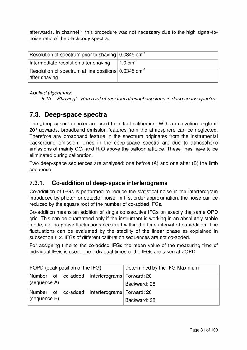
Resolution of spectrum prior to shaving 0.0345 cm-1
Intermediate resolution after shaving 1.0 cm-1
Resolution of spectrum at line positions
after shaving
0.0345 cm-1
Applied algorithms: 8.13 ‘Shaving’ - Removal of residual atmospheric lines in deep space spectra
7.3. Deep-space spectra
The „deep-space“ spectra are used for offset calibration. With an elevation angle of
20° upwards, broadband emission features from the atmosphere can be neglected.
Therefore any broadband feature in the spectrum originates from the instrumental
background emission. Lines in the deep-space spectra are due to atmospheric
emissions of mainly CO2 and H2O above the balloon altitude. These lines have to be
eliminated during calibration.
Two deep-space sequences are analysed: one before (A) and one after (B) the limb
sequence.
7.3.1. Co-addition of deep-space interferograms
Co-addition of IFGs is performed to reduce the statistical noise in the interferogram
introduced by photon or detector noise. In first order approximation, the noise can be
reduced by the square root of the number of co-added IFGs.
Co-addition means an addition of single consecutive IFGs on exactly the same OPD
grid. This can be guaranteed only if the instrument is working in an absolutely stable
mode, i.e. no phase fluctuations occurred within the time-interval of co-addition. The
fluctuations can be evaluated by the stability of the linear phase as explained in
subsection 8.2. IFGs of different calibration sequences are not co-added.
For assigning time to the co-added IFGs the mean value of the measuring time of
individual IFGs is used. The individual times of the IFGs are taken at ZOPD.
POPD (peak position of the IFG) Determined by the IFG-Maximum
Number of co-added interferograms
(sequence A)
Forward: 28
Backward: 28
Number of co-added interferograms
(sequence B)
Forward: 28
Backward: 28

Page 32 of 100
The preceding steps are performed separately for the interferograms taken at
forward and backward movement of the interferometer, respectively.
Applied algorithms:
8.2 Co-addition of interferograms
7.3.2. Phase determination of deep-space spectra
The quality of the phase determination is enhanced by applying the statistical phase
determination approach described in detail in chapter 6.2.
The complex spectrum used in all steps of this phase determination method is
derived by a classical real FFT from the interferogram I(x) which is degraded by the
apodisation function A(x).
( ) ( ) ( )S A x IFG xFT+ σ =
A high-pass digital filtering is performed by convolution of the spectrum with a kernel
function describing the filter.
The kernel represents the coefficients of a non-recursive, digital filter for evenly
spaced data points. The kernel coefficients are Kaiser-weighted. The intensity of the
Gibbs phenomenon wiggles are defined in -db; a value of 50 or more should be
appropriate.
order of the kernel 20
reduction of the Gibbs phenomena 50 dB
lower frequency of the filter in
fractions of the Nyquist frequency
0.4
low wavenumber of bandwidth
interval
660 cm-1 1000 cm-1 1540 cm-1 1720 cm-1
high wavenumber of bandwidth
interval
980 cm-1 1600 cm-1 1800 cm-1 2500 cm-1
instrumental phase function As defined in subsection 7.2.1
max. residual uncertainty of the
phase for iteration stop
20mrad
Maximum number of iterations 25
Applied algorithms:
8.11.3 Statistical phase determination
7.3.3. Phase correction of deep-space interferograms
� See subsection 7.2.2, but the phase information is taken from the process
described in the preceding section 7.3.2

Page 33 of 100
7.3.4. Generation of deep-space spectra
The same processes are used as described in the section about blackbody spectra,
(see subsection 7.2.3). The parameterisation is listed below:
Resolution of deep space spectra 0.0345 cm-1
Length of interferogram (OPD) used +/- 14.5 cm
Apodisation Norton-strong (Contract 11717_95_NL_CN)
Rectangle (Contract 12078_96_NL_GS)
Applied algorithms:
8.7 Generation of spectra
7.3.5. Shaving of deep-space spectra
The "shaving" of spectra is necessary to remove any sharp spectral lines from the
deep space spectra that are formed in the atmosphere above the balloon. The
"shaving" is performed in the same manner as the "shaving" of blackbody spectra
described in subsection 7.2.5, but in case of deep space spectra the lines are not
reinserted afterwards.
The instrumental contribution to lines in the deep-space spectra can be neglected
since their influence in the calibration procedure is of second order.
Resolution of spectrum prior to shaving 0.0345 cm-1
Resolution of spectrum after shaving 1.0 cm-1
Applied algorithms:
8.13 ‘Shaving’ - Removal of residual atmospheric lines in deep space
spectra
7.4. Limb sequence spectra
For the processing of the limb spectra, the first three steps are identical to the
processing of deep space spectra, so for
7.4.1. Phase determination of limb sequence spectra
� See subsection 7.3.2
7.4.2. Phase correction of limb sequence interferograms
� See subsection 7.2.2

Page 34 of 100
7.4.3. Generation of limb sequence spectra
� See subsection 7.3.3
7.5. Calibration
7.5.1. Radiometric calibration of limb spectra
The radiometric calibration allows to convert the uncalibrated values into physical
units of spectral radiance as described in Subsection 6.3. A two point calibration is
performed. One calibration point is the offset spectrum Sinstr. which is determined from
‘shaved’ deep-space spectra. The other calibration 'point' is a spectrum of the
relatively ‘hot’ blackbody (SBB, ~210K). Offset and blackbody spectra are interpolated
to the time of the atmospheric measurement. Since all spectra are already phase
corrected the individual phase relation of the interferograms has no significance.
The emissivity of the blackbody is characterized by 0.9986±0.0006. This leads
together with an uncertainty of the temperature measurement to an uncertainty of
gain calibration of maximal 0,23%±0,43% [Trie2000 (The temperature gradient along
the blackbody cylinder is negligible].
At spectral positions of line features in the blackbody spectra the error budget is
significantly higher. Therefore these spectral positions should be omitted for the
retrieval of p, T an trace gases. A list of these spectral positions is given in Appendix
10.1
Applied algorithms:
8.12 Radiometric calibration of the spectra
Page 35 of 100
Channel 1 Channel 2 Channel 3 Channel 4
Radiance of the blackbody
LBB(T=220K) 4,5*10
-6 -
1,9*10-6
1,7*10-6
-
3,0*10-7
1,5*10-7
-
6,8*10-8
5,6*10-8
-
1,9*10-8 1 2
W
cm sr cm−
Absolute noise of the baseline
Error due to
noise in the
blackbody
spectra in the
limb
spectra
ATM NESRL ,∆
7*10-9 2*10-9 3*10-9
2*10-9
1 2
W
cm sr cm−
∆ϕtot,ATM =
0,002 (710cm-1
)
.. 0,023 (1000cm-1
)
∆ϕtot,ATM =
0,0008 (1040cm-1
)
.. 0,012 (1600cm-1
)
∆ϕtot,ATM =
0,0095 (1641cm-1
)
.. 0,037 (1800cm-1
)
rad
Error due to
phase
inaccuracies
in the limb
spectra.
ATMATML ,ϕ∆
7,4*10-10
..
1,4*10-8
3,7*10-11
..
5,0*10-10
3,1*10-11
..
7,7*10-11 3,7*10
-10 1 2
W
cm sr cm−
∆ϕtot,DS =
0,003 (696cm-1
)
.. 0,050 (1000cm-1
)
∆ϕtot,DS =
0,003 (1037cm-1
)
.. 0,059 (1600cm-1
)
∆ϕtot,DS =
0,027 (1600cm-1
)
.. 0,086 (1800cm-1
)
rad
Error due to
phase
inaccuracies
in the deep-
space
spectra.
DSATML ,ϕ∆
8,7*10-10
-
border of spectral
range:
3,0*10-8
3,3*10-11
-
border of spectral
range:
1,7*10-9
7,6*10-11
-
1,4*10-10
3,7*10
-10
1 2
W
cm sr cm−
Geometric
sum
7,9*10-9
-
3,3*10-8
2,0*10-9
-
2,7*10-9
3,0*10-9
-
3,0*10-9 2,1*10
-9 1 2
W
cm sr cm−
Rel. error of the baseline
S/NBB = 1240 S/NBB = 1730 S/NBB = 235 S/NBB = 63 BBATM
ATM
L
L
,ϕ∆
6,9*10-3
1,5*10-3
8,3*10-3
0,047 %
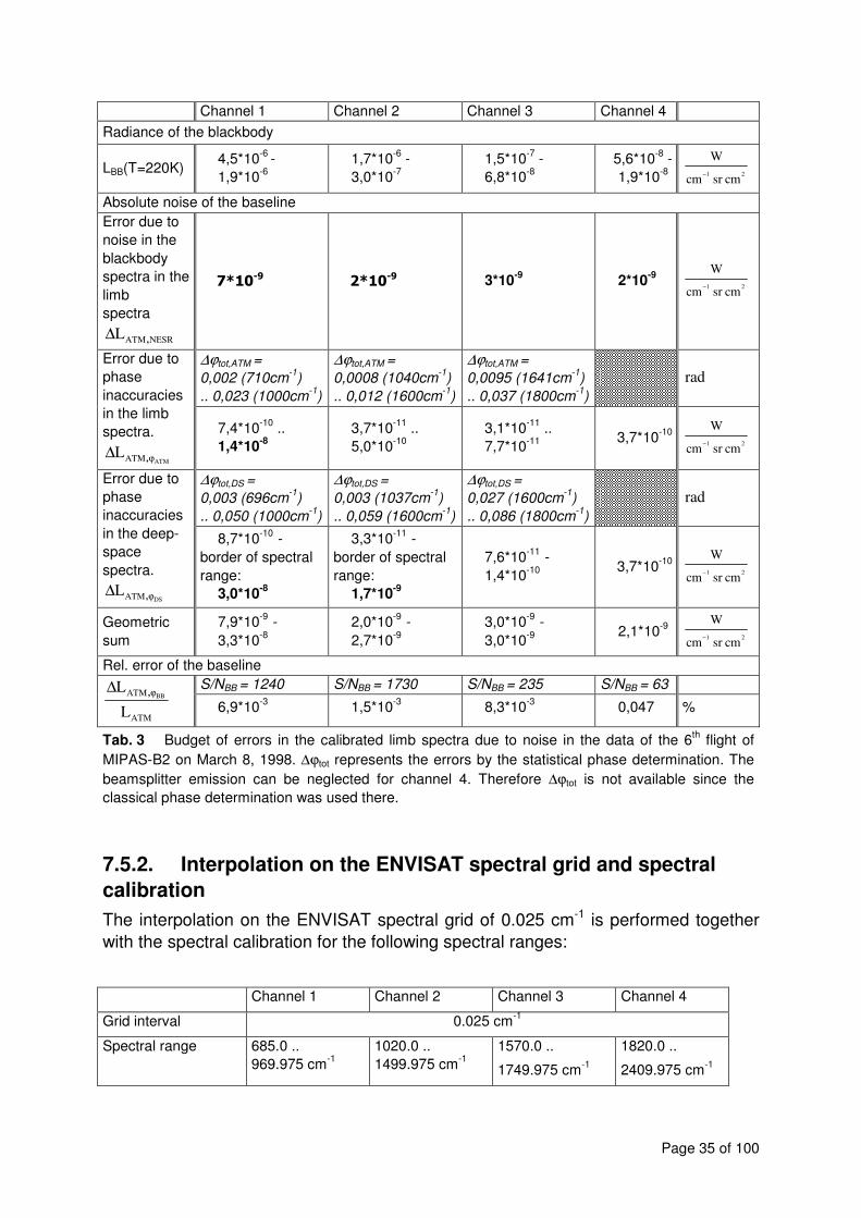
Tab. 3 Budget of errors in the calibrated limb spectra due to noise in the data of the 6th flight of
MIPAS-B2 on March 8, 1998. ∆ϕtot represents the errors by the statistical phase determination. The
beamsplitter emission can be neglected for channel 4. Therefore ∆ϕtot is not available since the
classical phase determination was used there.
7.5.2. Interpolation on the ENVISAT spectral grid and spectral
calibration
The interpolation on the ENVISAT spectral grid of 0.025 cm-1 is performed together
with the spectral calibration for the following spectral ranges:
Channel 1 Channel 2 Channel 3 Channel 4
Grid interval 0.025 cm-1
Spectral range 685.0 ..
969.975 cm-1
1020.0 ..
1499.975 cm-1
1570.0 ..
1749.975 cm-1
1820.0 ..
2409.975 cm-1

Page 36 of 100
Spectral calibration has been obtained by retrievals in a set of spectral intervals
distributed over the whole spectral range using the HITRAN database. From these
retrievals the linear correction functions corr. 0 1 meas.c cσ = + σ have been determined. The
coefficients of which and the standard deviation of the spectral shift values from the
linear function are:
Channel 1 Channel 2 Channel 3 Channel 4
C0 [cm-1
] -0.05112 -0.0496435 -0.1318345 -0.05672
C1 3.95771e-5 1.85948e-5 6.190211E-05 1.29845E-05
uncertainty of spectral
calibration [cm-1
]
5.3e-4 6.3e-4 2.6e-3 1.1e-3
7.5.3. Calculation of variance of single consecutive spectra
The standard deviation is calculated from consecutive calibrated spectra (subsection
7.5.2) of a certain elevation angle. The standard deviation corresponds to the overall
instrument NESR which is photon noise limited. The variance, the diagonal elements
of the variance/covariance matrix, is obtained by the square of the standard deviation
values.
The off-diagonal elements of the covariance matrix are defined by the numerical
apodisation function [Carlotti 1998] since the dominating noise in the interferogram is
not affected by the self-apodisation. The total noise is dominated by the photon noise
of the d.c. level which is of much larger intensity than the modulated part of the
interferogram. Therefore the total noise does not correlate with the modulated part of
the interferogram. This also means, that the magnitude of noise in the interferogram
is constant over the whole optical path. Since this dominating noise in the
interferogram is not affected by the self-apodisation, it is only modulated by the
numerical apodisation function in the interferogram domain.
Applied algorithms:
8.8 Generation of the variance of single consecutive spectra

Page 37 of 100
8. Algorithms - Reference This chapter references the algorithms used for level 1b data processing for MIPAS-
B2. The algorithms are listed in alphabetical order.
The following notation is used within the flowcharts:
In the tables for the definition of variables, the “I/O“ (Input/Output) indication refers to
the following notation:
Notation Description
I input of the process
loop loop or index variable
t temporary or intermediate variable
O output of the process
In the same tables, the “Type“ indication refers to the following notation:
Notation Description
r real number
d date and time
c complex number
i integer number
o ordinal number
t text
Data
Subroutine
path
optional path
loop
Process

Page 38 of 100
8.1. Apodisation functions
Objective
The interferograms may be multiplied with apodisation functions generated within this
subroutine to reduce the ripples of the SINC-function in the spectra originating from
truncated IFG’s.
Eight different apodisation functions are provided:
i24 4
i
i 0 i 0
4
0 045335 0 152442 0 384093x1 0
0 0 136176 0 087577OPD
0 554883 0 983734 0 703484
0 0 0
0 399782 0 0
x 3 x
2OPD 2OPD
A x
0
1
2
3
Norton Beer
Strong Medim Weak
(NS) (NM) (NW)
. . .
. .
. . .
.
cos cos
( )
= =
−
α α − α = α − −
α
α
α
π π + α
=
∑ ∑
( )
22
x 2 x1 1
OPD OPD
xRECT
2OPD
x1
OPD
x1
OPD
for OPD x OPD
0 else
FillerD
=0.18
FillerE
=0.18
Rectangle(RE)
Tapering(TA)
Triangular(TR)
cos cos
α π π
+ + α + α α
−
−
− ≤ ≤

Page 39 of 100
Process flowchart
sizefunction-
name
apodisation
function
output data
Definitions of variables
Variable Description I/O Type Remarks
apod apodisation function type I o possible values:
[NS, NM, NW, FD, FE,
RE, TA, TR]
default value := NS
i,z t i
n number of points of the
interferogram to be apodised
I i n must be odd
A apodisation function O r
c apodisation coefficients t r array of 5 elements

Page 40 of 100
Algorithm
( )
z i
z i
0
z i
0
z i
z i
z n 1 2
i 0 z 1
A
A i z
c 0 18
i 3 iA c
2z 2z
c 0 18
i 2 iA c c
z z
A i z
c 0 384093 0
+
+
+
+
+
= +
∈ −
=
π π
=
π π
/
[ , ]
.
.
. , -
0
0 0
22
with
RE: = 1
TR : = 1- /
FD:
= cos + cos
FE:
= 1+(1+ )cos + cos
TP : = 1-( / )
NW: = [ ]
[ ]
[ ]
j
z i 0 j
j
z i 0 j
z i 0 j
087577 0 703484 0 0 0 0
A c c i z
c 0 152442 0 136176 0 983734 0 0 0 0
A c c i z
c 0 045335 0 0 0 554883 0 0 0 399782
A c c i z
+
+
+
=
=
∑
∑
∑
. , . , . , .
= /
. , - . , . , . , .
= /
. , . , . , . , .
= /
42
j=1
42
j=1
42
j=1
+ 1-( )
NM:
+ 1-( )
NS:
+ 1-( )j
and symmetrising:
A A
A
z i z i− +=
=0 0

Page 41 of 100
8.2. Co-addition of interferograms
Objective
Co-addition of IFGs is performed to reduce the statistical noise in the interferogram
introduced by photon or detector noise. The noise is reduced by the square root of
the number of co-added IFGs.
Co-addition means an addition of single undersampled IFGs in that way, that each
point, which is added refers to exactly the same optical path difference. The IFGs are
aligned to the point of zero optical path difference (ZOPD). This is realized by
assigning the peak position (POPD) of each IFG to the same optical path difference
(OPD). This can be guaranteed only if the instrument is working in an absolutely
stable mode, i.e. that no phase fluctuations occur, no misalignment, no effects of
noise regarding the POPD (see figures in Subsection 6). To check for instrumental
stability, the linear phase of each interferogram is calculated and compared. If the
phase is not equal within a limited range, then the interferogram is discarded from co-
adding.
For assigning time to the co-added IFGs the mean of the measuring times is used.
The individual times of the IFGs are taken close to ZOPD. The same approach is
taken for the localization, the line of sight (LOS) information and the blackbody
temperature.

Page 42 of 100
Process flowchart
Coaddition
ZOPD-
typesingle
IFG
selection
of IFG
IFG coaddition
coadd.
IFG's
calc.meanTime
calc.meanTemp
visualisation
determine
ZOPD Position
check for correct
POPD position
'classical'
phase determination
Definitions of variables
Variable Description I/O Type Remarks
a Number of interferograms to
be co-added
I i default value := 1
maφ offset of the linear phase of
interferogram m
t r
mbφ slope of the linear phase of
interferogram m
t r
A number of co-added IFG’s O i initial value := 0
bm BB-temperature of single ifgm I r
B mean BB-temperature of co-
added IFG
O r initial value := 0
c type of derivation of the I o possible values:

Page 43 of 100
POPD [maxpeak, nompeak,
user defined]
default val. := maxpeak
dxm sampling interval of ifgm I r
ifgmi point i within ifgm I r
IFGi point i within the co-added
IFG
O r initial value :=0
m index of the single
Interferogram
t i range:
[0..a-1]
nm number of points of ifgm I i
N number of points of the co-
added IFG
O i
tm time at ZOPD of single
interferogram
I d
T mean time at ZOPD of co-
added IFG
O d initial value:
greg2julian(T) := 0
zm point of POPD in ifgm t i range:
[0..nm-1]
Z position of the POPD of the
co-added IFG
O i
i index variables t i
j number of points of the left
side of the IFG
t i
k number of points of the right
side of the IFG
t i
pm nominal peak position of ifgm I i range [0..nm-1]
qm user defined peak position of
ifgm
I i range [0..nm-1]
ε a range in which the phase
offset may vary
I r default value := π/4
ε b range in which the phase
slope may vary
t r default value :=
m
1
4 2dx
π
Algorithm
Selection of IFG’s
A selection of the IFGs to be co-added is done according to dxm. Any ifgm with dxm
not equal dx1 is discarded from co-adding.

Page 44 of 100
Determine POPD position
Depending of the value of c, the POPD position is identified as the position of the
maximum positive value within the IFG or as the nominal peak position as defined by
the optical setup and the hardware.
m
i
m m
m
index_of(max(ifg )) if c maxpeak
z p if c nompeak
q if c user defined
=
= = =
Check for instrumental stability
To check for instrumental stability, the linear phase of each interferogram (index m) is
calculated with the 'classical' phase determination and is compared to the phase of
the first interferogram (index 0). If the difference of the offset a or slope b of the linear
phase is larger than εa respectively εb, then the interferogram is discarded from co-
adding. With the factor of m
11
2dx the criterion εb for the slope the limitation is
automatically aligned to the sampling distance. In the case that the true maximum is
located in the middle between two sampling points, then the slope of the phase may
switch between dx±π . To avoid this a default limit of the slope variation of dx2
π was
chosen.
0 m 0 m
a bco-addition, if a a b b− < ε ∧ − < ε
Co-addition
Performs the co-addition of the IFGs, shifted that way, that all POPD points will be on
top of the other. This could lead to points at the far ends of the IFG to be co-added,
for which no corresponding data point exist in the already co-added IFG. Therefore,
the overall co-added IFG is limited to the largest common set of data points of all
individual IFGs.
The normalisation of the co-added IFG is done during every co-addition step to allow
a continuous visualisation of the co-addition process.
During every iteration of the co-addition process the mean temperature B of the
blackbody and the mean measuring time T is calculated.

Page 45 of 100
1AA
1kjN
jZ
1A
bBAB
1A
tTAT
kjifor1A
ifgIFGAIFG
0Aif
0Aif
1zn1ZN
1znk
0Aif
0Aif
zZ
zj
m
m
izm
iZij
mm
mm
m
m
m
+=
++=
=
+
+×=
+
+×=
−=+
+×=
>
=
−−−−
−−=
>
=
=
+++
)julian(2greg)julian(2greggreg2julian
],[
],min[
],min[
Loop
A loop over all interferograms to be co-added is performed.
From m=0 to a-1 do begin
Selection of interferograms from the database
Determination of POPD position
Co-addition
end

Page 46 of 100
8.3. Co-addition of spectra
Objective
Co-addition in the spectral domain is performed to reduce the noise in the spectra. It
has the same functionality as the co-addition of the Interferograms, but usually the
spectra are already based on phase corrected IFG’s. Therefore the problem of phase
instabilities doesn’t have to be taken into account. The noise is reduced by a factor of
A1/2 (A: number of co-added spectra). For co-addition in the spectral domain all
spectra have to be on the same spectral grid, means that each point, which is added
refers to an identical wavenumber.
Process flowchart
Coaddition
spectral
rangespectra
selection
of Spectra
spectra
coadding
outputdata
calc.
meanTime
calc.
meanTemp
visualisation
determine the
wavenumber abscissa
calc. sums
for variance

Page 47 of 100
Definitions of variables
Variable Description I/O Type Remarks
a number of spectra to be co-
added
I i defined by the number
of selected spectra
A number of co-added spectra O i
dσm wavenumber interval
(spectral spacing) within sm
I r defined by the first
spectrum of the set of
spectra to be co-added
smi point i within sm I r
Si point i within the co-added
spectrum S
O r
m index of s t i
N number of points of the co-
added spectrum S
O i
σmL lowest wavenumber in sm t r
σmH highest wavenumber in sm t r
σL lowest wavenumber in the co-
added spectrum
t r
σH highest wavenumber in the
co-added spectrum
t r
i,j,k index variables t i
loop loop variable t is true if spectra for co-
adding are available
Algorithm
Selection of spectra
The spectra to be co-added need to have exactly the same spacing of the spectral
points. A selection of the spectra to be co-added is done according to dσm. Any Sm
with dσm not equal to dσ1 is discarded from co-adding.
Determination of wavenumber abscissa
It is not absolutely necessary to have the same lower and higher bandwidth edges.
Only common spectral points of the single spectra will be used for co-adding.
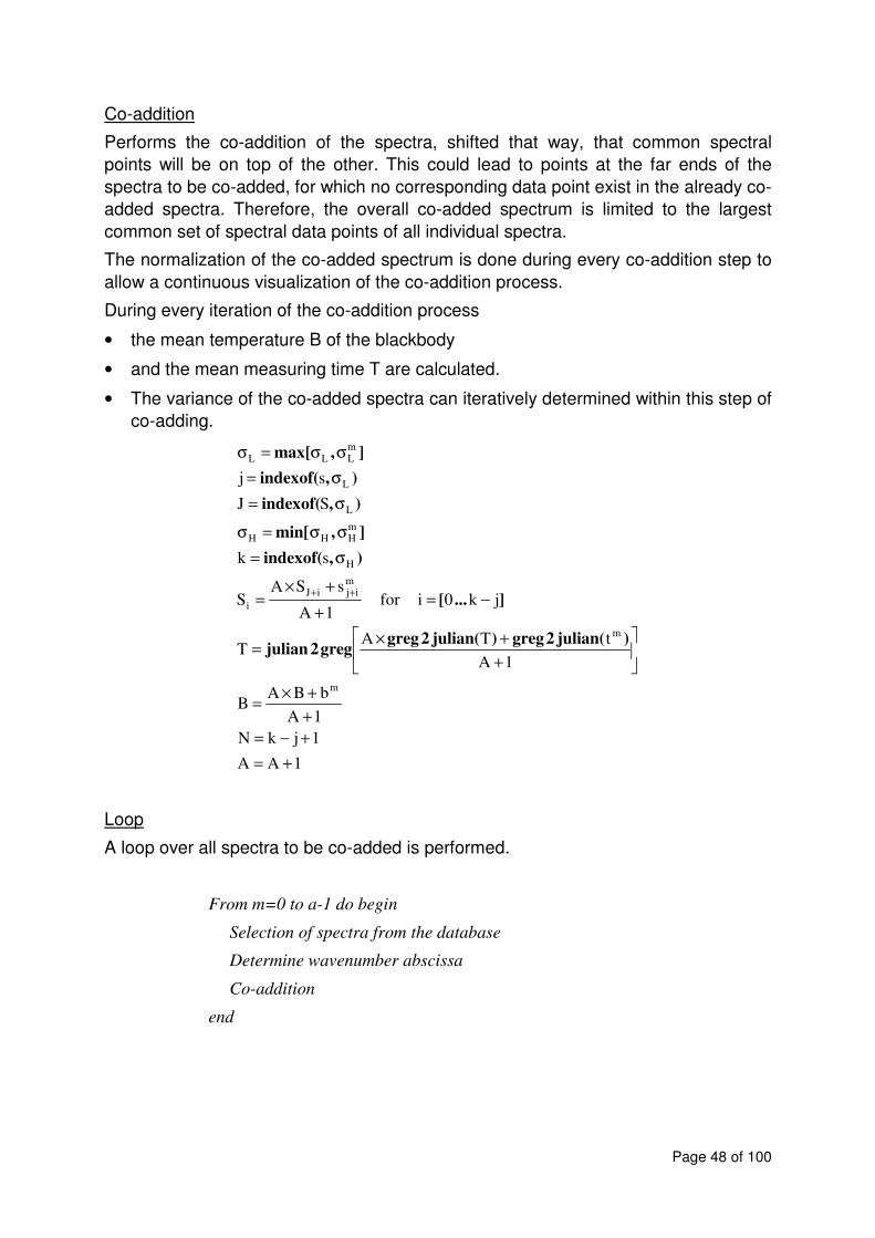
Page 48 of 100
Co-addition
Performs the co-addition of the spectra, shifted that way, that common spectral
points will be on top of the other. This could lead to points at the far ends of the
spectra to be co-added, for which no corresponding data point exist in the already co-
added spectra. Therefore, the overall co-added spectrum is limited to the largest
common set of spectral data points of all individual spectra.
The normalization of the co-added spectrum is done during every co-addition step to
allow a continuous visualization of the co-addition process.
During every iteration of the co-addition process
• the mean temperature B of the blackbody
• and the mean measuring time T are calculated.
• The variance of the co-added spectra can iteratively determined within this step of
co-adding.
Loop
A loop over all spectra to be co-added is performed.
From m=0 to a-1 do begin
Selection of spectra from the database
Determine wavenumber abscissa
Co-addition
end
1AA
1jkN
1A
bBAB
1A
tTAT
jk0ifor1A
sSAS
sk
SJ
sj
m
m
mijiJ
i
H
mHHH
L
L
mLLL
+=
+−=
+
+×=
+
+×=
−=+
+×=
σ=
σσ=σ
σ=
σ=
σσ=σ
++
)julian(2greg)julian(2greggreg2julian
]...[
),indexof(
],min[
),indexof(
),indexof(
],max[
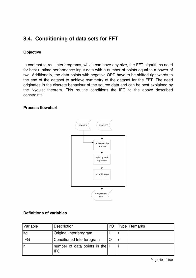
Page 49 of 100
8.4. Conditioning of data sets for FFT
Objective
In contrast to real interferograms, which can have any size, the FFT algorithms need
for best runtime performance input data with a number of points equal to a power of
two. Additionally, the data points with negative OPD have to be shifted rightwards to
the end of the dataset to achieve symmetry of the dataset for the FFT. The need
originates in the discrete behaviour of the source data and can be best explained by
the Nyquist theorem. This routine conditions the IFG to the above described
constraints.
Process flowchart
Definitions of variables
Variable Description I/O Type Remarks
ifg Original Interferogram I r
IFG Conditioned Interferogram O r
n number of data points in the
IFG
I i
new size input-IFG
defining of the
new size
conditioned
IFG
recombination
splitting and
expansion

Page 50 of 100
m log2 of the size/2 of the output
data
t i
s max. output length of the
conditioned IFG
I/O i default input value : s is
not limited
t1 right part of the IFG (x>0) t r
t2 left part of the IFG (x<0) t r
z point of POPD I i
Algorithm
Definition of the new size
( ) ( )2m log max[z, n z , s / 2 ]= −
Splitting and extension
0t
ifgt
0t
ifgt
1z202
1z012z22
12zn1
1nz1zn01
m
mm
m
=
=
=
=
−−
−−−
−−
−−−
..
....
..
....
Recombination
1202
122
1201
120
m1mm
mm
tIFG
tIFG
−−
−−
=
=
+ ....
....

Page 51 of 100
8.5. Convolution of data sets using FFT
Objective
The mathematical convolution of two functions can be performed by using the
‘convolution theorem’.
[ ] [ ]g f k f kFFT FFT FFT− + + = ⊗ =
If the number of points of the convolution kernel is larger than
( )2log N , N : number of points of the function f
a convolution by using FFT is appropriate to save computation time.
Process flowchart
<none>
Definitions of variables
Variable Description I/O Type Remarks
f source function I r
k convolution kernel I r
g result O r
Algorithm
<library routine>

Page 52 of 100
8.6. Fitting procedure with weighting coefficients
Objective
This function performs a weighted least-squares polynomial fit by using matrix
inversion. It is used to fit a polynomial to a one-dimensional vector by assigning the
individual points of the vector with different weights.
This routine is a classical library function.
Process flowchart
<none>
Definitions of variables
Variable Description I/O Type Remarks
data Input/output-data I/O r
w weighting parameter I r w=0: no weighting
w≠0: the power with
which the weighting
function is to be raised.
r wavenumber range in which
the fit has to be applied
I r default value is the
overall spectral range of
the input spectrum
o the order of the polynom to
be fitted
I i default value := 1 (linear
function)
f weighting function I r Must have the same
abscissa as the input -
data
Algorithm
<library routine>
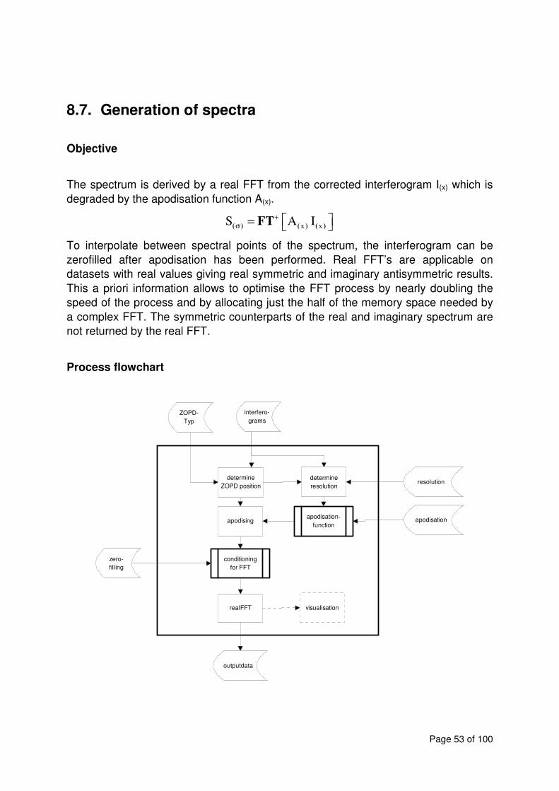
Page 53 of 100
8.7. Generation of spectra
Objective
The spectrum is derived by a real FFT from the corrected interferogram I(x) which is
degraded by the apodisation function A(x).
x xS A I( ) ( ) ( )FT+σ
=
To interpolate between spectral points of the spectrum, the interferogram can be
zerofilled after apodisation has been performed. Real FFT’s are applicable on
datasets with real values giving real symmetric and imaginary antisymmetric results.
This a priori information allows to optimise the FFT process by nearly doubling the
speed of the process and by allocating just the half of the memory space needed by
a complex FFT. The symmetric counterparts of the real and imaginary spectrum are
not returned by the real FFT.
Process flowchart
realFFT
ZOPD-
Typ
interfero-
grams
determine
ZOPD position
outputdata
visualisation
conditioning
for FFT
apodisation-
function
resolution
apodising
determine
resolution
zero-
filling
apodisation

Page 54 of 100
Definitions of variables
Variable Description I/O Type Remarks
apod apodisation function I r
c type of derivation the POPD I o Values:
[maxpeak, nompeak,
user defined]
default val. := maxpeak
dx sampling interval within ifg I r
Ifgi point i within ifg I r
IFG apodised and conditioned
IFG for FFT
O r
k number of points of a single
side of the IFG according to
the selected resolution
t i
n number of points of IFGm I i
N number of complex points in
the spectrum
O i
p nominal peak position of ifgm t i range [0..n-1]
q user defined peak position of
ifgm
I i range [0..n-1]
γ resolution I r in cm-1
Γ nominal resolution O r in cm-1
z point of selected POPD in
IFG
t i Range: [0..n-1]
S spectrum O c
i,j,k index variables t i
Algorithm
Determine POPD position
Depending of the value of c the POPD position is identified as the position of the
maximum positive value within the IFG or as the nominal peak position as defined by
the optical setup and the hardware.
iindex_of(max(ifg )) if c maxpeak
z p if c nompeak
q if c user defined
=
= = =

Page 55 of 100
Determine resolution
The highest possible resolution is chosen, considering the constraints of the desired
input value for the resolution and the length of the interferogram before and after the
POPD.
( )1 1
2cdx 2 n c 1 dx
1k
2 dx
max , ,
Γ = γ − −
=Γ
Apodising
Performs the multiplication of the IFG with the apodisation function, shifted that way,
that the symmetry point of the apodisation function will be shifted to the POPD of the
IFG.
[ ]i i z k iIFG A ifg for i 0 2k 1,− += = −
Real-FFT:
As FFT a so called ‘real FFT’ is used, which has as input only a real input array. The
result is a complex function with the real part transformed from the even part of the
IFG and the imaginary part transformed from the odd part of the IFG.
The implementation is described in [Pres1986].
)realfft(IFGS =

Page 56 of 100
8.8. Generation of the variance of single consecutive
spectra
Objective
The variance is used to determine the impact of statistical noise onto the co-added
spectrum.
( )N 2
i n i
n 1i
S S
N 1
,
=
−
ν =−
∑
For memory reasons it is advantageous to obtain the variance iteratively with each
step of co-addition of the calibrated spectra.
The equation to determine the variance can be rewritten with
2N N
2
i n i n
n 1 n 1
i
S S N
N 1
, ,
= =
− ν =
−
∑ ∑ .
The two sums and in the equation above can be added separately at each iteration
step.
N
i n
n 1
N2
i n
n 1
D0 S
D1 S
,
,
=
=
=
=
∑
∑
The variance is then calculated at the end of the iteration by
2
i
D1 D0 N
N 1
−ν =
−

Page 57 of 100
Process flowchart
calibrated
spectra
calc. of the
sums D1 and
D2
number
of spectra
number
of
spectra
D0, D1
calc. of
variance
output data
D0, D1

Page 58 of 100
Definitions of variables
Variable Description I/O Type Remarks
S Individual spectrum of the co-
added spectrum
I r
i point within single spectrum,
element of the matrix
t i
n indices of the spectrum t i Range: 1..N
ν covariance matrix O r
D0 sum t/I r
D1 sum of squares t/I r
N number of spectra I i defined by the number
of selected spectra
Algorithm
Calculation of the sums D0 and D1
This process can be started on each calibration process. It has to be validated that all
calibrated spectra have the same wavenumber axis. The calculation of the sums is
normally performed during co-addition of the calibrated spectra (Subsection 8.3), but
can also be performed separately.
N
i n
n 1
N2
i n
n 1
D0 S
D1 S
,
,
=
=
=
=
∑
∑
Calculation of the variance
The variance is then calculated at the end of the iteration over all calibrated spectra
by
2
i
D1 D0 N
N 1
−ν =
−

Page 59 of 100
8.9. Interferogram correction and mathematical filtering
Objective
The phase disturbed IFG is corrected such that the desired spectrum is purely real
and any beamsplitter contributions are purely imaginary. Within this process the
bandwidth of the spectrum can be limited by a mathematical band-pass filter b(σ).
x
i
corr
i
corr x x
i
x
i
corr x x
k
S S e b
IFG ifg e b
ifg e b
IFG ifg e b
( )
( )
( )
( )
*( )
( ) ( ) ( )
( ) ( ) ( )
( ) ( )
( ) ( ) ( )
FT FT
FT FT
FT
σ
σ
σ
σ
Φ
σ σ σ
Φ
σ
Φ
σ
Φ
σ
=
=
= ⊗
⇒
= ⊗ 1442443
The resulting kernel l(x) is optimised by the tapering function A(x) to reduce the
wiggles of the Gibb’s phenomena. The tapering function can be any apodisation
function.
xx xk k A*( )( ) ( )=
The corrected IFG is performed by a convolution of the disturbed IFG with the kernel
k(x).
corr x x xIFG ifg k( ) ( ) ( )= ⊗

Page 60 of 100
Process flowchart
Definitions of variables
Variable Description I/O Type Remarks
m index t i
b Mathematical band-pass-filter I r default is no bandpass
limitation
Φ phase function I r
ifg Input interferogram I r
apod Tapering-function I possible values:
[NS, NM, NW, FD, FE,
RE, TA, TR]
default value := NS
IFG Corrected Interferogram O r
k kernel function t r
Algorithm
The routine uses no specific algorithm. See Subsection 8.10 and 8.5 for kernel
generation and convolution
Outputdata
interfero-
gram
phase-
function
kernel
generation
mathematical
filter
visualisation
convolution
apodisation
function

Page 61 of 100
8.10. Kernel generation
Objective
For phase correction of interferograms a convolution kernel is needed:
The phase disturbed IFG is corrected by a given phase Φ(σ). During this process the
spectrum can be limited by a mathematical band-pass filter b(σ). Both parameters
are given in the spectral domain which are to be transformed into the space domain.
( )i*
(x) ( )k FT[e b ]σΦ
σ=
The resulting kernel l(x) is optimized by the tapering function A(x) to reduce the
wiggles of the Gibb’s phenomena. The tapering function can be any apodisation
function.
(x ) (x) (x)k k * A=
Process flowchart
Outputdata
phase-
function
generate kernel
mathematical
filter
apodisation
function
apodisation
symmetrising

Page 62 of 100
Definitions of variables
Variable Description I/O Type Remarks
m index t i
b bandpassfilter I default is no bandpass
limitation
Φ phase function I
t temporary vector t
k* non-apodised kernel t
N number of points of the phase
function
I
k kernel function O
Algorithm
Generating the kernel
The bandwidth filtering vector b is adjusted to have the same abscissa as the phase
function Φ, which again must have the same abscissa as the Fourier transformed of
interferogram which is to be phase-corrected.
mi
m mt e b
t FFT(t)
Φ=
=
Symmetrising
The correction function has to be symmetrised around the center point at N/2 of the
vector t:
1N2N12N0
12N01N2N
tk
tk
−−
−−
=
=
.../*
/...
/...*
.../
The final kernel function k is apodised to reduce the wriggles in the spectrum due to
the band-pass filter.

Page 63 of 100
8.11. Phase determination
Objective
<as described in chapter 6.2>
Process flowchart
'classical' phase
determination
predefined
instrumental phase interferogramm
'statistical' phase
determination
'differential' phase
determination
Phase
final result
parameters
for the
'statistical'
phase
fit-parameters
phase 2. level
phase for initialisation
phase
1. level
vert. boundary
fit-parameters
1. level
2. level
3. level

Page 64 of 100
8.11.1. ‘Classical’ phase determination
Objective
The phase is obtained by the angle between the real and imaginary part of the
complex spectrum S(σ) (classical approach by [Form1966]). The spectrum is derived
by a FFT from the interferogram I(x) which is degraded by the apodisation function
A(x).
( ) ( )
( )
( )
( ) x x
x
c( )
x
S FT A I
Im Sarctan
Re S
+σ
σ
=
φ =
The noise in the spectrum is propagated to the phase function which should be a
smooth and noiseless function. Therefore the phase function is fitted with a well
defined instrumental phase, derived from a black-body measurement. Only linear
phase shifts could be reasonably determined, so that a first order linear square fit is
performed. At spectral points where the interferometer ports are well balanced, the
phase is ill defined. This appears mostly at low spectral radiances of the scene.
Therefore, to reduce these effects, the phase points to be fitted are weighted by the
square of the absolute spectral intensity.

Page 65 of 100
Process flowchart
output data
fit range
weighting-
para-
metrisation
ZOPD-
type
input
data
spectrum
generation
resolution,
apodisation
'classical'
phase
weighting of
phase points
and
fitting
fit para-
metrisation
visualisation
instrumental
phase
function
zerofilling
= 1
subtraction
addition
Definitions of variables
Variable Description I/O Type Remarks
apod apodisation function type I r Values:
[NS, NM, NW, FD, FE,
RE, TA, TR]
default value := NS
c type of derivation of the
POPD
I o possible values:
[maxpeak, nompeak,
user defined]
default val. := maxpeak
dx sampling interval within ifg I r
i index variables t i range: [0..m-1]

Page 66 of 100
ifgi point i within ifg I r
m number of complex points in
spectrum S
t i
n number of points of IFGm I i
o the order of the polynom to
be fitted
I i range: [0..5]
default: Linear function
r wavenumber range in which
the fit has to be applied
I r see subsection 7
Si point i of complex spectrum S t c
w weighting parameter I r default value := 2
Z zerofilling t i Z=1, means no
zerofilling is used
Φi point i within the phase
function Φ
O,t r
γ resolution I r default is the max.
resolution defined by the
length of the IFG
Algorithm
Classical phase
The arc-tangent function returns the phase angle of the complex spectrum,
expressed in radians. The range of the phase is between -π and π.
( ) ( ) [ ]
[ ]i i i iarctan Re S , Im S ,
i 0..m 1
withφ = φ ∈ −π π
= −

Page 67 of 100
8.11.2. Differential Phase determination
Objective
The 'differential' phase [Wedd1993] is defined as the angle between the derivatives
of the imaginary and real part of the complex spectrum. The spectrum to be
determined is derived by a complex FFT of the interferogram I(x) which is degraded
by the apodisation function A(x).
( ) (x) (x)
( )
d( )
( )
S FT (A I )
SIm
arctanS
Re
+σ
σ
σσ
=
∂
∂σ Φ = ∂
∂σ
The differential phase is fitted the same way as described in the paragraph of the
‘classical’ phase approach.

Page 68 of 100
Process flowchart
output data
fit range
weighting-
para-
metrisation
ZOPD-
type
input
data
spectrum
generation
resolution,
apodisation
differential
phase
weighting of
phase points
and
fitting
fit para-
metrisation
visualisation
instrumental
phase
function
vertical
limiting
vert. limiting
phase, vert.
boundary
zerofilling
= 1

Page 69 of 100
Definitions of variables
Variable Description I/O Type Remarks
apod apodisation function type I r Values:
[NS, NM, NW, FD, FE,
RE, TA, TR]
default value := NS
c type of derivation of the
POPD
I o Values:
[maxpeak, nompeak,
user defined]
default val. := maxpeak
dx sampling interval within ifg I r
i index variables t i range: [0..m-1]
ifgi point i within ifg I r
m number of complex points in
spectrum S
t i
n number of points of IFGm I i
o the order of the polynom to
be fitted
I i range: [0..5]
default: linear function
r wavenumber range in which
the fit has to be applied
I r see subsection 7
Si point i of complex spectrum S t c
S'i Derivative of S t c
w weighting parameter I r default val. := 2
Z zerofilling t i Z=1, means no
zerofilling is used
Φi* point i within the phase
function Φ* obtained from the
derivative
t r Range: [–π/2 .. π/2]
ΦS,i point i within the initial phase
function ΦS
I,t r
Φi point i within the diiferential
phase function Φ
O,t r
γ resolution I r default is the max.
resolution defined by the
length of the IFG

Page 70 of 100
Algorithm
Differential phase
The arc-tangent function returns the phase angle of the derivated complex spectrum,
expressed in radians. The range of the phase is between –π/2 and π/2.
[ ]
[ ]
i 1 i 1i
i i i
i
S SS
2dx
arctan Im(S ) Re(S )
with
[ 2, 2]
i 1..m 2
+ −
∗
∗
−′ =
′ ′Φ =
Φ ∈ − π π
= −
Vertical limiting
Since the arctan is repetitive with π, therefore the phase may jump about π, when the
real part of the derivative is changing sign. To reduce this effect a vertical boundary
band is introduced which is a defined by the initial phase ±π/2.
i i S,i S,iarctan tan ∗ Φ = Φ − Φ + Φ

Page 71 of 100
8.11.3. Statistical phase determination
Objective
Noise in the differential spectra may deteriorate the accuracy of the differential
phase, especially in case of single non-co-added spectra. This affects the accuracy
of the phase corrected spectrum to an unacceptable level.
The quality of the phase retrieval can be enhanced by applying some a-priori
constraints:
• As already explained, the total phase-function can be separated into a
instrumental part Φ*(σ) and a linear part ∆Φ(σ). The second one can be expressed
as a straight line with the parameters offset a and slope b.
0= a + b( - )*( ) ( ) ( ) ( )σ σ σ σΦ = Φ + ∆Φ Φ + σ σ
• the correlation between the atmospheric and the beamsplitter spectrum has to
vanish:
= ( (S), (S)) 0correl Re Imµ → ±
To avoid the correlation between the imaginary and real part of the spectra with
respect to the spectral response (due to the Planck- and filter-function), each part
is highpass filtered.
• the variance of the beamsplitter spectrum has to be minimised. For better
convergence the elements of the variance are squared:
( )
* *
2 2
4
i ,i ,i
d d variance(Im (S)) = = 0
d( ) d( )
Im(S ) + Re(S )d =
d( )
Φ Φ
ν
∆Φ ∆Φ
∆Φ∑ ∆Φ
A solution is found, if:
( )
( )0
0
2
2
=∂
∂
=∂
∂
b
a
ν
ν
The correlation µ converges rapidly for the phase-offset a. But for the slope b the
positive line correlations of one side of the spectral band may be compensated by
negative line correlations of the other side. On the other hand ν does not converge
rapidly for the offset a but for the slope b. A combination at each iteration step of µ for
the offset and of ν for the slope b results in a good convergence for both parameters.
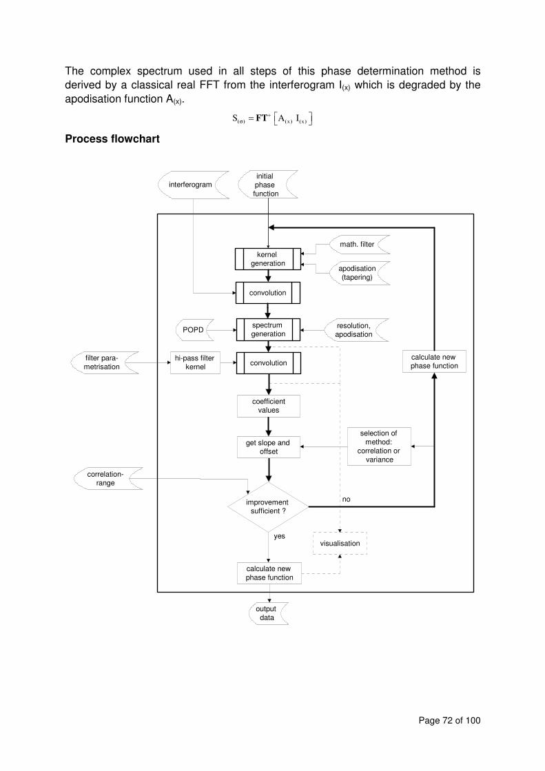
Page 72 of 100
The complex spectrum used in all steps of this phase determination method is
derived by a classical real FFT from the interferogram I(x) which is degraded by the
apodisation function A(x).
x xS A I( ) ( ) ( )FT+
σ =
Process flowchart
output
data
filter para-
metrisation
POPD
interferogram
spectrum
generationresolution,apodisation
coefficientvalues
get slope and offset
visualisation
correlation-range
convolutionhi-pass filter
kernel
initial
phase
function
kernel generation
improvement sufficient ?
no
yes
convolution
math. filter
apodisation
(tapering)
calculate new phase function
selection of
method:
correlation or
variance
calculate new
phase function

Page 73 of 100
Definitions of variables
Variable Description I/O Type Remarks
a offset t r
b slope t r
ci coefficiants for variance and
correlation
t r
fl lower frequency of the filter in
fractions of the Nyquist
frequency
I r default value := 0.4
gibb reduction of the gibb’
phenomena
I r expressed in dB
ki kernel function t r
order order of the kernel I i default value := 100
m index t i
result t b
step iteration t i initial value: step=0
steplimit limit of iteration steps I r default value := 15
zi operator variable t r
α Bessel coefficient t r
εν limit of the variance change
from step to step
I r default value := 2e-4
εµ limit of the correlation change
from step to step
I r default value := 2e-4
εΦ limit of the phase uncertainty I r default value := 20mrad
Φi* instrumental phase function I r
Φi corrected phase function O r
µ correlation coefficient t,O R
ν variance coefficient t,O R
σi wavenumber at point i I r
σL low wavenumber of
bandwidth interval
I r see section 7
σH high wavenumber of
bandwidth interval
I r see section 7
σ0 medium wavenumber of
bandwidth interval
t r

Page 74 of 100
Algorithm
High pass filter kernel
The digital filtering is performed by convolution of the spectrum with a kernel function
representing the hi-pass filter.
The kernel returns the coefficients of a non-recursive, digital filter for evenly spaced
data points. The kernel coefficients are Kaiser-weighted. The intensity of the Gibbs
phenomenon wriggles can be defined in -db; a suppression value of –50db is
appropriate. Frequencies are expressed in terms of the Nyquist frequency, 1/dx/2,
where dx is the interval between data samples. The resulting vector of coefficients
has (2*order + 1) elements.
( )
0 4
2
lm order
order l
m 1 2 order m 1
0 gibb 21
0 5842 gibb 21 0 07886 gibb 21 21 gibb 50
0 1102 gibb 8 7 gibb 50
m1 0
orderi f
k m 1 orderi
k 1 f
k k
I
I
I 0
for
for
for
with
.. ( - .) . ( - .)
. ( . )
,
sin( )[ .. ]
,
,+
− × − +
≤
α = + < < − ≥
α − − π = =π
= −
=
α
α
( )x Besselfunction:
Coefficient values
The coefficient values can be directly derived from the high-pass filtered spectra.
For the next equations the following operator will be used to take the spectral
bandwidth into account.
∑
>
<
=m
m
Hm
Lm
m
elsez
if
if
zO σσ
σσ
0
0
Operator

Page 75 of 100
The use of the mean wavenumber of the spectral bandwidth is appropriate to
increase the numerical accuracy:
The coefficients are given by:
( ) ( )
( ) ( )
( ) ( )
( ) ( ) ( )
( ) ( )
( ) ( ) ( )
( ) ( ) ( )
1 m m
2 2
2 m m
3
3 m m
3
4 0m m m
2 2
5 m m
2 2
6 0m m m
2 2 2
7 0m m m
O S Sc
O S - Sc
O 4 S Sc
O 4 - S Sc
O 12 S S c
O 12 - S S c
O 12 - S Sc
=
=
=
= σ σ
=
= σ σ
= σ σ
Re Im
Re Im
Re Im
Re Im
Re Im
Re Im
Re Im
Get slope and offset
Get phase-function
]..[ 1n0m1O
O m
0 −=σ
=σ
2
2 2
1 1
3 7 4 6
26 5 7
4 5 3 6
26 5 7
1 1c ccorrelation method: a min 1
2 2c c
-c c c cvariance method: a =
c c c
-c c c cb =
c c c
= +
−
−
m
)-b(+a 0mmm σσ+Φ=Φ *

Page 76 of 100
Loop criterion
( )step 1 step v
step 1 step
uncerta int y
Stop of variance minimisation:
result
Stop of correlation minimisation:
result
correlation coefficient low:
result
Stop of iteration because of limited step
−
− µ
Φ
= ν − ν < ε
= µ − µ < ε
= Φ < ε
[ ]
limit
s:
result step step
with
result true, false
= >
∈

Page 77 of 100
8.12. Radiometric calibration of the spectra
Objective
The radiometric calibration allows to convert the uncalibrated values into physical
units of spectral radiance. A two point calibration is performed. One calibration “point”
is derived from the instrumental self emission spectrum which is determined from
‘shaved’ deep-space spectra. This spectrum is subtracted from the uncalibrated one.
The other calibration “point” is a spectrum of a relatively ‘hot’ blackbody (~210K).
Together with the corresponding Planck-function, which acts as an ideal spectrum for
the blackbody, a gain function is be derived:
( )1
BB offsetcalib atm offset
Planck
S SS S S
S
Gainfunction
.
− −
= − 1442443
The calibration is performed by subtraction of the instrumental self-emission
spectrum from the atmospheric spectrum and afterwards multiplying with the gain
function.
Process flowchart
blackbody
spectrum
generation of gain
function
visualisation
Planck function
offset
spectrum
gainfunction
blackbody
temperature

Page 78 of 100
gain functionatm.
spectrum
calibration
visualisation
offset
spectrum
output
Definitions of variables
Variable Description I/O Type Remarks
Satm Atmospheric spectrum I r
Soffset Offset, instrumental
background (self emission)
spectrum
I r
SBB Blackbody spectrum I r
SPlanck Planck function I r
g Gain-function I/O r
T Blackbody temperature I r
σi Wavenumber at index i t r
Scalib Calibrated spectrum O r
Algorithm
Planck function
38062.1k
99792.2c
626176.6h
with
1e
10*hc2S
i*kT10
hc
143i
2
i,Planck
=
=
=
−
σ=
σ
−

Page 79 of 100
Generation of gain function
The gain-function g can be used for calibrating several spectra. Therefore the gain-
function is calculated separately and is stored for reuse. The abscissa (the
wavenumber scale) of the deep-space spectrum Soffset has to be aligned to the
blackbody spectrum.
( )Planck i
i
BB i offset i
Sg
S S
,
, ,
=−
Calibration
The abscissa of the deep-space spectrum Soffset and the gain-function gi have to be
aligned to the atmospheric spectrum.
( )calib i atm i offset i iS S S g, ., ,= −

Page 80 of 100
8.13. ‘Shaving’ - Removal of residual atmospheric lines in
deep space spectra
Objective
The ‘shaving’ of spectra is necessary to remove any sharp spectral lines from the
deep space spectra. To be independent of spectral databases and to be as selective
as possible, the individual lines in the spectra have been identified and removed
separately.
Task one in the removal process is to distinguish between lines which have to be
removed, and broadband features which have to remain in the offset spectrum. High
altitude spectral lines are sharp and almost purely in the Doppler-broadening regime
in the IR. They have an relatively strong gradient at the line wings and a strong
curvature at their peaks. The selection of those lines was performed by finding high
absolute values of the geometric sum Sd of the first and second derivative of the
spectral intensity.
2
2
2 2
d
S SS S
S SS
S S
' , ''
' ''
max( ' ) max( '' )
∂ ∂= =
∂σ ∂σ
= +
Since no absorption lines are expected in the atmospheric spectra the sign of the
derivatives needs not to be regarded.
Task two is the replacement of these lines selected for removal. Due to the small
width of the selected lines, the baseline intensity can be assumed to be linear over
the width of the line to remove. This leads to a linear replacement of the selected
line. This process will be called "shaving" of spectra.
To reduce the noise in the 'shaved' spectrum and to smooth the edges of the
replacement interval, the 'shaved' spectrum is low-pass filtered with an edge-
frequency guaranteeing the preservation of the spectral baseline. In case of
channeling the low-pass filter is adjusted to the frequency of the channelling effect
corresponding to the displacement of the channels from ZOPD in the interferogram.

Page 81 of 100
Process flowchart
epsilon,
low pass frequ.
deep space
spectrum
differentiation of
spectrum
outputdata
visualisation
finding of the sharp
lines
line removal
filter para-
metrisationconvolution
low-pass
filter kernel
border
range

Page 82 of 100
Definitions of variables
Variable Description I/O Type Remarks
order order of the kernel I i default value := 100
gibb reduction of the Gibb’s
phenomena
I r expressed in dB
km kernel function t r
fh higher frequency of the filter
in fractions of the Nyquist
frequency
I r
α Bessel coefficient t r
Sm initial spectrum I r
S'm differential spectrum t r
Sdm quasi normalised spectrum t r
Im Indicator vector t r
m index t i
ε Indicator limit I r default value := 0.9
r extended area in which the
spectrum is interpolated
I i default value :=
3*resolution of the
spectrum
v index-vector of high derivative
values
t i Initial value: v := {}
Algorithm
Differentiation of spectra
An indicator value is build up of the first and second derivative of the spectrum to be
shaved. Both derivatives are normalized to their maximum values and their absolute
values are taken to perform a geometric mean value, which is again normalized.

Page 83 of 100
( ) ( )
( )
m 1 m 1m
m 1 m 1
m 1 m 1m
m 1 m 1
2 2
d m mm
m m
d
mm d
m
S SS
S SS
S SS
S S
SI
S
+ −
+ −
+ −
+ −
−=
σ − σ
−=
σ − σ
= +
=
'
' '''
' ''
max ' max ''
max
Detection of sharp lines
The vector v is populated with the index of those points whose indicator Im is higher
than ε. Each detected interval is extended by r points to the left and the right to cover
also the 'feet' of the sharp lines in the interval.
}...,{ rmrmvvthenIif m +−=> ε
Removal of lines
All spectral points of the vector v are linearly interpolated. As anchor points of the
linear interpolation those points are used which are most adjacent to the point to be
interpolated and are not members of the vector v.
Low pass filter kernel
The digital filtering is performed by convolution of the spectrum with a kernel function
representing the low-pass filter.
The kernel function returns the coefficients of a non-recursive, digital filter for evenly
spaced data points. The kernel coefficients are Kaiser weighted. The intensity of the
Gibbs phenomenon wiggles is defined in -db; a value of 50 or more should be
appropriate. Frequencies are expressed in terms of the Nyquist frequency, 1/dσ/2,
where dσ is the interval between data samples. The resulting vector of coefficients
has (2*order + 1) elements.

Page 84 of 100
( ) ( )( )
( )
( )
0 4
2
hm order
order h
m 1 2order m 1
0 gibb 21
0 5842 gibb 21 0 07886 gibb 21 21 gibb 50
0 1102 gibb 8 7 gibb 50
m1 0
orderi f
k m 1 orderi
k f
k k
I x
I
I 0
for
for
for
with Besselfu
.. - . . - .
. .
,
sin( )[ .. ]
, :
,+
− − +
≤
α = + < < − ≥
α − π = =π
=
=
α
α
nction

Page 85 of 100
9. References
[DPAD1995]
MIPAS Data Processing and Algorithm Development Subgroup
Report
European space agency, December 1994
[Carlotti 1998]
Carlotti,M., Höpfner,M., Raspollini,P., Ridolfi,M., Carli,B.
Technical note for ESA on: High level algorithm definition and physical and
mathematical optimisations
Document: TN-IROE-RSA9601, European space agency, October 1998
[Ende1993]
Endemann,M., Lange.G., Fladt,B.
Michelson Interferometer for Passive Atmospheric Sounding,
SPIE Proceedings, Vol. 1034, 1993
[Fill1964]
Filler,A.S.
Apodization and Interpolation in Fourier-Transform Spectroscopy;
Journ. of the Optical Society of America; Vol. 54; No. 6, June 1964
[Form1966]
Forman,M.L., Steel,W.H., Vanasse,G.
Correction of Asymmetric Interferograms Obtained in Fourier Spectroscopy
Journ. of the Optical Society of America; Vol. 56; No. 1, Page 59-63, January 1966
[Frie1999-1]
Friedl-Vallon, F., et al.,
The balloonborne Michelson Interferometer for Passive Atmospheric Sounding
(MIPAS-B2) - Instrument and Results,
Proc. SPIE Vol. 3756, p.9-16, 1999.
[Frie1999-2]
Friedl-Vallon,F., Maucher, G., Trieschmann, O., Oelhaf, H.
Instrument Characterisation of MIPAS-B2
Revision 1, 22.12.1999
ESA-Contract No. 12078/96/NL/GS

Page 86 of 100
[LEVEL1B]
ESA-Contract
DPM/PDL
PO-RP-BOM-GS-0003
ESA-Contract
IODD
PO-TN-BOM-GS-0010
[Mauc1999]
Maucher,G.,
Das Sternreferenzsystem von MIPAS-B2: Sichtlinien-Bestimmung für ein
ballongetragenes Spektrometer zur Fernerkundung atmosphärischer Spurengase,
Ph.D. Thesis for physics at the “Institut für Meteorologie und Klimaforschung” of the
University of Karlsruhe and “Forschungszentrum Karlsruhe”, Rep. FZKA 6227,
Forschungszentrum Karlsruhe GmbH, Karlsruhe, Germany, 1999
[Nort1976]
Norton, R.H., Beer,R.
New Apodization functions for Fourier Spectroscopy
Journ. of the Optical Society of America; Vol. 66; No. 3, June 1976
Norton, R.H., Beer, R.
Erratum to New Apodization functions for Fourier Spectroscopy
Journ. of the Optical Society of America; Vol. 67; No. 3, P. 419
March 1977
[Pres1986]
Press,W.H., Flannery,B.P., Teukolsky,S.A., Vetterling,W.T.
Numerical Recipes
Cambridge University Press, 1986
[Reve1988]
Revercomb,H.E., et al.
Radiometric calibration of IR Fourier transform spectrometers: solution to a problem
with the High-Resolution Interferometer Sounder
Applied Optics, Vol. 27, No. 15, 3210-3218
[Seef1995]
Seefeldner, M, Keim, C., M.Maucher, G.
The pointing and the star reference system of the MIPAS-B2 gondola
Proc. 12th ESA symposium on rocket & balloon programs and related research, May
1995, Lillehammer, Norway
[Still1998]
G.P.Stiller et al., M. Höpfner et al., M. Kuntz et al.,
The Karlsruhe optimized and precise radiative transfer algorithm.

Page 87 of 100
Part I-III, Jinxue Wang, Beiying Wu, Toshihiro Ogawa, Zheng-hua Guan, Editors,
Proceedings of SPIE Vol. 3501, 257-268, 186-195, and 247-256 (1998)
[Trie1997-1]
Trieschmann,O.
The need of a precise phase-correction for radiometric calibration
Proc. 7th int. Workshop on Atmospheric Science from Space using FTS, DLR
Oberpfaffenhofen, Germany; May 1997
[Trie1997-2]
Trieschmann,O., Kapetanios,E., Lorenz,H.P.
A Database Design and Implementation for Scientific Data Related to the MIPAS-
Balloon-Spectrometer
In: Lautenschlager,M. and Reinke,M. (ed.): Climate and Environmental Database
Systems, Kluwer Academic Publishers, Boston, 1997
[Trie2000]
Trieschmann,O.,
Phasenkorrektur und Radiometrie gekühlter Fourierspektrometer: Charakterisierung
des Instrumentes MIPAS-B2
Ph.D. Thesis for physics at the “Institut für Meteorologie und Klimaforschung” of the
University of Karlsruhe and “Forschungszentrum Karlsruhe”, Rep. FZKA 6411,
Forschungszentrum Karlsruhe GmbH, Karlsruhe, Germany, 2000
[Walr1984]
Walraven,R.
Digital Filters
Proceedings of the Digital Equipment User's Society, Fall, 1984.
Department of Applied Science, University of California, Davis, CA 95616.
[Wedd1993]
Weddigen,Ch., Blom,C.E., Höpfner,M.
Phase correction for the emission sounder MIPAS-FT
Applied Optics, 32, 4586-4589

Page 88 of 100
10. Appendix
10.1. Abbreviation and Notation
Abbreviations:
AHRS Attitude and Heading Reference System
DPAD Data Processing and Algorithm Development subgroup
FTS Fourier Transform Spectrometer
IFG Interferogram
LOS Line Of Sight
OPD Optical Path Difference
POPD Peak position of the IFG
SAG Scientific Advisory Group for the MIPAS/ENVISAT instrument
ZOPD Zero Optical Path Difference
Physical and mathematical and programming expressions:
A(x) apodisation function
FFT+() Fast Fourier Transform
FFT-() inverse Fast Fourier Transform
I(x) radiance of the interferogram
Im() imaginary part of a complex quantity
greg2julian() conversion of time and date in standard format to julian time
julian2greg() conversion of julian time to time and date in standard format
indexof() index of the specific element of a vector
max() maximum value of a function or vector
min() minimum value of a function or vector
Re() real part of a complex quantity
RECT() rectangular function
S(σ) spectral radiance
x optical path difference
σ wavenumber
Phase definitions:
instrumental phase phase introduced by optical components
linear phase phase error due to shifts of the digitalisation
classical phase determination phase determination method by [Form1996]
differential phase determination phase determination method by [Wedd1993]
statistical phase determination phase determination method by [Trie1997-1]

Page 89 of 100
10.2. List of wavenumbers of critical radiometric calibration
Lines are indicated which introduce due to their behavior in the blackbody spectra an
error in the calibrated spectra greater than 3σ of NESR.
10.2.1. Channel 1
Selected CO2-Lines which should not be used for p,T-retrieval.
Wavenumber Intensity E''
1 685.554871 1.57E-19 197.4166
2 685.969627 2.27E-21 865.32
3 687.110635 2.11E-21 882.9715
4 687.154843 1.35E-19 234.0833
5 688.757796 1.13E-19 273.868
6 688.77566 1.79E-21 921.2382
7 690.363693 9.28E-20 316.7698
8 690.448474 1.47E-21 962.6257
9 691.972498 7.41E-20 362.7882
10 693.584173 5.78E-20 411.9225
11 695.198683 4.40E-20 464.1717
12 696.815987 3.28E-20 519.535
13 698.436046 2.38E-20 578.0116
14 700.058822 1.70E-20 639.6004
15 701.684272 1.18E-20 704.3005
16 703.312356 8.03E-21 772.1107
17 704.943031 5.34E-21 843.0301
18 706.576255 3.48E-21 917.0573
19 708.211983 2.22E-21 994.1913
20 720.638622 2.50E-21 728.4124
21 720.687389 2.36E-21 710.4163
22 720.727743 2.09E-21 695.5496
23 720.759644 1.73E-21 683.8124
24 720.783063 1.26E-21 675.205

Page 90 of 100
10.2.2. Channel 2
Selected H2O -Lines which should not be used for trace-gas-retrieval.
wavenumber intensity E''
1 1387.5229 2.04E-20 742.0764
2 1394.4745 3.19E-20 610.3413
3 1399.2042 3.19E-20 508.8122
4 1419.508 7.23E-20 488.1078
5 1436.8182 8.53E-20 382.5169
6 1456.8871 1.63E-19 285.4186
7 1458.267 5.45E-20 285.2194
8 1464.9051 9.33E-20 212.1564
9 1472.0512 9.79E-20 300.3623
10 1473.5142 7.56E-20 447.2524
11 1487.3485 5.24E-20 206.3014
12 1496.2489 1.31E-19 325.3479
13 1498.8032 6.49E-20 136.1639

Page 91 of 100
10.2.3. Channel 3
Selected H2O -Lines which should not be used for trace-gas-retrieval.
Wavenumber Intensity E''
1 1558.5309 2.68E-19 173.3658
2 1560.2572 2.35E-19 212.1564
3 1569.7887 1.27E-19 95.1759
4 1576.1855 3.66E-19 42.3717
5 1616.7115 3.37E-19 23.7944
6 1623.5592 1.12E-19 70.0908
7 1627.8275 5.84E-20 37.1371
8 1634.9671 8.83E-20 0
9 1635.6519 2.18E-19 136.7617
10 1637.5119 3.95E-20 134.9016
11 1645.9693 1.84E-19 173.3658
12 1647.4041 4.62E-20 275.4971
13 1648.3105 4.99E-20 95.1759
14 1652.4003 3.03E-19 79.4964
15 1653.2671 3.47E-19 23.7944
16 1653.417 3.61E-20 222.0528
17 1654.5112 7.09E-20 399.4576
18 1662.8093 1.06E-19 79.4964
19 1669.3929 1.27E-19 70.0908
20 1671.5091 3.50E-20 142.2785
21 1675.1728 1.10E-19 142.2785
22 1675.5152 4.64E-20 325.3479
23 1683.178 7.07E-20 224.8384
24 1684.8352 3.58E-19 136.7617
25 1695.4594 4.97E-20 212.1564
26 1695.9282 2.75E-19 224.8384
27 1699.9339 2.47E-19 42.3717
28 1700.5008 6.67E-20 300.3623
29 1700.7763 9.40E-20 222.0528
30 1704.4534 4.64E-20 300.3623
31 1706.3493 7.00E-20 37.1371
32 1715.1551 6.18E-20 326.6255
33 1717.4055 1.86E-19 325.3479
34 1718.6117 6.65E-20 95.1759
35 1733.3906 1.05E-19 447.2524
36 1734.6506 1.48E-19 173.3658
37 1739.8388 1.18E-19 79.4964

Page 92 of 100
10.3. Data exchange for MIPAS-B balloon data between IMK
and IROE/Univ. of Bologna
Based on the memorandum prepared by H. Oelhaf, M. Höpfner, O. Trieschmann
(IMK), B. Dinelli (University of Bologna), and M. Ridolfi (IROE-CNR) on 25.9.1998 the
calibrated spectra and related housekeeping data will be distributed to the users with
the following updated format:
10.3.1. Purpose
Referring to WP 6000 of contract 11717/95/NL/CN this memorandum defines the
technical interface for the exchange of MIPAS-B balloon data between IMK and
IROE/University of Bologna.
10.3.2. Abbreviations
AILS apodised instrumental line shape
c character
FOV field-of-view
i integer
MPD maximum optical path difference
r real
10.3.3. Definitions and general information
Scan/Sweep/nominal elevation angle
A scan is a limb scanning sequence including spectral measurements at different
nominal elevation angles. At each elevation angle several sweeps (spectral
measurements) are performed. Therefore, in contrast to MIPAS/ENVISAT more than
one sweep can belong to the same nominal elevation angle.
File types
All files are in ASCII format except the calibrated spectra for ESA-Contract No.
12078/96/NL/GS which are stored in the scientific interchange format HDF.
Comment lines of files in ASCII-format
The first character of a comment record is a #. All other records contain data.
10.3.4. File formats
Any line of comment precedes with a “#“.

Page 93 of 100
10.3.4.1. Channel descriptive data sets (ESA-Contract No.
11717/95/NL/CN and ESA-Contract No. 12078/96/NL/GS)
File name
MIP-B-Vx-Cy
where x is the data version and y the channel number.
Type
ASCII
Field name Format Units Comments
Data version i
Channel i
Boundary of vertical
FOV distribution
r degree The FOV is assumed to
extend
from -boundary, to +boundary
FOV coefficients r(9) The FOV is parameterised as
a polynomial of 8th order.
Negative FOV angles refer to
higher elevation
MPD of the
measurement
r cm
Ratio of zerofilling r
AILS parameters r(7x3)
Elevation- a posteriori
knowledge
r arcmin 3σ standard deviation
Observer altitude- a
posteriori knowledge
r km 3σ standard deviation
Number of nominal
elevations
i
Begin nominal elevation 1 ... number of nominal elevations
Nominal elevation r degree
Filename of variance
spectrum
c
Number of sweeps i
Begin sweep 1 ... number of sweeps
Filename of measured
spectrum
c
End sweep 1 ... number of sweeps
End nominal elevation 1 ... number of nominal elevations
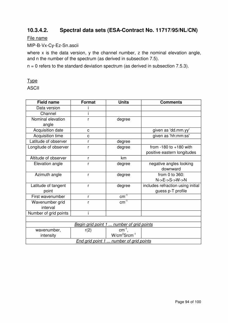
Page 94 of 100
10.3.4.2. Spectral data sets (ESA-Contract No. 11717/95/NL/CN)
File name
MIP-B-Vx-Cy-Ez-Sn.ascii
where x is the data version, y the channel number, z the nominal elevation angle,
and n the number of the spectrum (as derived in subsection 7.5).
n = 0 refers to the standard deviation spectrum (as derived in subsection 7.5.3).
Type
ASCII
Field name Format Units Comments
Data version i
Channel i
Nominal elevation
angle
r degree
Acquisition date c given as 'dd.mm.yy'
Acquisition time c given as 'hh:mm:ss'
Latitude of observer r degree
Longitude of observer r degree from -180 to +180 with
positive eastern longitudes
Altitude of observer r km
Elevation angle r degree negative angles looking
downward
Azimuth angle r degree from 0 to 360:
N->E->S->W->N
Latitude of tangent
point
r degree includes refraction using initial
guess p-T profile
First wavenumber r cm-1
Wavenumber grid
interval
r cm-1
Number of grid points i
Begin grid point 1 ... number of grid points
wavenumber,
intensity
r(2) cm-1,
W/cm2Srcm-1
End grid point 1 ... number of grid points

Page 95 of 100
10.3.4.3. Spectral data sets (ESA-Contract No. 12078/96/NL/GS)
File name
MIP-B-Vx-Cy-Ez-Sn.hdf
where x is the data version, y the channel number, z the nominal elevation angle,
and n the number of the spectrum (as derived in subsection 7.5).
n = 0 refers to the standard deviation spectrum (as derived in subsection 7.5.3).
Type
HDF
The HDF data format is used for exchange of MIPAS-B2 data between ESA and the
contractor. Further information about HDF can be found on the World Wide Web
[HDF1999].
The information content is identically to the one described in subsection 10.3.4.2.
The following source code is written in IDL, which condenses the data to the HDF-
files:
;--------------------------------------------------------------------------------
; Procedure to construct the HDF files using IDL
;--------------------------------------------------------------------------------
pro esa_hdf,filename,latitude,longitude,altitude,realelev,azimuth,lattangent
arr = read_XYfile(strmid(filename,0,21)+'.bin',time=time)
filename = strmid(filename,0,21)+'.hdf'
sd_id = HDF_SD_START(filename, /CREATE)
HDF_DFAN_ADDFDS, filename, 'Spectrum of the MIPAS-B2 Flight from Aire sur
l''Adour,1998 (c) IMK/FZK'
HDF_SD_ATTRSET, sd_id, 'Filename', filename
HDF_SD_ATTRSET, sd_id, 'Data version', strmid(filename,7,1)
HDF_SD_ATTRSET, sd_id, 'Channel', fix(strmid(filename,10,1))
HDF_SD_ATTRSET, sd_id, 'Nominal elevation angle', loat(strmid(filename,13,5))
HDF_SD_ATTRSET, sd_id, 'Acquisition date', strmid(time,5,8)
HDF_SD_ATTRSET, sd_id, 'Acquisition time', strmid(time,14,8)
HDF_SD_ATTRSET, sd_id, 'Latitude of observer', latitude
HDF_SD_ATTRSET, sd_id, 'Longitude of observer', longitude
HDF_SD_ATTRSET, sd_id, 'Altitude of observer', altitude
HDF_SD_ATTRSET, sd_id, 'Elevation angle', realelev
HDF_SD_ATTRSET, sd_id, 'Azimuth angle', azimuth
HDF_SD_ATTRSET, sd_id, 'Latitude of tangent point', lattangent
HDF_SD_ATTRSET, sd_id, 'First Wavenumber', arr[0,0]
HDF_SD_ATTRSET, sd_id, 'Wavenumber grid interval', 0.025d0
sz=size(arr)
HDF_SD_ATTRSET, sd_id, 'Number of grid points',sz(1)
if sz(0) eq 0 then return
sds_id = HDF_SD_CREATE(sd_id, 'Spectrum [Wavenumber,Intensity]', sz(1:sz(0)),
/DOUBLE)
HDF_SD_ADDDATA, sds_id, arr ;Write the data into the dataset.
HDF_SD_ENDACCESS, sds_id ;End access to any SD IDs.
HDF_SD_END, sd_id ;When finished with the file, close it with a call to
return
end

Page 96 of 100
10.3.4.4. Pressure-temperature initial guess profile (ESA-
Contract No. 11717/95/NL/CN and ESA-Contract No.
12078/96/NL/GS)
File name
MIP-B-Vx-PT
where x is the data version.
Type
ASCII
Field name Format Units Comments
Number of
atmospheric levels
i
Altitude of
atmospheric levels
r(number of
levels)
km
Pressure at levels r(number of
levels)
hPa
Temperature at levels r(number of
levels)
K

Page 97 of 100
10.4. HDF data format description of delivered data
The HDF data format has been agreed for exchange of MIPAS-B2 data between
ESA and the contractor.
General format used within HDF:
The Hierarchical Data Format (HDF) is a multi-object file format that facilitates the
transfer of various types of data between machines and operating systems. HDF is a
product of the National Center for Supercomputing Applications (NCSA). HDF is
designed to be flexible, portable, self-describing and easily extensible for future
enhancements or compatibility with other standard formats. The HDF library contains
interfaces for storing and retrieving images and multi-dimensional scientific data.
Further information about HDF can be found on the World Wide Web. The HDF
"Frequently-Asked Questions" file can be found at:
http://hdf.ncsa.uiuc.edu:8001/HDF-FAQ.html
The following source code is written in IDL, which supports HDF3_3r4, and retrieves
the metadata from the HDF-file giving information an the data and its formats stored
within this file:
pro testhdf,filename,OUTFILE=outfile
; displays Raster,SD,MSDS and Vset information about filename,
; in tabular format
F4='(A,I15)'
F5='(A14," ",A8," ",A5)'
FS='(A14," ",A8," : ",A)'
FF='(A14," ",A8," : ",F)'
FD='(A14," ",A8," : ",D)'
; Check for required number of input parameters
if n_params() lt 1 then begin
print,'usage: hdftest,filename [,OUTFILE=outfile]'
print," ARGUMENTS : filename : string name of HDF file"
print," KEYWORDS:"
print," OUTFILE : filename for output information"
print," to be written to (optional)"
print,' OUTPUTS: the HDF metadata for this file,'
print,' always to the display, and possibly'
print,' to the outfile specified'
print,"EXAMPLE: hdfinfo,'demo.hdf'"
print,'will display the HDF metadata for this file'
return
endif
; Check that it is HDF !
if hdf_ishdf(filename) ne 1 then begin
message,"File "+filename+" is not an HDF file."
endif
; Open the HDF file readonly
fileid=hdf_open(filename,/read)
print," *****BEGINNING OF HDF_INFORMATION***** "
print," FILENAME : ",filename
; Get the number of file descriptions and read them.
numdesc=hdf_number(fileid,tag=101)>0

Page 98 of 100
print,''
if numdesc eq 1 then begin
hdf_dfan_getfds,filename,desc,/first
print," FILE DESCRIPTION :"
print,' '+string(desc)
endif
; Get the number of SDSs in the file
numndg=hdf_number(fileid,tag=721)>0
numsdd=hdf_number(fileid,tag=701)>0
numsd=hdf_number(fileid,tag=702)>0
hdf_dfsd_getinfo,filename, NSDS=numsds
print,''
print,' # OF SDS : ',numsds,FORMAT=F4
sd_id=HDF_SD_START(filename,/read)
HDF_SD_FILEINFO,sd_id,nmfsds,nglobatts
; Get the number of file descriptions and read them.
print,''
print,' # OF GLOBAL ATTRIBUTES : ',nglobatts,FORMAT=F4
if nglobatts gt 0 then begin
print," ----------------------------------------"
print,'Name','Type','Value',FORMAT=F5
for i=0,nglobatts-1 do begin
HDF_SD_ATTRINFO,sd_id,i,name=n,type=t,data=d
; if (c ne 1) then print,strtrim(n),t,c,FORMAT=F4 else $
if (t eq 'STRING' ) then print,strtrim(n),t,d(0,0),FORMAT=FS else $
if (t eq 'FLOAT' ) then print,strtrim(n),t,d(0,0),FORMAT=FF else $
if (t eq 'DOUBLE' ) then print,strtrim(n),t,d(0,0),FORMAT=FD else $
print,strtrim(n),t,d(0,0),FORMAT=FI
endfor
print," ----------------------------------------"
endif
; Get the number of MFSDs in the file
print,''
print," # of MFSD : ",nmfsds,FORMAT=F4
if nmfsds gt 0 then begin
print," ----------------------------------------"
FSS='(A15," ",A4," ",A8," ",A5," ",A5)'
print,'Name','Rank','Type','Size','Value',Format=FSS
print,''
FSD='(A15," ",I4," ",A8," ",I5," ",A)'
for i=0,nmfsds-1 do begin
sds_id=HDF_SD_SELECT(sd_id,i)
HDF_SD_GETINFO,sds_id,name=n,ndims=r,type=t,natts=nats,dims=dims
HDF_SD_GETDATA,sds_id,data
if dims gt 1 then begin
print,n,r,t,dims,FORMAT=FSD
plot,data
endif else print,n,r,t,dims,string(data),FORMAT=FSD
HDF_SD_ENDACCESS,sds_id
endfor
print," ----------------------------------------"
endif
HDF_SD_END,sd_id
print," *****END OF HDF_INFORMATION***** "
hdf_close,fileid
end

Page 99 of 100
10.5. ILS calculation from Bessel coefficients
As described in subsection 6.5.1, the ILS can be directly obtained by adding
spherical Bessel functions which are weighted by a set of coefficients ci. These
Bessel coefficients are given as a polynom of second order over the wavenumber.
The printed IDL-program gives an example on how to calculate the ILS from a set of
Bessel functions without using a mathematical library for Bessel functions.
;====================================================================
; Procedure to calculate the ILS/AILS from given Bessel coefficients.
;
; (c) Olaf Trieschmann, 1998
; Forschungszentrum Karlsruhe/
; Institut für Meteorologie und Klimaforschung
;
;--------------------------------------------------------------------
;
; VARIABLES
;
; sigma0 : wavenumber for which the AILS is to be calculated
;
; KEYWORDS
;
; nhalf : number of points on each side of the center with a
; a sampling interval of 0.025cm-1
; d_grid : gridspacing
; d_resol : the nominal resolution, respectively the optical path
; Ci : Coefficients of the Modulation function; if this keyword is set
; then any value to channel and sigma0 are obsolete
;
;--------------------------------------------------------------------
; Revisions:
; 15.2.2000: Appending and reorganizing of the variables and keywords
; nhalf,channel,d_grid,d_resol
;====================================================================
function bessel_ifg, sigma0, nhalf=nhalf, d_grid=d_grid, d_resol=d_resol, Ci=Ci
if not(keyword_set(nhalf)) then nhalf = 10
; the nominal resolution, respectively the optical path
if not(keyword_set(d_resol)) then d_resol = 0.0345
; gridspacing
if not(keyword_set(d_grid)) then d_grid = 0.025
; the AILS coefficients (Channel 1)
ai0 = [-1.313E-08, 6.343E-08, -2.610E-07,8.264E-07,-1.344E-06,1.172E-06,-8.853E-07,4.417E-07]
ai1 = [1.070E-05,-8.484E-05,2.686E-04,-1.102E-03,1.778E-03,-1.525E-03,1.213E-03,-5.594E-04]
ai2 = [4.014E-02,+3.115E-02,+4.446E-01,4.020E-01,-2.177E-01,5.287E-01,-4.119E-01,1.830E-01]
if not(keyword_set(Ci)) then begin
; calculation of the coefficients vs. wavenumber
ci = dblarr(n_elements(ai0))
for i = 0,(n_elements(ai0)-1) do begin
ci[i] = ai0[i]*sigma0^2 + ai1[i]*sigma0 + ai2[i]
endfor
endif
; creation of the abscissa and ordinate vector with 2*nhalf
; elements set to zero
ils = dblarr(2*nhalf+1.0)
sigma = dblarr(2*nhalf+1.0)
; creation of the abscissa working vector of nhalf points.
; The value of the elements are set to their index
sigmatmp = (dindgen(nhalf)+1.0)*d_grid/d_resol*!DPI
zero = dblarr(nhalf)
fm = dblarr(nhalf,9)
gm = dblarr(nhalf,9)
;n=1/2
fm[*,0] = zero+1.0
gm[*,0] = zero
;n=3/2
fm[*,1] = 1.0/sigmatmp
gm[*,1] = zero+1.0
;n=5/2
fm[*,2] = 3.0/sigmatmp^2-1.0

Page 100 of 100
gm[*,2] = 3.0/sigmatmp
;n=7/2
fm[*,3] = 15.0/sigmatmp^3-6.0/sigmatmp
gm[*,3] = 15.0/sigmatmp^2-1
;n=9/2
fm[*,4] = 105.0/sigmatmp^4-45.0/sigmatmp^2+1.0
gm[*,4] = 105.0/sigmatmp^3-10.0/sigmatmp
;n=11/2
fm[*,5] = (945.0/sigmatmp^3-420.0/sigmatmp^1)/sigmatmp^2+15.0/sigmatmp
gm[*,5] = (945.0/sigmatmp^2-105.0)/sigmatmp^2+1.0
;n=13/2
fm[*,6] = (10395.0/sigmatmp^3-4725.0/sigmatmp^1)/sigmatmp^3+210.0/sigmatmp^2-1.0
gm[*,6] = (10395.0/sigmatmp^3-1260.0/sigmatmp^1)/sigmatmp^2+21.0/sigmatmp
;n=15/2
fm[*,7] = ((135135.0/sigmatmp^3-62370.0/sigmatmp^1)/sigmatmp^2+3150.0/sigmatmp^1)/sigmatmp^2-28.0/sigmatmp
gm[*,7] = (135135.0/sigmatmp^4-17325.0/sigmatmp^2)/sigmatmp^2+378.0/sigmatmp^2-1.0
;n=17/2
fm[*,8] = (2027025.0/sigmatmp^4-945945.0/sigmatmp^2)/sigmatmp^4+51975.0/sigmatmp^4-630.0/sigmatmp^2+1.0
gm[*,8] = (2027025.0/sigmatmp^4-270270.0/sigmatmp^2)/sigmatmp^3+6930.0/sigmatmp^3-36.0/sigmatmp
; the tabulated Gammafunction: [GAMMA(1)..GAMMA(8)]
gamm = [+1.000E+00,+1.000E+00,+2.000E+00,+6.000E+00,+2.400E+01,+1.200E+2, $
+7.20E+2,+5.040E+3,+4.0320E+4,+3.62880E+5]
norm = [1.0, 2.0/3.0, 8.0/15.0, 48.0/105.0, 384.0/945.0, 3840.0/10395.0, 46080.0/135135.0, $
645120.0/2027025d0, 10321920d0/34459425d0]
for i = ((n_elements(ci)-1) < 8),0, -1 do begin
a = gamm[i] * 2d0^(-1) * (fm[*,i]*sin(sigmatmp) - gm[*,i]*cos(sigmatmp))
a = ci[i] * a
ils[nhalf+1:2*nhalf] = 2d0*(ils[nhalf+1:2*nhalf] + a)/sigmatmp
endfor
ils[0:nhalf-1] = reverse(ils[nhalf+1:2*nhalf])
ils[nhalf] = total(norm[0:(n_elements(ci)-1)]*ci)
; scaling of the wavenumber axis to the nominal resolution
sigma[nhalf+1:2*nhalf] = sigmatmp*d_resol/!DPI
sigma[0:nhalf-1] = -reverse(sigma[nhalf+1:2*nhalf])
for i = 0,5 do begin
print,sigma[nhalf+i],ils[nhalf+i]
endfor
return,[[sigma],[ils]]
end


![Validation of MIPAS ClONO measurements1].pdf · the IMK (Institut fur Meteorologie und Klimaforschung)¨ science-oriented data processor from MIPAS/Envisat (Michelson Interferometer](https://img.pdfslide.us/doc/110x75/5e65f881b3630f7a126ce2a9/validation-of-mipas-clono-measurements-1pdf-the-imk-institut-fur-meteorologie.jpg)