Embed Size (px)
Citation preview
;" iC FILE , EVALUATION, MAINTENANCE, AND
REHABILITATION RESEARCH PROGRAM
jin iTECHNICAL REPORT REMR-GT-11
LEVEE UNDERSEEPAGE ANALYSIS FORSPECIAL FOUNDATION CONDITIONS
by
,Ort Thomas F. Wolff
Michigan State University
oC)
September 1989
Final Report
Approved For Public Release: Distribution Unlimited
Prepared for DEPARTMENT. OF THE ARMYUS Army Corps of EngineersWashington, DC 20314-1000
Under Contract No. DACW39-87-K-0041Civil Works Work Unit 32274
Monitored by Geotechnical Laboratory"US Army Engineer Waterways Experiment Station
3909 Halls Ferry Road, Vicksburg, Mississippi 39180-6199
The following two letters used as part of the number designating technical
reports of research published under the Repair, Evaluation, Maintenance, and
Rehabilitation (REMR) Research Program identify the problem area under which
the report was prepared:
Problem Area- . Problem Area
CS Concrete and Steel Structures EM Electrical and Mechanical
CT Ceotechnical El Environmental Impacts
HY Hydraulics OM Operations Management
CO Coastal
Destroy this report when no longer needed. Do notreturn it to the originator.
The findings in this report are not to be construed as anofficial Department of the Army position unless so
designated by other authorized documents.
The contents of this report are not to be used foradvertising, publication, or promoticnal purposes.Citation of trade names does not constitute anofficial endorsement or approval of the use of such
commercial products.
COVER PHOTOS:
TOP - Schematic of levee underseepage.SECOND - Expedient measures for control of high water.THIRD - Sand boll ringed with sandbags to control adverse effects of
underseepage.BOTTOM - Levee erosion due to a combination of underseepage and through
seepage.
UnclassifiedSECURITY CLASSIFICATION OF THIS PAGE
Form ApprovedREPORT DOCUMENTATION PAGE OMB No. 0704-0188
Ia. REPORT SECURITY CLASSiFiCATION 1b RESTRICT;VE MARKNGSUnclassified
2a. SECURITY CLASSIFICATION AUTHORITi 3 DISTRIBUTION, AVAILABILITY OF REPORTApproved for public release; distribution
2b. OECLASSIFICATION /DOWNGRADING SCHEDULE unlimited.
4 PERFORMING ORGANiZAT.ON REPORT NUMBER(S( 5 MONiTORING ORGAN,ZATION REPORT NuMBER(S)
Technical Report REMR-GT-11
6a. NAME OF PERFORMING ORGANIZATION 6b. OFFICE SYMBOL 7a. NAME OF MONITORING ORGANI"ATION(If applicable) USAEWES .-
Michigan State University Geotechnical Laboratory
6c. ADDRESS (City, State, and ZIPCode) 7b. ADDRESS (City, State, and ZIP Code)
Division of Engineering Research 3909 Halls Ferry RoadEast Lansing, MI 48824-1212 Vicksburg, MS 39180-6199
8.. NAME OF FUNDING/SPONSORING Bb. OFFICE SYMBOL 9. PROCUREMENT INSTRUMENT IDENTIFICATION NUMBERORGANIZATION (If applicable)
US Army Corps of Engineers Contract No. DACW39-87-K-0041
8c. ADDRESS (City, State, an, ZIP Code) 10 SOURCE OF FUNCiNG NUMBERS
PROGRAM PROJECT TASK WORK UNIT
Washington, DC 20314-1000 ELEMENT NO. NO. NO. CCESSION NO.
W a s h i n g t o n ,_C_03 1 -1 0 0 0I I 3 2 2 7 4
11. TITLE (Include Security Classification)
Levee Underseepage Analysis for Special Foundation Conditions
12. PERSONAL AUTHOR(S)Wolff, Thomas F.13a. TYPE OF REPORT 13b. TIME COVFQFD 14 DATE OF REPORT (Year, Month, Day) 15. PAGE COUNTFinal report FROM Mar 87 TO Se 87 September 1989 152
16. SUPPLEMENTARY NOTATION
See reverse
17. COSATi CODES 18. SUBJECT TERMS (Continue on reverse if necessary and identfy by block number)
FIELD GROUP SUB-GROUP
See reverse.
19. ABSRACT (Continue on reverse if necessary and identify by block number)
-This report describes a research study in which techniques were developed for
prediction of underseepage conditions for special cases of levee and foundation geometry.The differential equations for levee underseepage were derived and programmed in finitedifference form for three special cases of boundary conditions. The developed programsallow analyses that are not restricted to the boundary conditiuris assumed in the conven-tional, closed form solution, i.e., two foundation layers of uniform thickness withhorizontal boundaries.
The three special cases of foundation conditions that can be analyzed are as follow:
a. Foundations consisting of three layers of uniform thickness with horizontalboundaries and differing horizontal and vertical permeability in each layer.
(Continued)
20. DISTRIBUTION/AVAILABILITY OF ABSTRACT 21 ABSTRACT SECURITY CLASSIFICATION0 UNCLASSIFIEO/UNLIMITED C3 SAME AS RPT C3 DTIC USERS Unclassified
22a. NAME OF RESPONSIBLE INDIVIDUAL 22b TELEPHONE (Include Area Code) 2c. OFFICE SYMBOL
DO Form 1473, JUN 86 Previous editions are obsolete. SECUR;TY CLASS;FICATION OF THIS PAGE
Unclassified
Unc assi iedSUCUmeTY CLA"SIF. CATION OF TMIS PGSe
16. SUPPLLENTARY NOTATION (Continued).
A report of the Geotechnical problem area of the Repair, Evaluation, Maintenance, andRehabilitation (REMR) Research Programs. Available from the National Technical InformationService, 5285 Port Royal Road, Springfield, VA 22161.
18. SUBJECT TERMS (Continued).
Analyses Numerical methodsFoundations PermeabilityGeometry evaluation RehabilitationIrregular boundaries UnderseepageLevee-
19. ABSTRACT (Continued).
' b. Foundations consisting of two layers of nonuniform thickness with irregularboundaries.
c. Levee reaches where the levee alignment bends or forms a corner. Capabilities ofthe techniques and programs are demonstrated by comparing theoretical solutions
to observed performance at eight field locations where piezometric data areavailable. At each location, the field permeability ratio was estimated byvarying program input and seeking a match between the program output and actualobserved performance. "L
SECURITY CLASSIFICATION OF THIS P&G
PREFACE
This study reported herein was performed during the period 18 March 1987
through 30 September 1987 under Contract No. DACW39-87-K-0041 as a research
need of Work Unit 32274, "Rehabilitation Alternatives to Control Adverse
Effects of Levee Underseepage," of the Repair, Evaluation, Maintenance, and
Rehabilitation (REMR) Research Program being conducted by the US Army Engineer
Waterways Experiment Station (WES).
This report was prepared by Dr. Thomas F. Wolff of Michigan State
University. The study addresses the prediction of underseepage conditions for
special cases of levee and foundation geometry that may not be adequately
modeled by traditional procedures. Dr. Wolff was assisted by
Messrs. Magdal N. Haji, Hassan Al-Moussawi, Ali F. A. Rassoul, Fritz Klingler,
and Shawn Reed.
The study was under the direct supervision of Mr. G. Britt Mitchell, the
Problem Area Leader. Mr. Hugh M. Taylor, Jr., was Principal Investigator and
Contracting Officer's Representative, Soil Mechanics Division (SMD), during
the conduct and publication of the work. General supervision was provided by
Mr. Clifford L. McAnear, Chief, SMD, and Dr. William F. Marcuson III, Chief,
GL.
Data and technical support for the study were provided by
Messrs. George Mech, Sibte A. Zaidi and Donald Baumann of Rock Island Dis-
trict; Bruce H. Moore, George J. Postol, and Patrick J. Conroy of the
St. Louis District; Joseph Keithly and John Monroe of the Memphis District;
and Bobby Fleming and Wayne Forrest of the Vicksburg District. Partial fund-
ing was provided by the Rock Island and Vicksburg Districts.
The Directorate of Research and Development Coordinator for REMR in
Headquarters, US Army Corps of Engineers (HQUSACE), was Mr. Jesse A. Pfeiffer,
Jr. Members of the REMR Overview Committee in HQUSACE were Mr. James E. Crews
and Dr. Tony C. Liu. Mr. Arthur H. Walz was Technical Monitor. The WES REMR
Program Manager was Mr. William F. McCleese, WES.
Commander and Director of WES during the preparation of this report
was COL Larry B. Fulton, EN. Dr. Robert W. Whalin was Technical Director.
• • , .a I l I l
CONTENTS
PREFACE...................................................................
LIST OF TABLES. ......................................................... 4
LIST O FIGURES ........................................................... 4
CONVERSION FACTORS, NON-SI TO SI (METRIC)UNITS OF MEASUREMENT .................................................... 7
PART I: INTRODUCTION ................................................... 8
Background, Purpose, and Scope ...................................... 8
Previoup Studies ..................................................... 10Back-Calculation of Parameters ...................................... 12
PART II: SPECIAL CASES OF FOUNDATION CONDITIONS ...................... 15
Foundations Characterized by Three Layers ......................... 15
Foundations Characterized by Two Layers of Irregular Shape ........ 17Angles of "Corners" in Levee Alignment .............................. 1
PART III: SELECTION OF LEVEE REACHES FOR STUDY ........................ 20
Selection Criteria ................................................... 20
Selected Reaches ..................................................... 20
PART IV: FOUNDATIONS CHARACTERIZED BY THREE LAYERS ................... 23
Numerical Modeling Technique ........................................ 23Effect of Moderately Pervious Middle Stratum ...................... 23
Actual Versus Predicted Performance ................................. 29
PART V: FOUNDATIONS CHARACTERIZED BY TWO LAYERS OF IRREGULAR
SHAPE .......................................................... 46
Numerical Modeling Technique ........................................ 46Effect of Nonuniform Layer Thickness ................................ 46
Actual Versus Predicted Performance ................................. 49
PART VI: ANGLES OR "CORNERS" IN LEVEE ALIGNMENT ...................... 73
Numerical Modeling Technique ........................................ 73
Effect of Levee Curvature ............................................ 73Actual Versus Predicted Performance ................................. 78
PART VII: CONCLUSIONS AND RECOMMENDATIONS ............................... 87
Conclusions .......................................................... 87Recommendations ...................................................... 90
REFERENCES ................................................................ 91
APPENDIX A: COMPUTER PROGRAM LEVEE3L: UNDERSEEPAGE ANALYSIS FORFOUNDATIONS CHARACTERIZED BY THREE LAYERS ................. Al
APPENDIX B: COMPUTER PROGRAM LEVEEIRR: UNDERSEEPAGE ANALYSIS FORFOUNDATIONS CHARACTERIZED BY TWO LAYERS OF IRREGULARSHAPE ........................................................ BI
2

Page
APPENDIX C: COMPUTER PROGRAM LEVEECOR: U1NDERSEEPAGE ANALYSIS ATANGLES OR "CORNERS" IN LEVEE ALIGNMENT ....................... Cl
APPENDIX D: COMPARISON OF PROGRAMS...................................... Dl
APPENDIX E: NOTATION..................................................... El
COMPUTER DISKS ATTACHED
3
LIST OF TABLES
TableNo. Page
1 Parameters Used for Analyses, Rock Island District, Sny
Island, Range F ................................................... 322 Parameters Used For Analyses, Vicksburg District, Eutaw, Miss,
Line D ............................................................ 393 Parameters Used for Analyses, Rock Island District, Hunt,
Range B ........................................................... 514 Parameters Used for Analyses, Memphis District, Commerce, Miss,
Line H ............................................................ 555 Parameters Used for Analyses, Memphis District, Stovall, Miss,
Line B ............................................................ 626 Parameters Used for Analyses, Vicksburg District, Bolivar, Miss,
Range D ........................................................... 687 Parameters Used for Analyses, St. Louis District, Degognia,
Station 260-290 ................................................... 818 Parameters Used for Analyses, St. Louis District, East Cape,
Station 94 ........................................................ 84
LIST OF FIGURES
Figure
No. Page
1 Bennett's analysis .................................................. 112 TM 3-424 solutions for finite foundation lengths ................. 133 Example of the three-layer foundation ............................ 16
4 Example of an irregular foundation ............................... 185 Example of angle in levee alignment ................................ 19
6 Locations of analyzed levee reaches ................................ 217 Variables and grid used by Program LEVEE3L ....................... 24
8 Program LEVEE3L, flow at interior node ............................. 259 Gradient, i, versus permeability of middle stratum ............... 26
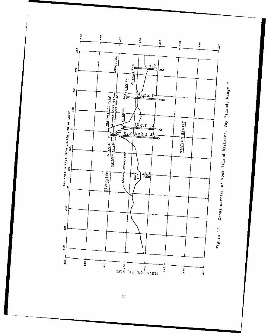
10 Gradient versus thickness of middle stratum ...................... 2711 Gradient versus thickness of top blanket ......................... 2812 Cross section of Rock Island District, Sny Island, Range F ....... 3113 Results of analyses, Rock Island District, Sny Island, Range F,
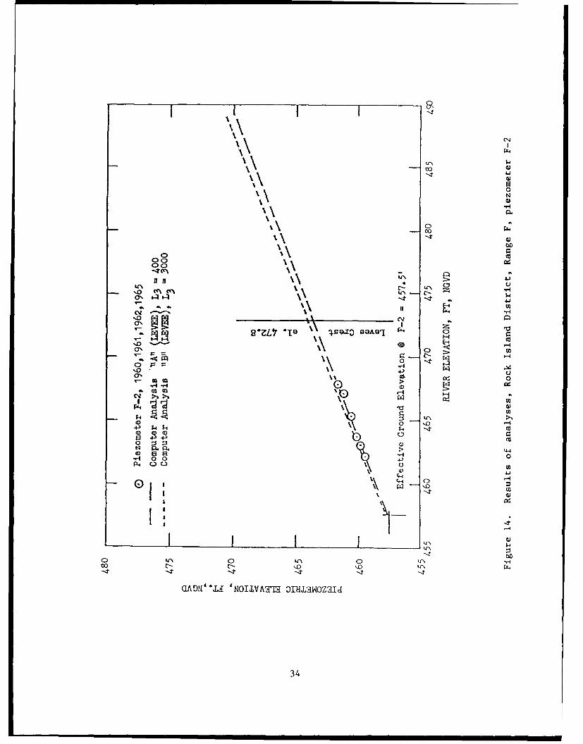
piezometer F-i .................................................... 3314 Results of analyses, Rock Island District, Sny Island, Range F,
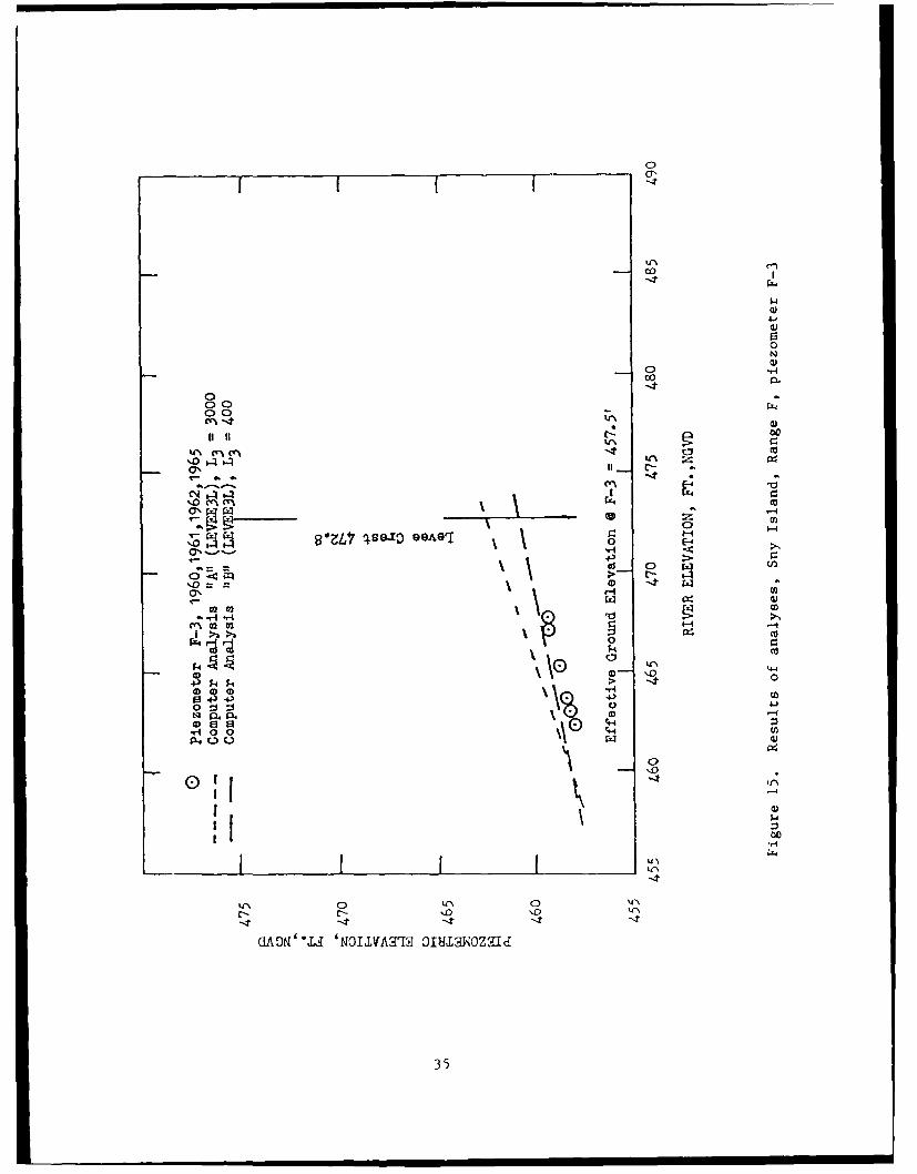
piezometer F-2 .................................................... 3415 Results of analyses, Rock Island District, Sny Island, Range F,
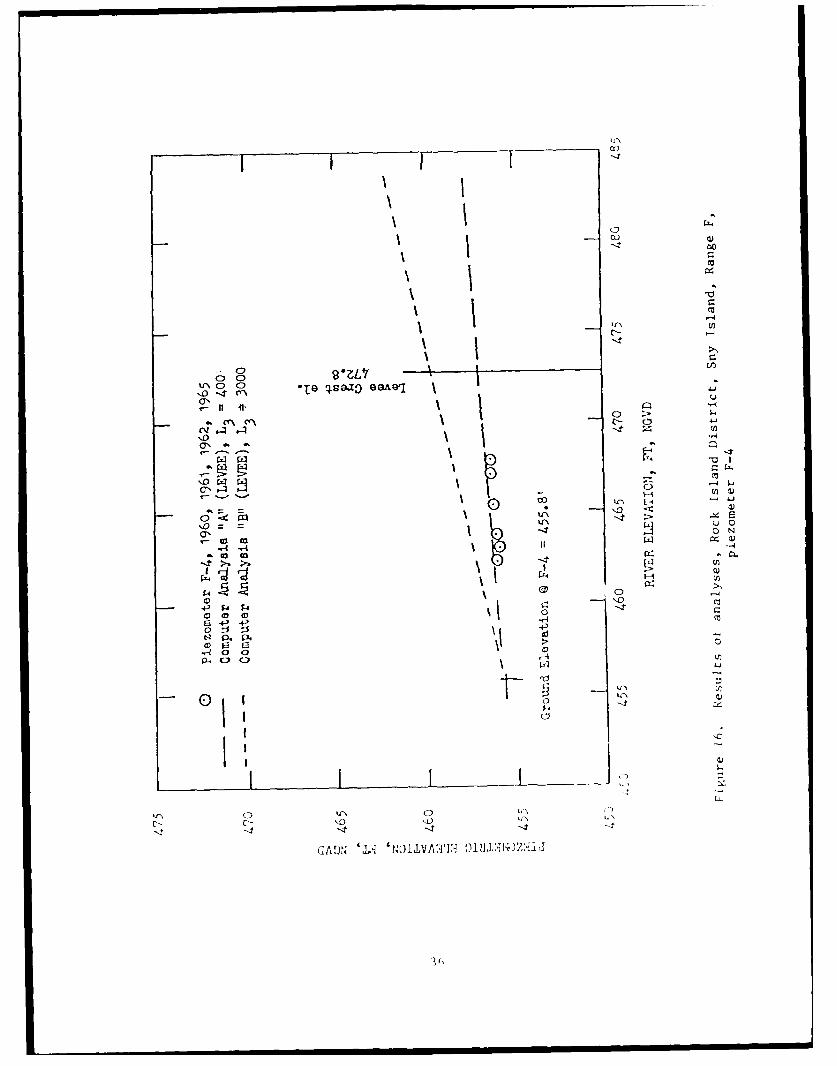
piezometer F-3 .................................................... 3516 Results of analyses, Rock Island District, Sny Island, Range F,
piezometer F-4 .................................................... 3617 Cross section of Vicksburg District, Eutaw, Miss, Line D ......... 38
18 Results of analyses, Vicksburg District, Eutaw, Miss, Line D,piezometers D-1 and D-2 ........................................... 40
19 Results of analyses, Vicksburg District, Eutaw, Miss, Line D,piezometers D-3 and D-4 ........................................... 41
4
LIST OF FIGURES (Continued)
Figure
No. Page
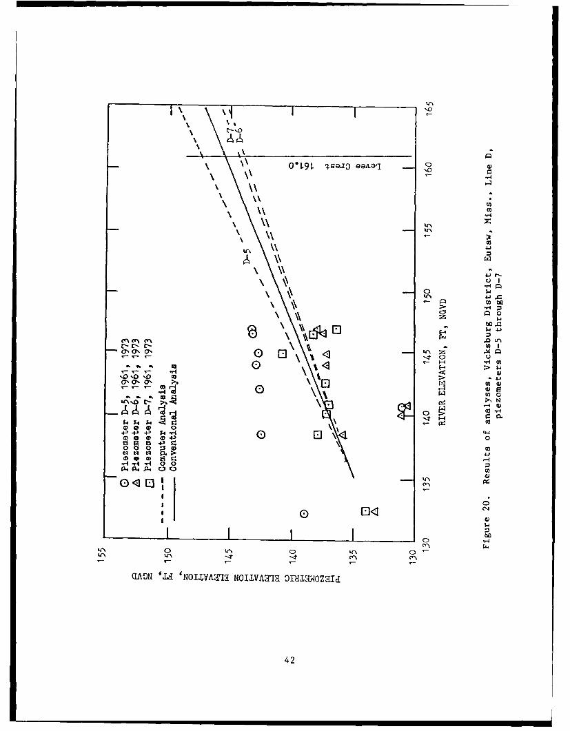
20 Results of analyses, Vicksburg District, Eutaw, Miss, Line D,piezometers D-5 through D-7 ...................................... 42
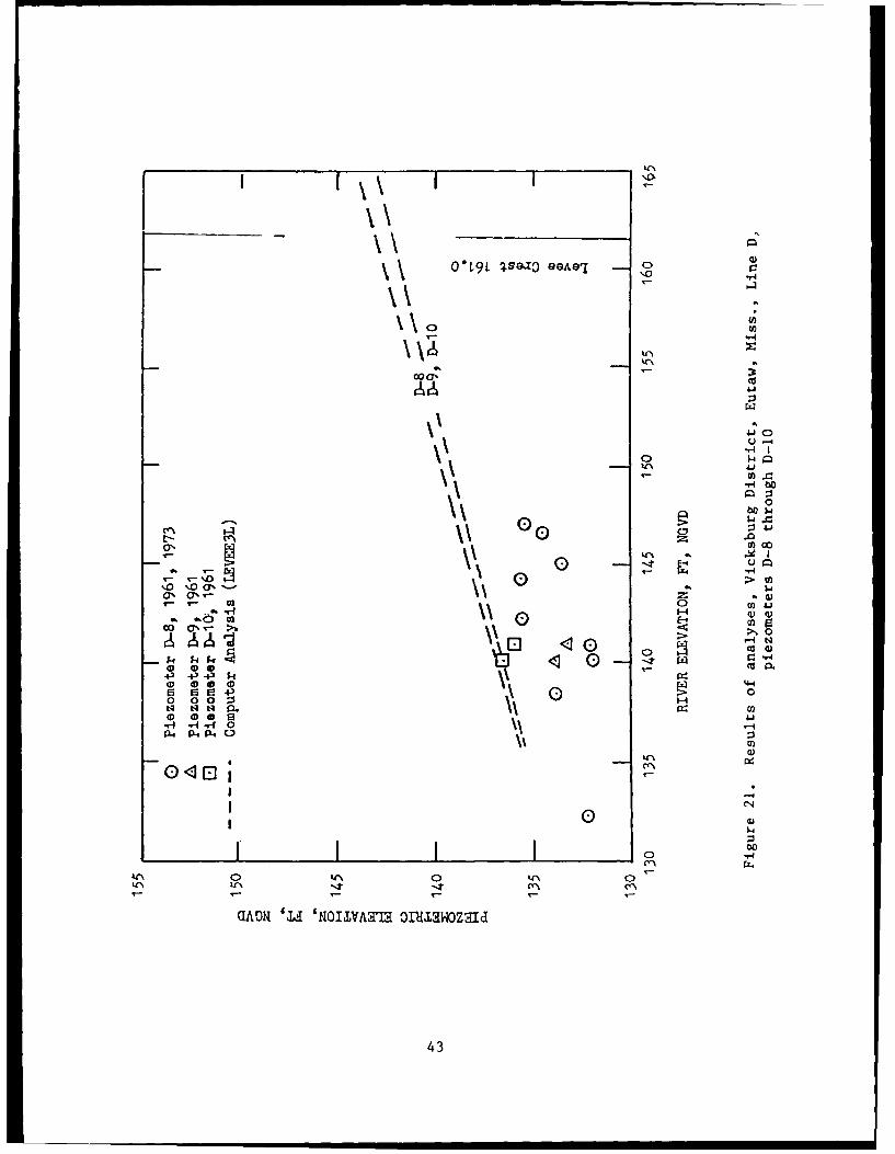
21 Results of analyses, Vicksburg District, Eutaw, Miss, Line D,piezometers D-8 through D-1O ................................... 43
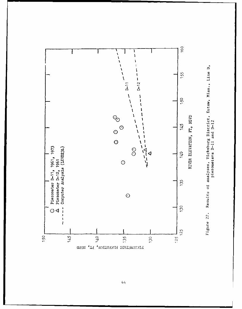
22 Results of analyses, Vicksburg District, Eutaw, Miss, Line D,
piezometers D-11 and D-12 ........................................ 4423 Analysis technique used in LEVEEIRR .............................. 4724 Effect of landside ditch ........................................... 4825 Actual and modeled cross sections of Rock Island District, Hunt,
Range "B"........................................................ 5026 Results of analyses, Rock Island District, Hunt, Range "B" ........ 5227 Actual and modeled cross sections of Memphis District,
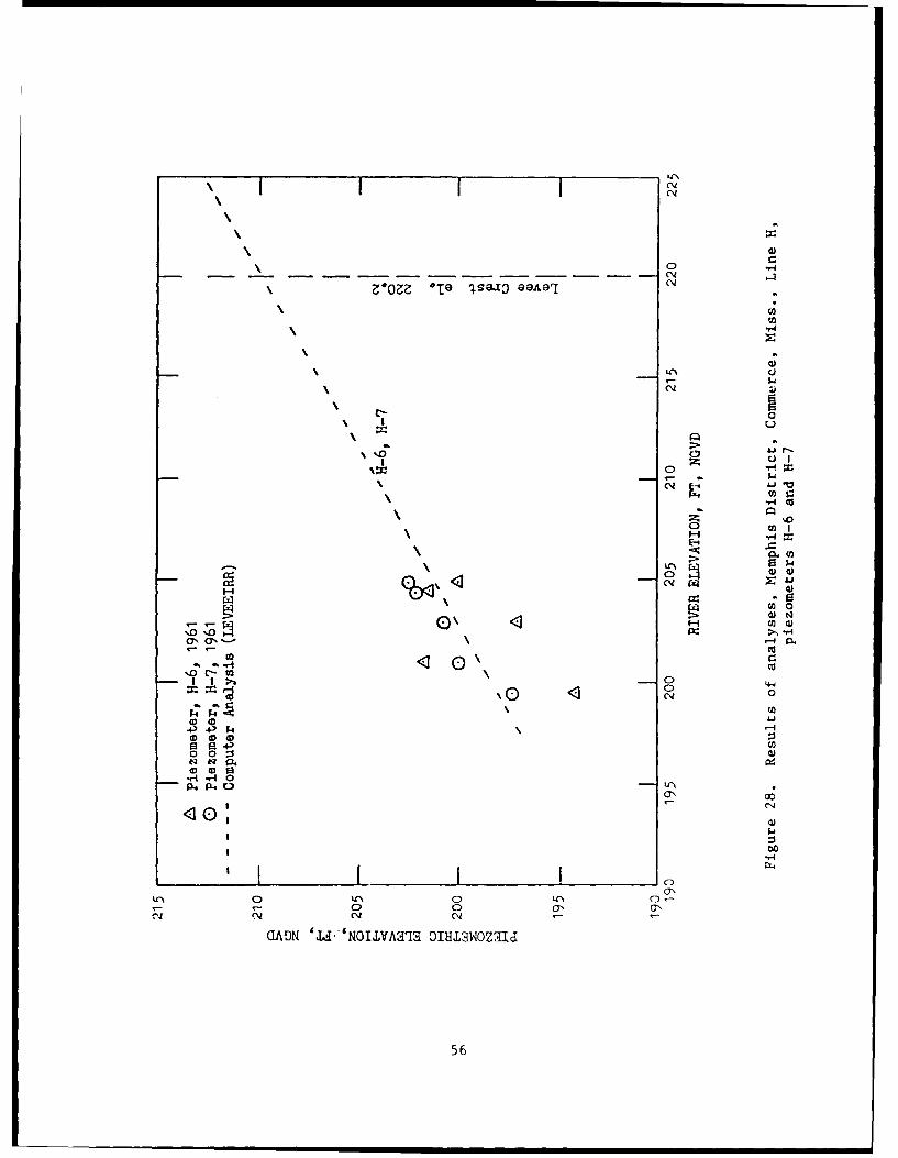
Commerce, Miss, Line H ........................................... 5428 Results of analyses, Memphis District, Commerce, Miss, Line H,
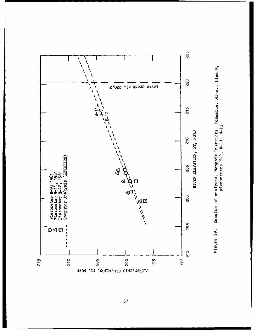
piezometers H-6 and H-7 .......................................... 5629 Results of analyses, Memphis District, Commerce, Miss, Line H,
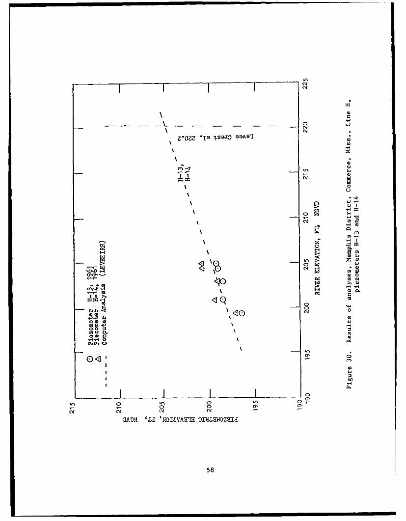
piezometers H-9, H-li and H-12 ................................. 5730 Results of analyses, Memphis District, Commerce, Miss, Line H,
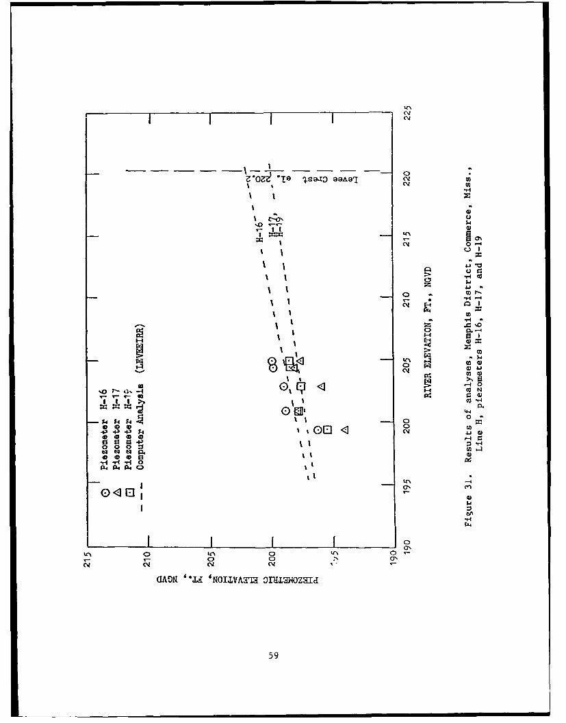
piezometers H-13 and H-14 ........................................ 5831 Results of analyses, Memphis District, Commerce, Miss, Line H,
piezometers H-16, H-17, and H-19 ............................... 5932 Results of analyses, Memphis District, Commerce, Miss, Line H,
piezometers H-20 through H-22 .................................... 6033 Actual and modeled cross sections of Memphis District,
Stovall, Miss, Line B ............................................ 6134 Results of analyses, Memphis District, Stovall, Miss, Line B
piezometers E-11 and E-13 ........................................ 6335 Results of analyses, Memphis District, Stovall, Miss, Line B
piezometers E-14 and E-15 ........................................ 6436 Results of analyses, Memphis District, Stovall, Miss, Line B,
picze ters F-16 ?n1 E-17 ... .................................. 6537 Actual and modeled cross sections of Vicksburg District,
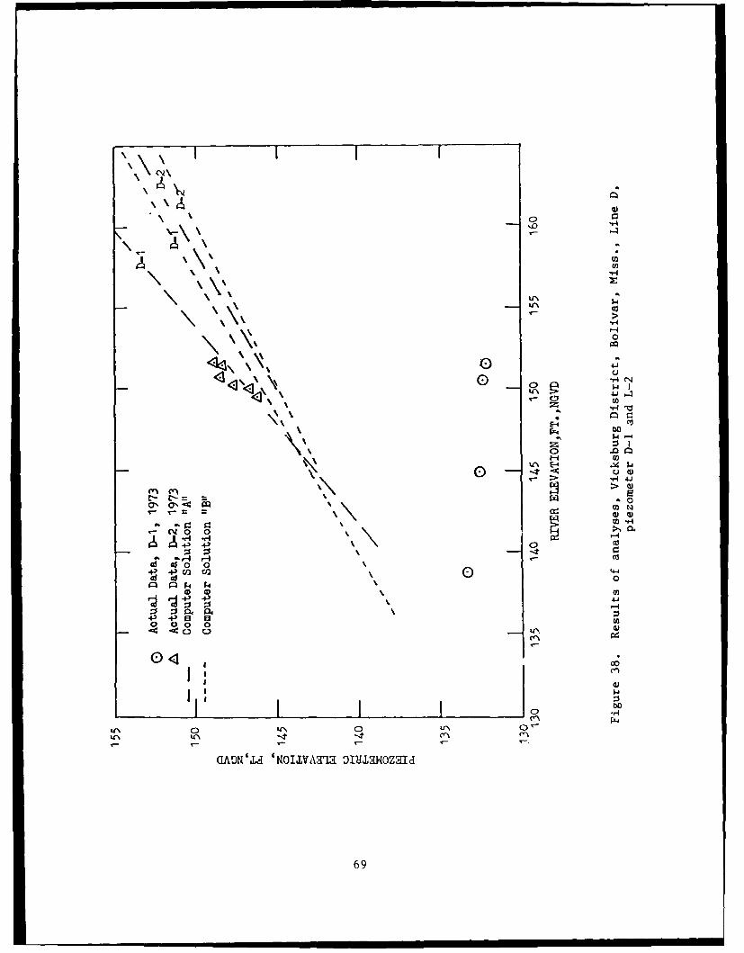
Bolivar, Miss, Line D ............................................ 6738 Results of analyses, Vicksburg District, Bolivar, Miss, Line D,
piezometers D-1 and D-2 .......................................... 6939 Results of analyses, Vicksburg District, Bolivar, Miss, Line D,
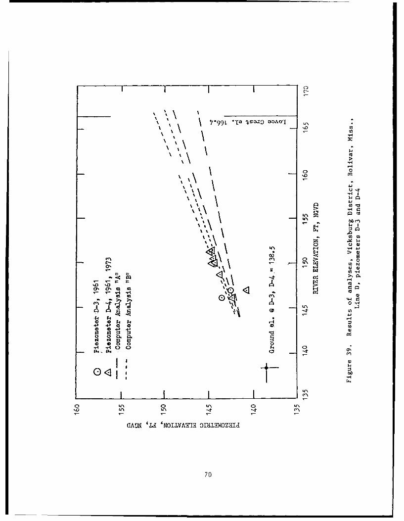
piezometers D-3 and D-4 .......................................... 7040 Results of analyses, Vicksburg District, Bolivar, Miss, Line 0,
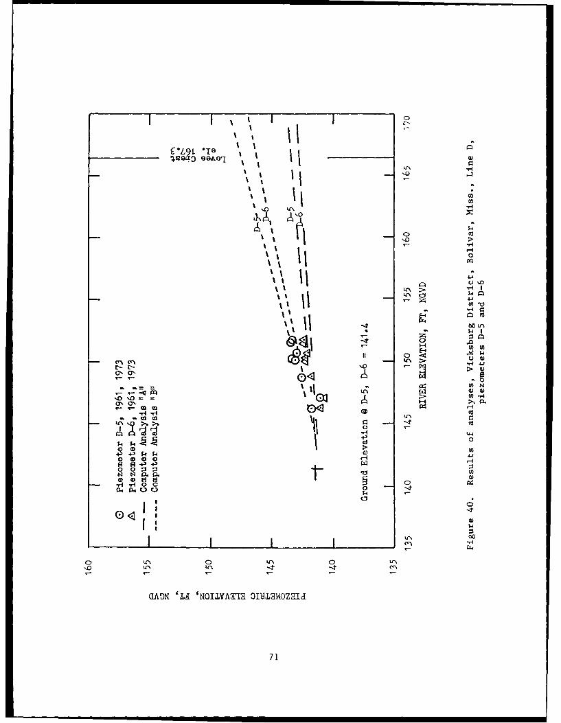
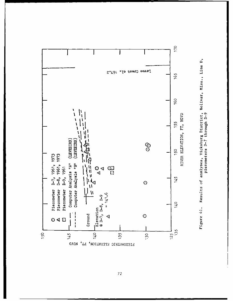
piezometers D-5 and D-6 .......................................... 7141 Results of analyses, Vicksburg District, Bolivar, Miss, Line D,
piezometers D-7 through D-9 ...................................... 7242 Levee geometry used by program LEVEECOR .......................... 7443 Grid generated by program LEVEECOR ............................... 7544 Flow at an interior node, program LEVEECOR ....................... 76
45 Results of parametric study using LEVEECOR ....................... 7746 Plan and profile of St. Louis District, Degognia,
Station 260-290 ................................................... 7
5
LIST OF FIGURES (Concluded)
Figure
No. Page
47 Results of analyses, St. Louis District, Degognia,
Station 260-290 ................................................... 8248 Plan and profile of St. Louis District, East Cape, SLdtion 94 .... 8349 Results of analyses, St. Louis District, East Cape,
Station 94 ........................................................ 85Al Example input file, program LEVEE3L .............................. A2A2 Definition of variables, program LEVEE3L ......................... A4A3 Example run for program LEVEE3L .................................... A5A4 Example output file, program LEVEE3L .............. .............. A6A5 Listing of program LEVEE3L .......................................... A8BI Example input file, program LEVEEIRR ............................. B2B2 Definition of variables, program LEVEETRR ........................ B4B3 Example run for program LEVEEIRR ................................... B5B4 Example output file, program LEVEEIRR ............................ B6B5 Listing of program LEVEEIRR ......................................... B8Cl Example input file, program LEVEECOR ............................. C2C2 Definition of variables, program LEVEECOR ........................ C4
C3 Example of run for program LEVEECOR .............................. C5C4 Example output file, program LEVEECOR ............................ C7
C5 Listing of program LEVEECOR ......................................... C12
D1 Comparison of results for example problem ......................... D2
6
• ' I i II
LEVEE UNDERSEEPAGE ANALYSIS FOR SPECIAL
FOUNDATION CONDITIONS
PART I: INTRODUCTION
Background, Purpose, and Scope
1. A Repair, Evaluation, Maintenance, and Rehabilitation (REMR) Levee
Underseepage Workshop was held at the US Army Engineer Waterways Experiment
Station (WES) on 19 April 1984 to establish research needs related to control
of levee underseepage. Representatives from the Rock Island, St. Louis,
Memphis, and Vicksburg Corps of Engineers (CE) Districts attended the work-
shop. One of the research tasks established was comparing predicted levee
underseepage conditions to observed performance. In September 1986, a criti-
cal review of underseepage analysis procedures was prepared by this author
(Wolff 1986) under an Interagency Personnel Agreement with the WES Geotechni-
cal Laboratory. The workshop and the critical review both indicated that
levee and foundation geometry may significantly affect seepage conditions, and
the method of modeling geometry in analysis may affect performance
predictions.
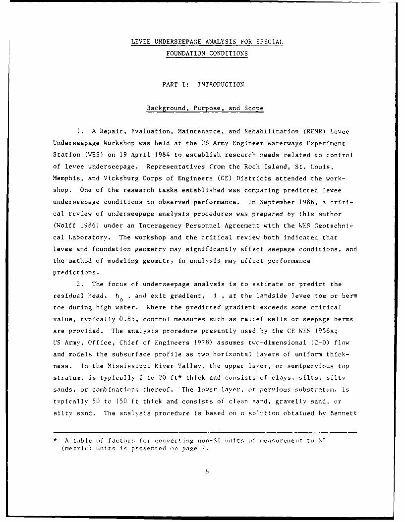
2. The focus of underseepage analysis is to estimate or predict the
residual head, h , and exit gradient, i , at the landside levee toe or berm0
toe during high water. Where the predicted gradient exceeds some critical
value, typically 0.85, control measures such as relief wells or seepage berms
are provided. The analysis procedure presently used by the CE WES 1956a;
US Army, Office, Chief of Engineers 1978) assumes two-dimensional (2-D) flow
and models the subsurface profile as two horizontal layers of uniform thick-
ness. In the Mississippi River Valley, the upper layer, or semipervious top
stratum, is typically 2 to 20 ft* thick and consists of clays, silts, silty
sands, or combinations thereof. The lower layer, or pervious substratum, is
typically 50 to 150 ft thick and consists of clean sand, gravelly sand, or
silty sand. The analysis procedure is based on a solution obtained by Bennett
* A table of factors for converting non-SI inits of measurement to $1
(metric) units is p-esented on page 7.
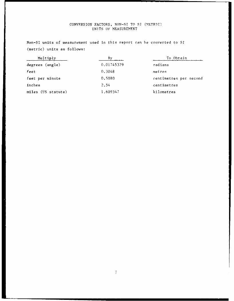
CONVERSION FACTORS, NON-SI TO SI (METRIC)
UNITS OF MEASUREMENT
Non-SI units of measurement used in this report can be converted to ST
(metric) units as follows:
Multiply By To Obtain
degrees (angle) 0.01745329 radians
feet 0.3048 metres
feet per minute 0.5080 centimetres per second
inches 2.54 centimetres
miles (US statute) 1.609347 kilometres
6. Use of the developed computer programs is described in Appendices A,
B, and C; the programs LEVEE3L, LEVEEIRR, LEVEECOR and the conventional method
are compared in Appendix D; the notation is documented in Appendix E.
Previous Studies
Infinitely long foundations
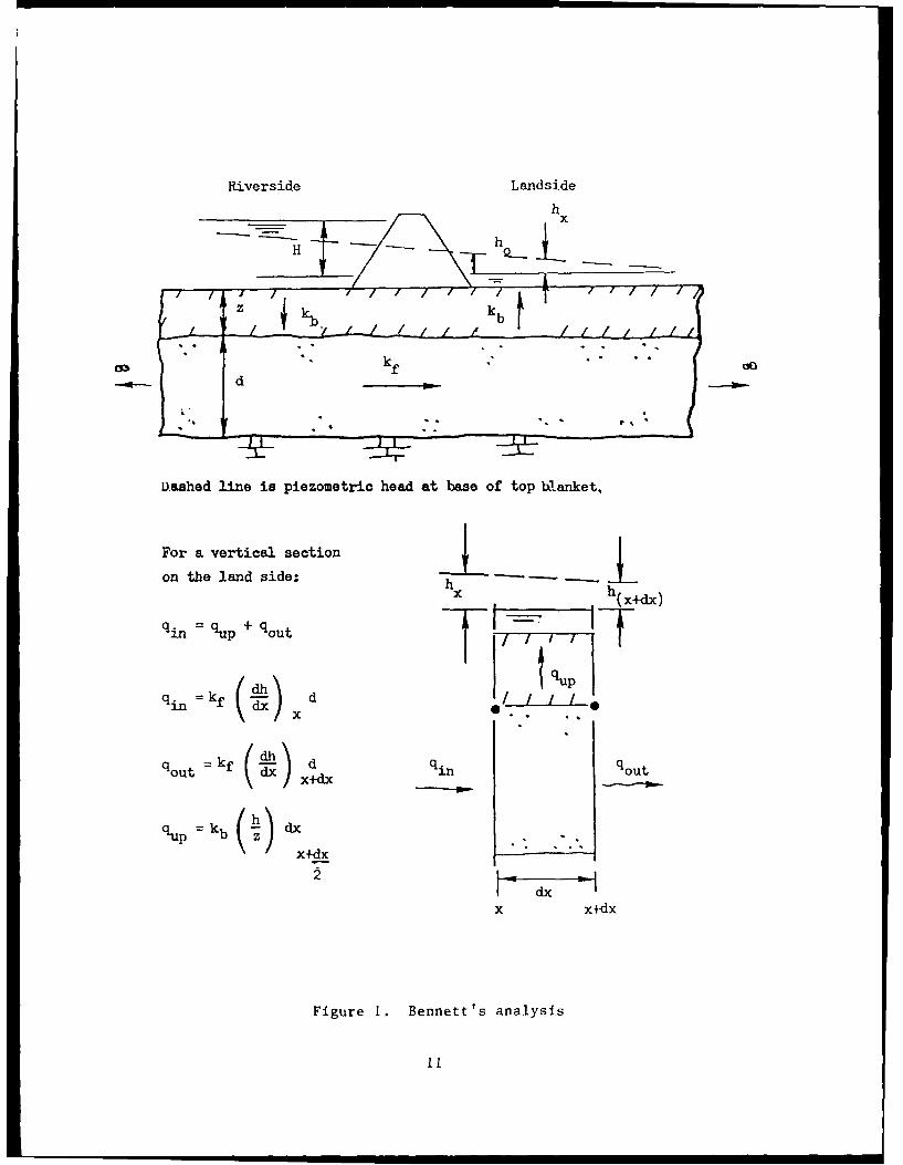
7. Bennett (1946) derived a solution for steady-state flow through a
two-layer foundation consisting of a semipervious top blanket of thickness z
overlying a pervious substratum of thickness d , both of infinite lateral
extent. In Bennett's analysis, flow is assumed downward vertical in the
riverside top blanket, landward horizontal in the substratum, and upward ver-
tical in the landside top blanket. Bennett stated that the substratum must be
at least 10 times as pervious as the top blanket for these assumptions to be
reasonable; this is almost always the case for levees in the Mississippi
Valley. Bennett's analysis is summarized in Figure 1. To calculate the
residual head, h , at the landside levee toe where the foundations layers0
are of infinite length, the pervious substratum and semi pervious top blanket
are replaced by finite "effective" lengths of pervious substratum and imper-
vious top stratum. These effective lengths are designated xI on the river-
side and x3 on the landside and are a function of the thicknesses and
permeabilities of the two materials. The base width of the levee is desig-
nated x2 . With the top stratum now impervious, the head in the substratum
varies linearly with distance, and the head at the levee toe, h , can be0
found by simple interpolation:
Hx3
0 x I + x2 + x3
where H is the net head on the levee (difference between river stage and
landside grounA or tailwater).
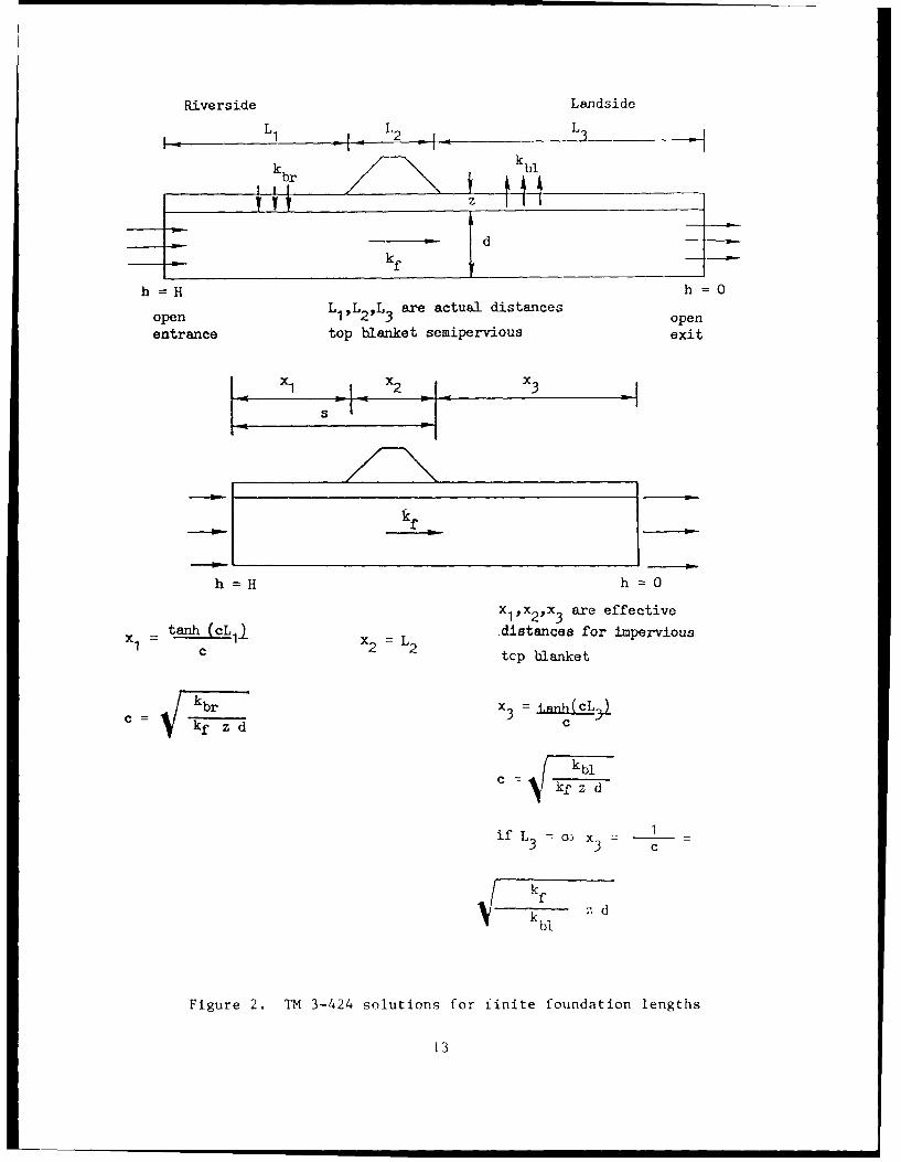
Foundations of finite length
8. Solutions for effective entrance and exit distances for finite
foundation lengths were presented by Bennett and extended and summarized in
Technical Memorandum (TM 3-424 (WES 1964)). The semipervious top blanket and
pervious substratum extend for distances of L riverward of the riverside
10
• n |10

(1946), which was extended and summarized in WES Technical Memorandum 3-424
(WES 1956a). It is referred to herein as the "conventional analysis."
Although actual foundation conditions may be highly irregular, the conven-
tional analysis requires the foundation geometry to be transformed into an
"equivalent" system of two horizontal layers of uniform thickness. Develop-
ment of the equivalent foundation may involve changing both the thickness and
permeability of the top blanket. As this transformation process can be highly
subjective, performance predictions for irregular foundation conditions are
often difficult to make and are unreliable.
3. The "conventional analysis" assumptions allow a closed-form solution
to the differential equation for the piezometric head at the interface between
the top blanket and the substratum. The residual head and gradient could
readily be calculated using 1950's techniques such as slide rules and charts.
Digital computers and numerical methods now allow solution of the flow
equation for very complex conditions. Finite element programs are available
that can model any conceivable seepage problem (e.g. Tracy 1973); however, they
are seldom used for levee underseepage analysis because the effort required
for problem description and coding is usually undesirable for routine
calculations. For levee underseepage problems, an analysis technique is
desired wherein the heads and gradients can be obtained as a function of
relatively few parameters, facilitating repetitive calculations for numerous
foundation sections along the length of a levee.
4. The purpose of this research was to develop analysis procedures that
are not constrained by some of the assumptions in the conventional procedure.
A second purpose was to investigate whether improved performance predictions
could be made using the developed procedures. As part of the research, three
computer programs were developed to perform underseepage analysis for three
special but relatively common geometric conditions. These are:
a. Program LEVEE3L for analysis of foundations consisting of threelayers of uniform thickness.
b. Program LEVEEIRR for analysis of foundations consisting of twolayers of irregular shape (nonuniform thickness).
c. Program LEVEECOR for analysis of underseepage at angles or'corners" in levee alignment.
5. For each of the three types of special foundation conditions, two to
four prototype reaches were analyzed and the results compared to actual
performance data (piezometer readings during flood).
9
Riverside Landside
Dashed line is piezometric head at base of top blanket,
For a vertical section
on the land side: ---- 1
hhix x
qi qp+ qotI
a k -.
qout = kf dx xxinqu
qu = kb (z dx.x+dx
[tdx
x x+dx
Figure i. Bennett's analysts
11
"" '&I I I qu
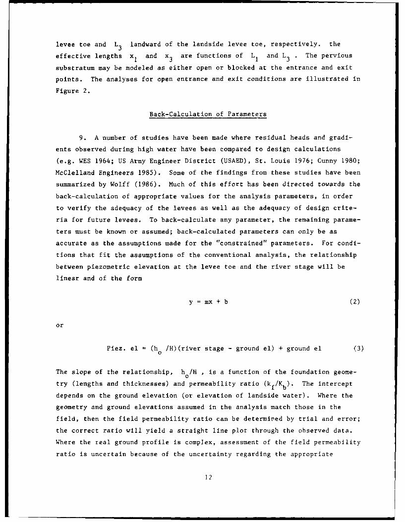
levee toe and L3 landward of the landside levee toe, respectively, the
effective lengths xI and x3 are functions of L and L3 ' The pervious
substratum may be modeled as either open or blocked at the entrance and exit
points. The analyses for open entrance and exit conditions are illustrated in
Figure 2.
Back-Calculation of Parameters
9. A number of studies have been made where residual heads and gradi-
ents observed during high water have been compared to design calculations
(e.g. WES 1964; US Army Engineer District (USAED), St. Louis 1976; Cunny 1980;
McClelland Engineers 1985). Some of the findings from these studies have been
summarized by Wolff (1986). Much of this effort has been directed towards the
back-calculation of appropriate values for the analysis parameters, in order
to verify the adequacy of the levees as well as the adequacy of design crite-
ria for future levees. To back-calculate any parameter, the remaining parame-
ters must be known or assumed; back-calculated parameters can only be as
accurate as the assumptions made for the "constrained" parameters. For condi-
tions that fit the assumptions of the conventional analysis, the relationship
between piezometric elevation at the levee toe and the river stage will be
linear and of the form
y = mx + b (2)
or
Piez. el = (h /H)(river stage - ground el) + ground el (3)o
The slope of the relationship, h /H , is a function of the foundation geome-0
try (lengths and thicknesses) and permeability ratio (k f/K b). The intercept
depends on the ground elevation (or elevation of landside water). Where the
geometry and ground elevations assumed in the analysis match those in the
field, then the field permeability ratio can be determined by trial and error;
the correct ratio will yield a straight line plot through the observed data.
Where the real ground profile is complex, assessment of tile field permeability
ratio is uncertain because of the uncertainty regarding the appropriate
12
Riverside Landside
kb
h =H h =0Lj,L2,L3 are actual distancesOpen 123open
entrance top blanket semipervious exit
x1 x2 3 -
k f
h =H h =0
x1 x2 ,x 3 are effective
x1 tanh (cL) x=L distances for impervious2 2 tcp blanket
kbr X3 =t nh(cL3
kf zd c
kblc = kz d
ifL = o x c 13 3 c
d
k b
Figure 2. TM 3-424 solutions for finite foundation lengths
13
"effective values" of the layer thicknesses and ground elevations. Different
permeability ratios will be back-calculated for different (although reason-
able) assumptions of effective layer thicknesses and elevations.
10. By using the programs developed herein, the foundation geometry is
more completely described, and fewer assumptions are required to make the
problem tractable. Thus, back-calculated permeability ratios should be more
reliable and less uncertain than those obtained from conventional analysis.
14
PART II: SPECIAL CASES OF FOUNDATION CONDITIONS
11. As previously stated, the conventional assumptions of 2-D flow and
a foundation profile of two uniform horizontal layers are not always consis-
tent with actual foundation conditions. For this research, three alternate
sets of assumptions have been identified and a computer program for the finite
difference solution of steady state laminar flow in porous incompressible
saturated media was developed for each. These special cases are representa-
tive of many prototype locations. In many cases, the relevant deficiencies of
the conventional method can be circumvented by selecting an appropriate
alternative. These alternate of "special" conditions are described in detail
below.
Foundations Characterized by Three Layers
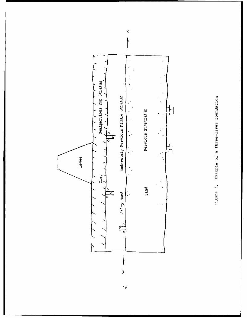
12. The special condition considered is the case of a foundation con-
sisting of three materials deposited in horizontal layers. The pervious mate-
rials immediately below a clay top blanket are often fine sand or silty sand,
while those at greater depth are typically medium or coarse clean sand. Such
layering is consistent with the geologic environment of a meandering stream,
where the expected grain size distribution is fining upward. In the developed
analysis, each of three layers may have different thicknesses and different
horizontal and vertical permeabilities. The layers are herein referred to as
the semipervious top blankct, moderately pervious middle stratum, and pervious
substratum. In such deposits, the top blanket may be a backswamp deposit, the
middle stratum may be a point-bar deposit of relatively uniform fine sands or
silts, and the pervious substratum is representative of a lower section in the
point bar or a "channel lag" deposit. Figure 3 illustrates a three-layer
foundation. Use of the conventional analysis requires that the analyst either
convert the middle stratum to a relatively thin equivalent layer of top blan-
ket, or consider it part of the substratum and average its relatively low
permeability with higher permeability values farther down the profile.
leither of these approaches may adequately model flow conditions along the
base of the top blanket. If the horizontal permeability of the middle stratum
exceeds the vertical permeability of the substratum, residual heads at the
15
Cd 0
cau
00
r--4
0 a
>b,(d,
00
N,,
16
base of the top blanket may be quite dependent on the properties of the middle
stratum, and less dependent on properties of the substratum.
Foundations Characterized by Two Layers of Irregular Shape
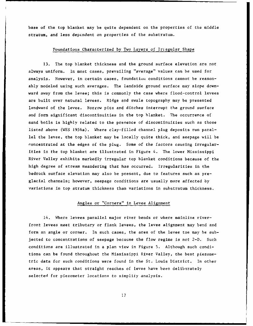
13. The top blanket thickness and the ground surface elevation are not
always uniform. In most cases, prevailing "average" values can be used for
analysis. However, in certain cases, foundatioit conditions cannot be reason-
ably modeled using such averages. The landside ground surface may slope down-
ward away from the levee; this is commonly the case where flood-control levees
are built over natural levees. Ridge and swale topography may be presented
landward of the levee. Borrow pits and ditches interrupt the ground surface
and form significant discontinuities in the top blanket. The occurrence of
sand boils is highly related to the presence of discontinuities such as those
listed above (WES 1956a). Where clay-filled channel plug deposits run paral-
lel the levee, the top blanket may be locally quite thick, and seepage will be
concentrated at the edges of the plug. Some of the factors causing irregular-
ities in the top blanket are illustrated in Figure 4. The lower Mississippi
River Valley exhibits markedly irregular top blanket conditions because of the
high degree of stream meandering that has occurred. Irregularities in the
bedrock surface elevation may also be present, due to features such as pre-
glacial channels; however, seepage conditions are usually more affected by
variations in top stratum thickness than variations in substratum thickness.
Angles or "Corners" in Levee Alignment
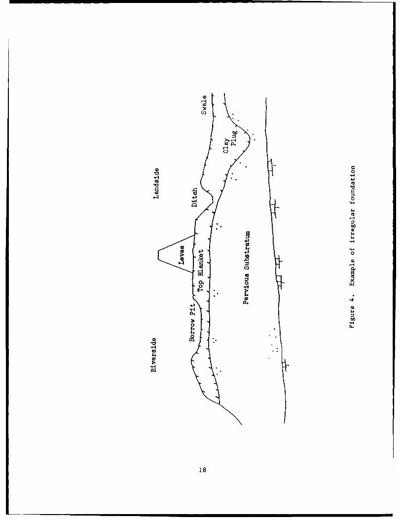
14. Where levees parallel major river bends or where mainline river-
front levees meet tributary or flank levees, the levee alignment may bend and
form an angle or corner. In such cases, the area of the levee toe may be sub-
jected to concentrations of seepage because the flow regime is not 2-D. Such
conditions are illustrated in a plan view in Figure 5. Although such condi-
tions can be found throughout the Mississippi River Valley, the best piezome-
tric data for such conditions were found in the St. Louis District. In other
areas, it appears that straight reaches of levee have been deliberately
selected for piezometer locations to simplify analysis.
17
00
.v-4q
0
41
4
* 4-) 4.4 0
000w
E-4-
CL14
0
-'-44
18
River
~Levee
Corner Landside
Seepage/toncentration in this area
Figure 5. Example of angle in levee alignment
19
PART III: SELECTION OF LEVEE REACHES FOR STUDY
Selection Criteria
15. Levee reaches in the Rock Island, St. Louis, Memphis, and Vicksburg
Districts were screened to identify reaches where actual performance could be
compared to predicted performance using the three developed computer programs.
Two criteria were considered: first, the reach must fit the particular
foundation conditions of interest (three layer, irregular, or corner) and
second, sufficient and reliable performance data must be available. The most
well-documented performance data are for those levee reaches reported by Cunny
(1980) for the Rock Island District, those reported by the St. Louis District
(USAED, St. Louis 1976), those reported by WES (WES 1956a and b, 1964) for the
Memphis and Vicksburg Districts, and those reported by McClelland Engineers,
Inc. (1985) for the Vicksburg District. Even from these sources, significant
amounts of data are missing or have been identified by the original analyst as
having questionable reliability.
Selected Reaches
16. The following reaches were identified in the preliminary screening
as fitting the conditions of interest and having reasonably accurate and
complete data. Those identified by an asterisk have been analyzed for this
report and are discussed in detail in Parts IV through VI. Locations of the
reaches analyzed are shown in Figure 6.
Foundations Characterized by Three Layers
* Rock Island District, Sny Island "F"
Memphis District, Caruthersville
Memphis District, Commerce
Vicksburg District, Upper Francis
* Vicksburg District, Eutaw
Foundations Charactcrized by Two Layers of Irregular Shape
Rock Island District, Sny Island, Range "G"
* Rock Island District, Hunt, Range "B"
Rock Island District, South Quincy, Range "SQ"
Rock Island District, South River, Range "SRC"
20

, Hunt
i - - / -II I
Sny Island
= Degognia
I I'R -
East Cape
SI .-"
Comme'rc - ./-1%, I Stovall S.
- .. I Bolivar, Eutaw
* . . 1 /
a I_ _ -- - , - -4\
Figure 6. Locations of analyzed levee reaches
21
Foundations Characterized by Two Layers of Irregular Shape (Continued)
St. Louis District, Perry County, Sta 329+85
Memphis District, Gammon
* Memphis District, Commerce
* Memphis District, Stovall
* Vicksburg District, Bolivar, Range "D"
Angles or "Corners" in Levee Alignment
Rock Island District, Bay Island, Range C
St. Louis District, Columbia Sta. 653
* St. Louis District, Degognia Sta. 260-290
St. Louis District, Grand Tower Sta. 430
* St. Louis District, East Cape Sta. 94
St. Louis District, East Cape Sta. 309
Memphis District, Farrell
Memphis District, Stovall
Vicksburg District, Bolivar, Range "D"
22
PART IV: FOUNDATIONS CHARACTERIZED BY THREE LAYERS
Numerical Modeling Technique
17. To analyze underseepage conditions for foundations consisting of
three layers, a computer program named LEVEE3L was written. Given the thick-
nesses and effective lengths of the layers, LEVEE3L generates a grid of
96 points or nodes (8 rows by 12 columns) and solves the differential equation
for 2-D flow at each node using the finite difference method. The spacing
between the nodes varies in both the x- and y-directions and is a function
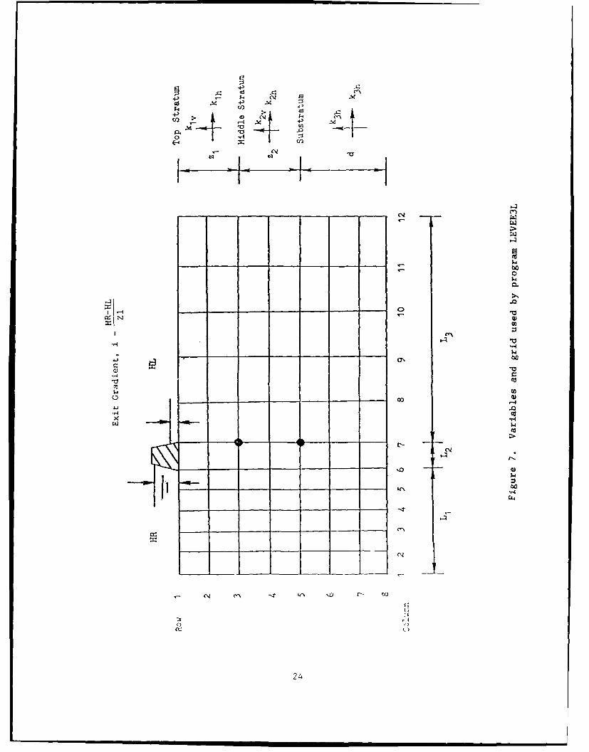
of the specified geometry. Figure 7 defines the variables used by LEVEE3L to
describe the problem geometry and illustrates the generated grid. The ground
surface coincides with Row 1, the base of the top blanket coincides with
Row 3, the base of the middle stratum coincides with Row 5, and the base of
the substratum coincides with Row 8. Column 1 corresponds to an open
entrance, and Column 12 corresponds to an open exit. Infinite L or L3
distances are modeled by specifying very large values, as is traditionally
done in finite element modeling. The landside levee toe is at Column 7. The
exit gradient is obtained by dividing the excess head at node (3,7) by the
thickness of the top blanket. The finite difference equation for flow at an
interior node is shown in Figure 8. Use of the program LEVEE3L is described
in Appendix A. Results of the program are compared to the other programs in
Appendix D.
Effect of Moderately Pervious Middle Stratum
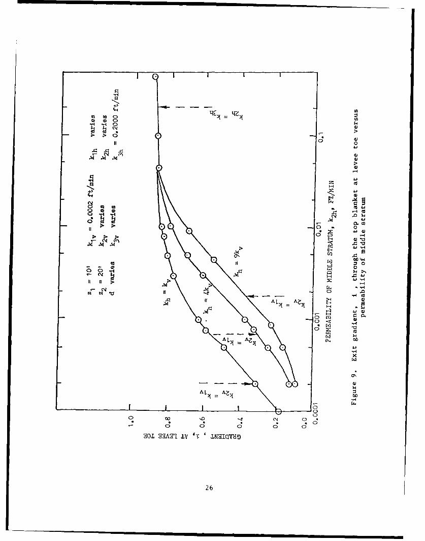
18. The effect of a middle stratum was initially investigated by using
the program to perform a series of parametric studies. Results of these
studies are illustrated in Figures 9 through 11. For all parametric studies,
the base width of the levee was arbitrarily taken as 50 ft and the differen-
tial head was taken as 20 ft. Most real levees of 20-ft height would have a
wider base width; this would tend to reduce the calculated gradients somewhat.
In the first study, constant foundation geometry was assumed, and the ratio of
the vertical permeability in the top blanket (k lv) to the horizontal permea-
bility in the substratum (k3h) was assumed to be 1,000. Then the exit gradi-
ent through the top blanket, i , was evaluated et point 1, 7 in Figure 7
23
4'
4) .- 5-4 N ~ -~
aS .~ ~'(0 4'
-p(J2 ONI I-i~ -Pul
(12
N *0
I_______________________
- -- - N1~
$4
0$4
.0
'-4 - - - - - - - 01*~ 0)
02
.4
_____ $4-I-- - - e~o
0"-4
$4 02
__ 0J02.0CU
$4CU
C-N
.4 I.-
-- '0 0)$4
ft - - __ - - _ U-'$4..
N
~- N (~\ ~ .4-' '0 t~ CO
:1-4
0 0
a: (9
24
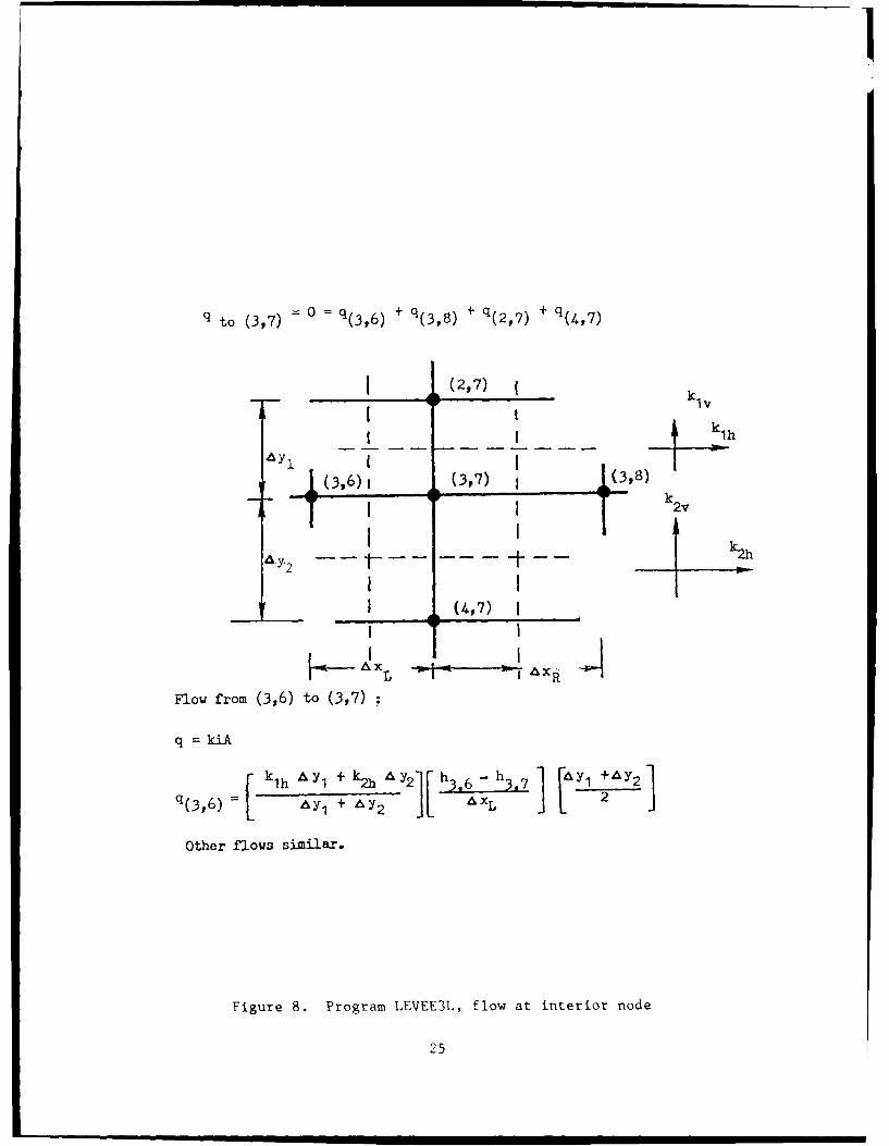
q to (3,7) 0 = q( 3 , 6 ) + q( 3 , 8 ) q( 2 , 7 ) + q(4,7)
S(2,7) k
_ _ k~
kvI I1 I
I I
I4
Flow from (3,6) to (3,7) :
q= kiA
f klh A~ + kh Y2 1[ h3 ,6 - h37] [ Y +Ay2 1
q(,) y I +i my 2 -L AXL 2 ]
Other flows similar.
Figure 8. Program LEVEE3L, flow at interior node
25
• . i a l l I& 2 2-h iIq
M qLZ U)*.-4 0
> >
II o
cm m 0
C; -4
-p0 0)
004 >
tl 0 It 0
0m
700
$4
If 0
-0-AVL. - 0
1 0.-C;
0 0 0 0
201 a~ar Ltv mal)
26-
(4-4
C3 m 0*i 00
-0
:1 >0_T5 Al
-0E-4 -
4~44
00 >00 LJW
> > >0-
P.4 $4.
U) >
4))
0 0
301V 00A IV' IN
'0 C27

.4-3
4)o 000 0
> 0
r+4 4-4-.
c'0 tt 0
o 4*4
*
4 -'4
~0*rU,
IN,
CIN E- 9
Cf)
-4
510 99H I'L-1(vl
28
as a function of the permeability of the middle stratum and the permeability
ratio within each stratum. The results are presented in Figure 9. It is
shown that the gradient increases as permeability of the middle stratum
increases and the gradient decreases as the permeability ratio within the
layers increases.
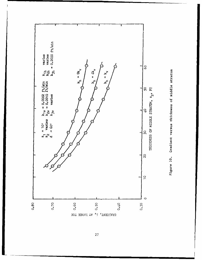
19. In the second study, the thickness of the top blanket, thickness of
the substratum, and the vertical permeabilities were fixed and the gradient
investigated as a function of middle stratum thickness and permeability ratio.
The results are presented in Figure 10. It is shown that the gradient
decreases as the middle stratum thickness increases and the gradient increases
as the permeability ratio within the layers increases.
20. The third parametric study was similar to the second except that
the thickness of the middle stratum was fixed and the thickness of the top
blanket was varied. The results are shown in Figure 11. It is shown that the
gradient decreases as the top blanket thickness increases (as is well known)
and that the gradient decreases as permeability ratio increases.
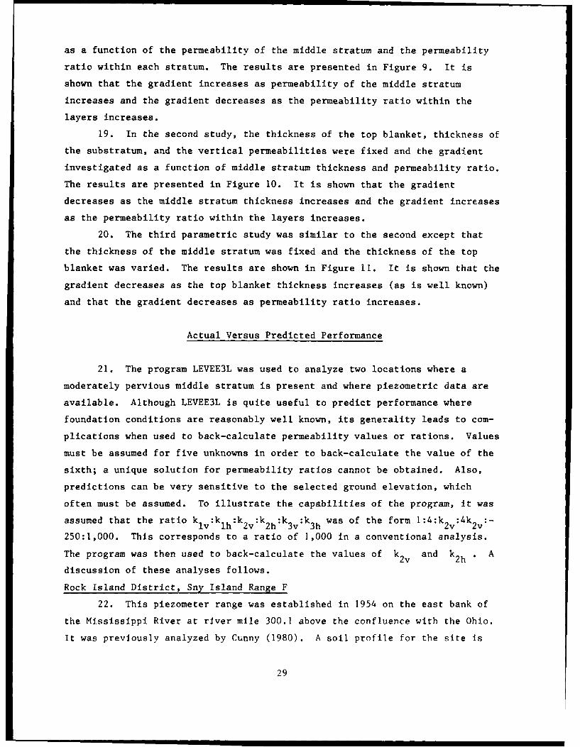
Actual Versus Predicted Performance
21. The program LEVEE3L was used to analyze two locations where a
moderately pervious middle stratum is present and where piezometric data are
available. Although LEVEE3L is quite useful to predict performance where
foundation conditions are reasonably well known, its generality leads to com-
plications when used to back-calculate permeability values or rations. Values
must be assumed for five unknowns in order to back-calculate the value of the
sixth; a unique solution for permeability ratios cannot be obtained. Also,
predictions can be very sensitive to the selected ground elevation, which
often must be assumed. To illustrate the capabilities of the program, it was
assumed that the ratio k lv:k lh:k 2v:k2h:k3v:k3h was of the form :4:k 2v:4k2v:-
250:1,000. This corresponds to a ratio of 1,000 in a conventional analysis.
The program was then used to back-calculate the values of k2v and k2h . A
discussion of these analyses follows.
Rock Island District, Sny Island Range F
22. This piezometer range was established in 1954 on the east bank of
the Mississippi River at river mile 300.1 above the confluence with the Ohio.
It was previously analyzed by Cunny (1980). A soil profile for the site is
29
shown in Figure 12. The top stratum thickness ranges from 4.8 to 10.0 ft and
generally consists of 2 to 4 ft of lean clay overlying silt and silty sand.
Considerable seepage has been reported at this location: toe seepage, sand
boils and pin boils in 1960, pin boils in 1965, and light toe seepage in 1973.
These observations do not correlate well with river stage, as stages were the
highest in 1973 and lowest in 1960. These discrepancies may in part be
related to levee enlargement between 1965 and 1967 and provision of a berm
that lengthened the effective base width.
23. Parameters used in the analyses are listed in Table 1. The column
labeled "conventional analysis" summarizes values presented by Cunny (1980).
Using LEVEE3L, the profile was modeled as a 3.0-ft-thick clay top blanket
overlying a 5.0-ft-thick middle stratum. Two computer analyses are reported.
In analysis "A," the landside distance to an open exit, L3 , was taken as
3,000 ft to represent a foundation with infinite landward extent. Analysis
"B" was made assuming L3 as 400 ft to match the observed sluggish response
of piezometer F-4, which suggested that most of the seepage was exiting
relatively close to the levee. Results of the computer analyses are plotted
with the actual data in Figures 13 through 16. A reasonable match to the
observed performance was obtained using a permeability ratio of 1:4:50:200:-
250:1,000. Although the finite difference grid was developed primarily with
the purpose of assessing heads and gradients at the levee toe, heads and
gradients for other piezometer locations were determined by interpolation of
the final heads reported in the program output file. The results of analyses
"A" and "B" are virtually identical in the vicinity of the levee, but analysis
"B" provides a better match remote from the levee.
24. A shortcoming shared by b. -- the conventional analysis and the
three-layer analysis is the need to assign a single value for the ground ele-
vation when the ground is in fact uneven. The appropriate ground elevation
for analysis can be inferred from piezometric response using Equation 3 in
this report, as the residual head should be zero for a river stage equal to the
landside ground elevation. A value of 457.5 was determined by extrapolating a
line through the piezometric data down to a point where the piezometric eleva-
tion matched the river elevation. This ground elevation is 2.0 ft lower than
the ground elevation at piezometer F-3 assumed by Cunny (1980) with the result
that higher residual heads are predicted herein. For a river stage of 472.8
(levee crest), the predicted piezometric elevation at F-3 is 460.8. This
30
0c1~ W
z 0
00
00
o o
o a
ol
311

Table 1
Parameters Used for Analyses, Rock Island District,
Syn Island, Range F
Conventional LEVEE3L LEVEE3LAnalysis Analysis Computer ComputerParameter* (Cunny 1980) Analysis "A" Analysis "B"
L (ft) -- 510 510
L2 (ft) -- 100 100
L3 (ft) Infinite 3,000 400
zI (ft) 6.9 ft at F-3 3.0 3.0
z2 (ft) -- 5.0 5.0
d (ft) 34 34.0 34.0
k V (ft/min) -- 0.0002 0.0002
klh -- 0.0008 0.0008
k2v 0.0100 0.0100
k2-- 0.0400 0.0400
k3v -- 0.0500 0.0500
k3h -- 0.2000 0.2000
kf/kl 31 1,000 1,000
Levee crest 472.8 472.8 472.8
Ground el 459.5 457.5 457.5
s (ft) 219 -- --
x3 (ft) 108 ....
h at Rm 1.3 at F-3 5.0 at F-3 3.3 at F-3o max
* Defined in Figures 2 and 7.
32

C-)
04.j
0
N
co)0
-4o
'C:0
00
-4-40).
U-\~ 0 a
N' #4 - E-
a' '-1-4 r 0 4-
t-E-4
93 >4.'03
'0- -)&
>o u0 0
Hw
Q 0-E3010 0,
A4 3 u 4-0
0 ~ 0
-4--1
01:Uco-
GAORLi 'OLLVTM DU131IMa,
I 33
CIDIto W
0
ik\ N
-r4
la
- 00
-4 -4 4.
a E-44
'0 - -- 0 -4
0 R a)
4 00 4P -) aC-3 'U r4
00
co -4
N 434
000
000
CVN
%0 cc
C,\ 1--40A
003
til > t-'4-
C;O
1-4 -4(D t 0s.De~'
4- -4 ;4
V-400 r4
0q 0 Q
$4 Cd
0 I,-'
000 cc
C--
C.A00 Li'OCOMOJ~W~
35i
CwLA
rz
coL--4 cn Zt
0
0 ___ __ __ __ __
0't'i 0 0 eA'
0 >
(IMY'4~~- 'Ji'"LV 4:
corresponds to a head of 3.3 ft. As the tip of F-3 is located below the base
of the middle stratum, the exit gradient at F-3 depends on the assumption made
for the effective top blanket thickness.
25. As F-3 is some distance landward of the levee toe and below the
middle stratum, it does not directly provide information regarding seepage
conditions in the top blanket at the levee toe. The computer solution gives a
residual head of 5.60 ft at this point with the river stage at the levee
crest. Dividing this value by a top blanket thickness of 3.0 ft, a gradient
of 1.87 is obtained, well above critical. This is consistent with past
observations of heavy seepage and boiling at Sny Island and indicated that the
boils are likely related to the presence of relatively thin clay top blanket
deposits underlain by silty middle strata that provide little seepage
resistance.
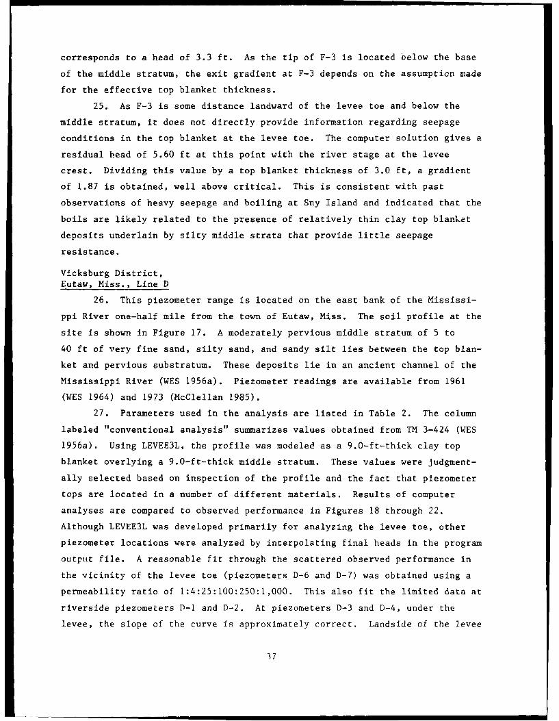
Vicksburg District,Eutaw, Miss., Line D
26. This piezometer range is located on the east bank of the Mississi-
ppi River one-half mile from the town of Eutaw, Miss. The soil profile at the
site is shown in Figure 17. A moderately pervious middle stratum of 5 to
40 ft of very fine sand, silty sand, and sandy silt lies between the top blan-
ket and pervious substratum. These deposits lie in an ancient channel of the
Mississippi River (WES 1956a). Piezometer readings are available from 1961
(WES 1964) and 1973 (McClellan 1985).
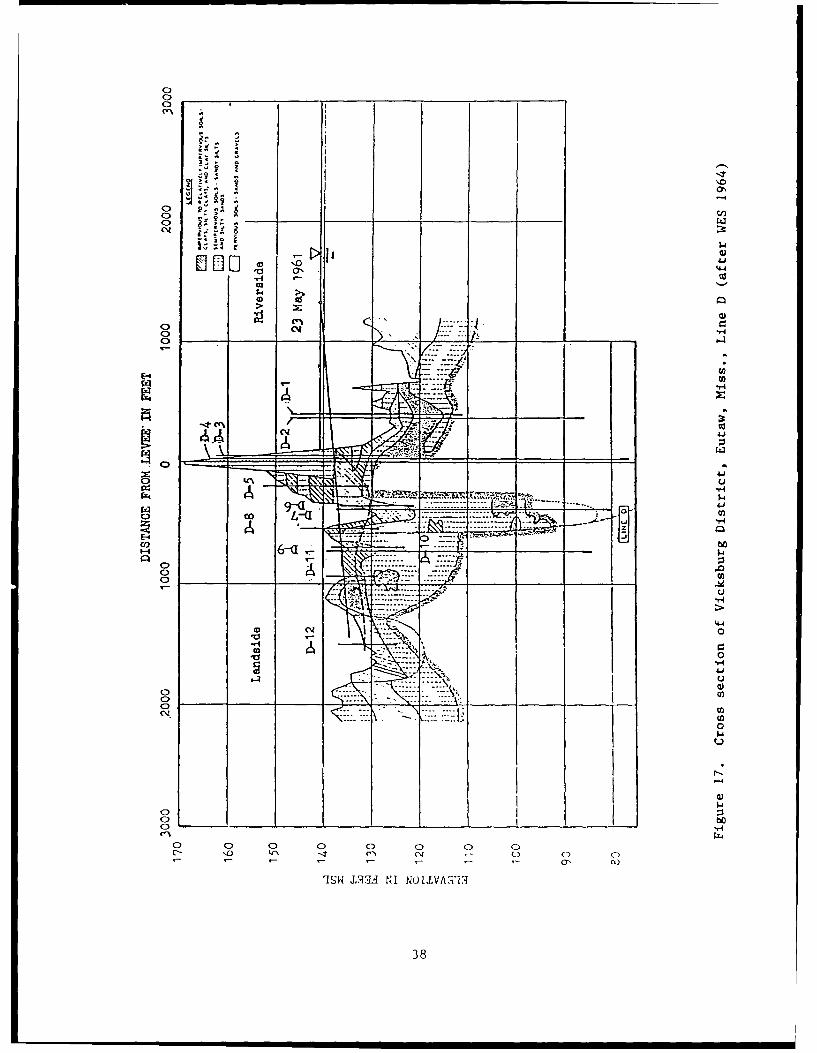
27. Parameters used in the analysis are listed in Table 2. The column
labeled "conventional analysis" summarizes values obtained from TM 3-424 (WES
1956a). Using LEVEE3L, the profile was modeled as a 9.0-ft-thick clay top
blanket overlying a 9.0-ft-thick middle stratum. These values were Judgment-
ally selected based on inspection of the profile and the fact that piezometer
tops are located in a number of different materials. Results of computer
analyses are compared to observed performance in Figures 18 through 22.
Although LEVEE3L was developed primarily for analyzing the levee toe, other
piezometer locations were analyzed by interpolating final heads in the program
output file. A reasonable fit through the scattered observed performance in
the vicinity of the levee toe (piezometers D-6 and D-7) was obtained using a
permeability ratio of 1:4:25:100:250:1,000. This also fit the limited data at
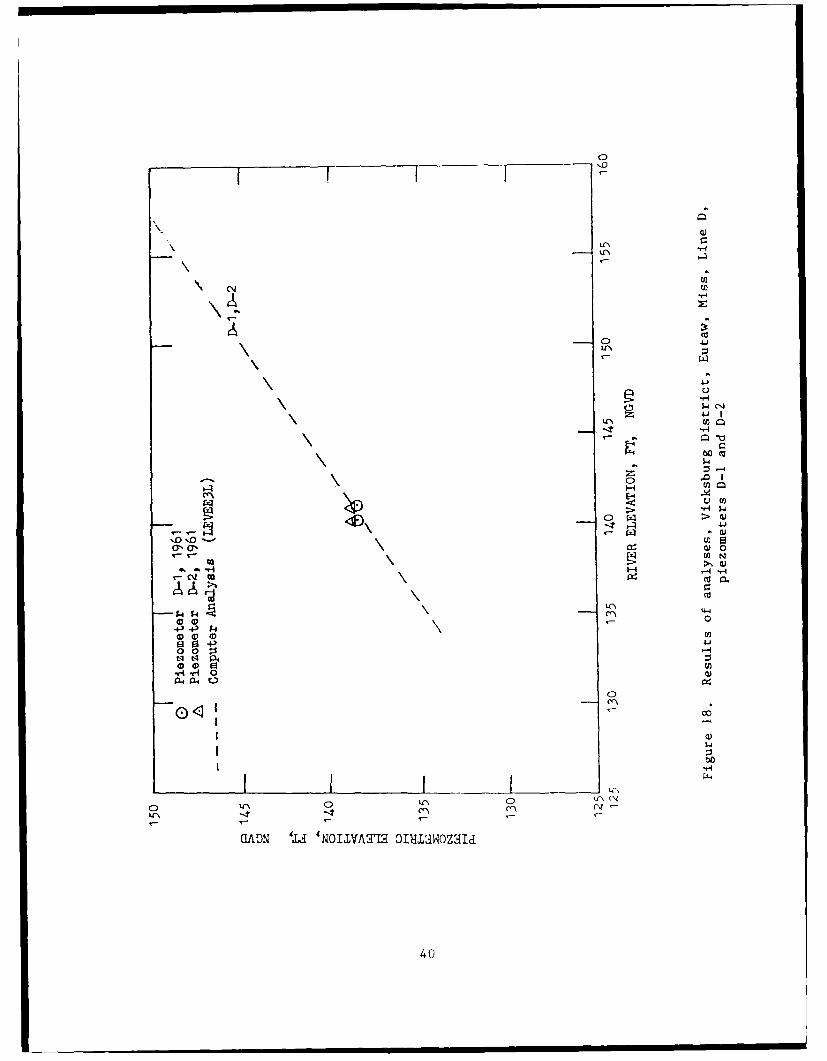
riverside piezometers P-I and D-2. At piezometers D-3 and D-4, under the
levee, the slope of the curve is approximately correct. Landside of the levee
37
104 44
0 Of0
E--4
ot0~~ _ __ _ _
o-- Hz4
302
C))
ob
oo
.4- W IRM N1N IJA-'
38L

Table 2
Parameters Used for Analyses, Vicksburg District,
Eutaw, Miss, Line D
LEVEE3L
Analysis Conventional Computer
Parameter* Analysis Analysis
LI (ft) 2,500 2,500
L2 (ft) -- 450
L 3 (ft) Infinite 750
z (ft) 18.0 9.0
z2 (ft) -- 9.0
d (ft) 70.0 70.0
k (ft/min) -- 0.00022
klh 0.00088
k2v -0.0055
k2h 0.0220
k3v -- 0.0550
k3h 0.2200 0.2200
kf/kbl 800 --
Levee crest 161.0 161.0
Ground el 135.0 135.0
s (ft) 1,500 --
x3 (ft) 1,000 --
h at H 10.4 8.00 max
* Defined in Figures 2 and 7.
39
0
~rn
o 4-o
zz
u
-t~
0 Al
u I
0 w0 Q
(7,a, Q)
000
0 0 ::%t-I N 4 20 0 93U
0
-40
10
V,-
0I
A J-J
u
-4-J
E-4 CO4
u w
U S. w 0 O
-P -
0 0 0 0
0D E3
ClCO
LI 0
IA UN JA4 'NOI.LVATI:I, 3PILJWN07,:Ild
41
0*L9L '4W GaAaGj C
>'0
El w
T -1It0 ud
Ca >
>~
aa% >a
a'aUa 0W\% C- c0
00CD0 0+4-31 -P 3 4 4-'3 0 000 4' 0
13 43 V.0 00 :1 (atq N~ eq P4 400 =Z-
-H ,, 4 0 0PL4 P OC)
00LI 0 c'4
QIAON 'M± 'NOILVAaIS H{OLVATIa 0OLIUOZaId
42
* tca
AA
'U
JJ0C.0 p
02.
kC P.P 4.t -r I
4- 4-'.0 '-1'0 (D.0 0 4-40 0"0 :
4) (D 02 M' j
P~4 P4 0 4
00
N U- CV %2, 00 0 -4.
434
U-0'
0 ID
"- NJ
ooo
0 o :5 4
A' 04 (00
GA O 4 J4 i OLLVSU O"HIHMII
44 ,-
toe, the predictions fall on both sides of observed data, depending on the
piezometer location analyzed.
28. The great variability in piezometric response at this site points
up the problems inherent in analyzing irregular soil profiles. Despite the
ability of LEVEE3L to account for the thick silt layer below the clay tup
blanket, the analysis remains uncertain and subjective because the irregular
grond ,rface elevation P top blanket thickness must be treated as single
"effective" values. It appears that the program LEVEEIRR described in Part V
of this report offers some advantage over LEVEE3L for such conditions, and it
may be desirable to develop a program that combines some of the features of
both.
45

PART V: FOUNDATIONS CHARACTERIZED BY TWO LAYERS OF
IRREGULAR SHAPE
Numerical Modeling Technique
29. To analyze underseepage conditions for foundations consisting of
two layers of nonuniform thickness with non-horizontal boundaries, a computer
program named LEVEEIRR was written. LEVEEIRR solves the same differential
equation for the same assumptions as Bennett's (1946) solution; however, the
soil boundary elevations and the layer thicknesses a and d need not be
constant but may vary as a piecewise linear function of horizontal distance
x . Input to the program coiisists of the same parameters used for
conventional analysis, with the addition that the elevations of the top of the
blanket, top of the substratum, and bottom of the substratum are specified for
a selected set of x-coordinates. Between each specified x-coordinate, the
program generates nine additional nodes along the interface between the top
blanket and substratum. The head at each node is calculated by iteratively
solving a finite difference equation for the flow at each node. The technique
used in LEVEEIRR is illustrated in Figure 23. The program output provides the
residual head and gradient at every node point, and thus allows calculation of
the expected gradient at local discontinuities such as landside ditches, thin
spots in the top blanket, and edges of clay plugs. The use of LEVEEIRR is
described with examples in Appendix B.
Effect of Nonuniform Layer Thickness
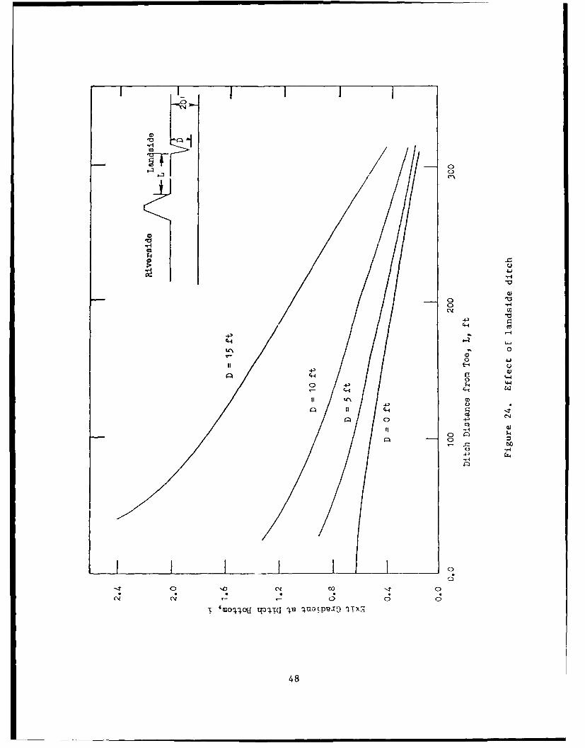
30. To illustrate the capabilities of LEVEEIRR, the common problem of
excavating a ditch adjacent to a levee was investigated. It was assumed that
the top blanket had a uniform thickness of 20 ft before excavating the ditch.
If was further assumed that the thickness of the substratum was 100 ft, the
net head on the levee was 20 ft, and the permeability ratio was 500. The
depth of the ditch, D , and the distance from the ditch crown to the levee
toe, L , were then varied and the gradient at the bottom of the ditch plotted
as a function of the two variables. Results of the analysis are shown in
Figure 24. As would be expected, it is shown that the gradient increases with
increasing ditch depth and decreases with increasing distance from the levee.
46
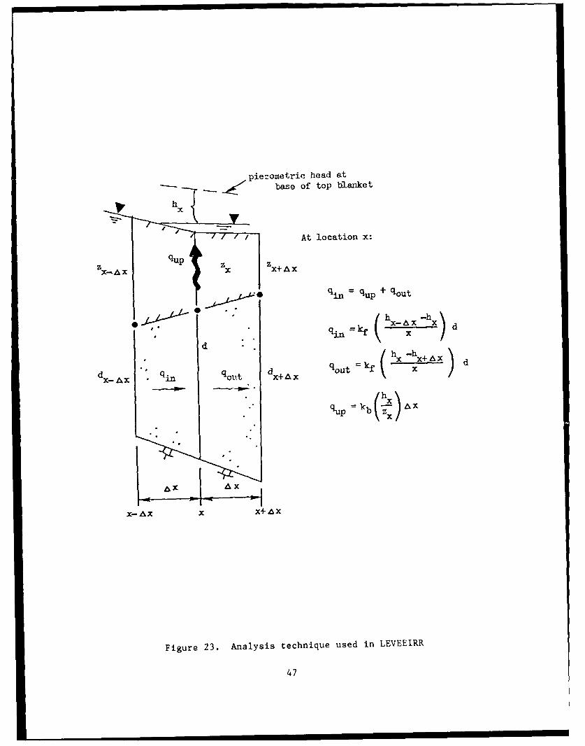
piezometric head at
base of top blanket
T At location x:
d
dx-. i ot d+x qut kf (xX -xAX
x
-p
z-C z x z
x-A x +Ax
Figure 23. Analysis technique used in LEVEEIRR
47
1 q I I - q + I I I II
.01
0
0.C~l U
4-1I
LC\ 0
0 4
4-4
-4-4-4
4-4 U-.
0 C>
48'
DISTANCE- FEET FROM CENTER LINE OF LEVEE500 400 300 200 100 0 100 200 300 400 500
510
500 _.. .... -d ......
0
0 i.H470
STATION t3g+25460
a. Ac ual ross ectiIn I Afterl Cunny 198 )450 - !- - - - -- - - - - -
1000 800 600 400 200 0I I I I I
I /Levee Riverside
490
480
0'-4
m 470
b. Modeled ross secti n338 -1 -- -u
Figure 25. Actual and modeled cross section of Rock Island
District, Hunt, Range "B"
50
Actual Versus Predicted Performance
31. The program LEVEEIRR was used to analyze four levee reaches having
markedly irregular subsurface conditions. For each reach, the assumed perme-
ability ratio was varied to find the ratio that best corresponded to observed
performance. A discussion of zhese analyses and results follows.
Rock Island District, Hunt, Range B
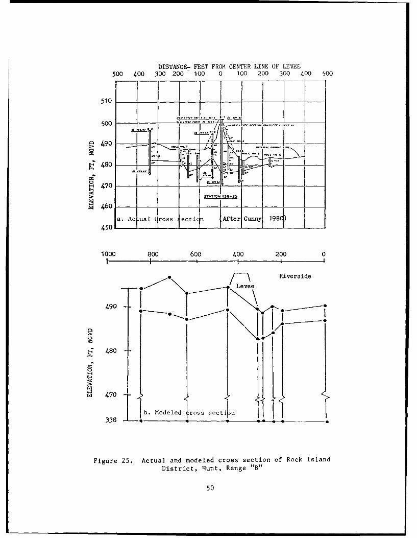
32. This piezometer range was establijned iii 1957 on the east bank of
the Mississippi River about 25 miles upstream from Quincy, Ill., in the pool
area of Lock and Dam 20. It was previously analyzed by Cunny (1980). A
foundation profile and the idealized section used for computer modeling are
ohown in Figure '5. Irregularities in the profile include a landside ground
elevation about 5 ft higher than the riverside and an impervious top stratum
varying from 5.3 to 8.2 ft thick. There are three piezometers at the site:
B-i near the levee crest, B-2 near the levee toe, and B-3 on a small ridge
about 350 ft landward of the levee centerline.
33. Parameters used in the analyses are shown in Table 3. Piezometric
elevations calculated using LEVEEIRR are compared to observed piezometric
elevations in Figure 26. Two computer analyses were performed. Analysis "A"
assumed a permeability ratio of 64, the same as the value used by Cunny.
Although this value provided a reasonable match to the observed data at the
tiree piezometer locations, a somewhat better fit was obtained by reducing the
top blanket permeability until the permeability ratio was 20. The latter
results are labeled analysis "B." It should be noted that LEVEEIRR is capable
of predicting piezon:etric elevations even where they are below ground level,
as is the case for B-i and B-3, so long as there are artesian (confined seep-
age) conditions in the pervious substratum. Assuming a flood level at the top
of the levee (501.5) and an interior water elevation of 487.0, a maximum
gradient of 0.73 is predicted to occur at the landside levee toe near
piezometer B-2.
Memphis District, Commerce, Miss., Line H
34. This piezometer range was established in 1942 about 10 miles north
of Tunica, Miss. Heavy seepage damage was reported at the site during the
1937 high water. The levee is located about 2,200 tt from the Mississippi
River on terrain characterized by numerous ridges, ditches, and swales. A
foundation profile and the Idealized crnss section used for analysis are shoun
49
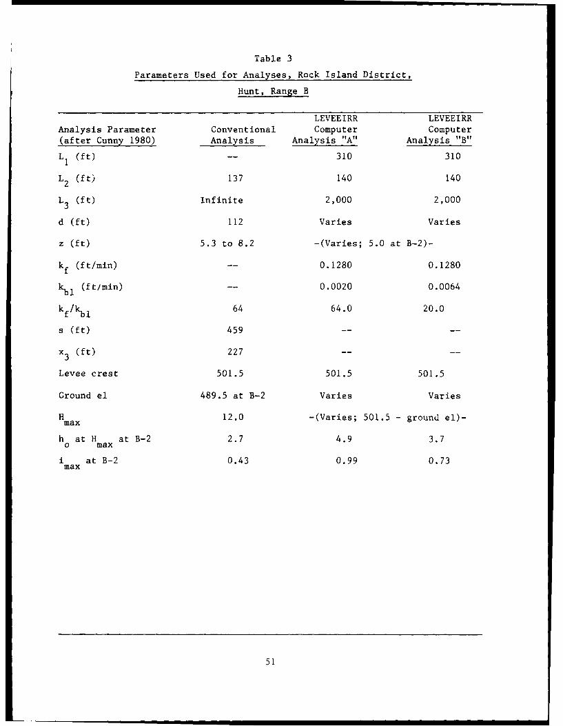
Table 3
Parameters Used for Analyses, Rock Island District,
Hunt, Range B
LEVEEIRR LEVEEIRR
Analysis Parameter Conventional Computer Computer(after Cunny 1980) Analysis Analysis "A" Analysis "B"
L 1 (ft) -- 310 310
L2 (ft) 137 140 140
L3 (ft) Infinite 2,000 2,000
d (ft) 112 Varies Varies
z (ft) 5.3 to 8.2 -(Varies; 5.0 at B-2)-
kf (ft/min) -- 0.1280 0.1280
k bi (ft/min) -- 0.0020 0.0064
kf /k bl 64 64.0 20.0
s (ft) 459 ....
x 3 (ft) 227 ....
Levee crest 501.5 501.5 501.5
Ground el 489.5 at B-2 Varies Varies
H 12.0 -(Varies; 501.5 - ground el)-max
h at H at B-2 2.7 4.9 3.7o max
i at B-2 0.43 0.99 0.73max
51

U,
-4 '-4
O
ON
-4 0
a%(NON C
-4-4 -4 a
ONNO
-4 -4 U,)-
4. 4 -1 u4 $4
03~K 0 0 : :
030) 0 a03
40 .14
A4 P4
(D <
It)
o ON
I)U
C)
'4-4 LW-
IL Cf) ~'
C, (D CYN 00O
5 2
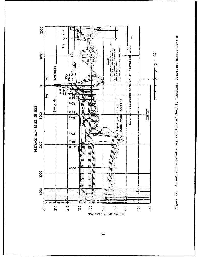
in Figure 27. Seventeen piezometers were used for analysis at this section.
Piezometric data were obtained in 1961 (WES 1964). As some of the piezometers
are located on different but adjacent levee cross sections, some variation is
observed for piezometers that are about the same distance from the levee.
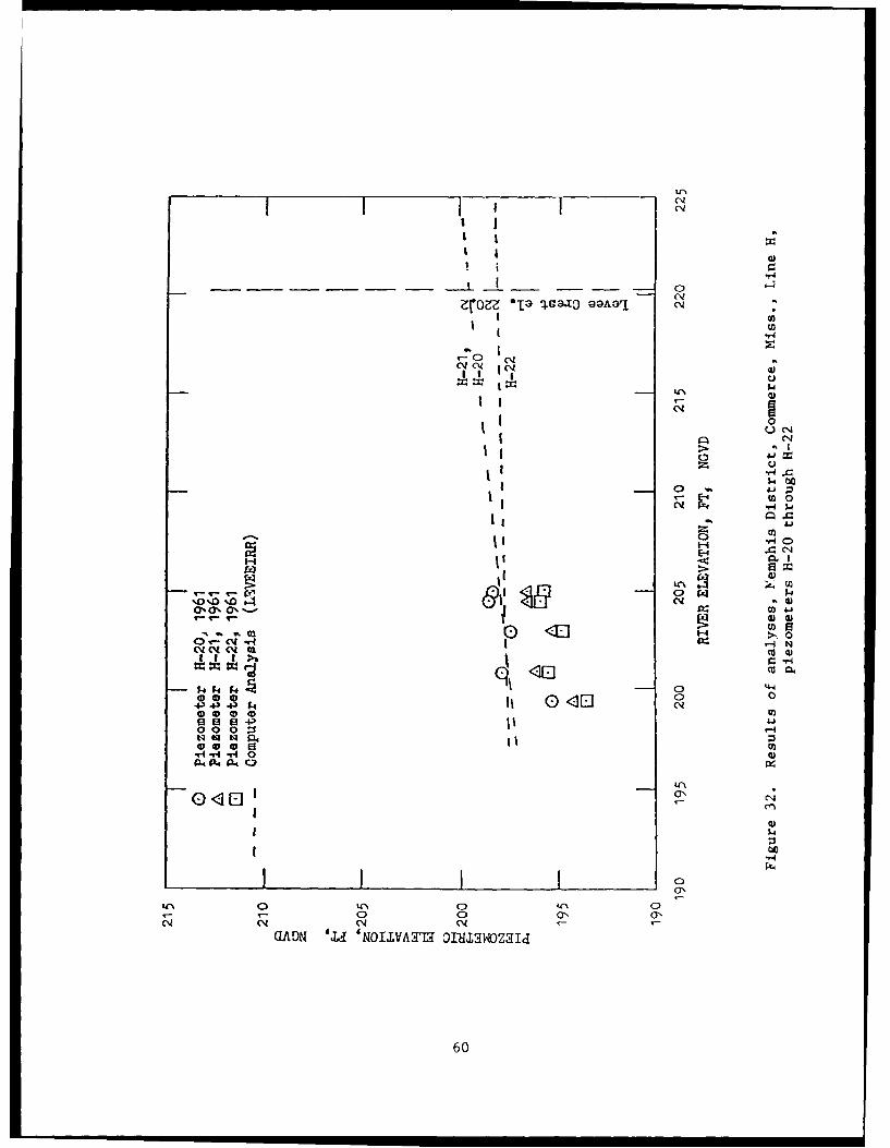
35. Parameters used for analysis are shown in Table 4. The column
titled "Conventional Analysis" provides values reported in TM 3-424 (WES
1956a) for comparison. Piezometric elevations calculated using LEVEEIRR are
compared to observed data in Figures 28 through 32. The predictions are based
on a permeability ratio of 514, a value that was calculated using the two
permeability values reported in TM 3-424. (Permeability ratios and permeabil-
ity values reported in TM 3-424 are not exactly consistent). It should be
noted that reasonable predictions can be obtained using LEVEEIRR for widely
different distances from the levee toe.
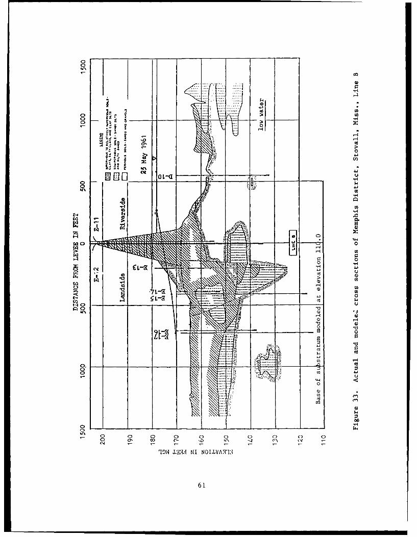
Memphis District,Stovall, Miss., Line B
36. This piezometer range was established in 1948 about 3.5 miles west
of Stovall, Miss. Seepage damage occurred at the site during the 1937 high
water. A foundation profile and the idealized cross section used for analysis
are shown in Figure 33. Irregularities in the profile include a very thin
riverside top stratum due to removal of borrow materials, a thick landside top
stratum, and a silt plug below the levee centerline. Piezometric data were
obtained in 1961 (WES 1964).
37. Parameters used for analysis are shown in Table 5. The column
titled "Conventional Analysis" provides values obtained from TM 3-424 for com-
parison. Two analyses using LEVEEIRR are reported. In analysis "A" the
permeability ratio was taken as 432, the ratio of the two individual values
reported in TM 3-424. For analysis "B" the permeability ratio was taken as
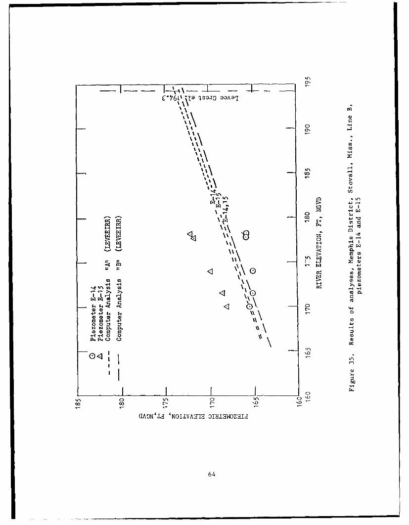
1,000. Piezometric elevations calculated using LEVEEIRR are compared to
observed data in Figures 34 through 36. it is noted that the computer solu-
tions plot below the observed data for piezometers in the substratum (E-15 and
E-17) by several feet. Relatively high piezometric response has been observed
at these piezometers. The profile at Stovall is an extreme case of different
blanket materials and thicknesses on opposite sides of the levee. It is
likely that the top blanket permeabilities are also much different on the two
sides. Attempts to match the response of E-15 and E-17 by decreasing the
riverside blanket thickness, increasing the permeability ratio, and shortening
53
C3AS %S
C))
00
4-44
I.
ww
0Ei -
ala
o0 _ _ 4-4U)U
41i
E0 0)
000 cc
00
ca
El,
'19W 0 OUA
1454
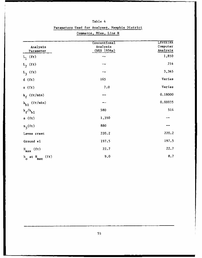
Table 4
Parameters Used for Analyses, Memphis District
Commerce, Miss, Line H
Conventional LEVEEIRR
Analysis Analysis Computer
Parameter (WES 1956a) Analysis
L1 (ft) 1,850
L2 (ft) 214
L3 (ft) -- 3,365
d (ft) 165 Varies
z (ft) 7.0 Varies
kf (ft/min) -- 0.18000
k ,1 (ft/min) -- 0.00035
kf/kbl 580 514
s (ft) 1,350 --
x3 (ft) 880 --
Levee crest 220.2 220.2
Ground el 197.5 197.5
H (ft) 22.7 22.7max
h at H (ft) 9.0 8.7o max
55
__ CV
-H
0
'u I
lipl
WI
U)0
CYN ON -
< C) C:
%D CC 0
(V
000
CU)
434
(D 0 56
cC\4
- - -- H
W
E-U,
9"-
Coo44 0
13
0 0 0
00
cvN
-4'r- 0 1W14l Of .l
QADNId '40IJAT~ DIH IM4ZOI
57~
0
C\1o
V14
(w~E-4 co4
a 4
.4v
C-1
a 00
(D 4-
a0 I 0 4.
00 v
P, ca
I 2.4
oa
''0 0C 0ca-00 O\ a5'
CLAN 'QZ 'NOLLVAT 0U-H-I9iL3OZq-Te
58
z -oz -l -S-T ;O 21 go
*14
- w)
1053
cvI
' I y-4t
0% 10
0
ID W-(4 a)4JA
ci a
00 n
0000Of4 04 ol 0
(ID til 'KL'4.'H~W~ac
594
ZIo -l SaNa~r
CN
u Cl)
(A 0~-o N
-r C
CNON
ON a, ONh4) W
C)LC'o'o' N C4 m m 4)j
a. r. -H
Nk F4 4-
0 0 0 Ii In NI0N
ON0 C14
d 04. 00~1400 0~C
0<60
00
441
--. 0
'0ol
k-40'
00
0 C)
CD __ coL H- '-CVo
'10W IM NI NLLV-4
61o
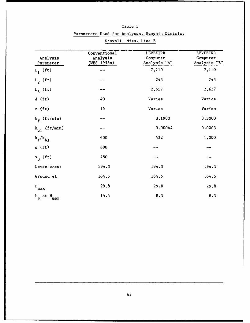
Table 5
Parameters Used for Analyses, Memphis District
Stovall, Miss. Line B
Conventional LEVEEIRR LEVEEIRRAnalysis Analysis Computer ComputerParameter (WES 1956a) Analysis "A" Analysis "B"
L (ft) -- 7,110 7,110
L2 (ft) -- 243 243
L3 (ft) -- 2,657 2,657
d (ft) 40 Varies Varies
z (ft) 15 Varies Varies
kf (ft/min) -- 0.1900 0.3000
kbl (ft/min) -- 0.00044 0.0003
kf/kbl 600 432 1,000
s (ft) 800 -- --
x3 (ft) 750 -- --
Levee crest 194.3 194.3 194.3
Ground el 164.5 164.5 164.5
H 29.8 29.8 29.8max
h at H 14.4 8.3 8.30 max
62

0'0
imca
00 \ 0
-4 cQ D\ 4j
W0
Lrr04
IkA .4 14W02 0
0 00
0 0 z 3-t4 t4 0. P. XX'
-H- 0 0 0)4PW 914 Q) ca
o toi
GADtM 6l NOILVAMT OnAla1OZaI
63
C*760 a is-o a 0Aa
00
-&C\
Z4 WI
irz
0)
0
0 1~- 4-4
0 0 :
. f4 ) C0)
LCA 0'
(I ON.- la'O V M DIINP ~
oo~ :~ .64
co
Ct ID
CO -
4)0
I* N
E-44
0 m 0 : 0
03 00
00 coc-C
.d.w 00IVTaODaq~~
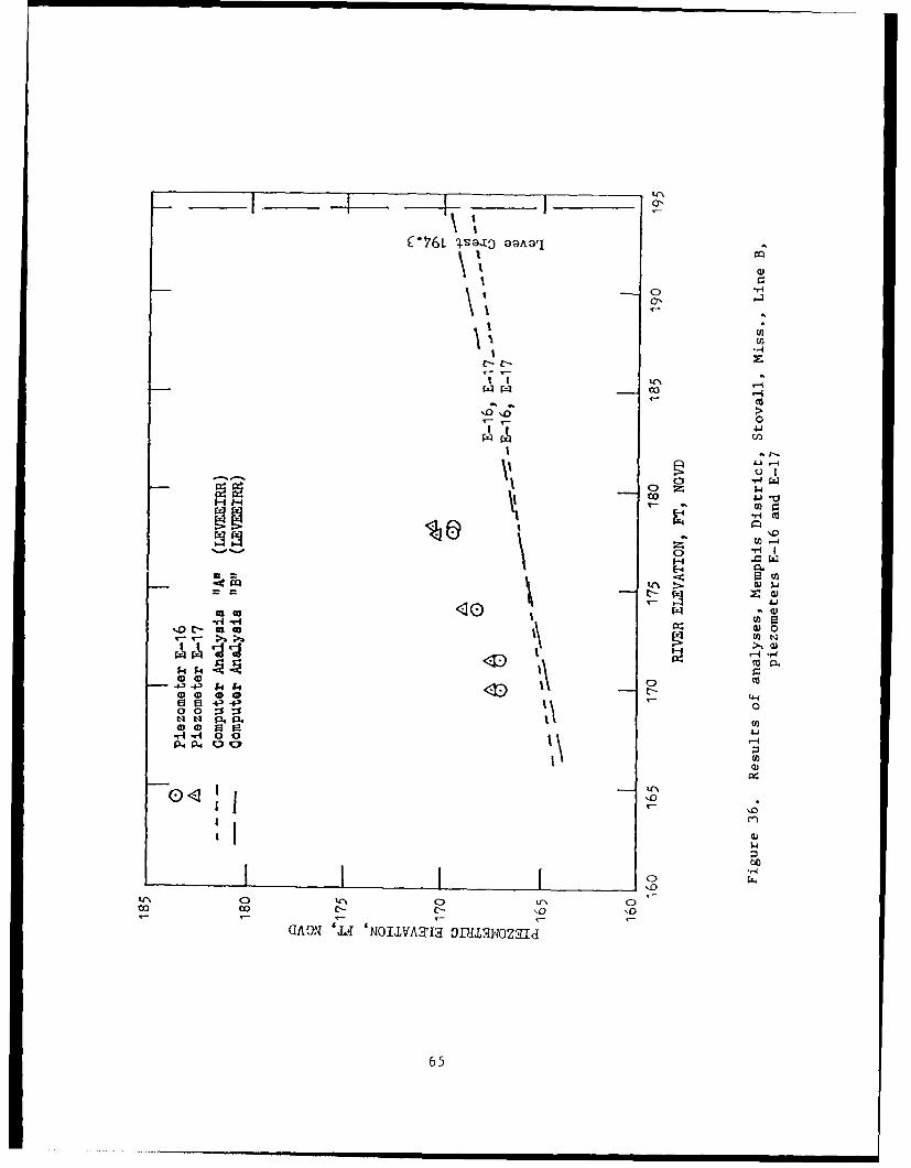
65 -
the entrance distance all had relatively little effect. A modification of
LEVEEIRR to allow different permeabilities on opposite sides of the levee may
afford a better analysis of such sections.
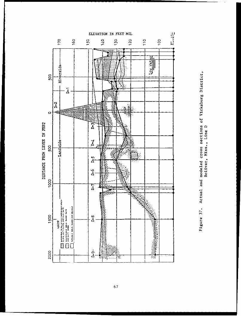
Vicksburg District,Bolivar, Miss., Line D
38. This piezometer range is located along the east bank levee of the
Mississippi River 2 miles northwest of Benoit, Miss. The river at this site
is about 8 miles from the levee; however, Bolivar Chute lies about 1,200 to
1,500 ft riverward of the levee. A line of nine piezometers, D-1 through D-9,
run perpendicular to the levee at this site. A soil profile at the piezometer
line is shown in Figure 37. Irregularities in the profile include riverside
borrow pits, landside sublevees, a landside ditch, and a massive clay-filled
abandoned channel about 1,000 to 2,000 ft landside of the levee. The effect
of this channel is to concentrate seepage between the landside levee tow and
the channel.
39. The analyses gave more weight to 1973 flood data, where available,
than 1961 data. Data for 1961 were obtained during a falling river, and an
inverse relationship between river stage and piezometric elevation was appar-
ent. Data points at higher river stages are generally 1973 data, and those at
lower stages are generally 1961 data. Data from piezometers D-1 and D-7
appears unreliable as it plots considerably lower than other piezometric data.
This may be due to the piezometer tops being founded in fine-grained blanket
materials rather than in the pervious substratum. Parameters used in the
analyses are shown in Table 6. Results of the analyses for all nine piezom-
eter locations are shown in Figures 38 through 41. A permeability ratio
(kf/kb) of 1,000 was found to provide the best fit to the observed data.
These results are labeled "Analysis A." Performance predictions for an
assumed permeability ratio of 100 are also shown (Analysis B), and it is seen
that the difference is relatively small, particularly at relatively large
distances landside of the levee.
40. Assuming a flood to the project flow line of el 166.4, a landside
tailwater of 140.5, and a permeability ratio of 1,000, a gradient at the levee
toe of 0.82 is calculated. Assuming a permeability ratio of 100 reduces the
gradient to 0.63.
66
ELEVATION IN FEET MSL4-
C4
40~
0*
co
44I Q
z ____
0 ~U) co(o)
P4J
C>C
C)4 z c
C)U
o 12)
"'( ,-A -
67
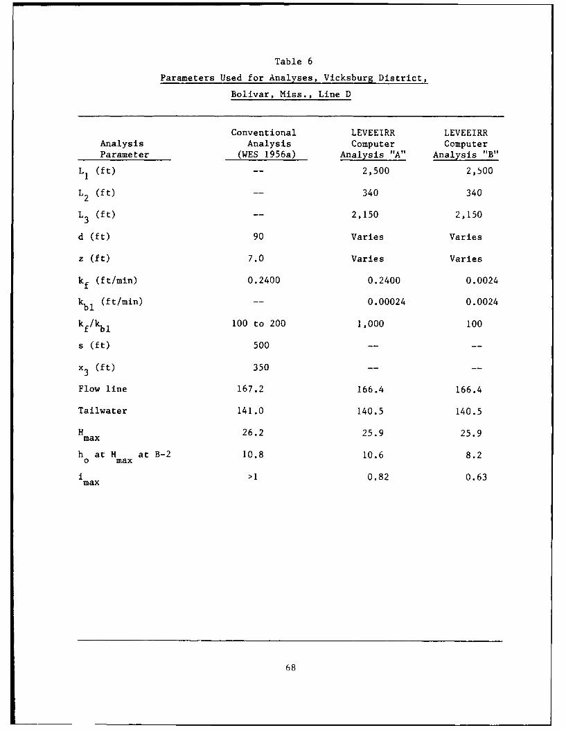
Table 6
Parameters Used for Analyses, Vicksburg District,
Bolivar, Miss., Line D
Conventional LEVEEIRR LEVEEIRRAnalysis Analysis Computer ComputerParameter (WES 1956a) Analysis "A" Analysis "B"
L (ft) 2,500 2,500
L 2 (ft) 340 340
L 3 (ft) -- 2,150 2,150
d (ft) 90 Varies Varies
z (ft) 7.0 Varies Varies
kf (ft/min) 0.2400 0.2400 0.0024
kbl (ft/min) -- 0.00024 0.0024
k1f I00 to 200 1,000 100
s (ft) 500 -- --
x3 (ft) 350 -- --
Flow line 167.2 166.4 166.4
Tailwater 141.0 140.5 140.5
H 26.2 25.9 25.9max
h at H at B-2 10.8 10.6 8.2o max
i >1 0.82 0.63max
68
00
al c.-C -
Cd ow
0 3'\ 0
0 LC'\
GAM~~~x ibONLLA IdlW~l
69o
\ -99L -10 '. l GOA0'Ia
o 0o'.0o 4J
$4:
% % $4OW
'U' * EH
0' 'U'>
0'.~ 0'0 ci''
q-4.r -H
o d
-r, 0 % . 5. 02 r.
*45.4
$i4 41
0 44
C 4,
13W0 : 0~
0. U
70
'0
1% co
wI co$'4
a\ -A'00
c -H
ii 0
\\ 13cd~
>t '
4i 4tr\4
-4 o 0 0 0
a4 0L u u
ICIE)cf
U' CON
(LO '01 NOCOT~ 0.,-4Oa
ci 71
00C-O
00
-40
4)0
cr1 a,(%c :
S.4 14
0 (D
00u
O'N 0' u
C>N C\
GADN 0~ NIVT9 IIWZ1
S-4 $~4 72
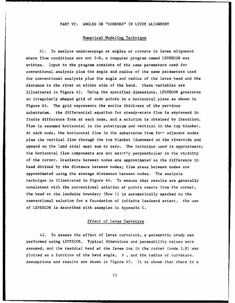
PART VI: ANGLES OR "CORNERS" IN LEVEE ALIGNMENT
Numerical Modeling Technique
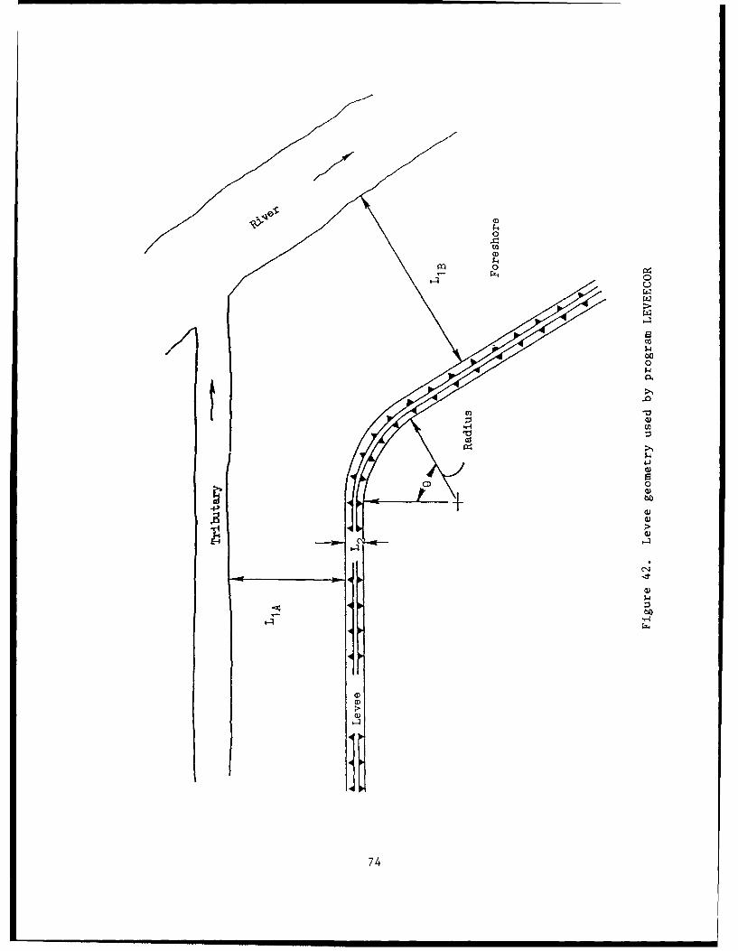
41. To analyze underseepage at angles or corners in levee alignment
where flow conditions are not 2-D, a computer program named LEVEECOR was
written. Input to the program consists of the same parameters used for
conventional analysis plus the angle and radius of the same parameters used
for conventional analysis plus the angle and radius of the levee bend and the
distance to the river on either side of the bend. these variables are
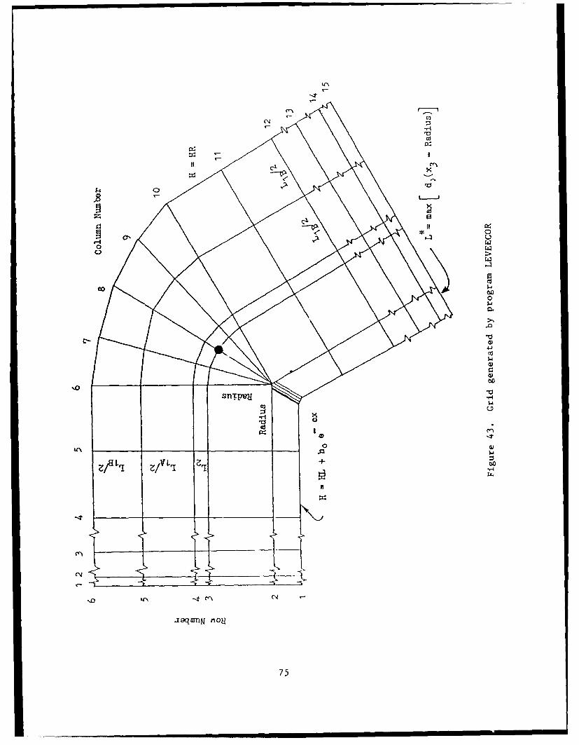
illustrated in Figure 42. Using the specified dimensions, LEVEECOR generates
an irregularly shaped grid of node points in a horizontal plane as shown in
Figure 43. The grid represents the entire thickness of the pervious
substratum. the differential equation for steady-state flow is expressed in
finite difference form at each node, and a solution is obtained by iteration.
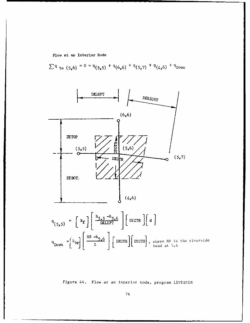
Flow is assumed horizontal in the substratum and vertical in the top blanket.
At each node, the horizontal flow in the substratum from fo,' adjacent nodes
plus the vertical flow through the top blanket (downward on the riverside and
upward on the land side) must sum to zero. The technique used is approximate;
the horizontal flow components are not exi.ty perpendicular in the vicinity
of the corner. Gradients between nodes are approximated as the difference in
head divided by the distance between nodes; flow areas between nodes are
approximated using the average distances between nodes. The analysis
technique is illustrated in Figure 44. To ensure that results are generally
consistent with the conventional solution at points remote from the corner,
the head at the landside boundary (Row 1) is automatically matched to the
conventional solution for a foundation of infinite landward extent. the use
of LEVEECOR is described with examples in Appendix C.
Effect of Levee Curvature
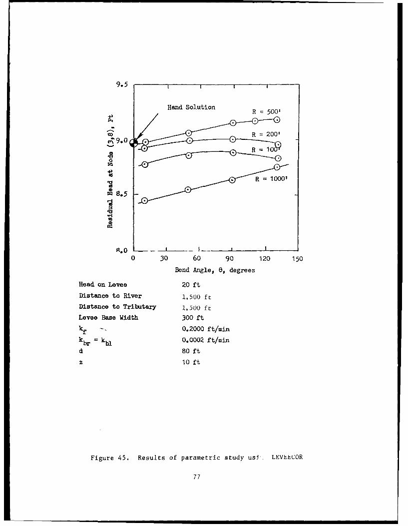
42. To assess the effect of levee curvature, a parametric study was
performed using LEVEECOR. Typical dimensions and permeability values were
assumed, and the residual head at the levee toe in the corner (node 3,8) was
plotted as a function of the bend angle, 6 , and the radius of curvature.
Assumptions and results are shown in Figure 45. It is shown that there is a
73
00
CD 0
4)
4)
74
IC'
q::(
14 0
Ct
0
00
0w
"-4
IC~ __ _____ ___to
?/ ri II "-
75
Flow at an Interior Node
Eq to (5,6) 0 q(5,5) + q(6,6 ) + q(5,7) + q(4,6) + qDown
IJZRIGH7T
(6,6)
DXC (5,7)
DYBOT
J (4p6)
q( ) kf. [ h5*.-h5.6 DYCTR]dJ
q brl] 1 [~ uiT YCR weeH is the riversideDwn DZCJ R head at 5,6
Figure 44. Flow at an interior node, program LEVEECOR
76
9.5
Hand Solution R=50
to R=20
.0
0
R000
S8.5
ri
U:
0 30 60 90 120 150
Bend Angle, 03, degrees
Head on Levee 20 ft
Distance to River 1,500 ft
Distance to Tributary 1,.s00 ft
Levee Base Width 300 ft
kf --- 0.2000 ft/min
k b =kb 0.0002 ft/mmn
d 80 ft
z 10 ft
Figure 45. Results of parametric study usJi. LEVtEECOR
77

tendency for the residual head to increase with increasing bend angle, but the
increase is relatively small, less than 0.5 ft for the example investigated.
Effects may be more pronounced for shorter entrance distances, different
permeability ratios, etc; however, time did not afford a complete investiga-
tion of evety parameter. As the radius was increased to 500 ft, the head
increased; the head decreased after the radius exceeded this value. Such
variation may be related to the fact that the model geometry changes as the
radius changes. Ideally, all the curves should pass through the point labeled
"hand solution"; however, discrepancies arise because the numerical solutions
for different radii generate different grid geometries. Some degradation of
results is apparent for relatively large and small radii and for bend angles
greater than 90 deg.
43. Although the study seems to indicate that the bend angle may have
only a slight effect on the residual head for a symmetric problem, the program
LEVEECOR should be useful for analysis of asymmetric problems because of its
ability to model different distances to the river on either side of the bend.
LEVEECOR should be used for radii greater than 500 ft since the model failed
to produce reasonable trends or agree with the closed form solution.
Actual Versus Predicted Performance
44. The program LEVEECOR was used to analyze a set of corner reaches
where piezometric data were available. Performance predictions obtained from
the program were compared to predictions based on conventional analysis and to
actual piezometer readings. A discussion of these analyses and results
follows.
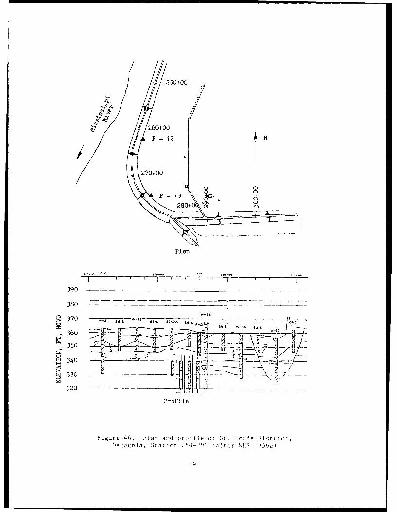
St. Louis District,Degognia, Station 260-290
45. This piezometer range is located in the Degognia Levee and Drainage
District adjacent tc a near-right-angle bend in the Mississippi River called
Liberty Bend. A plan of the levee and a foundation profile are shown in Fig-
ure 46. On the upstream side of the bend, the Misbissippi River is about
650 ft from the levee. On the downstream side of the bend, a chute separates
the floodplain from Wilkinson ITslnd, and the Mississippi River is uii LIke
opposite sided of the island. Underseepage performance at this location dur-
ing the 1973 flood was described by the USAFI), St. Louis (1976).
78
250+00
-VIII I
.414
Al
-'-V 260+00
P-12 N
270+00
0P-13 013
28Q+-0 g0
Plan
390
380370 W--3-
3-I 58- SO7-5 57-36 6- W- 7 -
36 __
~350340
S330 _
320
Profile
Figure 46. Plan and profile oi St, l.ouLs District,
D)egogn fa, Stat ion 260-2)() 'nfter VE.S 95,a)
79
Piezometer P-12 at the upstream end of the bend flowed over a 4-ft extension;
the estimated head exceeded 5.2 ft, and the estimated gradient exceeded 0.43.
46. Three analyses were performed, one using the conventional method
and two using the program LEVEECOR: analysis assumptions are summarized in
Table 7. The conventional analysis is based on parameters obtained and
inferred from TM 3-430 (WES 1956b). The permeability ratio for the conven-
tional analysis was reduced from 1,000 to 500 to better fit the observed data.
The entrance distance of 1,000 ft is a judgmental average of the widely vary-
ing distances on either side of the bend. Computer analysis "A" was performed
using the same permeability ratio as the conventional analysis, but the dis-
tances to the river, LIA and LIB, represent prototype conditions. For com-
puter analysis "B" the permeability ratio was varied to get the best match
with the observed data. Performance predictions from the three analyses are
compared to observed data in Figure 47. For the dimensions modeled, it was
found that a permeability ratio of 150 provided the best match to observed
performance. Using the program LEVEECOR provides a convenient method for
back-calculating the permeability ratio in this case where an appropriate
single value for the distance to the river required for conventional analysis
is difficult to assess.
St. Louis District,East Cape, Station 94
47. This piezometer range is located at an abrupt 50-deg bend at Sta-
tion 94 of the East Cape Girardeau levee, which is across the river from Cape
Girardeau, Mo. The data used are from the 1973 flood and were previously
analyzed by USAED, St. Louis (1976). A plan view and foundation profile are
shown in Figure 48.
48. Three analyses were performed; assumptions are summarized in
Table 8. The conventional analysis is based on parameters obtained and
inferred from TM 3-430 (WES 1956b). Computer aioayzis "A" was performed using
the same permeability ratio as the conventional analysis, but the geometry is
more completely described. For computer analysis "B" the same geometry was
used, but the permeability ratio was varied to get the buc=t match with the
observed data. Performance predictions from the three analy.es are compared
to observed data in Figure 49. Tt was found that the permeability ratio had
to be lowerel to 25 to match observed performance. The VSAED, St. Louis
(1976) reported that numerous pin boils were present in the fields landside of
b C
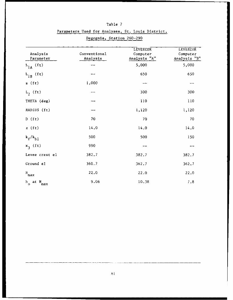
Table 7
Parameters Used for Analyses, St. Louis District,
Degognia, Station 260-290
LEVEECOR LEVEECORAnalysis Conventional Computer ComputerParameter Analysis Analysis "A" Analysis "B"
L1A (ft) -- 5,000 5,000
LIB (ft) -- 650 650
s (ft) 1,000 -- --
L2 (ft) -- 300 300
THETA (deg) -- 110 110
RADIUS (ft) -- 1,120 1,120
D (ft) 70 70 70
z (ft) 14.0 14.0 14.0
kfl/kbl 500 500 150
x3 (ft) 990 -- --
Levee crest el 382.7 382.7 382.7
Ground el 360.7 362.7 362.7
H 22.0 22.0 22.0maxh at H 9.06 10.38 7.8o max
• , ,a a t I 81
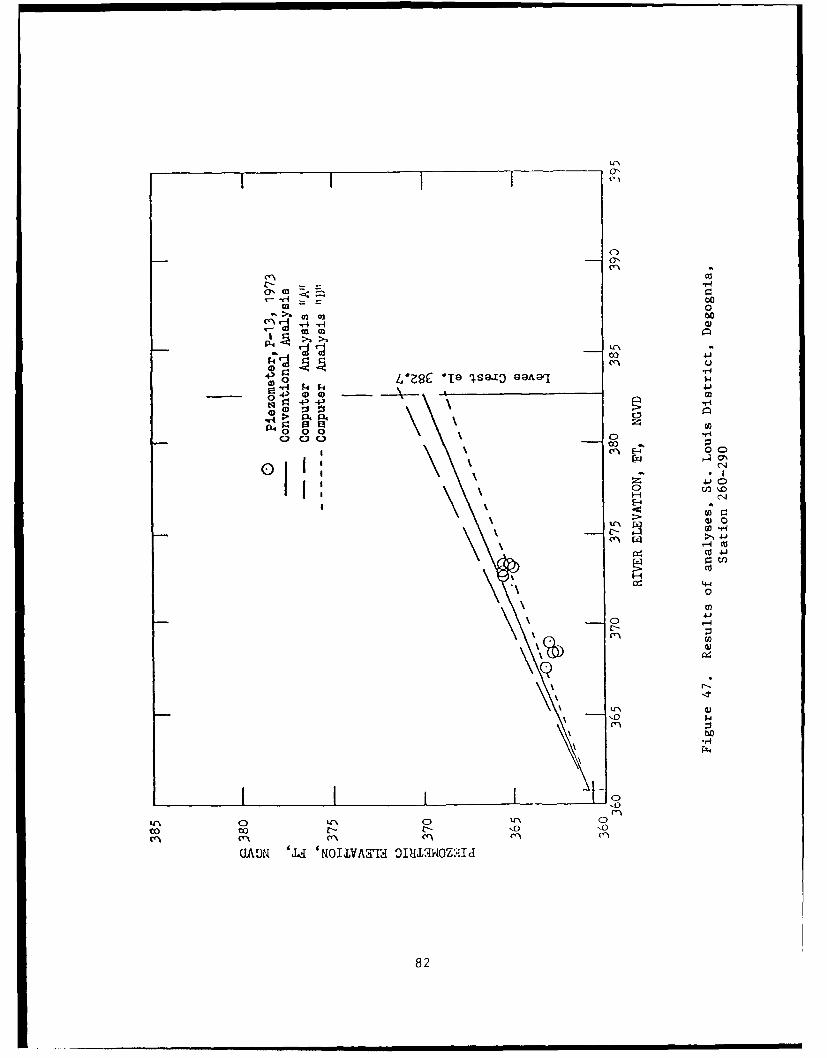
Cl\d
0"~ 0
0200
CC\~ \ \5.1
r:4--(D V 0
0
E 0 0>
U)~(3 COC- 00 -H
~~~~M~> 4OJA-J3fU~O~
82 c
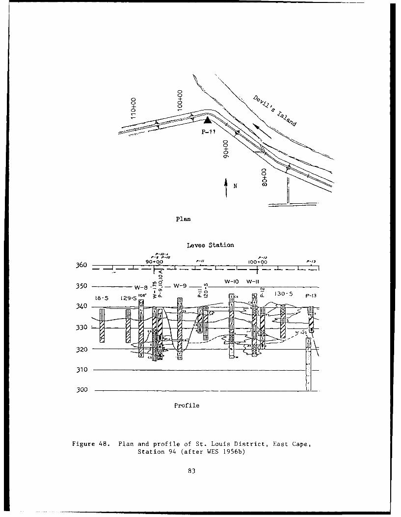
00
4N 0 __ __
Plan
Levee Station
-vP-IoA-A
360 90+OP 100+00 P-13
d 0 w-10 w-11350 ___ ___ -t- ____9__ ___,_ __N
18-5 129-S 106 , CLa 2 s sP
3100
320
310
300 A
Profile
Figure 48. Plan and profile of St. Louis District, East Cape,Station 94 (after WES 1956b)
83
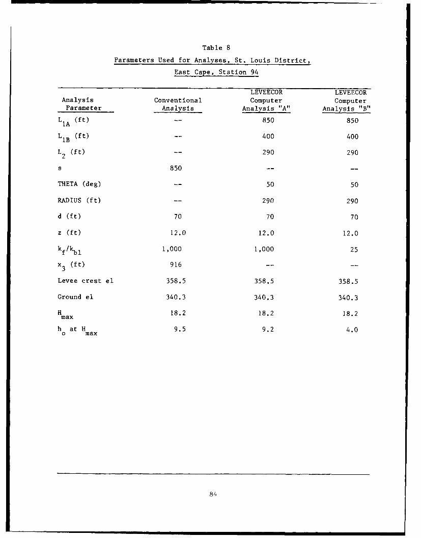
Table 8
Parameters Used for Analyses, St. Louis District,
East Cape, Station 94
LEVEECOR LEVEECORAnalysis Conventional Computer ComputerParameter Analysis Analysis "A" Analysis "B"
L1A (ft) -- 850 850
L1B (ft) -- 400 400
L2 (ft) -- 290 290
s 850 -- --
THETA (deg) -- 50 50
RADIUS (ft) -- 290 290
d (ft) 70 70 70
z (ft) 12.0 12.0 12.0
kf kbl 1,000 1,000 25
x 3 (ft) 916 -- --
Levee crest el 358.5 358.5 358.5
Ground el 340.3 340.3 340.3
H 18.2 18.2 18.2max
h at H 9.5 9.2 4.0O max
84
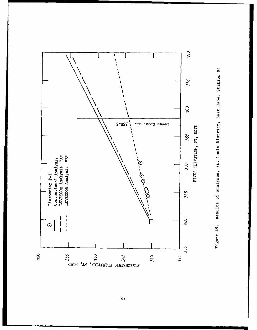
0C-
100
co
Clw
E-4
a3 0
o0 0 co
4-l 0 04 0oAO 'C4 'N0V3I co1~aO
> 10) fI CI85

this location. These observations are consistent with the unusually low
permeability ratio indicated.
86
PART VII: CONCLUSIONS AND RECOMMENDATIONS
Conclusions
49. The "conventional method" of underseepage analysis is restricted to
the special case of foundations consisting of two layers, each of uniform
thickness and with horizontal boundaries. For this special case, there is a
closed-form solution for the governing differential flow equation. Where
actual foundation conditions are complex, considerable engineering judgment
must be used to assign equivalent or "effective" values for the parameters
describing the foundation geometry. Analysis results can be very dependent on
the judgments made and may vary considerably among different engineers analyz-
ing the same soil profile. Using numerical methods and microcomputers, the
differential equation can be solved for more general cases of foundation and
levee geometry. This reduces uncertainty introduced in the analysis regarding
the geometry and allows the analyst to focus on the effects of other vari-
ables, in particular the material permeabilities and landside water
elevations.
50. Three microcomputer programs were developed to perform underseepage
analysis for three special cases of foundation conditions that are representa-
tive of many locations in the Mississippi Valley. Using these programs, pre-
dictions of piezometric head were made and compared to observed piezometric
data at eight locations. The field permeability ratios were estimated by
varying values of the program input parameters until predictions matched
observed performance. Although the programs were evaluated by reanalyzing
past performance, they would be equally useful for new analyses. Because grid
size effects on the numerical solution were not parametrically investigated
the grid size cannot be varied by the user, the reader is cautioned that
exit gradients computed by these programs may not be conservative. Experi-
ences with the programs and findings from these studies are summarized below.
Foundations charac-terized by three layers
51. Where foundation sands are significantly different in the upper and
lower parts of the substratum, a three-layer model provides a more consistent
or general representation of prevailing conditions than the conventional two-
layer analysis. The program LEVEE3L allows modeling of such conditions and
87
allows for different vertical and horizontal permeabilities in each of the
three layers. Some of the effects of variations in the middle stratl.m have
been demonstrated by parametric studies.
52. The program LEVEE3L should be useful to predict underseepage condi-
tions where three-layer conditions are known to exist and reasonable estimates
can be made of the six required permeabilities. A second case of a three-
layer foundation not studied herein is the case of a sandy or silty top
blanket overlying a clay layer. LEVEE3L would be applicable to such condi-
tions. Because of its ability to account for six permeabilities, LEVEE3L is
less useful for back-calculation of permeability values or ratios because five
values must be assumed to calculate the sixth.
53. The analysis at Sny Island illustrates how a thin top blanket of
clay overlying a silty middle stratum can lead to boils while piezometers at
the base of the middle stratum indicate only moderate residual heads.
54. The analysis at Eutaw, Miss., illustrates that irregularities in
the elevations and thicknesses of the soil deposits may dominate the problem
more than the effect of the middle layer. Assigning appropriate effective
ground elevations may be critical to accurately predict landside heads, and
these elevations may differ significantly at different points along the
profile.
Foundations characterizedby two layers of irregular shape
55. Using conventional analysis techniques, the calculated residual
head is a function of both the assumed equivalent geometry and the perme-
ability ratio. Calculated residual heads may be highly uncertain because of
the uncertainty introduced in the representation of foundation geometry.
Using the program LEVEEIRR, a two layer foundation geometry can be represented
as precisely as it is known. Thus, the permeability values and ratio can be
isolated as the independent variables. The program is applicable to many
common conditions of irregular foundation geometry, including borrow pits,
ditches, and clay-filled channels. It should be particularly useful in
assessing the impact of proposed changes adjacent to levees, such as construc-
tion of new ditches or elargement of borrow areas, problems that commonly
occur and are not conveniently assessed using conventional methods. A partic-
ularly useful feature of LEVEEIRR is its capability to predict or assess per-
formance (residual head and gradient) at any desired distance from the levee
88
or any piezometer location by appropriate specification of segment boundaries.
In the author's opinion, LEVEEIRR probably has the greatest pctential of the
three programs for extensive use in routine practice.
56. The above comments on calculating residual heads apply as well to
back-calculation of permeability ratios from observed residual heads. As the
foundation geometry can be precisely described using LEVEEIRR, back-calculated
permeability values should be more reliable than those related to "trans-
formed" geometry.
Angles or "corners" in levee alignment
57. Using program LEVEECOR, underseepage conditions at bends in levee
alignment or levee corners can be analyzed. Because of the problem complex-
ity, the program employs more approximations than the other two programs. For
typical problems investigated, the increase in residual head due to the corner
effect is relatively small, typically less than a foot. This effect alone
would not seem to warrant using the program in lieu of conventional methods.
However, the program may be useful in practice because it allowF the analyst
to model actual distances to the river on either side of levee rather than
assuming an "effective distance" that somehow averages widely different condi-
tions. LEVEECOR should be used with caution, particularly for radii less than
500 ft since the model failed to produce reasonable trends or agree with the
closed form solution in that range.
Permeability ratios
58. Permeability ratios cannot be reliably back-calculated usng
LEVEE3L. Back-calculated permeability ratios obtained using LEVEEIRR and
LEVEECOR varied from 25 to 1,000 and were typically 500 or less. The low
ratio of 25 at East Cape was for a site where pin boils were occurring, indi-
cating that the apparently high top blanket permeability was due to open path-
ways or defects in the blanket. For the most part, the ratios calculated
using the programs were consistent with those obtained by experienced analysts
using conventional analysis. However, the programs allow a less experienced
analyst to model the geometry and foundation conditions as they are perceived
without the assignment of effective dimensions.
Comparison of programs and results
59. The three programs and the conventional method were used to analyze
a common problem, and the results are compared in Appendix D. Variation among
the solutions for the problem analyzed was several feet, a range somewhat
89
larger than expected at the outset of the research. Some reasons for the
variation are suggested in the appendix, they include the use of fundamentally
different assumptions in deriving the flow equations and truncation error. It
is expected that some of this variation could be reduced by using finer grids
or higher order approximations for the derivatives. Such improvements would
require a second iteration in program development. The intent of the present
research was to demonstrate the applicability of special-purpose microcomputer
programs (as compared with general-purpose computer programs) for the problems
of interest. Based on the parametric studies performed and the case histories
analyzed, it is be'±eved that the present versions of the programs are suit-
able and should be recommended for comparison studies to evaluate the effects
of borrow areas, ditches, varying permeabilities, etc.
Recommendations
60. Based in the results of this research, the following recommenda-
tions are made:
a. The developed programs should be used as a supplement to con-ventional analysis where geometry warrants.
b. Modifications should be made to LEVEE3L to provide for variablegrid spacing.
c. Assuming that LEVEEIRR would be the most used of the threeprograms, improvements should be made to allow for differentlandside and riverside blanket permeabilities, to provide forexpedient data input and file building, to provide a graphicdisplay of foundation geometry, and to provide for more thanone landside water level.
d. A three-layer version of LEVEEIRR should be developed thatincorporates features of LEVEE3L.
e. By analyzing additional reaches and systematically assessingall results, better guidelines should be developed for estimat-ing the field permeability ratio as a function of materialtypes and thicknesses.
f. The extension of the programs to analyze reaches where reliefwells are present should be investigated.
. The programs should be field tested to determine the need foradditional changes and improvements.
90
REFERENCES
Bennett, P. T. 1946. "The Effect of Blankets on the Seepage through PerviousFoundations," Transactions, American Society of Civil Engineers, Vol 111,p 215.
Cunny, R. W. 1980. "Documentation and Analysis of Rock Island UnderseepageData," Technical Report GL-80-3, US Army Engineer Waterways Experiment
Station, Vicksburg, Miss.
McClelland Engineers, Inc. 1958. "Investigation of Underseepage and ItsControl, Lower Mississippi River Levees, Appendix F: Analysis of 1973Piezometric Data," Technical Memorandum No. 3-424, Report to US Army Corps ofEngineers, Vicksburg District, Vicksburg, Miss.
Tracy, F. T. 1973. "A Plane and Axisymmetric Finite Element Program forSteady State and Transient Seepage Problems," Miscellaneous Paper K-73-4, USArmy Engineer Waterways Experiment Station, Vicksburg, Miss.
United States Army Engineer District, St. Louis. 1976. "Reevaluation ofUnderseepage Controls, Mississippi River Levees, Alton to Gale, IL, Phase I:Performance of Underseepage Controls During the 1973 Flood," St. Louis, Mo.
US Army Engineer Waterways Experiment Station. 1956a. "Investigation ofUnderseepage and Its Control, Lower Mississippi River Levees," TechnicalMemorandum 3-424, Vicksburg, Miss.
• 1956b. "Investigation of Underseepage and Its Control, LowerMississippi River Levees, St. Louis District, Alton to Gale, IL" TechnicalMemorandum 3-430, Vicksburg, Miss.
• 1964. "Investigation of Underseepage and Its Control, LowerMississippi River Levees, Appendix E: Analysis of 1961 Piezometric Data,"Technical Memorandum 3-424, Vicksburg, Miss.
US Army, Office, Chief of Engineers. 1978. "Design and Construction ofLevees," Engineer Manual EM 1110-2-1913, Washington, DC.
Wolff, T. F. 1986. "Design and Performance of Underseepage Controls: ACritical Review," unpublished report prepared for US Army Engineer WaterwaysExperiment Station by Michigan State University, East Lansing, Mich.
91
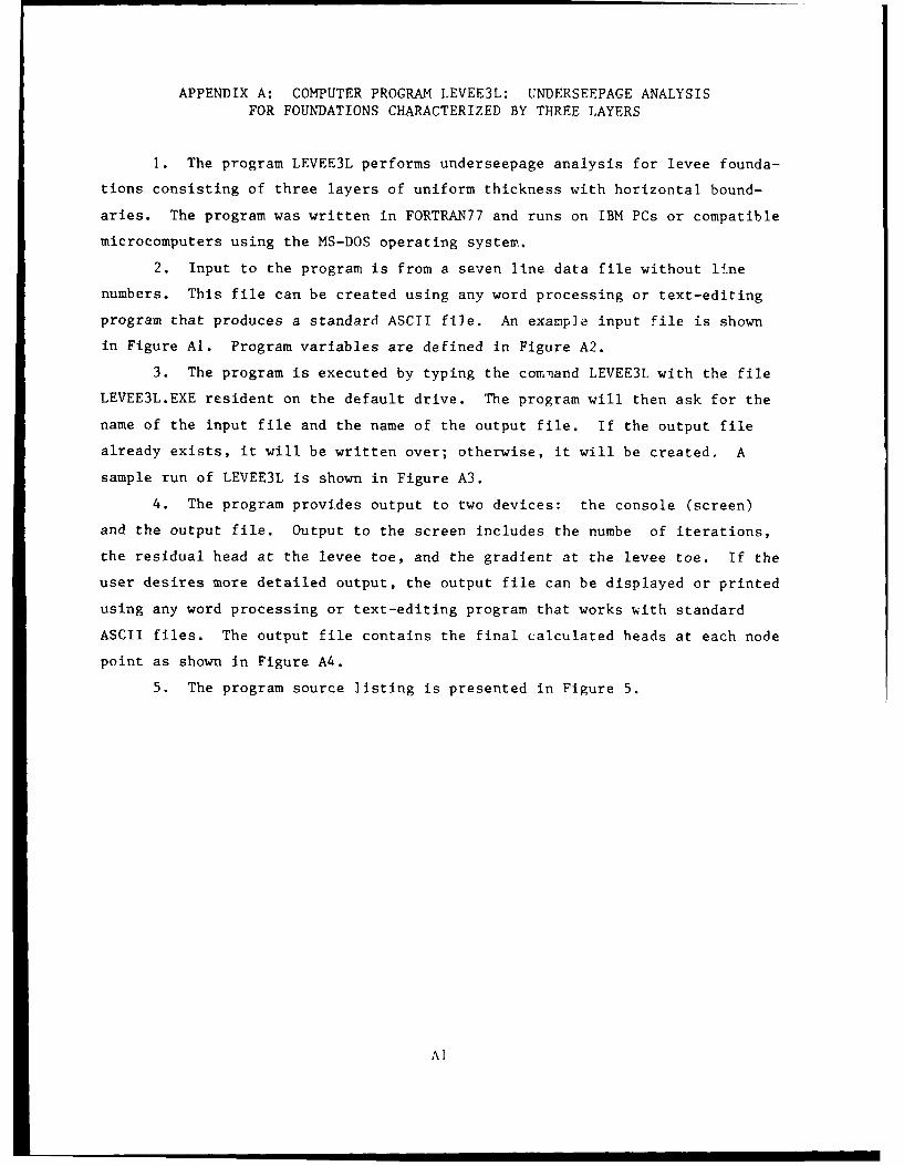
APPENDIX A: COMPUTER PROGRAM LEVEE3L: UNDERSEEPAGE ANALYSISFOR FOUNDATIONS CHARACTERIZED BY THREE LAYERS
1. The program LEVEE3L performs underseepage analysis for levee founda-
tions consisting of three layers of uniform thickness with horizontal bound-
aries. The program was written in FORTRAN77 and runs on IBM PCs or compatible
microcomputers using the MS-DOS operating system.
2. Input to the program is from a seven line data file without line
numbers. This file can be created using any word processing or text-editing
program that produces a standard ASCII file. An example input file is shown
in Figure Al. Program variables are defined in Figure A2.
3. The program is executed by typing the comnand LEVEE3L with the file
LEVEE3L.EXE resident on the default drive. The program will then ask for the
name of the input file and the name of the output file. If the output file
already exists, it will be written over; otherwise, it will be created. A
sample run of LEVEE3L is shown in Figure A3.
4. The program provides output to two devices: the console (screen)
and the output file. Output to the screen includes the numbe. of iterations,
the residual head at the levee toe, and the gradient at the levee toe. If the
user desires more detailed output, the output file can be displayed or printed
using any word processing or text-editing program that works with standard
ASCII files. The output file contains the final calculated heads at each node
point as shown in Figure A4.
5. The program source listing is presented in Figure 5.
AI

EXAMPLE INPUT FILE FOR LEVEE3L
Values Variable Names
Example Problem TITLE
20.00 0.00 HR, HL
1000.00 50.00 3000.00 LI, L2, L3
10.0 20.0 60.0 ZI, Z2, D
.0002 0.0100 0.0400 KV1, KV2, KV3
.00100 0.0500 0.2000 KH1, KH2, KH3
.005 500 TOL TRIES
)les are defined as follows:
iescriptive title for the problem (80 characters maximum).
distance from the riverside levee toe to the river or an open
ntrance.
distance from the riverside levee toe to the landside levee toe.
distance from the landside levee toe to an open seepage exit. This
very long (e.g. twice the effective exit distance) when modeling
ns of infinite extent.
elevation of water on the riverside of the levee. If the landside
landside ground is taken as the datum, HR is the net head on the
elevation of water on the landside of the levee or the elevation of
ground if no water is present. This level is often taken as the
which case HL is 0.0.
thickness of the top blanket in feet or any consistent units.
thickness of the middle stratum in feet or any consistent units.
Figure Al. Example input file, program LEVEE3L (Continued)
A2
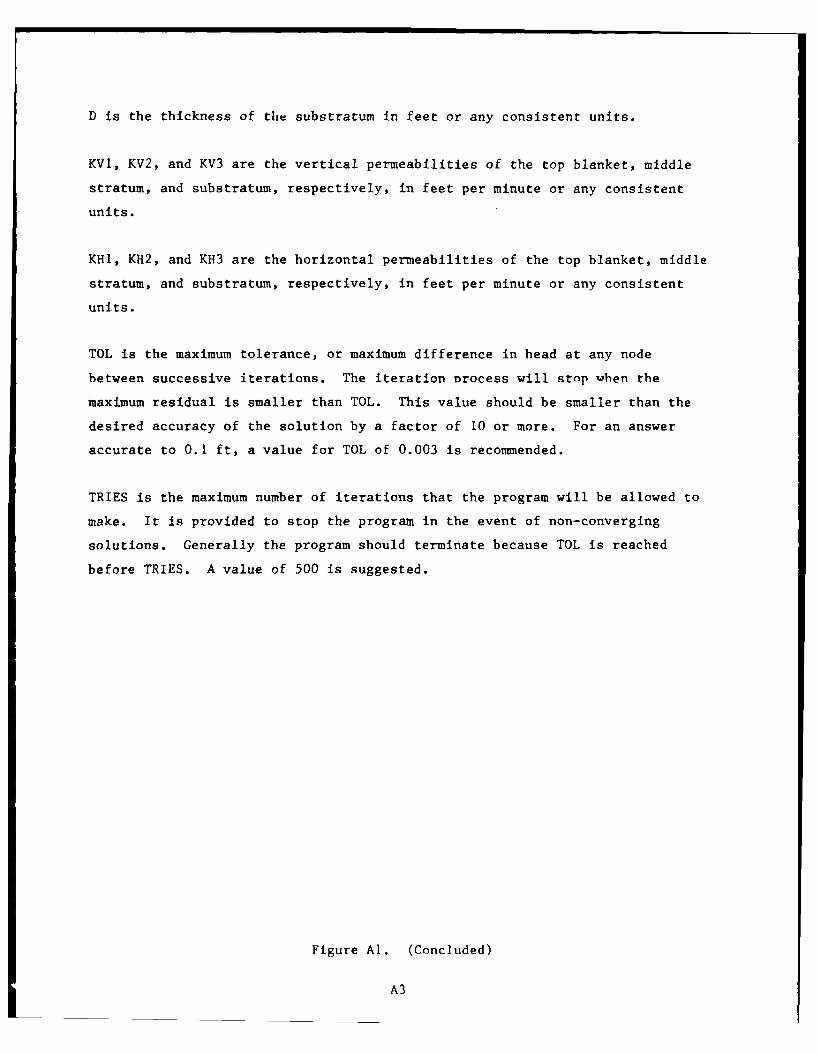
D is the thickness of the substratum in feet or any consistent units.
KVI, KV2, and KV3 are the vertical permeabilities of the top blanket, middle
stratum, and substratum, respectively, in feet per minute or any consistent
units.
KHl, KH2, and KH3 are the horizontal permeabilities of the top blanket, middle
stratum, and substratum, respectively, in feet per minute or any consistent
units.
TOL is the maximum tolerance, or maximum difference in head at any node
between successive iterations. The iteration nrocess will stop when the
maximum residual is smaller than TOL. This value should be smaller than the
desired accuracy of the solution by a factor of 10 or more. For an answer
accurate to 0.1 ft, a value for TOL of 0.003 is recommended.
TRIES is the maximum number of iterations that the program will be allowed to
make. It is provided to stop the program in the event of non-converging
solutions. Generally the program should terminate because TOL is reached
before TRIES. A value of 500 is suggested.
Figure Al. (Concluded)
A3
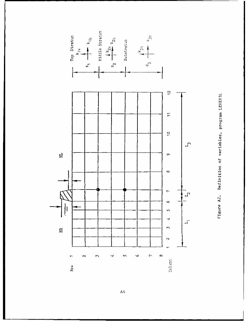
444) ~ A
Ua)A ft
~(N
:11
I~ IA 10 c
A4-
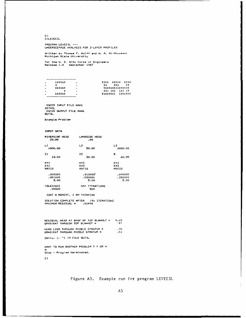
C>
C>LEVEE3L
PROGRAM LEVEESL ---
UNDERSEEPAGE ANALYSIS FOR 3-LAYER PROFILES
Written by Thomas F. Wolff and H. A. Al-Moj.64.1
Michigan State University
For the U. S. Army Corps of EngineersRelease 1.0 September 1987
XXXXXX XXXX XXXXX XXXXx XX XXX xxXXXXXX XXXXXXXIIXXXXXX
S.XXI [XI IXI IXXXXXXX XXXXXXXI IXXXXXX
ENTER INPUT FILE NAMEDATA3LENTER OUTPUT FILE NAMEOUT3L
Example Problem
INPUT DATA
RIVERSIDE HEAD LANDSIDE HEAD20.00 .00
LI L2 L31000.00 50.00 3000.00
ZI Z2 D10.00 20.00 60.00
KYI KY2 KY3KXI KX2 KX3RATIO RATIO RATIO
.000200 .010006 .040000
.001000 .050000 .2000005.00 5.00 5.00
TOLERANCE MAX ITrRA'IONS.00500 500
JUST A MOMENT, I AM THINKING
SOLUTION COMPLETE AFTER 191 ITERATIONSMAXIMUM RESIDUAL - .00498
RESIDUAL HEAD AT BASF OF TOP BLANKET - 9.601
GRADIENT THROUGH TOP BLANKET - .97
HEAD LOSS THROUGH MIDDLE STRATUM .35
GRADIENT THROUGH MIDDLE STRATUM - .02
OUl* . , IN FILE OUT3L
WANT TO RUN ANOTHER PROBLEM 7 Y OR N
NStop - Program terminated.
C>
Figure A3. Example run for program LEVEE3L
A5
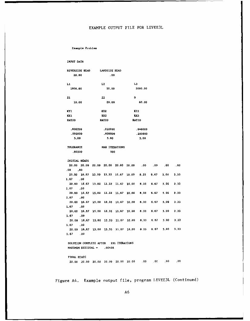
EXAMPLE OUTPUT FILE FOR LEVEE3L
Example Problem
INPUT DATA
RIVERSIDE HEAD LANDSIDE OEAD
20.00 .00
Li L2 L3
1000.00 50.00 3000.00
Zi Z2 D
10.00 20.00 60.00
KI KY2 KY3
KXl KX2 XX3
RATIO RATIO RATIO
.000200 .010000 .040000
.001000 .050000 .200000
5.00 5.00 5.00
TOLERANCE MAX ITERATIONS
.00500 500
INITIAL READS
20.00 20.00 20.00 20.00 20.00 20.00 .00 .00 .00 .00
.00 .00
20.00 16.67 15.00 13.33 11.67 10.00 8.33 6.67 5.00 3.33
1.67 .00
20.00 16.67 15.00 13.33 11.67 10.00 8.33 6.67 5.00 3.33
1.67 .00
20.00 16.67 15.00 13.33 11.67 10.00 8.33 6.67 5.00 3.33
1.67 .00
20.00 16.67 15.00 13.33 11.67 10.00 8.33 6.67 5.00 3.33
1.67 .00
20.00 16.67 15.00 13.33 11.67 10.00 8.33 6.67 5.00 3.33
1.67 .00
20.00 16.67 15.00 13.33 11.67 10.00 8.33 6.67 5.00 3.33
1.67 .00
20.00 16.67 15.00 13.33 11.67 10.00 8.33 6.67 5.00 3.33
1.67 .00
SOLUTION COMPLETE AFTER 191 ITERATIONS
MAXIMUM RESIDUAL - .00498
FINAL HEADS
20.00 20.00 20.00 20.00 20.00 20.00 .00 .00 .00 .00
Figure A4. Example output file, program LEVEE3L (Continued)
A6
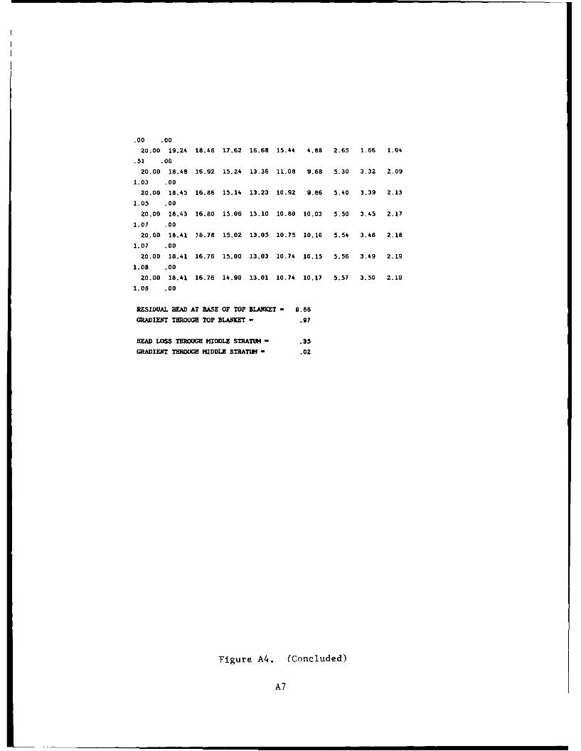
.00 .00
20.00 19.24 18.46 17.62 16.68 15.44 4.88 2.65 1.66 1.04
.51 .00
20.00 18.48 16.92 15.24 13.36 11.08 9.68 5.30 3.32 2.09
1.03 .00
20.00 18.45 16.86 15.14 13.23 10.92 9.86 5.40 3.39 2.13
1.05 .00
20.00 18.43 16.80 15.06 13.10 10.80 10.03 5.50 3.45 2.17
1.07 .00
20.00 18.41 16.78 15.02 13.05 10.75 10.10 5.54 3.48 2.18
1.07 .00
20.00 18.41 16.76 15.00 13.03 10.74 10.15 5.56 3.49 2.19
1.08 .00
20.00 18.41 16.76 14.99 13.01 10.74 10.17 5.57 3.50 2.19
1.08 .00
RESIDUAL BEAD AT BASE OF TOP BLANKET - 9.68
GRADIENT THROUGH TOP BLANKET - .97
HEAD LOSS THROUGH MIDDLE STRATUM - .35
GRADIENT THROUGH MIDDLE STRATUM - .02
Figure A4. (Concluded)
A7
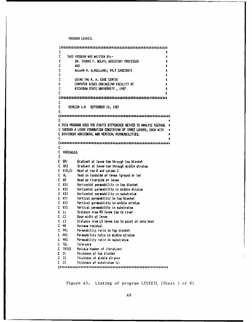
PROGRAM LEVEE3L
CS$$$$$S$S$$$$S$$$$$ISS$$S$$$$$$$ss$S$Sss$$$S$$sS$$ssss sS$s$
C SC THIS PROGRAM WAS WRITTEN BY:- $C DR. THOMAS F. NOLFFI ASSISTANT PROFESSOR $C AND $C HhAAN M. ALMOUS3AWII PH.D CANDIDATE $C $C USING THE A. H. CASE CENTER $C COMPUTER AIDED ENSINEEING FACILITY AT $C MICHIGAN STATE UNIVERSITY , 1987 $C $C$$$$$$$$$$$$$$$$$$$$$$$$$$$$$$$$$$$$$$$$$$$$$$SS$St$$$$$$$$
CC VERSION 1.0 SEPTEMBER 10, 1987C
CC THIS PROGRAM USES THE FINITE DIFFERENCE METHOD Ta ANALYZE SEEPAGE *C THROUGH A LEVEE FOUNDATION CONSISTING OF THREE LAYERS, EACH WITH #C DIFFERENT HORIZONTAL AND VERTICAL PERMEABILITIES. *C
CC VARIABLESCC SRI Gradient at levee toe through top blanketC GR2 Gradient at levee toe through middle stratumC H(R,C) Head at row R and column CC HL Head on landstde of levee (ground or tv)C HR Head on riverside of leveeC KXI Horizontal permeability in top blanketC KX2 Horizontal permeability in middle stratumC KX3 Horizontal permeability in substratumC KYI Vertical permeability in top blanketC KY2 Vertical permeability in middle stratumC KY3 Vertical permeability in substratumC LI Distance from RS levee toe to riverC L2 Base width of leveeC L3 Distance Irom LS levee toe to point of zero headC MR Maximum residualC PRI Permeability ratio in top blanketC PR2 Permeability ratio in middle stratumC PR3 Permeability ratio in substratum
C TOL ToleranceC TRIES Maximua number of iterationsC it Thickness of top blanketC 12 Thickness of middle stratu;C 13 Thickness of substratum (6)
Figure A5. Listing of program LEVEE3L (Sheet 1 of 8)
A8
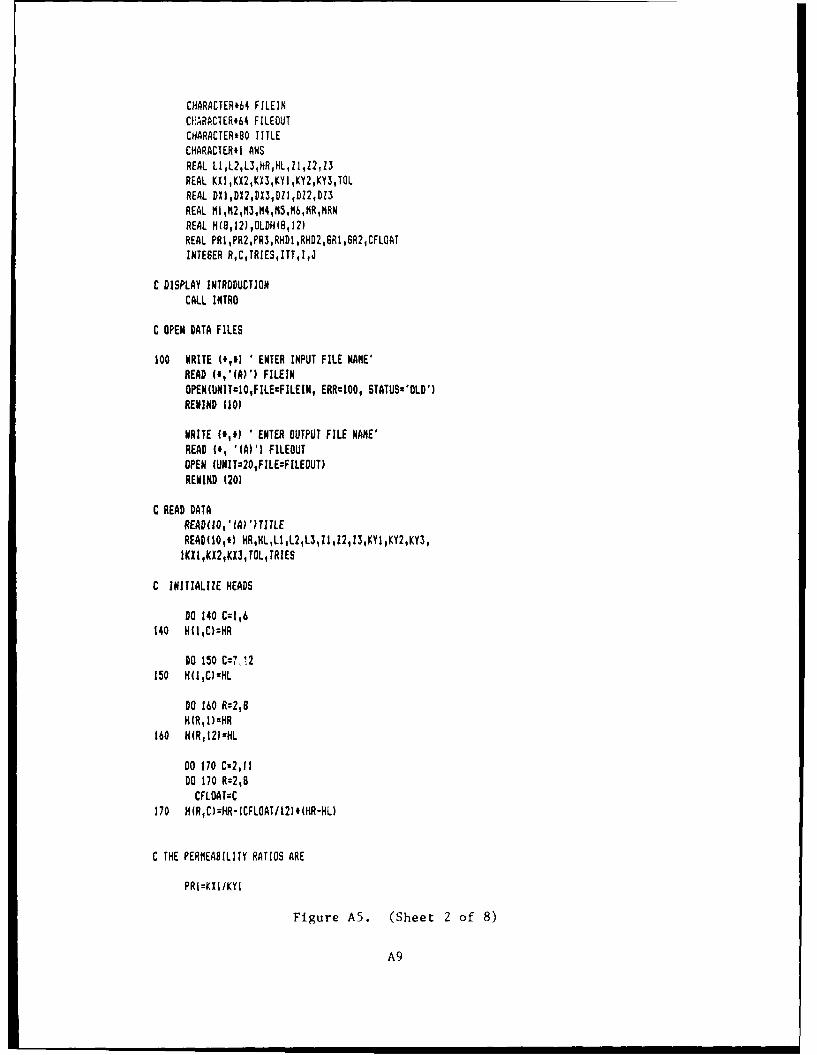
CHARACTER*64 FILEINCEARACTER.64 FILEOUTCHARACTER&S0 TITLECHARACIERII ANSREAL LI,L2,L3,HR,HLZI,22,l3REAL KXI,KX2,K.I3,KYI,KY2,KY3,TOLREAL DXI,DX2,DX3,Dl1,DZ2,DZ3REAL M11N21l13,t4,M5,t16,MR,?1RNREAL H(8,12),IJLDHI8,12)REAL PRIPR2,PR3,RHDI,RHD2,6R1,6R2,CFLOATINTEGER RC,TRIESITT1IJ
C DISPLAY INTRODUCTIONCALL INTRO
C OPEN DATA FILES
100 WRITE (*,l') ENTER INPUT FILE NAME'READ (#,'(A)') FILEINOPEN(UNITSIO,FILEzFILEIN, ERR41O0, STATUSxSOLD')REMIND (10)
WRITE (#I0') ENTER OUTPUJT FILE NME'READ 0', '(W) FILEOUTOPEN (UNIT=20,FILEzFILEOUT)REWIND (20)
C READ DATAREAD(1O,-lA? ?TlTLEREAD(10,4) HR,HLL1,L2,L3,11,Z2,13,KY1,KY2,KY3,IKXZ ,KX2,KX31 TOL,TIES
C INITIALIZE HEADS
DO 140 Cxl,6140 H(IqC):HR
DO 150 C=7,12150 H(1,C)=HL
DO 160 R=2,8HIR 11)=HR
160 H(R,12)41HL
DO 170 C=2,11DO 110 R=2,8CFLOAT=C
170 H(R,C)=HR-1CFLOAT/12)1(HR-HL)
C THE PERMIEABILITY RATIOS ARE
Figure A5. (Sheet 2 of 8)
A9
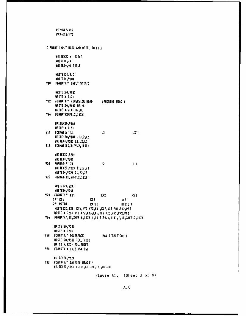
PR2=KX2/KY2PR3=KXSIKYS
C PRINT INPUT DATA AND WRITE TO FILE
WRITE(20,#) TITLEWRITE010.NRITE010. TITLE
WRITE (20,910)WRITE(',910)
910 FORMlAT(/' INPUT DATA')
WRITE (20,912)WRITE(4,912)
912 FORMAT(/ RIVERSIDE READ LANDSIDE HEAD')WRITE(20,914) HR,HLWRITE(0,914) HR,HL
914 FORtIATW2F9.2,I I ))
WRITE (20,916)WRITE(I,916)
916 FORHAT(I 11 12 L3')WRITE(20,918) L1,L2,L3WRITE14,910) 11,12,L3
918 FORMATUI1,3(F9.2,1IXI)
WRITE (20,920)WRITE(#,920)
920 FORMAT( I i2DWRITE(20,9221 11,12,13WRITE(',922) 11,12,13
922 FORMAT(11,3(F.2,11X)
WRITE (20,924)WRITE (*,924)
924 FORMAT(/ KYI KY2 KY3'11' KXI KX2 X21' RATIO RATIO RATIO')WRITE120,926) KYI,KY2,KYS,KXI,KX2,KX3,PRI,PR2,PR3WRITE(#,926) KYI,KY2,KYS,KXI,KX2,KX3,PRI,PR2,PR3
926 FORHAT(I,11,3(F.6,1t[),I,IX,3(F9.6,111),/,11,3(F9.2,1IX))
MRITE(20, 928)WRITE (#,928)
928 FORMAT(/' TOLERANCE MAX ITERATIONS')WRITE(20,9301 TOL,TRIESWRITEIe,930) TOL,TRIES
930 FORMAT(II,F9.5,ISX,I5)
WRITE (20, 932 I932 FORHATI/' iNITIAL HEADS')
WRITEI20,7341 (IN)R,C),C=1,12),R:1,B)
Figure A5. (Sheet 3 of 8)
AIO
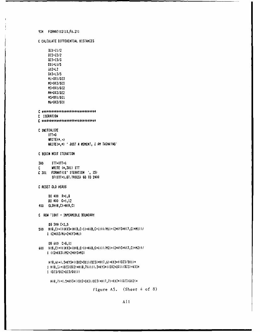
934 FORMAT(12h1X,F6.2))
C CALCULATE DIFFERENTIAL DISTANCES
D0I=112D122:2/2D13=213DX11:1/5DX2=L2DX3=13/5
M2:-DX3/DZ3
M4=DX3IDZ2M5=DXI/DZIM6zDX3IDlI
C *411,*l14*04f1**
C ITERATIONC eI.E.H114IIII*l
C INITIALIZEITTZOWRITE(#'d)WRITE(4,f) ' JUST A MOMENT, I AN THINKING'
C BEGIN NEXT ITERATION
300 ITT=ITT+1C WRITE (0,301) ITTC 301 FORMAT(IX' ITERATION ', 15)
IF(ITT+1.GT.TRIES) 6010O2400
C RESET OLD HEADS
DO 400 R=I,8DO 400 Cz:1,12
400 OLDH(R,C)=HIR,C)
C RaM 718HT - IMPERMEBLE BOUNDARY
0O 500 C=2,5500 H(8,C)3(((KX3t(H(8,C1I)4H(BqC44)))/I11)+(2tKY3'H(7,C)MIl)I/
I (2*KX3/MI42fKY3#hI)
00 600 C=8,11600 H(B,C):(((KX3.(H(B,C-1)+H(8,C+I)/M2)+I2IKY3#H7,C)*12))/
I ((24KX31/fl2+2fKY3#l2)
H!B,6)=(.5,KY3#((DX2+DXI)/DZ3)4H(7,6)+K13#((D23/DX I)'I H(8,5it(D23/DX2?.H(8,7)i )/(.5,KY3#( (DX2*DXI)/D23)+KX3.
I (DZ3/DX2+D23/DXI))
H18,7):(.5*KY3,(fO12+DX3)/D23),Hl7,7)+KX i3(Dl3/DX2)*
Figure A5. (Sheet 4 of 8)
All
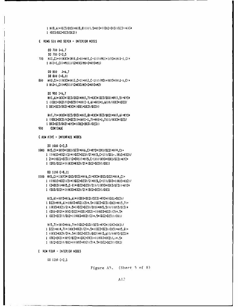
I (DIS/D12+DZ3IDXS))
C ROWS SIX AND SEVEN - INTERIOR NODES
001700 1=6,7DO 700 C=2,5
700 H(IC)z(((KX3*CH(I,C41)+H(I,C-1)))/Mi1)*1KY3.(H(I-IC)+
DO 800 J=6,7DO 800 C:8,11
800 H(J,C):(((KX3*(H(J,C+1),H(J,C-1)))/1121+(KY3.(H(J-1,C)41 H(J,1,C))*Ii2))I(2*KX3/l 2+2*KY3*M2)
DO 900 1=6,7
1 I)((DX1+D/(2DX2l)@(C1,).HX3(+1,6)))(H3(13/,K
I DXI.DZ3IDX2).KY3#((DX1+DX2)IDl3))
H(1,7)u(KX3#(Dl3/Il3)#H([1,)+KX3.(Dl31DX2)'H(1,6)+KY3*I ((DX2.DX3)/(24DZ3))4(H(I-1,7)+H(I1,17))1/(KXSe(Dl3/I D13+D13/DX2)+KY3#((DX2.DX3)/D131)
900 CONTINUE
C ROW FIVE - INTERFACE NODES
DO 1000 C=2,51000 H(5,C)z(KY3#(DXI/DZ3)'H(6,C)sKY2.(DXI/Dl2)#H(4,CI+
1 ((CKX3+KX2)/2)#((Dl2.DZ3)/2).H(5,C+I)I/DX1 'KX3+KX2)/I 2)'((012+DZ3)/I2'DD1i)IH(5,C-1) l/(KY3#(D11/D13)+KY2'I (DXIIDZ2)+(((KX3+KX2)l2)#(DZ2+DZ3))IDX1)
DO 1100 C=8,111100 H(5,C)=((KY34CDX3/Dl3),H(6,C),KY2*(DX3/Dl2lH(4,C)+
I (((KX3+KX2)I2)#((DZ2.DZ3)l2)'H(5,C+1))IDX34((KX3+KX2)lI (2#DX3))#H(5,C-l)e(D!24DZ3)I2))/I(KY3.(DX3/DZIe)KY2I (DX3IDZ2)+(((KX3+KX2)I2)*(Dl2+DZ3))/DI3I
H(5,6)z(KY3*H(6,6)4( (DXI+DX2)/DZ3)+KY2'( (D11+DX21/
I ((KX3+KX2I/2)#.5e((O2.D3)/DXI)H(5,5/((KY3/DZ3)#I (DXI+DX2)+IKY2/DZ2)#(DXI+DX2).(((KX3+KX2)/2I'.5#I (DZ2+D13))/DX2+(I(KXStKX2)12)#.5#(DZ2.D13))IDXI)
H(5,7)=(KY3*H(617)4I(DX2+DX3)/D13)4KY2i( (012+01311I D12)#H(4,7)$((KX3+KX2)/2)'.5*'(D2DZ3)/DX31eH(5,8)+I ((KX3.KI2)/2)'.5'((DZ2+DZ3)/012I'H(5,6)(/((KY3(DZ3)#1 (D12tDX3)+IKY2/D12)'1012+DX3)+( ((KI3+KX2)/i*.5'1 (D12+DZ3))/DX3+(((KX3+KX2)/2)#.5#(012.Dl3))/DX2)
C ROW FOUR - INTERIOR NODES
DO 1200 C=2,5
Figure A5. (Sheet 5 of 8)
A12
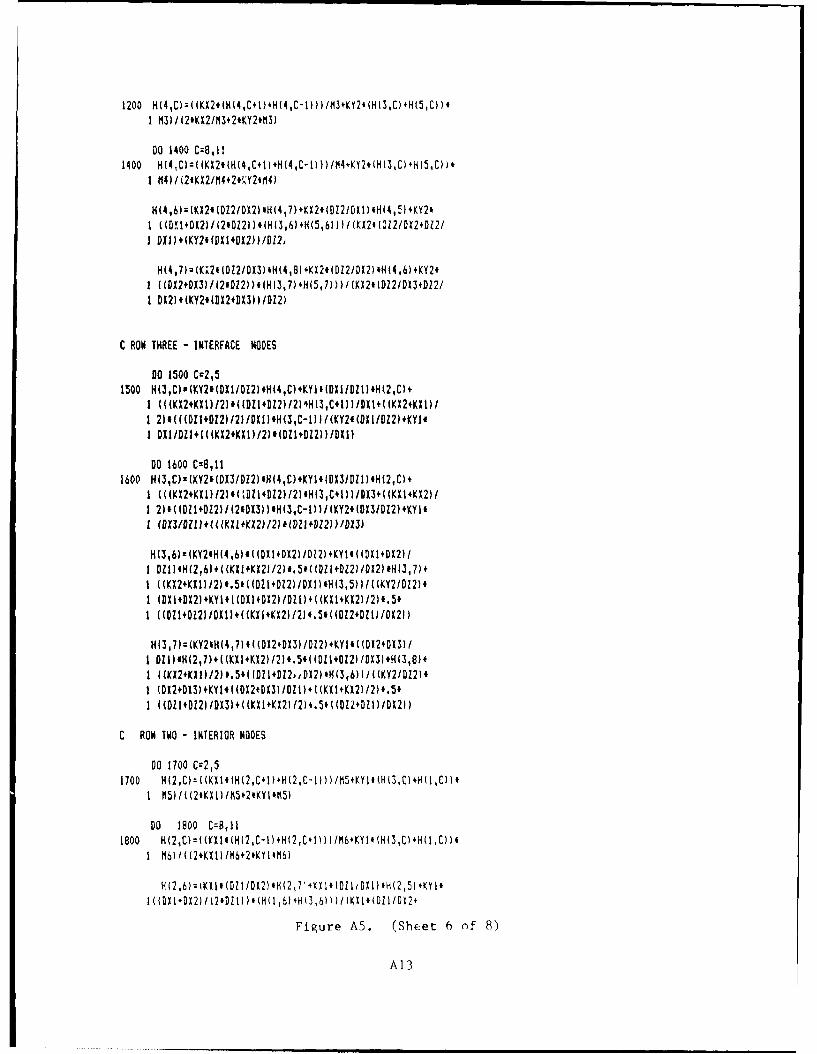
I I3)/(2*KI2IM3+2tKY2t13)
DO 1400 C=8l111400 H(4,C:(IK2(H(4,C+)+(4,C-1)))/M4+KY2t(H(3,C) HI5,C) )*
I l4) /i2IKX2/fl4+2§'AY2lM41
H(4,6):(KX2*(D22/DX2)#H(4,7)+K02*(D22/DXI)IN(4,5(4KY2*1 ((DX1+DX2)/(24Dl2I)t(H(3,6)+H(5,61fl/(KX?4(012/DX2+Dl2/I DXI)+(KY2* (DXI +DX2) I1D12i
H(4,7):(K 2#lDl2/DX3).H(4,8) *KX2IIDL2/DX2) 'H(4,6)+KY2#1 IIDX2tDX3)/(2.D12))flHI3,7).H(5,7))1/ (KX2#(D2IDX3+D2II D12)+CKY2'(DX2+DX3))/DZ2)
C ROW THREE - INTERFACE NODES
0O 1500 Cc2,51500 H(3,C)s(KY2*(DX1/Dl2l.H(4,C)4KYlI(DXIDZI).H(2,C)+
1 (((KX24KXI)I2)#((DZ1+Dl?)/2l H(3,C+1) )IDXI+((KX2*KXI)/
I DXIIDZI.(((KX2+KXI)/2)#(DZI+DZ2)IDXI)
DO 1600 Cze,111600 H(5,C)z(KY2I(DX3/D22)'H(4,C)+KY14(DX3iDlI)*H(21C)+
I (((KX2+KXI)/2)#( .DZ14DZ2)l2).H(I,C41))IDX34((KXI+KX2)I1 2)#((DZI+D22)I(2*013))#H(3,C-1))I(KY2#(DX3/D22)+KYI'I(DX3/DZU.+(UIkX1KX2/??'ID1fDZ2))/DJ)
H13,6):(KY2IH(416)#4UDXI+DX2)/012)+KYti( (DXI*DX2)II DII'fH(2,6)+((Z11.2)/2)f..#((DlI+Dl2?/DX2HLN3 17)+1 ((KX2+KXI1)2)#.5#((DlI4Dl2)/DX1)'H(3,5))/((KY7IDZ2)#I (DXI+DX2)+KYII( (DX1+DX2) /DhI)+((KX14KX2)/2)#.5*
H(3,7)=(KY2*H(4,7)*1(0(12+D13)/DZ2)+KYII( CD12+DX3)/
1 ((KX2+KXI)/2)'.5#((DZl+DZ2, 1DX2)#H(3,6flI((KY2ID2V1 (DX2+DI3)+KY14)(DX2+DX3lIDZ1)+((KXltKI2)/2)#.5#1 ((DZ1+DZ2)/DX3)+((KXI+KX21/2)'.5*((DZ2+DZI)1DX2()
C ROW TWO - INTERIOR NODES
DO 1700 C=2,51700 H(2,C):((KX1iIH(2,C+I+H(2,C-l)))/MJ*KYII(H(3,C)4H(l,C)lt
I M5)/((2*KXI)/M5+2#KYI*m5)
DO 1800 C=8,1l1800 H(2,C):((KXI4(H(2,C-l)+H(2,C#1fl)/Mb.KYlt(H(3,C)+H(14C))&
I Mb)/((2.KXI)/M6+2tKYI'M6)
Figure A5. (Sheet 6 of 8)
A13
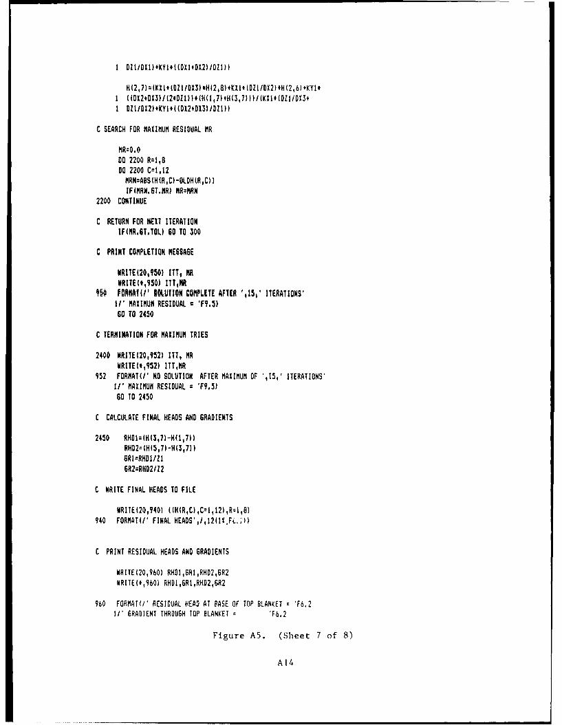
I DZ1/DXI)+KYI#I(OXI+DX2)/DZI))
H(2,7)=(KXi*(DZIIOX3)#H(2,8) KXI#(DZIIDX2)#H(2,6)+KYI#I ((OX2*OX3)I(2#DZI))#(H(1,7)+H(3,7)1)/(KXIe(ODII/XSI OZI/DX2)+KYI*((DX2+OX3)/DZI))
C SEARCH FOR MAXIMUM RESIDUAL MR
NR=OODO 2200 R=1,8DO 2200 C=1,12MRN=ABS(H(R,C)-OLDH(R,C))IF(M'RN. GT.MR) MR--MN
2200 CONTINUE
C RETURN FOR NEXT ITERATIONIF(MR.6T.TOL) 60 TO 300
C PRINT COMPLETION MESSAGE
NRITE(20,M5) ITT, MWR[TE(,930) ITT,NR
150 FORMAT(/' §OLUTION COMPLETE AFTER -,1 l' ITERATIONS'IV' MAXIMUM RESIDUAL c 1F9.5)
60 TO 2450
C TERMINATION FOR MlAXIMUM TRIES
2400 WRITE(20,952) 1TT, MRWRITE0t,952) ITT,MR
952 FORMAT(/' NO SOLUTION AFTER MAXIMUM OF ',15,' ITERATIONS'IV' MAXIMUM RESIDUAL = 7F9.5)60 TO 2450
C CALCULATE FINAL HEADS AND GRADIENTS
2450 RHOI=(H(Q,7)-H(I,T))RHD2=(H(5,7)-H(3,7))6RI=RHDI/Z!6R2=RHD21Z2
C WRITE FINAL HEADS TO FILE
WRITE(20,?401 ((H(R,C),C=1t12),Rz1,8)940 FORMAT(/' FINAL HEADS-,/,12(lX.F .;))
C PRINT RESIDUAL HEADS AND GRADIENTS
WRITE(20,960) RHDI,GRI,RHD2,GR2WRITE(0,90) RHDi,6RI,RHD2,GR2
960 FORMAT(/' RESIDUAL READ AT BASE OF TOP BLANKET 7 '6.2I1/ GRADIENT THROUGH TOP BLANKET = 'F6.2
Figure A5. (Sheet 7 of 8)
A 14
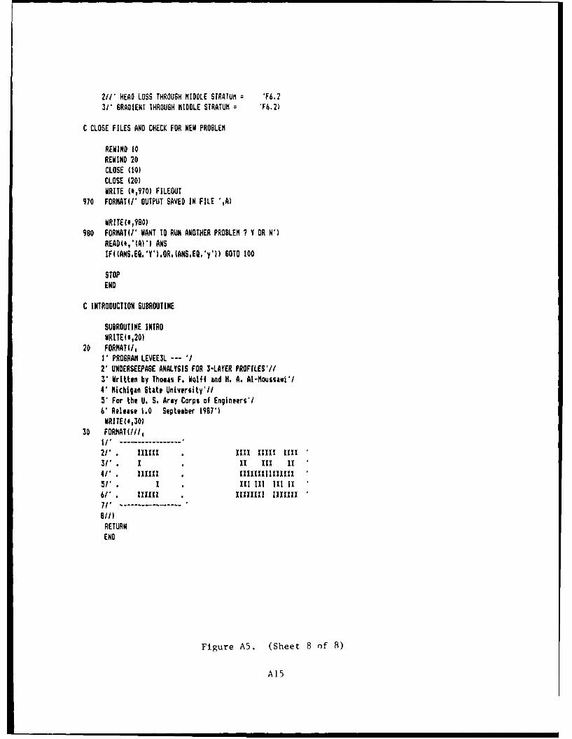
2//' HEAD LOSS THROUGH MIDDLE STRATUM 'F6.2
31' GRADIENT THROUGH MIDDLE STRATUM 'F6.2)
C CLOSE FILES AND CHECK FOR NEW PROBLEM
REWIND 10REWIND 20CLOSE (10)CLOSE (20)WRITE (,970) FILEOUT
970 FORMAT(/' OUTPUT SAVED IN FILE ',A)
WRITE(0,980)980 FORMAT(' WANT TO RUN ANOTHER PROBLEM ? Y OR N')
READ(*,'(A)'1 ANSIF((ANS.Eg.'Y').OR(ANS.EO.'y')) 60TO 100
STOPEND
C INTRODUCTION SUBROUTINE
SUBROUTINE INTROWRITE4i,20)
20 FORMAT(I,I' PROGRAM LEVEE3L -- '/2' UNOERSEEPA6E ANALYSIS FOR 3-LAYER PROFILES'//
3' Written by Thomas F. Wolff and H. A. Al-Moussawi'/4' Michigan State University'l5' For the U. S. Army Corps of Engineers'/6' Release 1.0 September 1987')WRITE0(,30)
30 FORMAT(//I,1/' --------2/1' IXXXxI . XXXX XXXx xxXI3/'• I . XX xxX IX41' , lXXI . XXIXXXXXXXIXX
5/' . I 1 I 1 lIX I IX6/ . xxxIIIxx XXXXXXI I11111171'
RETURNEND
Figure A5. (Sheet 8 of 8)
A15
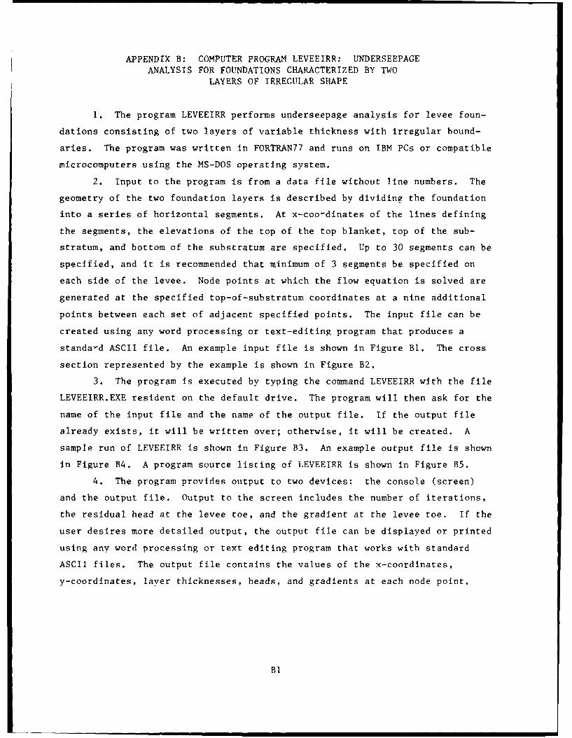
APPENDIX B: COMPUTER PROGRAM LEVEEIRR: UNDERSEEPAGE
ANALYSIS FOR FOUNDATIONS CHARACTERIZED BY TWO
LAYERS OF IRREGULAR SHAPE
1. The program LEVEEIRR performs underseepage analysis for levee foun-
dations consisting of two layers of variable thickness with irregular bound-
aries. The program was written in FORTRAN77 and runs on IBM PCs or compatible
microcomputers using the MS-DOS operating system.
2. Input to the program is from a data file without line numbers. The
geometry of the two foundation layers is described by dividing the foundation
into a series of horizontal segments. At x-coo-dinates of the lines defining
the segments, the elevations of the top of the top blanket, top of the sub-
stratum, and bottom of the substratum are specified. Up to 30 segments can be
specified, and it is recommended that minimum of 3 segments be specified on
each side of the levee. Node points at which the flow equation is solved are
generated at the specified top-of-substratum coordinates at a nine additional
points between each set of adjacent specified points. The input file can be
created using any word processing or text-editing program that produces a
standa'd ASCII file. An example input file is shown in Figure BI. The cross
section represented by the example is shown in Figure B2.
3. The program is executed by typing the command LEVEEIRR with the file
LEVEEIRR.EXE resident on the default drive. The program will then ask for the
name of the input file and the name of the output file. If the output file
already exists, it will be written over; otherwise, it will be created. A
sample run of LEVEEIRR is shown in Figure B3. An example output file is shown
in Figure B4. A program source liscing of LEVEEIRR is shown in Figure B5.
4. The program provides output to two devices: the console (screen)
and the output file. Output to the screen includes the number of iterations,
the residual head at the levee toe, and the gradient at the levee toe. If the
user desires more detailed output, the output file can be displayed or printed
using any word processing or text editing program that works with standard
ASCII files. The output file contains the values of the x-coordinates,
y-coordinates, laver thicknesses, heads, and gradients at each node point.
BI
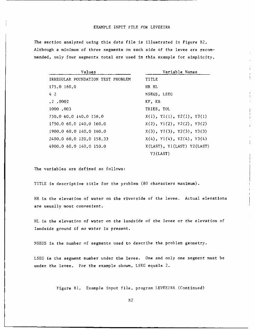
EXAMPLE INPUT FILE FOR LEVEEIRR
The section analyzed using this data file is illustrated in Figure B2.
Although a minimum of three segments on each side of the levee are recom-
mended, only four segments total are used in this example for simplicity.
Values Variable Names
IRREGULAR FOUNDATION TEST PROBLEM TITLE
175.0 160.0 HR HL
4 2 NSEGS, LSEG
.2 .0002 KF, KB
1000 .003 TRIES, TOL
750.0 60.0 140.0 158.0 X(1), Y1(1), Y2(1), Y3(1)
1750.0 60.0 140.0 160.0 X(2), YI(2), Y2(2), Y3(2)
1900.0 60.0 140.0 160.0 X(3), Y1(3), Y2(3), Y3(3)
2400.0 60.0 120.0 158.33 X(4), Y1(4), Y2(4), Y3(4)
4900.0 60.0 140.0 150.0 X(LAST), YI(LAST) Y2(LAST)
Y3(LAST)
The variables are defined as follows:
TITLE is descriptive title for the problem (80 characters maximum).
HR is the elevation of water on the riverside of the levee. Actual elevations
are usually most convenient.
HL is the elevation of water on the landside of the levee or the elevation of
landside ground if no water is present.
NSEGS is the number of segments used to describe the problem geometry.
LSEG is the segment number under the levee. One and only one segment must be
under the levee. For the example shown, LSEG equals 2.
Figure BI. Example input file, program LEVEEIRR (Continued)
B2

KF is the horizontal permeability of the suhstratum, in feet per minute or
other consistent units.
KB is the vertical permeability of the top blanket, in feet per minute or
other consistent units.
TRIES is the maximum number of iterations that the program will be allowed to
make. It is provided to stop the program in the event of non-converging solu-
tions. Generally the program should terminate because TOL is reached before
TRIES. A value of 500 is suggested.
TOL is the maximum tolerance, or maximum difference in head at any node
between successive iterations. The iteration process will stop when the maxi-
mum residual is smaller than TOL. A value of 0.001 is suggested.
X(1), YI(1), Y2(1), Y3(l) are the x-coordinate, the y-coordinate of the base
of the substratum, the y-coordinate of the base of the top blanket, and the
y-coordinate of the ground surface, respectively, at the riverside of the
first segment. This line is repeated for the riverside of each segment.
X(LAST), Yl(LAST), Y2(LAST), Y3(LAST) are the x-coordinate, the y-coordinate
of the base of the substratum, the y-coordinate of the base of the top
blanket, and the y-coordinate of the ground surface, respectively, at the land
side of the last segment.
Figure BI. (Concluded)
B3
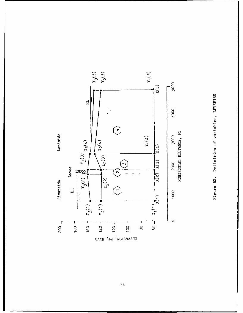
c~; N0
0-0
4-4
6Y C
0 EA 4w-4 -0 4)
CD C) ~ 0> 4 -41
4)-
0~c -ct1N
L1~? _ I C)0 0 '-I
H CI0
0 .1 c K
QIADN 'JA 'NOILVAaTI
B4
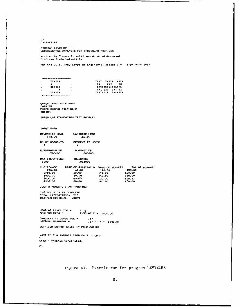
C>C>LEVEEIRR
PROGRAM LEVEEIRRUNOERSEEPAGE ANALYSIS FOR IRREGULAR PROFILES
Written by Thomas F. Wolff and H. A. AI-MoussawMichigan State University
For the U. S. Army Corps of Engineers Release 1.0 September 1987
XXXXXX XXXX XXXXX XXXXX XX XXX XXXXXXXX XXXXXXXIIXXXXXX
X XX1 IX! IXI IXXXXXXX XXXXXXXI IXXXXXX
ENTER INPUT FILE NAMEDATAIRRENTER OUTPUT FILE NAMEOUTIRR
IRREGULAR FOUNDATION TEST PROBLEM
INPUT DATA
RIVERSIDE HEAD LANDSIDE HEAD175.00 160.00
NO OF SEGMENTS SEGMENT AT LEVEE4 2
SUBSTRATUM KF BLANKET KB.200000 .000200
MAX ITERATIONS TOLERANCE1000 .003000
X DISTANCE BASE OF SUBSTRATUM BASE OF BLANKET TOP OF BLANKET750.00 60.00 140.00 158.00
1750.00 60.00 140.00 160.001900.00 60.00 140.00 160.002400.00 60.00 120.00 158.334900.00 60.00 140.00 150.00
JUST A MOMENT, I AM THINKING
THE SOLUTION IS COMPLETETOTAL ITTERATIONS- 298MAXIMUM RESIDUAL- .0030
HEAD AT LEVEE TOE - 7.38
MAXIMUM HEAD - 7.36 AT X - 1900.00
GRADIENT AT LEVEE TOE - .37MAXIMUM GRADIENT - .37 AT X - 1900.00
DETAILED OUTPUT SAVED IN FILE OUTIRR
WANT TO RUN ANOTHER PROBLEM 7 Y OR NN
Stop - Program terminated.
C>
Figure B3. Example run for program LEVEEIRR
B5
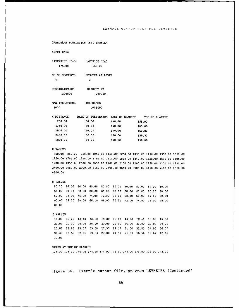
EXAMPLE OUTPUT FILE FOR LEVEEIRR
IRREGULAR FOUNDATION TEST PROBLEM
INPUT DATA
RIVERSIDE HEAD LANDSIDE HEAD
175.00 160.00
NO OF SEGMENTS SEGMENT AT LEVEE
4 2
SUBSTRATUM KF BLANKET KB
.200000 .000200
MAX ITERATIONS TOLERANCE
1000 .003000
X DISTANCE BASE OF SUBSTRATUM BASE OF BLANKET TOP OF BLANKET
750.00 60.00 140.00 158.00
1750.00 60.00 140.00 160.00
1900.00 60.00 140.00 160.00
2400.00 60.00 120.00 158.33
4900.00 60.00 140.00 150.00
X VALUES
750.00 850.00 950.00 1050.00 1150.00 1250.00 1350.00 1450.00 1550.00 1650.00
1750.00 1765.00 1780.00 1795.00 1810.00 1825.00 1840.00 1855.00 1870.00 1885.00
1900.00 1950.00 2000.00 2050.00 2100.00 2150.00 2200.00 2250.00 2300.00 2350.00
2400.00 2650.00 2900.00 3150.00 3400.00 3650.00 3900.00 4150.00 4400.00 4650.00
4900.00
D VALUES
80.00 80.00 80.00 80.00 80.00 80.00 80.00 80.00 80.00 80.00
80.00 80.00 80.00 80.00 80.00 80.00 80.00 80.00 80.00 80.00
80.00 78.00 76.00 74.00 72.00 70.00 68.00 66.00 64.00 62.00
60.00 62.00 64.00 66.00 68.00 70.00 72.00 74.00 76.00 78.00
80.00
Z VALUES
18.00 18.20 18.40 18.60 18.80 19.00 19.20 19.40 19.60 19.80
20.00 20.00 20.00 20.00 20.00 20.00 20.00 20.00 20.00 20.00
20.00 21.83 23.67 25.50 27.33 29.17 31.00 32.83 34.66 36.50
38.33 35.50 32.66 29.83 27.00 24.17 21.33 18.50 15.67 12.83
10.00
HEADS AT TOP OF BLANKET
175.00 175.00 175.00 175.00 175.00 175.00 175.00 175.00 175.00 175.00
Figure B4. Example output file, program LEVEEIRR (Continued)
B6
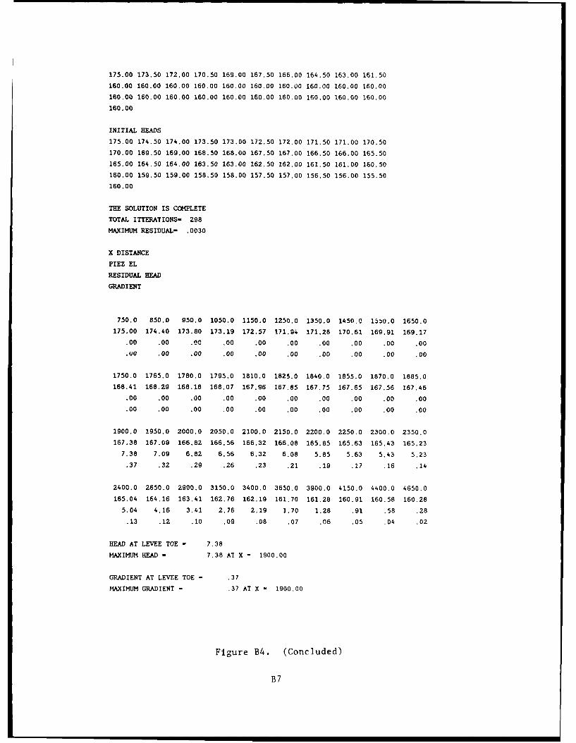
175.00 173.50 172.00 170.50 169.00 167.50 166.00 164.50 163.00 161.50
160.00 160.00 160.00 160.00 160.00 160.00 160.00 160.00 160.00 160.00
160.00 160.00 160.00 160.00 160.00 160.00 160.00 160.00 160.00 160.00
160.00
INITIAL HEADS
175.00 174.50 174.00 173.50 173.00 172.50 172,00 171.50 171.00 170.50
170.00 169.50 169.00 168.50 168.00 167.50 167.00 166.50 166.00 165.50
165.00 164.50 164.00 163.50 163.00 162.50 162.00 161.50 161.00 160.50
160.00 159.50 159.00 158.50 158.00 157.50 157.00 156.50 156.00 155.50
160.00
THE SOLUTION IS COMPLETE
TOTAL ITTERATIONS- 298
MAXIMUM RESIDUAL- .0030
X DISTANCE
PIEZ EL
RESIDUAL HEAD
GRADIENT
750.0 850.0 950.0 1050.0 1150.0 1250.0 1350.0 1450.0 15!0.0 1650.0
175.00 174.40 173.80 173.19 172.57 171.94 171.28 170.61 169.91 169.17
.00 .00 .00 .00 .00 .00 .00 .00 .00 .00
.00 .00 .00 .00 .00 .00 .00 .00 .00 .00
1750.0 1765.0 1780.0 1795.0 1810.0 1825.0 1840.0 1855.0 1870.0 1885.0
168.41 168.29 168.18 168.07 167.96 167.85 167.75 167.65 167.56 167.46
.00 .00 .00 .00 .00 .00 .00 .00 .00 .00
.00 .00 .00 .00 .00 .00 .00 .00 .00 .00
1900.0 1950.0 2000.0 2050.0 2100.0 2150.0 2200.0 2250.0 2300.0 2350.0
167.38 167.09 166.82 166.56 166.32 166.08 165.85 165.63 165.43 165.23
7.38 7.09 6.82 6.56 6.32 6.08 5.85 5.63 5.43 5.23
.37 .32 .29 .26 .23 .21 .19 .17 .16 .14
2400.0 2650.0 2900.0 3150.0 3400.0 3650.0 3900.0 4150.0 4400.0 4650.0
165.04 164.16 163.41 162.76 162.19 161.70 161.28 160.91 160.58 160.28
5.04 4,16 3.41 2.76 2.19 1.70 1.28 .91 .58 .28
.13 .12 .10 .09 .08 .07 .06 .05 .04 .02
HEAD AT LEVEE TOE - 7.38
MAXIMUM HEAD - 7.38 AT X - 1900.00
GRADIENT AT LEVEE TOE = .37
MAXIMUM GRADIENT - .37 AT X - 1900.00
Figure B4. (Concluded)
B7
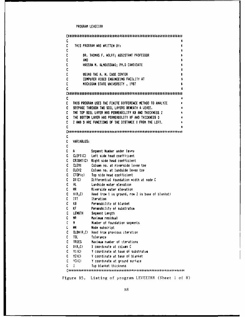
PROGRAM LEVEEIRR
CC THIS PROGRAM WAS WRITTEN BY: $C $C DR. THOMAS F. WOLFF; ASSISTANT PROFESSOR $C AND $C HASSAN M. ALMOUSSAWI; PH.D CANDIDATE $C $C USING THE A. H. CASE CENTER $C COMPUTER AIDED ENGINEEING FACILITY AT $C MICHIGAN STATE UNIVERSITY , 1987 $C $
CC THIS PROGRAM USES THE FINITE DIFFERENCE METHOD TO ANALYZE fC SEEPAGE THROUGH TWO SOIL LAYERS BENEATH A LEVEE. fC THE TOP SOIL LAYER HAS PERMEABILITY KB AND THICKNESS Z #
C THE BOTTOM LAYER HAS PERMEABILITY KF AND THICKNESS D #C Z AND D ARE FUNCTIONS OF THE DISTANCE X FROM THE LEFT.C *
CC VARIABLES:CC A Segment Number under leveeC CLEFT(C) Left side head coeffi:ientC CRIGHTIC) Right side head coefficientC CLEVI Column no. at riverside levee toeC CLEV2 Column no. at landside levee toeC CTOP(c) Top side head coefficientC DX(C) Differential foundation width at node CC HL Landside water elevationC HR Riverside water elevationC H(R,C) Head (row I is ground, row 2 is base of blanket)C ITT IterationC KB Permeability of blanketC KF Permeability of substratumC LENGTH Segment LengthC MR Maximum residualC N Number of foundation segments
NN Node subscriptC OLDH(RC) Head from previous iterationC TOL ToleranceC TRIES Maximum number of iterationsC X(RC) X coordinate at column CC YI(C) Y coordinate at base of substratumC Y2(C) Y coordinate at base of blanketC Y3(C) Y coordinate at ground surfaceC Z Top blanket thickness
Figure B5. Listing of program LEVEETRR (Sheet 1 of 8)
B8
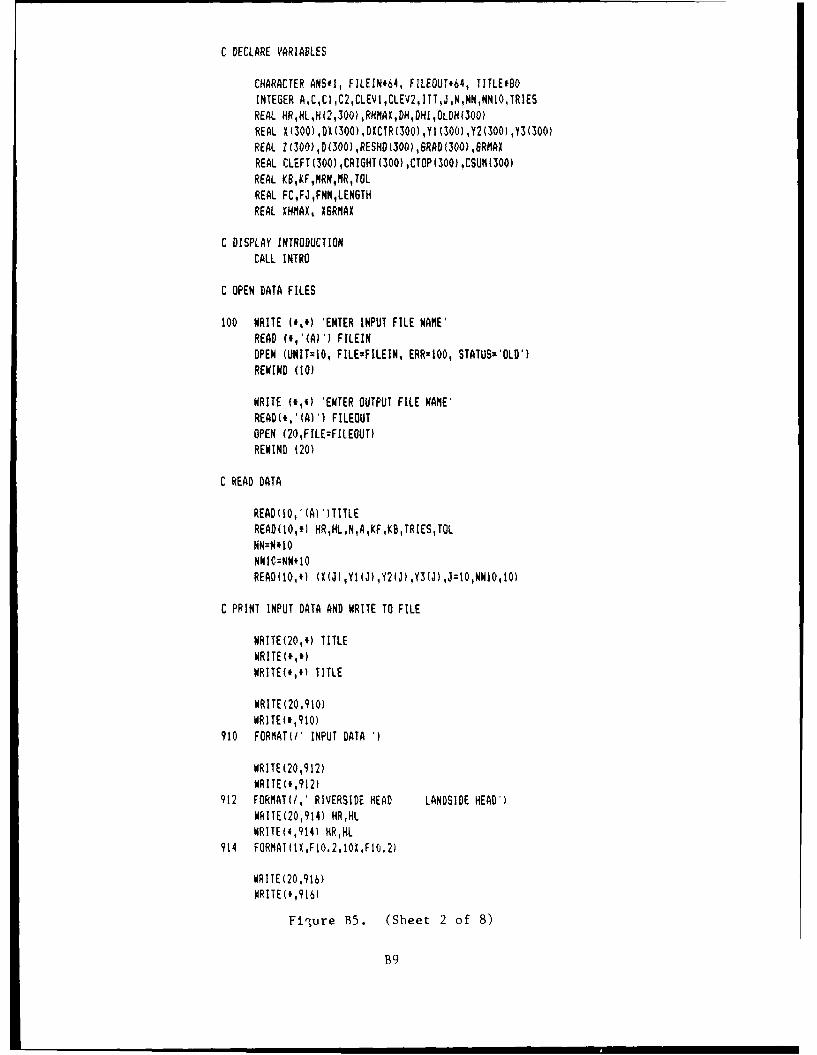
C DECLARE VARIABLES
CHARACTER ANS*I, FILE1NE64, FlLEOUT#64, TITLE*8OINTEGER AC,C1,C2,CLEV1,CLEV2,ITT,J,N,NN,NNIO,TRIESREAL HR,NLH(2,300),RHNAXDH,DHIOLDH(30O)REAL X(300),DX(300),DXCTR(300),YI(300),Y2(300),Y3(30i)REAL Z(300.),D(300),RESND(300),SRADi300L,SRMAXREAL CLEFT(300) ,CRIGHT(300) ,CTOP(300) ,CSUM(300)REAL IKB,KF,MRNMR,TOLREAL FC,FJ ,FNN,LENGTHREAL KHflAX, X6RMAX
C DISPLAY INTRODUCTIONCALL INTRO
C OPEN DATA FILES
100 WRITE C,*) 'ENTER INPUT FILE NAME'READ (#,'(A)') FILEINOPEN (UNIT=10, FILE=FILEIN, ERR=100, STATUS='OLD')REWIND (10)
WRITE (e,') 'ENTER OUTPUT FILE NAME'READ(#,'(A)-) FILEOUTOPEN (20,FILE:FILEOUT)REWIND (20)
C READ DATA
READ(10,'(A) ')TITLEREAD(10,*i HR,HL,N,A,KF,KB,TRIES,TOLNN:N*10NN1C=NN+10READ(10,') (X(J)YI(J),Y2(J),Y3(J),J=l0,WNIOqIO)
C PRINT INPUT DATA AND WRITE TO FILE
WRITE(20,*) TITLEWRITE(fq)WRITE(#,#) TITLE
WRITE(20,910)WRITE(',910)
910 FORMAT(/' INPUT DATA '
WRITE (20,912)WRITE C',912)
912 FORMAT(/,' RIVERSIDE HEAD LANDSIDE HEAD')WRITE(20,914) HR,HLWRITE(4,914) HR,HL
914 FORMATIlX,F10.2,l0X,Fl0.2)
WRITE(20,916)WRITE(#,9 16)
Fiiyure B5. (Sheet 2 of 8)
B9
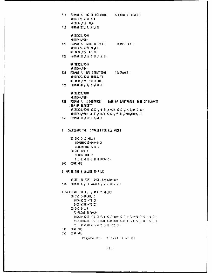
916 FORMIAT(/,' NO OF SESMENTS SE6MENT AT LEVEE')WRITE(20,918) NAWRITE(#,918) NA
918 FORMArtIX,1 3,17X,13)
WRITE (20 ,920)WRITE('4 920)
920 FORMAT(/,' SUBSTRATU .KF BLANKET KB')WRITE(20,922) KF,KBWRITE(I,922) KF,KB
922 FORMAT(IX,F12.6,8X,F12.6)
WRITE(20,924)WRITE0(,924)
924 FORMAT(/,' MAX ITERATIONS TOLERANCE')WRITE(20,926) TRIESTOLWRITE(#,92b) TRIESTOL
926 FORMAT(IX,15,15X,F1O.6)
WRITE (20,928)WRITE(*,928)
928 FORMAT(/,' X DISTANCE BASE OF SUBSTRATUM BASE OF BLANKETITOP OF BLANKET')WRITE(20,930) (X(J),YI(J),Y2)J),Y3(J),J:I0,NNIO,IO)
930 FORMAT)IX,4(FlO.2,6X))
C CALCULATE THE I VALUES FOR ALL NODES
DO 200 C=1O,NN,10LENGTHzX(C+10)-X(C)DX(C)zLENGTH/10.0
DO 200 J=1,9DX(C+J):DX(C)X(C+J)=X(C+J-1)+DX(C+J-1)
200 CONTINUE
C WRITE THE I VALUES TO FILE
WRITE (20,935) (X(C), C:I0,N4O)935 FORMAT (/,' X VALUES',/,IO(11F7.2))
C CALCULATE THE. D, 1, AND Y3 VALUESDO 350 C=IO,NN,10
D(C)zY2(C)-Yl(C)Z(C):-Y3(C)-Y2(C)
DO 340 J=1,9FJ=FLOAT)J)f 10.0
Z(C+J)=Y3(C)-Y2(C)+FJ#UIS)C4IO)-Y3(Cl-FJ(Y2(C)0)-Y2(C)Y3(C+J):V3(C)4FJ*(Y3)C+10)-Y3(C))
340 CONTINUE350 CONTINUE
Figure B5. (Sheet 3 of 8)
B 10C

D(NN1O)0Y2(NN1O)-104N1O)
Z (NNl0)=Y3(NNl0) -Y2(NNIO)
C WRITE THE D AND IVALUES TO FILE
WRITE(20,940)940 FORMAT(/,' D VALUES')
ORITE(?O,941) 010C, CzJ0,NN+10)941 FORMAT(IQ(1XF6.2))
WRITE (20 ,942)
942 FORMAT(/,' Z VALUES')WRITE(20,941) Q1(C), C=1O,NN,10)
C FIND THE COLUMNS UNDER THE LEVEE -- CLEVI TO CLEV2
CLEVI a A010CLEY2 c CLEVI 4 10
C CALCUALATE HEAL CHANGES AT LEVEE/BLANKET INTERFACE
IF(Y3(CLEV2).GT.HL) THENDHm:(HR-Y3(CLEV2) )/10.0
ELSEDH=(HR-HLU/10.0
END IF
C CALCULATE THE HEAD AT TOP OF BLANKET
DO 400 C=I0,NN1O
C RIVERSIDEIF(C.LE.CLEVI) THEN
H(1 .C):HR
C LEVEEELSEIF((C,6T.CLEVI).AND,(C.LT.CLEY2)) THENH(1,C)kH(1,C-I)-DH
C LANDS IDE - WATER ABOVE GROUNDELSEIF((C.6E.CLEV2).AND,(HL.GT.Y3(C)fl THEN
H)), C) :HL
C LANDSIDE - GROUND ABOVE WATERELSE
END! F
C LANDSIDE - HIGH GROUND ABOVE HRIFIIC.GE.CLEV2).AND,)H(1,C).6T.HR) THEN
END IF
40) CONTINUE
Figure B5. (Sheet 4 of 8)
BI I
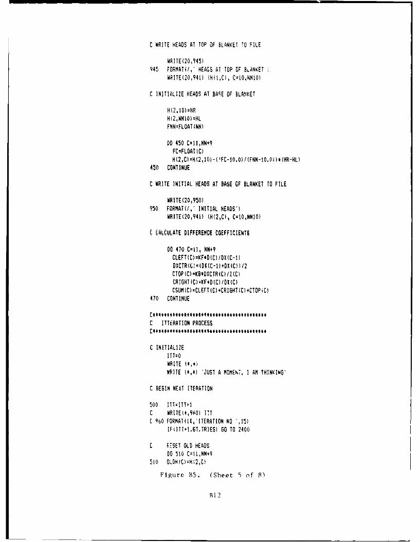
C WRITE HEADS AT TOP OF BLANKET TO FILE
WRITE(20,945)945 FORMAT(/,' HEADS AT TOP OF BtANKET
WRITE(20,941) (H!I,C), C=10,010O)
C INITIALIZE HEADS AT BAE OF BLANKET
H(2.10)=HRH(2,NNIO)=HL
FNN=FLOAT(NN)
DO 450 CcII,NN+9FC=FLOAT(C)H(2,C):H(2,10)-( FC-I0.0)t(FNN-10.0))*(HR-HL)
450 CONTINUE
C WRITE INITIAL HEADS AT BASE OF BLANKET TO FILE
WRITE(20,950)950 FORMAT(/,' INITIAL HEADS-)
WRITE(20,941) (H(2,C), C=t0,NNIO)
C ALCULATE DIFFERENCE COEFFICIENTS
DO 470 C:1I, NN+9CLEFT(C):KF*D(C)/DX(C-I)DXCTR(C)=(DX(C-I)+DX(C))/2CTOP(C)=KBDXCTRC)/Z(C)CRIGHT(C)=KF*D(C)/DX(C)CSUM(C)=CLEFT(C)+CRI6HT(C) CTOP(C)
470 CONTINUE
C ITTERATION PROCESS
C INITIALIZEITT=OWRITE (t,t)WRITE (*,*) 'JUST A MOMENT, I AM THINKING'
C BE6IN NEXT ITERATION
500 ITT:ITT+1C WRITE(*,9AO) ITTC 960 FORMAT(IX,'ITERATION NO ',15)
IF(ITT+I.GT.TRIES) GO TO 2400
C FSET OLD HEADSDO 510 Czl1,NN+9
510 OLDH(C):H(2,C)
Figure B5. (Sheet 5 of 8)
BI 2
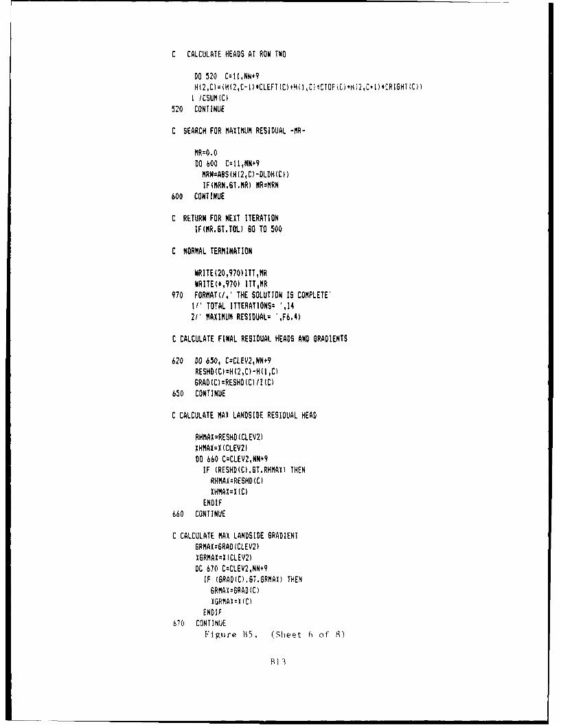
C CALCULATE HEADS AT ROW TWO
DO 520 C=11,NN49H(2,C):(H(2,C-l)*CLEFT(C)+H(l,C*CTOhiC)4H(2,C+I)ICRIGHT()CfI /CSUMIC)
520 CONTINUE
C SEARCH FOR MAXIMUM RESIDUAL -MR-
MR=0.QDO 600 C:11,NN+9MRN=ABS(H(2,C)-DLDH(C))IF(NRN.GT.MR) MRzMRN
600 CONTINUE
C RETURN FOR NEXT ITERATIONIF(MR.6T.TOL) 60 TO 500
C NORMAL TERMINATION
WRITE(20,970) ITTMRNRITE(.,970) ITT,MR
970 FORMAT(/,' THE SOLUTION IS COMPLETE'IV TOTAL ITTERATIONS: ',142/' MAXIMUM RESIDUAL= ',F6,4)
C CALCULATE FINAL RESIDUAL HEADS AND GRADIENTS
620 DO 650, C=CLEV2,NN#9RESHD(C)=H(2,C)-H(l ,C)6RAD(C)=RESHD(C) /Z(C)
650 CONTINUE
C CALCULATE MAX LANOSIDE RESIDUAL HEAD
RHtiAXzRESHD (CLEV2)XHMAX=X(CLEV2)00 660 C=CLEY2,NN49IF (RESHD(C).GT.RHMAX) THEN
RHMAX:-RESHD(C)XHMAIX X(C)
ENDIF660 CONTINUE
C CALCULATE MAX LANDSIDE GRADIENT6RMAXzGRAD CLEV2)XGRMAI:I (CLEV2)DO 670 C=CLEV2,NN+9IF (6RADIC).ST.GRMAX) THENGRMAX:GRAD(C)XGRMAI (C)
ENDIF670 CONTINUE
Figure B5. (Sheet 6~ of 8)
B]
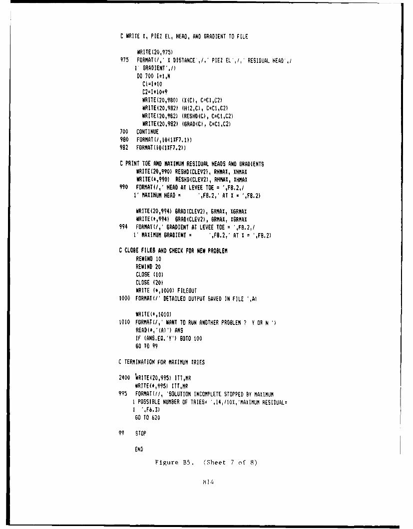
C WRITE X, PIEZ EL, HEAD, AND GRADIENT TO FILE
WRITE(20,975)975 FORMAT(/,' X DISTANCE',/,' PIEZ EL,!, RESIDUAL HEAD',/
I- GRADIENT',/DO 700 IzI,N
CI:I*OC2=I10+9WRITE(20,980) (X(C), C=CI,C2)WRITE(20,982) (H(2,C), C=CIC2)WRITE(20,982) (RESHD(C), C=CI,C2)WRITE(20,982) (GRAD(C), C=CI,C2)
700 CONTINUE980 FORMAT(/,10(IXF7.I))982 FORMAT(10(1XF7.2))
C PRINT TOE AND MAXIMUM RESIDUAL HEADS AND GRADIENTSWRITE(20,990) RESHD(CLEV2), RHMAX, XHMAXWRITE(i,990) RESHD(CLEV2), RHMAX, [HMAX
990 FORMAT(/,' HEAD AT LEVEE TOE m ',FB,2,/I' MAXIMUM HEAD c ',F8.2,' AT X = ',F8.2)
WRITE(20,994) 6RAD(CLEV2), 6RMAX, X6RMAXWRITE(*,994) GRAD(CLEV2), 6RMAX, XGRMAX
994 FORMAT(/,' GRADIENT AT LEVEE TOE = ',FB.2,/1' MAXIMUM GRADIENT z ',F8.2,' AT X = ',F8.2)
C CLOSE FILES AND CHECK FOR NEW PROBLEMREWIND 10REWIND 20CLOSE (10)CLOSE (20)WRITE (*,1000) FILEOUT
1000 FORMAT(/' DETAILED OUTPUT SAVED IN FILE ',A)
WRITE(*,1010)1010 FORMAT(/,' WANT TO RUN ANOTHER PROBLEM ? Y OR N 'I
READ(*,'(A)') ANSIF (ANS.EQ.'Y') SOTO 10060 TO 99
C TERMINATION FOR MAXIMUM TRIES
2400 WRITE(20,995) ITT,MRWRITE(*,995) ITT,MR
995 FORMAT(//, 'SOLUTION INCOMPLETE STOPPED BY MAXIMUMI POSSIBLE NUMBER OF TRIES% ',I4,/IOX,'MAXIMUM RESIDUAL=I ',F6.3)60 TO 620
99 STOP
END
Figure B5. (Sheet 7 of 8)
B14
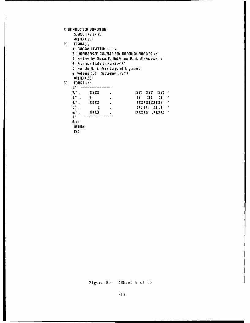
C INTRODUCTION SUBROUTINESUBROUTINE INTROORITE(0,20)
20 FORMAT(/,V PROGRAM LEVEEIRR '/2' UNDERSEEPAGE ANALYSIS FOR IRREGULAR PROFILES'//3' Written by Thomas F. Wolff and H. A. Al-Moussasi'/4' Michigan State University*//5' For the U. S. Army Corps of Engineers'6' Release 1.0 September 1987')WRITE( 30)
30 FORMAT(///,1/'21' . XXXXXX . XXXX XXXXX XXXX3/' . X . XX XXX XX
4/' . XXXIXX . XXXXXXXIIXXXXXX5/ 1X . XXI lXI IXI IX6/' . XXXXX , XXXXXXXI IXXXXX7/'
RETURNEND
Figure B5. (Sheet 8 of 8)
BI 5
APPENDIX C: COMPUTER PROGRAM LEVEECOR: UNDERSEEPAGE
ANALYSIS AT ANGLES OR "CORNERS" IN LEVEE ALIGNMENT
1. The program LEVEECOR performs underseepage analysis at bends or
corners in levee alignment. The program was written in FORTRAN77 and runs on
IBM PCs or compatible microcomputers using the MSD-DOS operating system.
2. Input to the program is from a 15 line data file without line
numbers. This file can be created using any word processing or text-editing
program that produces a standard ASCII file. An example input file is shuwn
in Figure C1. Program variables are defined in Figure C2.
3. The program is executed by typing the commvnd LEVEECOR with the file
LEVEECOR.EXE resident on the default drive. The program will then ask for the
name of the input file and the name of the output file. If the output file
already exists, it will be written over; otherwise, it will be created. A
sample run of LEVEECOP is shown in Figure C3. An example output file is shown
in Figure C4. A program source listing of LEVEECOR is shown in Figure C5.
4. The program provides output to two devices: the console (screen)
and the output file. Output to the screen includes the number of iterations,
the residual head at the levee toe, and the gradient at the levee toe. If the
user desires more detailed output, the output file can be displayed or printed
using any word processing or text-editing program that works with standard
ASCII files. The output file contains the approximate distances to adjacent
nodes, equation coefficients, and initial and final heads at each node point.
C1
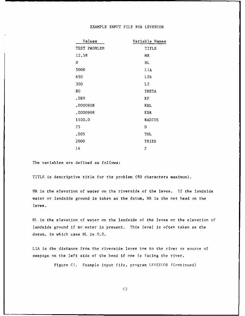
EXAMPLE INPUT FILE FOR LEVEECOR
Values Variable Names
TEST PROBLEM TITLE
12.58 HR
0 HL
5000 LIA
650 LIB
300 L2
80 THETA
.089 KF
.0000908 KBL
.0000908 KBR
1100.0 RADIUS
75 D
.005 TOL
2000 TRIES
14 Z
The variables are defined as follows:
TITLE is descriptive title for the problem (80 characters maximum).
HR is the elevation of water on the riverside of the levee. If the landside
water or landside ground is taken as the datum, HR is the net head on the
levee.
HL is the elevation of water on the landside of the levee or the elevation of
landside ground if no water is present. This level is often taken as the
datum, in which case HL is 0.0.
LIA is the distance from the riverside levee toe to the river or source of
seepage on the left side of the bend if one is facing the river.
Figure C1. Example input file, program LEVEECOR (Continued)
C2
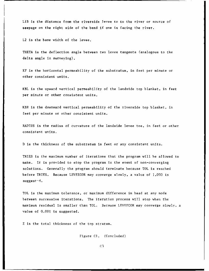
LIB is the distance from the riverside levee to to the river or source of
seepage on the right side of the bend if one is facing the river.
L2 is the base width of the levee.
THETA is the deflection angle between two levee tangents (analogous to the
delta angle in surveying).
KF is the horizontal permeability of the substratum, in feet per minute or
other consistent units.
KBL is the upward vertical permeability of the landside top blanket, in feet
per minute or other consistent units.
KBR is the downward vertical permeability of the riverside top blanket, in
feet per minute or other consistent units.
RADIUS is the radius of curvature of the landside levee toe, in feet or other
consistent units.
D is the thickness of the substratum in feet or any consistent units.
TRIES is the maximum number of iterations that the program will be allowed to
make. It is provided to stop the program in the event of non-converging
solutions. Generally the program should terminate because TOL is reached
before TRIES. Because LEVEECOR may converge slowly, a value of 1,000 is
suggest-d.
TOL is the maximum tolerance, or maximum difference in head at any node
between successive iterations. The iteration process will stop when the
maximum residual is smaller than TOL. Because LEVEECOR may converge slowly, a
value of 0.001 is suggested.
Z is the total thickness of the top stratum.
Figure C1. (Concluded)
C3
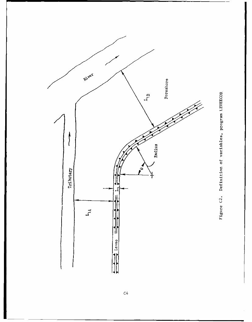
00
a))
0 0
r-'-
a
--4
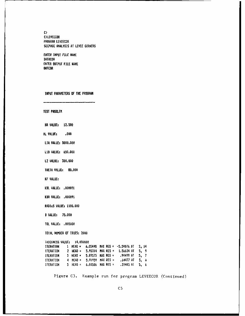
C>C)LEVEECOR
PROGRAM LEVEECORSEEPAGE ANALYSIS AT LEVEE CORNERS
ENTER INPUT FILE NAMEDATACORENTER OUTPUT FILE NAMEOUTCOR
INPUT PARAMETERS OF THE PROGRAM
TEST PROBLEM
HR VALUE: 12.580
HL VALUE: .000
LIA VALUE: 5000.000
LID VALUE: 650.000
L2 VALUE 300.000
THETA VALUE: 80.000
KF VALUE:
KBL VALUE: .000091
KBR VALUE: .000091
RADIuS VALUE 1100.000
D VALUE: 75.000
TOE VALUE: .005000
TOTAL NUMBER OF TRIES: 2000
iH0CKNESS VALUE: 14.000000ITERATION I HEAD 6.05448 MAX RES c -5.54076 AT 2, 14ITERATION 2 HEAD= 5.95314 MAX RES = 1.56634 AT 5, 9ITERATION 3 HEAD c 5.89575 MAX RES z .94499 AT 5, 7ITERATION 4 HEAD= 5.91939 MAX RES = .64477 AT 5, 6ITERATION 5 HEAO= 6.00586 MAX RES = .39485 AT 5, 6
Figure C3. Example run for program LEVEECOR (Continued)
C5
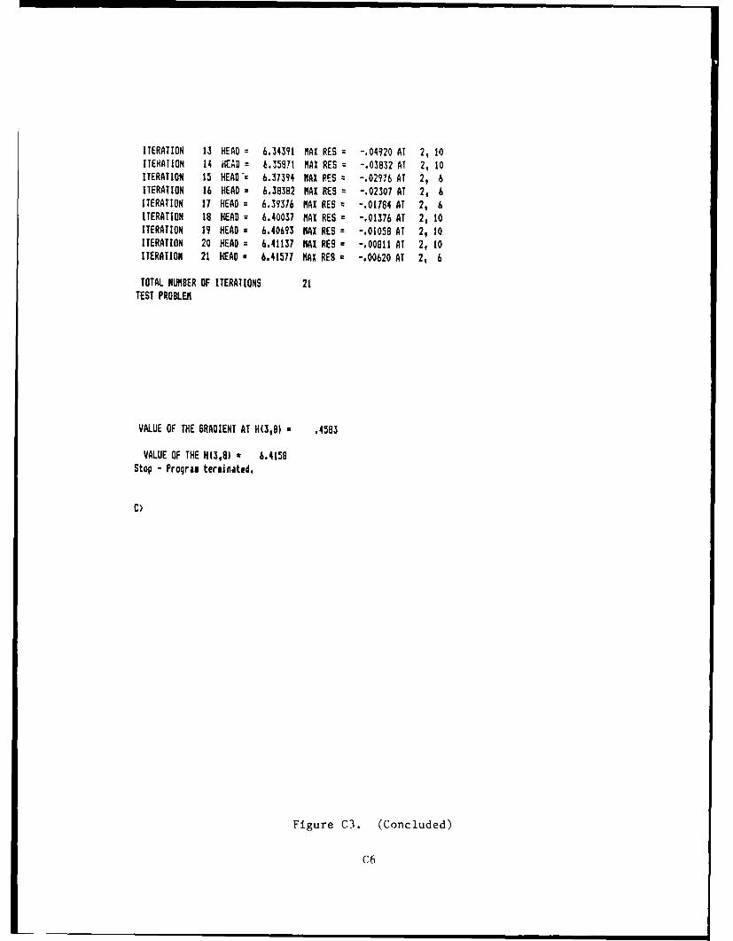
ITERATION 13 HEAD = 6.34391 MAX RES z -.04920 AT 2, 10ITEHATION 14 HEAD = 6.3587! MAX RES z -.03932 AT 2, 10ITERATION 15 HEAD-= 6.37394 MAX RES z -.02976 AT 2, 6ITERATION 16 HEAD z 6.38382 MAX RES = -.02307 AT 2, 6ITERATION 17 HEAD = 6.39376 MAX RES z -.01784 AT 2, 6ITERATION 18 HEAD = 6.40037 MAX RES z -.01376 AT 2, 10ITERATION 19 HEAD z 6.40693 MAX RES m -.01058 AT 2, 10ITERATION 20 HEAD = 6.41137 MAX RES -.00811 AT 2, 10ITERATION 21 HEAD a 6.41577 MAX RES a -.00620 AT 2, 6
TOTAL NUMBER OF ITERATIONS 21TEST PROBLEMI
VALUE OF THE 6RADIENT AT H(318) g .4583
VALUE OF THE H(3,8) • 6.4158Stop - Progras tersinated.
C)
Figure C3. (Concluded)
C6

EXAMPLE OUTPUT FILE FOR LEVEECOR
INPUT PARAMETERS OF THE PROGRAM
TEST PROBLEM
HR VALUE, 12.580HL VALUE .000LIA VALUEi 5000.000L! VALUE, 650.000L2 VALUE 300.000THETA VALUE, 80.000
KF VALUEs .089000KIL VALUE, ,000091KBR VALUEs .000091
RADIuS VALUEs 1100.000D VALUEt 75.000TOL VALUEs .005000TOTAL NUMBER OF TRIES, 2000THICKNESS VALUE, 14.000000INITIAL MATRIX.000 . .0000
.0000 .0000 .0000 .0000 .0000 .0000 .0000 .0000.0000 .0000 .0000 .0000 .0000 .0000 .00006.290 6.290 6.290 6. 290 6.290 6.290 6.2906.290 6.290 6.290 6.290 6.290 6.290 6.290
6.290 6.290 6.290 6.290 6.290 6.290 6.290 6.2906.290 6.290 6.290 6.290 6.290 6.290 6.290
6.290 6.290 6.290 6.290 6.290 6.290 6.290 6.2906.290 6.290 6.290 6.290 6.290 6.290 6,290
6.290 6.290 6.290 6,290 6.290 6.290 6.290 6.2906.290 6.290 6.290 6.290 6.290 6.290 6.290
12.58 12.58 12.58 12.58 12.58 12.58 12.58 12.5812.58 12.58 12.58 12.58 12.58 12.58 12.58
DXLEFT MATRIX.0000 1100. 1100. 1100. 1100. 1037. 20.00 20.00
20.00 20.00 1037. 1100. 1100. 1100. 1100..0000 1100. 1100. 1100. 1100. 1100. 20.00 20.00
20.00 20.00 1100. 1100. 1100. 1100. 1100.
.0000 1100. 1100. 1100. 1100. 1100. 384.0 384.0384.0 384.0 100. 1100. 1100. 1100. 1100.
.0000 1100. 1100. 1100. 1100. 1100. 488.7 488.7488.7 488.7 1100. 1100. 1100. 1100. 1100.
.0000 1100. 1100. 1100. 1100. 1100. 1172. 981.7791.9 602.1 1100. 1100. 1100. 1100. 1100.
.0000 1100. 1100. 1100. 1100. 1100. 1854. 1475.1095. 715.6 1100. 1100. 1100. 1100. 1100.
DRIGHT MATRIX
Figure C4. Example output file, program LEVEECOR
(Sheet I of 5)
C7
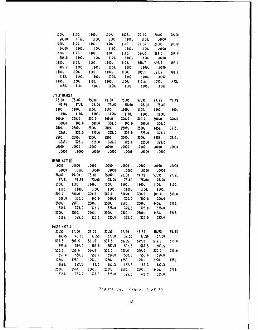
1100. 1100. 1100. 110J. 1037. 20.00 20.00 20.0020.00 1037. 1100. .100. 1100. 1100. .0000
1100. 1100. 1100. 1100. 1100. 20.00 20.00 20.0020.00 1100. 1100. 1100. 1100. 1100. .0000
1100. 1100. 1100. 1100. 1100. 384.0 384,0 384.0384.0 1100. 1100. 1100. 1100. 1100. .0000
1100. 1100. 1100. 1100. 1100. 488.7 488.7 48B.7488.7 1100. 1100. 1100. 1100. 1100. .0000
1100. 1100. 1100. 1100. 1100. 602.1 791.9 981.71172. 1100. 1100. 1100. 1100. 1100. .0000
1100. 1100. 1100. 1100. 2100. 715.6 1095. 1475.1854. 1100. 1100. 1100. 1100. 1100. .0000
DYTOP MATRIX75.00 75.00 75.00 75.00 75.00 97.91 97.91 97.91
97.91 97.91 75.00 75.00 75.00 75.00 75.001100. 1100. 1100. 1100. 1100. 1100. 1100. 1100.
1100. 1100. 1100. 1100. 1100. 1100. 1100.300.0 300.0 300.0 300.0 300.0 300.0 300.0 300.0
300.0 300.0 300.0 300.0 300.0 300.0 300.02500. 2500. 2500. 2500. 2500. 2500. 4456. 3913.
3369. 325.0 325.0 325.0 325.0 325.0 325.02500. 2500. 2500. 2500. 2500. 2500. 4456. 3913.
3369. 325.0 325.0 325.0 325.0 325.0 325.0.0000 .0000 .0000 .0000 .0000 .0000 .0000 .0000
.0000 .0000 .0000 .0000 .0000 .0000 .0000
DYBOT MATRIX
.0000 .0000 .0000 .0000 .0000 .0000 .0000 .0000.0000 .0000 .0000 .0000 .0000 .0000 .0000
75.00 75.00 75.00 75.00 75.00 97.91 W.91 97.9197.91 97.91 75.00 75.00 75.00 75.00 75.00
1100. 1100. 1100. 1100. 1100. 1100. 1100. 1100.1100. 1100. 1100. 1100. 1100. 1100. 1100.
300.0 300.0 300.0 300.0 300.0 300.0 300.0 300.0300.0 300.0 300.0 300.0 300.0 300.0 300.0
2500. 2500. 2500. 2500. 2500. 2500. 4456. 3913.3369. 325.0 325.0 325.0 325.0 325.0 325.0
2500. 2500. 2500. 2500. 2500. 2500. 4456. 3913.3369. 325.0 325.0 325.0 325.0 325.0 325.0
DYCTR MATRIX37.50 37.50 37.50 37.50 37.50 48.95 48.95 48.95
48.95 48.95 37.50 37.50 37.50 37.50 37.50587.5 587.5 587.5 587.5 587.5 599.0 599.0 599.0
599.0 599.0 587.5 587.5 587.5 587.5 587.5550.0 550.0 550.0 550.0 550.0 550.0 550.0 550.0
550.0 550.0 550.0 550.0 550.0 550.0 550.01250. 1250. 1250. 1250. 1250. 1250. 2228. 1956.
1684. 162.5 162.5 162.5 162.5 162.5 162.52500. 2500. 2500. 2500. 2500. 2500. 4456. 3913.
3369. 325.0 325.0 325.0 325.0 325.0 325.0
Figure C4. (Sheet 2 of 5)
C8
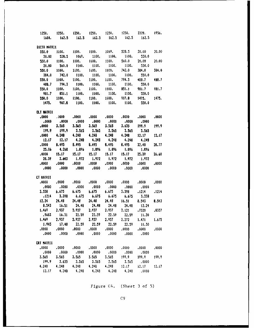
1250. 1250. 1250. 1250. 1250. 1250. 2228. 1956.1684. 162.5 162.5 162.5 162.5 162.5 162.5
DXCTR MATRIX550.0 1100. 1100. 1100. 109. 528.5 20.00 20.00
20.00 528.5 1069. 1100. 1100. 2100. 550.0550.0 1100. 1100. 1100. 1100. 560.0 20.00 20.00
20.00 560.0 1100. 1100. 1100. 1100. 550.0550.0 1100. 1100. 1100. 1100. 742.0 384.0 384.0
384.0 742.0 1100. 1100. 1100. 1100. 550.0550.0 1100. 1100. 1100. 1100. 794.3 488.7 486.7
488,7 794.3 1100. 1100. 1100. 1100. 550.0550.0 1100. 1100. 1100. 1100. 851.1 981.7 981.7
981.7 851.1 1100. 1100. 1100. 1100. 550.0550.0 1100. 1100. 1100. 1100. 907.8 1475. 1475.
1475. 907.9 1100. 1100. 1100. 1100. 550.0
CLT MATRIX.0000 .A000 .0000 .0000 .0000 .0000 .0000 .0000
.0000 .0000 .0000 .0000 .0000 .0000 .0000.0000 3.565 3.565 3.565 3.565 3.635 199.9 199,9
199.9 199.9 3.565 3.565 3.565 3.565 3.565.0000 4.248 4.248 4.248 4.248 4.248 12.17 12.17
12.17 12.17 4.248 4.248 4.240 4.248 4.248.0000 8.495 9.495 8.495 8,495 8.495 32.48 28.77
25.06 4.268 1.896 1.996 1.896 1.896 1.896.0000 15.17 15.17 15.17 15.17 15.17 25.39 26.6028.39 3.603 1.972 1.972 1.972 1,972 1.972
.0000 .0000 .0000 .0000 .0000 .0000 .0000 .0000.0000 .0000 .0000 .0000 .0000 .0000 .0000
CT MATRIX
.0000 .0000 .0000 .0000 .0000 .0000 .0000 .0000.0000 .0000 .0000 .0000 .0000 .0000 .0000
3.338 6.675 6.675 6.675 6.675 3.398 .1214 .1214.1214 3.398 6.675 6.675 6.675 6.675 3.336
12.24 24.48 24.48 24.48 24.48 16.51 8.543 8.5439.543 16.51 24.48 24.48 24.48 24.48 12.24
1.469 2.937 2.937 2.937 2.937 2.121 .7320 .8337.9683 16.31 22.59 22.59 22.59 22.59 11.30
1.469 2.937 2,937 2,937 2,937 2,272 1.471 1.6751.945 17.49 22.59 22.59 22.59 22.59 11.30
.0000 .0000 .0000 .0000 .0000 .0000 .0000 .0000.0000 .0000 .0000 .0000 .0000 .0000 .0000
CRT MATRIX.0000 .0000 .0000 .0000 .0000 .0000 .0000 .0000
.0000 .0000 .0000 .0000 .0000 .0000 .00003.565 3.565 3.565 3.565 3.565 199.9 199.9 199.9
199.9 3.635 3.565 3.565 3.565 3.565 .00004.248 4.248 4,248 4.248 4.248 12.17 12.17 12.17
12.17 4.248 4.248 4.248 4.248 4.248 .0000
Figure C4. (Sheet 3 of 5)
C9
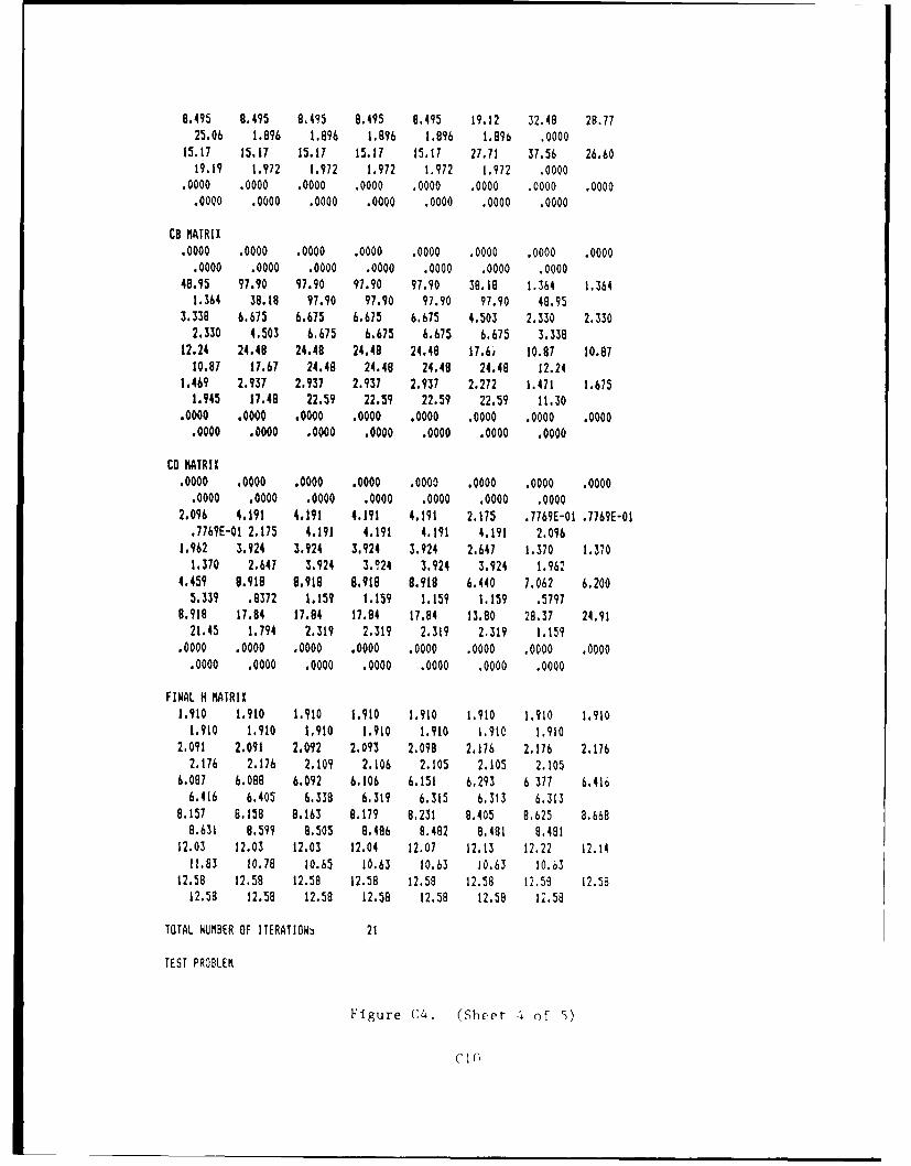
8.495 8.495 8.495 8.495 8,495 19.12 32.48 28.7725.06 1.896 1.896 1.896 1.896 1.86 .0000
15.17 15.17 15.17 15.17 15.17 27.71 37.56 26.6019.19 1.972 1.972 1.972 1.972 1.972 .0000
.0000 .0000 .0000 .0000 .0000 .0000 .0000 .0000.0000 .0000 .0000 .0000 .0000 .0000 .0000
C8 MATRIX.0000 .0000 .0000 .0000 .0000 .0000 .0000 .0000
.0000 .0000 .0000 .0000 .0000 .0000 .000048.95 97.90 97.90 97.90 97.90 38.18 1.364 1.364
1.364 38.18 97.90 97.90 97.90 97.90 48.953.338 6.675 6.675 6.675 6.675 4.503 2.330 2.330
2.330 4.503 6.675 6.675 6.675 6.675 3.33812.24 24.48 24.48 24.48 24.49 17.6' 10.87 10.87
10.87 17.67 24.48 24.48 24.48 24.48 12.241.469 2.937 2.937 2.937 2.937 2.272 1.471 1.675
1.945 17.48 22.59 22.59 22.59 22.59 11.30.0000 .0000 .0000 .0000 .0000 .0000 .0000 .0000
.0000 .0000 .0000 .0000 .0000 .0000 .0000
CD MATRIX.0000 .0000 .0000 .0000 .0000 .0000 .0000 .0000
.0000 .0000 .0000 .0000 .0000 .0000 .00002.096 4.191 4.191 4.191 4.191 2.175 .7769E-01 .7769E-01
.7769E-01 2.175 4.191 4.191 4.191 4.191 2.0961.962 3.924 3.924 3.924 3.924 2.647 1.370 1.370
1.370 2.647 3.924 3.924 3.924 3.924 1.9624.459 9.918 9.918 8.916 8.918 6.440 7.062 6.200
5.339 .8372 1.159 1.159 1.159 1.159 .57978.918 17.84 17.84 17.84 17.84 13.80 28.37 24.91
21.45 1.794 2.319 2.319 2.319 2.319 1.159.0000 .0000 .0000 .0000 .0000 .0000 .0000 .0000
.0000 .0000 .0000 .0000 .0000 .0000 .0000
FINAL H MATRIX1.910 1.910 1.910 1.910 1.910 1.910 1,910 1.910
1.910 1,910 1.910 1.910 1.910 1.910 1.9102.091 2.091 2.092 2.093 2.098 2,176 2.176 2.176
2.176 2.176 2.109 2.106 2.105 2,105 2.1056.087 6.088 6.092 6,106 6.151 6.293 6377 6.4166.416 6.405 6.338 6.319 6,315 6.3t3 6.313
8.157 8.158 8.163 9,179 8,231 8.405 B.625 a.6688.631 8.599 8.505 8.486 9.482 8.481 8.481
12.03 12.03 12.03 12.04 12.07 12.13 12.22 12.1411.83 10.78 10.65 10.63 10.63 10.63 10.63
12.58 12.58 12.58 12.58 12.58 12.58 12.59 22.5812.58 12.58 12.58 12.58 12.58 12.58 12.58
TOTAL NUMBER OF ITERAT1ONb 21
TEST PROBLEM
Figure C4. (Sheet 4 of 5)
C I()

VALUE OF THE 6RADIENT AT H(3,8) .4583VALUE OF THE H(3,8) ' 6.4158
Figure C.,4. (Sheet 5 of 5)
CII

PROGRAM LEVEECOR
C Corrections 8-12-87C ----------------........-------------------------------- -----------------C THE FOLLOWING PROGRAM IS WRITTEN BYiC -DR. THOMAS F. WOLFF, ASSISTANT PROFESSOR
C ANDC -AGDAL N. HAJI, PH.D CANDIDATECC ..........- ---- - -.......
CC DEVELOPED AT THE A. H. CASE CENTERC COMPUTER AIDED ENGINEERING FACILITY AT
C MICHIGAN STATE UNIVERSITY . SPRING 1997CCCCC THE PURPOSE OF THIS PROGRAN IS TO ANALYZE GROUND WATER FLOW BENEATHC FLOOD CONTROL LEVEES. THE PROGRAM SOLVES FOR THE DISTRIBUTION OF HEADC FOR A THREE DIMENSIONAL POROUS MEDIA FLOW DESCRIBED BY LAPLACE EQUATION.C THE FINITE DIFFERENCE METHOD IS USED-AS A MATHEMATICAL TOOL FOR AC 6 BY 15 GRID MESH TO REACH THE DESIRED SOLUTION.
C FIL---
CHARACTER*64 FILEINCHARACTER464 FILEOUTCHARACTER08O TITLEINTEGER TRIESITT,RRMC,CM
INTEGER DONEREAL#4 THETAREAL GRADIENT,13REAL TEMP,TOPHN,BOTHN
REAL LIA,LIB,L2,HR,HLKFKBL,KBR,RADIUSD,COEFFREAL IDXLEFT(07,016)REAL DXRIGHT(O:7,O:16)REAL DYTOP(O:7,016)REAL DYBOT(O37,Ojl6),DXCTR(037,O0iI)REAL DYCTR(O17,Ojl6)
DOUBLE PRECISION CLTIO:7,OI6),CD(O:7,Oi6)DOUBLE PRECISION CT(Oi7,OiI6),CRT(O|7,O:I6),CB(Oi7,Oi16)DOUBLE PRECISION HNOl7,Oil1),H(Oi7,Oi6),HD(O:7),HO
REAL MR,MRN,MRX,MRA,TOLC --------------------------------------.--------------.----.--............
CC VARIABLE DICTIONARYC -------- .- ...CCC C INCREMENTAL INDEX
Figure C5. Listing of program TEVEECOR (Sheet I of ]2)
C12
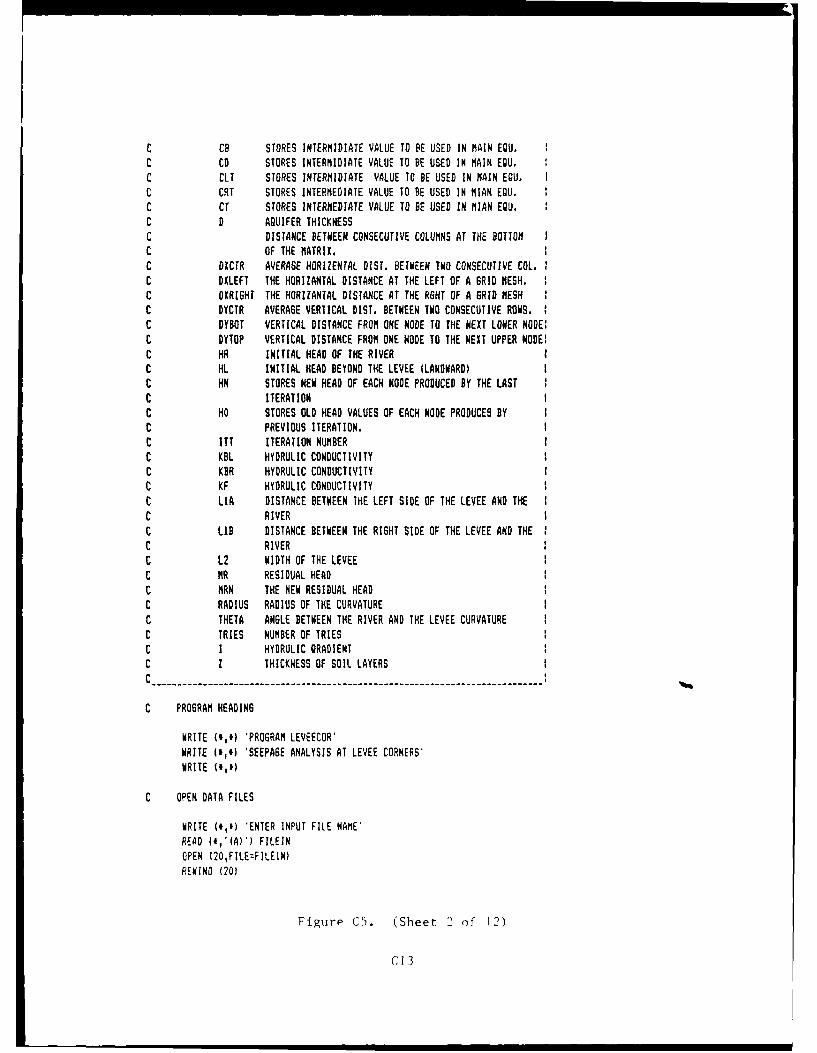
SCB STORES INTERMIDIATE VALUE TO BE USED IN MAIN EIU IC CD STORES INTERMIDIATE VALUE TO BE USED IN MAIN EQU.C CL STORES INTERMIDIATE VALUE TO BE USED IN MAIN EU. IC CRT STORES INTERMEDIATE VALUE TO BE USED IN MIAN EQU.C CT STORES INTERMEDIATE VALUE TO BE USED IN MIAN EQU.C 0 AQUIFER THICKNESSC DISTANCE BETWEEN CONSECUTIVE COLUMNS AT THE BOTTOM IC OF THE MATRIX. IC DlCrR AVERAGE HORIZENTAL DIST. BETWEEN TWO CONSECUTIVE COL. 1C DXLEFT THE HORIZANTAL DISTANCE AT THE LEFT OF A GRID MESH. 1C OXRIGHr THE HORIZANTAL DISTANCE AT THE RBHT OF A GRID MESHC DYCTR AVERAGE VERTICAL DIST. BETWEEN TWO CONSECUTIVE ROWS.C DYBOT VERTICAL DISTANCE FROM ONE NODE TO THE NEXT LOWER NODE!C DYTOP VERTICAL DISTANCE FROM ONE NODE TO THE NEXT UPPER NODE!C HR INITIAL HEAD OF THE RIVER IC HL INITIAL HEAD BEYOND THE LEVEE (LANDWARD) IC HN STORES NEW HEAD OF EACH NODE PRODUCED BY THE LASTC ITERATIONC HO STORES OLD HEAD VALUES OF EACH NODE PRODUCES BYC PREVIOUS ITERATION.C ITT ITERATION NUMBER IC KBL HYDRULIC CONDUCTIVITYC KBR HYDRULIC CONDUCTIVITY IC KF HYDRULIC CONDUCTIVITYC LIA DISTANCE BETWEEN THE LEFT SIDE OF THE LEVEE AND THE IC RIVER IC LID DISTANCE BETWEEN THE RIGHT SIDE OF THE LEVEE AND THE 1C RIVERC L2 WIDTH OF THE LEVEEC MR RESIDUAL HEADC MRN THE NEW RESIDUAL HEADC RADIUS RADIUS OF THE CURVATURE
C THETA ANGLE BETWEEN THE RIVER AND THE LEVEE CURVATUREC TRIES NUMBER OF TRIESC I HYDRULIC GRADIENTC I THICKNESS OF SOIL LAYERS IC ----------------------------------------------------------------------------
C PROGRAM HEADING
WRITE (I,*) 'PROGRAM LEVEECOR'WRITE ('i') 'SEEPAGE ANALYSIS AT LEVEE CORNERS'WRITE (#,)
C OPEN DATA FILES
WRITE (*,,) 'ENTER INPUT FILE NAME'
READ (4,'(A)'1 FILEINOPEN 120,FILE=FILEIN)REWIND (20)
Figure C5. (Sheet 2 of 12)
C13
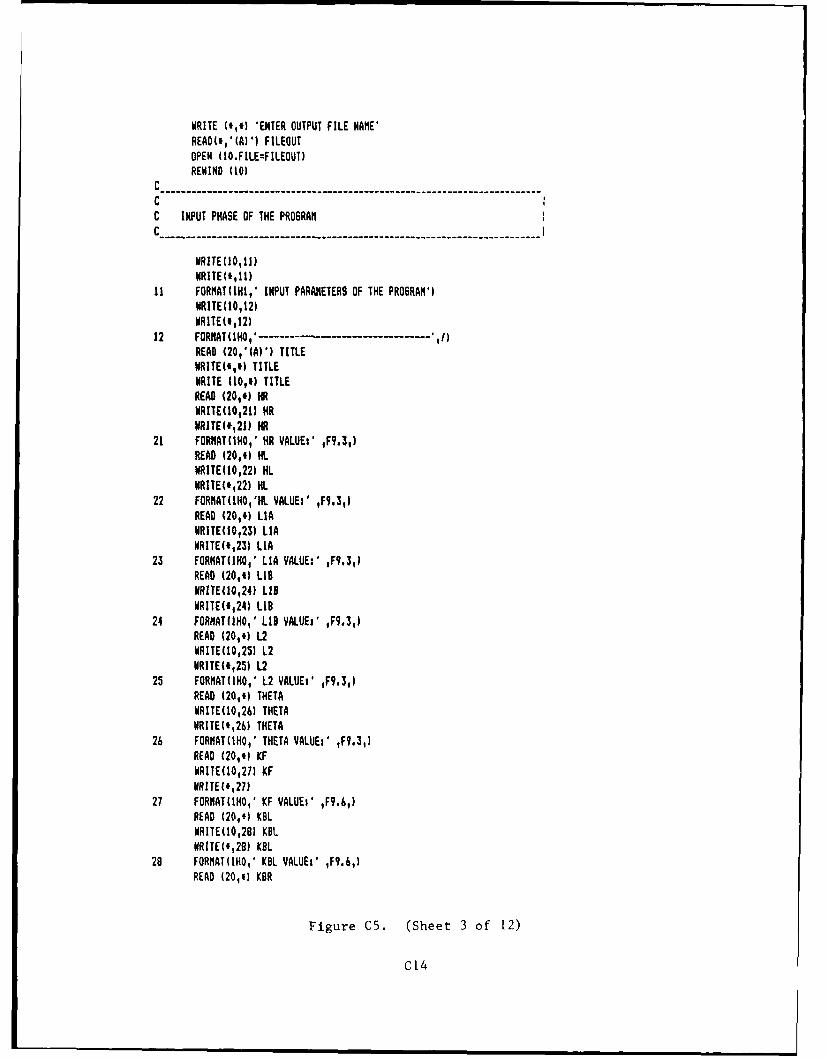
WRITE (yI,) 'ENTER OUTPUT FILE NAME'
READ(*,'(A)') FILEOUTOPEN (IO.FILE=FILEOUT)
REWIND (10)C-------------------------------------------------C
C INPUT PHASE OF THE PROGRAM
WRITE(10,1])WRITE(t,11)
11 FORNAT(IHI,' INPUT PARAMETERS OF THE PROGRAM')WRITEIOl,12)
WRITE(I,12)12 FORMAT(IHO-' ----- -
READ (20,'(A)') TITLEWRITE(.,') TITLEWRITE (10,) TITLEREAD (20,4) HWRITEO,21) HRWRITE(0121) HR
21 FORMAT(INO,' HR VALUEs' ,F9.3,)READ (20,) HILWRITE(10,22) HLWRITE(0,22) HL
22 FORMAT(IHO,'HL VALUE:' ,F9.3,)READ (20,4) LIAWRITE(10,23) LIA
WRITE(*,23) LIA23 FORNAT(IKO, ' LIA VALUE:' ,F9.3,)
READ (20,) LIDWRITE(10,24) LIDWRITE(4124) LID
24 FORMATIIHO,' LID VALUE:' ,F9.3,)READ (20,0) 12WRITE(tO,25) L2WRITE(0,25) L2
25 FORMATQIHO,' L2 VALUEr' ,F9.3,)READ (20,) THETAWRITE(10,26) THETAWRITE(0,26) THETA
26 FORMAT(IHO,' THETA VALUEs' ,F9.3,)READ (20,) KF
WRITE(10,27) KFWRITE(0,27)
27 FORMAT(IHO,' KF VALUEs' ,F9.6,)READ (20,) KBLWRITE(tO,261 KBLWRITE(0,28) KBL
28 FORMAT(IHO,' KBL VALUEr' ,F9.6,)READ (20,.) KBR
Figure C5. (Sheet 3 of 12)
C14

MRITE(10,29) KBRWRITE(#,29) KDR
29 FORMAT(IHO,' KBR VALUE: ,F9.6,)READ (20,4) RADIUSWRITE(10,30) RADIUSWRITE(0,30) RADIUS
s0 FORMAT(IHO,' RADIuS YALUEt' ,F9.3,)READ (20,#) 0WRITE(10,31) DWRITE(0,31) D
31 FORHAT(IHO,' VALUEi' ,F9.31)READ (20,01 TOLNRITE(00,32) TOL
WRITE(4,32) TOL
32 FORMAT(IHO,' TOL VALUEt' ,F9.6,)READ (20,) TRIESWRITE(10,33) TRIES
WRITE(e,3) TRIES33 FORMAT(IHO,' TOTAL NUDER OF TRIES',15,)
READ (20,) ZWRITE (10,34) 1WRITE(0134) Z
34 FORMAT(IHO,' THICKNESS VALUEa' ,F12.6,)
CCC INITIALIZATION PHASE OF THE PROGRAM
C CONVERT THETA TO RADIANS
THETA=THETA/57.29578
C INITIALIZE HEADS
DO 40 RzO,7H(RI,)zOH(R,16)=O
IF (R.LE.3) THENHD(R)=HL
ELSEHD(R)HR
ENDIF
40 CONTINUE
DO 44, C=1,15H(7,C)=0H(6,C):HRH(I,C)-HL
Figure C5. (Sheet 4 of 12)
C15
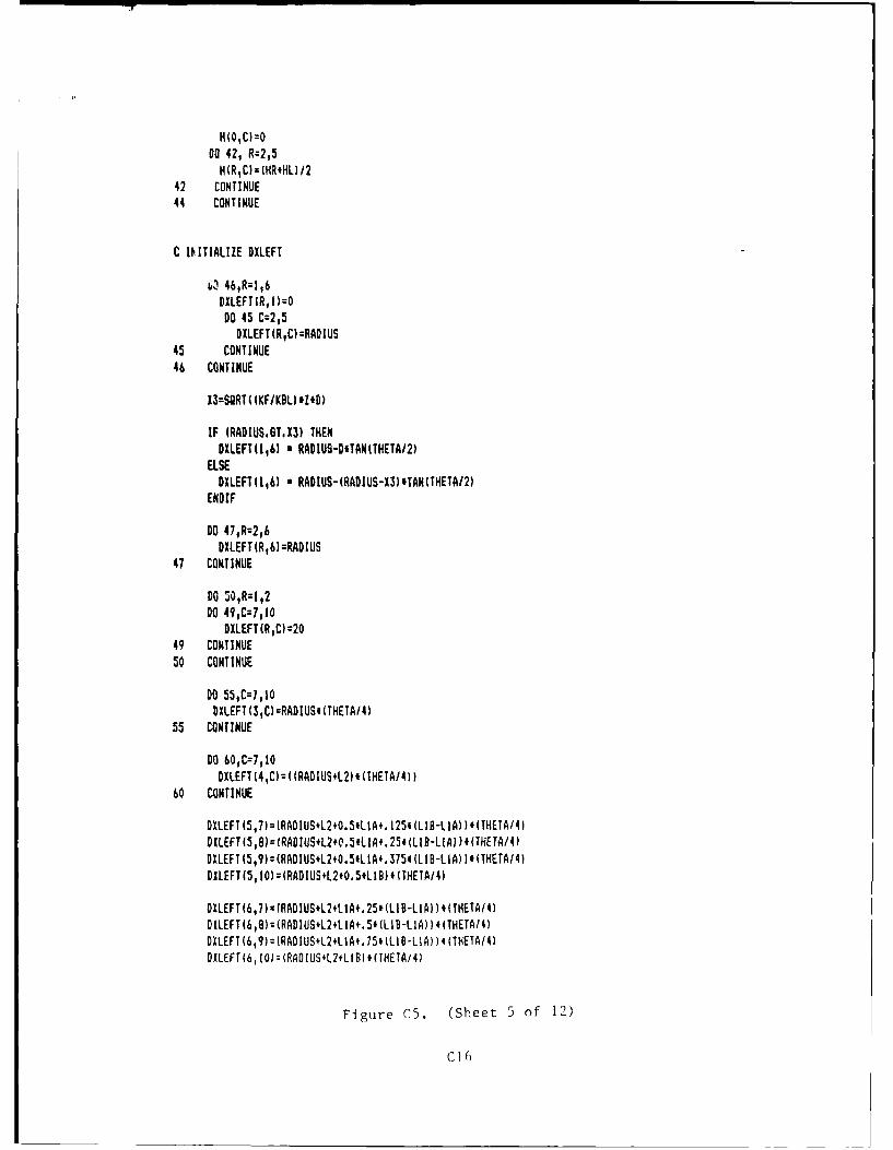
HioICkO=00 42, R=2,5H(R,Ckr(HR+HL)/2
42 CONTINUE44 CONTINUE
C IIALIlE DXLEFT
&3 46,R=1,6DXLEFTIR,I)=000 45 C=215
DXLEFT(R,C) :RADIUS45 CONTINUE46 CONTINUE
13:SQRT ((KFIKDU *2*0)
IF (RADIUS.6T1 3) THENDXLEFT(116) a RADIUS-D#TAN(THETA/2)
ELSEDXLEFT1116) a RADIUS-(RADIUS-X3)*TAN(THETA/2)
ENDIF
DO 47,R=2,6DILEFT(R,6)=RADIUS
47 CONTINUE
DO 50,R=1,20O 49,C=7,I0
DXLEFT(R,C) :2049 CONTINUE50 CONTINUE
DO 55,C=7,10DXLEFT(3,C)=RADIUSI (THETAl4)
55 CONTINUE
DO 60,C=7,10DXLEFT(4,C)=((RADIUS+L2).(THETAI4))
60 CONTINUE
DXLEFT(5,7):(RADIUS+L2+0.5.LIA+. 125'(LIB-LIA))*(THETA/4)DILEFT(5,6):(RADIUS+L2,Q.5.LlA..25#(LIB-LIAI)e#(THETA/4)DXLEFT(5,9):-(RADIUS+L2+0.5ILIA+.375#(LIB-LIAl*(THETA/4)DILEFT(5, I0)=(RADIUS+L2+0.5ILIB) *CTHETA/4)
DXLEFT(6,7)x(RADIUS+L2+LIA+.25i(LIB-LIAI ).(THETA/4)DXLEFT(6,8)=(RADIUS+L2,L1A+.5#(LIE-LIA) ).(THETAI4)DXLEFT(6,9)h(RADIUS+L2+LiA+.75'(LIB-LIA) ).(THETA/4)DXLEFT(6, I0i:(RADIUS4L2+t(BI .(THErA/4)
Figure C5. (Sheet 5 of 12)
C 16
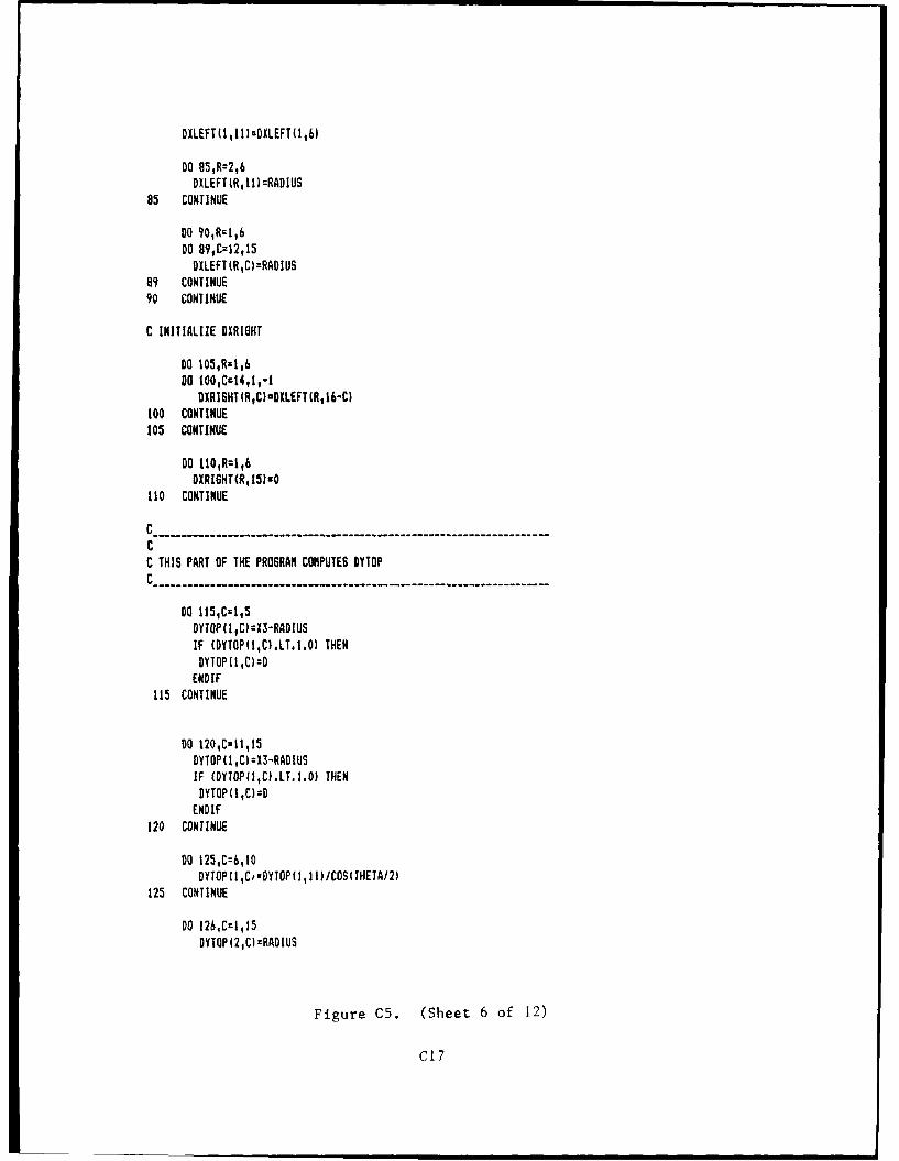
DXLEFT(I,II)lDXLEFT(I1,6)
O0 85,R=2,6DXLEFTiR,11)=RADIUS
85 CONTINUE
DO 90,R=1,6DO 89fC=12,15DXLEFT(RC)=RADIUS
89 CONTINUE90 CONTINUE
C INITIALIZE XRIGHT
DO 105,R-1,6DO 100,Cu14,1,-1
DXRIGHT(RC)=DXLEFT(R,16-C)100 CONTINUE105 CONTINUE
DO 110,R:1,6DXRIGHT(R,15)g0
110 CONTINUE
CCC THIS PART OF THE PROGRAM COMPUTES DYTOP
DO 115,C=1,5DYTOP(IC):X3-RADIUSIF (DYTOP(1,C).LT.I.0) THENDYTOP(IC):D
ENDIF115 CONTINUE
DO 1201Ci11,15DYTOP(1,C)=13-RADIUSIF (DYTOP(1,CI.LT.I.0) THENDYTOP(I,C)=D
ENDIF120 CONTINUE
DO 125 ,C=6,10DYTOPIICtsDYTOP(li)/COS(THETA/2)
125 CONTINUE
DO 126,CI,15DYTQP(2,C) RADIUS
Figure C5. (Sheet 6 of 12)
C17
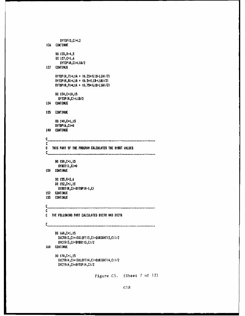
DYTOP13 1C)=L2126 CONTINUE
DO 135,R=4,500 127,C=116
DYTOPIRC)=LIAI2127 CONTINUE
DYTOP(R,7)=LIA 4 (0.25*(LIB-LIAI/2)
DYTOP(R,B).IA + (0.50(LIB-LIA)/2)DYTOP(R,9)LIA * (0.75e(LIB-LIA)I/2)
O0 134,C:10,15DYTOP(RlC)=IIB/2
134 CONTINUE
135 CONTINUE
DO 140,C:I,15
DYTOP(6,C)'-O
140 CONTINUE
CCC THIS PART OF THE PROGRAM CALCULATES THE DYBOT YALUES
C ----------------------------------------------
DO 1501C21,15DYBOT(IC)-O
150 CONTINUE
DO 155,R=2,6DO 152,C'1,15
DYBOT(RC)=DYTOP(R-IC)152 CONTINUE135 CONTINUE
CC THE FOLLOWING PART CALCULATES DICTR AND DYCTR
C .............................----..............--..................
DO 160,C21,15DICTR(3,C)=(DXLEFT(3,C)+DXRIGHT(3,C))/2DYCTR(3,C)=DYBOT(3,C)/2
160 CONTINUE
DO t7OCzlit5DXCTR(4,C)z(DXLEFT(4,C)+DXRi6HT(4,C))/2
OYCTR(4,C)=DYTOP(4,C)I2
Figure C5. (Sheet 7 of 12)
C18
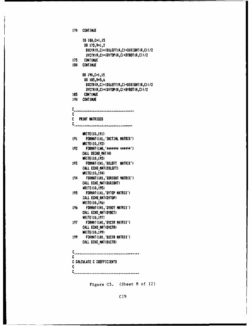
170 CONTINUE
DO 180,Ccl,15DO 175,Ral,2DXCTR(R,C)x(DXLEFT(R,C)4DXRIBHT(RC) )12DYCTR(RCc1DYTOP(R,C)+DYDOT(RC) I/2
175 CONTINUE180 CONTINUE
DO 1901C:1,15DO 185,RR5,&DXCTR(RC)z(DXLEFT(R,C)+DXRIGHT(RC) )12DYCTR(RC)u(DYTOP(RC)+DYDOT(RC) 1/2
185 CONTINUE190 CONTINUE
C............C --- --- -- --- ---- --C PRINT MATRICESC --- -- --- ---- -- ---
WRITE 0, 191)191 FORMAT(IHI,'INITIAL MATRIX-)
WRITE( 00 192)192 FORMAT(IHO'*#**n*11*'
CALL DECHO MATIN)WRITE(10, 195)
193 FORMNATI4I'LEFT MATRIX-)CALL ECHONMAT(DILEFT)WRITE 0, 194)
194 FORMATI1H1,'DXRIBHT MATRIX-)CALL ECHO HAT (DXRIBHT)WRITE(0,195s)
195 FORMAT(IHII4DY70P MATRIX')CALL ECHO MAT (DYTOP)WRITE (0,196)
196 FORMAT(INII-DYBOT MATRIX')CALL ECHO HAT(DYSOT)WRITECIO, 97)
197 FORMAT(III-DYCTR MATRIX-)CALL ECHO MAT (DYCTR)WRITE0, 199)
199 FORMAT(IHI,'DXCTR MATRIX-)CALL ECHODMAT (DX CTR)
C CALCULATE C COEFFICIENTSCC --- --- -- --- --- ---- -
Figure C5. (Sheet 8 of 12)
C19
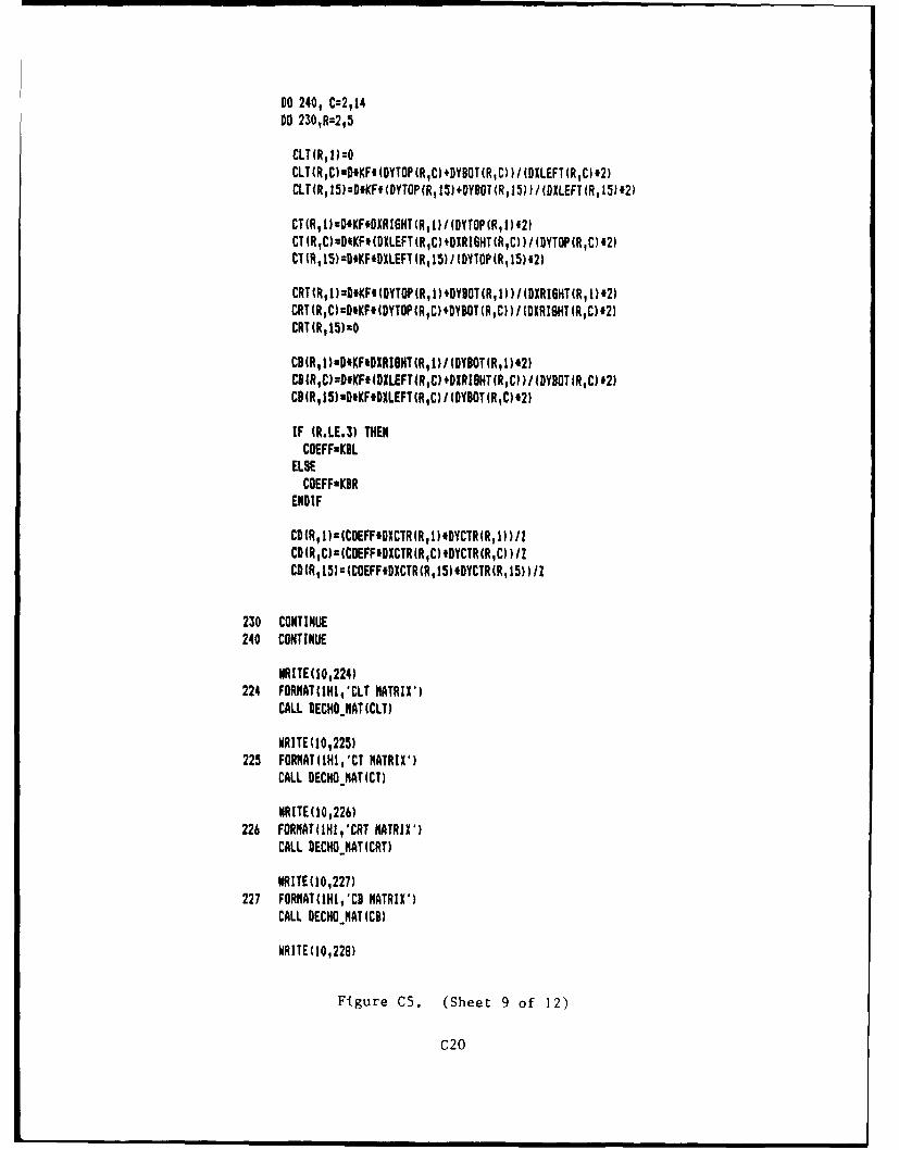
0240, C:2114DO 230,R=2,5
CLT(R,I)=0CLT(R,C).D'KF4(DYTOP(RC)+DYBOT(RC) )I(DXLEFT(RC).2)CLr(R,15)=D.KF.(DYTOP(R,15)+DYDQT(R,15) )/(DXLEFT(R, 15)12)
CT (A, 1) DIKFIOXR IGHT (A,1)/1(DYTOP (R,1) 2)CT(RfC):D*KF.(DXLEFT(RC)4DXRIGHT(R,C) )/(DYTOP(R,C)#2)
CRT(R,1).D*KF#(DYTOP(R,1).DYDOT(R,1)/)IDXRIGHT(R,1)42)CRTCR,C)r.D'KF.(DYT0P(RC).DYBOT(R,C) )I(DXRIBHT (RC)42)CRT (A, 15)%
CD(R,1)uD*KF'DXRIGHT(R,1)/(DYBOT(R,1).2)CBIR,C):D*KF*(DXLEFTIC)+DXRISHT(RC) )/IDYBOTIR,C) '2)CDIR, 15)uD*KF.DXLEFT (RC)/I(DYDOTIRC)'2)
IF (R.LE.3) THENCOEFFmKDL
ELSECOEFFxKDR
ENDIF
CD(R,1)cCEFFDXCTRA,1.)DYCTR(R,1nh/ZCD1RC)z(COEFF'DXCTRR,C)#DYCTAR,C) ) ICD(A115)u(COEFF#DXCTR(R,1S).DYCTR(R,15 )Il
230 CONTINUE240 CONTINUE
WRITE(10,224)224 FORNAT(IHIICLT MATRIX)
CALL DECHONHAT (CLT)
WRITE(10,225)225 FORMATlIHI,'CT MATRIX)
CALL DECHO NAT (CT)
WRITE( 0,226)226 FORMAT(iHI,'CRT MATRIX')
CALL DECHOHAT (CAT)
WRITE(10,227)227 FORMAT(IHI,'CD MATRIX-)
CALL DECHOHAT (CB)
WRITE( 0,228)
Figure C5. (Sheet 9 of 12)
C20
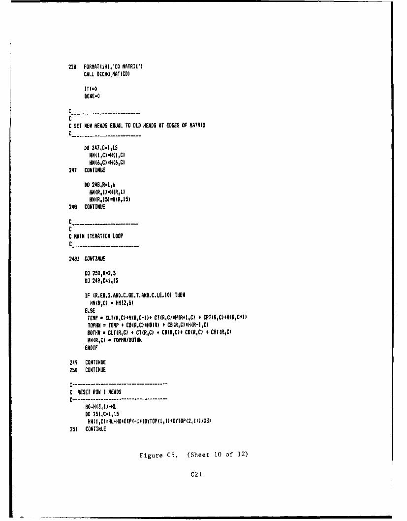
228 FORMAT(IHI,'CO MATRIX-)CALL DECHOMAT (CD)
ITT=ODONE=O
Cc - - - -- - - - - - -- -C SET NEW HEADS EQUJAL TO OLD HEADS AT EDGES OF MATRIXC - - - - - --- --- - -
DO 247,C'I,15
HN(6,C)zII(6Cl247 CONTINUE
DO 2481RxI,6UN (R, I )H(R, 1)HNlR, 15) 1$(R,I5)
249 CONTINUE
C ----------------CC MAIN ITERATION LOOP
2481 CONTINU)E
DO 250,R:2,5
DO 249,CzI,15
IF (R.EG.2.AND.C.BE.7.ANlD.C.LE.IO) THENN(R,C) x N12,6)
ELSETEMP z CLT(RICIEH(R,C-l)* CT(R,C)#H(R*1,C) + CRTIR,C)#HIR1C*1)TOPHN z TEMP + CD(RfC)#HD(R) + CB(RfC),H(R-I,C)BOTHN s CLT(RC) # CT(R,C) + CB(R,C). CD(RC) + CRTIR,C)HN(R,C) a TOPHNIBOTHN
ENDIF
249 CONTINUE250 CONTINUE
C-----------------------C RESET ROW I HEADSC ------------------------------
HOmmH(3,I)-HLDO 251,Cz~qI5HN(11C):HL4HO4EIP(-II(DYTOP(I,I)4DYTOP(2,IJ)113)
251 CONTINUE
Figure C5. (Sheet 10 of 12)
C21
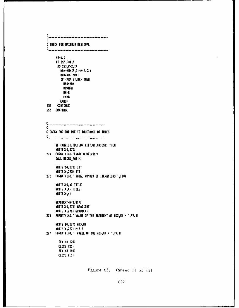
C - - -------------- -----CC CHECK FOR MAXIMUM RESIDUALC --------------------------
MR:O.ODO 255,R=1,6DO 253,Cn2,14NRN=(HNIRIC)-H(RC))MRA:ABS(MRN)IF (IRA.GT.MR) THENNRX:MRNMR:MRARM=R
ENDIF253 CONTINUE255 CONTINUE
CC
C CHECK FOR END DUE TO TOLERANCE OR TRIESC___
IF ((MR.LT.TOL).OR.(ITT.BT.TRIES)) THEN
NRITE(I0,270)270 FORNAT(IHII'FWNAL H MATRIX-)
CALL DECHO.MAT(H)
NRITE(IO,275) ITT
NRITE(4,275) ITT275 FORMAT(IHO,' TOTAL NUMBER OF ITERATIONS '1IIO)
NRITE(IO,') TITLEURITE(COl TITLE
NRITE(00)
GRADIENTzH(3,8)IZWRITE(I0,276) GRADIENT
WRITE(0,276) GRADIENT276 FORNAT(IHO,' VALUE OF THE GRADIENT AT H(3,8) z ',F9.4)
WRITE(O1,277) H(318)WRITE(.,277) H(3,8)
277 FORMAT(IHO,' VALUE OF THE H(3,O) a ',F9.4)
REWIND (20)CLOSE (20)REWIND (10)CLOSE (10)
Figure C5. (Sheet 11 of 12)
C22
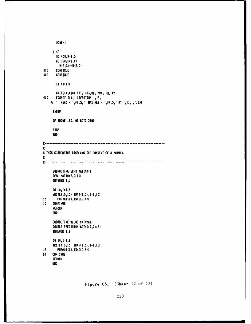
DONE=!
ELSEDO 400,R=1,5DO 300,C=1,15H(RC)=HN(RC)
300 CONTINUE400 CONTINUE
ITT=ITTtI
WRITE(0,410) ITT, HI3,B), NRX, RN, CM410 FORMAT (II,' ITERATION ',15,
&' HEAD a ',F9.5, MX RES x *,F9.5,' AT ,13,',13)
ENDIF
IF (DONE .E9. 0) GOTO 2491
STOPEND
CC THIS SUBROUTINE DISPLAYS THE CONTENT OF A MATRIX.C
SUBROUTINE ECHO.MAT(NAT)REAL NAT(0a1,0t16)INTE6ER IJ
DO 10,12:16WRITE(10,15) (MAT(IJ)J):1,l5)
15 FORMAT(1I,15(610.4))10 CONTINUE
RETURNEND
SUBROUTINE DECHO NAT(MAT)DOUBLE PRECISION hAT(0:7,0il6)INTEGER IJ
DO 10,1:1,6WRITE(00,15) (flAT(I,J),J:I,15)
15 FORMAT(IX,15(S10.4))10 CONTINUE
RETURNEND
Figure C5. (Sheet 12 of 12)
C23
APPENDIX D: COMPARISON OF PROGRAMS
Example Problem
1. In this appendix, a comparison is made among the solutions obtained
for a common example problem using the computer programs LEVEE3L, LEVEEIRR,
LEVEECOR, and the conventional method. The example selected is the same as
that used for Figure 45 in the main text. Foundation conditions are assumed
to consist of a 10-ft-thick top blanket overlying an 80-ft-thick substratum.
The ratio of the horizontal substratum permeability to the vertical top
blanket permeability is assumed to be 1,000. The foundation is assumed to
extend 1,500 ft riverside of the levee to an open seepage entrance. The levee
base width is assumed to be 300 ft. The foundation is assumed to extend
infinitely in the landside direction. The calculated residual head at the
levee toe using the conventional method is 8.97 ft.
Comparative Solutions
2. The heads obtained using the computer analyses and conventional
analyses are plotted as a function of horizontal distance in Figure D1.
Computer solutions for the residual head at the levee toe range from 6.6 to
8.9 ft, a difference of 2.3 ft. Two different segment assumptions are shown
for LEVEEIRR in Figure Dl. Computer solutions in this example reflect
generally lower heads than the conventional solution, a trend also noted in
the case studies cited in the main report. These variations are larger than
was generally expected at the outset of the research. Reasons for these
variations are not completely understood at the time of preparing this report;
there are, a number of factors that may contribute. These are discussed
below.
Differences in Program Assumptions
3. The programs and the conventional method employ certain fundamen-
tally different assumptions to derive the flow equations. In the conventional
method, flow is assumed to be horizontal in one direction in the substratum
and is assumed to be vertical in the top stratum. In LEVEE3L, both
DI
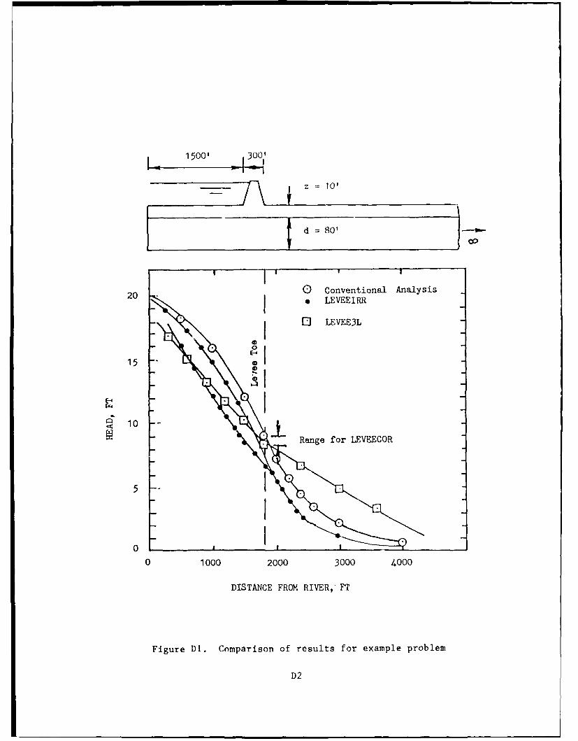
1500' 300'
0 Conventional Analysis20 • LEVEEIRR
[ EVEE3L
E-
154
10 - "
Range for LEVEECOR
0 1000 2000 3000 4000
DISTANCE FROM RIVER, FT
Figure D1. Comparison of results for example problem
D2
horizontal and vertical flow is accounted for in each of three layers. In
LEVEEIRR, flow assumptions are generally the same as the conventional solu-
tion, but the flow equation is still satisfied only approximately at a finite
number of points rather than exactly at all points. In LEVEECOR, flow in the
substratum is horizontal only, but has two horizontal components, and flow in
the top stratum is vertical only. In LEVEE3L and LEVEEIRR, boundaries at an
infinite distance must be modeled by using rather large finite distances.
Results will vary depending on the boundary distance specified. In LEVEECOR,
which most closely matched the conventional solution at the levee toe, the
head on the landside boundary is forced to be consistent with the conventional
closed-form solution.
Numerical Problems Common to All Programs
4. In each of the three programs, the solution is obtained by itera-
tion. As the tolerance is made smaller and the number of iterations is
increased, a more accurate solution is expected. However, this may not always
be the case as round-off errors may accumulate where the tolerance or maximum
allowable residual is set extremely low. Recommended tolerance values based
on limited experience with the programs are given in Appendices A through C.
Associated with any finite difference solution is a discretization or trunca-
tion error, due to the fact that a continuous system is replaced with a finite
system. For the three computer programs developed, the gradients at a node
point are represented by a first-order approximation of the derivative of head
with respect to distance. The truncation errors could conceivably be reduced
and more accurate solutions obtained if higher order approximations were used
or if node spacing was significantly reduced. Both of these approaches would
increase program complexity or execution time. The present research was
viewed as an initial evaluation of the utility of applying numerical methods
to underseepage analysis and involved a deliberate effort to produce working
versions of three different programs that were fundamentally as simple as
possible.
D3

APPENDIX E: NOTATION
c A constant; inverse of the effective exit distance
d Thickness of pervious substratum
h Residual head at levee toe0
h Net head at distance x landward of levee toexH Net head on levee
kb Permeability of top blanket
l Permeability of landside top blanket
kbr Permeability of riverside top blanket
kf Permeability of pervious substratumkfh Horizontal permeability of top blanket in three layer system
k V Vertical permeability of top blanket in three layer system
k2h Horizontal permeability of middle stratum in three layer system
k2v Vertical permeability of middle stratum in three layer system
k3h Horizontal permeability of substratum in three layer system
k3v Vertical permeability of substratum in three layer system
Lk Distance from riverside toe of levee to open or blocked seepage
entranceL2 Distance from riverside toe of levee to landside toe
L3 Distance from landside toe of levee to open or blocked seepage exit
q Flow
s Distance from landside levee toe to effective seepage entrance
x I Distance from riverside toe of levee to effective seepage entrance
L2 Distance from riverside toe of levee to landside toe
x3 Distance from landside toe of levee to effective seepage exit
z Thickness of top blanket
zI Thickness of top blanket in three-layer system
z 2 Thickness of middle stratum
El
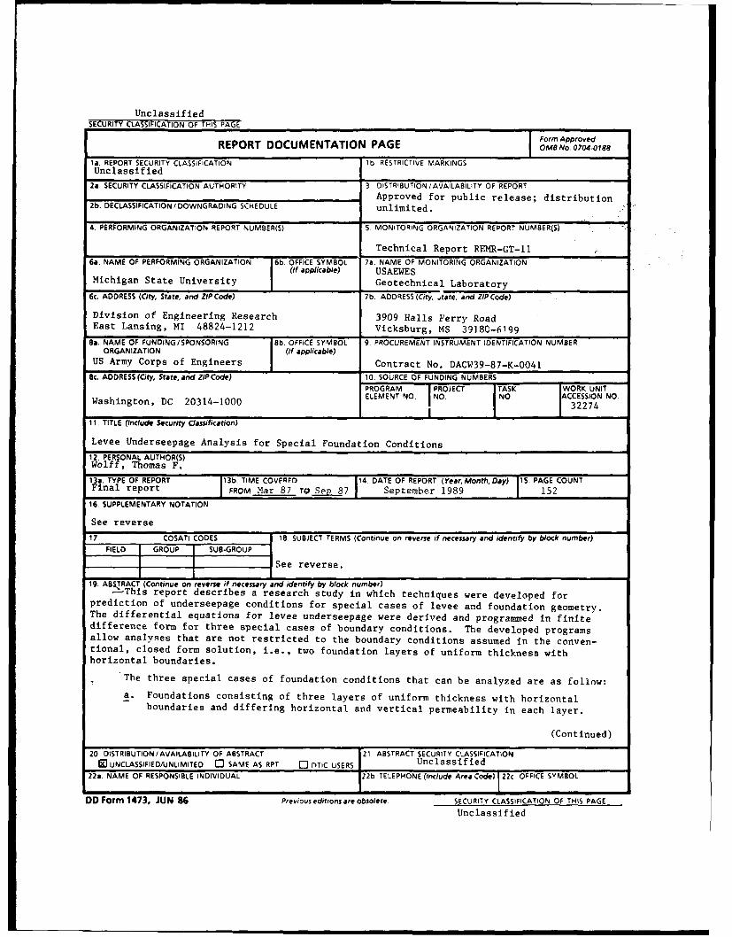
UnclassifiedSECURITY CLASSIFICATION OF THIS PAGE
Form Approved
REPORT DOCUMENTATION PAGE OMBNo. r 704.r18e
Ia. REPORT SECURITY CLASSIFICATION lb RESTRICTIVE MARKINGSUnclassified
2a. SECURITY CLASSIFICATION AUTHORITY 3 DISTRIBUTION /AVAILABILITY OF REPORTApproved for public release; distribution
2b. DECLASSIFICATION /DOWNGRADING SCHEDULE unlimited.
4. PERFORMING ORGANIZATION REPORT NUMBER(S) S. MONITORING ORGANZATION REPORT NUMBER(S)
Technical Report REMR-GT-11
6a. NAME OF PERFORMING ORGANIZATION 6b. OFFICE SYMBOL 7a. NAME OF MONITORING ORGANIZATION(If applicable) USAEWES
Michigan State University Geotechnical Laboratory
6c. ADDRESS (City, State, and ZIP Code) 7b. ADDRESS (City, Jtate, and ZIP Code)
Division of Engineering Research 3909 Halls Ferry RoadEast Lansing, MI 48824-1212 Vicksburg, MS 3918C-6199
Ba. NAME OF FUNDING/SPONSORING 8b. OFFICE SYMBOL 9. PROCUREMENT INSTRUMENT IDENTIFICATION NUMBERORGANIZATION (If applicable)
US Army Corps of Engineers Contract No. DACW39-87-K-0041
Sc. ADDRESS(City, State, and ZIP Code) 10. SOURCE OF FUNDING NUMBERSPROGRAM I PROJECT ITASK WORK UNITELEMEN NO N. NO. ACCESSION NO.
Washington, DC 20314-1000 E N 32274
11. TITLE (Include Security Classification)
Levee Underseepage Analysis for Special Foundation Conditions
12. PERSONAL AUTHOR(S)Wolff, Thomas F.
13a. TYPE OF REPORT 13b. TIME COVFRFO 14. DATE OF REPORT (Year, Month, Day) 15. PAGE COUNTFinal report FROM Mar 87 TO Sep 87 September 1989 152
16. SUPPLEMENTARY NOTATION
See reverse
17. COSATI CODES 18 SUBJECT TERMS (Continue on reverse if necessary and identify by block number)FIELD GROUP SUB-GROUP
See reverse.
19. ABSTRACT (Continue on reverse if necessary and identify by block number)-This report describes a research study in which techniques were developed for
prediction of underseepage conditions for special cases of levee and foundation geometry.The differential equations for levee underseepage were derived and programmed in finitedifference form for three special cases of boundary conditions. The developed programsallow analyses that are not restricted to the boundary conditions assumed in the conven-tional, closed form solution, i.e., two foundation layers of uniform thickness withhorizontal boundaries.
The three special cases of foundation conditions that can be analyzed are as follow:a. Foundations consisting of three layers of uniform thickness with horizontal
boundaries and differing horizontal and vertical permeability in each layer.
(Continued)
20 DISTRIBUTION/AVAILABILITY OF ABSTRACT 21 ABSTRACT SECURITY CLASSIFICATION-UNCLASSIFIEDIUNLIMITED 0 SAME AS RPT ODTIC USERS Unclassified
22a. NAME OF RESPONSIBLE INDIVIDUAL 22b TELEPHONE (Include Area Code) 22c OFFICE SYMBOL
DD Form 1473, JUN 86 Previous editions are obsolete SECURITY CLASSIFICATION OF THIS PAGEUnclassified
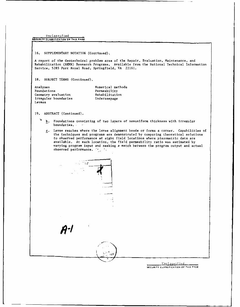
UnclassifiedIECUMI1Y CLAUIFICATION OF TWII PAGE
16. SUPPLEMENTARY NOTATION (Continued).
A report of the Geotechnical problem area of the Repair, Evaluation, Maintenance, andRehabilitation (REMR) Research Programs. Available from the National Technical InformationService, 5285 Port Royal Road, Springfield, VA 22161.
18. SUBJECT TERMS (Continued).
Analyses Numerical methodsFoundations PermeabilityGeometry evaluation RehabilitationIrregular boundaries UnderseepageLevees
19. ABSTRACT (Continued).
b. Foundations consisting of two layers of nonuniform thickness with irregularboundaries. -
c. Levee reaches where the levee alignment bends or forms a corner. Capabilities ofthe techniques and programs are demonstrated by comparing theoretical solutionsto observed performance at eight field locations where piezometric data areavailable. At each location, the field permeability ratio was estimated byvarying program input and seeking a match between the program output and actualobserved performance. > ,
SECURtY CLASSIFICATION OF T1IS PAGE