@let@token Bayesian Calibration of Simulators with ... · Bayesian Calibration of Simulators with Structured Discretization Uncertainty Oksana A. Chkrebtii Department of Statistics,

cal i brat i on w ith d i s cret i z at i on uncerta i nty ok sana chkrebt i i

Bayesian Calibration of Simulators with StructuredDiscretization Uncertainty

Oksana A. ChkrebtiiDepartment of Statistics, The Ohio State University

Joint work with Matthew T. Pratola (Statistics, The Ohio State University)

Probabilistic Scientific Computing: Statistical inference approaches to numericalanalysis and algorithm design, ICERMJune 7, 2017

Slide 1/29


Probabilistic Numerics

This is an active new field that challenges historical perspectives onnumerical analysis.

It is important for this community to develop new methods with an eyeto overcoming challenges that lay ahead.

This talk focuses on calibration for forward problems defined by thesolution of ordinary and partial differential equations. If you’re notalready convinced that probabilistic numerics is useful in this setting ...

Slide 2/29


Example - galaxy simulation (Kim et al., 2016)

Slide 3/29


Example - galaxy simulation (Kim et al., 2016)

• These are not realizations of a field (the model is deterministic)

• The initial conditions and inputs are held fixed

• How do we evaluate these numerical solver outputs?

Slide 4/29


Perspectives on Probabilistic Numerics

Probability measures on numerical solutions via randomization

• Conrad et al (2015/16), Lie et al (2017)

• defined outside of the Bayesian framework, but resulting algorithmsoverlap

Bayesian uncertainty quantification for differential equations

• Skilling (1991), Chkrebtii et al (2013/16), Arnold et al (2013)

• defined outside of the numerical analysis framework, but resultingmethods can be analogous in some sense

Bayesian numerical methods

• Hennig & Hauberg (2013/14), Schober et al (2014).

• computationally efficient probabilistic GP based methods; canrecover numerical solvers in the mean

Slide 5/29


Calibrating stochastic computer models

Regardless of the perspective, the deterministic but unknown forwardmodel is replaced by a stochastic process: for fixed inputs, the output isa random variable with (often) unknown distribution.

Pratola & Chkrebtii (2017+) describe a hierarchical framework tocalibrate stochastic simulators with highly structured outputuncertainty/variability.

Slide 6/29


Calibration problem

We wish to estimate the unknowns, θ ∈ Θ, given observations,

y(xt) = A {u(xt , θ)}+ ε(xt), xt ∈ X , t = 1, . . . ,T ,

of the deterministic state ut = u(xt , θ) transformed via an observationprocess A, and contaminated with stochastic noise ε.

The likelihood defines a discrepancy between the model and the data:

f (y1:T | θ) ∝ ρ {y1:T − A (u1:T )}

Slide 7/29


The Bayesian paradigm

Bayesian inference is concerned with modeling degree of belief about anunknown quantity via probability models.

For example, we may not know θ ∈ Θ but we may have some prior beliefabout, e.g., its range, most probable values,

θ ∼ π(θ).

We seek to update our prior belief by conditioning on new information,y1:T ∈ Y, e.g., data, model evaluations, via Bayes’ Rule:

p(θ | y1:T ) =p(y1:T | θ)π(θ)∫p(y1:T | θ)π(θ) dθ

∝ p(y1:T | θ)π(θ).

Slide 8/29


A Hierarchical model representation

Hierarchical modelling enables inference over the parameters of astochastic state,

[y1:T | u1:T , θ] ∝ ρ {y1:T − A (u1:T )}

[u1:T | θ] ∼ p(u1:T | θ)

[θ] ∼ π(θ).

When p(u1:T | θ) is not known in closed form, exact inference may stillbe possible via Monte Carlo, using forward-simulation from the model.However, this is often computationally prohibitive.

Slide 9/29


For probabilistic numerics

If the state is deterministic but defined implicitly by a system ofdifferential equations, our uncertainty about the solution can be modelledprobabilistically,

[y1:T | u1:T , θ] ∝ ρ [y1:T − A (u1:T )]

[u1:T | θ] ∼ a probability measure representing uncertaintyin the solution given discretization of size N

[θ] ∼ π(θ).

We use the Bayesian uncertainty quantification approach to model thismiddle layer.

Slide 10/29


Bayesian UQ for differential equations

Given θ and for linear operator D consider the initial value problem,{Du = f (x , u) , x ∈ X ,u = u0 x ∈ ∂X .

We may have some prior knowledge about smoothness, boundaryconditions, etc., described by a prior measure,

u ∼ π, x ∈ X

We seek to update our prior knowledge by conditioning on modelinterrogations, f1:N via Bayes’ Rule,

p(u(x) | f1:N) =p(f1:N | u(x))π(u(x))∫

p(f1:N | u(x))π (u(x)) du(x)∝ p (f1:N | u(x)) π (u(x))

Slide 11/29


Prior uncertainty in the unknown solution

The exact solution function u is deterministic, but unknown. We maydescribe our prior uncertainty via a probability model defined on thespace of suitably smooth derivatives, e.g.,

u ∼ GP(m0,C 0), m0 : X → R, C 0 : X × X → R

with the constraint m0 = u0, x ∈ ∂X .

This yields a joint prior on the fixed but unknown state and itsderivative(s)

[uDu

]∼ GP

([m0

Dm0

],

[C 0 C 0D∗

DC 0 DC 0D∗

])

Slide 12/29


Interrogating the model recursively

1 Draw a sample from the marginal predictive distribution on the stateat the next discretization grid point sn+1 ∈ X , 1 ≤ n < N

u(sn+1) ∼ p (u(sn+1) | f1:n)

2 Evaluate the RHS at u(sn+1) to obtain a model interrogation,

fn+1 = f (sn+1, u(sn+1))

3 Model interrogations as “noisy” measurements of Du:

fn+1 | Du, f1:n ∼ N(Du(sn+1),Λ(sn)

)Slide 13/29


Sequential Bayesian updating

Updating our knowledge about the true but unknown solution given thenew interrogation trajectory fn+1

[uDu| fn+1

]∼ GP

([mn+1

Dmn+1

],

[Cn+1 Cn+1D∗

DCn+1 DCn+1D∗

])

where,

mn+1 = mn + Kn (fn+1 −mn(sn+1))

Cn+1 = Cn − KnDCn∗

Kn = CnD∗ (DCn + Λ(sn))−1

This becomes the prior for the next update.

Slide 14/29


Bayesian UQ for differential equations

Due to the Markov property, we cannot condition the solution onmultiple trajectories f j1:N , j = 1, . . . , J simultaneously. In fact, theposterior over the unknown solution turns out to be a continuous mixtureof Gaussian processes,

[u | θ,N] =

∫ ∫[u,Du | f1:N , θ,N] d(Du) d f1:N .

Samples from this posterior can be obtained via Monte Carlo.

Slide 15/29


Example - Lorenz63 forward model

A probability statement over probable trajectories given fixed modelparameters and initial conditions for the Lorenz63 model:

1000 draws for the probabilistic forward model for the Lorenz63 system given fixedinitial states and model parameters in the chaotic regime.

Slide 16/29


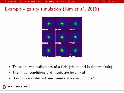
Example - Lorenz63 forward model

1000 draws from forward model for Lorenz63 system at four fixed time points.

Slide 17/29


For probabilistic numerics

If the state is deterministic but defined implicitly by a system ofdifferential equations, our uncertainty about the solution can be modelledprobabilistically,

[y1:T | u1:T , θ] ∝ ρ [y1:T − A (u1:T )]

[u1:T | θ] ∼ a probability measure representing uncertaintyin the solution given discretization of size N

[θ] ∼ π(θ).

We use the Bayesian uncertainty quantification approach to model thismiddle layer.

Slide 18/29


Computer model emulation

We interrogate the model at M regimes, θ1:M = (θ1, . . . , θM)>. Eachinterrogation is comprised of an ensemble of K output samples.

Let u1:K1:T (θ1:M) denote the ensemble of K output simulations for each ofthe regimes θ1:M .

[y1:T | u1:K1:T (θ1:M), u1:T , δ1:T , θ] ∝ ρ [y1:T − A (u1:T (θ))− δ1:T ]

[uk1:T (θm) | uk1:T , θ] ∼ N(uk1:T (θm),Λ

)k = 1, . . . ,K[

uk1:T | θ]∼ generative stochastic model

[θ, δ] ∼ π(θ, δ).

Slide 19/29


A Hierarchical model representation

Challenges of MCMC sampling from the posterior include:

• Emulation based on MK model evaluations is computationallyexpensive

• Models are evaluated at multiple spatio-temporal locations and overmultiple states

Our approach:

• Dimension reduction over the second (output) layer of thehierarchical model

• We include the dimension reduction specifications within thehierarchical model, resulting in a fully probabilistic approach

Slide 20/29


Example: Exact vs Emulation Based Inferencein a Model of Protein Dynamics

Slide 21/29


Inference for a model of protein dynamics

JAK-STAT chemical signaling pathway model describes concentration of4 STAT factors by a delay differential equation system on t ∈ [0, 60],

Illustration of the JAK-STAT mechanism

d

dtu(1)(t, θ) = −k1 u(1)(t, θ)EpoRA(t) + 2 k4 u

(4)(t − τ, θ)

d

dtu(2)(t, θ) = k1 u

(1)(t, θ)EpoRA(t)− k2(u(2)(t, θ)

)2

d

dtu(3)(t, θ) = −k3 u(3)(t, θ) + 0.5 k2

(u(2)(t, θ)

)2

d

dtu(4)(t, θ) = k3 u

(3)(t, θ)− k4 u(4)(t − τ, θ)

u(i)(t, θ) = φ(i)(t), t ∈ [−τ, 0], i = 1, . . . , 4

Slide 22/29


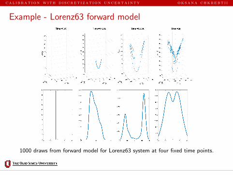
Inference for a model of protein dynamics

States are observed indirectly through a nonlinear transformation:

Experimental measurements

A(1) = k5(u(1)(t; θ) + 2u(3)(t; θ)

)A(2) = k6

(u(1)(t; θ) + u(2)(t; θ) + 2u(3)(t; θ)

)A(3) = u(1)(t; θ)

A(4) =u(3)(t; θ)

u(2)(t; θ) + u(3)(t; θ)

Observations are noisy measurements on the transformed states andforcing function at points t = {tij}i=1,...,4;j=1,...,ni

y(t) = Ak4,k5u(t; k1, . . . , k6, τ, φ,EpoRA) + ε(t)

Slide 23/29


Results: exact inference

Slide 24/29


Results: emulation based inference

●

●

●

●●

●● ●

●

●● ● ●

●

● ●

−0.5

0.5

1.0

1.5

2.0

time (minutes)0 4 8 14 20 30 40 50 60

●

●

●

●●

●● ●

●

●● ● ●

●

● ●

● y1(θ)κ1(χ2(θ) + 2χ3(θ)) + δ1

●●

● ●

●●

● ●● ●

● ●●

●

●●

−0.5

0.5

1.0

1.5

2.0

time (minutes)0 4 8 14 20 30 40 50 60

●●

● ●

●●

● ●● ●

● ●●

●

●●

● y2(θ)κ2(χ1(θ) + χ2(θ) + 2χ3(θ)) + δ2

●

●

●

●●

●● ●

●

●● ● ●

●

● ●

−0.5

0.5

1.0

1.5

2.0

time (minutes)0 4 8 14 20 30 40 50 60

●

●

●

●●

●● ●

●

●● ● ●

●

● ●

● y1(θ)δ1

●●

● ●

●●

● ●● ●

● ●●

●

●●

−0.5

0.5

1.0

1.5

2.0

time (minutes)0 4 8 14 20 30 40 50 60

●●

● ●

●●

● ●● ●

● ●●

●

●●

● y2(θ)δ2

●

●

●

●●

●● ●

●

●● ● ●

●

● ●

−0.5

0.5

1.0

1.5

2.0

time (minutes)0 4 8 14 20 30 40 50 60

●

●

●

●●

●● ●

●

●● ● ●

●

● ●

● y1(θ)κ1(χ2(θ) + 2χ3(θ))

●●

● ●

●●

● ●● ●

● ●●

●

●●

−0.5

0.5

1.0

1.5

2.0

time (minutes)0 4 8 14 20 30 40 50 60

●●

● ●

●●

● ●● ●

● ●●

●

●●

● y2(θ)κ2(χ1(θ) + χ2(θ) + 2χ3(θ))

Slide 25/29


Results: emulation based inference

0 2 4 6

0

0.5

1

θ1

0 2 4 6

0

1

2

θ2

0 0.5 1 1.5 2

0 2 4 6

0

1

2

θ3

0 0.5 1 1.5 20 0.5 1 1.5 2

0 2 4 6

0

1

2

θ4

0 0.5 1 1.5 20 0.5 1 1.5 20 0.5 1 1.5 2

0 2 4 6

0

5

θ5

0 0.5 1 1.5 20 0.5 1 1.5 20 0.5 1 1.5 20 2 4 6

0 2 4 6

100

200

300

400

θ6

0 0.5 1 1.5 20 0.5 1 1.5 20 0.5 1 1.5 20 2 4 6100 200 300 400

0 2 4 6

0

1

2

θ7

×105

0 0.5 1 1.5 20 0.5 1 1.5 20 0.5 1 1.5 20 2 4 6100 200 300 4000 0.5 1 1.5 2

×105

0 2 4 6

θ1

0

5

θ8

0 0.5 1 1.5 2

θ2

0 0.5 1 1.5 2

θ3

0 0.5 1 1.5 2

θ4

0 2 4 6

θ5

100 200 300 400

θ6

0 0.5 1 1.5 2

θ7

×105

0 2 4 6

θ8

Kernel density estimates of the marginal stochastically calibrated posterior (gray) withM = 100 model runs, and exact posterior (black) for the JAK-STAT system. Marginal prior

densities are shown as dotted lines.

Slide 26/29


Thank you!

Slide 27/29


References

1 Pratola, M.T., Chkrebtii, O.A. Bayesian Calibration of MultistateStochastic Simulators. To appear in Statistica Sinica.

2 Chkrebtii, O.A., Campbell, D.A., Calderhead, B., Girolami, M. , BayesianSolution Uncertainty Quantification for Differential Equations , BayesianAnalysis with discussion, 11(4), 1239-1267, 2016.

3 Arnold, A., Calvetti, D, Somersalo, E. Linear multistep methods, particlefiltering and sequential Monte Carlo, Inverse Problems, 29, 2013.

4 Conrad, R., Girolami, M., Sarkka, S., Stuart, A., Zygalakis, K. Statisticalanalysis of differential equations: introducing probability measures onnumerical solutions, Statistics and Computing, 2016.

5 Lie, H.C., Stuart, A. M., Sullivan, T. J. Strong convergence rates ofprobabilisti integrators for ordinary differential equations, arXiv preprint,2017.

Slide 28/29


References

1 Hennig, P., Hauberg, S. Probabilistic Solutions to Differential Equationsand their Application to Riemannian Statistics, In Proc. of the 17th int.Conf. on Artificial Intelligence and Statistics (AISTATS) (Vol. 33). JMLR,W&CP, 2014.

2 Schober, M., Duvenaud, D. K., Hennig, P. Probabilistic ODE Solvers withRunge-Kutta Means. In Z. Ghahramani, M. Welling, C. Cortes, N. D.Lawrence, & K. Q. Weinberger (Eds.), Advances in Neural InformationProcessing Systems 27 (pp. 739747). Curran Associates, Inc, 2014.

3 Skilling, J. Bayesian solution of ordinary differential equations MaximumEntropy and Bayesian Methods, Seattle, 1991.

4 Kim et al., The AGORA High-resolution Galaxy Simulations ComparisonProject, The Astrophysical Journal Supplement Series, 2014.

5 Swameye et al., Identification of nucleocytoplasmic cycling as a remotesensor in cellular signaling by databased modeling. PNAS, 2003.

Slide 29/29

Documents

@let@token Bayesian Calibration of Simulators with ... · Bayesian Calibration of Simulators with Structured Discretization Uncertainty Oksana A. Chkrebtii Department of Statistics,