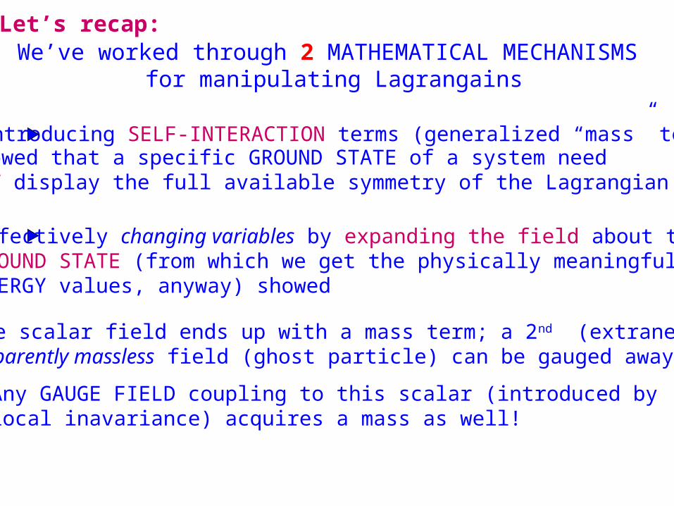
Let’s recap:We’ve worked through 2 MATHEMATICAL MECHANISMS

for manipulating Lagrangains

Introducing SELF-INTERACTION terms (generalized “mass” terms)showed that a specific GROUND STATE of a system need NOT display the full available symmetry of the Lagrangian

Effectively changing variables by expanding the field about the GROUND STATE (from which we get the physically meaningful ENERGY values, anyway) showed

•The scalar field ends up with a mass term; a 2nd (extraneous) apparently massless field (ghost particle) can be gauged away.

•Any GAUGE FIELD coupling to this scalar (introduced by local inavariance) acquires a mass as well!

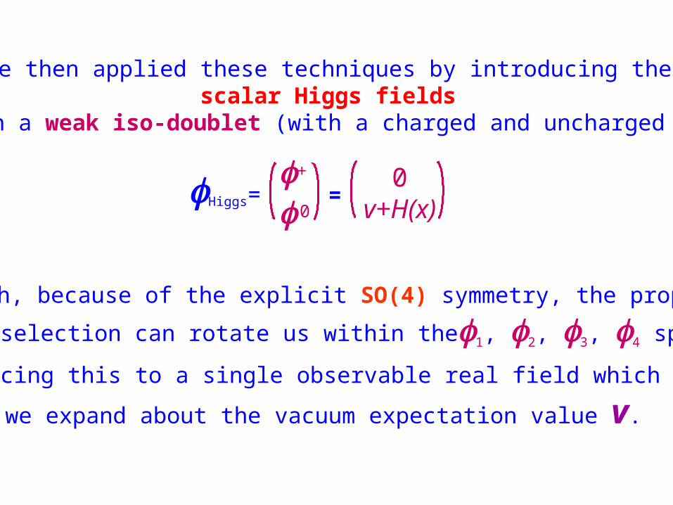
We then applied these techniques by introducing the scalar Higgs fields

through a weak iso-doublet (with a charged and uncharged state)

+

0Higgs=

0v+H(x)

=

which, because of the explicit SO(4) symmetry, the proper

gauge selection can rotate us within the1, 2, 3, 4 space,

reducing this to a single observable real field which we we expand about the vacuum expectation value v.

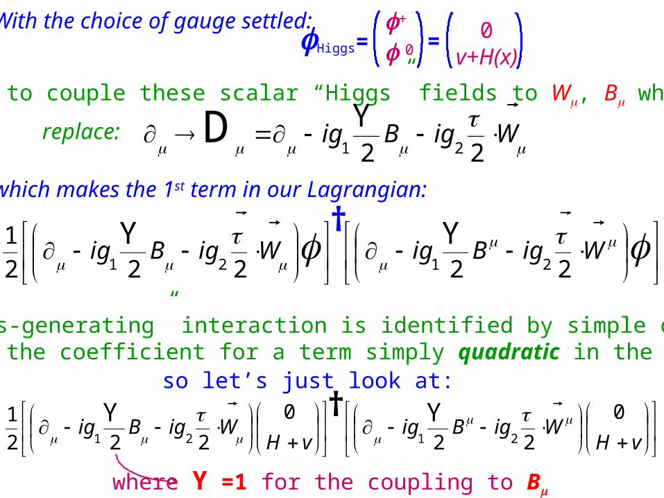
With the choice of gauge settled: +

0Higgs=0

v+H(x)=

Let’s try to couple these scalar “Higgs” fields to W, B which means

WigBig

22 21

YDreplace:

which makes the 1st term in our Lagrangian:

WigBigWigBig

22222

12121

YY †

The “mass-generating” interaction is identified by simple constantsproviding the coefficient for a term simply quadratic in the gauge fields

so let’s just look at:

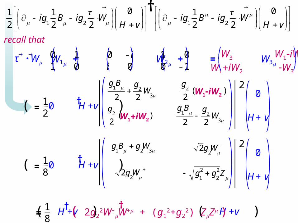
vHWigBig

vHWigBig

0

22

0

222

12121

YY †

where Y =1 for the coupling to B

vHWigBig

vHWigBig

0

22

10

22

1

2

12121

†

recall that

τ ·W→ →

= W1 + W2 + W30 11 0

0 -ii 0

1 00 -1

= W3 W1iW2

W1iW2 W3

12

= ( )

3

21

22W

gBg

2

321

22W

gBg

)(2

2 g

)(2

2 g

0

H + v0 H +v

18

= ( ) 321

WgBg 2

Zgg 2

2

2

1

Wg2

2 0

H + v0 H +v

†

†

18

= ( )H +v† ( )H +v

W1iW2

W1iW2

Wg2

2

( 2g22W+

W+ + (g12+g2

2) ZZ )†

18

= ( )H +v† ( )H +v( 2g22W+

W+ + (g12+g2

2) ZZ )†

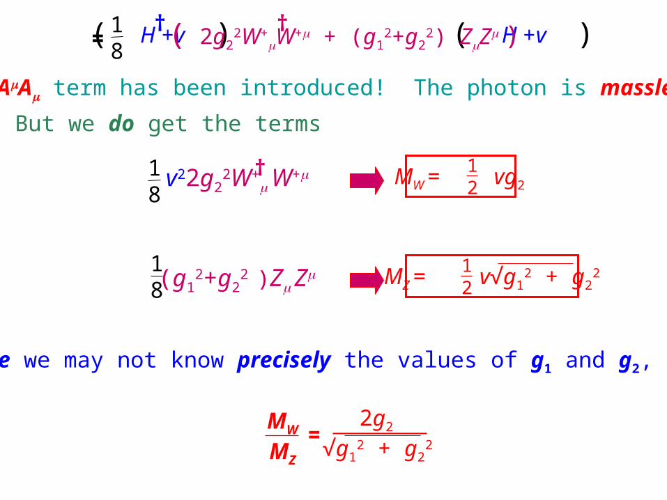
No AA term has been introduced! The photon is massless!

But we do get the terms

18

v22g22W+

W+† MW = vg2

18 (g1

2+g22 )Z Z MZ = v√g1

2 + g221

2

MW

MZ

2g2

√g12 + g2

2

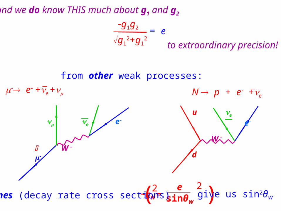
At this stage we may not know precisely the values of g1 and g2, but note:

=

12

e e

W

u e

e

W

d

e+e + N p + e+e

~gW =e

sinθW( )2 2

g1g2

g12+g1

2 = e

and we do know THIS much about g1 and g2

to extraordinary precision!

from other weak processes:

lifetimes (decay rate cross sections) give us sin2θW

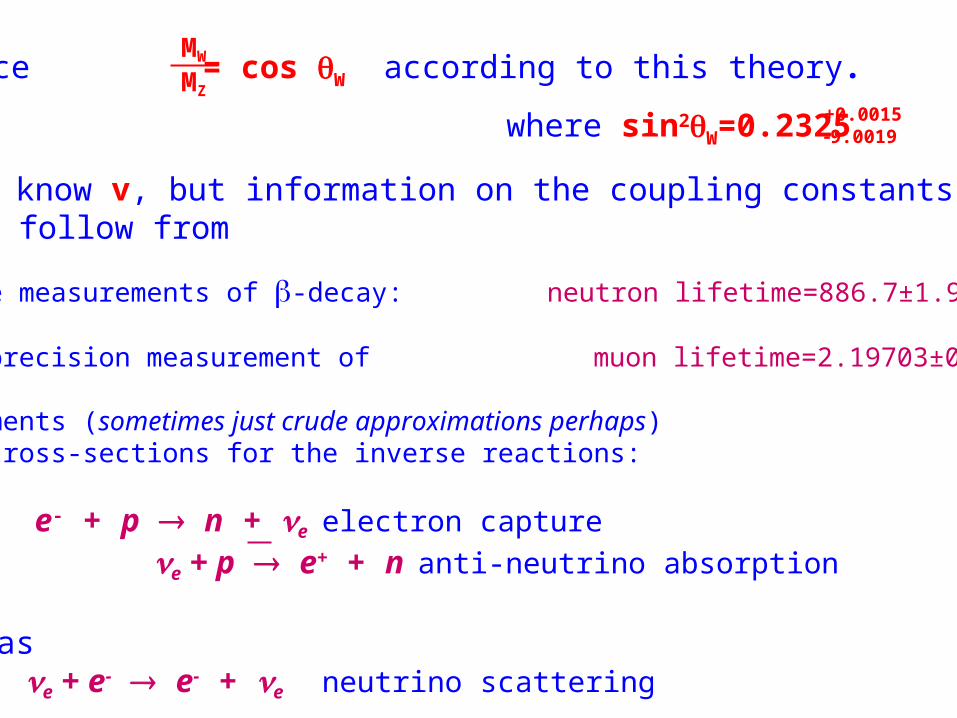
Notice = cos W according to this theory.MW

MZ

where sin2W=0.2325 +0.00159.0019

We don’t know v, but information on the coupling constants g1 and g2 follow from

• lifetime measurements of -decay: neutron lifetime=886.7±1.9 sec and • a high precision measurement of muon lifetime=2.19703±0.00004 sec and • measurements (sometimes just crude approximations perhaps) of the cross-sections for the inverse reactions:

e- + p n + eelectron capture

e + p e+ + n anti-neutrino absorption

as well as e + e- e- + e neutrino scattering

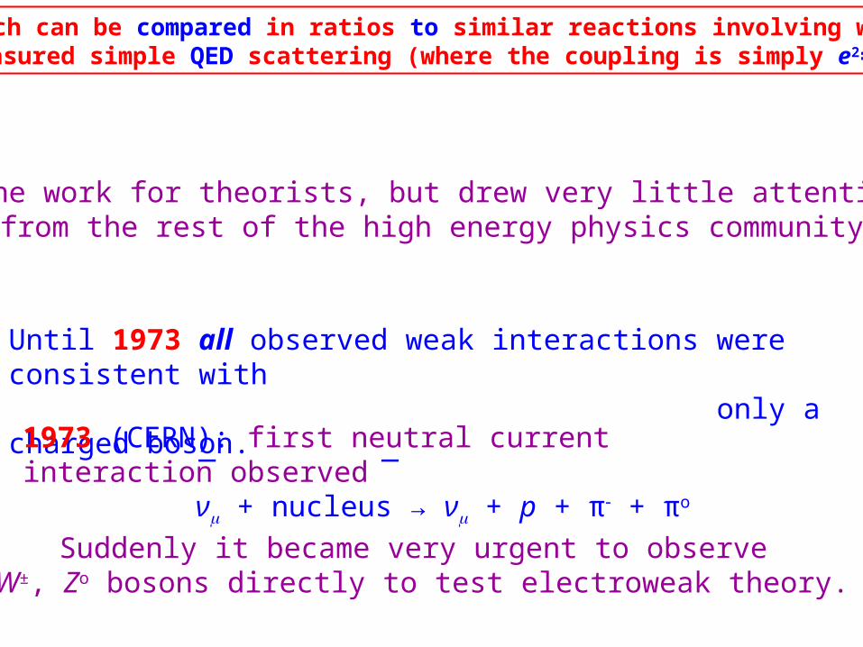
Until 1973 all observed weak interactions were consistent with only a charged boson.

All of which can be compared in ratios to similar reactions involving well-known/well-measured simple QED scattering (where the coupling is simply e2=1/137).

Fine work for theorists, but drew very little attentionfrom the rest of the high energy physics community

1973 (CERN): first neutral current interaction observed ν + nucleus → ν + p + π + πo

Suddenly it became very urgent to observe W±, Zo bosons directly to test electroweak theory.

_ _

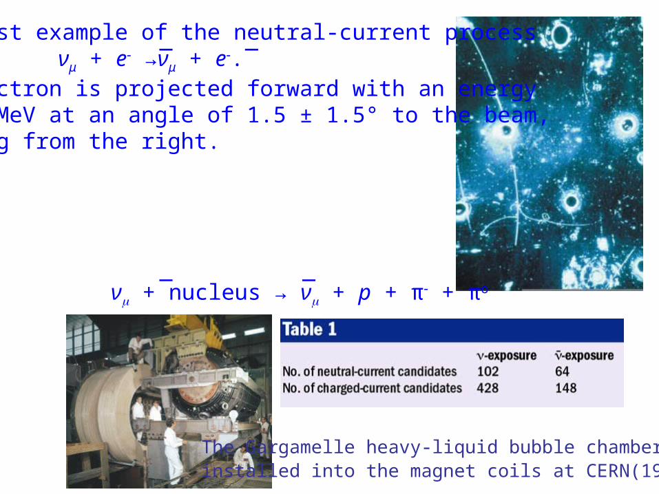
The Gargamelle heavy-liquid bubble chamber, installed into the magnet coils at CERN(1970)

The first example of the neutral-current process νμ + e →νμ + e. The electron is projected forward with an energy of 400 MeV at an angle of 1.5 ± 1.5° to the beam, entering from the right.

ν + nucleus → ν + p + π + πo

__

_ _

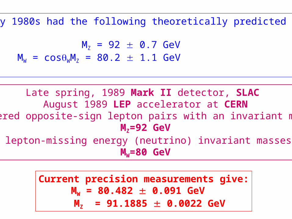
By early 1980s had the following theoretically predicted masses:

MZ = 92 0.7 GeV MW = cosWMZ = 80.2 1.1 GeV

Late spring, 1989 Mark II detector, SLAC August 1989 LEP accelerator at CERN

discovered opposite-sign lepton pairs with an invariant mass ofMZ=92 GeV

and lepton-missing energy (neutrino) invariant masses ofMW=80 GeV

Current precision measurements give: MW = 80.482 0.091 GeV MZ = 91.1885 0.0022 GeV

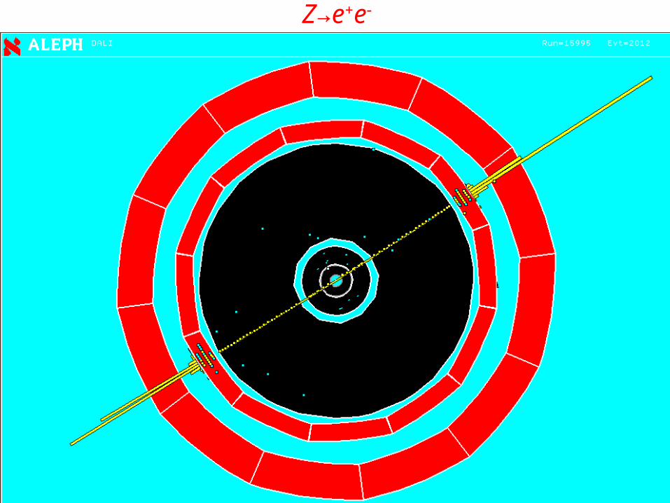
Z→e+e

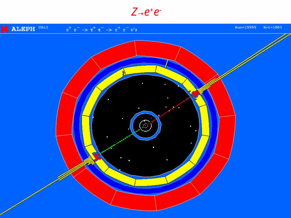
Z→e+e

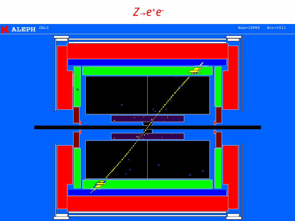
Z→e+e

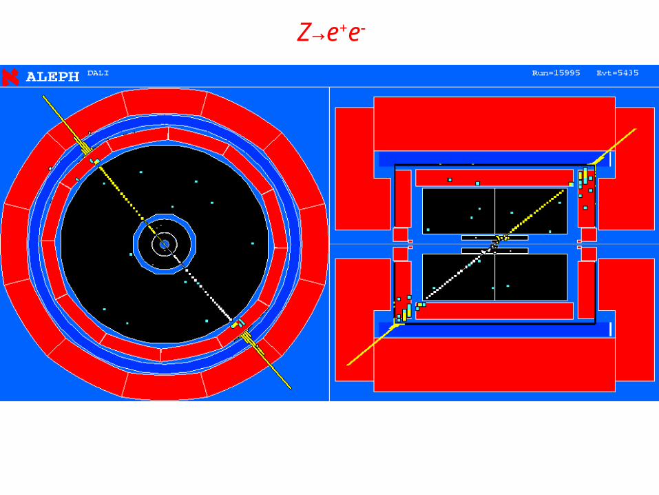
Z→e+e

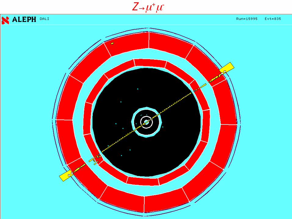
Z→+

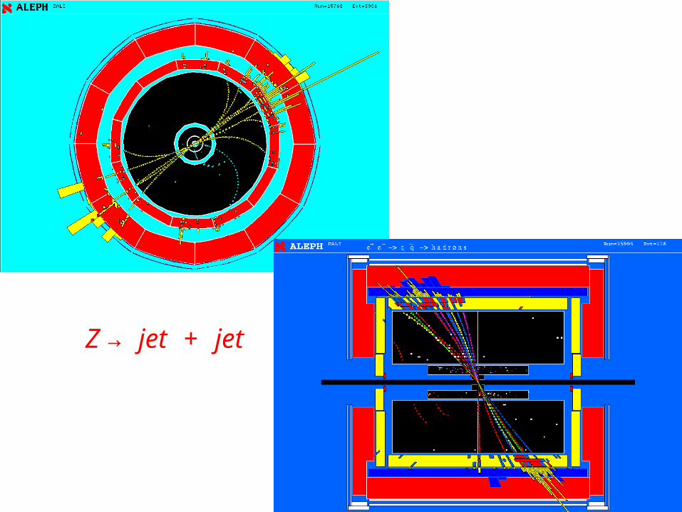
Z → jet + jet

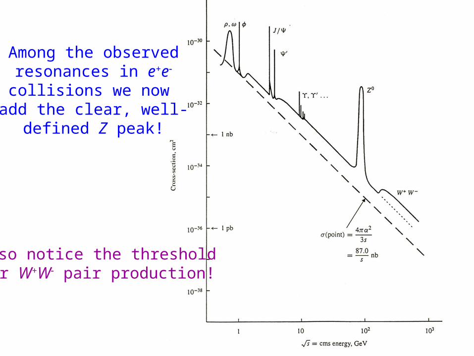
Among the observedresonances in e+e

collisions we now add the clear, well-

defined Z peak!

Also notice the thresholdfor W+W pair production!

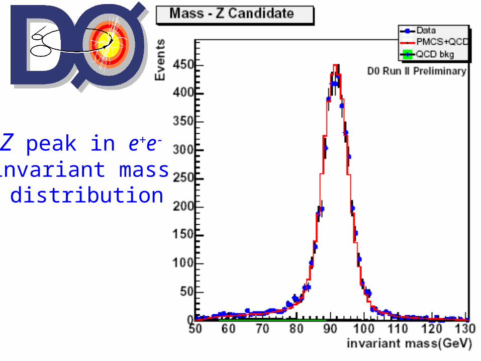
Z peak in e+e invariant mass

distribution

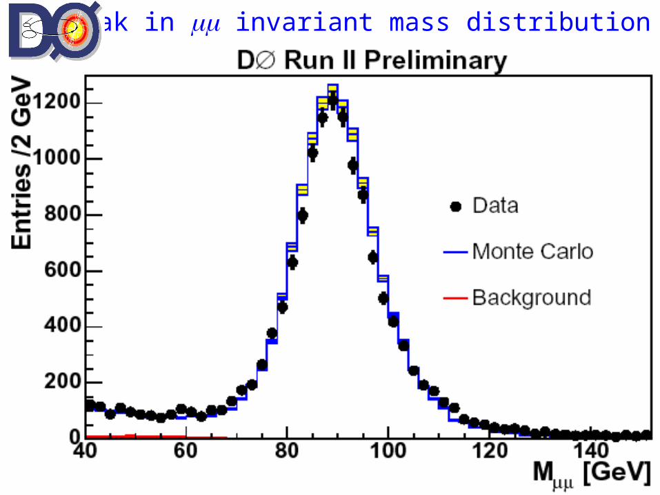
Z peak in invariant mass distribution

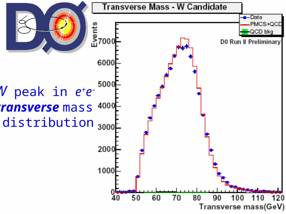
W peak in e+e transverse mass

distribution

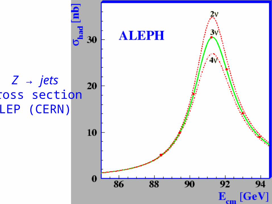
Z → jetscross sectionLEP (CERN)

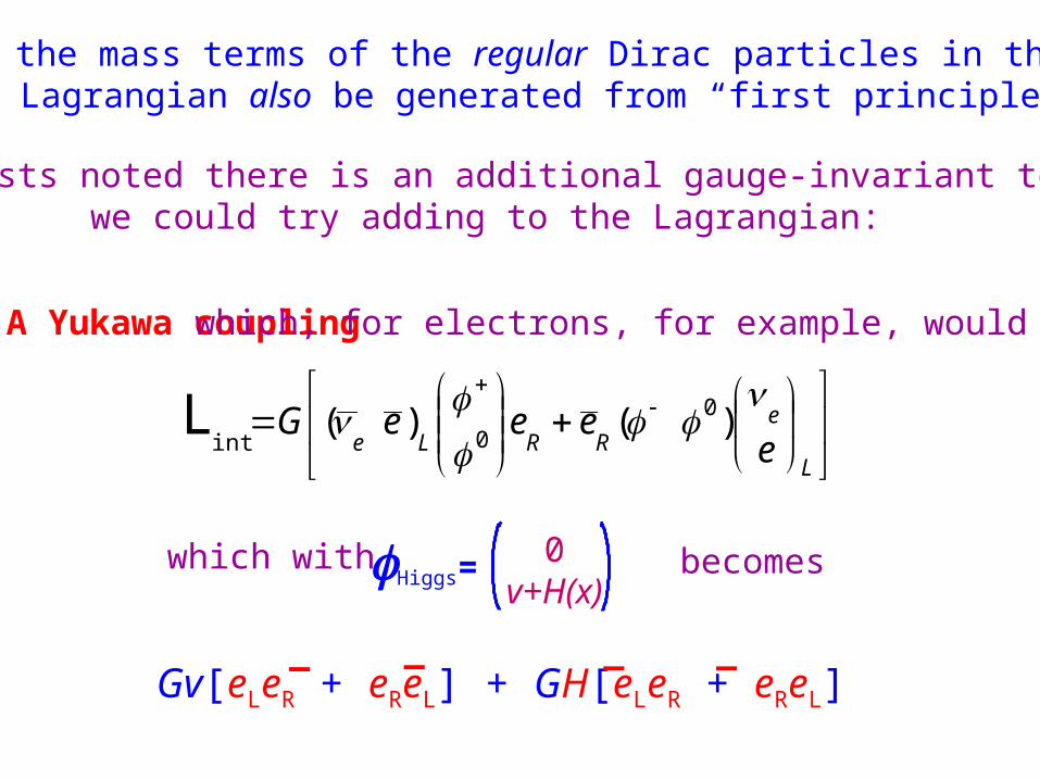
Can the mass terms of the regular Dirac particles in theDirac Lagrangian also be generated from “first principles”?

Theorists noted there is an additional gauge-invariant termwe could try adding to the Lagrangian:

A Yukawa coupling which, for electrons, for example, would read

L

eRRLe e

eeeG

)()( 0

0int L

which with Higgs=0

v+H(x)becomes

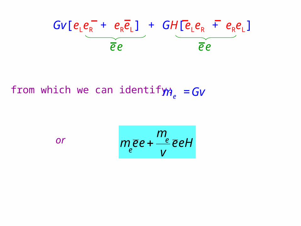
Gv[eLeR + eReL] + GH[eLeR + eReL] _ _ _ _

e e_

e e_

from which we can identify: me = Gv

or eHev

meem e

e

Gv[eLeR + eReL] + GH[eLeR + eReL] _ _ _ _