Lessons learnt from a deep excavation for future …eprints.whiterose.ac.uk/125771/15/Lessons learnt from a...Full Length Article Lessons learnt from a deep excavation for future application

lable at ScienceDirect

Journal of Rock Mechanics and Geotechnical Engineering 10 (2018) 468e485

Contents lists avai

Journal of Rock Mechanics andGeotechnical Engineering

journal homepage: www.rockgeotech.org

Full Length Article

Lessons learnt from a deep excavation for future application of theobservational method

Raul Fuentes a,*, Anton Pillai b, Pedro Ferreira c

a School of Civil Engineering, University of Leeds, Leeds, LS2 9JT, UKbOve Arup and Partners, 13 Fitzroy Street, London, W1T 4BQ, UKcDepartment of Civil, Environmental & Geomatic Engineering, University College London, Chadwick Building, Gower Street, London, WC1E 6BT, UK

a r t i c l e i n f o

Article history:Received 30 August 2017Received in revised form7 December 2017Accepted 13 December 2017Available online 21 March 2018

Keywords:Deep excavationBasementGround movementsWall movementsRetaining wallCorner effectsTime-dependent movements

* Corresponding author.E-mail addresses: [email protected] (R. Fue

(A. Pillai), [email protected] (P. Ferreira).Peer review under responsibility of Institute of R

nese Academy of Sciences.

https://doi.org/10.1016/j.jrmge.2017.12.0041674-7755 � 2018 Institute of Rock and Soil MechanicNC-ND license (http://creativecommons.org/licenses/

a b s t r a c t

This paper draws lessons learnt from a comprehensive case study in overconsolidated clay. Apart fromthe introduction of the case study, including field measurements, the paper draws on the observationsand a three-dimensional (3D) numerical analysis to discuss the implications of observations in theapplication of the observational method (OM) in the context of the requirements of EUROCODE 7 (EC7).In particular, we focus on corner effects and time-dependent movements and provide initial guidance onhow these could be considered. Additionally, we present the validation of a new set of parameters tocheck that it provides a satisfactory compliance with EC7 as a set of design parameters. All these findingsand recommendations are particularly important for those who want to use the OM in similar futureprojects.� 2018 Institute of Rock and Soil Mechanics, Chinese Academy of Sciences. Production and hosting byElsevier B.V. This is an open access article under the CC BY-NC-ND license (http://creativecommons.org/

licenses/by-nc-nd/4.0/).

1. Introduction

As a design and construction framework, the observationalmethod (OM) was introduced by Peck (1969) and has since seenmany applications over the years (e.g. Glass and Powderham, 1994;Powderham, 1994, 2002; Powderham and Rutty, 1994; Peck, 2001;Sakurai et al., 2003; Chapman and Green, 2004; Finno and Calvello,2005; Yeow and Feltham, 2008; Nicholson et al., 2014; Spross andJohansson, 2017).

OM can be approached in multiple forms. However, within thecontext of this paper, we focus on the philosophy of EUROCODE 7(EC7) Clause 2.7 (British Standards Institute, 2004) to provide aframework for our discussion against an established design stan-dard. EC7 states the following requirements for the application ofthe OM before construction starts:

(1) Acceptable limits of behaviour shall be established.

ntes), [email protected]

ock and Soil Mechanics, Chi-

s, Chinese Academy of Sciences. Prby-nc-nd/4.0/).

(2) The range of possible behaviour shall be assessed and it shall beshown that there is an acceptable probability that the actualbehaviour will be within the acceptable limits.

(3) A plan of monitoring shall be devised, which will reveal whetherthe actual behaviour lies within the acceptable limits. The moni-toring shall make this clear at a sufficiently early stage, and withsufficiently short intervals to allow contingency actions to be un-dertaken successfully.

(4) The response time of the instruments and the procedures foranalysing the results shall be sufficiently rapid in relation to thepossible evolution of the system.

(5) A plan of contingency actions shall be devised, which may beadopted if the monitoring reveals behaviour outside acceptablelimits.

In particular, we will provide a commentary of the observedbehaviour of a deep excavation and its impact on the first four EC7requirements as shown above. A methodology of how to set thetrigger values or a set of action plans is not covered in this articlebut is thoroughly presented by Spross and Johansson (2017). In thispaper, the focus is on the behaviour that may affect the generalapplication of OM in relation to the above requirements.

oduction and hosting by Elsevier B.V. This is an open access article under the CC BY-

http://creativecommons.org/licenses/by-nc-nd/4.0/


mailto:[email protected]



http://crossmark.crossref.org/dialog/?doi=10.1016/j.jrmge.2017.12.004&domain=pdf

www.sciencedirect.com/science/journal/16747755

http://www.rockgeotech.org

https://doi.org/10.1016/j.jrmge.2017.12.004




R. Fuentes et al. / Journal of Rock Mechanics and Geotechnical Engineering 10 (2018) 468e485 469

The commentary includes some initial guidance on how to over-come this behaviour for the future application of OM in similarconditions.

The complexity of current deep excavations, due to the con-gested urban environments, means that sophisticated analyses areneeded to satisfy the requirements of all stakeholders involved inthese projects which, in cities, also include the third-party neigh-bours. These analyses are typically three-dimensional (3D) nu-merical models that require adequate constitutive relationships tocharacterise soil behaviour. In the case covered in this paper, wefocus on the use of the BRICK soil model (Simpson,1992), which hasbeen validated for characteristic parameters (defined in the nextsection) and provides adequate design parameters for deep exca-vations in undrained London Clay (Ng et al., 1998; Long, 2001; Yeowet al., 2006).

To date, however, a validation of most probable (also defined inthe next section) BRICK soil model parameters has not yet beencarried out and it is a necessity for future applications of the OMusing BRICK soil model. Furthermore, it is known that excavationspresent 3D effects, particularly around their corners, as well astime-dependent effects that need to be considered when settingthe trigger values. This is particularly necessary to avoid situationswhere measured movements exceed those triggers. Therefore, thispaper has three main objectives:

(1) Validate a set of most probable parameters for BRICK soilmodel in 3D, using undrained analysis for a case study inLondon Clay; given that in conjunction with the alreadyvalidated characteristic parameters, it can provide a suffi-cient range of behaviours for the application of OM.

(2) Observe the corner effects of the case study in relation toproviding guidance of how these can be considered withinthe operation of OM.

(3) Observe the time-dependent movements and provide guid-ance of how these could be included in the predictionswithin the operation of OM.

2. Observational method e design parameters

The EC7 requirements presented above are very broad and havebeen approached in multiple ways by different authors. Of partic-ular interest are theworks (Prästings et al., 2014; Spross et al., 2016)applied to other types of geotechnical structures. In the context, thefocus is on the design parameters and the behaviour of theretaining wall, following the recommendations of Nicholson et al.(1999). EC7 requirements 1 and 2 of the list above are related tothe definition of a range of behaviours. Nicholson et al. (1999)recommended the use of two sets of design parameters to dothis: ‘most probable’ and ‘characteristic’. The former, with suchname introduced by Powderham (1994) and Nicholson et al. (1999),defined it as: “a set of parameters that represent the probabilisticmean of all possible set of conditions. It represents, in generalterms, the design condition most likely to occur in practise”. Asother authors have done in the past (e.g. Yeow and Feltham, 2008;Nicholson et al., 2014), we define them as those parameters thatprovide the closest response to reality in terms of displacements(i.e. monitoring data). The second set agrees with the terminologyused in EC7 (British Standards Institute, 2004) and is defined as: acautious estimate of the value affecting the occurrence of the limitstate. Hence, both sets of parameters differ in their degree ofcautiousness with the ‘characteristic’ being a more cautious set ofparameters. Both sets allow the prediction of two separate triggervalues that give a range to dictate when actions are required (i.e.point 5 of the EC7 requirements). In order to fulfil EC7 requirements

3 and 4, both sets also need to provide a range of behaviours thatcan be easily differentiated and also monitored timely. For this,Nicholson et al. (1999) recommended that both sets of parametersare validated against real case studies using similar sites, which iswhat this paper provides for deep excavations.

3. Site description

3.1. Site and existing structures

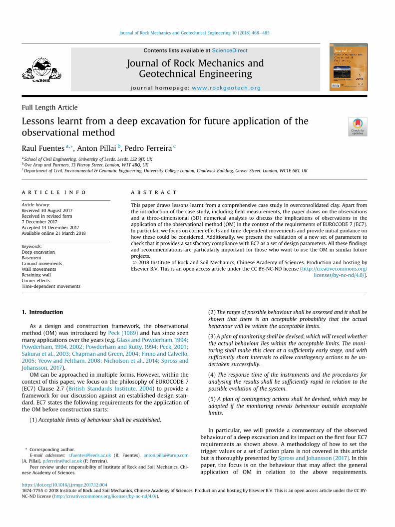
The site is located in the vicinity of Aldgate Station in London,UK. The site is bounded to the southeast by St. Botolph Street, to thesouthwest by Houndsditch, and to the northwest by Stoney Lane(Fig. 1). White Kennett Street forms the northern site boundarywith the London Underground (LUL) District andMetropolitan linesrunning along the eastern site boundary through a cut and covertunnel. The site dimensions are approximately 90 m � 65 m(length � width). Ground level around the site rises fromapproximately þ14 mOD to þ15.5 mOD in the north/south direc-tion, where mOD stands for metres above Ordnance Datum.

The site was occupied, before the project started, by twobuildings: St. Botolph’s House and Ambassador House as shown inFig. 1. St. Botolph’s House was designed and built in the 1960s. Itwas an 8-storey concrete frame building on pad foundations with asingle basement; the basement occupied most of the site footprintand its level was typically at þ11.0 mOD. Ambassador House wasbuilt in the 1980s and occupied the northern part of the site. It wasa 12-storey concrete frame building with a single basement foun-ded on a raft. The basement was used as a car park with a rampedaccess off St. Botolph Street, parallel to an LUL tunnel (Fig. 2). Thebasement level was typically at þ10.5 mOD.

3.2. Adjacent structures

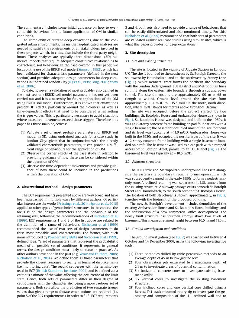
The LUL Circle and Metropolitan underground lines run along-side the eastern site boundary through a former open cut, whichwas subsequently capped in the early 1990s to form a pedestrians-only zone. A reclined retaining wall separates the LUL tunnels fromthe existing structure. A subway passage exists beneath St. BotolphStreet and Houndsditch, to the south corner of St. Botolph’s House.The location of both structures is shown, approximately, in Fig. 2,together with the footprint of the proposed building.

The new St. Botolph’s development includes demolition of theexisting Ambassador House and St. Botolph’s House buildings andthe construction of a new commercial office development. Thenewly built structure has fourteen storeys above two levels ofbasement. This means a retained height between 10.5 m and 11.5 m.

3.3. Ground investigation and conditions

The ground investigation (see Fig. 2) was carried out between 4October and 14 December 2006, using the following investigativetools:

(1) Three boreholes drilled by cable percussive methods to anaverage depth of 45 m below ground level;

(2) Four observation pits excavated to a maximum depth of2.1 m to investigate areas of potential contamination;

(3) Six horizontal concrete cores to investigate existing base-ment walls;

(4) Six vertical cores to investigate the existing basementstructure;

(5) Four inclined cores and one vertical core drilled using aBeretta T41 track mounted rotary rig to investigate the ge-ometry and composition of the LUL reclined wall and to

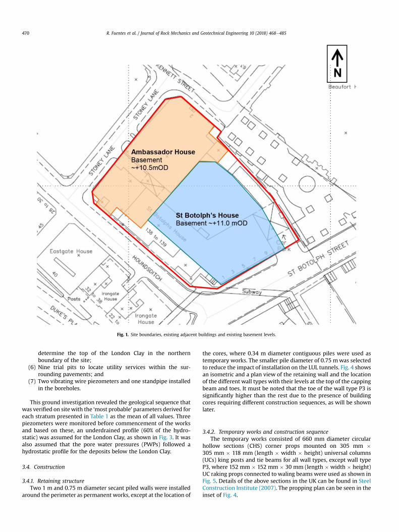
Fig. 1. Site boundaries, existing adjacent buildings and existing basement levels.

R. Fuentes et al. / Journal of Rock Mechanics and Geotechnical Engineering 10 (2018) 468e485470

determine the top of the London Clay in the northernboundary of the site;

(6) Nine trial pits to locate utility services within the sur-rounding pavements; and

(7) Two vibrating wire piezometers and one standpipe installedin the boreholes.

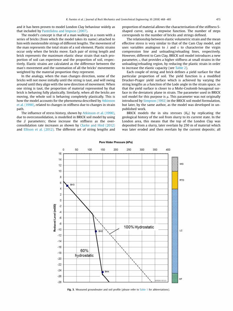
This ground investigation revealed the geological sequence thatwas verified on sitewith the ‘most probable’ parameters derived foreach stratum presented in Table 1 as the mean of all values. Threepiezometers were monitored before commencement of the worksand based on these, an underdrained profile (60% of the hydro-static) was assumed for the London Clay, as shown in Fig. 3. It wasalso assumed that the pore water pressures (PWPs) followed ahydrostatic profile for the deposits below the London Clay.

3.4. Construction

3.4.1. Retaining structureTwo 1 m and 0.75 m diameter secant piled walls were installed

around the perimeter as permanent works, except at the location of

the cores, where 0.34 m diameter contiguous piles were used astemporary works. The smaller pile diameter of 0.75 mwas selectedto reduce the impact of installation on the LUL tunnels. Fig. 4 showsan isometric and a plan view of the retaining wall and the locationof the different wall types with their levels at the top of the cappingbeam and toes. It must be noted that the toe of the wall type P3 issignificantly higher than the rest due to the presence of buildingcores requiring different construction sequences, as will be shownlater.

3.4.2. Temporary works and construction sequenceThe temporary works consisted of 660 mm diameter circular

hollow sections (CHS) corner props mounted on 305 mm �305 mm � 118 mm (length � width � height) universal columns(UCs) king posts and tie beams for all wall types, except wall typeP3, where 152 mm � 152 mm � 30 mm (length � width � height)UC raking props connected to waling beams were used as shown inFig. 5. Details of the above sections in the UK can be found in SteelConstruction Institute (2007). The propping plan can be seen in theinset of Fig. 4.

Fig. 2. Location of the ground investigation points, LUL tunnel and subway locations.

Table 1Soil stratigraphy and ‘most probable’ parameters obtained from site investigation.

Soil type Top of strata(mOD)

g (kN/m3) E0

(MPa)n 40 (�) K0

Made ground (MG) þ15.5 - þ14.5 18 1 0.2 25 0.58River terrace deposits (RTD) þ10.2 20 3.5 0.2 35 0.43London Clay (LC) þ4.2 20 BRICK soil modele see

Table 2Harwich formation (HF) �27.5 20 150 0.2 39 0.37Thanet sand (TS) �45 20 150 0.2 39 0.37

Note: g represents the bulk density, E0 is the drained Young’s modulus, n is thePoisson’s ratio, 40 is the angle of shear resistance, and K0 is the earth pressure co-efficient at rest.

Table 2BRICK soil model parameters.

Parameter ‘Characteristic’ ‘Most probable’

l 0.1 0.1k 0.02 0.02i 0.0019 0.00175n 0.2 0.2m 1.3 1.3bG, bf 4 4

Gt/Gmax

(strain)String lengths (shear strain)

‘Characteristic’ ‘Most probable’

0.92 3.04 � 10�5 3 � 10�5

0.75 6.08 � 10�5 7.5 � 10�5

0.53 1.01 � 10�4 1.5 � 10�4

0.29 1.21 � 10�4 4 � 10�4

0.13 8.2 � 10�4 7.5 � 10�4

0.075 1.71 � 10�3 1.5 � 10�3

0.044 3.52 � 10�3 2.5 � 10�3

0.017 9.69 � 10�3 7.5 � 10�3

0.0035 2.22 � 10�2 2 � 10�2


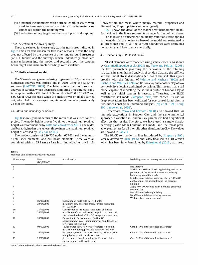
A bottom-up excavation sequence was adopted, as shown inFig. 6. The figure contains snapshots at key construction dates,starting on 5 March 2008. Prior to this date, the existing build-ings were demolished, the basement was backfilled tolevel þ14.65 mOD, and the piles were installed for the secantpiled wall. Table 3 provides a description of the main construc-tion activities in the middle column. The modelled constructionsequence in the right-hand side is based on the ‘as built’ recordsand focussing on the north-west corner. Further details areprovided in Section 4.4.

0 6.46 � 10�2 6 � 10�2

Note: Gmax is the maximum shear modulus, Gt is the shear modulus at a given strainlevel, l is the slope of the isotropic normal compression line and k is the slope of theisotropic swelling line in evol - ln p0 space, i is a parameter controlling elastic stiff-ness, m controls string length due to changes in orientation in the p-plane, bG and bfcontrol the amount of initial stiffness and strength gain from overconsolidation. Allparameters do not have units, except the shear moduli.

3.5. Monitoring system

3.5.1. Installed systemA comprehensive monitoring scheme was implemented on site

(see Fig. 7), which consisted of:

(1) 37 precise levelling studs on surrounding pavements, sub-ways, footpaths and structures.

(2) 14 reflective survey targets on adjacent buildings.(3) 4 tiltmeters and 4 reflective survey targets for the LUL tunnel

retaining wall.


(4) 8 manual inclinometers with a probe length of 0.5 m wereused to take measurements within an inclinometer caseembedded within the retaining wall.

(5) 8 reflective survey targets on the secant piled wall capping.

3.5.2. Selection of the area of studyThe area selected for close study was the north area indicated in

Fig. 7. This area was chosen for two main reasons: it was the onlyarea not affected by the presence of other underground structures(i.e. LUL tunnels and the subway), which undoubtedly introducedmany unknowns into the model, and secondly, both the cappingbeam target and inclinometer readings were available.

4. 3D finite element model

The 3Dmeshwas generated using Hypermesh v.10, whereas thenumerical analysis was carried out in 2010, using the LS-DYNAsoftware (LS-DYNA, 2008). The latter allows for multiprocessoranalysis in parallel, which decreases computing times dramatically.A computer with a CPU Intel � Xenon � X5482 @ 3.20 GHZ and8.00 GB of RAM was used when the analysis was originally carriedout, which led to an average computational time of approximately25 min per stage.

4.1. Mesh and boundary conditions

Fig. 8 shows general details of the mesh that was used for thisproject. The model height is over five times the maximum retainedheight, as recommended by Potts and Zdravkovic (2001). Thewidthand breadth, in plan, are at least three times themaximum retainedheight as advised by Lin et al. (2003).

The model consists of 629,770 nodes, 607,634 solid elements,41,286 shell elements, and 269 beam elements. These were allcontained within 165 Parts (a Part is an individual entity in LS-

Table 3Modelled and actual construction sequence.

Model stage Date(DD/MM/YY)

Actual works

12

3

4

5678 05/03/2008 Excavation of north side to þ11.8 mO9 23/04/2008 Install first row of corner props. Furth

to þ7.9 mOD10 21/05/2008 Construction of the access ramp nort11 26/06/2008 Installation of a second row of props

site reduced to level þ7.9 mOD excep12 28/07/2008 Excavation to formation level (þ4.0 m

approximately), access ramp removatower cranes being built

13 03/09/2008 Tower cranes in place. North core staInstallation of raking props and mini

14 16/09/2008 Further progress on raft constructionminipiles location in north-west wall

15 29/09/2008 Access ramp reduced even further. Rcorner prop in north-west corner

Note: * The total core load was assumed to be 620 kPa.

DYNA within the mesh where mainly material properties anddimensions, if appropriate, can be assigned).

Fig. 9 shows the detail of the model near inclinometer Inc 06.Each colour in the figure represents a single Part as defined above.

The following displacement boundary conditions were appliedto the model: (a) the horizontal base of the model was restrained inall directions; and (b) all the vertical boundaries were restrainedhorizontally and free to move vertically.

4.2. London ClayeBRICK soil model

All soil elements were modelled using solid elements. As shownby Grammatikopoulou et al. (2008) and Yeow and Feltham (2008),the two parameters governing the behaviour of the retainingstructure, in an undrained analysis of London Clay, are the stiffnessand the initial stress distribution (i.e. K0) of the soil. This agreesbroadly with the findings of Whittle and Hashash (1992) andHashash andWhittle (1996) on Boston clay and another clay of lowpermeability showing undrained behaviour. This means that a soilmodel capable of modelling the stiffness profile of London Clay aswell as the initial stresses is necessary. Therefore, the BRICKconstitutive soil model (Simpson, 1992) was chosen; its use fordeep excavations has been validated for overconsolidated clays intwo-dimensional (2D) undrained analyses (Ng et al., 1998; Long,2001; Yeow et al., 2006).

Furthermore, Yeow and Feltham (2008) also showed that formultiple excavations in London Clay and the same numericalapproach, a variation in London Clay parameters had a significanteffect on the results. Therefore, we have used a simple elastic-perfectly plastic Mohr-Coulomb soil model and the ‘most prob-able’ parameters for all the soils other than London Clay. The valuesare showed in Table 1.

The BRICK soil model, as first introduced by Simpson (1992),later reviewed by Pillai (1996) and lastly finalised in a 3D versionwhich has been fully formulated by Ellison et al. (2012), was used,

Modelling construction sequence - additional notes

InitialisationWish in place LUL wall, existing building wall on theperimeter of the excavation zone and existingbuildings ground floor slabInstallation of existing basement slab at 10.2 mOD,application of the spread load of the previousbuildingApply new PWP profile using a drained profile forLondon ClayDemolition of existing buildingBackfill materials into existing basementWish in place new secant wall

Der excavation

h of the sitein the corner. Allt the access rampOD

l. Foundations for

rts to be built.piles. Raft cast

Core 2 - 10% of the core load is assumed*

up to half way into Core 2 - 25% of the core load is assumed*

emoval of first Core 2 - 75% of the core load is assumed*


and it has been proven to model London Clay behaviour widely asthat included by Pantelidou and Impson (2007).

The model’s concept is that of a man walking in a room with aseries of bricks (from which the model takes its name) attached tohimwith inextensible strings of different lengths. Themovement ofthe man represents the total strain of a soil element. Plastic strainsoccur only when the bricks move. Each pair of string length andbrick represents the maximum elastic shear strain that each pro-portion of soil can experience and the proportion of soil, respec-tively. Elastic strains are calculated as the difference between theman’s movement and the summation of all the bricks’ movementsweighted by the material proportion they represent.

In the analogy, when the man changes direction, some of thebricks will not move initially until the string is taut, and will swingaround until they alignwith the new direction of movement. Whenone string is taut, the proportion of material represented by thatbrick is behaving fully plastically. Similarly, when all the bricks aremoving, the whole soil is behaving completely plastically. This ishow the model accounts for the phenomena described by Atkinsonet al. (1990), related to changes in stiffness due to changes in strainpath.

The influence of stress history, shown by Atkinson et al. (1990),due to overconsolidation, is modelled in BRICK soil model by usingthe b parameters; these increase the stiffness as the over-consolidation rate increases as shown by Clarke and Hird (2012)and Ellison et al. (2012). The different set of string lengths and

Fig. 3. Measured groundwater and soil profile

proportion of material allows the characterisation of the stiffness S-shaped curve, using a stepwise function. The number of stepscorresponds to the number of bricks and strings defined.

The relationship between elastic volumetric strain and themeaneffective stress is very similar to that of the Cam Clay model, anduses variables analogous to l and k to characterise the virgincompression line and unloading/reloading lines, respectively.However, different to Cam Clay, BRICK soil model introduces a newparameter, i, that provides a higher stiffness at small strains in theunloading/reloading region, by reducing the plastic strain in orderto increase the elastic capacity (see Table 2).

Each couple of string and brick defines a yield surface for thatparticular proportion of soil. The yield function is a modifiedDrucker-Prager yield surface which is achieved by varying thestring lengths as a function of the Lode angle in the strain space, sothat the yield surface is closer to a Mohr-Coulomb hexagonal sur-face in the deviatoric plane in strain. The parameter used in BRICKsoil model for this purpose is m. This parameter was not originallyintroduced by Simpson (1992) in the BRICK soil model formulation,but later, by the same author, as the model was developed in un-published work.

BRICK models the in situ stresses (K0) by replicating thegeological history of the soil from slurry to its current state. In theLondon area, this means that the top of the London Clay wasdeposited from a slurry, later overlain by 250 m of material whichwas later eroded and then overlain by the current deposits; all

(please refer to Table 1 for abbreviations).

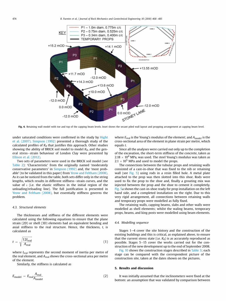
Fig. 4. Retaining wall model with toe and top of the capping beam levels. Inset shows the secant piled wall layout and propping arrangement at capping beam level.


under saturated conditions were confirmed in the study by Hightet al. (2007). Simpson (1992) presented a thorough study of thecalculated profiles of K0 that justifies this approach. Other studiesshowing the ability of BRICK soil model to model K0, and the gen-eral stressestrain behaviour of London Clay were presented byEllison et al. (2012).

Two sets of parameters were used in the BRICK soil model (seeTable 2): ‘Characteristic’ from the originally named ‘moderatelyconservative parameters’ in Simpson (1992) and, the ‘most prob-able’ (to be validated in this paper) from Yeow and Feltham (2008).As it can be noticed from the table, both sets differ only in the stringlengths, which results in different stiffnessestrain curves, and thevalue of i (i.e. the elastic stiffness in the initial region of theunloading/reloading line). The full justification is presented inYeow and Feltham (2008), but essentially stiffness governs theproblem.

4.3. Structural elements

The thicknesses and stiffness of the different elements werecalculated using the following equations to ensure that the planestrain (2D) or shell (3D) elements had an equivalent bending andaxial stiffness to the real structure. Hence, the thickness, t, iscalculated as

t ¼ffiffiffiffiffiffiffiffiffiffiffiffiffiffi12IrealAreal

s(1)

where Ireal represents the second moment of inertia per metre ofthe real element, and Areal shows the cross-sectional area per metreof the element.

Similarly, the stiffness is calculated as

Emodel ¼ ErealArealAmodel

(2)

where Ereal is the Young’s modulus of the element; and Amodel is thecross-sectional area of the element in plane strain per metre, whichequals t.

Since all the analyses were carried out only up to the completionof the excavation, the short-term stiffness of the concrete, taken as2.18 � 104 MPa, was used. The steel Young’s modulus was taken as2.1 � 105 MPa and used to model the props.

The connections between the tubular props and retaining wallsconsisted of a cast-in-shoe that was fixed to the nib or retainingwall (see Fig. 5) using rods in a resin filled hole. A metal plateattached to the prop was then slotted into this shoe. Rods wereused to fix the prop to the shoe and, finally a grouting mix wasinjected between the prop and the shoe to cement it completely.Fig. 5a shows the cast-in-shoe ready for prop installation on the lefthand side, and a completed installation on the right. Due to thisvery rigid arrangement, all connections between retaining wallsand temporary props were modelled as fully fixed.

The retaining walls, capping beams, slabs and other walls weremodelled as shell elements; whilst the waling beams, temporaryprops, beams, and king posts were modelled using beam elements.

4.4. Modelling sequence

Stages 1e4 cover the site history and the construction of theexisting buildings and this is critical, as explained above, to ensurethat the current stress state (i.e. K0) is as accurately reproduced aspossible. Stages 5e15 cover the works carried out for the con-struction of the newdevelopment up to the end of September 2008.

Fig. 10 shows the construction stages described in Table 3; eachstage can be compared with the correspondent picture of theconstruction site, taken at the dates shown on the pictures.

5. Results and discussion

It was initially assumed that the inclinometers were fixed at thebottom: an assumption that was validated by comparison between

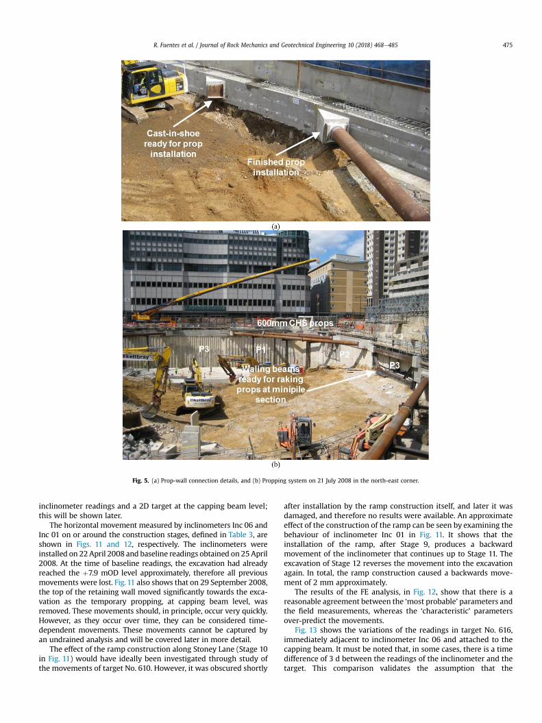
Fig. 5. (a) Prop-wall connection details, and (b) Propping system on 21 July 2008 in the north-east corner.


inclinometer readings and a 2D target at the capping beam level;this will be shown later.

The horizontal movement measured by inclinometers Inc 06 andInc 01 on or around the construction stages, defined in Table 3, areshown in Figs. 11 and 12, respectively. The inclinometers wereinstalled on 22April 2008 and baseline readings obtained on 25April2008. At the time of baseline readings, the excavation had alreadyreached the þ7.9 mOD level approximately, therefore all previousmovements were lost. Fig. 11 also shows that on 29 September 2008,the top of the retaining wall moved significantly towards the exca-vation as the temporary propping, at capping beam level, wasremoved. These movements should, in principle, occur very quickly.However, as they occur over time, they can be considered time-dependent movements. These movements cannot be captured byan undrained analysis and will be covered later in more detail.

The effect of the ramp construction along Stoney Lane (Stage 10in Fig. 11) would have ideally been investigated through study ofthe movements of target No. 610. However, it was obscured shortly

after installation by the ramp construction itself, and later it wasdamaged, and therefore no results were available. An approximateeffect of the construction of the ramp can be seen by examining thebehaviour of inclinometer Inc 01 in Fig. 11. It shows that theinstallation of the ramp, after Stage 9, produces a backwardmovement of the inclinometer that continues up to Stage 11. Theexcavation of Stage 12 reverses the movement into the excavationagain. In total, the ramp construction caused a backwards move-ment of 2 mm approximately.

The results of the FE analysis, in Fig. 12, show that there is areasonable agreement between the ‘most probable’ parameters andthe field measurements, whereas the ‘characteristic’ parametersover-predict the movements.

Fig. 13 shows the variations of the readings in target No. 616,immediately adjacent to inclinometer Inc 06 and attached to thecapping beam. It must be noted that, in some cases, there is a timedifference of 3 d between the readings of the inclinometer and thetarget. This comparison validates the assumption that the

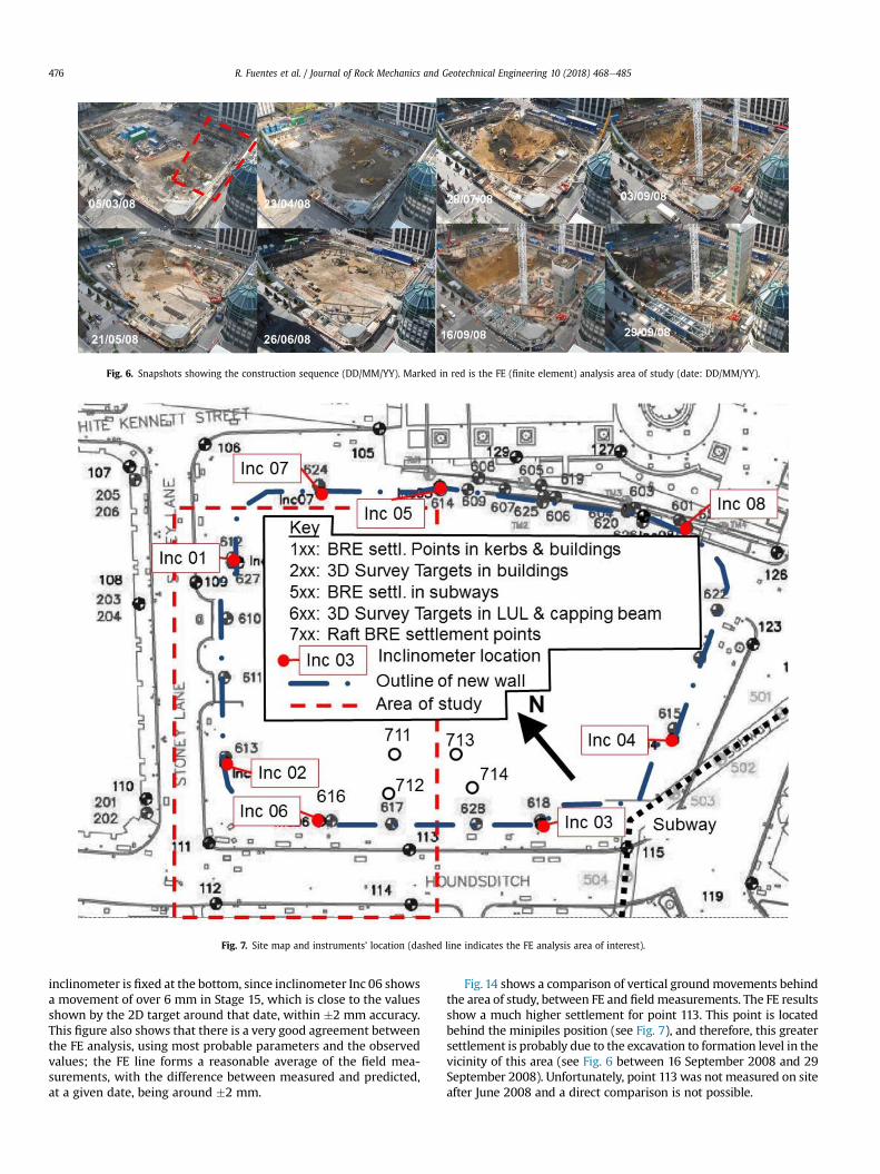
Fig. 6. Snapshots showing the construction sequence (DD/MM/YY). Marked in red is the FE (finite element) analysis area of study (date: DD/MM/YY).

Fig. 7. Site map and instruments’ location (dashed line indicates the FE analysis area of interest).


inclinometer is fixed at the bottom, since inclinometer Inc 06 showsa movement of over 6 mm in Stage 15, which is close to the valuesshown by the 2D target around that date, within �2 mm accuracy.This figure also shows that there is a very good agreement betweenthe FE analysis, using most probable parameters and the observedvalues; the FE line forms a reasonable average of the field mea-surements, with the difference between measured and predicted,at a given date, being around �2 mm.

Fig. 14 shows a comparison of vertical groundmovements behindthe area of study, between FE and field measurements. The FE resultsshow a much higher settlement for point 113. This point is locatedbehind the minipiles position (see Fig. 7), and therefore, this greatersettlement is probably due to the excavation to formation level in thevicinity of this area (see Fig. 6 between 16 September 2008 and 29September 2008). Unfortunately, point 113 was not measured on siteafter June 2008 and a direct comparison is not possible.

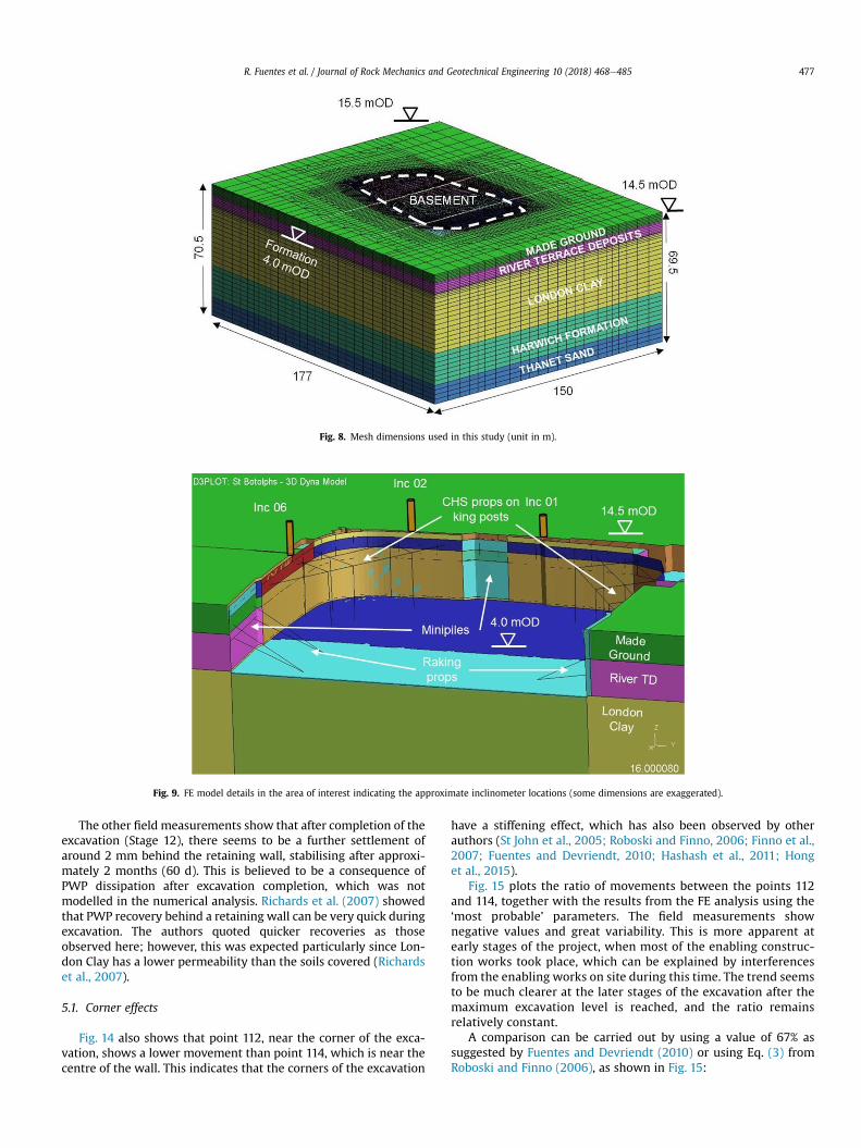
Fig. 8. Mesh dimensions used in this study (unit in m).

Fig. 9. FE model details in the area of interest indicating the approximate inclinometer locations (some dimensions are exaggerated).


The other field measurements show that after completion of theexcavation (Stage 12), there seems to be a further settlement ofaround 2 mm behind the retaining wall, stabilising after approxi-mately 2 months (60 d). This is believed to be a consequence ofPWP dissipation after excavation completion, which was notmodelled in the numerical analysis. Richards et al. (2007) showedthat PWP recovery behind a retaining wall can be very quick duringexcavation. The authors quoted quicker recoveries as thoseobserved here; however, this was expected particularly since Lon-don Clay has a lower permeability than the soils covered (Richardset al., 2007).

5.1. Corner effects

Fig. 14 also shows that point 112, near the corner of the exca-vation, shows a lower movement than point 114, which is near thecentre of the wall. This indicates that the corners of the excavation

have a stiffening effect, which has also been observed by otherauthors (St John et al., 2005; Roboski and Finno, 2006; Finno et al.,2007; Fuentes and Devriendt, 2010; Hashash et al., 2011; Honget al., 2015).

Fig. 15 plots the ratio of movements between the points 112and 114, together with the results from the FE analysis using the‘most probable’ parameters. The field measurements shownegative values and great variability. This is more apparent atearly stages of the project, when most of the enabling construc-tion works took place, which can be explained by interferencesfrom the enabling works on site during this time. The trend seemsto be much clearer at the later stages of the excavation after themaximum excavation level is reached, and the ratio remainsrelatively constant.

A comparison can be carried out by using a value of 67% assuggested by Fuentes and Devriendt (2010) or using Eq. (3) fromRoboski and Finno (2006), as shown in Fig. 15:

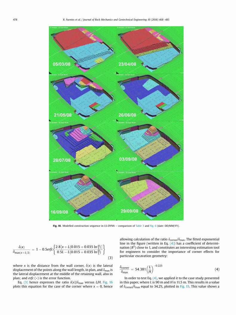
Fig. 10. Modelled construction sequence in LS-DYNA e comparison of Table 3 and Fig. 6 (date: DD/MM/YY).


dðxÞdmaxðx¼ L=2Þ

¼ 1� 0:5erfc

(2:8

�xþ L

�0:015þ 0:035 ln H

L

��0:5L� L

�0:015þ 0:035 ln H

L

�)

(3)

where x is the distance from the wall corner, dðxÞ is the lateraldisplacement of the points along thewall length, in plan, and dmax isthe lateral displacement at the middle of the retaining wall, also inplan; and erfc (,) is the error function.

Eq. (3) hence expresses the ratio d(x)/dmax versus L/H. Fig. 16plots this equation for the case of the corner where x ¼ 0, hence

allowing calculation of the ratio dcorner/dmax. The fitted exponentialline in the figure (written in Eq. (4)) has a coefficient of determi-nation (R2) close to 1, and constitutes an interesting estimation toolfor engineers to consider the importance of corner effects forparticular excavation geometry:

dcornerdmax

¼ 54:381�LH

��0:225(4)

In order to test Eq. (4), we applied it to the case study presentedin this paper, where L is 90 m and H is 11.5 m. This results in a valueof dcorner/dmax equal to 34.2%, plotted in Fig. 15. This value shows a

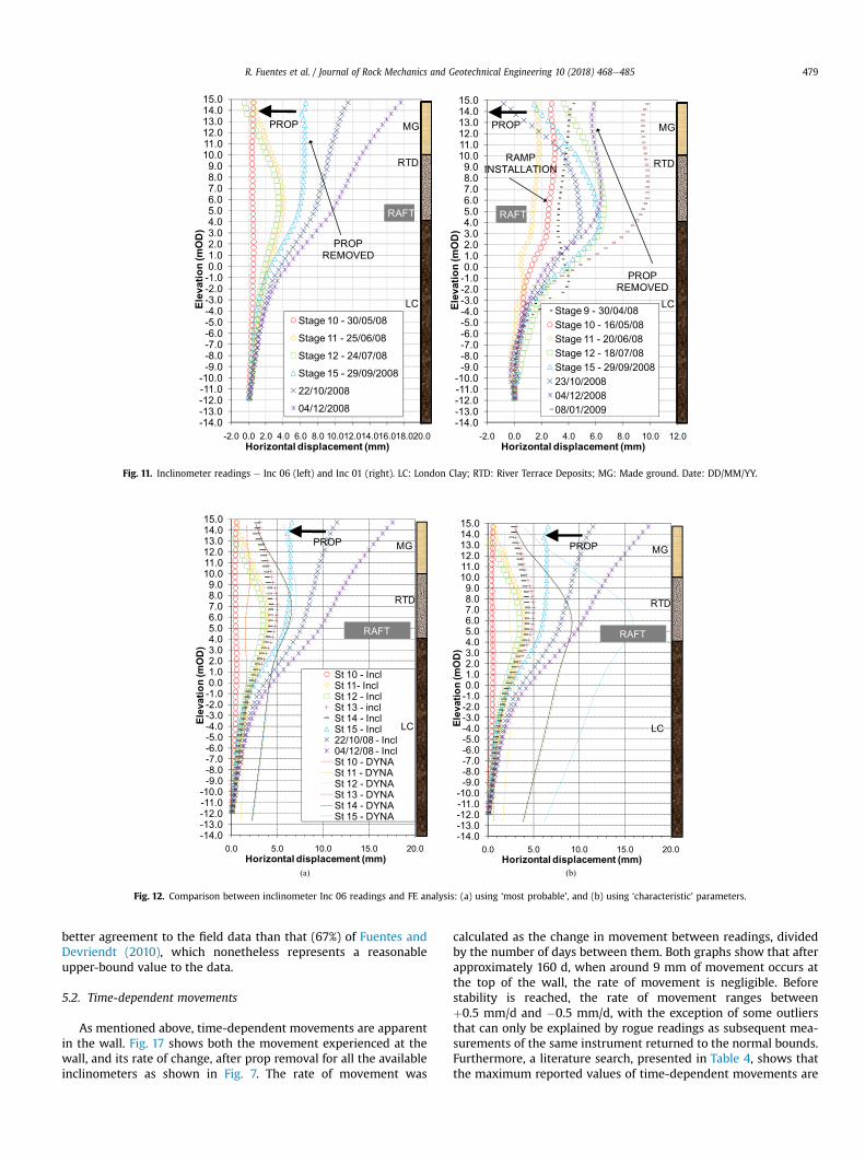
Fig. 11. Inclinometer readings e Inc 06 (left) and Inc 01 (right). LC: London Clay; RTD: River Terrace Deposits; MG: Made ground. Date: DD/MM/YY.

Fig. 12. Comparison between inclinometer Inc 06 readings and FE analysis: (a) using ‘most probable’, and (b) using ‘characteristic’ parameters.


better agreement to the field data than that (67%) of Fuentes andDevriendt (2010), which nonetheless represents a reasonableupper-bound value to the data.

5.2. Time-dependent movements

As mentioned above, time-dependent movements are apparentin the wall. Fig. 17 shows both the movement experienced at thewall, and its rate of change, after prop removal for all the availableinclinometers as shown in Fig. 7. The rate of movement was

calculated as the change in movement between readings, dividedby the number of days between them. Both graphs show that afterapproximately 160 d, when around 9 mm of movement occurs atthe top of the wall, the rate of movement is negligible. Beforestability is reached, the rate of movement ranges betweenþ0.5 mm/d and �0.5 mm/d, with the exception of some outliersthat can only be explained by rogue readings as subsequent mea-surements of the same instrument returned to the normal bounds.Furthermore, a literature search, presented in Table 4, shows thatthe maximum reported values of time-dependent movements are

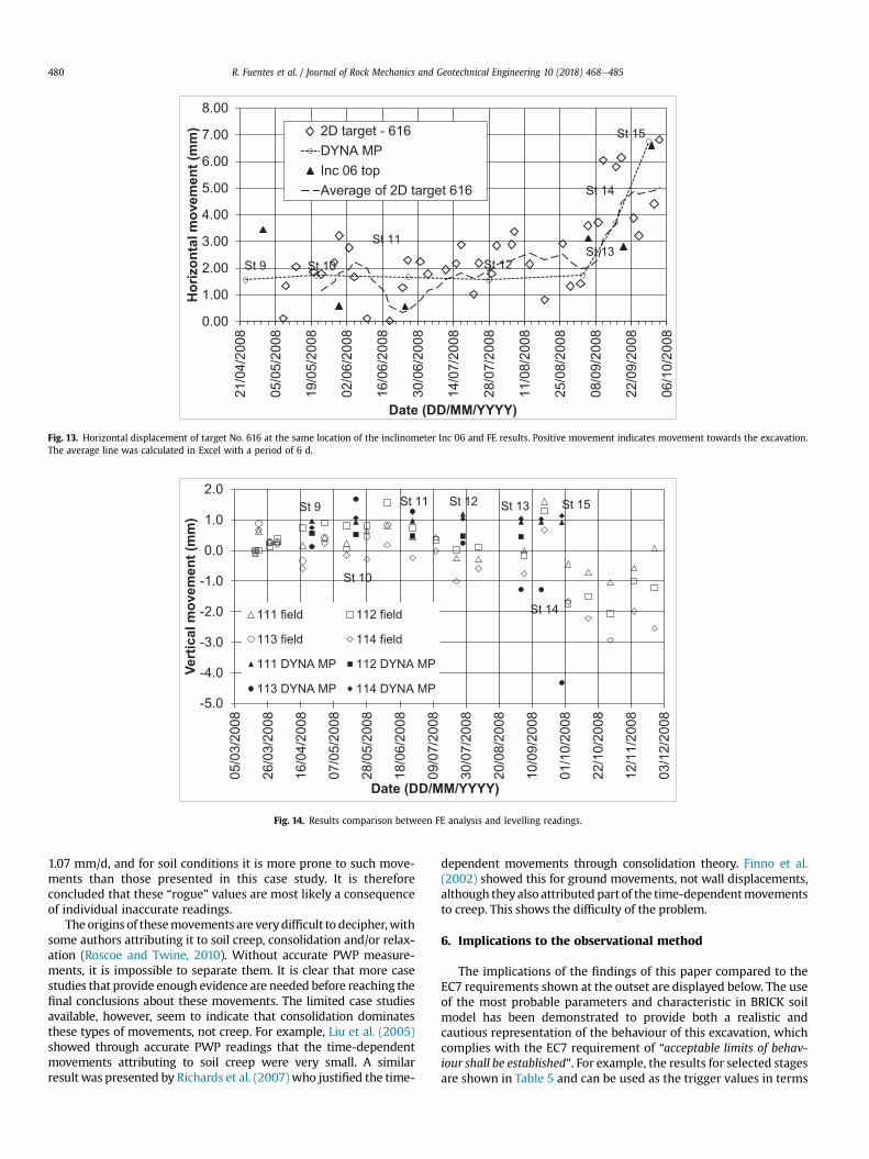
Fig. 13. Horizontal displacement of target No. 616 at the same location of the inclinometer Inc 06 and FE results. Positive movement indicates movement towards the excavation.The average line was calculated in Excel with a period of 6 d.

Fig. 14. Results comparison between FE analysis and levelling readings.


1.07 mm/d, and for soil conditions it is more prone to such move-ments than those presented in this case study. It is thereforeconcluded that these “rogue” values are most likely a consequenceof individual inaccurate readings.

The origins of thesemovements are verydifficult to decipher,withsome authors attributing it to soil creep, consolidation and/or relax-ation (Roscoe and Twine, 2010). Without accurate PWP measure-ments, it is impossible to separate them. It is clear that more casestudies that provide enough evidence are needed before reaching thefinal conclusions about these movements. The limited case studiesavailable, however, seem to indicate that consolidation dominatesthese types of movements, not creep. For example, Liu et al. (2005)showed through accurate PWP readings that the time-dependentmovements attributing to soil creep were very small. A similarresult was presented by Richards et al. (2007)who justified the time-

dependent movements through consolidation theory. Finno et al.(2002) showed this for ground movements, not wall displacements,although theyalso attributed part of the time-dependentmovementsto creep. This shows the difficulty of the problem.

6. Implications to the observational method

The implications of the findings of this paper compared to theEC7 requirements shown at the outset are displayed below. The useof the most probable parameters and characteristic in BRICK soilmodel has been demonstrated to provide both a realistic andcautious representation of the behaviour of this excavation, whichcomplies with the EC7 requirement of “acceptable limits of behav-iour shall be established”. For example, the results for selected stagesare shown in Table 5 and can be used as the trigger values in terms

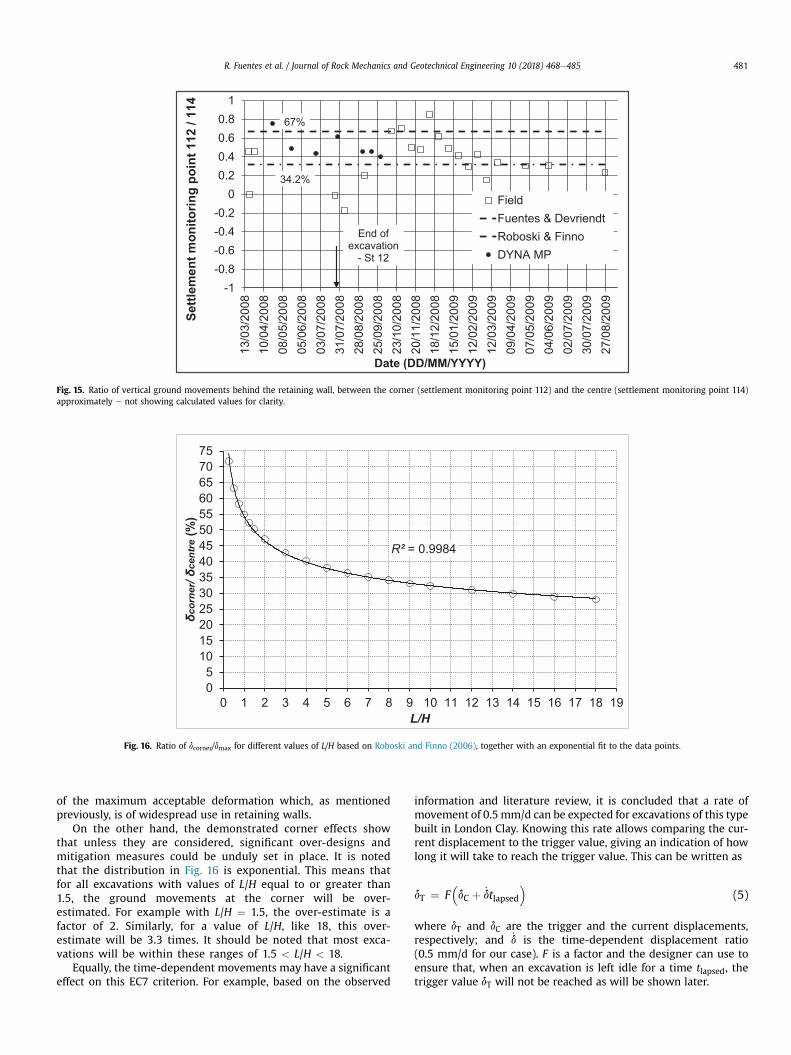
Fig. 15. Ratio of vertical ground movements behind the retaining wall, between the corner (settlement monitoring point 112) and the centre (settlement monitoring point 114)approximately e not showing calculated values for clarity.

Fig. 16. Ratio of dcorner/dmax for different values of L/H based on Roboski and Finno (2006), together with an exponential fit to the data points.


of the maximum acceptable deformation which, as mentionedpreviously, is of widespread use in retaining walls.

On the other hand, the demonstrated corner effects showthat unless they are considered, significant over-designs andmitigation measures could be unduly set in place. It is notedthat the distribution in Fig. 16 is exponential. This means thatfor all excavations with values of L/H equal to or greater than1.5, the ground movements at the corner will be over-estimated. For example with L/H ¼ 1.5, the over-estimate is afactor of 2. Similarly, for a value of L/H, like 18, this over-estimate will be 3.3 times. It should be noted that most exca-vations will be within these ranges of 1.5 < L/H < 18.

Equally, the time-dependent movements may have a significanteffect on this EC7 criterion. For example, based on the observed

information and literature review, it is concluded that a rate ofmovement of 0.5 mm/d can be expected for excavations of this typebuilt in London Clay. Knowing this rate allows comparing the cur-rent displacement to the trigger value, giving an indication of howlong it will take to reach the trigger value. This can be written as

dT ¼ FdC þ _dtlapsed

(5)

where dT and dC are the trigger and the current displacements,respectively; and _d is the time-dependent displacement ratio(0.5 mm/d for our case). F is a factor and the designer can use toensure that, when an excavation is left idle for a time tlapsed, thetrigger value dT will not be reached as will be shown later.

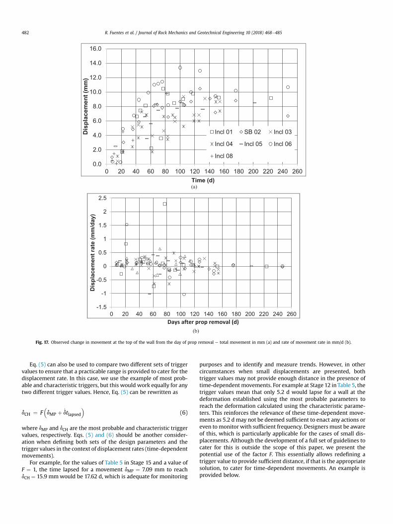
Fig. 17. Observed change in movement at the top of the wall from the day of prop removal e total movement in mm (a) and rate of movement rate in mm/d (b).


Eq. (5) can also be used to compare two different sets of triggervalues to ensure that a practicable range is provided to cater for thedisplacement rate. In this case, we use the example of most prob-able and characteristic triggers, but this would work equally for anytwo different trigger values. Hence, Eq. (5) can be rewritten as

dCH ¼ FdMP þ _dtlapsed

(6)

where dMP and dCH are the most probable and characteristic triggervalues, respectively. Eqs. (5) and (6) should be another consider-ation when defining both sets of the design parameters and thetrigger values in the context of displacement rates (time-dependentmovements).

For example, for the values of Table 5 in Stage 15 and a value ofF ¼ 1, the time lapsed for a movement dMP ¼ 7.09 mm to reachdCH ¼ 15.9 mmwould be 17.62 d, which is adequate for monitoring

purposes and to identify and measure trends. However, in othercircumstances when small displacements are presented, bothtrigger values may not provide enough distance in the presence oftime-dependentmovements. For example at Stage 12 in Table 5, thetrigger values mean that only 5.2 d would lapse for a wall at thedeformation established using the most probable parameters toreach the deformation calculated using the characteristic parame-ters. This reinforces the relevance of these time-dependent move-ments as 5.2 d may not be deemed sufficient to enact any actions oreven tomonitor with sufficient frequency. Designers must be awareof this, which is particularly applicable for the cases of small dis-placements. Although the development of a full set of guidelines tocater for this is outside the scope of this paper, we present thepotential use of the factor F. This essentially allows redefining atrigger value to provide sufficient distance, if that is the appropriatesolution, to cater for time-dependent movements. An example isprovided below.

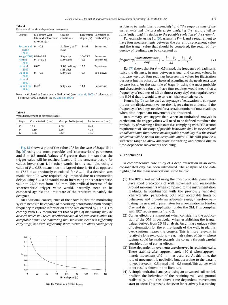
Table 4Database of the time-dependent movements.

Sources Maximum walllateral displacementrate (mm/d)

Groundconditions

Excavationdepth (m)

Constructionmethodology

Roscoe andTwine(2010)1

0.1e0.2 Stiff/very stiffclays

8e16 Bottom-up

Kung (2009) 0.97e1.07 Silty clay 10e23.2 Bottom-upHsiung

(2009)0.14e0.38 Silty sand 19.6 Bottom-up

Liu et al.(2005)

0.051 Soft/medium/stiff clays

15.5 Top-down

Ou et al.(2000)

Lin et al.(2002)

0.1e0.6 Silty clay 19.7 Top-down

Ou and Lai(1994)

0.432 Silty clay 14.4 Bottom-up

Note: 1 calculated as 3 mm over a 60 d period (see Liu et al., 2005). 2 calculated as13 mm over a 60 d period (see Ou and Lai, 1994).

Table 5Wall displacement at different stages.

Stage Characteristic (mm) Most probable (mm) Inclinometer (mm)

15 15.9 7.09 6.4714 9.19 6.56 4.3512 9.06 6.42 3.45


Fig. 18 shows a plot of the value of F for the case of Stage 15 inEq. (6) using the ‘most probable’ and ‘characteristic’ parametersand _d ¼ 0.5 mm/d. Values of F greater than 1 mean that thetrigger value will be reached faster, and the converse occurs forvalues lower than 1. In other words, in this example, using avalue of F ¼ 0.58 means that the lapsed time is 40 d as opposedto 17.62 d as previously calculated for F ¼ 1. If a decision wasmade that 40 d were required, e.g. imposed due to constructiondelays using F ¼ 0.58 would mean increasing the ‘characteristic’value to 27.09 mm from 15.9 mm. This artificial increase of the‘characteristic’ trigger value would, naturally, need to becompared against the limit state of the structure to satisfy thedesigner.

An additional consequence of the above is that the monitoringsystem needs to be capable of measuring deformationwith enoughfrequency to capture information at the rate dictated by _d. This is tocomply with EC7 requirements that “a plan of monitoring shall bedevised, which will reveal whether the actual behaviour lies within theacceptable limits. The monitoring shall make this clear at a sufficientlyearly stage, and with sufficiently short intervals to allow contingency

Fig. 18. Values of F versus tlapsed.

actions to be undertaken successfully” and “the response time of theinstruments and the procedures for analysing the results shall besufficiently rapid in relation to the possible evolution of the system”.

For example, using Eq. (5), assuming F ¼ 1, and a requirement tohave four measurements between the current displacement valueand the trigger value that should be compared, the required fre-quency of readings can be calculated as

frequency�measurements

day

�¼ dT � dC

4 _d¼ dT � dC

2(7)

Eq. (7) shows that for _d ¼ 0.5 mm/d, the frequency of readings istwice the distance, in mm, between trigger and current values. Inthis case, we used four readings between the values for illustrationpurposes but the others can be used according to the needs on a caseby case basis. For the example of Stage 14 using the most probableand characteristic values, to have four readings would mean that afrequency of readings of 1.3 d (almost every day) was required overthe 5.26 d that it would take to reach characteristic value.

Hence, Eq. (7) can be used at any stage of excavation to comparethe current displacement versus the trigger value to understand thefrequency of readings needed for a certain number of total readingswhen time-dependant movements are presented.

In summary, we suggest that, when an undrained analysis iscarried out, the trigger values will need to be defined to reduce theprobability of reaching a limit state (i.e. complying with EC7 secondrequirement of “the range of possible behaviour shall be assessed andit shall be shown that there is an acceptable probability that the actualbehaviour will be within the acceptable limits”). This will provide asufficient range to allow adequate monitoring and actions due totime-dependent movements occurring.

7. Conclusions

A comprehensive case study of a deep excavation in an over-consolidated clay has been introduced. The analysis of the datahighlighted the main observations listed below:

(1) The BRICK soil model using the ‘most probable’ parametersgave good predictions of wall movement and reasonableground movements when compared to the instrumentationreadings. In combination with the previously validated‘characteristic’ parameters, both offer acceptable limits ofbehaviour and provide an adequate range, therefore vali-dating the new set of parameters for an excavation in LondonClay and its future application under the OM. This complieswith EC7 requirements 1 and 2.

(2) Corner effects are important when considering the applica-tion of the OM, in particular when establishing the triggervalues derived from 2D FE analysis. Assuming a unique valueof deformation for the entire length of the wall, in plan, isover-cautious nearer the corners. This is more relevant inrelatively long excavations e e.g. high values of L/H e wheresavings could be made towards the corners through carefulconsideration of corner effects.

(3) Time-dependent movements are observed in retaining walls.These stabilise after approximately 160 d when approxi-mately movement of 9 mm has occurred. At this time, therate of movement is negligible but, according to the data, itranges betweenþ0.5mm/d and�0.5mm/d. This agrees withother results shown in the literature.

(4) A simple undrained analysis, using an advanced soil model,predicts the behaviour of the retaining wall and groundrealistically, until the above time-dependent movementsstart to occur. This means that even for relatively fast moving


construction projects, an undrained analysis using mostprobable parameters may under-predict wall movementsand ground settlement when the site is left idle following theremoval of a prop. This has important implications in theapplication of the OM which relies heavily on accurate apriori definitions of trigger values.

(5) It is therefore recommended that, should an undrainedanalysis be carried out, an additional movement rate shouldbe added to the predicted movements to account for theabove and prevent unwarranted breaches of trigger values.

(6) This case study and others in the literature seem to indicatethat a value of 0.5 mm/d is a reasonable upper-bound valueto use for a wide range of soil types, construction sequencesand excavation depths. However, care must be exercisedwhen defining rates of movement and duration whendefining the trigger values.

(7) Based on all of the above observations in this case study, wehave presented a methodology to consider these time-dependent movements both in the definition of triggervalues and frequency of readings in line with the EC7 re-quirements as shown above.

Conflicts of interest

We wish to confirm that there are no known conflicts of interestassociated with this publication and there has been no significantfinancial support for this work that could have influenced its outcome.

Acknowledgments

The authors would like to acknowledge the EPSRC for theirfunding to undertake this research. Equally we would like to thankMartha Salamanca from Arup for her comments on the manuscriptand help writing it.

References

Atkinson JH, Richardson D, Stallebrass SE. Effect of recent stress history on thestiffness of overconsolidated soil. Géotechnique 1990;40(4):531e40.

British Standards Institute. Geotechnical design Part 1: General rules. Eurocode 7:Geotechnical design - Part 1: General Rules. 2004.

Chapman T, Green G. Observational method looks set to cut city building costs.Proceedings of the Institution of Civil Engineers - Civil Engineering2004;157(3):125e33.

Clarke SD, Hird CC. Modelling of viscous effects in natural clays. CanadianGeotechnical Journal 2012;49(2):129e40.

Ellison KC, Soga K, Simpson B. A strain space soil model with evolving stiffnessanisotropy. Géotechnique 2012;62(7):627e41.

Finno RJ, Bryson S, Calvello M. Performance of a stiff support system in soft clay.Journal of Geotechnical and Geoenvironmental Engineering 2002;128(8):660e71.

Finno RJ, Calvello M. Supported excavations: observational method and inversemodeling. Journal of Geotechnical and Geoenvironmental Engineering2005;131(7):826e36.

Finno RJ, Blackburn JT, Roboski JF. Three-dimensional effects for supported exca-vations in clay. Journal of Geotechnical and Geoenvironmental Engineering2007;133(1):30e6.

FuentesR,DevriendtM.Groundmovements around corners of excavations: empiricalcalculation method. Journal of Geotechnical and Geoenvironmental Engineering2010;136(10). https://doi.org/10.1061/(ASCE)GT.1943-5606.0000347.

Glass PR, Powderham AJ. Application of the observational method at the limehouselink. Géotechnique 1994;44(4):665e79.

Grammatikopoulou A, St John HD, Potts DM. Non-linear and linear models in designof retaining walls. Proceedings of the Institution of Civil Engineers - Geotech-nical Engineering 2008;161(6):311e23.

Hashash YMA, Whittle AJ. Ground movement prediction for deep excavations insoft clay. Journal of Geotechnical Engineering 1996;122(6):474e86.

Hashash YMA, Song H, Osouli A. Three-dimensional inverse analyses of a deepexcavation in Chicago clays. International Journal for Numerical and AnalyticalMethods in Geomechanics 2011;35(9):1059e75.

Hight DW, Gasparre A, Nishimura S, Minh NA, Jardine RJ, Coop MR. Characteristicsof the London clay from the terminal 5 site at heathrow airport. Géotechnique2007;57(1):3e18.

Hong Y, Ng CWW, Liu GB, Liu T. Three-dimensional deformation behaviour of amulti-propped excavation at a ‘greenfield’ site at Shanghai soft clay. Tunnellingand Underground Space Technology 2015;45:249e59.

Hsiung BCB. A case study on the behaviour of a deep excavation in sand. Computersand Geotechnics 2009;36(4):665e75.

Kung GTC. Comparison of excavation-induced wall deflection using top-down andbottom-up construction methods in Taipei silty clay. Computers and Geo-technics 2009;36(3):373e85.

Lin DG, Chung TC, Phien-Wej N. Quantitative evaluation of corner effect on defor-mation behaviour of multi-strutted deep excavation in Bangkok subsoil. Journalof the Southeast Asian Geotechnical Society 2003;34(1):41e57.

Lin HD, Ou CY, Wang CC. Time-dependent displacement of diaphragmwall inducedby soil creep. Journal of the Chinese Institute of Engineers 2002;25(2):223e31.

Liu GB, Ng CWW, Wang ZW. Observed performance of a deep multistrutted exca-vation in Shanghai soft clays. Journal of Geotechnical and GeoenvironmentalEngineering 2005;131(8):1004e13.

Long M. A case history of a deep basement in London Clay. Computers and Geo-technics 2001;28(6e7):397e423.

LS-DYNA. Civil engineering application program. 2008. Oasys Limited, LivermoreSoftware Technology Corporation, Version 940.

Ng CW, Simpson B, Lings ML, Nash D. Numerical analysis of a multipropped exca-vation in stiff clay. Canadian Geotechnical Journal 1998;35(1):115e30.

Nicholson D, Tse CM, Penny C. The observational method in ground engineering:principles and applicationsvol. 185. CIRIA; 1999.

Nicholson D, Yeow HC, Black M, Glass P, Man CL, Ringer A. Application of obser-vational method at crossrail tottenham court road station, UK. Proceedings ofthe Institution of Civil Engineers - Geotechnical Engineering 2014;167(2):182e93.

Ou CY, Lai CH. Finite-element analysis of deep excavation in layered sandy andclayey soil deposits. Canadian Geotechnical Journal 1994;31(2):204e14.

Ou CY, Liao JT, Cheng WL. Building response and ground movements induced by adeep excavation. Géotechnique 2000;50(3):209e20.

Pantelidou H, Impson BS. Geotechnical variation of London clay across centralLondon. Géotechnique 2007;57(1):101e12.

Peck RB. Advantages and limitations of the observational method in applied soilmechanics. Géotechnique 1969;19(2):171e87.

Peck RB. The observational method can be simple. Proceedings of the Institution ofCivil Engineers - Geotechnical Engineering 2001;149(2):71e4.

Pillai A. Review of the BRICK model of soil behaviour. Imperial College London;1996.

Potts DM, Zdravkovic L. Finite element analysis in geotechnical engineering: vol-ume two - Application. Thomas Telford Publishing; 2001.

Powderham AJ. An overview of the observational method: development in cut andcover and bored tunnelling projects. Géotechnique 1994;44(4):619e36.

Powderham AJ, Rutty P. The observational method in value engineering. In: Pro-ceedings of 5 th international conference & exhibition on piling and deepfoundations. Bruges, Belgium: Deep Foundations Institute; 1994.

Powderham AJ. The observational method - learning from projects. Proceedings of theInstitution of Civil Engineers - Geotechnical Engineering 2002;115(1):59e69.

Prästings A, Müller R, Larsson S. The observational method applied to a highembankment founded on sulphide clay. Engineering Geology 2014;181:112e23.

Richards DJ, Powrie W, Roscoe H, Clark J. Pore water pressure and horizontal stresschanges measured during construction of a contiguous bored pile multi-propped retaining wall in Lower Cretaceous clays. Géotechnique 2007;57(2):197e205.

Roboski J, Finno RJ. Distributions of ground movements parallel to deep excavationsin clay. Canadian Geotechnical Journal 2006;43(1):43e58.

Roscoe H, Twine D. Design and performance of retaining walls. Proceedings of theInstitution of Civil Engineers - Geotechnical Engineering 2010;163(5):279e90.

Sakurai S, Akutagawa S, Takeuchi K, Shinji M, Shimizu N. Back analysis for tunnelengineering as a modern observational method. Tunnelling and UndergroundSpace Technology 2003;18(2e3):185e96.

Simpson B. Retaining structures: displacement and design. Géotechnique1992;42(4):541e76.

Spross J, Johansson F. When is the observational method in geotechnical engi-neering favourable? Structural Safety 2017;66:17e26.

Spross J, Johansson F, Uotinen LKT, Rafi JY. Using observational method to managesafety aspects of remedial grouting of concrete dam foundations. Geotechnicaland Geological Engineering 2016;34(5):1613e30.

St John HD, Zdravkovic L, Potts DM. Modelling of a 3D excavation in finite elementanalysis. Géotechnique 2005;55(7):497e513.

Steel Construction Institute. Steelwork design guide to BS 5950-1:2000. Vol. 1,Section properties, member capacities. 2007. Steel Construction Institute.

Whittle AJ, Hashash YMA. Analysis of the behaviour of propped diaphragmwalls ina deep clay deposit. In: Retaining structures, proceedings of the conference.Cambridge, UK: Thomas Telford Publishing; 1992. p. 131e9.

Yeow HC, Nicholson DP, Simpson B. Comparison and feasibility of three dimensionalfinite element modelling of deep excavations using non-linear soil models. In:Numerical modelling of construction processes in geotechnical engineering forurban environment. CRC Press; 2006. p. 29e34.

Yeow H, Feltham I. Case histories back analyses for the application of the obser-vational method under Eurocodes for the Scout project. In: The 6th interna-tional conference on case histories in geotechnical engineering. Arlington, VA,USA: Missouri University of Science and Technology; 2008. p. 1e13.

http://refhub.elsevier.com/S1674-7755(17)30302-5/sref1


























https://doi.org/10.1061/(ASCE)GT.1943-5606.0000347





































































































































Raul Fuentes is an Associate Professor in InfrastructureEngineering at the University of Leeds (UK). Before joiningthe University of Leeds, Raul worked as a Lecturer in UCL,and previously in industry for companies like Atkins, MayGurney and Arup where he gained substantial experiencein the planning, design and delivery of diverse civil engi-neering projects. He is still actively involved with practiceacting as consultant in projects in the areas of instru-mentation and monitoring, tunnelling and ground engi-neering. His research interests can divided into threedistinct topics all contributing to the overarching theme ofResilient Infrastructure: (1) “Disruptive technologies” ininfrastructure - Robotics and Autonomous Systems,Structure-from-motion - SfM, BIM, laser scanning, photo-

grammetry, fibre optics, structural health monitoring and remote sensing. (2) “Flowingground” and its interaction with structures - Landslides, geotechnical earthquake en-gineering, lateral spreading and soil erosion with a view to quantify their impact onthe national infrastructure using complex soil-structure-fluid interaction methods.(3) “Energy geotechnics” - Geothermal and other heat recovery systems, geothermalpiles, walls, tunnels and other structures, thermo-hydro-mechanical modelling of soils.He is a Chartered Engineer and member of the Institution of Civil Engineers (UK).

Anton Pillai is an Associate at Arup, London. He has 23years’ experience in the UK and in South East Asia on awide variety of projects, specialising in the geotechnicaldesign of underground, offshore and maritime structures.He is the team leader for modelling and analyses of com-plex 2D and 3D geotechnical, tunnelling and offshoreproblems. He is also responsible for reviews of results andinterpretations of 2D and 3D finite element (FE) analysesdone by others. His expertise covers advanced soil-structure interaction analysis of masonry and cast irontunnels, deep excavations in complex geology, andoffshore foundations for both gravity and jacket type pro-duction platforms.

Dr. Pedro Ferreira is a senior lecturer at University CollegeLondon (UCL). He graduated from Federal University of RioGrande do Sul/Porto Alegre in 1998, his MSc in Geotech-nical Engineering in 1998 and his PhD, in the same area, in2002. He worked as a Post-doc at Imperial College from2003 to 2005, when he joined UCL as a Lecturer. He isalso the soil mechanics laboratory manager, responsiblefor a large number of geotechnical equipment. To thisdate, he has supervised the following: 5 PhD students;more than 40 MSc students and is currently supervisinga further 5 PhD students. The topics of Pedro’s researchinclude: finite element analysis applied to excavationsand tunnels; new monitoring techniques to aid asset man-agement and monitoring deformations; single element

testing; sprayed concrete technology applied to tunnels and reinforced soils with fibresand cement, with the aim of reducing maintenance of geotechnical structures. Hisresearch interests are connected to geotechnical engineering and he has contactswith many industry partners in UK and many universities in Europe, Asia and SouthAmerica. He is also the author of many research papers in the above mentionedsubjects.

Documents

Lessons learnt from a deep excavation for future …eprints.whiterose.ac.uk/125771/15/Lessons learnt from a...Full Length Article Lessons learnt from a deep excavation for future application