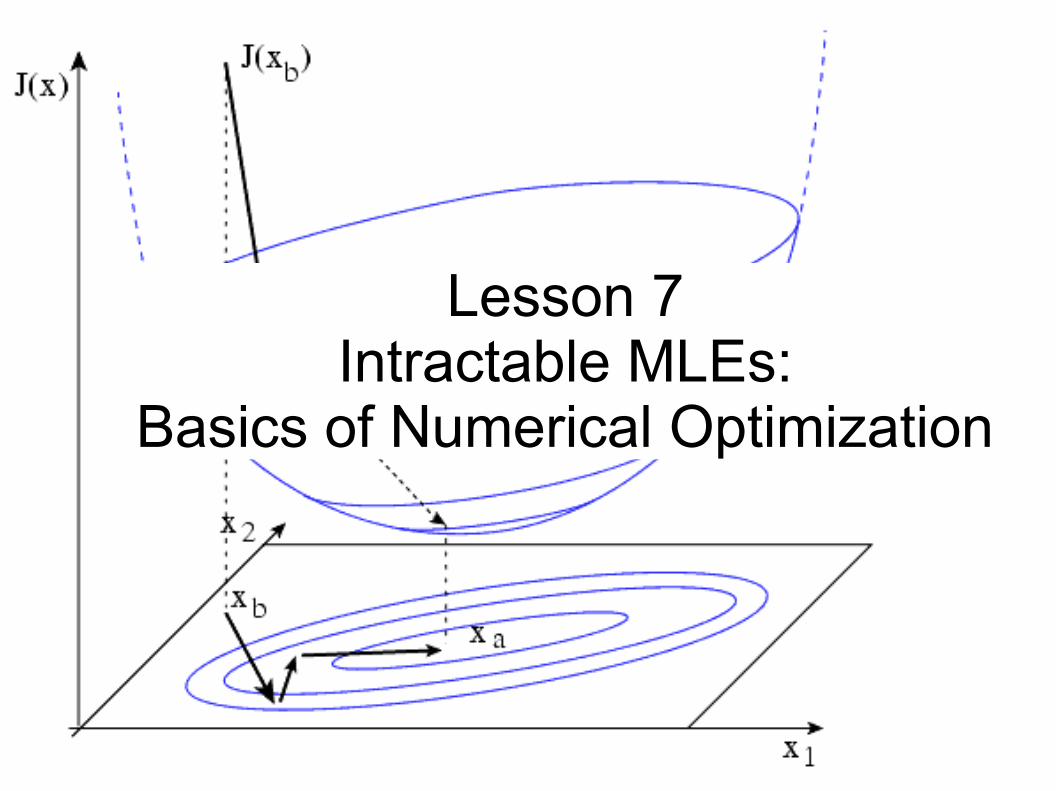
Lesson 7Intractable MLEs:

Basics of Numerical Optimization

Maximum Likelihood

Write down the Likelihood

Take the log

Take the derivatives w.r.t. each parameter

Set equal to 0 and solve for parameterMaximum Likelihood Estimate (MLE)

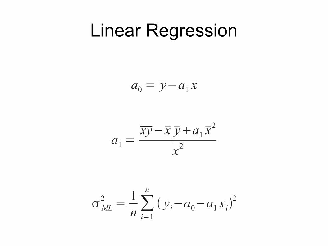
Linear Regression

a0 = y−a1x

a1 =xy−x ya1x

2

x2

ML2 = 1

n∑i=1

n

yi−a0−a1 xi2

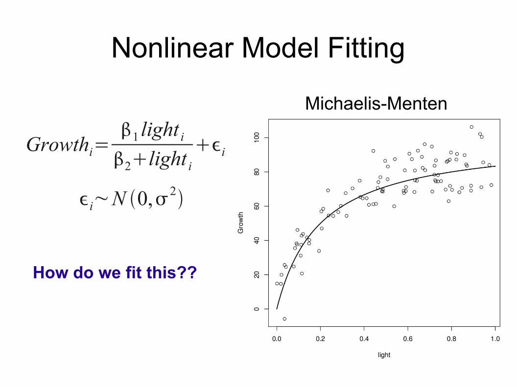
Nonlinear Model Fitting

Growthi=1 light i2light i

i

i~N 0, 2

Michaelis-Menten

How do we fit this??

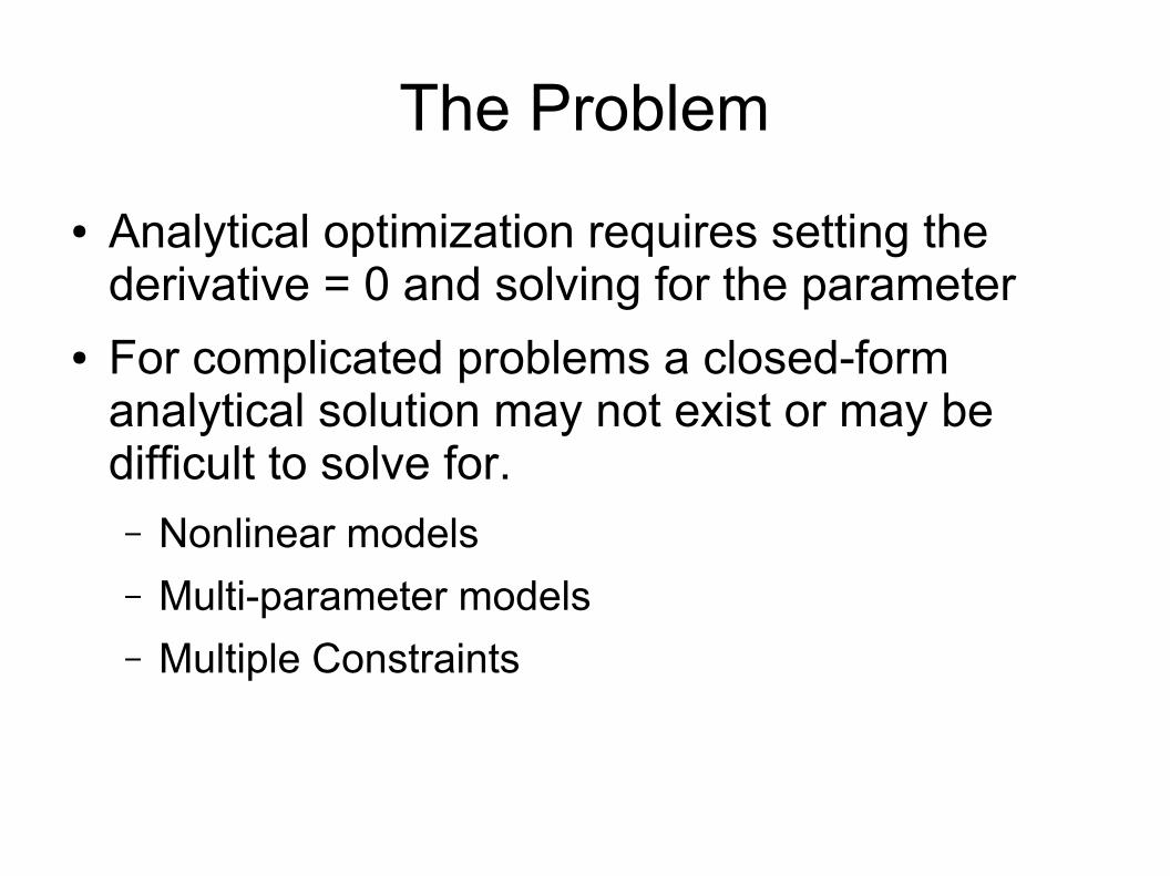
The Problem

● Analytical optimization requires setting thederivative = 0 and solving for the parameter

● For complicated problems a closed-formanalytical solution may not exist or may bedifficult to solve for.– Nonlinear models

– Multi-parameter models

– Multiple Constraints

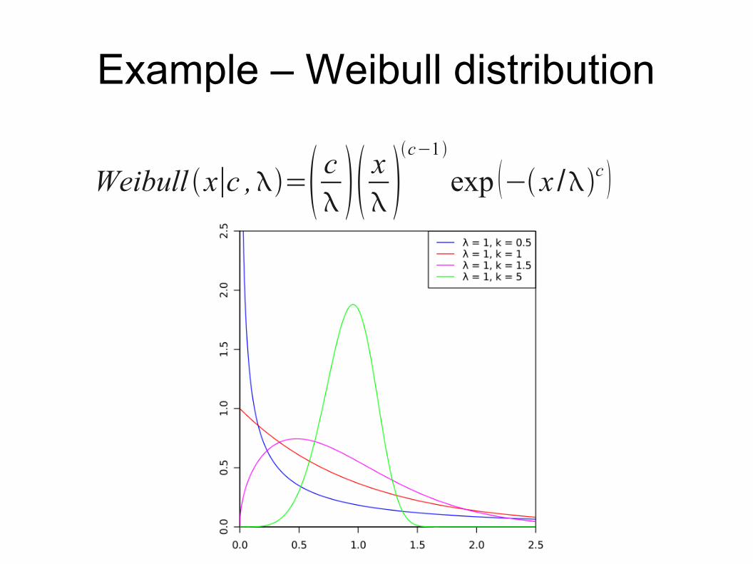
Example – Weibull distribution

Weibull x∣c ,= c x c−1

exp − x /c

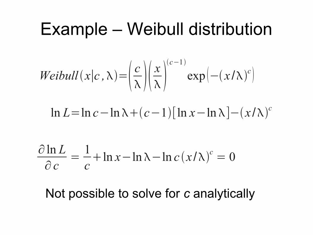
Example – Weibull distribution

Weibull x∣c ,= c x c−1

exp − x /c

ln L=ln c−lnc−1[ ln x−ln]−x /c

∂ ln L∂ c

= 1cln x−ln−ln c x /c = 0

Not possible to solve for c analytically

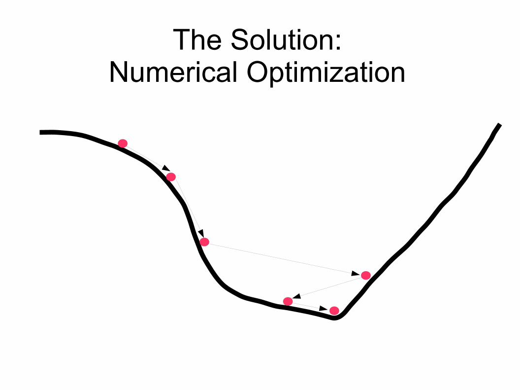
The Solution:Numerical Optimization

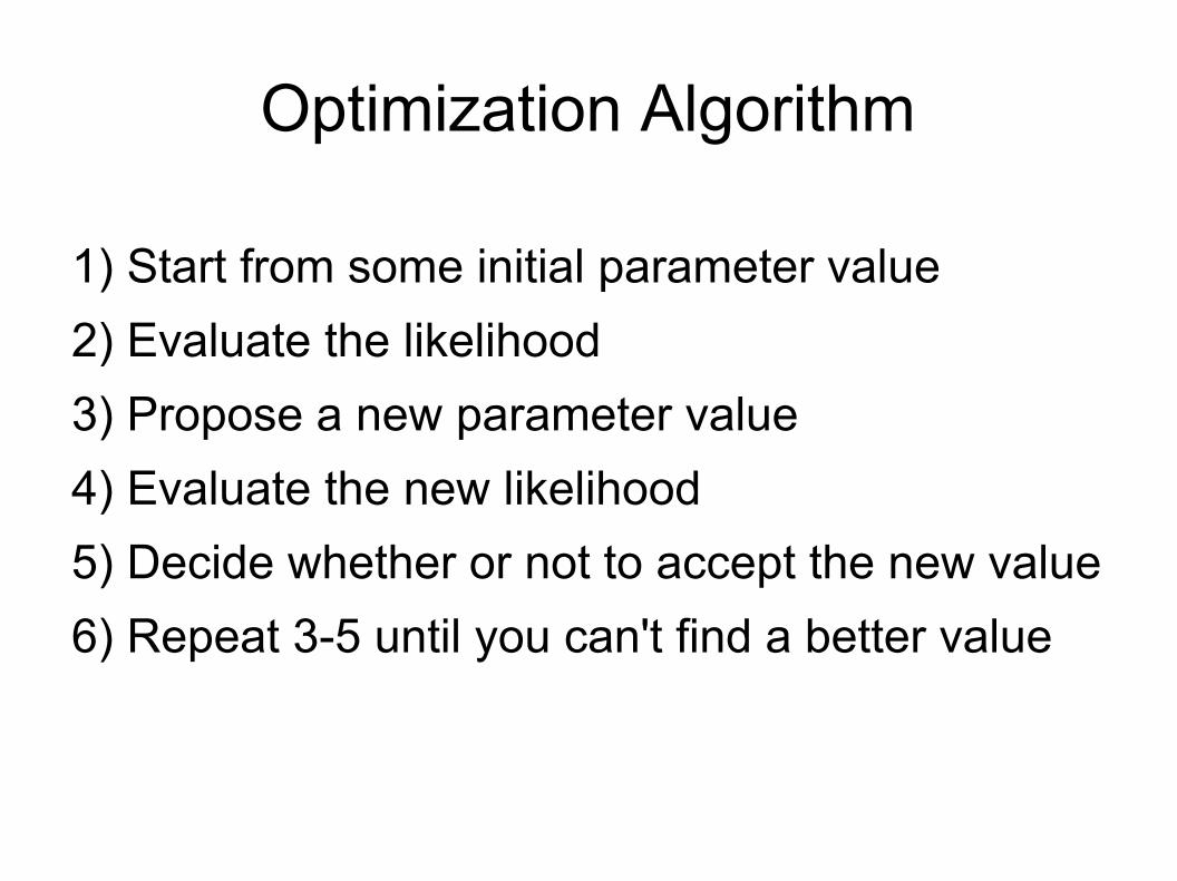
Optimization Algorithm

1) Start from some initial parameter value

2) Evaluate the likelihood

3) Propose a new parameter value

4) Evaluate the new likelihood

5) Decide whether or not to accept the new value

6) Repeat 3-5 until you can't find a better value

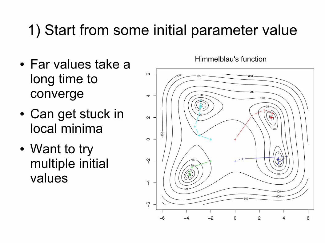
1) Start from some initial parameter value

● Far values take along time toconverge

● Can get stuck inlocal minima

● Want to trymultiple initialvalues

Himmelblau's function

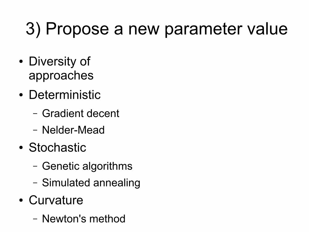
3) Propose a new parameter value

● Diversity ofapproaches

● Deterministic– Gradient decent

– Nelder-Mead

● Stochastic– Genetic algorithms

– Simulated annealing

● Curvature– Newton's method

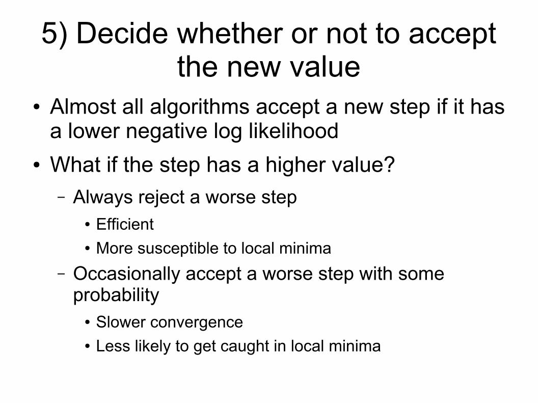
5) Decide whether or not to acceptthe new value

● Almost all algorithms accept a new step if it hasa lower negative log likelihood

● What if the step has a higher value?– Always reject a worse step

● Efficient● More susceptible to local minima

– Occasionally accept a worse step with someprobability

● Slower convergence● Less likely to get caught in local minima

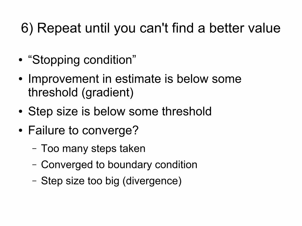
6) Repeat until you can't find a better value

● “Stopping condition”● Improvement in estimate is below some

threshold (gradient)● Step size is below some threshold● Failure to converge?

– Too many steps taken

– Converged to boundary condition

– Step size too big (divergence)

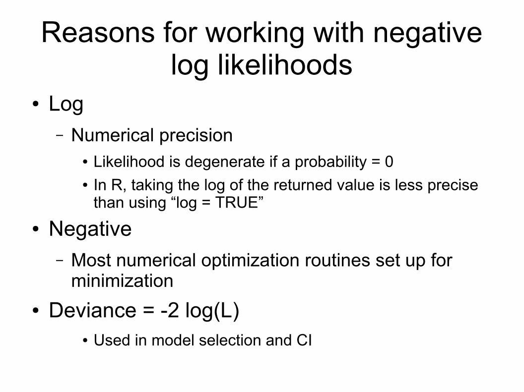
Reasons for working with negativelog likelihoods

● Log – Numerical precision

● Likelihood is degenerate if a probability = 0● In R, taking the log of the returned value is less precise

than using “log = TRUE”

● Negative– Most numerical optimization routines set up for

minimization

● Deviance = -2 log(L)● Used in model selection and CI

Optimization Algorithm

1) Start from some initial parameter value

2) Evaluate the likelihood

3) Propose a new parameter value

4) Evaluate the new likelihood

5) Decide whether or not to accept the new value

6) Repeat 3-5 until you can't find a better value

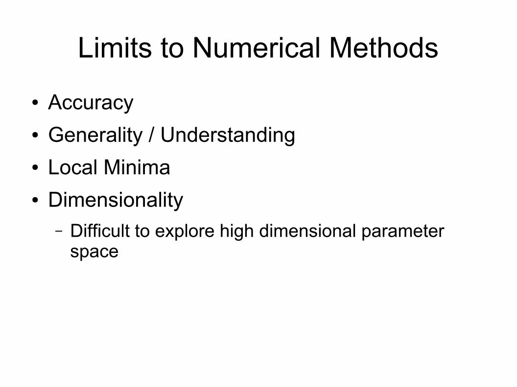
Limits to Numerical Methods

● Accuracy● Generality / Understanding● Local Minima● Dimensionality

– Difficult to explore high dimensional parameterspace

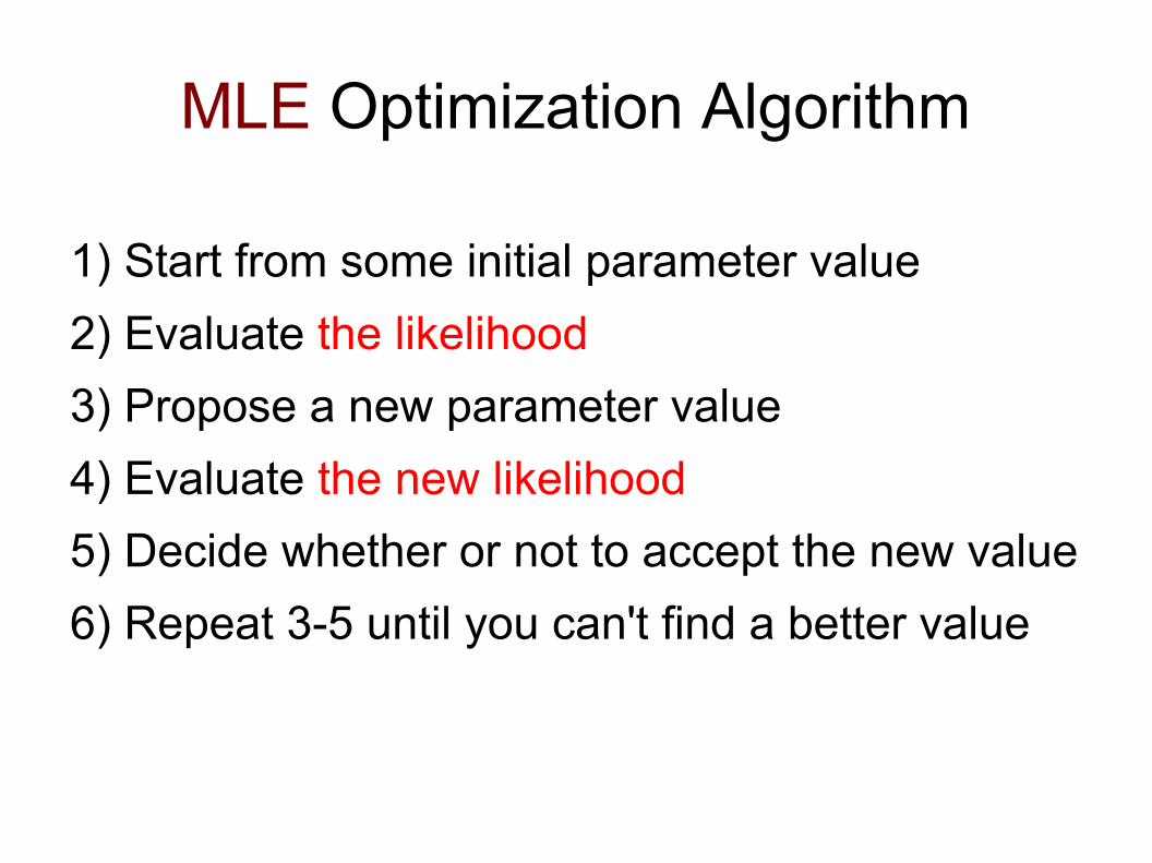
MLE Optimization Algorithm

1) Start from some initial parameter value

2) Evaluate the likelihood

3) Propose a new parameter value

4) Evaluate the new likelihood

5) Decide whether or not to accept the new value

6) Repeat 3-5 until you can't find a better value

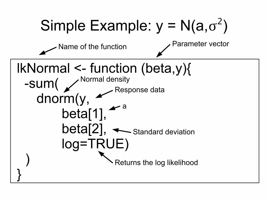
lkNormal <- function (beta,y){ -sum(

dnorm(y,beta[1],

beta[2],log=TRUE)

) }

Response data

Returns the log likelihood

Standard deviation

a

Name of the function Parameter vector

Normal density

Simple Example: y = N(a,s2)

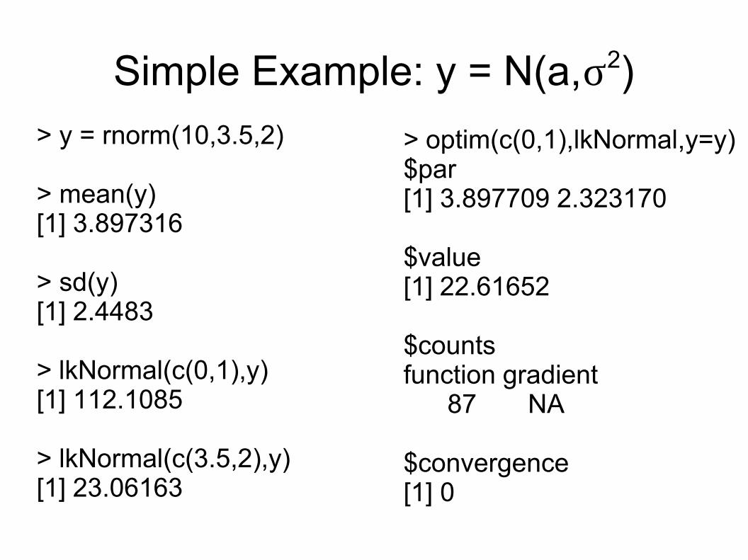
Simple Example: y = N(a,s2)

> y = rnorm(10,3.5,2)

> mean(y)[1] 3.897316

> sd(y)[1] 2.4483

> lkNormal(c(0,1),y)[1] 112.1085

> lkNormal(c(3.5,2),y)[1] 23.06163

> optim(c(0,1),lkNormal,y=y)$par[1] 3.897709 2.323170

$value[1] 22.61652

$countsfunction gradient 87 NA

$convergence[1] 0

Nonlinear example

Growthi=1 light i2light i

i

i~N 0, 2

“Pseudodata”b

1 = 100

b2 = 0.2

s = 10n = 100

Michaelis-Menten

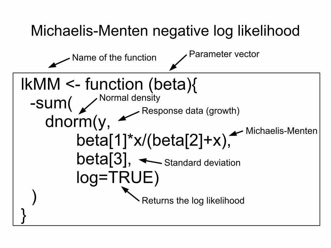
lkMM <- function (beta){ -sum(

dnorm(y,beta[1]*x/(beta[2]+x),

beta[3],log=TRUE)

) }

Response data (growth)

Returns the log likelihood

Standard deviation

Michaelis-Menten

Name of the function Parameter vector

Normal density

Michaelis-Menten negative log likelihood

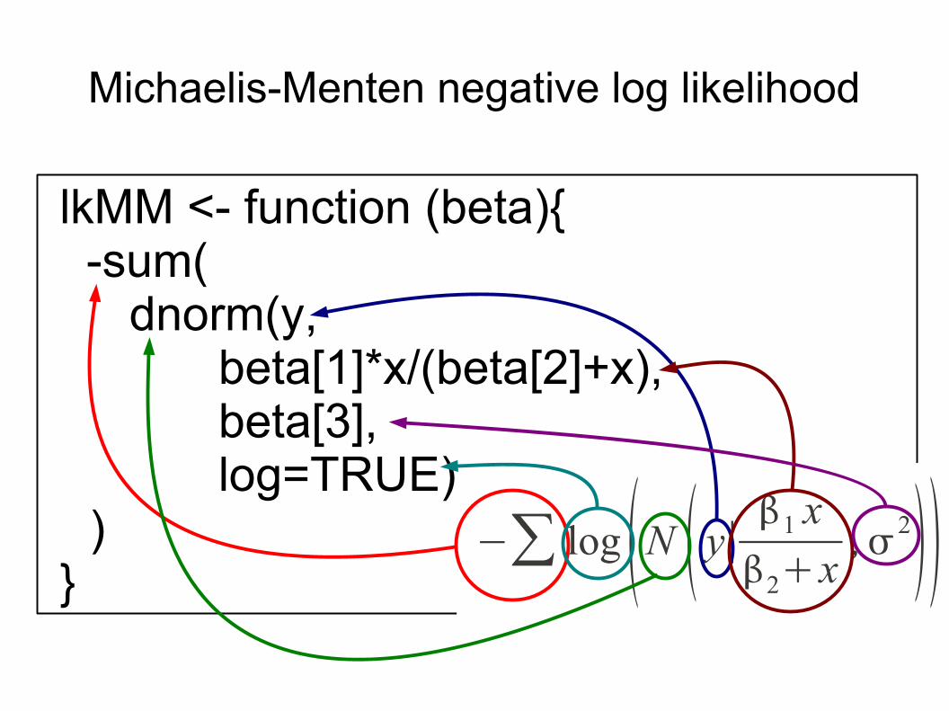
lkMM <- function (beta){ -sum(

dnorm(y,beta[1]*x/(beta[2]+x),

beta[3],log=TRUE)

) }

Michaelis-Menten negative log likelihood

−∑ log N y∣ 1 x

2x, 2

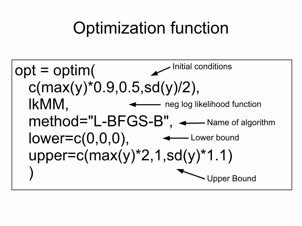
opt = optim(c(max(y)*0.9,0.5,sd(y)/2),lkMM,method="L-BFGS-B",lower=c(0,0,0),upper=c(max(y)*2,1,sd(y)*1.1))

Optimization function

Initial conditions

neg log likelihood function

Name of algorithm

Lower bound

Upper Bound

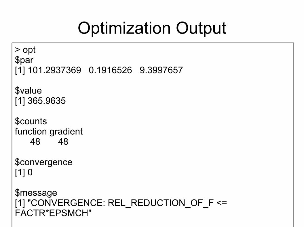
> opt$par[1] 101.2937369 0.1916526 9.3997657

$value[1] 365.9635

$countsfunction gradient 48 48

$convergence[1] 0

$message[1] "CONVERGENCE: REL_REDUCTION_OF_F <=FACTR*EPSMCH"

Optimization Output

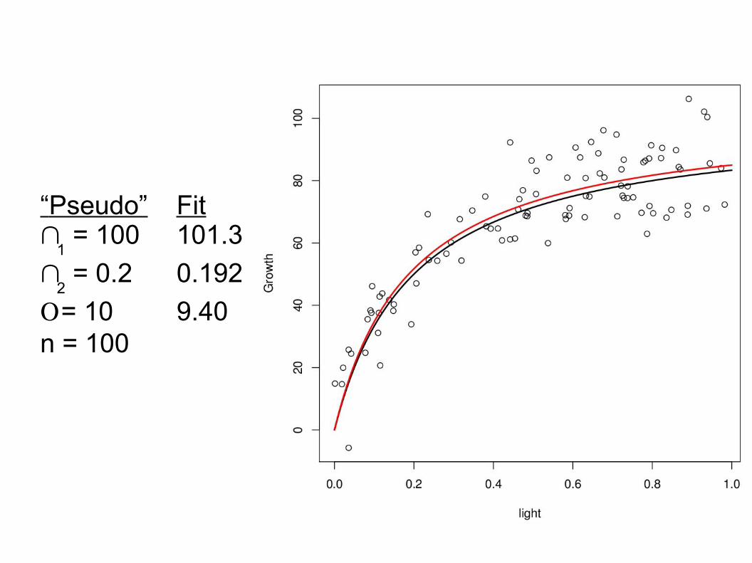
“Pseudo” Fitb

1 = 100 101.3

b2 = 0.2 0.192

s = 10 9.40n = 100

More generally...

● Can fit any 'black box' function● Can use any distribution

– No Normality assumption

● Can model the variance explicitly– No equal variance assumption

● Various techniques for estimating uncertainties,CI, etc.

● Likelihood is backbone of more advancedapproaches (e.g. Bayesian stats)

A few last thoughts on MLE

● More difficult as model complexity increases● More challenging when not independent

P(x1,x2,x3) ≠ P(x1)P(x2)P(x3)● Require additional assumptions/computation to

estimate CI● Analysis occurs in a “vacuum”

– No way to update previous analysis