Lesson 5 – Introduction to Exponential Functions · PDF file · 2014-06-122014-06-12 · Lesson 5 – Introduction to Exponential Functions ... $1000 to start + $1000 per day Option

Page 169

Lesson 5 – Introduction to Exponential Functions Exponential Functions play a major role in our lives. Many of the challenges we face involve exponential change and can be modeled by an Exponential Function. Financial considerations are the most obvious, such as the growth of our retirement savings, how much interest we are paying on our home loan or the effects of inflation. In this lesson, we begin our investigation of Exponential Functions by comparing them to Linear Functions, examining how they are constructed and how they behave. We then learn methods for solving exponential functions given the input and given the output. Lesson Topics:

Section 5.1: Linear Functions Vs. Exponential Functions

§ Characteristics of linear functions § Comparing linear and exponential growth § Using the common ratio to identify exponential data § Horizontal Intercepts

Section 5.2: Characteristics of Exponential Functions Section 5.3: Solving Exponential Equations by Graphing

§ Using the Intersect Method to solve exponential equations on the graphing calculator

§ Guidelines for setting an appropriate viewing window

Section 5.4: Applications of Exponential Functions

Page 170

Lesson 5 Checklist

Component Required? Y or N Comments Due Score

Mini-Lesson

Online Homework

Online Quiz

Online Test

Practice Problems

Lesson Assessment

Name: _____________________________ Date: ________________

Page 171

Mini-Lesson 5

Section 5.1 – Linear Functions vs. Exponential Functions

Problem 1 YOU TRY – Characteristics of Linear Functions Given a function, f(x) = mx + b, respond to each of the following. Refer back to previous lessons as needed.

a) The variable x represents the __________________ quantity.

b) f(x) represents the _________________ quantity.

c) The graph of f is a _________________________________ with slope __________ and

vertical intercept _________________ .

d) On the graphing grid below, draw an INCREASING linear function. In this case, what

can you say about the slope of the line? m ______ 0 (Your choices here are > or <)

e) On the graphing grid below, draw a DECREASING linear function. In this case, what

can you say about the slope of the line? m ______ 0 (Your choices here are > or <)

f) The defining characteristic of a LINEAR FUNCTION is that the RATE OF CHANGE

(also called the SLOPE) is _______________________.

g) The domain of a LINEAR FUNCTION is _____________________________________

Lesson 5 – Introduction to Exponential Functions Mini-Lesson

Page 172

This next example is long but will illustrate the key difference between EXPONENTIAL FUNCTIONS and LINEAR FUNCTIONS. Problem 2 WORKED EXAMPLE – DOLLARS & SENSE On December 31st around 10 pm, you are sitting quietly in your house watching Dick Clark's New Year's Eve special when there is a knock at the door. Wondering who could possibly be visiting at this hour you head to the front door to find out who it is. Seeing a man dressed in a three-piece suit and tie and holding a briefcase, you cautiously open the door. The man introduces himself as a lawyer representing the estate of your recently deceased great uncle. Turns out your uncle left you some money in his will, but you have to make a decision. The man in the suit explains that you have three options for how to receive your allotment. Option A: $1000 would be deposited on Dec 31st in a bank account bearing your name and each

day an additional $1000 would be deposited (until January 31st). Option B: One penny would be deposited on Dec 31st in a bank account bearing your name.

Each day, the amount would be doubled (until January 31st). Option C: Take $30,000 on the spot and be done with it. Given that you had been to a party earlier that night and your head was a little fuzzy, you wanted some time to think about it. The man agreed to give you until 11:50 pm. Which option would give you the most money after the 31 days??? A table of values for option A and B are provided on the following page. Before you look at the values, though, which option would you select according to your intuition?

Without “doing the math” first, I would instinctively choose the following option (circle your choice):

Option Option Option

A B C


Page 173

Option A: $1000 to start + $1000 per day

Option B: $.01 to start then double each day

Note that t = 0 on Dec. 31st Table of input/output values

t = time in # of days since Dec 31

A(t)=$ in account after t days

0 1000 1 2000 2 3000 3 4000 4 5000 5 6000 6 7000 7 8000 8 9000 9 10,000 10 11,000 11 12,000 12 13,000 13 14,000 14 15,000 15 16,000 16 17,000 17 18,000 18 19,000 19 20,000 20 21,000 21 22,000 22 23,000 23 24,000 24 25,000 25 26,000 26 27,000 27 28,000 28 29,000 29 30,000 30 31,000 31 32,000

Table of input/output values t = time

in # of days since Dec 31

B(t) = $ in account after t days

0 .01 1 .02 2 .04 3 .08 4 .16 5 .32 6 .64 7 1.28 8 2.56 9 5.12 10 10.24 11 20.48 12 40.96 13 81.92 14 163.84 15 327.68 16 655.36 17 1,310.72 18 2,621.44 19 5,242.88 20 10,485.76 21 20,971.52 22 41,943.04 23 83,886.08 24 167,772.16 25 335,544.32 26 671,088.64 27 1,342,177.28 28 2,684,354.56 29 5,368,709.12 30 10,737,418.24 31 21,474,836.48

WOWWWWW!!!!!!! What IS that number for Option B? I hope you made that choice… it’s 21 million, 4 hundred 74 thousand, 8 hundred 36 dollars and 48 cents. Let’s see if we can understand what is going on with these different options.


Page 174

Problem 3 MEDIA EXAMPLE – Compare Linear and Exponential Growth For the example discussed in Problem 2, respond to the following: a) Symbolic representation (model) for each situation: A(t) =

Type of function __________________

B(t) =


C(t) =


b) Provide a rough but accurate sketch of the graphs for each function on the same grid below:

c) What are the practical domain and range for each function? Practical Domain Practical Range A(t):

B(t):

C(t):

d) Based on the graphs, which option would give you the most money after 31 days?


Page 175

e) Let’s see if we can understand WHY option B grows so much faster. Let’s focus just on options A and B. Take a look at the data tables given for each function. Just the later parts of the initial table are provided.

A(t) = 1000t + 1000

t = time in # of days since Dec 31

A(t)=$ in account after t

days 20 21,000 21 22,000 22 23,000 23 24,000 24 25,000 25 26,000 26 27,000 27 28,000 28 29,000 29 30,000 30 31,000 31 32,000

B(t) = .01(2)t

t =time in # of days since Dec 31

B(t) = $ in account after t

days 20 10,485.76 21 20,971.52 22 41,943.04 23 83,886.08 24 167,772.16 25 335,544.32 26 671,088.64 27 1,342,177.28 28 2,684,354.56 29 5,368,709.12 30 10,737,418.24 31 21,474,836.48

As t increases from day 20 to 21, describe how the outputs change for each function:

A(t): B(t):

As t increases from day 23 to 24, describe how the outputs change for each function: A(t): B(t):

So, in general, we can say as the inputs increase from one day to the next, then the outputs for each function:

A(t): B(t):

In other words, A(t) grows _____________________ and B(t) grows _____________________.


Page 176

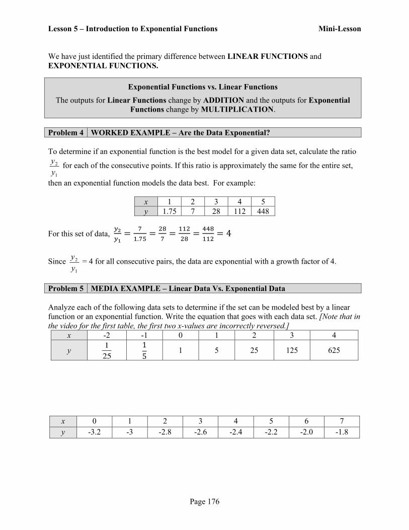
We have just identified the primary difference between LINEAR FUNCTIONS and EXPONENTIAL FUNCTIONS.

Exponential Functions vs. Linear Functions

The outputs for Linear Functions change by ADDITION and the outputs for Exponential Functions change by MULTIPLICATION.

Problem 4 WORKED EXAMPLE – Are the Data Exponential? To determine if an exponential function is the best model for a given data set, calculate the ratio

1

2

yy for each of the consecutive points. If this ratio is approximately the same for the entire set,

then an exponential function models the data best. For example:

x 1 2 3 4 5 y 1.75 7 28 112 448

For this set of data,

!!!!= !

!.!"= !"

!= !!"

!"= !!"

!!"= 4

Since 1

2

yy = 4 for all consecutive pairs, the data are exponential with a growth factor of 4.

Problem 5 MEDIA EXAMPLE – Linear Data Vs. Exponential Data Analyze each of the following data sets to determine if the set can be modeled best by a linear function or an exponential function. Write the equation that goes with each data set. [Note that in the video for the first table, the first two x-values are incorrectly reversed.]

x -2 -1 0 1 2 3 4

y 125

15 1 5 25 125 625

x 0 1 2 3 4 5 6 7 y -3.2 -3 -2.8 -2.6 -2.4 -2.2 -2.0 -1.8


Page 177

Problem 6 YOU TRY – Use Common Ratio to Identify Exponential Data a) Given the following table, explain why the data can be best modeled by an exponential

function. Use the idea of common ratio in your response. x 0 1 2 3 4 5 6

f(x) 15 12 9.6 7.68 6.14 4.92 3.93 b) Determine an exponential model f(x) = abx that fits these data. Start by identifying the values of a and b and then write your final result using proper notation. c) Determine f(10). Round to the nearest hundredth. d) Determine f(50). Write your answer as a decimal and in scientific notation.


Page 178

Section 5.2 – Characteristics of Exponential Functions Exponential Functions are of the form f(x) = abx

where a = the INITIAL VALUE

b = the base (b > 0 and b ≠ 1); also called the GROWTH or DECAY FACTOR

Important Characteristics of the EXPONENTIAL FUNCTION f(x) = abx

• x represents the INPUT quantity

• f(x) represents the OUTPUT quantity

• The graph of f(x) is in the shape of the letter “J” with vertical intercept (0, a) and base b (note that b is the same as the COMMON RATIO from previous examples)

• If b >1, the function is an EXPONENTIAL GROWTH function, and the graph INCREASES from left to right

• If 0 < b < 1, the function is an EXPONENTIAL DECAY function, and the graph DECREASES from left to right

• Another way to identify the vertical intercept is to evaluate f(0).

Problem 7 WORKED EXAMPLE – Examples of Exponential Functions a) f(x) = 2(3)x Initial Value, a = 2, Vertical Intercept = (0, 2)

Base, b = 3. f(x) is an exponential GROWTH function since b > 1.

b) g(x) =1523(1.05)x Initial Value, a = 1523, Vertical Intercept = (0, 1523) Base, b = 1.05. g(x) is an exponential GROWTH function since b > 1.

c) h(x) = 256(0.85)x Initial Value, a = 256, Vertical Intercept = (0, 256) Base, b = 0.85. h(x) is an exponential DECAY function since b < 1.

d) k(x) = 32(0.956)x Initial Value, a = 32, Vertical Intercept = (0, 32) Base, b = 0.956. k(x) is an exponential DECAY function since b < 1.


Page 179

Graph of a generic Exponential Growth Function

f(x) = abx, b > 1

• Domain: All Real Numbers • Range: f(x) > 0 • Horizontal Intercept: None • Vertical Intercept: (0, a) • Horizontal Asymptote: y = 0 • Left to right behavior of the function: INCREASING

Graph of a generic Exponential Decay Function

f(x) = abx, 0 < b < 1

• Domain: All Real Numbers • Range: f(x) > 0 • Horizontal Intercept: None • Vertical Intercept: (0, a) • Horizontal Asymptote: y = 0 • Left to right behavior of the function: DECREASING Problem 8 MEDIA EXAMPLE – Characteristics of Exponential Functions Consider the function f(x) = 12(1.45)x

Initial Value (a): ____________

Base (b):_____________

Domain:_____________________________________

Range:______________________________________

Horizontal Intercept: ______________________

Vertical Intercept:_______________________

Horizontal Asymptote: ________________________

Increasing or Decreasing? ______________________


Page 180

Problem 9 YOU TRY – Characteristics of Exponential Functions Complete the table. Start by graphing each function using the indicated viewing window. Sketch what you see on your calculator screen.

f(x) = 335(1.25)x g(x) = 120(0.75)x

Graph

Use Viewing Window: Xmin = -10 Xmax = 10 Ymin = 0

Ymax = 1000

Initial Value (a)?

Base (b)?

Domain? (Use Inequality Notation)

Range? (Use Inequality Notation)

Horizontal Intercept?

Vertical Intercept?

Horizontal Asymptote? (Write the equation)

Increasing or Decreasing?


Page 181

Section 5.3 – Solving Exponential Equations by Graphing

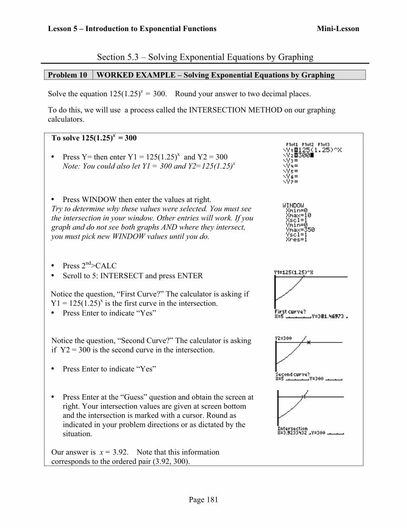
Problem 10 WORKED EXAMPLE – Solving Exponential Equations by Graphing Solve the equation 125(1.25)x = 300. Round your answer to two decimal places. To do this, we will use a process called the INTERSECTION METHOD on our graphing calculators. To solve 125(1.25)x = 300 • Press Y= then enter Y1 = 125(1.25)x and Y2 = 300

Note: You could also let Y1 = 300 and Y2=125(1.25)x

• Press WINDOW then enter the values at right. Try to determine why these values were selected. You must see the intersection in your window. Other entries will work. If you graph and do not see both graphs AND where they intersect, you must pick new WINDOW values until you do.

• Press 2nd>CALC • Scroll to 5: INTERSECT and press ENTER

Notice the question, “First Curve?” The calculator is asking if Y1 = 125(1.25)x is the first curve in the intersection. • Press Enter to indicate “Yes”

Notice the question, “Second Curve?” The calculator is asking if Y2 = 300 is the second curve in the intersection. • Press Enter to indicate “Yes”

• Press Enter at the “Guess” question and obtain the screen at right. Your intersection values are given at screen bottom and the intersection is marked with a cursor. Round as indicated in your problem directions or as dictated by the situation.

Our answer is x = 3.92. Note that this information corresponds to the ordered pair (3.92, 300).


Page 182

Problem 11 WORKED EXAMPLE – Solving Exponential Equations by Graphing Given f(x) = 125(1.25)x find x when f(x) = 50. Round your respond to two decimal places. To do this, we need to SOLVE the equation 125(1.25)x = 50 using the INTERSECTION METHOD. To solve 125(1.25)x = 50

• Press Y= then enter Y1 = 125(1.25)x and Y2 = 50 Note: You could also let Y1 = 50 and Y2=125(1.25)x

• Press WINDOW then enter the values at right. Try to determine why these values were selected. You must see the intersection in your window. Other entries will work. If you graph and do not see both graphs AND where they intersect, you must pick new WINDOW values until you do.

• Press 2nd>CALC • Scroll to 5: INTERSECT and press ENTER

Notice the question, “First Curve?” The calculator is asking if Y1 = 125(1.25)x is the first curve in the intersection.

• Press Enter to indicate “Yes”

Notice the question, “Second Curve?” The calculator is asking if Y2 = 50 is the second curve in the intersection.

• Press Enter to indicate “Yes”

• Press Enter at the “Guess” question and obtain the screen at right. Your intersection values are given at screen bottom and the intersection is marked with a cursor. Round as indicated in your problem directions or as dictated by the situation.

For this problem, we were asked to find x when f(x) = 50. Round to two decimal places. Our response is that, “When f(x) = 50, x = -4.11”. Note that this information corresponds to the ordered pair (-4.11, 50) on the graph of f(x) = 125(1.25)x


Page 183

GUIDELINES FOR SELECTING WINDOW VALUES FOR INTERSECTIONS

While the steps for using the INTERSECTION method are straightforward, choosing values for your window are not always easy. Here are some guidelines for choosing the edges of your window:

• First and foremost, the intersection of the equations MUST appear clearly in the window you select. Try to avoid intersections that appear just on the window’s edges, as these are hard to see and your calculator will often not process them correctly.

• Second, you want to be sure that other important parts of the graphs appear (i.e. where the graph or graphs cross the y-axis or the x-axis).

• When choosing values for x, start with the standard XMin = -10 and Xmax = 10 UNLESS the problem is a real-world problem. In that case, start with Xmin=0 as negative values for a world problem are usually not important. If the values for Xmax need to be increased, choose 25, then 50, then 100 until the intersection of graphs is visible.

• When choosing values for y, start with Ymin = 0 unless negative values of Y are needed for some reason. For Ymax, all graphs need to appear on the screen. So, if solving something like 234(1.23)x = 1000, then choose Ymax to be bigger than 1000 (say, 1500).

If the intersection does not appear in the window, then try to change only one window setting at a time so you can clearly identify the effect of that change (i.e. make Xmax bigger OR change Ymax but not both at once). Try to think about the functions you are working with and what they look like and use a systematic approach to making changes. Problem 12 MEDIA EXAMPLE – Solving Exponential Equations by Graphing Solve the equation 400 = 95(0.89)x . Round your answer to two decimal places.


Page 184

Problem 13 YOU TRY – Window Values and Intersections

In each situation below, you will need to graph to find the solution to the equation using the INTERSECTION method described in this lesson. Fill in the missing information for each situation. Include a rough but accurate sketch of the graphs and intersection point. Mark and label the intersection. Round answers to two decimal places. a) Solve 54(1.05)x = 250 Solution: x = ______________

Xmin:__________ Xmax:__________ Ymin:__________ Ymax:__________

b) Solve 2340(0.82)x = 1250 Solution: x = ______________


c) Solve 45 = 250(1.045)x Solution: x = ______________



Page 185

Section 5.4 – Applications of Exponential Functions

Writing Exponential Equations/Functions Given a set of data that can be modeled using an exponential equation, use the steps below to determine the particulars of the equation:

1. Identify the initial value. This is the a part of the exponential equation y = abx. To find a, look for the starting value of the data set (the output that goes with input 0).

2. Identify the common ratio, b, value. To do this, make a fraction of two consecutive outputs (as long as the inputs are separated by exactly 1). We write this as the fraction

to indicate that we put the second y on top and the first on the bottom. Simplify this

fraction and round as the problem indicates to obtain the value of b. 3. Plug in the values of a and b into y = abx to write the exponential equation.

4. Replace y with appropriate notation as needed to identify a requested exponential FUNCTION.

Problem 14 MEDIA EXAMPLE – Writing Exponential Equations/Functions The population of a small city is shown in the following table.

Year Population 2000 12,545 2001 15,269 2002 18,584

Assume that the growth is exponential. Let t = 0 represent the year 2000. Let a be the initial population in 2000. Let b equal the ratio in population between the years 2000 and 2001. a) Write the equation of the exponential model for this situation. Round any decimals to two

places. Be sure your final result uses proper function notation. b) Using this model, forecast the population in 2008 (to the nearest person). c) Also using this model, determine the nearest whole year in which the population will reach

50,000.

!

y 2y1


Page 186

Problem 15 YOU TRY – Writing Exponential Equations/Functions You have just purchased a new car. The table below shows the value, V, of the car after n years.

n = number of years V = Value of Car 0 24,800 1 21,328 2 18,342

a) Assume that the depreciation is exponential. Write the equation of the exponential model for this situation. Round any decimals to two places. Be sure your final result uses proper function notation.

b) You finance the car for 60 months. What will the value of the car be when the loan is paid

off? Show all steps. Write your answer in a complete sentence. Problem 16 YOU TRY – Writing Exponential Equations/Functions

In 2010, the population of Gilbert, AZ was about 208,000. By 2011, the population had grown to about 215,000.

a) Assuming that the growth is exponential, construct an exponential model that expresses the population, P, of Gilbert, AZ x years since 2010. Your answer must be written in function notation. Round to three decimals as needed.

b) Use this model to predict the population of Gilbert, AZ in 2014. Write your answer in a complete sentence.

c) According to this model, in what year will the population of Gilbert, AZ reach 300,000? (Round your answer DOWN to the nearest whole year.)


Page 187

Problem 17 YOU TRY – Applications of Exponential Functions One 8-oz cup of coffee contains about 100 mg of caffeine. The function A(x) = 100(0.88)

x gives the amount of caffeine (in mg) remaining in the body x hours after drinking a cup of coffee. Answer in complete sentences.

a) Identify the vertical intercept of this function. Write it as an ordered pair and interpret its

meaning in a complete sentence.

b) How much caffeine remains in the body 8 hours after drinking a cup of coffee? Round your

answer to two decimal places as needed. c) How long will it take the body to metabolize half of the caffeine from one cup of coffee?

(i.e. How long until only 50mg of caffeine remain in the body?) Show all of your work, and write your answer in a complete sentence. Round your answer to two decimal places as needed.

d) According to this model, how long will it take for all of the caffeine to leave the

body?


Page 188

Documents

Lesson 5 – Introduction to Exponential Functions · PDF file · 2014-06-122014-06-12 · Lesson 5 – Introduction to Exponential Functions ... $1000 to start + $1000 per day Option