Lesson 4: Signal transmission & Noise

P. Piot, PHYS 375 – Spring 2008

Lesson 4: Signal transmission & Noise

• Signal Transmission– Coupling scheme– Transmission line– Termination & impedance matching

• Noise– White noise– Pink noise– Lock-in amplifier: measuring modulated signal buried into

noise


Signal transmission

• There is often a need to propagate a signal over long distance

• This is accomplished with a transmission line in electronics

• Fancier system convert electronic signal into an optical pulses and use fiber to propagate signal over very long distance (e.g. communication cable under Atlantic ocean)

• The fundamental questions are:– How do we “inject” a signal into a transmission line– How do we model the effect of long transmission line on the

electrical signal– How do we “terminate” the transmission line to get an handle

on the signal and avoid reflections and/or interferences


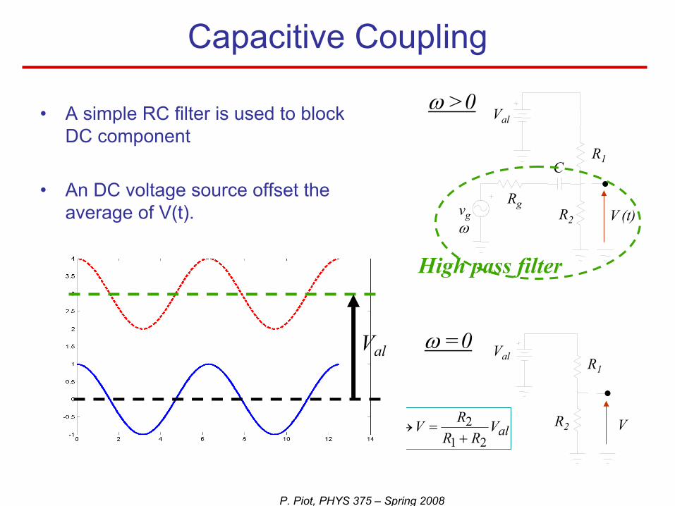
• A simple RC filter is used to block DC component

• An DC voltage source offset the average of V(t).

Capacitive Coupling

V (t)vgω

Rg

Val

R1

R2

C

V

Val R1

R2alVRR

RV21

2+

=→

ω =0

ω >0

High pass filter

Val


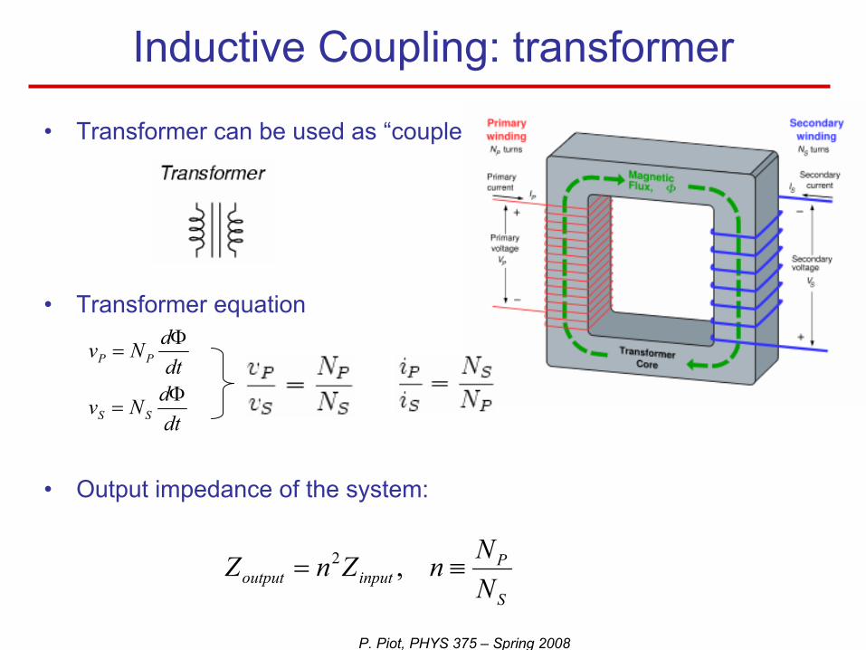
• Transformer can be used as “couplers”

• Transformer equation

• Output impedance of the system:

Inductive Coupling: transformer

dtdNv

dtdNv

SS

PP

Φ=

Φ=

S

Pinputoutput N

NnZnZ ≡= ,2


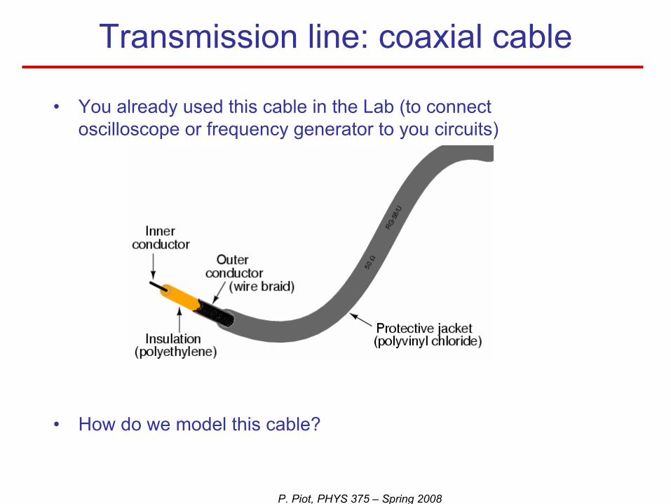
Transmission line: coaxial cable

• You already used this cable in the Lab (to connect oscilloscope or frequency generator to you circuits)

• How do we model this cable?


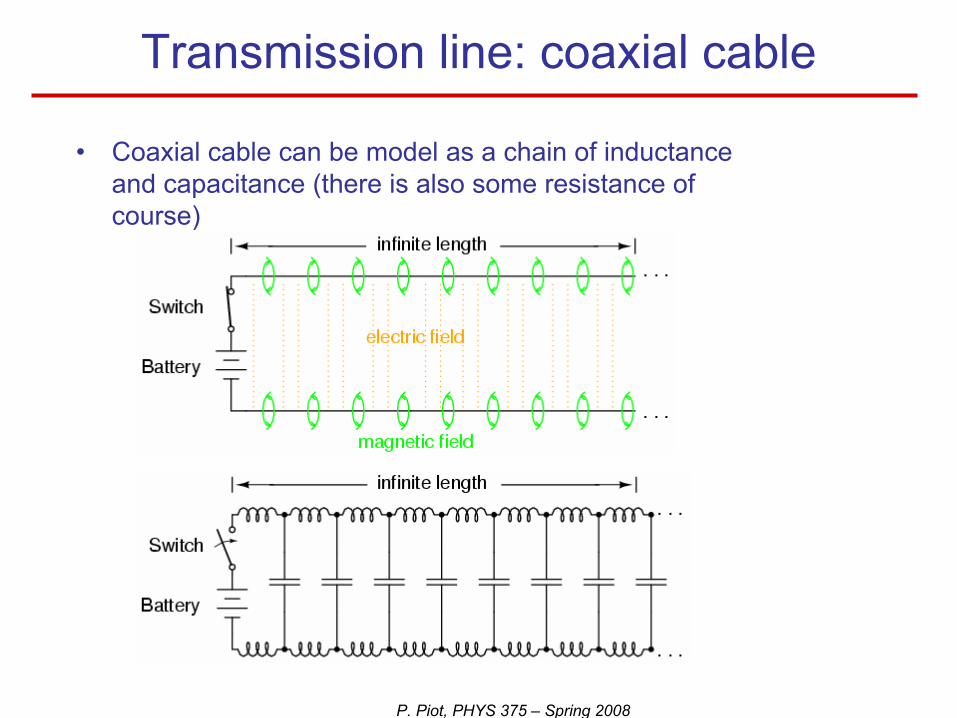
Transmission line: coaxial cable

• Coaxial cable can be model as a chain of inductance and capacitance (there is also some resistance of course)


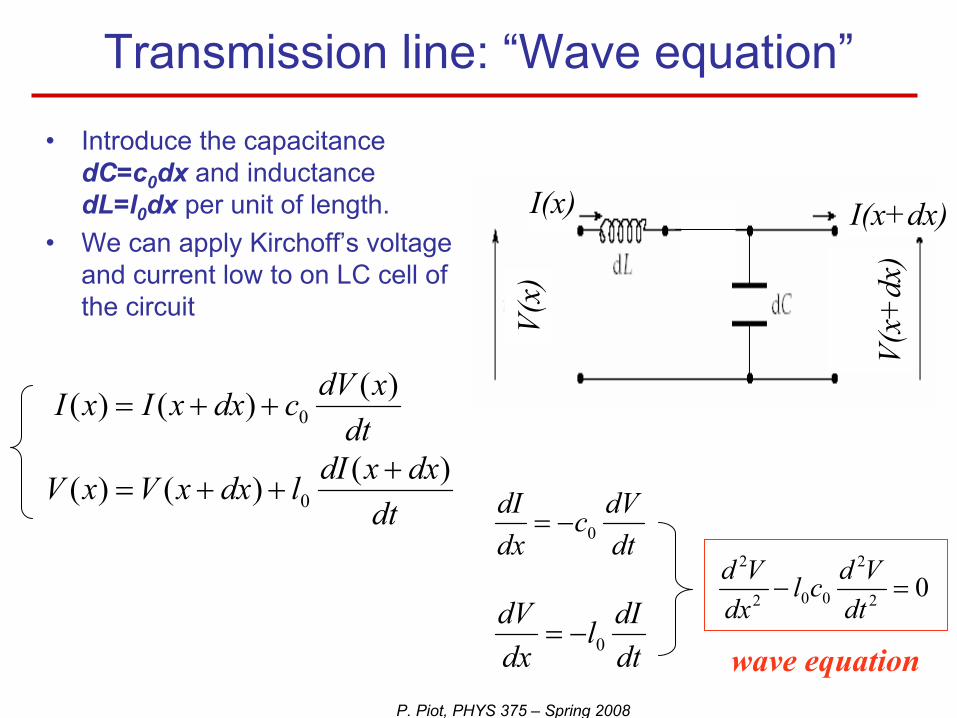
• Introduce the capacitance dC=c0dx and inductance dL=l0dx per unit of length.

• We can apply Kirchoff’s voltage and current low to on LC cell of the circuit

Transmission line: “Wave equation”

02

2

002

2

=−dt

Vdcldx

VddtdVc

dxdI

0−=

dtxdVcdxxIxI )()()( 0++=

dtdIl

dxdV

0−=

dtdxxdIldxxVxV )()()( 0

+++=

I(x) I(x+dx)

V(x)

V(x+

dx)

wave equation


• So the wave equation is satisfied by both I and V

• This are wave equations (in electromagnetism both scalar and vector potentials associated to an e.m. wave obey this equation)

• The l0c0 quantity has the dimension [L-2.T2]:

• The solution of the wave equation are of the form:

Solution of wave equation

][),(

),()(

1)(

0

)(1

)(0

kxtikxti

kxtikxti

eIeIZtxV

eIeItxI+−

+−

−=

+=ωω

ωω

00

1cl

v ≡

02

2

002

2

=

−

I

Vdtdcl

IV

dxd

Forward TWBackward TW


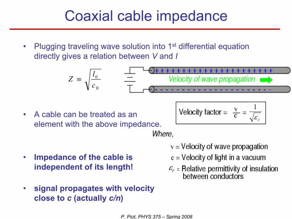
• Plugging traveling wave solution into 1st differential equation directly gives a relation between V and I

• A cable can be treated as an element with the above impedance.

• Impedance of the cable is independent of its length!

• signal propagates with velocity close to c (actually c/n)

Coaxial cable impedance

0

0

clZ ≡

εr

εr

rε1


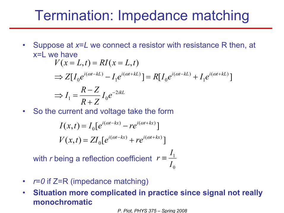
• Suppose at x=L we connect a resistor with resistance R then, at x=L we have

• So the current and voltage take the form

with r being a reflection coefficient

• r=0 if Z=R (impedance matching)• Situation more complicated in practice since signal not really

monochromatic

Termination: Impedance matching

ikL

kLtikLtikLtikLti

eIZRZRI

eIeIReIeIZtLxRItLxV

201

)(1

)(0

)(1

)(0 ][][

),(),(

−

+−+−

+−

=⇒

+=−⇒

===ωωωω

0

1

IIr ≡

][),(

][),()()(

0

)()(0

kxtikxti

kxtikxti

reeZItxV

reeItxI+−

+−

+=

−=ωω

ωω


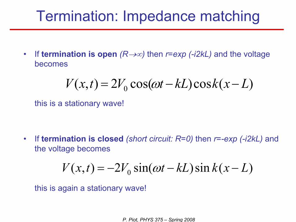
• If termination is open (R→∞) then r=exp (-i2kL) and the voltage becomes

this is a stationary wave!

• If termination is closed (short circuit: R=0) then r=-exp (-i2kL) and the voltage becomes

this is again a stationary wave!

Termination: Impedance matching

)(cos)cos(2),( 0 LxkkLtVtxV −−= ω

)(sin)sin(2),( 0 LxkkLtVtxV −−−= ω


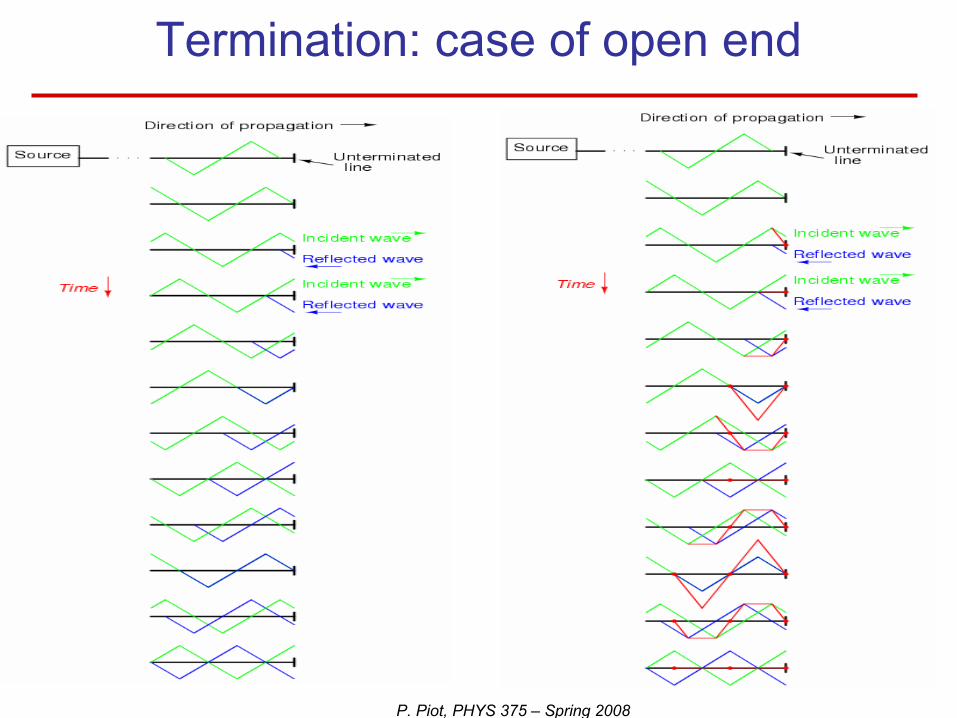
Termination: case of open end


Termination: case of open end (CNT’D)

• Combination of a forward and backward traveling wave yields a standing wave:SIGNAL DOES NOT PROPAGATE

This is a standing waveas one would find in a

resonant electromagnetic cavity


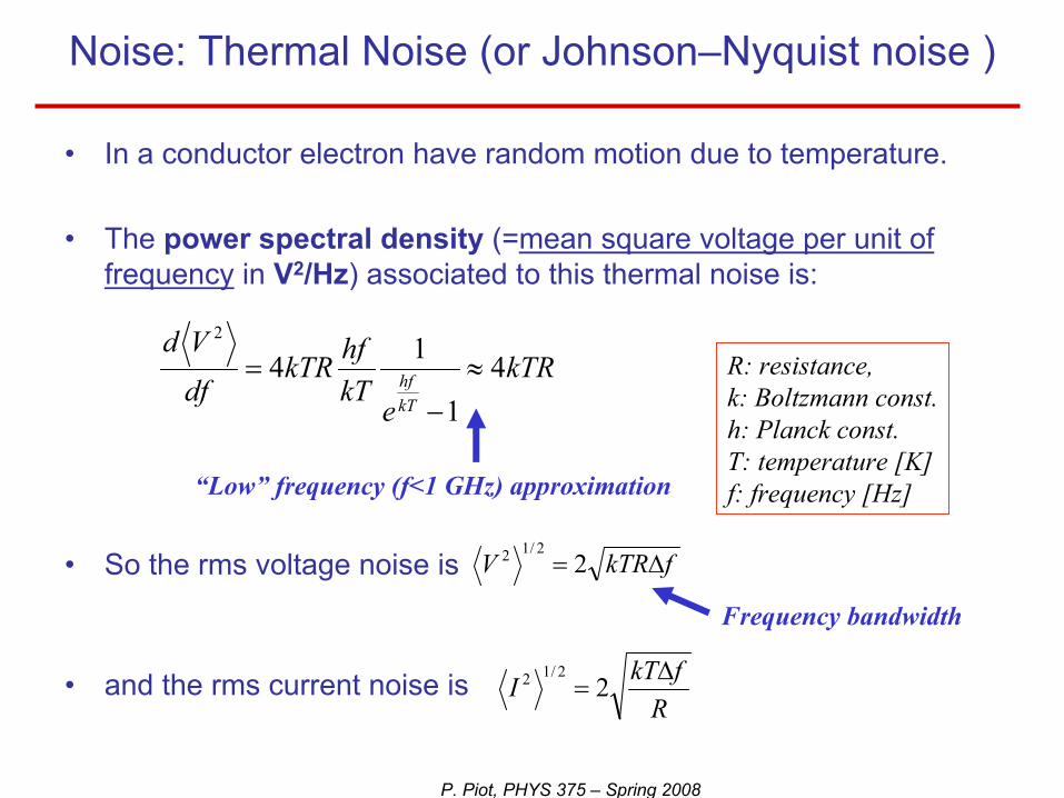
• In a conductor electron have random motion due to temperature.

• The power spectral density (=mean square voltage per unit of frequency in V2/Hz) associated to this thermal noise is:

• So the rms voltage noise is

• and the rms current noise is

Noise: Thermal Noise (or Johnson–Nyquist noise )

kTRe

kThfkTR

dfVd

kThf 41

142

≈−

=

RfkTI ∆

= 22/12

Frequency bandwidth

R: resistance, k: Boltzmann const.h: Planck const.T: temperature [K]f: frequency [Hz]

fkTRV ∆= 22/12

“Low” frequency (f<1 GHz) approximation


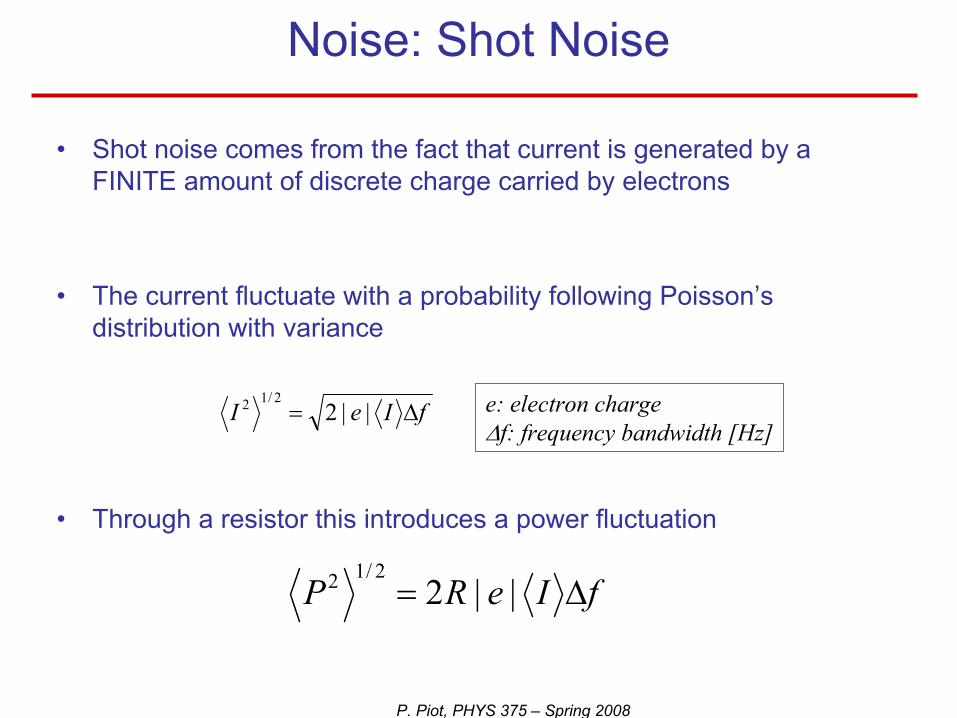
• Shot noise comes from the fact that current is generated by a FINITE amount of discrete charge carried by electrons

• The current fluctuate with a probability following Poisson’s distribution with variance

• Through a resistor this introduces a power fluctuation

Noise: Shot Noise

fIeI ∆= ||22/12 e: electron charge

∆f: frequency bandwidth [Hz]

fIeRP ∆= ||22/12


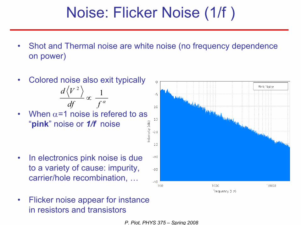
• Shot and Thermal noise are white noise (no frequency dependence on power)

• Colored noise also exit typically

• When α=1 noise is refered to as “pink” noise or 1/f noise

• In electronics pink noise is due to a variety of cause: impurity, carrier/hole recombination, …

• Flicker noise appear for instance in resistors and transistors

Noise: Flicker Noise (1/f )

αfdfVd 1

2

∝


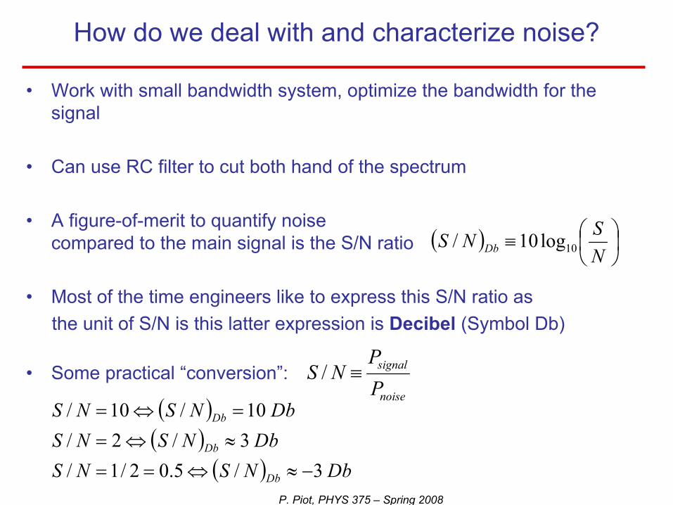
• Work with small bandwidth system, optimize the bandwidth for thesignal

• Can use RC filter to cut both hand of the spectrum

• A figure-of-merit to quantify noise compared to the main signal is the S/N ratio

• Most of the time engineers like to express this S/N ratio asthe unit of S/N is this latter expression is Decibel (Symbol Db)

• Some practical “conversion”:

How do we deal with and characterize noise?

( )( )

( ) DbNSNSDbNSNS

DbNSNS

Db

Db

Db

3/5.02/1/3/2/10/10/

−≈⇔==≈⇔==⇔=

noise

signal

PP

NS ≡/

( )

≡

NSNS Db 10log10/


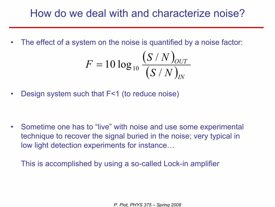
• The effect of a system on the noise is quantified by a noise factor:

• Design system such that F<1 (to reduce noise)

• Sometime one has to “live” with noise and use some experimental technique to recover the signal buried in the noise; very typical in low light detection experiments for instance…

This is accomplished by using a so-called Lock-in amplifier

How do we deal with and characterize noise?

( )( )IN

OUT

NSNSF//log10 10=


Detection of ultra-low signal buried in noise: The lock-in amplifier

)cos()cos(

ϕωω

+=+=

tBBNtAA

)cos(ˆ)]cos()2[cos(2

ˆˆ)cos(ˆ)cos()cos(ˆˆ

ϕωϕϕω

ϕωϕωω

++++=

+++=

tNAtBA

tNAttBAAB

What remains after low pass filter


Lock-in amplifier: a numerical example

Documents

Lesson 4: Signal transmission & Noise