Embed Size (px)
Citation preview
RELATIONSHIPS BETWEEN ELEMENTS OF LESLIE MATRICES AND FUTURE GROWTH OF THE
POPULATION
By
Lorisha Lynn Riley
Honors Capstone Project
Submitted to the Faculty of
Olivet Nazarene University
for partial fulfillment of the requirements for
GRADUATION WITH UNIVERSITY HONORS
March, 2014
BACHELOR OF SCIENCE
in
Mathematics
Capstone Project Advisor (printed) Signature Date
Honors Council Chair (printed) Signature Date
Honors Council Member (printed) Signature Date

ii
ACKNOWLEDGEMENTS
This project would not have been possible without the selfless support of the Olivet
Nazarene University mathematics faculty, including Dr. Justin Brown, Dr. Dale Hathaway, Dr.
David Atkinson, Dr. Nick Boros, and Dr. Daniel Green. I would like to give my thanks to Dr. Justin
Brown for the support and encouragement necessary to bring about the completion of this
project. With the guidance of Dr. Justin Brown, my research mentor, this project has grown into
more than I had hoped. He suggested the topic for my research and supported this research with
his guidance and knowledge. The rest of the faculty not only taught me much of what I know
about mathematics, but also supported me throughout this process. It is their dedication that
has brought me to this point.
I would also like to thank the Olivet Nazarene University Honors Program, which
provided a foundation of academic excellence and monetary support upon which this project
grew. Without their help, this project would not have been nearly as successful.
iii
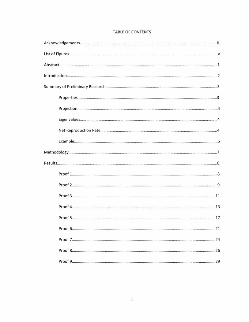
TABLE OF CONTENTS
Acknowledgements…………………………………………………………………………………………………………………….ii
List of Figures……………………………………………………….…………………………….……………………………………….v
Abstract……………………………………………………….………………………………………………………………………….….1
Introduction………………………………………….………………………………………………………………………….…………2
Summary of Preliminary Research…………………………………………….…………………………………..……………3
Properties………………………………………………………………………………………………………………………3
Projection…………………………………………………………………………………………………………….…………4
Eigenvalues…………………………………….………………………………………………………………………………4
Net Reproduction Rate…………………………………………………………………………………………………..4
Example………………………………………………………………….………………………………………………………5
Methodology………………………………………………………………………………………………………………………………7
Results………………………………………………………………………………….…………………………………………………….8
Proof 1……………………………………………………………………………………………………………………………8
Proof 2……………………………………………………………………………………………………………………………9
Proof 3…………………………………………………………………………………………………………………….……11
Proof 4………………………………………………………………………………………………….………………………13
Proof 5…………………………………………………………………………………………………….……………………17
Proof 6……………………………………………………………………………………………………….…………………21
Proof 7………………………………………………………………………………………………………….………………24
Proof 8………………………………………………………………………………………………………….………………26
Proof 9…………………………………………………………………………………………………………….……………29
iv
Discussion…………………………………………………………………………………………………………………………………31
Conclusion…………………………………………………………………….……………………………………………..32
Direction of Further Research………………………………………………………………………………………32
Migration Models…………………………………………………………………………………………………………32
Works Cited……….……………………………………………………………………………….…………………………………….34

v
LIST OF FIGURES
Figure 1: The Leslie Matrix………………………………………………………………………………………………………….3
Figure 2: Leslie Matrix for Dog Population…………………………….…………………………………………………….5
Figure 3: Migration Model…………………………………………………………………………………………………………..5
1
ABSTRACT
Leslie matrices have been used for years to model and predict the growth of animal
populations. Recently, general rules have been applied that can relatively easily determine
whether an animal population will grow or decline. My mentor, Dr. Justin Brown and I examine,
more specifically, whether there are relationships between certain elements of a population and
the dominant eigenvalue, which determines growth. Not only do we consider the general 3x3
Leslie matrix, but also we looked into modified versions for incomplete data and migration
models of Leslie matrices. We successfully found several connections within these cases;
however, there is much more research that could be done.
Keywords: Leslie matrix, migration, eigenvalue, dominant eigenvalue, characteristic equation,
net reproduction rate, population growth
2
INTRODUCTION
Leslie matrices are named for Patrick Holt Leslie (1900-1972), who created them after
researching rodent populations under Charles Elton at Oxford (Bacaër, 2011, p. 117). In 1945,
Leslie published his article in Biometrika detailing his findings concerning population models
(Leslie, 1945, p. 183-212). Leslie matrices are used in mathematical ecology to determine how
populations are affected by characteristics such as survival and fertility rates. Specifically, Leslie
matrices are used in mathematical ecology to predict how populations of animals grow or
decline. Using formulas, the eigenvalues of the Leslie matrices are found, including the dominant
eigenvalue (see section labeled “Eigenvalue” for definition). If the dominant eigenvalue and,
hence, all the eigenvalues are less than 1, then the population will decline. If the dominant
eigenvalue is greater than one, regardless of the values of the other eigenvalues, the population
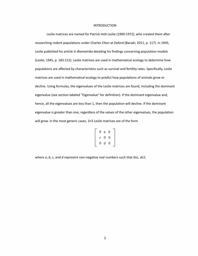
will grow. In the most generic cases, 3×3 Leslie matrices are of the form
0 a b
c 0 0
0 d 0
where a, b, c, and d represent non-negative real numbers such that 0≤c, d≤1.
3
SUMMARY OF PRELIMINARY RESEARCH
Suppose there is a population of dogs divided into three age classes- young, middle
aged, and old. It is also known that each dog will progress into the next age class in one time
period (Burks, Lindquist, & McMurran, 2008, p. 76). If we know the survival and fertility rates for
each age class, it is then possible to deduce a number of characteristics about this population
using Leslie matrices.
Properties
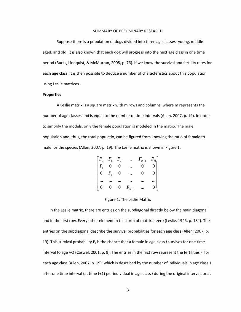
A Leslie matrix is a square matrix with m rows and columns, where m represents the
number of age classes and is equal to the number of time intervals (Allen, 2007, p. 19). In order
to simplify the models, only the female population is modeled in the matrix. The male
population and, thus, the total populatio, can be figured from knowing the ratio of female to
male for the species (Allen, 2007, p. 19). The Leslie matrix is shown in Figure 1.
0...000
..................
00...00
00...00
...
1
2
1
1210
m
mm
P
P
P
FFFFF
Figure 1: The Leslie Matrix
In the Leslie matrix, there are entries on the subdiagonal directly below the main diagonal
and in the first row. Every other element in this form of matrix is zero (Leslie, 1945, p. 184). The
entries on the subdiagonal describe the survival probabilities for each age class (Allen, 2007, p.
19). This survival probability Pi is the chance that a female in age class i survives for one time
interval to age i+1 (Caswel, 2001, p. 9). The entries in the first row represent the fertilities Fi for
each age class (Allen, 2007, p. 19), which is described by the number of individuals in age class 1
after one time interval (at time t+1) per individual in age class i during the original interval, or at
4
time t (Caswell, 2001, p. 10). Lastly, the initial state population vector is a vector where each
entry represents the number of individuals in each age group at time t. (Caswell, 2001, p. 10;
Leslie, 1945, p. 183). Thus t+1 is the age class one interval after the original time.
Projection
Knowing the properties of the Leslie matrix listed above and the initial population, it is
possible to project the population. To begin, the initial population values are placed into a
vector. This is then multiplied by the Leslie matrix that is raised to the power of the number of
time intervals projected (Allen, 2007, p. 19). Projection is expressed using the formula
X(t)=LtX(0), where X(t) is the projection matrix, t is the desired number of time intervals of
projection, and X(0) is the initial population vector.
Eigenvalues
Eigenvalues are one of the more important properties to consider when looking at Leslie
matrices because they give an idea of how the population will change over time. To find
eigenvalues, the characteristic equation det(A-λI)=0 is solved for lambda. In other words,
subtract λ times the identity matrix I from the original matrix A, then find the determinant and
set this equal to 0. For each Leslie matrix, there will then be a dominant eigenvalue that has a
value greater than the absolute value of any other eigenvalue (Anton & Rorres, 1994, p. 759).
The value of the eigenvalue describes the change in population in the future- if ǀλǀ is less than
one, the population will decrease and if ǀλǀ is greater than one, the population will increase.
Net Reproduction Rate
Net reproduction rate is another statistic that can be found using the Leslie matrix. The
net reproduction rate is simply the expected number of children a female will bear during her
lifetime by taking the sum of each survival probability multiplied by all previous fertility rates.
This rate is represented by the expression
5
R=F0+F1P1+F2P1P2+…+FNP1P2…Pn-1.
This shows that a population has zero value population growth if and only if its net reproduction
rate is 1 (Anton & Rorres, 1994, p.763).
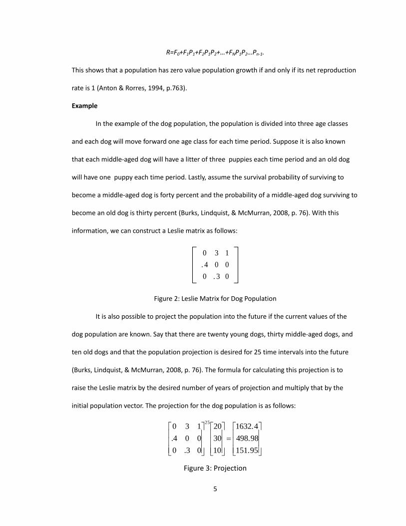
Example
In the example of the dog population, the population is divided into three age classes
and each dog will move forward one age class for each time period. Suppose it is also known
that each middle-aged dog will have a litter of three puppies each time period and an old dog
will have one puppy each time period. Lastly, assume the survival probability of surviving to
become a middle-aged dog is forty percent and the probability of a middle-aged dog surviving to
become an old dog is thirty percent (Burks, Lindquist, & McMurran, 2008, p. 76). With this
information, we can construct a Leslie matrix as follows:
0 3 1
. 4 0 0
0 . 3 0
Figure 2: Leslie Matrix for Dog Population
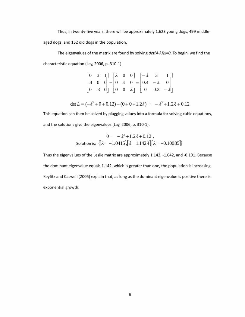
It is also possible to project the population into the future if the current values of the
dog population are known. Say that there are twenty young dogs, thirty middle-aged dogs, and
ten old dogs and that the population projection is desired for 25 time intervals into the future
(Burks, Lindquist, & McMurran, 2008, p. 76). The formula for calculating this projection is to
raise the Leslie matrix by the desired number of years of projection and multiply that by the
initial population vector. The projection for the dog population is as follows:
95.151
98.498
4.1632
10
30
20
03.0
004.
13025
Figure 3: Projection
6
Thus, in twenty-five years, there will be approximately 1,623 young dogs, 499 middle-
aged dogs, and 152 old dogs in the population.
The eigenvalues of the matrix are found by solving det(A-λI)x=0. To begin, we find the
characteristic equation (Lay, 2006, p. 310-1).
3.00
04.0
13
00
00
00
03.0
004.
130
)2.100()12.00(det 3 L 12.02.13
This equation can then be solved by plugging values into a formula for solving cubic equations,
and the solutions give the eigenvalues (Lay, 2006, p. 310-1).
0 12.02.13 ,
Solution is: 85100.0,4142.1,5041.1
Thus the eigenvalues of the Leslie matrix are approximately 1.142, -1.042, and -0.101. Because
the dominant eigenvalue equals 1.142, which is greater than one, the population is increasing.
Keyfitz and Caswell (2005) explain that, as long as the dominant eigenvalue is positive there is
exponential growth.
7
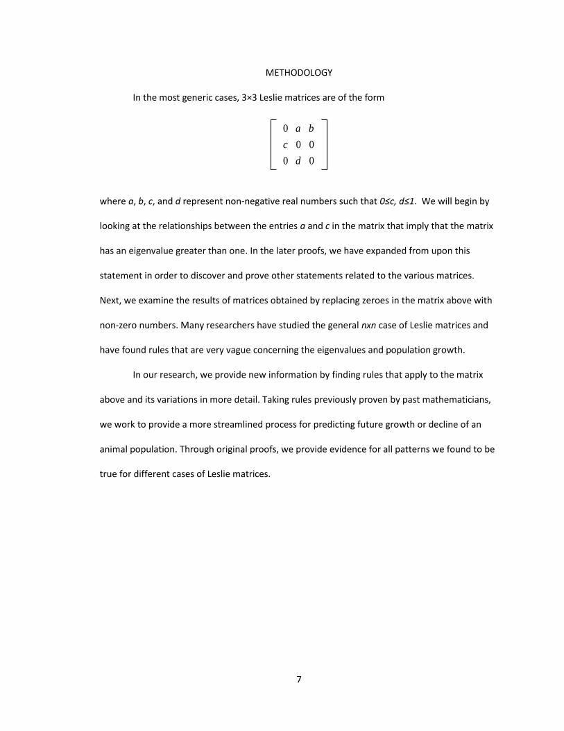
METHODOLOGY
In the most generic cases, 3×3 Leslie matrices are of the form
0 a b
c 0 0
0 d 0
where a, b, c, and d represent non-negative real numbers such that 0≤c, d≤1. We will begin by
looking at the relationships between the entries a and c in the matrix that imply that the matrix
has an eigenvalue greater than one. In the later proofs, we have expanded from upon this
statement in order to discover and prove other statements related to the various matrices.
Next, we examine the results of matrices obtained by replacing zeroes in the matrix above with
non-zero numbers. Many researchers have studied the general nxn case of Leslie matrices and
have found rules that are very vague concerning the eigenvalues and population growth.
In our research, we provide new information by finding rules that apply to the matrix
above and its variations in more detail. Taking rules previously proven by past mathematicians,
we work to provide a more streamlined process for predicting future growth or decline of an
animal population. Through original proofs, we provide evidence for all patterns we found to be
true for different cases of Leslie matrices.
8
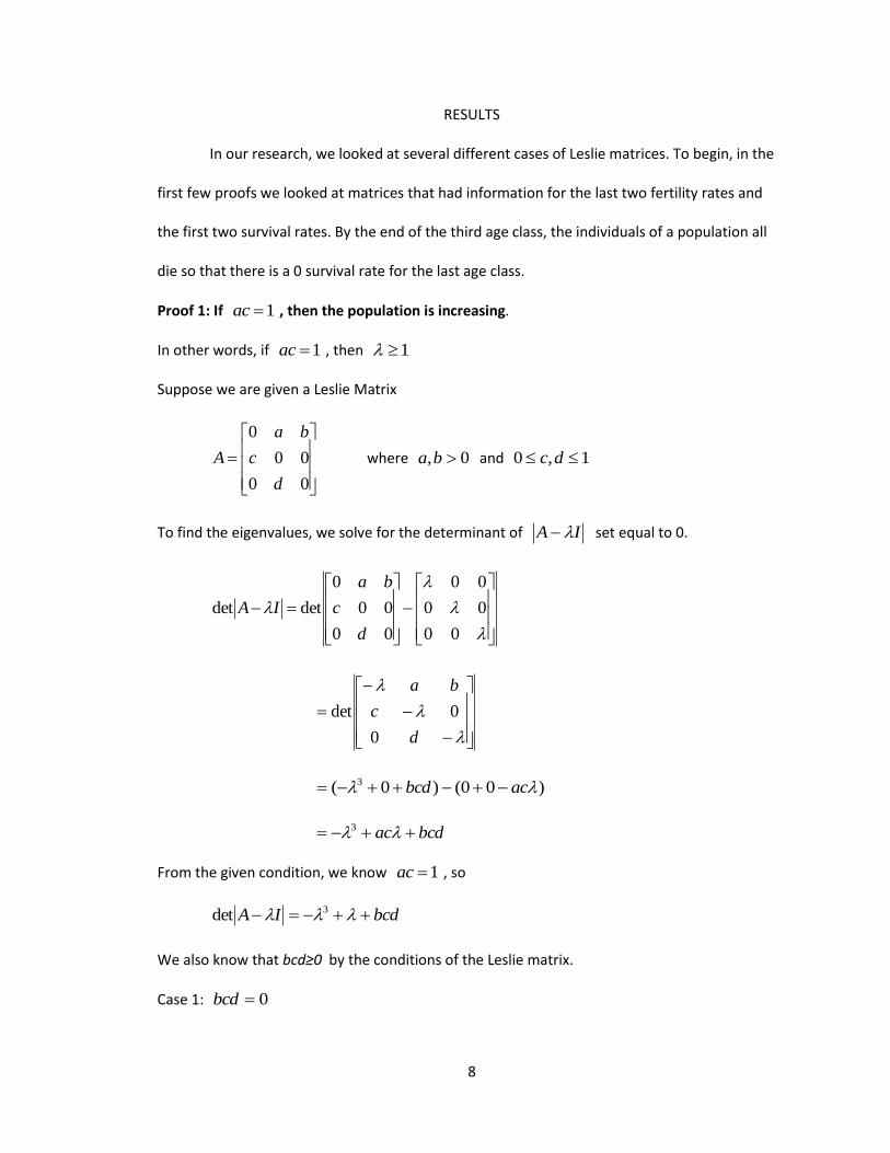
RESULTS
In our research, we looked at several different cases of Leslie matrices. To begin, in the
first few proofs we looked at matrices that had information for the last two fertility rates and
the first two survival rates. By the end of the third age class, the individuals of a population all
die so that there is a 0 survival rate for the last age class.
Proof 1: If 1ac , then the population is increasing.
In other words, if 1ac , then 1
Suppose we are given a Leslie Matrix
00
00
0
d
c
ba
A where 0, ba and 1,0 dc
To find the eigenvalues, we solve for the determinant of IA set equal to 0.
00
00
00
00
00
0
detdet
d
c
ba
IA
d
c
ba
0
0det
)00()0( 3 acbcd
bcdac 3
From the given condition, we know 1ac , so
bcdIA 3det
We also know that bcd≥0 by the conditions of the Leslie matrix.
Case 1: 0bcd
9
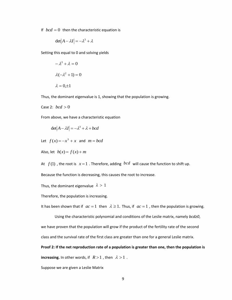
If 0bcd then the characteristic equation is
3det IA
Setting this equal to 0 and solving yields
03
0)1( 2
1,0
Thus, the dominant eigenvalue is 1, showing that the population is growing.
Case 2: 0bcd
From above, we have a characteristic equation
bcdIA 3det
Let xxxf 3)( and bcdm
Also, let mxfxh )()(
At )1(f , the root is 1x . Therefore, adding bcd will cause the function to shift up.
Because the function is decreasing, this causes the root to increase.
Thus, the dominant eigenvalue 1
Therefore, the population is increasing.
It has been shown that if 1ac then .1 Thus, if 1ac , then the population is growing.
Using the characteristic polynomial and conditions of the Leslie matrix, namely bcd≥0,
we have proven that the population will grow if the product of the fertility rate of the second
class and the survival rate of the first class are greater than one for a general Leslie matrix.
Proof 2: If the net reproduction rate of a population is greater than one, then the population is
increasing. In other words, if 1R , then 1 .
Suppose we are given a Leslie Matrix
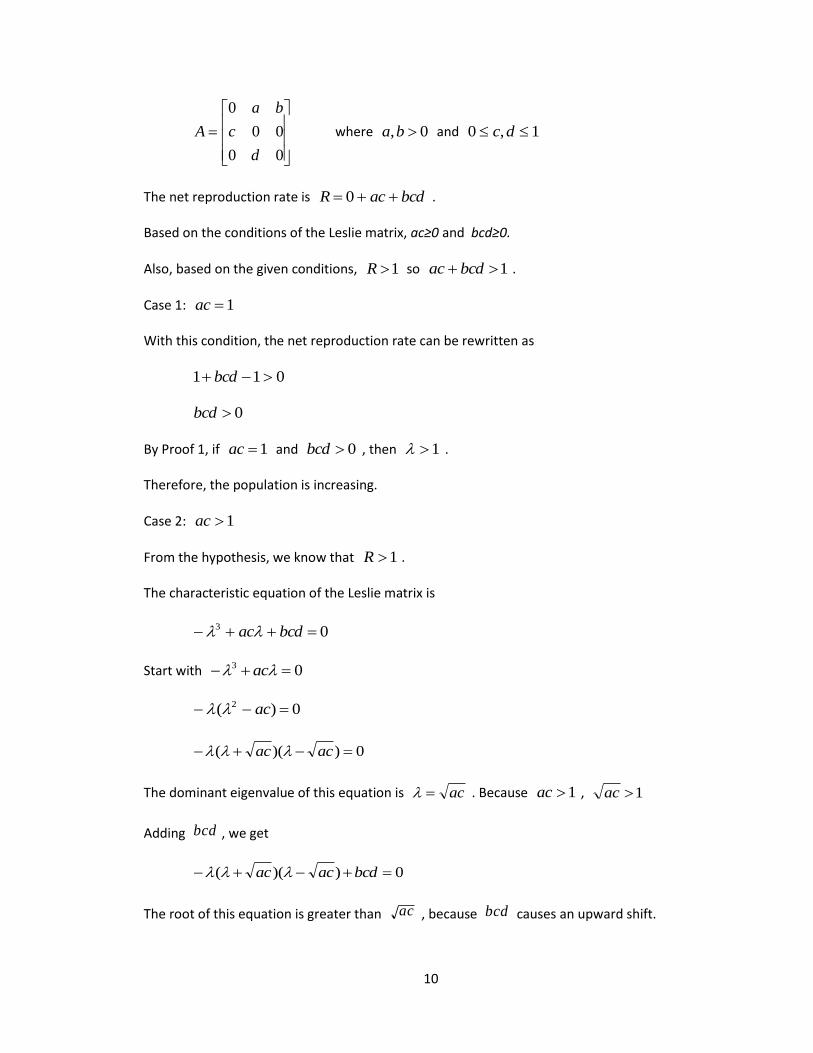
10
00
00
0
d
c
ba
A where 0, ba and 1,0 dc
The net reproduction rate is bcdacR 0 .
Based on the conditions of the Leslie matrix, ac≥0 and bcd≥0.
Also, based on the given conditions, 1R so 1 bcdac .
Case 1: 1ac
With this condition, the net reproduction rate can be rewritten as
011 bcd
0bcd
By Proof 1, if 1ac and 0bcd , then 1 .
Therefore, the population is increasing.
Case 2: 1ac
From the hypothesis, we know that 1R .
The characteristic equation of the Leslie matrix is
03 bcdac
Start with 03 ac
0)( 2 ac
0))(( acac
The dominant eigenvalue of this equation is ac . Because 1ac , 1ac
Adding bcd , we get
0))(( bcdacac
The root of this equation is greater than ac , because bcd causes an upward shift.
11
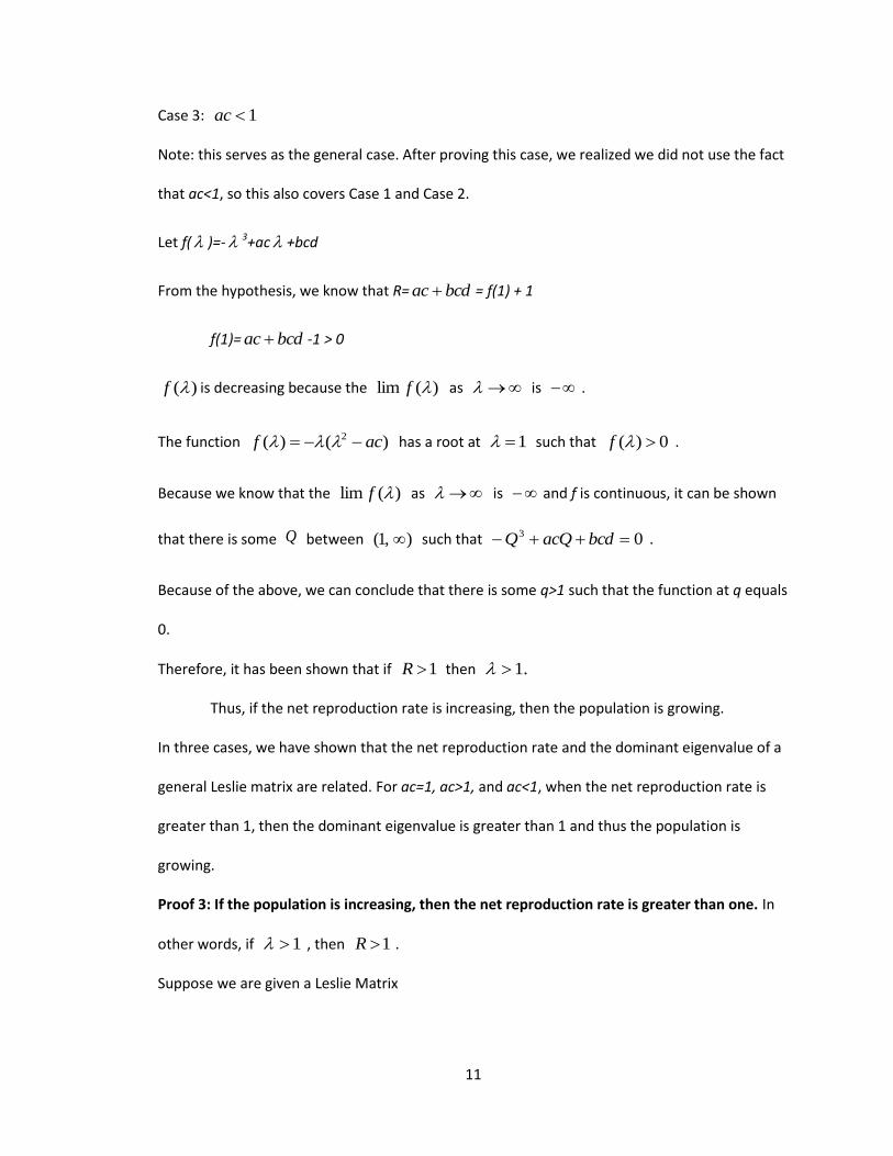
Case 3: 1ac
Note: this serves as the general case. After proving this case, we realized we did not use the fact
that ac<1, so this also covers Case 1 and Case 2.
Let f( )=- 3+ac +bcd
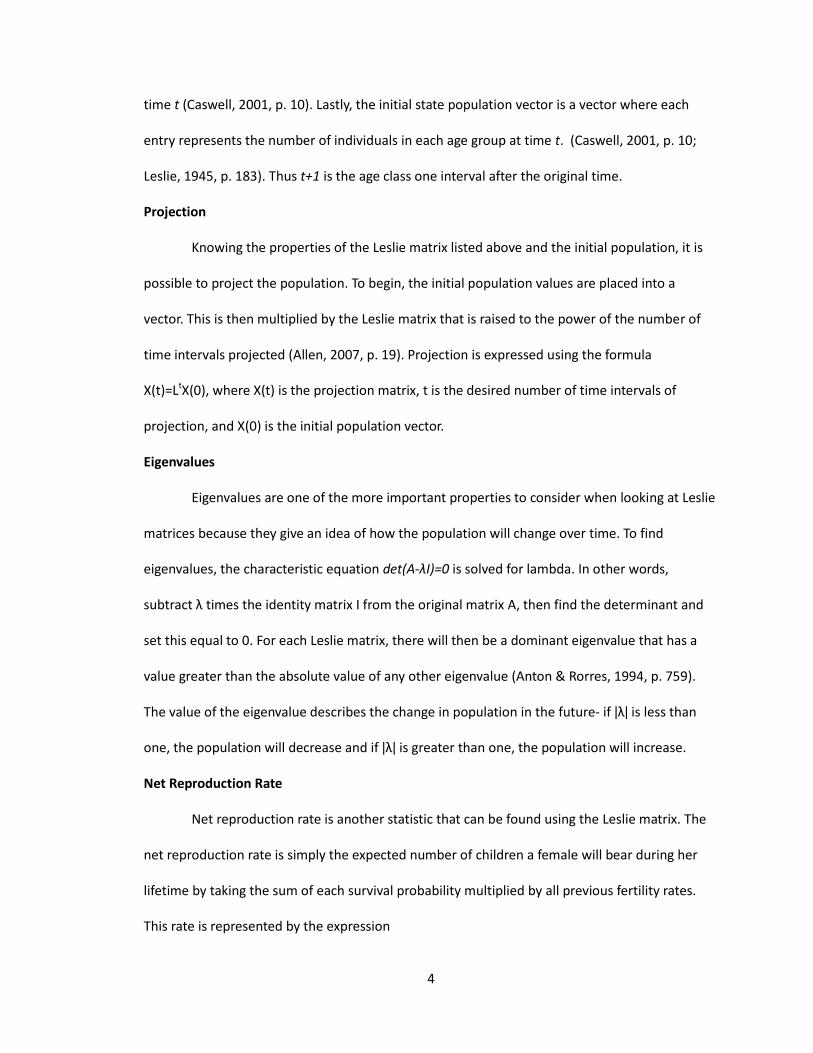
From the hypothesis, we know that R= bcdac = f(1) + 1
f(1)= bcdac -1 > 0
)(f is decreasing because the )(lim f as is .
The function )()( 2 acf has a root at 1 such that 0)( f .
Because we know that the )(lim f as is and f is continuous, it can be shown
that there is some Q between ,1( ) such that 03 bcdacQQ .
Because of the above, we can conclude that there is some q>1 such that the function at q equals
0.
Therefore, it has been shown that if 1R then .1
Thus, if the net reproduction rate is increasing, then the population is growing.
In three cases, we have shown that the net reproduction rate and the dominant eigenvalue of a
general Leslie matrix are related. For ac=1, ac>1, and ac<1, when the net reproduction rate is
greater than 1, then the dominant eigenvalue is greater than 1 and thus the population is
growing.
Proof 3: If the population is increasing, then the net reproduction rate is greater than one. In
other words, if 1 , then 1R .
Suppose we are given a Leslie Matrix
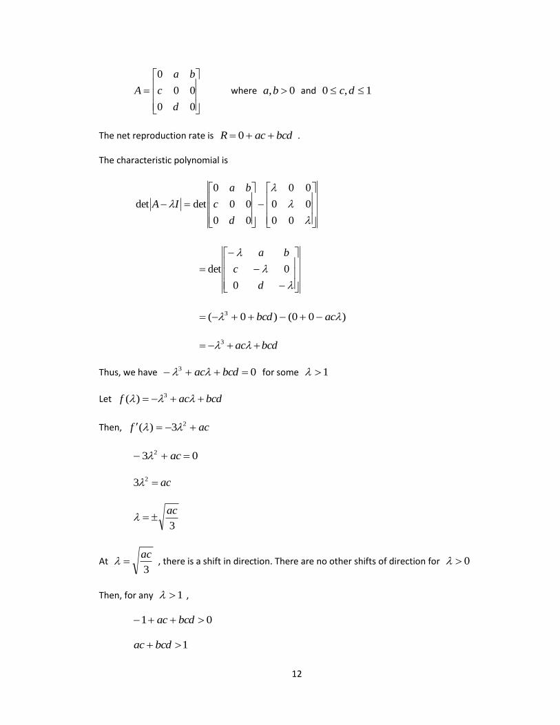
12
00
00
0
d
c
ba
A where 0, ba and 1,0 dc
The net reproduction rate is bcdacR 0 .
The characteristic polynomial is
00
00
00
00
00
0
detdet
d
c
ba
IA
d
c
ba
0
0det
)00()0( 3 acbcd
bcdac 3
Thus, we have 03 bcdac for some 1
Let bcdacf 3)(
Then, acf 23)(
03 2 ac
ac23
3
ac
At 3
ac , there is a shift in direction. There are no other shifts of direction for 0
Then, for any 1 ,
01 bcdac
1 bcdac
13
Therefore, it has been shown that if 1 then .1R
Thus, if the population is increasing, then the net reproduction rate is greater than one.
In a general Leslie matrix, we have proven that if the population is growing, indicated by
a dominant eigenvalue greater than 1, then the net reproduction rate is also greater than 1. This
was shown by looking at the graphical representation of the characteristic equation and the
shifts it undergoes.
Therefore, it can be said that the net reproduction rate is greater than one if and only if
the population is increasing. In other words, 1R if and only if 1 .
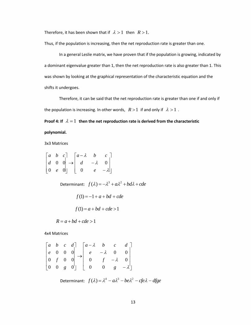
Proof 4: If 1 then the net reproduction rate is derived from the characteristic
polynomial.
3x3 Matrices
e
d
cba
e
d
cba
0
0
00
00
Determinant: cdebdaf 23)(
cdebdaf 1)1(
1)1( cdebdaf
1 cdebdaR
4x4 Matrices
g
f
e
dcba
g
f
e
dcba
00
00
00
000
000
000
Determinant: dfgecfebeaf 234)(
14
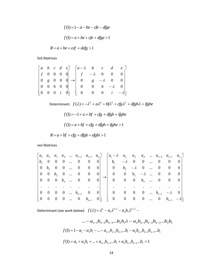
dfgecfebeaf 1)1(
1)1( dfgecfebeaf
1 defgcefbeaR
5x5 Matrices
i
h
g
f
edcba
i
h
g
f
edcba
000
000
000
000
0000
0000
0000
0000
Determinant: ifghedfghcfgbfaf 2345)(
ifghedfghcfgbfaf 1)1(
1)1( ifghedfghcfgbfaf
1 efghidfghcfgbfaR
nxn Matrices
1
2
4
3
2
1
124321
1
2
4
3
2
1
124321
0...0000
0...0000
........
000...000
000...00
000...00
000...00
...
00...0000
00...0000
........
000...000
000...000
000...000
000...000
...
n
n
nnn
n
n
nnn
b
b
b
b
b
b
aaaaaaa
b
b
b
b
b
b
aaaaaaa
Determinant (see work below): 2
12
1
1)( nnn baaf
13211321121 .........1)1( bbbbabbbabaaf nnnnnnn
1.........)1( 121121121 bbbabbabaaf nnnnn
1232112321 ......... bbbbbabbbba nnnnnnn
15
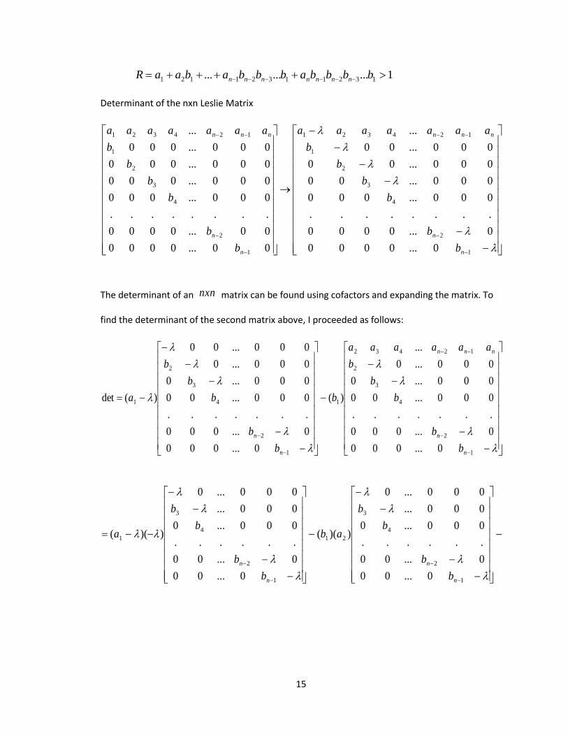
1......... 13211321121 bbbbabbbabaaR nnnnnnn
Determinant of the nxn Leslie Matrix
1
2
4
3
2
1
124321
1
2
4
3
2
1
124321
0...0000
0...0000
........
000...000
000...00
000...00
000...00
...
00...0000
00...0000
........
000...000
000...000
000...000
000...000
...
n
n
nnn
n
n
nnn
b
b
b
b
b
b
aaaaaaa
b
b
b
b
b
b
aaaaaaa
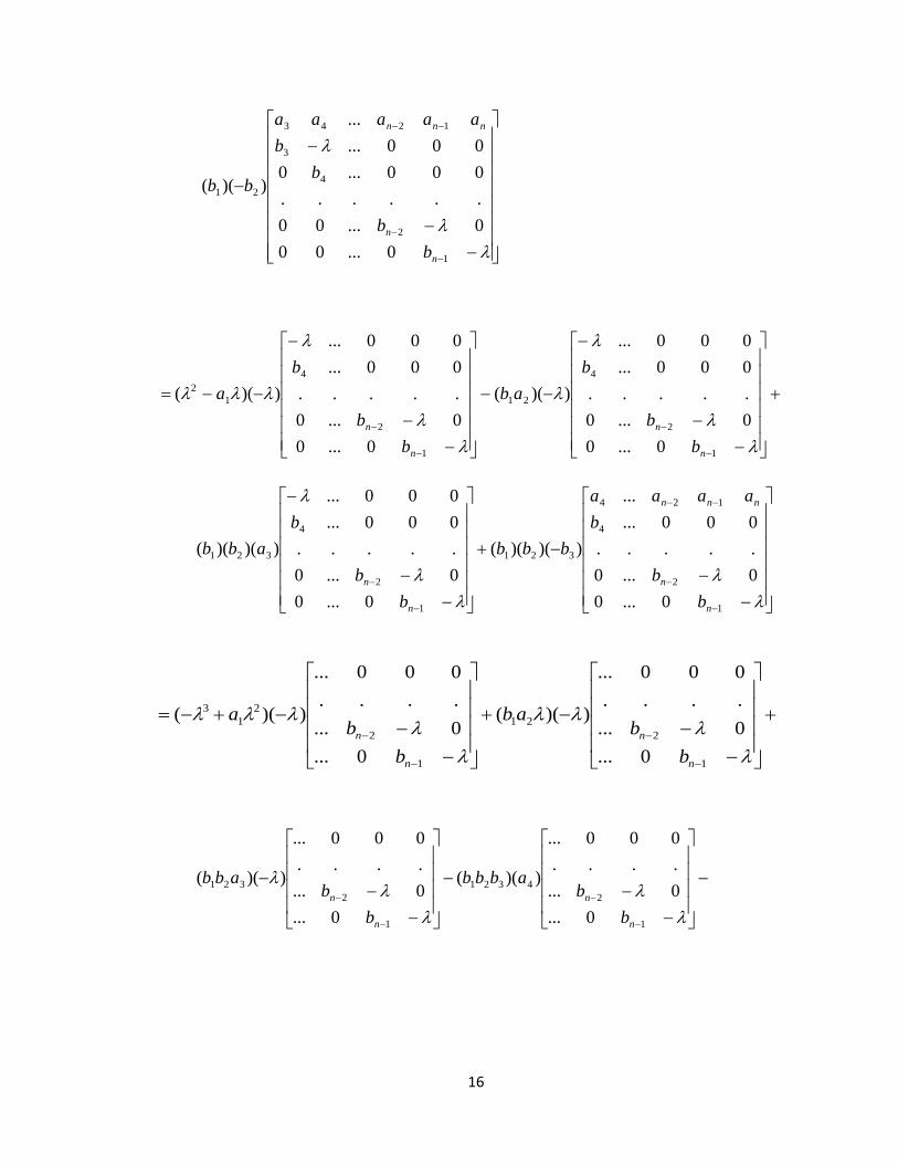
The determinant of an nxn matrix can be found using cofactors and expanding the matrix. To
find the determinant of the second matrix above, I proceeded as follows:
1
2
4
3
2
12432
1
1
2
4
3
2
1
0...000
0...000
.......
000...00
000...0
000...0
...
)(
0...000
0...000
.......
000...00
000...0
000...0
000...00
)(det
n
n
nnn
n
n
b
b
b
b
b
aaaaaa
b
b
b
b
b
b
a
1
2
4
3
21
1
2
4
3
1
0...00
0...00
......
000...0
000...
000...0
))((
0...00
0...00
......
000...0
000...
000...0
))((
n
n
n
n
b
b
b
b
ab
b
b
b
b
a
16
1
2
4
3
1243
21
0...00
0...00
......
000...0
000...
...
))((
n
n
nnn
b
b
b
b
aaaaa
bb
1
2
4
21
1
2
4
1
2
0...0
0...0
.....
000...
000...
))((
0...0
0...0
.....
000...
000...
))((
n
n
n
n
b
b
b
ab
b
b
b
a
1
2
4
124
321
1
2
4
321
0...0
0...0
.....
000...
...
))()((
0...0
0...0
.....
000...
000...
))()((
n
n
nnn
n
n
b
b
b
aaaa
bbb
b
b
b
abb
1
2
4321
1
2
321
0...
0...
....
000...
))((
0...
0...
....
000...
))((
n
n
n
n
b
babbb
b
babb
1
2
21
1
2
2
1
3
0...
0...
....
000...
))((
0...
0...
....
000...
))((
n
n
n
n
b
bab
b
ba
17
1
2
12
4321
0...
0...
....
...
))((
n
n
nnn
b
b
aaa
bbbb
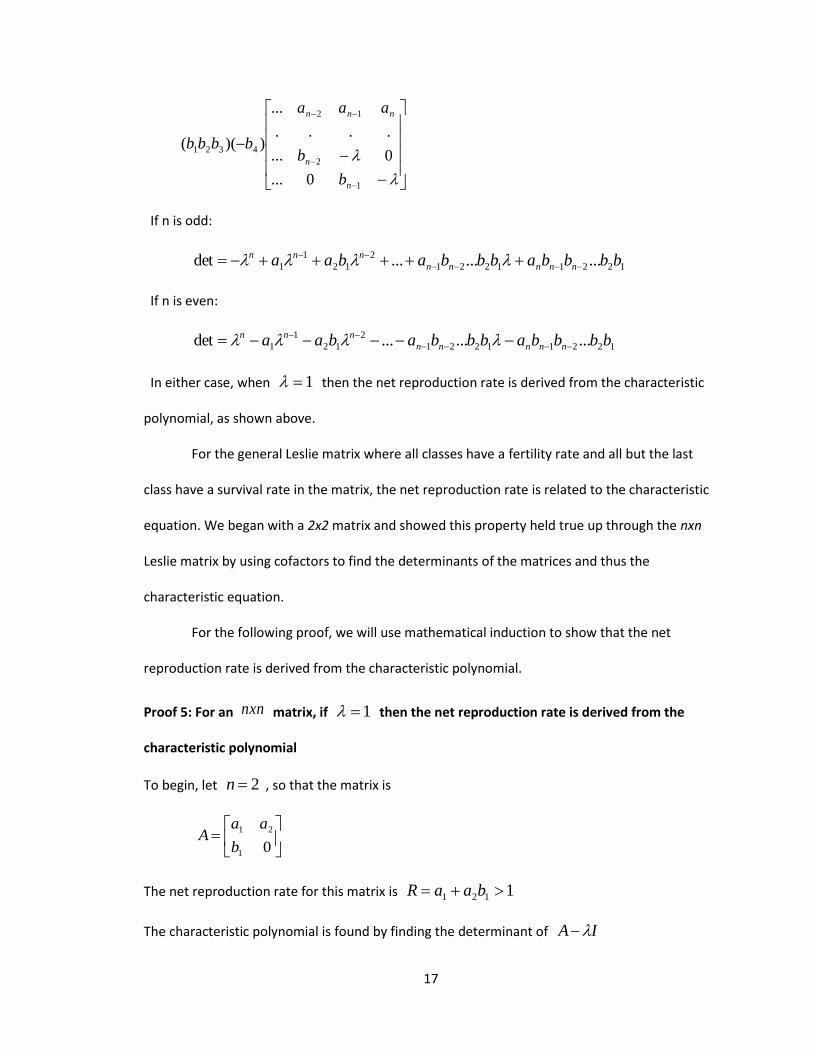
If n is odd:
12211221
2
12
1
1 .........det bbbbabbbabaa nnnnn
nnn
If n is even:
12211221
2
12
1
1 .........det bbbbabbbabaa nnnnn
nnn
In either case, when 1 then the net reproduction rate is derived from the characteristic
polynomial, as shown above.
For the general Leslie matrix where all classes have a fertility rate and all but the last
class have a survival rate in the matrix, the net reproduction rate is related to the characteristic
equation. We began with a 2x2 matrix and showed this property held true up through the nxn
Leslie matrix by using cofactors to find the determinants of the matrices and thus the
characteristic equation.
For the following proof, we will use mathematical induction to show that the net
reproduction rate is derived from the characteristic polynomial.
Proof 5: For an nxn matrix, if 1 then the net reproduction rate is derived from the
characteristic polynomial
To begin, let 2n , so that the matrix is
01
21
b
aaA
The net reproduction rate for this matrix is 1121 baaR
The characteristic polynomial is found by finding the determinant of IA

18
1
21detdet
b
aaIA
][)]([ 121 baa
121
2 baa
When 1
1211det baa
1121 baa
The characteristic equation is equal to the net reproduction rate when 1 for a 2n
Assume that this holds for all kn such that the net reproduction rate
1221123121 ...... bbbbabbabaaR kkk
and that the characteristic equation is
1232112321
2
12
1
1 .........det bbbbbabbbbabaa nnnnnnn
nnn
as shown in the earlier examples
Let 1 kn , thus the matrix is
0000...000
0000...000
0000...000
0000...000
...........................
00000...00
00000...00
...
1
2
3
2
1
1123321
k
k
k
k
kkkkk
b
b
b
b
b
b
aaaaaaaa
The net reproduction rate R is
1......... 121112321121 bbbbabbbbbabaaR kkkkkkk
19
k
k
k
k
kkkkk
b
b
b
b
b
b
aaaaaaaa
IA
000...000
000...000
000...000
000...000
...........................
00000...0
00000...0
...
1
2
3
2
1
1123321
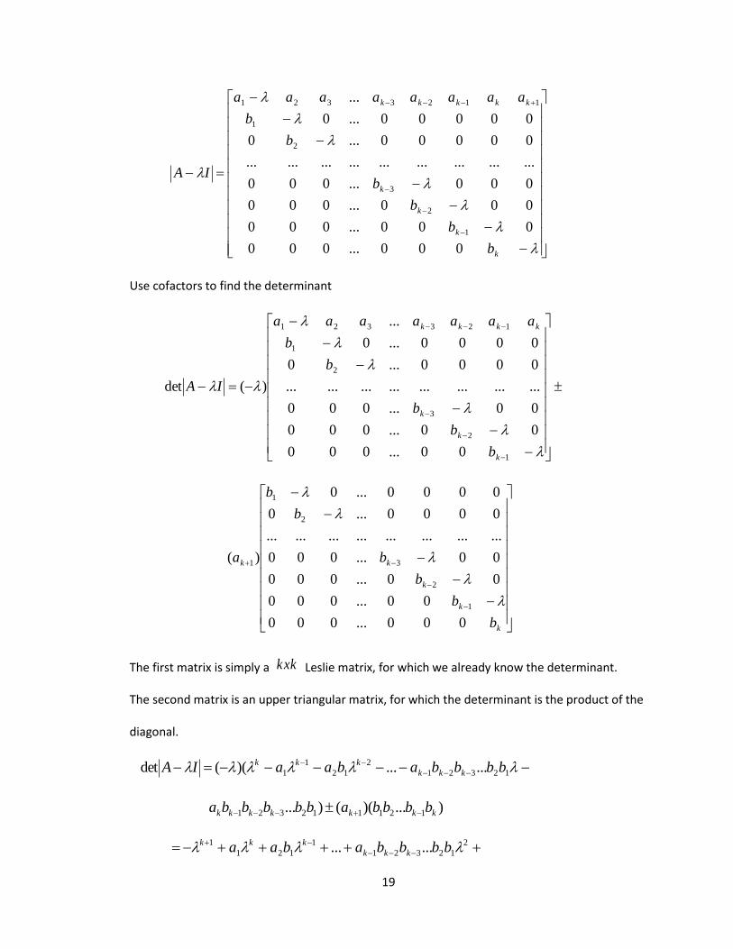
Use cofactors to find the determinant
1
2
3
2
1
123321
00...000
00...000
00...000
........................
0000...0
0000...0
...
)(det
k
k
k
kkkk
b
b
b
b
b
aaaaaaa
IA
k
k
k
kk
b
b
b
b
b
b
a
000...000
00...000
00...000
00...000
........................
0000...0
0000...0
)(
1
2
3
2
1
1
The first matrix is simply a kxk Leslie matrix, for which we already know the determinant.
The second matrix is an upper triangular matrix, for which the determinant is the product of the
diagonal.
12321
2
12
1
1 ......)((det bbbbabaaIA kkk
kkk
)...)(()... 121112321 kkkkkkk bbbbabbbbba
2
12321
1
121
1 ...... bbbbabaa kkk
kkk
20
kkkkkkk bbbbabbbbba 121112321 ......
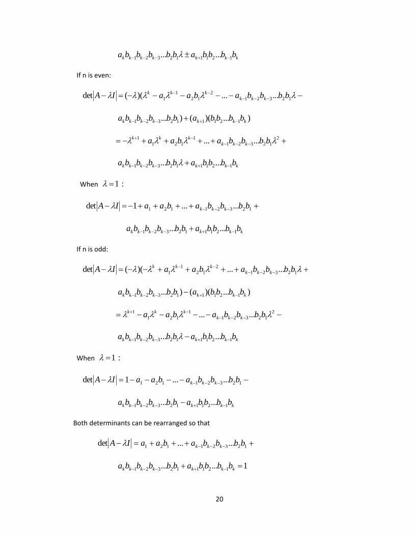
If n is even:
12321
2
12
1
1 ......)((det bbbbabaaIA kkk
kkk
)...)(()... 121112321 kkkkkkk bbbbabbbbba
2
12321
1
121
1 ...... bbbbabaa kkk
kkk
kkkkkkk bbbbabbbbba 121112321 ......
When :1
12321121 ......1det bbbbabaaIA kkk
kkkkkkk bbbbabbbbba 121112321 ......
If n is odd:
12321
2
12
1
1 ......)((det bbbbabaaIA kkk
kkk
)...)(()... 121112321 kkkkkkk bbbbabbbbba
2
12321
1
121
1 ...... bbbbabaa kkk
kkk
kkkkkkk bbbbabbbbba 121112321 ......
When :1
12321121 ......1det bbbbabaaIA kkk
kkkkkkk bbbbabbbbba 121112321 ......
Both determinants can be rearranged so that
12321121 ......det bbbbabaaIA kkk
1...... 121112321 kkkkkkk bbbbabbbbba
21
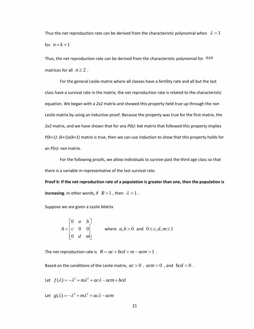
Thus the net reproduction rate can be derived from the characteristic polynomial when 1
for 1 kn
Thus, the net reproduction rate can be derived from the characteristic polynomial for nxn
matrices for all 2n .
For the general Leslie matrix where all classes have a fertility rate and all but the last
class have a survival rate in the matrix, the net reproduction rate is related to the characteristic
equation. We began with a 2x2 matrix and showed this property held true up through the nxn
Leslie matrix by using an inductive proof. Because the property was true for the first matrix, the
2x2 matrix, and we have shown that for any P(k): kxk matrix that followed this property implies
P(k+1): (k+1)x(k+1) matrix is true, then we can use induction to show that this property holds for
an P(n): nxn matrix.
For the following proofs, we allow individuals to survive past the third age class so that
there is a variable m representative of the last survival rate.
Proof 6: If the net reproduction rate of a population is greater than one, then the population is
increasing. In other words, if 1R , then 1 .
Suppose we are given a Leslie Matrix
md
c
ba
A
0
00
0
where 0, ba and 1,,0 mdc
The net reproduction rate is 1 acmmbcdacR .
Based on the conditions of the Leslie matrix, 0ac , 0acm , and 0bcd .
Let bcdacmacmf 23)(
Let acmacmg 23)(
22
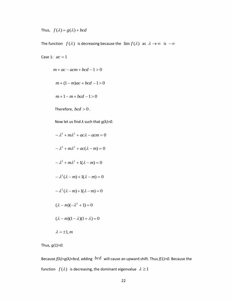
Thus, bcdgf )()(
The function )(f is decreasing because the )(lim f as is
Case 1: 1ac
01 bcdacmacm
01)1( bcdacmm
011 bcdmm
Therefore, 0bcd .
Now let us find λ such that g(λ)=0.
023 acmacm
0)(23 macm
0)(123 mm
0)(1)(2 mm
0)(1)(2 mm
0)1)(( 2 m
0)1)(1)(( m
m,1
Thus, g(1)=0.
Because f(λ)=g(λ)+bcd, adding bcd will cause an upward shift. Thus f(1)>0. Because the
function )(f is decreasing, the dominant eigenvalue 1
23
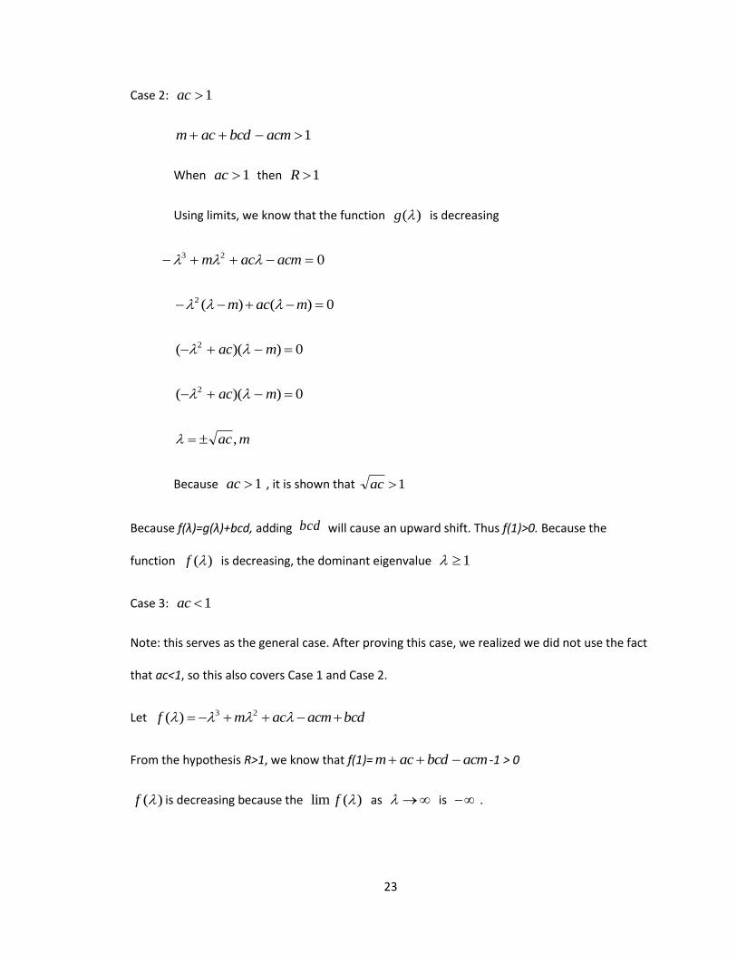
Case 2: 1ac
1 acmbcdacm
When 1ac then 1R
Using limits, we know that the function )(g is decreasing
023 acmacm
0)()(2 macm
0))(( 2 mac
0))(( 2 mac
mac,
Because 1ac , it is shown that 1ac
Because f(λ)=g(λ)+bcd, adding bcd will cause an upward shift. Thus f(1)>0. Because the
function )(f is decreasing, the dominant eigenvalue 1
Case 3: 1ac
Note: this serves as the general case. After proving this case, we realized we did not use the fact
that ac<1, so this also covers Case 1 and Case 2.
Let bcdacmacmf 23)(
From the hypothesis R>1, we know that f(1)= acmbcdacm -1 > 0
)(f is decreasing because the )(lim f as is .
24
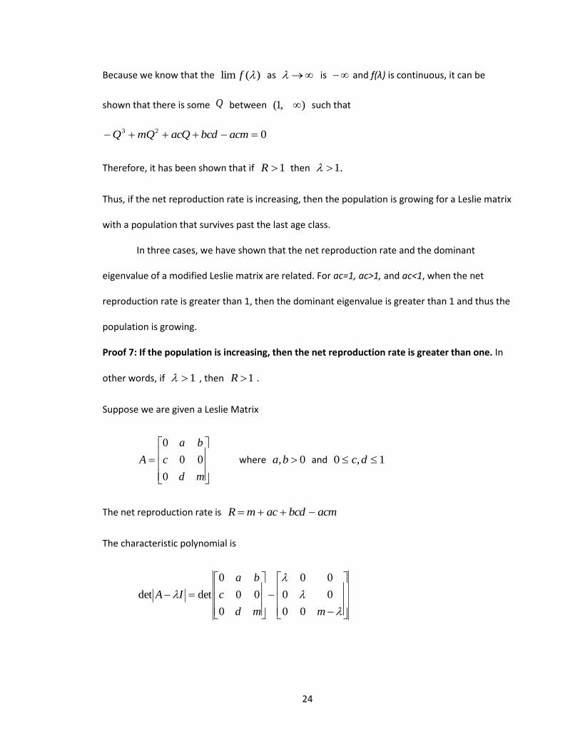
Because we know that the )(lim f as is and f(λ) is continuous, it can be
shown that there is some Q between ,1( ) such that
023 acmbcdacQmQQ
Therefore, it has been shown that if 1R then .1
Thus, if the net reproduction rate is increasing, then the population is growing for a Leslie matrix
with a population that survives past the last age class.
In three cases, we have shown that the net reproduction rate and the dominant
eigenvalue of a modified Leslie matrix are related. For ac=1, ac>1, and ac<1, when the net
reproduction rate is greater than 1, then the dominant eigenvalue is greater than 1 and thus the
population is growing.
Proof 7: If the population is increasing, then the net reproduction rate is greater than one. In
other words, if 1 , then 1R .
Suppose we are given a Leslie Matrix
md
c
ba
A
0
00
0
where 0, ba and 1,0 dc
The net reproduction rate is acmbcdacmR
The characteristic polynomial is
mmd
c
ba
IA
00
00
00
0
00
0
detdet
25
md
c
ba
0
0det
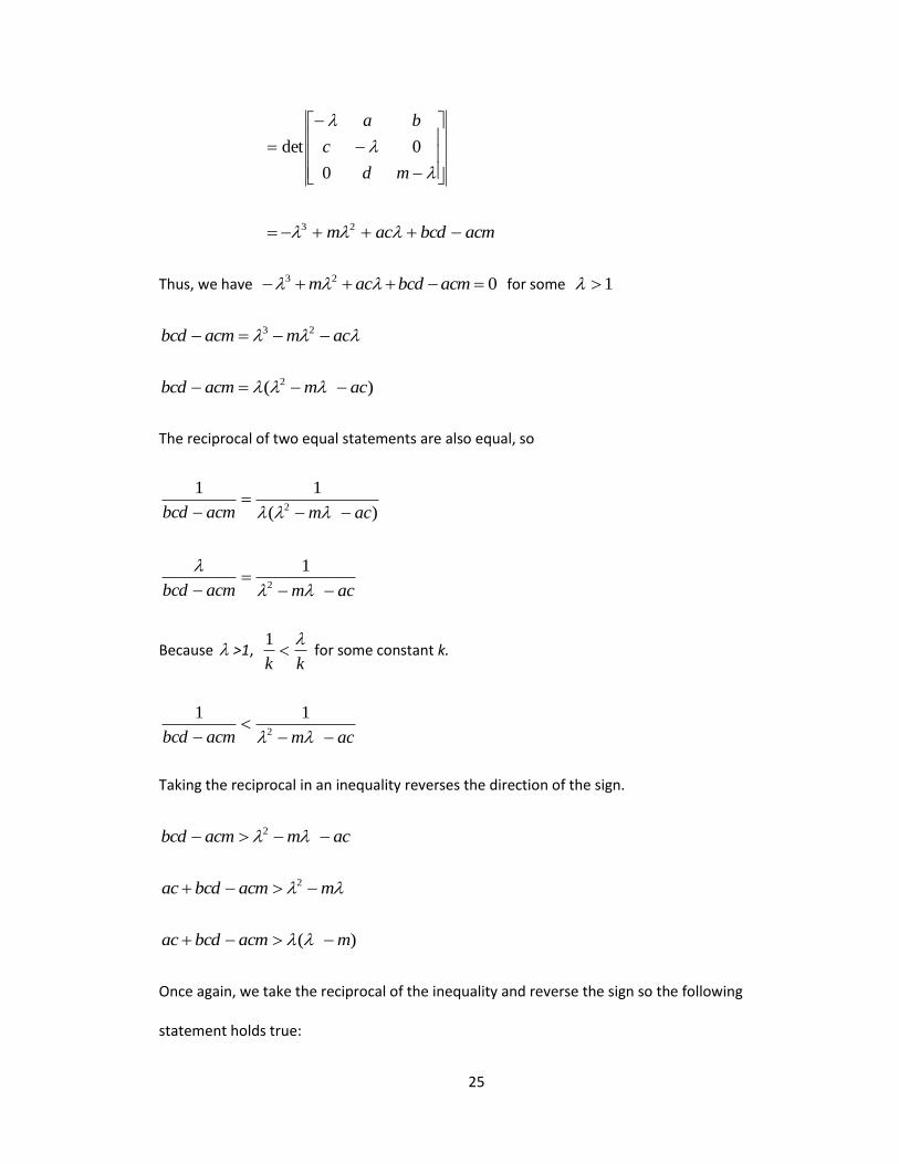
acmbcdacm 23
Thus, we have 023 acmbcdacm for some 1
acmacmbcd 23
)( 2 acmacmbcd
The reciprocal of two equal statements are also equal, so
)(
112 acmacmbcd
acmacmbcd
2
1
Because >1, kk
1 for some constant k.
acmacmbcd
2
11
Taking the reciprocal in an inequality reverses the direction of the sign.
acmacmbcd 2
macmbcdac 2
)( macmbcdac
Once again, we take the reciprocal of the inequality and reverse the sign so the following
statement holds true:
26
)(
11
macmbcdac
macmbcdac
1
macmbcdac
11
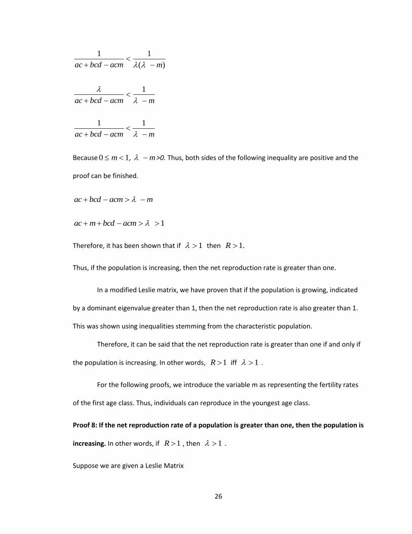
Because 10 m , m >0. Thus, both sides of the following inequality are positive and the
proof can be finished.
macmbcdac
1 acmbcdmac
Therefore, it has been shown that if 1 then .1R
Thus, if the population is increasing, then the net reproduction rate is greater than one.
In a modified Leslie matrix, we have proven that if the population is growing, indicated
by a dominant eigenvalue greater than 1, then the net reproduction rate is also greater than 1.
This was shown using inequalities stemming from the characteristic population.
Therefore, it can be said that the net reproduction rate is greater than one if and only if
the population is increasing. In other words, 1R iff 1 .
For the following proofs, we introduce the variable m as representing the fertility rates
of the first age class. Thus, individuals can reproduce in the youngest age class.
Proof 8: If the net reproduction rate of a population is greater than one, then the population is
increasing. In other words, if 1R , then 1 .
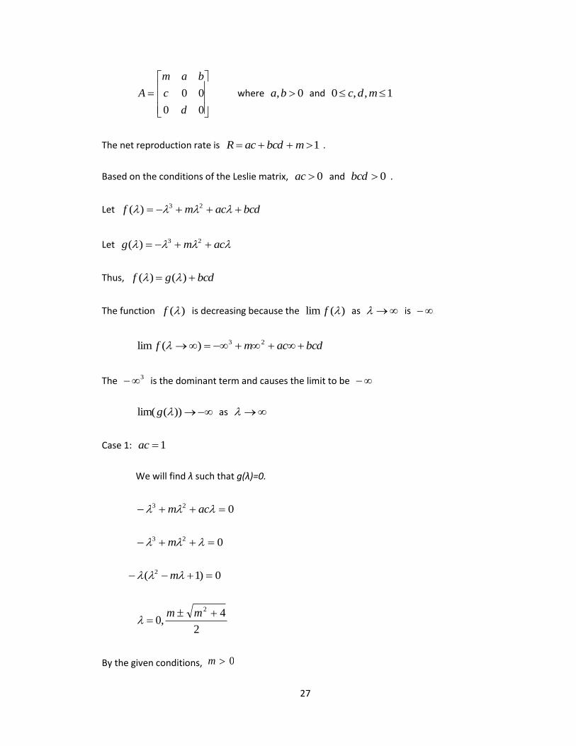
Suppose we are given a Leslie Matrix
27
00
00
d
c
bam
A where 0, ba and 1,,0 mdc
The net reproduction rate is 1 mbcdacR .
Based on the conditions of the Leslie matrix, 0ac and 0bcd .
Let bcdacmf 23)(
Let acmg 23)(
Thus, bcdgf )()(
The function )(f is decreasing because the )(lim f as is
bcdacmf 23)(lim
The 3 is the dominant term and causes the limit to be
))(lim( g as
Case 1: 1ac
We will find λ such that g(λ)=0.
023 acm
023 m
0)1( 2 m
2
4,0
2
mm
By the given conditions, m 0
28
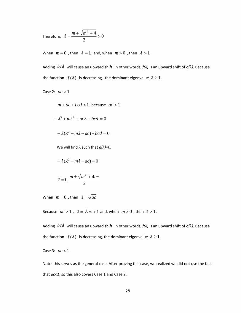
Therefore, 02
42
mm
When 0m , then 1 , and, when 0m , then 1
Adding bcd will cause an upward shift. In other words, f(λ) is an upward shift of g(λ). Because
the function )(f is decreasing, the dominant eigenvalue 1 .
Case 2: 1ac
1 bcdacm because 1ac
023 bcdacm
0)( 2 bcdacm
We will find λ such that g(λ)=0.
0)( 2 acm
2
4,0
2 acmm
When 0m , then ac
Because 1ac , 1 ac and, when 0m , then 1 .
Adding bcd will cause an upward shift. In other words, f(λ) is an upward shift of g(λ). Because
the function )(f is decreasing, the dominant eigenvalue 1 .
Case 3: 1ac
Note: this serves as the general case. After proving this case, we realized we did not use the fact
that ac<1, so this also covers Case 1 and Case 2.
29
Let bcdacmf 23)( .
From the hypothesis R>1, we know that f(1)= 01 mbcdac .
Because we know that the )(lim f as is , it can be shown that there is some
Q between ,1( ) such that 023 bcdacQmQQ
Therefore, it has been shown that if 1R then .1
Thus, if the net reproduction rate is increasing, then the population is growing for a Leslie matrix
where the first age class bears children.
In three cases, we have shown that the net reproduction rate and the dominant
eigenvalue of a modified Leslie matrix are related. For ac=1, ac>1, and ac<1, when the net
reproduction rate is greater than 1, then the dominant eigenvalue is greater than 1 and thus the
population is growing.
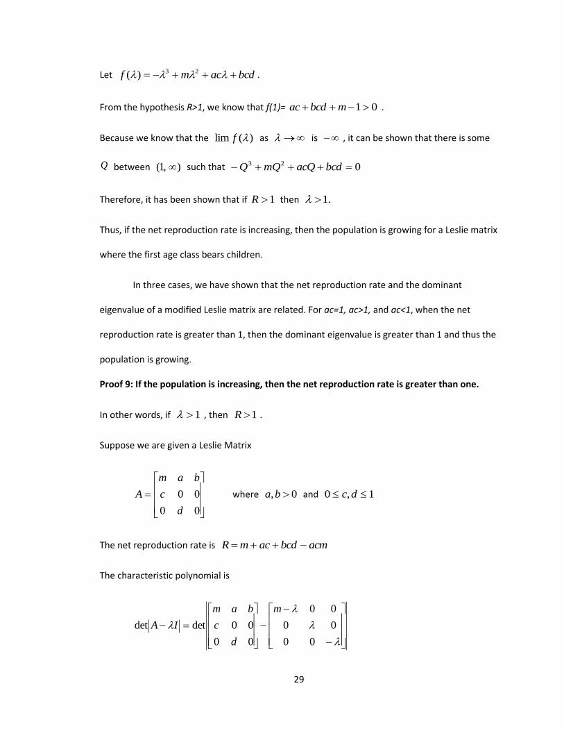
Proof 9: If the population is increasing, then the net reproduction rate is greater than one.
In other words, if 1 , then 1R .
Suppose we are given a Leslie Matrix
00
00
d
c
bam
A where 0, ba and 1,0 dc
The net reproduction rate is acmbcdacmR
The characteristic polynomial is
00
00
00
00
00detdet
m
d
c
bam
IA
30
d
c
bam
0
0det
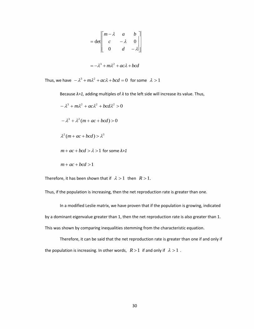
bcdacm 23
Thus, we have 023 bcdacm for some 1
Because λ>1, adding multiples of λ to the left side will increase its value. Thus,
02223 bcdacm
0)(23 bcdacm
32 )( bcdacm
1 bcdacm for some λ>1
1 bcdacm
Therefore, it has been shown that if 1 then .1R
Thus, if the population is increasing, then the net reproduction rate is greater than one.
In a modified Leslie matrix, we have proven that if the population is growing, indicated
by a dominant eigenvalue greater than 1, then the net reproduction rate is also greater than 1.
This was shown by comparing inequalities stemming from the characteristic equation.
Therefore, it can be said that the net reproduction rate is greater than one if and only if
the population is increasing. In other words, 1R if and only if 1 .
31
DISCUSSION
Leslie matrices have a wide variety of practical applications in and of themselves. Using
the Leslie matrix, as discussed above with projection and eigenvalues, it is possible for ecologists
and animal behaviorists to predict how a set number of individuals in a species will grow or
decline in total. With our research, we have found several shortcuts in this prediction process.
We take known facts from previous rules about Leslie matrices and streamline them to make
the process of predicting future growth or decline easier.
Through our research, we have successfully found associations between elements of a
Leslie matrix and the future growth or decline of the corresponding population. For instance, we
have discovered that knowing the survival probability of the first class and the reproductive
behavior of the second class is enough to determine whether the population will grow. As long
as these values, when multiplied together, are greater than or equal to 1, then the population
will grow. Also, we have found connections between the net reproduction rate and the
characteristic polynomial. The population is growing if and only if the net reproduction rate is
greater than 1. With this information, it is not necessary to solve for the eigenvalues of a Leslie
matrix in order to determine the future prospects of a population’s survival.
Not only have we looked at the general 3x3 case of the Leslie matrix, but we also
modified this case for incomplete data. By inserting variables into the first or last entry of the
Leslie matrix, we simulated the case where there is either no information on the beginning
stage(s) of a population or no information on the end stage(s) of a population, respectively.
Through this, we have discovered that there are relations amongst the elements and the
dominant eigenvalue of the matrix that can help predict the future growth or decline with more
ease.
32
Conclusion
The relationships between the various elements within Leslie matrices are extremely
interesting and make it much easier to determine information about a population. While there
has been research in this area, the results have been general and do not give many options as to
which elements are observed. With this paper, we hope to encourage more research into the
area of determining relationships between elements of the Leslie matrix and future growth of a
population. While the current research is an extension of previous work, there is much more to
discover with future research.
Direction of Further Research
While we have had positive results in looking for connections between future growth of
a population and elements of said population’s Leslie matrix, there are many possibilities for
research that have not been considered yet. For example, in the Leslie matrix, it would be
possible to work with more incomplete data so that there would be values for the entry in the
first row and first column along with values for the entry in the last row and last column. This
would give a different characteristic polynomial and net reproduction rate and further research
could tell whether the relationships we have discussed transfer over to this new case as well.
There are also other variations of the Leslie matrix to consider, such as the migration model.
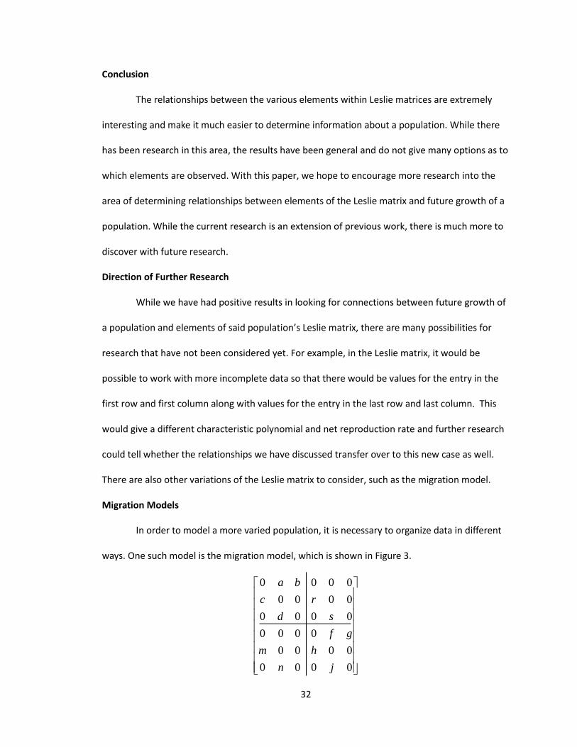
Migration Models
In order to model a more varied population, it is necessary to organize data in different
ways. One such model is the migration model, which is shown in Figure 3.
0000
0000
0000
0000
0000
0000
jn
hm
gf
sd
rc
ba
33
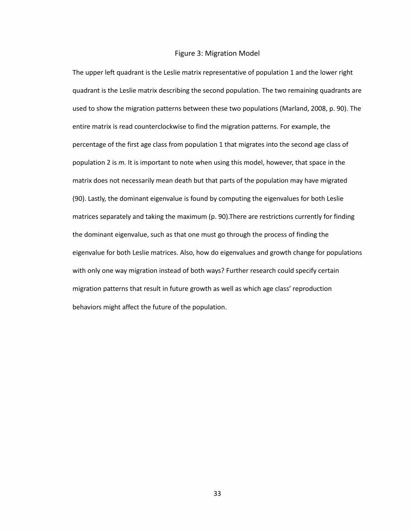
Figure 3: Migration Model
The upper left quadrant is the Leslie matrix representative of population 1 and the lower right
quadrant is the Leslie matrix describing the second population. The two remaining quadrants are
used to show the migration patterns between these two populations (Marland, 2008, p. 90). The
entire matrix is read counterclockwise to find the migration patterns. For example, the
percentage of the first age class from population 1 that migrates into the second age class of
population 2 is m. It is important to note when using this model, however, that space in the
matrix does not necessarily mean death but that parts of the population may have migrated
(90). Lastly, the dominant eigenvalue is found by computing the eigenvalues for both Leslie
matrices separately and taking the maximum (p. 90).There are restrictions currently for finding
the dominant eigenvalue, such as that one must go through the process of finding the
eigenvalue for both Leslie matrices. Also, how do eigenvalues and growth change for populations
with only one way migration instead of both ways? Further research could specify certain
migration patterns that result in future growth as well as which age class’ reproduction
behaviors might affect the future of the population.
WORKS CITED
34
Allen, L.J.S. (2007). An introduction to mathematical biology. Upper Saddle River, NJ:
Pearson Prentice Hall.
Anton, H., & Rorres, C. (1994). Elementary linear algebra: Applications version (7th
ed.). New York, NY: John Wiley and Sons, Inc.
Bacaër, N. (2011). A short history of mathematical population dynamics. New York, NY:
Springer Publishing.
Burks, R., Lindquist, J., & McMurran, S. (2008). What's my math course got to do with
biology? Primus: Problems, Resources, and Issues in Mathematics
Undergraduate Studies, 18(1), 71-84.
Caswell, H. (2001). Matrix population models: Construction, analysis, and interpretation
(2nd
ed.). Sunderland, MA: Sinauer Associates, Inc.
Keyfitz, N., & Caswell, H. (2005). Applied mathematical demography (3rd
ed.). New
York, NY: Springer Source + Business Media, Inc.
Lay, D.C. (2006). Linear algebra and its applications (3rd
ed.). New York, NY: Pearson
Addison Wesley.
Leslie, P.H. (1945). On the use of matrices in certain population mathematics.
Biometrika, 33(3), 183-212.
Marland, E., Palmer, K.M., & Salinas, R.A. (2008). Biological applications in the
mathematics curriculum. Primus: Problems, Resources, and Issues in
Mathematics Undergraduate Studies, 18 (1), 85-100.