LES of mixing in a jet mixer and combustion in a premixed swirling

free jet

OpenFOAM applications at the University of Rostock

Hannes Kröger

http://www.ltt-rostock.de/http://www.argo-group.de/

Outline● Introduction● Mixing Project

– SGS model implementations– Validation– Jet mixer simulations– Future work: inflow generator

● CIVB Project– Scope– Preliminary computations

Introduction: Institute for Technical Thermodynamics

LeadershipProf. Egon Hassel

Research groups● Numerical Thermodynamics● Experimental Thermodynamics● Thermodynamics of Engines

Employees● 15 scientists ● 3 OpenFOAM users

Outline● Introduction● Mixing Project

– SGS model implementations– Validation– Jet mixer simulations– Future work: inflow generator

● CIVB Project– Scope– Preliminary computations

SGS-Model implementation

Motivation● Change from Inhouse Fortran Code for LES to

OpenFOAM in progress● Best results in past simulations with DMM model● Some disadvantages in OpenFOAM:

– dynamic constant is averaged over entire domain and uniform everywhere

– Dynamic procedure in “dynamicMixedSmagorinsky” does not take Leonard stresses into account

“dynSmagorinsky” and “dynMixedSmagorinsky” were modified

Changes in “dynSmagorinsky”ij−

13kkij=−2C s2∣S∣ S ij

M ij= 2∣S∣ S ij−2∣S∣ S ijLij=ui u j− ui u j

C=C s2=−1

2 ⟨ LijM ij

⟨M klM kl ⟩ ⟩Present OpenFOAM implementation:

modified:

C=C s2=−1

2LijM ij

M klM kl

Constant is uniform – non-local in space

Constant varies in space

To ensure stability: clipping of backscatter 0C s21

Smagorinsky model:

Germano procedure:

⟨ .⟩ - denotes average)(

Reimplementation of DMM

ij−13kkij=ij

a= ui u j−ui u jLijm

a−2C s2∣S∣ S ij

mixed model:

Germano procedure (different from previous):

M ij= 2∣S∣ S ij−2∣S∣ S ijLij=ui u j− ui u j

H ij=ui u j−

uiu j−ui u j−ui u j

C=C s2=−1

2Lij M ij−H ijM klM kl

● Explicit grid filter implemented

● To ensure stability: clipping of constant and Leonard stresses

0C s21

Clipping procedure for Leonard stress

Asymptotical estimations Simple clipping procedure

● Stress terms from multiple filtered quantities may get very large, depending on grid resolution

Risk of instability

● Clark approximation is used to determine upper limit for filtered quantities:

Appeared in Communications In Numerical Methods In Engineering 2006, 22:55-61

Validation – Channel flow

x

y

Cyclic boundary

U

z

y

H=2

L=4Cyclic boundary

B=2

Resolution (nX x n

Y x n

Z): 128 x 40 x 64

Re=180

U=15.66

Solver: channelOodles

Channel Flow – ResultsMean Velocity Profile

Y (wall normal distance)

<U>

(Mea

n ax

ial v

eloc

ity)

Channel Flow – Reynolds Stress

R xx

R yy

y

Dynamic Mixed ModelDynamic Smagorinsky

R zz

Rey

nold

s st

ress

es

DMM Validation – Pitz & Daily case

x/H

U=13.3m/s Backward facing step:

● Geometry and mesh from “Xoodles” tutorial case● Solver: oodles

Streamwise velocity profiles at different positions:

H=0.025m

Outline● Introduction● Mixing Project

– SGS model implementations– Validation– Jet mixer simulations– Future work: inflow generator

● CIVB Project– Scope– Preliminary computations

Jet mixer – object of investigation

Ubulk

Ucoflow

L

Dd

●arrangement consists of pipe (diameter D) with coaxial nozzle (diameter d)

●fully developed turbulent flow in pipe (velocity Ucoflow

)●nozzle injects fluid with velocity U

bulk into pipe flow

●computational domain starts immediately behind nozzle (length L)

computationaldomain

Motivation●Investigation of micro-mixing in liquids●Jet mixer is of interest in chemical industry, applications are

● Homogenization● Chemical reactor

Jet mixer – flow modes

Jet like mode (A) Recirculation mode (B)

1V̇ D

V̇ dDd 1

V̇ D

V̇ dDd

Depending on volume flux ratio, two flow modes can be distinguished:

Time averaged mixture fraction fields

Jet mixer - investigations

Numerical● RANS (CFX 5)● LES (inhouse code)

– Dyn. Smagorinsky– DMM– Vortex Based Model

● LES (OpenFOAM)

Experimental● LIF (mixing)● LDA (velocities)

some limitations so far:● mixing only between fluids of equal density● no chemical reactions

LES of jet mixer - ResultsParameters of simulation●Pipe and nozzle diameter, velocities like in experimental setup●Resolution 700000 cells●Flow in Recirculation Mode (B)●Mixing water/water

r /D r /D

Axi

al V

eloc

ity U

Mix

ture

Fra

ctio

n f

Radial distribution at x/D=1.0

#

Jet mixer - Results

Mix

ture

Fra

ctio

n f

r /D r /D

Axi

al V

eloc

ity U

Radial distribution at x/D=1.5

Level of statistical modelling 1-point and time statistics

(Reynolds stress, kinetic energy)

1-point space and time statistics+

integral time and spatial length

1-point space and time statistics +

2-point space and time autocorrelations

Digital filter based method by (Klein et al. (2001))Spectral method (Lee et al (1992))Method of turbulent spots (Kornev et al. (2003))

2D random vortex method(Benhamadouche et al. (2003))Simple Random Generator (Lund et. al.(1998))……

Modified method of Kraichnan(Smirnov et al (2001), Batten et al.(2004))Diffusion approach (Kempf et al. (2005))2D random vortex method (FLUENT)……..

1

2

3

Inflow generation for LES/DNSIssue● Unsteady velocity boundary conditions must be prescribed at inlets● Common practice: adding white noise to mean profile or running

precursor simulationsBasic idea● Generation of artifical turbulence with prescribed statistical properties

Outline● Introduction● Mixing Project

– SGS model implementations– Validation– Jet mixer simulations– Future work: inflow generator

● CIVB Project– Scope– Preliminary computations

Vortex BreakdownCharacteristics●suddenly expansion of a rotating flow at some axial position●recirculation zone downstream

schematic

photograph

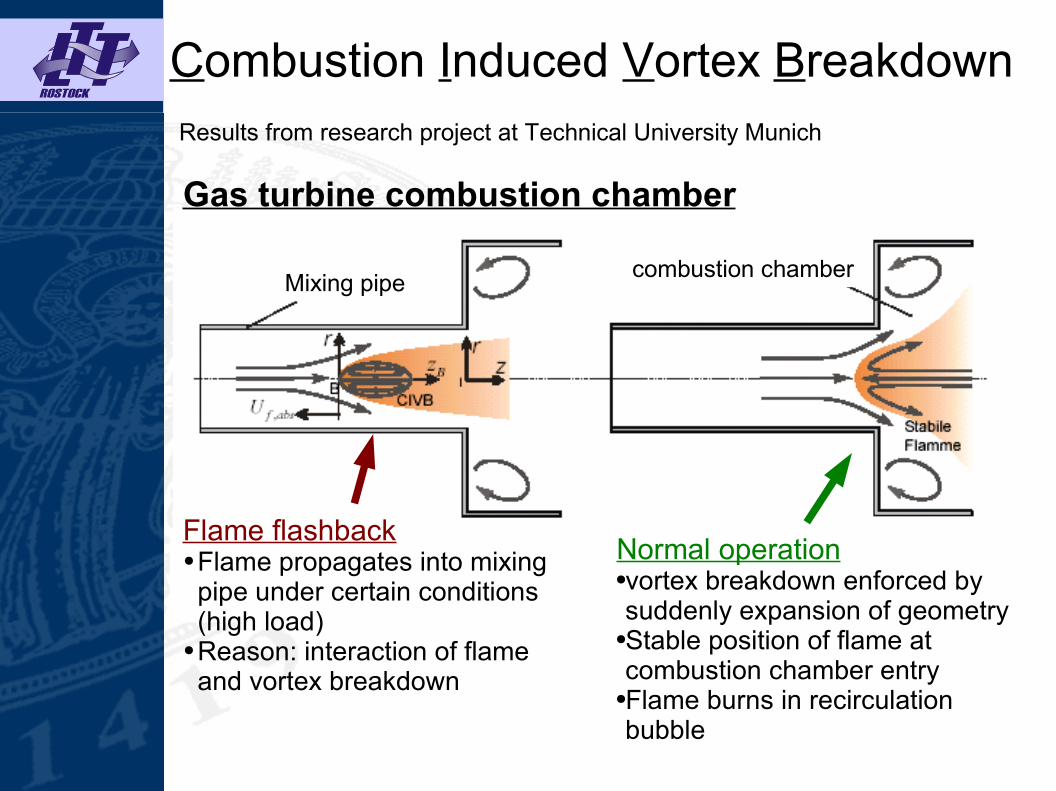
Combustion Induced Vortex Breakdown

Normal operation●vortex breakdown enforced by suddenly expansion of geometry

●Stable position of flame at combustion chamber entry

●Flame burns in recirculation bubble

Mixing pipe combustion chamber

Flame flashback● Flame propagates into mixing pipe under certain conditions (high load)

● Reason: interaction of flame and vortex breakdown

Gas turbine combustion chamber

Results from research project at Technical University Munich

CIVB in free vortices - experimental setup

Research at University of Rostock: CIVB in a free rotating jet● aim: understanding mechanisms of

upstream flame propagation in vortices● Experimental studies:

● OH-PLIF: tracking flame front● PIV: velocity field

● Numerical studies (OpenFOAM)

burner

swirl generator

nozzle

Simulation of experimental setup – model

wall

U=0.1m/sSlip wall

nozzle

∂ U∂ n

=0

p=1 bar

15cm

L=0.4m

D=0

.5m

d=5c

m

Resolution: 750 000 cells

● Up to now only qualitative studies (no measurements)● Simplified setup (no burner, bluff body for holding flame)

methaneair

flame

Nozzle boundary conditions

Nozzle withconical inset

Nozzle withcylindrical inset

rr

r

1m/s 1m/s

2m/s2m/s2m/s

UV

Vel

ocity

pro

files

in n

ozzl

e ex

it

r=5mm

More concentrated vortex:delta wing trailing vortex

● Simulations differ only in velocity profile in nozzle exit area

Simulation sequence

RANS solver: stationary cold flow

LES of cold flow(with fuel transport)

Ignition

LES of combustion

Conical nozzle: flame developmentt=t

0+85ms t=t

0+215ms

Flame stabilizes in front of flame holder

Cylinder nozzle: flame development

t=tign

+20ms t=tign

+50ms t=tign

+80ms

Acceleration of flame against main flow direction

Cylinder nozzle: flame tipt=t

ign+50ms

Isosurface T=2000K

Trailing vortex: flame development

t=tign

+5ms t=tign

+35ms t=tign

+85ms

Acceleration of flame against main flow direction

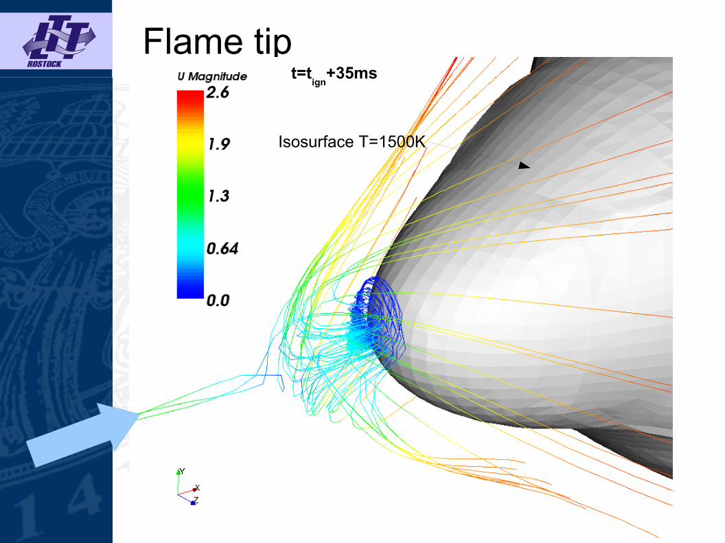
Flame tip

Isosurface T=1500K

t=tign

+35ms

Conclusion● Reimplementation of DMM model for

incompressible flows● Successful validation with turbulent

channel flow, backward facing step and coaxial jet mixer

● Identification of Combustion Induced Vortex Breakdown in LES with premixed combustion

Future works on OpenFOAM

● DMM model for variable density flows (modification of explicit filtering)

● DMM model for scalar transport (extension of “LESmodel”-class necessary)

● Generator for turbulent inflow conditions with prescribed statistical properties

● Presumed PDF/ILDM method for combustion and detailed chemistry modelling

Acknowledgement

We gratefully acknowledge the support of the ● OpenFOAM developer community● DFG (Deutsche Forschungsgemeinschaft)