Leonel Zuaznabar Moliner

A VERSION WITH CROSSING OF THE RANDOMDIRECTED FOREST AND ITS CONVERGENCE TO THE

BROWNIAN WEB

A thesis presented to the FederalUniversity of Rio de Janeiro infulfillment of the thesis requirementfor the degree of Doctor in Statistic.

Advisor: Glauco Valle

Rio de Janeiro - Brazil2017

ii

Leonel Zuaznabar Moliner

A VERSION WITH CROSSING OF THE RANDOMDIRECTED FOREST AND ITS CONVERGENCE TO THE

BROWNIAN WEB

Rio de Janeiro, of 2017.

Prof. Glauco Valle, Ph.D., UFRJ - Brazil.

Prof. Luiz Renato Fontes, Ph.D., USP - Brazil.

Prof. Maria Eulalia Vares., Ph.D., UFRJ - Brazil.

Prof. Leandro Pimentel , Ph.D., UFRJ - Brazil.

iii

Leonel Zuaznabar Moliner

A VERSION WITH CROSSING OF THE RANDOMDIRECTED FOREST AND ITS CONVERGENCE TO THE

BROWNIAN WEB

Prof. Cristian Favio Coletti, Ph.D., UFABC - Brazil.

iv

To my parents, Taty and Luis.

v

Acknowledgements

I would like to thank to: my advisor Glauco Valle, and the professors Maria EulaliaVares and Lenadro Pimentel, by all the math they taught me in the last four years;professor Luiz Renato Fontes, by help me in this project with very useful coments andsuggestion; family and friends for the support and the love given to me.

vi

Abstract

The Brownian web is the collection of graphs of coalescing one-dimensional Brownianmotions, starting from all possible starting points in one plus one-dimensional space/time.Several authors have studied convergence in distribution to the Brownian web, underdiffusive scaling of Markovian random walks. In a paper by R. Roy, K. Saha and A.Sarkar, convergence to the Brownian web is proved for a system of coalescing randompaths which are not Markovian: the Random Directed Forest (RDF). In view of the factthat paths in the RDF do not cross each other before coalescence, we study here a versionwhere crossing could happen and prove convergence to the Brownian web. This show howbroad is the class of coalescing paths that converges to the Brownian web; and providesan example of how the techniques to prove convergence to the Brownian web for systemsallowing crossings, can be applied to non-Markovian systems.

vii

TABLE OF CONTENTS

1 Introduction 11.1 The Brownian web . . . . . . . . . . . . . . . . . . . . . . . . . . . . . . 21.2 A version of the Random Directed Forest and the main result . . 3

2 Well posedness, renewal times and coalescing time 72.1 Well posedness . . . . . . . . . . . . . . . . . . . . . . . . . . . . . . . . 72.2 Renewal times . . . . . . . . . . . . . . . . . . . . . . . . . . . . . . . . 102.3 Coalescing time . . . . . . . . . . . . . . . . . . . . . . . . . . . . . . . . 14

3 Proof of the main result 253.1 Condition I . . . . . . . . . . . . . . . . . . . . . . . . . . . . . . . . . . 253.2 Condition B . . . . . . . . . . . . . . . . . . . . . . . . . . . . . . . . . . 333.3 Condition E . . . . . . . . . . . . . . . . . . . . . . . . . . . . . . . . . . 373.4 Condition T . . . . . . . . . . . . . . . . . . . . . . . . . . . . . . . . . . 42

Bibliography 49

viii

CHAPTER

ONE

INTRODUCTION

The study of the Brownian web started in 1979 with Arratia’s doutoral thesis ([1]). Heconstructed a process of coalescing one-dimensional Brownian motions starting from everypoint in R at time zero. Later Arratia, motivated by asymptotic of one-dimensionalvoter models, try to generalize this construction in [2] - an unpublished manuscript -to a process of coalescing Brownian motions, starting from every point in space andtime R × R. The Brownian web was not studied again until Toth and Werner in [15]- motivated by the construction of the continuum self-repelling motion - constructed aversion of the Brownian web. Years later Fontes, Isopi, Newman and Ravishankar gave adifferent construction in [8], [10], and used the first time the term Brownian web. Also inthese works the authors proved a criterium of convergence in distribution to this objectand used it to obtain the scaling limit of a system of coalescing random walks.

After [8] and [10] several authors have studied convergence in distribution to the Brow-nian web for different processes, for instance [4], [6], [7], [10], [11], [13] to mention someworks. The aim most of these papers is the understanding of the universality class associ-ated to the Brownian web. This was a breakthrough because it was an important questionin probability theory about how to characterize properly the convergence of systems ofcoalescing random walks which started to be studied by Arratia. From [8] and [10] thequestion about the universality class for the Brownian web arises as important one, sincemany important systems of coalescing random paths related to applications of probabilitytheory are more complicated; for instance they may have long range dependence, they arenot necessarily independent before coalescence and they are not necessarily Markovian.See for instance the Poisson Tree in [7], the Drainage Network Model studied in [5] and[6], the Random Directed Forest studied in [13] or the Direct Spaning Forest in [3], wherethe authors made a conjecture about the convergence to a transformation of the Brownianweb in its Remark 4.9 that was proved for a similar system in [11].

The main result of this thesis is Theorem 1.2.1. Something that we do not have inprevious works and show that the class of coalescing paths that converges to the Brownianweb is very wide.

In the remaining sections of this chapter we will present, at first, the space whereFontes, Isopi, Newman and Ravishankar defined the Brownian web. In the same Section1.1 we enunciate the theorem that characterizes the Brownian web proved in [10] and aconvergence criterium. In Section 1.2 we will introduce the Random Direct Forest studiedby Roy, Saha and Sarkar in [13], and define a version where paths could cross each other.At the end of this section we enunciate the main result of the thesis.

1

1.1 The Brownian web

In this section we will recall the space used in [8] and [10] to define the Brownian weband we will present the theorem proved there to characterize it. Also we will enunciate avariation of the convergence criterium proved in these papers.

Roughly speaking - as Fontes, Isopi, Newman and Ravishankar said in [10] - theBrownian web is the collection of graphs of coalescing one-dimensional Brownian motionsstarting from all possible starting points in one plus one-dimensional space/time. Eventhough it is difficult to think in coalescing Brownian motions starting at any space/timepoint of R2, fortunately - as the following Theorem 1.1.1 says - the Brownian web isfully determined by a countable number of coalescing Brownian motions starting from acountable dense subset D of R2.

In [10] the authors considered (R2, ρ), a completion of R2 under the metric ρ definedas

ρ((x1, t1), (x2, t2)

):=∣∣∣tanh(x1)

1 + |t1|− tanh(x2)

1 + |t2|

∣∣∣ ∨ ∣∣ tanh(t1)− tanh(t2)∣∣.

We may think R2 as the image of [−∞,∞]× [−∞,∞] under the mapping

(x, t)→(Φ(x, t),Ψ(t)

):=(tanh(x)

1 + |t|, tanh(t)

). (1.1.1)

For t0 ∈ [−∞,∞], let C[t0] be the set of functions from [t0,∞] to [−∞,∞] such thatΦ(f(t), t

)is continuous. Then define

Π =⋃

t0∈[−∞,∞]

C[t0]× {t0}.

For (f, t0) in Π, let us denote f the function that extends f to all [−∞,∞] by setting itequal to f(t0) for t ≤0. Take

d((f1, t1), (f2, t2)

)=(

supt≥t1∧t2

|Φ(f1(t), t)− Φ(f2(t), t)|)∨ |Ψ(t1)−Ψ(t2)|.

Let now H denote the set of compact subset of (Π, d) with the Hausdorff metric dH,

dH(K1, K2) := supg1∈K1

infg2∈K2

d(g1, g2) ∨ supg2∈K2

infg1∈K1

d(g1, g2),

for K1, K2 non-empty sets in H. FH is the Borel σ-field induced by (H, dH).The existence of a (H,FH)- valued random variable, called by Fontes, Isopi, Newman

and Ravishankar as the Brownian web, was proved in the Theorem 2.1 in [10]. We willpresent it in the following theorem.

Theorem 1.1.1. There exists a (H,FH)− valued random variable W whose distributionis uniquely determined by the following three properties:

(i) For any deterministic point (x, t) in R2 there exists almost surely an unique pathWx,t starting from (x, t).

(ii) For any deterministic n, (x1, t1), . . . , (xn, tn) the joint distribution of W(x1,t1), . . . ,W(xn,tn) is that of coalescing Brownian motions.

2

(iii) For any deterministic, dense countable subset D of R2, almost surely, W is theclosure in (H,FH) of {Wx,t : (x, t) ∈ D}.

The next Theorem 1.1.2 is a criterium of convergence to the Brownian web. Thistheorem is a variation of the Theorem 2.2 proved in [10] which can be found as theTheorem 1.4 in [12]. These theorems (Theorem 2.2 in [10] and Theorem 1.4 in [12]) havebeen the principal tools to prove the convergence to the Brownian web for many differentkind of coalescing system.

Theorem 1.1.2. Let {Yn}n≥1 be a sequence of (H,FH)-valued r.v. We have that {Yn}n≥1

converges to the Brownian web if the following conditions are satisfied:

(I) There exist some deterministic countable dense subset of R2, let us called D, andθyn ∈ Yn for any y ∈ D satisfying: for any deterministic y1, . . . , ym ∈ D, θy1n , . . . , θymnconverge in distribution as n → ∞ to coalescing Brownian motions starting iny1, . . . , ym.

(B) ∀β > 0, lim supn supt>β supt0,a∈R P[|ηYn(t0, t, a−ε, a+ε)| > 1

]→ 0 as ε→ 0+, where

ηYn(t0, t, a, b) ={y ∈ R× {t0 + t} : are touched by paths in Yn which also touch

some point in [a, b]× {t0}}.

(E) For some (H,FH)-valued r.v. Y and t > 0 take Y t− as the subset of paths in Y

which start before or at time t. If Zt0 is the subsequential limit of {Y t−0n }n≥1 for any

t0 in R, then for all t, a, b in R with t > 0 and a < b we get

E[|ηZt0 (t0, t, a, b)|

]≤ 1 +

b− a√πt.

(T ) Let ΛL,T := [−L,L]× [−T, T ] ⊂ R2 and for (x0, t0) ∈ R2 and ρ, t > 0,

R(x0, t0; ρ, t) := [x0 − ρ, x0 + ρ]× [t0, t0 + t].

For K ∈ H define AK(x0, t0; ρ, t) to be the event that K contains a path touchingboth R(x0, t0; ρ, t) and the right or the left boundary of the rectangle R(x0, t0; 20ρ, 4t).Then for every ρ, L, T ∈ (0,∞)

1

tlim supn→∞

sup(x0,t0)∈ΛL,T

P[AYn(x0, t0; ρ, t)

]→ 0 as t→ 0+.

1.2 A version of the Random Directed Forest and the

main result

R. Roy, K. Saha and A. Sarkar in [13] study the Random Directed Forest which is asystem of coalescing space and time random paths on Z2 as we now describe. Supposethat the first coordinate of a point in Z2 represents space and the second one time.We start a space/time random path in each point of Z2. The path starting at u in Z2

evolves as follows: every point in Z2 is open with some probability p or closed with 1− pindependently of each other. We say that a point v = (x, t) ∈ Z2 is above u = (x, t) if

3

t > t. If the path is at space/time position (v, t) then it jumps to the nearest open pointin the L1 norm above (v, t) if this nearest open point is unique. If it is not unique thenthe a choice is made uniformly to decide where the path has to jump to (see the Figure1.1). Note that two paths cannot cross each other and after one step it is possible toknow something about the future, that is to say, maybe we know if some points abovethe current position of the path are open or closed. That is why we get a system ofnon-Markovian random paths.

u

v

Figure 1.1: Open points in Z2 are marked by black dots. Note that the closest openpoints above u in the L1 distance are those connected by the dashed line. Hence the pathstarting at u moves to one of these points connected by the dashed line chosen uniformlyamong them; for instance it could be v.

In [13] the authors proved that under diffusive scaling, the closure of linearly interpola-tion trajectory induced by each discrete random path, in some space where the Brownianweb is defined, converges in distribution to the Brownian web. Our initial aim was toconsider a generalization of the random directed forest that allows crossings before coales-cence analogous to the generalized drainage models studied in [6]. This could be made ifwe do not impose the necessity that the jump should be made to the nearest open aboveposition. Although we get a well defined system, we were not able to prove convergenceto the Brownian web in this case. The problem here is to build a regeneration structuresimilar to that presented in [13], which is the way around the non-Markovianity of pathsin GRDF.

We will define a model which is slightly different from the Random Directed Forestand consider a generalization of it that allows crossing before coalescence. Suppose nowthat in each point u in Z2 we have a random variable Wu such that {Wu;u ∈ Z2} is ani.i.d. family of random variables in the set of positive integers. We will call the k-th levelof some u = (u(1), u(2)) in Z2 the following set

L(u, k) :={v = (v(1), v(2)) ∈ Z2 : v(2) > u(2) and ||v − u||1 = k

}, (1.2.1)

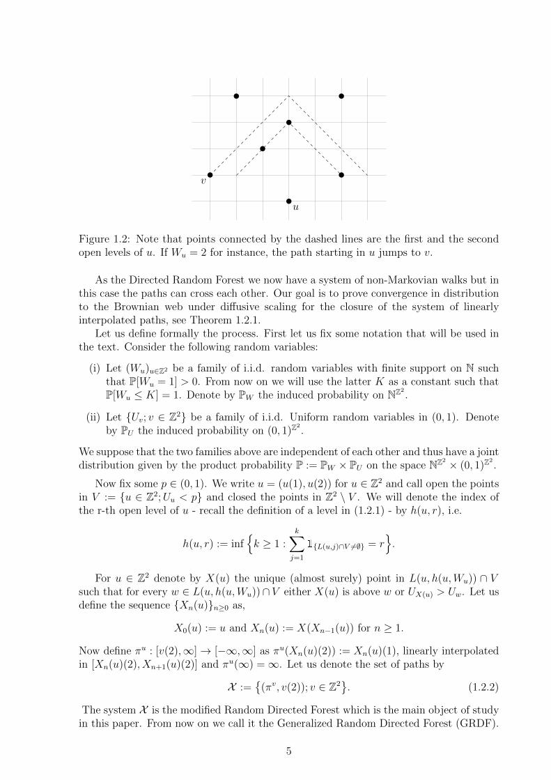
where for any u ∈ Z2, ||u||1 := |u(1)| + |u(2)|. A level L(u, k) is called open if it has atleast one open point. Now consider that the path not necessarily move to the nearestopen point above him, but to the the highest open point in the Wu-th open level. If thepath has two options to jump to, it makes an uniform choice to decide. See the Figure1.2 for an example.

4

u

v

Figure 1.2: Note that points connected by the dashed lines are the first and the secondopen levels of u. If Wu = 2 for instance, the path starting in u jumps to v.

As the Directed Random Forest we now have a system of non-Markovian walks but inthis case the paths can cross each other. Our goal is to prove convergence in distributionto the Brownian web under diffusive scaling for the closure of the system of linearlyinterpolated paths, see Theorem 1.2.1.

Let us define formally the process. First let us fix some notation that will be used inthe text. Consider the following random variables:

(i) Let (Wu)u∈Z2 be a family of i.i.d. random variables with finite support on N suchthat P[Wu = 1] > 0. From now on we will use the latter K as a constant such thatP[Wu ≤ K] = 1. Denote by PW the induced probability on NZ2

.

(ii) Let {Uv; v ∈ Z2} be a family of i.i.d. Uniform random variables in (0, 1). Denoteby PU the induced probability on (0, 1)Z

2.

We suppose that the two families above are independent of each other and thus have a jointdistribution given by the product probability P := PW × PU on the space NZ2 × (0, 1)Z

2.

Now fix some p ∈ (0, 1). We write u = (u(1), u(2)) for u ∈ Z2 and call open the pointsin V := {u ∈ Z2;Uu < p} and closed the points in Z2 \ V . We will denote the index ofthe r-th open level of u - recall the definition of a level in (1.2.1) - by h(u, r), i.e.

h(u, r) := inf{k ≥ 1 :

k∑j=1

1{L(u,j)∩V 6=∅} = r}.

For u ∈ Z2 denote by X(u) the unique (almost surely) point in L(u, h(u,Wu)) ∩ Vsuch that for every w ∈ L(u, h(u,Wu))∩ V either X(u) is above w or UX(u) > Uw. Let usdefine the sequence {Xn(u)}n≥0 as,

X0(u) := u and Xn(u) := X(Xn−1(u)) for n ≥ 1.

Now define πu : [v(2),∞]→ [−∞,∞] as πu(Xn(u)(2)) := Xn(u)(1), linearly interpolatedin [Xn(u)(2), Xn+1(u)(2)] and πu(∞) =∞. Let us denote the set of paths by

X :={

(πv, v(2)); v ∈ Z2}. (1.2.2)

The system X is the modified Random Directed Forest which is the main object of studyin this paper. From now on we call it the Generalized Random Directed Forest (GRDF).

5

We are interested in the diffusive rescaled GRDF. So let γ > 0 and σ > 0 be somefixed normalizing constants to be determined latter, u ∈ Z2 and n ∈ N. Let us define

πun(t) :=πu(n2γt)

nσfor t ∈ [0,∞), πun(∞) =∞

and

Xn :={

(πvn, v(2)) : v ∈ Z2}. (1.2.3)

The system of coalescing paths Xn is the rescaled GRDF and our aim is to prove thatits closure converges to the Brownian web as n goes to infinity.

Theorem 1.2.1. There exist positive constants γ and σ such that Xn, the closure of Xnin (H, dH), converges in distribution to the Brownian web as n goes to infinity.

6

CHAPTER

TWO

WELL POSEDNESS, RENEWAL TIMES AND

COALESCING TIME

In this chapter we first prove that Xn, the closure of Xn, is almost surely a compact set in(H, dH) for all n ≥ 1. Therefore we are indeed working with random elements of (H, dH)where the Brownian web is defined.

In Section 2.2 we prove the existence of regeneration times where the random pathsin the GRDF have no information about the future. The idea of using regeneration timescame from [13] and is fundamental since the paths seen at these times have the Markovproperty. However we are not able to get the existence as they did it, since in our casethe paths get into regions which have been observed before, something that the RandomDirected Forest model does not allow do and it is used in the proof given in [13]. So wewill follow a different approach here.

In Section 2.3 we will obtain an upper bound on the tail probability of the coalescencetime of two paths in X . This is a central estimate related to convergence to the Brownianweb. Related to other processes see [5],[6] and [13] for instance. The main ideas usedhere to get the bound come from these three works, although it is not a straightforwardapplication of the techniques used before. Here we have another important difference withthe Random Directed Forest studied in [13] because of the possibility of the paths to crosseach other before coalescence. This property does not allow us to follow the proof in [5]as done in [13]. We will need the ideas used in [6], where the authors work with a systemthat allows crossing, to control the coalescence time.

2.1 Well posedness

Lemma 2.1.1. Let N be some positive integer random variable and (ζn)n≥1 a non-negativesequence of identically distributed random variables. If for some k ≥ 1, δ > 0 and l >(k+2)(1+δ)

δwe have E[ζ

k(1+δ)1 ] and E[N l] finite, then for S :=

∑Nn=1 ζn we get that E[Sk] is

also finite.

Proof. We have that 0 ≤ S ≤ N max1≤j≤N ζj what implies that

Sk ≤ Nk max1≤j≤N

ζkj ≤ Nk

N∑j=1

ζkj .

7

Hence

E[Sk]≤ E

[Nk

N∑j=1

ζkj

]=∞∑n=1

nkn∑j=1

E[1{N=n}ζ

kj

].

Applying Holder inequality we get

E[Sk]≤

∞∑n=1

nkn∑j=1

E[ζk(1+δ)j

] 11+δP[N = n]

δ1+δ

= E[ζk(1+δ)1

] 11+δ

∞∑n=1

nk+1P[N = n]δ

1+δ .

Now applying Chebyshev inequality we get

E[Sk] ≤ E[ζk(1+δ)1

] 11+δ

∞∑n=1

nk+1E[N l]δ

1+δ

nlδ

1+δ

= E[ζk(1+δ)1

] 11+δE[N l]

δ1+δ

∞∑n=1

1

nlδ

1+δ−(k+1)

<∞.

For u ∈ Z2 define

CK(u) := {u(1), . . . , u(1) +K − 1} × {u(2)−K + 1, . . . , u(2)} .

We say that the box CK(u) is good if for all v ∈ CK(u), Wv = 1 and v is open.

Remark 2.1.1. We point out that when CK(u) is good then there are no paths crossingit and touching either (−∞, u(1)]× {u(2)} or [u(1) +K,∞)× {u(2)}.

Consider e1 = (1, 0) and define the following random variables

g+K(u) := inf{n ≥ 1 : CK(u+ (n− 1)Ke1) is good}

and

g−K(u) := inf{n ≥ 1 : CK(u− (nK − 1)e1) is good}.

Therefore CK(u+Kg+

K(u)e1

)is the first translation of CK(u) to the right of u by multiples

of K that is good and CK(u−Kg−K(e1)

)is the first translation of CK(u) to the left of u

by multiples of K that is good.

Our next result says that the number of paths in X starting before time t that crossa finite length interval at time t have finite absolute moment of any order.

Lemma 2.1.2. Let us define X t− as the set of paths in X that start before or at time tand by X t−(t) its values on time t. Then we have that

E[∣∣X t−(t) ∩ [a, b]

∣∣k] <∞for a < b ∈ R and k ≥ 1.

8

Proof. We will assume that t = a = 0 and b = 1. The general case is analogous. Forj ∈ Z let us define ζj := inf

{n ≥ 0 :

∑ni=0 1{(j,−i) is open } = K

}and the random region D

as

D :={v ∈ Z2 : −Kg−K((0, 0)) ≤ v(1) ≤ 1 +Kg+

K((0, 0)) and − ζv(1) ≤ v(2) ≤ 0}.

In next figure we show a possible face of D.

0 1

ζ0 = 7

ζ1 = 5

t = 0

Figure 2.1: In this picture we assume that K = 4. The blacks balls represent open pointsand the white ones represent closed points. The region D is given by the set of sites insidethe contour in bold. Note that g+

4 = 3 and g−4 = 2.

Recall that K is the support of W and note that, there are no paths of X crossing[0, 1]× {0} without landing in D, hence

∣∣X 0−(0) ∩ [0, 1]∣∣ ≤ ∣∣D∣∣ =

Kg+((1,0))∑j=1

ζj +

Kg−((0,0))∑j=0

ζ−j

Now using the Lemma 2.1.1 we have that E[∣∣X 0−(0) ∩ [0, 1]

∣∣k] <∞ for all k ≥ 1.

Proposition 2.1.1. We have that Xn, the closure in (H, dH) of Xn, is a compact set of(Π, d) for all n ≥ 1.

Proof. We will write the proof for X because for Xn is analogous. As in [12] we will showthat the mapping of X by (Φ(x, t),Ψ(t)) - recall the definition of (Φ,Ψ) in (1.1.1) - isequicontinuous. Note that by the properties of (Φ(x, t),Ψ(t)) it is enough to proof thecollection of that paths touching a box [−L,L]× [L,L] is equicontinuous, for any L > 0.Using Lemma 2.1.2 we have that the number of paths in X that cross [−L,L] × {k} isalmost surely finite, then the number of paths touching a box [−L,L] × [L,L] is almostsurely finite, and hence equicontinous.

The Lemma below allow us to consider the counting variables ηXn(t0, t, a, b) only oninteger starting times t0.

Lemma 2.1.3. Take a, b, t0, t ∈ R with a < b and t > 0, Xn as defined in (1.2.3), andηXn(t0, t, a, b) as in Theorem 1.1.2. Then for all ε > 0 there exists a constant Mε, notdepending on a, b, n, such that

P[|ηXn(t0, t, a, b)| > 1

]≤ P

[|ηX (0, n2γt, nσa−Mε, nσb+Mε)| > 1

]+ ε

for all t0 ∈ R, t > 0 and n ≥ 1.

9

Proof. Note that any path that cross [nσa, nσb]× {n2γt0} also cross the interval[nσa−Kg−K

((bnσac, bn2γt0c+ 1)

), nσb+Kg+

K

((bnσbc+ 1, bn2γt0c+ 1)

)]at time bn2γt0c+ 1. Then

P[|ηXn(t0, t, a, b)| > 1]

= P[|ηX (n2γt0, n

2γt, nσa, nγb)| > 1]

≤ P[∣∣ηX (bn2γt0c), n2γt, nσa−Kg−

((bnσac, bn2γt0c+ 1)

), nσb

+Kg+((bnσbc+ 1, bn2γt0c+ 1)

)∣∣ > 1].

Take Mε large enough such that

P[Kg−

((bnσac, bn2γt0c+ 1)

)> Mε] = P

[Kg+

((bnσbc+ 1, bn2γt0c+ 1)

)> Mε

]≤ ε

2.

Note that Mε does not depend on a, nor b, neither n.

By the translation invariant we get

P[|ηXn(t0, t, a, b)| > 1] ≤ P[|ηX (bn2γt0c, n2γt, nσa−Mε, nσb+Mε)| > 1

]+ ε

= P[|ηX (0, n2γt, nσa−Mε, nσb+Mε)| > 1

]+ ε.

2.2 Renewal times

As in [13] let us denote by ∆k(u), for k ∈ Z+ and u ∈ Z2, the set of points above Xk(u)whose configuration is already known; i.e. ∆0(u) = ∅ and for k ≥ 1,

∆k(u) :=[∆k−1(u) ∪

{v ∈ Z2 : ||v −Xk−1(u)||1 ≤ ||Xk(u)−Xk−1(u)||1

}]∩{v ∈ Z2 : v(2) > Xk(u)(2)

}. (2.2.1)

See Figure 2.2 as an example.

u

X1(u)

X2(u)

∆1(u)

Figure 2.2: Example for the dependence region ∆1(u). Note that in this example ∆2(u) =∅.

10

For any random variable τ(u) which satisfies ∆τ(u)(u) = ∅ we call Xτ(u)(u)(2) a renewaltime for the random path {Xk(u); k ≥ 1}. Note that τ(u) is not necessarily the first ksuch that ∆k(u) = ∅. The fact that the paths does not jump necessarily to first open levelabove it does not allow us to use the approach in [13] to verify existence and momentconditions of renewal times. The main result of this section is the following:

Proposition 2.2.1. Let u1, . . . , um be points in Z2 at the same time level, i.e with equalsecond component. Then there exist random variables T , Z and τ(ui) for i = 1, . . . ,msuch that T ≤ Z and

(i) ∆τ(ui)(ui) = ∅ and Xτ(u1)(u1)(2) = Xτ(ui)(ui)(2) for all i = 1, . . . ,m.

(ii) Taking T := Xτ(u1)(u1)(2) we have that its distribution depends on m but not onu1, . . . , um. For all k ≥ 1 we get E[T k] <∞. Note that πui(T ) = Xτ(ui)(ui)(1).

(iii) For all i = 1, . . . ,m we have sup0≤t≤T |πui(t) − ui(1)| ≤ Z and its distributiondepends on m but not on u1, . . . , um. Also for all k ≥ 1 we get E[Zk] <∞.

Proof. Without lost of generality we can assume that u1(2) = · · · = um(2) = 0. Foru ∈ Z2 let us define the following event E(u) as{

(u(1), u(2) + j) is open : j = 1, . . . , K}∩{W(u(1),u(2)+j) = 1 : j = 1, . . . , K − 1

}.

Note that on E(u) the path, that start in u and after some steps arrives in (u(1), u(2)+

K), knows nothing about the points above it. Now take {E1,1, E1,1, . . . , E1,m} independent

events such that P[E1,j] = P[E((0, 0))] for j = 1, . . . ,m and independent of the GRDFtoo. Let us define

D1 := {j ∈ {1, . . . ,m} : uj(1) = ui(1) for some 1 ≤ i < j}

andE1 := ∩

j∈{1,...,m}\D1

E(uj) ∩[∩

j∈D1

E1,j

].

On the event E1 the path that start at uj, after some τ(uj) steps, will arrive at (uj(1),uj(2) + K) and ∆τ(uj) = ∅, for j = 1, . . . ,m. We will find a sequence of independentevents {En}n≥1 with the same probability of success of E1 such that if En occurs for somen, we have a joint renewal time for the paths that start in u1, . . . , um. To do this let usmake some definitions. Define the following upper bound for the height of ∆1(u),

H(u) := inf{n ≥ 1 :

n∑j=1

1{(u(1),u(2)+j) is open } = K}. (2.2.2)

Let {H1,j; 1 ≤ j ≤ m} be a collection of i.i.d. random variables, independent of theGRDF model, and with the same distribution as H((0, 0)). Now define

ξ1 :=[

maxj∈{1,...,m}\D1

H(uj)]∨[

maxj∈D1

H1,j

].

11

u1 (Wu1 = 1) u2 (Wu2 = 2)

Xt1(u1)(u1) Xt1(u2)(u2)

ξ1 = 6

∆1(u1)

∆1(u2)

Figure 2.3: In the picture above we consider a realization of the random paths in theGRDF starting at u1 and u2. In this case ξ1 = 6 and one can see that the dependenceregion generated by the first for both paths are below u1(2) + ξ1. Moreover note thatXt1(u1)(u1) and Xt1(u2)(u2) are the last points visited by the paths starting respectively atu1 and u2 before time u1(2) + ξ1.

Now we will move each path until the first time that they need to observe over ξ1 todecide where to jump. These times could be defined as

t1(uj) := inf{n ≥ 1 : Xn(uj)(2) = ξ1 or

ξ1−Xn(uj)(2)∑i=1

1{L(uj ,i) is open } < WXn(uj)

},

for all 1 ≤ j ≤ m. Note that to define t1(uj) we do not need to see the points above ξ1.To help the understanding of the notation see Figure 2.3.

Now take {En,j; 1 ≤ j ≤ m,n ≥ 2} a family of independent event and independent of

the model too, such that P[En,j] = P[E((0, 0))] for all 1 ≤ j ≤ m and n ≥ 2. Also take

{Hn,j; 1 ≤ j ≤ m,n ≥ 2} an i.i.d. family of random variable independent of the modeland with the same distribution of H((0, 0)). Getting defined E1, . . . , Em and ξ1, . . . , ξnwe can define En+1 and ξn+1 as follows. First take tn(uj) as

inf{k ≥ 1 : Xk(uj)(2) = ξ1 + . . . ξn or WXk(uj) >

ξ1+...ξk−Xk(uj)(2)∑i=1

1{L(uj ,i) is open }

},

for all 1 ≤ j ≤ m. Define

Dn+1 :={j ∈ {1, . . . ,m} : Xtn(uj)(uj)(1) = Xtn(ui)(ui)(1) for some 1 ≤ i < j

}and

En+1 :=[

∩i∈{1,...,m}\Dn+1

E((Xtn(ui)(ui)(1), ξ1 + · · ·+ ξn)

)]∩[∩En,jj∈Dn+1

]ξn+1 :=

[max

j∈{1,...,m}\Dn+1

H((Xtn(uj)(uj)(1), ξ1 + · · ·+ ξn)

)]∨[

maxj∈Dn+1

Hn,j

].

12

Note that {ξn}n≥1 is an i.d.d. sequence and the distribution of ξn does not depend onu1(1), . . . , um(1). Also the probability of success of the event En does not depend onu1(1), . . . , um(1) and it is equal to P [E1]. Notice that if En happens fore some n thenwe get that

∑ni=1 ξi is a renewal time for the paths. Now defining the geometric random

variable M := inf{n ≥ 1 : 1En = 1} and τ(uj) = tM(uj) we get ∆τ(uj)(uj) = ∅ for all

1 ≤ j ≤ m. Defining T :=∑M

i=1 ξi we get that T = Xτ(uj)(uj)(2) for all 1 ≤ j ≤ mand applying Lemma 2.1.1, E[T l] <∞ for all l ∈ N. Note that the distribution of T doesnot depend on u1(1), . . . , um(1). Now see that for j = 1 . . . ,m by the construction of{ξk; k ≥ 1} and {tk(uj); k ≥ 1} we have

sup0≤t≤T

|πuj(t)− uj(1)| ≤M∑k=1

(ξ1 + · · ·+ ξk)2 ≤M(ξ1 + . . . ξM)2 ≤ (ξ1 + . . . ξM)3 := Z.

Using Lemma 2.1.1 we get E[Z l] <∞ for all l ≥ 1 and, by construction, the distribu-tion of Z does not depends on u1, . . . , um.

We can replicate recursively Proposition 2.2.1 to get:

Corollary 2.2.1. Let m ≥ 1 and u1, . . . , um be points in Z2 at the same level. Then thereexist sequences of random variables {Tj}j≥1, {Zj}j≥1 and {τj(ui)}j≥1 for i = 1, . . .m suchthat,

(i) ∆τj(ui)(ui) = ∅ and Xτj(u1)(u1)(2) = Xτj(ui)(ui)(2) for all i = 1, . . . ,m and j ≥ 1.Moreover for every i = 1, . . .m we have that τj(ui)−τj−1(ui), j ≥ 1, are i.i.d randomvariables.

(ii) Xτj(u1)(u1)(2) = Tj for j ≥ 1 and its distribution depends on m but not on u1 ,. . . ,um. For all k, j ≥ 1 we get that E[T kj ] < ∞ and for all j ≥ 1, i = 1 . . .m we havethat πui(Tj) = Xτj(ui)(ui)(1). Moreover Tj −Tj−1, j ≥ 1, are i.i.d random variables.

(iii) supTj−1≤t≤Tj |πui(t) − πui(Tj−1)| ≤ Zj for all i = 1, . . . ,m and j ≥ 1. The random

variables Zj, j ≥ 1, are i.i.d and their common distribution depends on m but noton u1, . . . , um. For all k, j ≥ 1 we get that E[Zk

j ] <∞.

Fix points u1, . . . , um in Z2. To simplify, suppose that u1 is at the same time level orabove ui for every i = 2, . . .m. Then we can obtain a similar renewal structure for pathsin X , that do not start necessarily at the same time level, moving each path πu2 , . . . , πum

up to the first time they need to see above u1(2) to move, and after that use the sameidea of Proposition 2.2.1.

Corollary 2.2.2. Let m ≥ 1 and u1, . . . , um be points in Z2 such that u1 is at the sametime level or above ui for every i = 2, . . .m. Then there exist sequences of random variables{Tj}j≥1, {Zj}j≥1 and {τj(ui)}j≥1 for i = 1, . . .m such that,

(i) ∆τj(u1)(u1) = ∆τj(ui)(ui) = ∅ and Xτj(u1)(u1)(2) = Xτj(ui)(ui)(2) for all i = 1, . . . ,mand j ≥ 1. Moreover we have that τj(u1) − τj−1(u1), j ≥ 1, are i.i.d randomvariables, and for every i = 2, . . .m we have τj(ui) − τj−1(ui), j ≥ 2, are i.i.drandom variables.

13

(ii) Xτj(ui)(ui)(2) = Tj for all i = 1, . . .m and j ≥ 1. Also for all j ≥ 1, i = 1 . . .m wehave that πui(Tj) = Xτj(ui)(ui)(1). The distribution of Tj depends on m but not onu1, . . . , um and for all k, j ≥ 1 we get that E[T kj ] <∞. Moreover Tj − Tj−1, j ≥ 2,are i.i.d random variables.

(iii) supTj−1≤t≤Tj |πu1(t)−πu1(Tj−1)| ≤ Zj for all j ≥ 1, and for every i = 2, . . .m we have

that supTj−1≤t≤Tj |πui(t) − πui(Tj−1)| ≤ Zj for all j ≥ 2. The random variables Zj,

j ≥ 1, are i.i.d and their common distribution depends on m but not on u1, . . . , um.For all k, j ≥ 1 we get that E[Zk

j ] <∞.

2.3 Coalescing time

The aim of this section is to prove the following Proposition 2.3.1, extremely useful toprove the conditions of Theorem 1.1.2.

Proposition 2.3.1. Let us define ν := inf{t ≥ 0 : π(0,0)(s) = π(0,1)(s) for all s ≥ t}.Then there exist a positive constant C > 0 such that

P[ν > k] ≤ C√k.

As an immediate consequence of Proposition 2.3.1 we have:

Corollary 2.3.1. Let u = (0, 0), v = (0, l) and

ν(u, v) := inf{t ≥ 0 : πu(s) = πv(s) for all s ≥ t}.

Then there exist positive constant C such that

P[ν(u, v) > k] ≤ Cl√k.

Proof. Since {ν(u, v) > k} ⊂ ∪li=1{ν((i− 1)e1, ie1

)> k} we have that

P[ν(u, v) > k] ≤l∑

i=1

P[ν((i− 1)e1, ie1

)> k]≤ Cl√

k. (2.3.1)

We will need some previous results to prove Proposition 2.3.1. First, we are goingto construct another sequence of renewals times (Ti)i≥1 for two paths. The ideas usedto get theses new times, are the same one used in Section 2.2.1, hence some details willbe omitted. We will see later why in this section we need to consider this new renewalstructure.

Let u and v two points in Z× {0}. Let (T ui )i≥1 be the renewals for the path πu thatwas getting in Corollary 2.2.1. Now move the path πv up to the first time that they needto see above T u1 −K, and see if the points between T u1 −K and T u1 , in the same y−axisof the point where you stopped the path πv, are open and with the respectively randomvariables W ’s, equals to one. If this happens, we have that in T u1 , the paths πu and πv

renews together. If not, we move the path πv, up to the first time to need to see above

14

T u2 −K t, and again, see the appropriated K points between [T u2 −K,T u2 ] and ask the samequestion. Repeat this procedure until we get a ”yes”. By construction, we know nothingabout the points between T uj − K and T uj , for any j ≥ 1 ,unless the ones associated tothe path πu. Then we get a common renewal time

T :=G∑i=1

T ui

where G is a geometric random variable. See that G does not depend on the displacementof πv, hence T does not depend. Also the law of T does not depend on v. Now define therandom variable

Z :=G∑i=1

(Ti)2.

Then we have that

|πu(T )− πv(T )| ≤ 2Z.

In view of G does not depend on the displacement of πu, for all m ∈ N, taking u = (0, 0)and v = (0,m), we have that

π(0,0)(T )− π(m,0)(T )|{π(0,0)(T )− π(m,0)(T ) < 0}st

≥ −2Z. (2.3.2)

Repeating this construction we get a sequence of common renewals times (Ti)i≥1 and

i.i.d. random variables (Zi)i≥1.

Let be u0 := (0, 0) and for m ∈ N take um := (m, 0) define

Y m0 := m and Y m

n := πumn (Tn)− πu0n (Tn) for n ≥ 1. (2.3.3)

The process Y m represents the distance between the paths π(0,0) and π(0,m) on the renewaltimes for the pair (π(0,0), π(0,m)).

By the Skorohood’s Representation Theorem, there exist a Brownian motion (B(s))s≥0

starting in m and stopping times (Si)i≥0 such that

B(Si)d= Yi, for i ≥ 0

and (Si)i≥0 has the following representation:

S0 := 0, Si := inf{s ≥ Si−1 : B(s)−B(Si−1) /∈

(Ui(B(Si−1)), Vi(B(Si−1))

)}where

{(Ui(m), Vi(m)) : m ∈ Z, i ≥ 1

}is a family of independent random vectors taking

values in((Z− − {0})× N

)∪{

(0, 0)}

.

Lemma 2.3.1. For any borel set A, let us define νmA

as the first hitting time to A of thesequence {Y m

n }n≥1; i.e.νmA

:= inf{n ≥ 1 : Y mn ∈ A}.

Then

15

(i) For all m ∈ N we have P[νm(−∞,0] <∞

]= 1.

(ii) supm<0 E[Y mvm[0,∞)

]<∞.

(iii) infm≥1 P[Y mνm(−∞,0]

= 0]> 0.

(iv) Let us define the sequence (al)l≥1 as

a1 := inf{n ≥ 1 : Y 1n ≤ 0} and for l ≥ 2,

and

al :=

{inf{n ≥ al−1 : Y 1

n ≥ 0}; if l is eveninf{n ≥ al−1 : Y 1

n ≤ 0}; if l is odd.

Then there exists a constant c1 < 1 such that

P[Y 1aj6= 0, for j = 1, . . . , k] ≤ ck1,

for all k ≥ 1.

Proof. Let us start proving item (i). Define

D :={n ∈ [1, νm(−∞,0]] ∩ N : (B(s))s≥0 visits (−∞, 0] in the interval (Sn−1, Sn]

}Since m > 0, for any n ∈ D, one of the following things should occur:

(a) Un(B(Sn−1))+B(Sn−1) = 0. This implies that n = νm(−∞,0], since B(Sn) = B(Sn−1)+

Un(B(Sn−1)).

(b) Un(B(Sn−1)) + B(Sn−1) < 0. In this case we have that (B(s))s≥0 visits zero in theinterval (Sn−1, Sn], before hitting {Vn(B(Sn−1))+B(Sn−1), Bn(B(Sn−1))+B(Sn−1)}.Since B(Sn) − B(Sn−1)

d= Yn − Yn−1, we get - using Strong Markov property and

(2.3.2) - that the probability of an Standard Brownian motion, independent of Z,

leaves the interval [−2Z, 1] by the left side, is a lower bound to the probability thatB(Sn) = U(B(Sn−1)) +B(Sn−1).

Hence #D ≤ G, where G is a Geometric random variable. Then #D < ∞ almostsurely. Let us see this implies νm(−∞,0] < ∞ almost surely. If νm(−∞,0] = ∞ and #D < ∞,

taking j = max{n ∈ D}, we have that (B(s))s≥0 does not visits zero after Sj; whathappens with probability zero.

Let us prove item (ii). By item (i) we have that for all m ∈ N

E[Y mvm[0,∞)

]≤ E

[ G∑i=1

2Zi]<∞.

To prove (iii) consider m,M ∈ N with m > M and define the stopping time

νm(−∞,M ] := inf{n ≥ 1 : Y mn ≤M}.

16

It is easy to see that νm(−∞,M ] ≤ νm(−∞,0], hence by the item (i) we get that νm(−∞,M ] is finitealmost surely. Also note that

P[Y mνm(−∞,0]

= 0] ≥ P[Y mνm(−∞,0]

= 0, νm(−∞,0] 6= νm(−∞,M ]]

=M∑k=1

P[Y mνm(−∞,0]

= 0, Y mνm(−∞,M ]

= k]

=M∑k=1

P[Y mνm(−∞,0]

= 0|Y mνm(−∞,M ]

= k]P[Y mνm(−∞,M ]

= k].

For all 1 ≤ k ≤ M by Strong Markov property of (Y mn )n≥0 and the translation invariant

of the model, we have that

P[Y mνm(−∞,0]

= 0|Y mνm(−∞,M ]

= k] = P[Y kνk(−∞,0]

= 0].

Hence

P[Y mνm(−∞,0]

= 0] ≥M∑k=1

P[Y kνk(−∞,0]

= 0]P[Y mνm(−∞,M ]

= k]

≥(

min1≤k≤M

P[Y kνk(−∞,0]

= 0]) M∑k=1

P[Y mνm(−∞,M ]

= k]

=(

min1≤k≤M

P[Y kνk(−∞,0]

= 0])P[νm(−∞,0] 6= νm(−∞,M ]]

≥(

min1≤k≤M

P[Y kνk(−∞,0]

= 0])(

infm>M

P[νm(−∞,0] 6= νm(−∞,M ]]).

From the description of the GRDF it is straightforward to verify that P[Y kνk(−∞,0]

= 0] > 0

for all k ≥ 1, and then, min1≤k≤M P[Y kνk(−∞,0]

= 0] > 0. Now let us to prove that for an

adequate M we haveinfm>M

P[νm(−∞,0] 6= νm(−∞,M ]] > 0.

Note that P[νm(−∞,0] = νm(−∞,M ]] = P[Y mνm(−∞,M ]

≤ 0]. By the symmetry and the invariant

translation property of the GRDF model, we have

P[Y mνm(−∞,M ]

≤ 0] = P[Y(M−m)

ν(M−m)[0,∞)

≥M ] ≤ 1

ME[Y

(M−m)

ν(M−m)[0,∞)

]≤ 1

Msupm<0

E[Y mvm[0,∞)

].

By item (ii) we have that supm<0 E[Y mvm[0,∞)

]<∞, hence taking M such that

c :=1

Msupm<0

E[Y mvm[0,∞)

]< 1,

we get

infm>M

P[Y mνm(−∞,0]

= 0] ≥(

min1≤k≤M

P[Y kνk(−∞,0]

= 0])

(1− c

M) > 0,

which completes the proof of (iii).

17

Now we prove (iv). Define

c1 := supm≥1

P[Y ma16= 0].

By the item (iii) we have c1 < 1. By definition P[Y 1a16= 0] ≤ c1. The proof will follow

by induction on k. Suppose that P[Y 1aj6= 0, for j = 1, . . . , k] ≤ ck1. Here we are going to

assume that k is even, the case k odd is similar. Write

P[Y 1aj6= 0 for j = 1, . . . , k + 1]

=∑m≥1

P[Y 1ak+16= 0, Y 1

ak= m,Y 1

aj6= 0 for j = 1, . . . , k − 1]

=∑m≥1

P[Y 1ak+16= 0|Y 1

ak= m,∩k−1

j=1{Y 1aj6= 0}]P[Y 1

ak= m,∩k−1

j=1{Y 1aj6= 0}].

By Strong Markov property of (Y 1n )n≥0 and the translation invariant of the GRDF model,

we have that

P[Y 1ak+16= 0|Y 1

ak= m,Y 1

aj6= 0 for j = 1, . . . , k − 1] = P[Y m

a16= 0] ≤ c1.

Hence

P[Y 1aj6= 0 for j = 1, . . . , k + 1] ≤ c1

∑m≥1

P[Y 1ak

= m,Y 1aj6= 0 for j = 1, . . . , k − 1]

= c1P[Y 1aj6= 0 for j = 1, . . . , k]

≤ ck+11 .

Lemma 2.3.2. Consider the sequence (al)l≥1 as in the previous lemma and (B(s))s≥0 and(Sn)n≥1 obtained from the Skorohood’s Representation of Y 1. Then there exist random

variables (Ri)i≥1 and R0 independent of (B(s))s≥0 such that

(i) Ri|{Ri 6= 0} d= R0 for all i ≥ 1.

(ii) Sal is stochastically dominated by Jl, which is defined as J0 = 0,

J1 := inf{s ≥ 0 : B(s)−B(0) = −(R1 + R0)},

and

Jl := inf{s ≥ Jl−1 : B(s)−B(Jl−1) = (−1)l(Rl +Rl−1)}, l ≥ 2.

(iii) Yal 6= 0 implies B(Jl) 6= 0.

18

Proof. The proof is similar to the proof of Lemma 3.5 in [6]. By Skorohood RepresentationTheorem we have a Brownian motion (B(s))s≥0 starting in 1 and stopping times (Sn)n≥0,which could be both taken independent of (Y 1

n )n≥1, such that

Y 1n − Y 1

n−1d= B(Sn)−B(Sn−1) , for all n ≥ 1.

There exists a sequence of random variables (Zn)n≥1 such that |Y 1n − Y 1

n−1| ≤ 2Zn . Then

|B(Sn)−B(Sn−1)|st

≤ 2Zn , for all n ≥ 1. (2.3.4)

Recall that (Si)i≥0 has the following representation.

S0 := 0, Si := inf{s ≥ Si−1 : B(s)−B(Si−1) /∈

(Ui(B(Si−1)), Vi(B(Si−1))

)}(2.3.5)

where{

(Ui(m), Vi(m));m ∈ Z, i ≥ 1}

is a family of independent random vectors takingvalues in

((Z− − {0})× N

)∪{

(0, 0)}

.By (2.3.4) and (2.3.5) we have that

−2Znst

≤ infSn−1≤s≤Sn

{B(s)−B(Sn−1)} ≤ supSn−1≤s≤Sn

{B(s)−B(Sn−1)}st

≤ 2Zn (2.3.6)

As in the proof of Lemma 2.3.1 consider the following random set

C :={n ∈ [1, τ(−∞,0]] ∩ N : (B(s))s≥0 visits (−∞, 0] in the interval (Sn−1, Sn]

}.

Note that

−|C|∑i=1

2Zist

≤ inf0≤s≤τ(−∞,0]

B(s) .

There exists a geometric random variable G (see the proof of item (i) of Lemma 2.3.1)such that G ≥ |C|. Then we have

−G∑i=1

2Zist

≤ inf0≤s≤τ(−∞,0]

B(s).

Let us define the random variable R1 as

R1 :=

{−∑G

i=1 2Zi; if |C| > 10; otherwise,

and R0 as an independent random variable such that R0d= R1|{R1 6= 0}. Define

J1 := inf{s ≥ 0 : B(s)−B(0) = −(R1 + R0)}

which is clearly stochastically above Sa1 . Let (B(s))s≥0 be (B(s))s≥0 translated to have

B(0) = R0, then Ya1 6= 0 is equivalent to B(J1) 6= 0, indeed

Ya1 6= 0⇔ R1 > 0⇔ B(J1) < 0 .

From this point, it is straightforward to use an induction argument to build the se-quence {Rj}j≥1. At step j in the induction argument, we consider initially an excursionof (B(s))s≥0 in a time interval of size (Saj −Saj−1

), and since |Y naj−1| ≤ Rj−1 we can obtain

Rj and define Jj using (B(s))s≥0 as before. By the strong Markov property of (Y 1n ), we

obtain that the Rj’s are independent and Yaj 6= 0 is equivalent to B(Jj) 6= 0.

19

Now consider Yn := Y 1n for all n ≥ 1 and take νY := inf{n ≥ 1 : Y 1

n = 0}. We willobtain the Proposition 2.3.1 from the following lemma:

Lemma 2.3.3. There exist positive constants C1 and C2 such that

P[νY > k] ≤ C1√k

(2.3.7)

and

P[TνY > k] ≤ C2√k

for all k ≥ 1. (2.3.8)

for every k ≥ 1.

Proof. Let us suppose that (2.3.7) is true and use it to prove (2.3.8) with the same ideaused in [13]. Recall from Corollary 2.2.1 that T1 has finite moments and define the constantL := 1/2E[T1] and take k ∈ N then

P[TνY > k] ≤ P[TνY > k, νY ≤ Lk] + P[νY > Lk] ≤ P[TbLkc > k] + P[νY > Lk].

By (2.3.7), it is enough to prove that P[TbLkc > k] ≤ C3√k

for some constant C3. Then

P[TbLkc > k

]= P

[ bLkc∑i=1

[Ti − Ti−1] > k]

= P[ bLkc∑i=1

[Ti − Ti−1]− bLkcE[T1] > k − bLkcE[T1]]

≤Var

[∑bLkci=1 (Ti − Ti−1)

](k − bLkcE[T1]

)2

=bLkcVar[T1](k − bLkcE[T1]

)2 .

Note that

√kbLkcVar[T1](k − bLkcE[T1]

)2 → 0 as k → 0.

Then there exist M such that

bLkcVar[T1](k − bLkcE[T1]

)2 ≤1√k

for all k ≥M. Then we can find a sufficiently large constant C3 > 0 such that

bLkcVar[T1](k − bLkcE[T1]

)2 ≤C3√k

20

for all k ≥ 1.

Now we prove (2.3.7). Here we simply write Y = Y 1. Recall the definition of (B(s))s≥0

and (Si)i≥0 above for the case m = 1. For δ > 0 to be fixed later and every k ∈ N wehave that,

P[νY > k] = P[Sk ≤ δk, νY > k] + P[Sk > δk, νY > k]. (2.3.9)

To get an upper bound for P[Sk ≤ δk, νY > k] we use the Skorohod representation:

Sk =k∑i=1

(Si − Si−1

)=

k∑i=1

Qi(Yi−1),

where{Qi(m); i ≥ 1,m ∈ Z

}are independent random variables and Qi(m) is independent

of (Y1, ..., Yi−1) for all i ∈ N,m ∈ Z. Note that on {νY > k} we have that Yi 6= 0 fori ∈ {1, . . . , k}. Now, for fixed λ > 0, we have

P[Sk ≤ δk, νY > k] = P[e−λSk ≥ e−λδk, νY > k] ≤ eλδkE[e−λSk1{νY >k}]

Claim 2.3.1.

E[e−λSk1{νY >k}] ≤(

supm∈Z\{0}

E[e−λQ(m)])k,

where, for each m, Q(m) is a random variable with the same distribution of Q1(m).

Proof of Claim 2.3.1. The proof is essentially the same given in Theorem 4 in [5] and weinclude it here for the sake of completeness. Taking Fk := σ(Y1, . . . , Yk) we have that

E[e−λSk1{νY >k}] = E[E[e−λSk1{νY >k}|Fk−1]

]≤ E

[e−λSk−1E[e−λQk(Yk−1)

1{νY >k−1}1{Yk−1 6=0}|Fk−1]]

= E[e−λSk−11{νY >k−1}E[e−λQk(Yk−1)

1{Yk−1 6=0}|Fk−1]]

and

E[e−λQk(Yk−1)1{Yk−1 6=0}|Fk−1] =

∑m∈Z\{0}

E[e−λQk(m)1{Yk−1=m}|Fk−1]

=∑

m∈Z\{0}

1{Yk−1=m}E[e−λQk(m)|Fk−1]

=∑

m∈Z\{0}

1{Yk−1=m}E[e−λQ(m)]

≤ supm∈Z\{0}

E[e−λQ(m)].

So, applying the above argument recursively we obtain

E[e−λSk1{νY >k}] ≤ E[e−λSk−11{νY >k−1}](

supm∈Z\{0}

E[e−λQ(m)])≤(

supm∈Z\{0}

E[e−λQ(m)])k.

21

Using Claim 2.3.1 we get that

P[Sk ≤ δk, νY > k] ≤(eλδ sup

m∈Z\{0}E[e−λQ(m)]

)k.

Let Q−1,1 be the exit time of interval (−1, 1) by a Standard Brownian motion. Wehave that

E[e−λQ(m)

]= E

[e−λQ(m)|(U(m), V (m)) 6= (0, 0))

]P[(U(m), V (m)) 6= (0, 0)]

+ P[(U(m), V (m)) = (0, 0)

]≤ E

[e−λQ−1,1

](1− P

[(U(m), V (m)) = (0, 0)

])+ P

[(U(m), V (m)) = (0, 0)

]= P

[(U(m), V (m)) = (0, 0)

](1− c2) + c2 , (2.3.10)

where c2 = E[e−λQ−1,1

]< 1.

Claim 2.3.2. 0 < c3 := supm∈Z\{0} P[(U(m), V (m)) = (0, 0)

]< 1.

Proof of Claim 2.3.2. The proof uses the hypothesis that P (W = 1) > 0. However by astraightforward adaptation, one can see that this is not required for the claim to remainvalid.

We follow the idea used in [13]. Notice that

P[(U(m), V (m)

)= (0, 0)] = P[Yn+1 = m|Yn = m].

Then (see Figure 2.4) we have

P[(U(m), V (m)

)= (0, 0)] ≥ (pP[W = 1])2.

u v

Figure 2.4: If Wu = Wv = 1 and u+e2 and v+e2 are open, which occurs with probability(pP[W = 1])2.

So c3 := supm∈Z\{0}

{P[(U(m), V (m)

)= (0, 0)]

}≥ (pP[W = 1])2 > 0.

For the upper bound in the statement, see that

P[(U(m), V (m)

)6= (0, 0)] = P[Yn+1 6= m|Yn = m].

Hence we have that (see Figure 2.5)

P[(U(m), V (m)

)6= (0, 0)] ≥ (1− p

2)p3(1− p)3(P[W = 1])3,

22

u v

Figure 2.5: If Wu = Wv = Wv+e1+e2 = 1 and u+ 2e2, v+ e1 + e2 and v+ e1 + 2e2 are openand u+ e2, v + e2 and v + 2e2 are closed, then with p3(1− p)4(P[W = 1])3 if |m| = 1 and(1 − p

2)p3(1 − p)3(P[W = 1])3 in case |m| 6= 1, we have the trajectory as represented in

the picture.

Hence infm∈Z\{0} P[(U(m), V (m)

)6= (0, 0)] ≥ (1− p

2)p3(1− p)3(P[W = 1])3. So,

c3 ≤ 1− (1− p

2)p3(1− p)3(P[W = 1])3 < 1.

Using Claim 2.3.2 and (2.3.10), we obtain that

E[e−λQ(m)

]≤ c3(1− c2) + c2 .

Now chose δ such that c4 := eδλ[c3(1− c2) + c2

]< 1. Then

P[Sk ≤ δk, νY > k] ≤ ck4 ≤c5√k, (2.3.11)

for some suitable c5 > 0. This gives the bound we need on the first term of (2.3.9). Letjust prove the previous claim before dealing with the second term in (2.3.9).

Now we consider the second term in (2.3.9). To deal with it we consider an approachsimilar to [6]. Take the sequence (al)l≥0 as in the statement of Lemma 2.3.1. Note that

P[νY > k, Sk > δk] ≤k∑l=1

P[νY > k, Sk ≥ δk, Sal−1< δk, Sal ≥ δk] . (2.3.12)

For now fix l = 1, . . . k, using Lemma 2.3.2 we get,

{νY > k, Sk ≥ δk, Sal−1< δk, Sal ≥ kδ} ⊆ {Yaj 6= 0, for j = 1, . . . , l − 1, Sal ≥ kδ},

hence

P[νY > k, Sk ≥ δk, Sal−1< δk, Sal ≥ kδ]

≤ P[Yaj 6= 0, for j = 1, . . . , l − 1, Sal ≥ kδ]

≤ P[Yaj 6= 0, for j = 1, . . . l − 1, Jl ≥ kδ]

= P[Jl ≥ kδ|Yaj 6= 0, for j = 1, . . . l − 1]P[Yaj 6= 0, for j = 1, . . . l − 1]

By the item (iii) in the Lemma 2.3.1 we get

P[νY > k, Sk ≥ δk, Sal−1< δk, Sal ≥ kδ] ≤ cl−1

1 P[Jl ≥ kδ|Yaj 6= 0, for j = 1, . . . l − 1].

23

Now take (Rj)j≥1 i.i.d. random variables independent of (B(s))s≥0 such that R1 =d R0

and define J0 = 0,

Jj := inf{s ≥ Jj−1 : B(s)−B(Jj−1) = (−1)l(Rl + Rl−1)}, j ≥ 1.

We have that

P[Jj ≥ kδ|Yaj 6= 0, for j = 1, . . . l − 1] = P[Jj ≥ kδ].

Taking Di := Ji − Ji−1 for i ≥ 1 and observing that (Di)i≥1 is an i.d. sequence we havethat

P[νY > k, Sk ≥ δk, Sal−1< δk, Sal ≥ kδ] ≤ cl−1

1 P[Jl ≥ kδ] ≤ cl−11 lP

[D1 ≥

kδ

l

].

Claim 2.3.3. There exists constant c6 > 0 such that for every x > 0 we have that

P[D1 ≥ x] ≤ c6√x.

Proof of Claim 2.3.3. As in [6] take µ := E[R0] and Jm := inf{t ≥ 0 : B(t) = m}. Then,

P[D1 ≥ x] =∞∑k=1

∞∑j=1

P[D1 ≥ x|R0 = k, R1 = j]P[R0 = k, R1 = j]

=∞∑k=1

∞∑j=1

P[D1 ≥ x|R0 = k, R1 = j]P[R0 = k]P[R1 = j]

=∞∑k=1

∞∑j=1

P[Jk+j ≥ x]P[R0 = k]P[R1 = j]

=∞∑k=1

∞∑j=1

∫ ∞x

j + k√2πy3

e−j+k2y dyP[R0 = k]P[R1 = j]

≤ 2µ2

∫ ∞x

1√2πy3

e−12y dy

≤ c6√x.

For some suitable constant c6.

Using Claim 2.3.3 we have some constant c7 such that

P[νY > k, Sk ≥ δk, Sal−1< δk, Sal ≥ kδ] ≤ c7c

l1l

32

√k,

then

P[νY > k, Sk > δk] ≤k∑l=1

c7cl1l

32

√k≤ c7√

k

∞∑l=1

cl1l32 =

c8√k. (2.3.13)

Then we get that

P[νY > k] ≤ c5 + c8√k

.

24

CHAPTER

THREE

PROOF OF THE MAIN RESULT

In this chapter we will prove Theorem 1.2.1. To do this, it is enough to verify conditionsI, B,E and T of Theorem 1.1.2, for the sequence (Xn)n≥1. The main difference to proveI, compared with others works, is how we deal with crossing : the coupling constructedin Proposition 3.1.2. Condition B does not follow immediately from Proposition 2.3.1as usually because, for any t0 ∈ R, we have to take care with the paths that start attime before t0 and could cross [a, b] at time t0. A version of the renewal result givenpreviously will be needed here. Getting this control of the paths starting before sometime t0, condition E follows using some ideas and results developed in [12]. Finally theproof of condition T is an adaptation of the proof given in [12].

3.1 Condition I

In this section we will prove condition I of Theorem 1.1.2. First we need to obtainthe constants γ and σ such that πun, as defined in (1.2.3), converges in distribution to aBrownian motion. Corollary 2.2.1 makes the proof of the convergence of πun analogousto the one made in [13], without nothing new to highlight. Finally to get condition I,we will follow the ideas used in [6]. The principal difference in this part is the way weconstructed the coupling.

Proposition 3.1.1. There exist positive constants γ and σ such that for any u ∈ Z2 therescaled path πun, as defined in (2), converges in distribution, to a Brownian motion.

Proof. Without lost of generality we can assume that u = (0, 0). To make easier thenotation we will omit u from the notation, i.e. we will write Xn instead of Xn(u), π(t)instead of πu(t) and so on. Taking T0 := 0, τ0 := 0 and (Tn)n≥1, (τn)n≥1 as defined inCorollary 2.2.1 for one point. Let π be the linear interpolation of the values of (π(t))t≥0

on the renewals times,

π(t) := π(Tn) +t− Tn

Tn+1 − Tn

[π(Tn+1)− π(Tn)

], for Tn ≤ t ≤ Tn+1.

Let us define the following random variables

Yi := π(Ti)− π(Ti−1) for i ≥ 1.

S0 := 0, Sn :=n∑i=1

Yi for n ≥ 1.

25

Let σ2 = Var(Y1), then by Donsker’s invariance principle we have that (πn(t))t≥0, definedas

πn(0) := 0, πn(t) :=1

nσ

[(n2t− bn2tc)Ybn2tc+1 + Sbn2tc

]for t > 0 ,

converges in distribution as n→∞ to a Standard Brownian motion (B(t))t≥0.Put

A(t) := j +t− Tj

Tj+1 − Tjfor Tj ≤ t < Tj+1, and N(t) := sup{n ≥ 1;Tn ≤ t} for t > 0.

Note that N(t) ≤ A(t) ≤ N(t)+1 for all t > 0. Since Tn =∑n

j=1(Tj−Tj−1), by Corollary

2.2.1, (N(t))t≥0 is a renewal process. By the Renewal Theorem N(t)t→ 1

E[T1]as t → ∞

almost surely, hence for γ = E[T1] we have that A(n2γt)n2 → t almost surely. For n ≥ 1 let

us rescale π as

πn(t) :=π(γn2t)

nσfor t ≥ 0.

Note that

πn(t) = πn

(A(n2γt)

n2

)for t ≥ 0.

We have that (πn(t))t≥0 converges in distribution to a (B(t))t≥0. To prove the conver-gence of (πn(t))t≥0 to (B(t))t≥0 it is enough to show that for any ε > 0 and s > 0,P[

sup0≤t≤s |πn(t)− πn(t)| > ε]→ 0 as n→∞. Note that

P[

sup0≤t≤s

|πn(t)− πn(t)| > ε]

= P[

sup0≤t≤sn2γ

|π(t)− π(t)| > εnσ].

Moreover{sup

0≤t≤sn2γ

|π(t)− π(t)| > εnσ}⊆

N(sn2γ)⋃j=0

{sup

Tj≤t≤Tj+1

|π(t)− π(t)| > εnσ}

and N(sn2γ) ≤ bsn2γc so,

{sup

0≤t≤sn2γ

|π(t)− π(t)| > εnσ}⊆bsn2γc⋃j=0

{sup

Tj≤t≤Tj+1

|π(t)− π(t)| > εnσ}.

Since π and π coincide at the renewal times and their increments are stationary then

P[

sup0≤t≤s

|πn(t)− πn(t)| > ε]≤ (bsn2γc+ 1)P

[sup

0≤t≤T1{|π(t)− π(t)|} > εnσ

].

Note that π(T1) = π(T1) and sup0≤t≤T1 |π(t) − π(T1)| ≤ Z, sup0≤t≤T1 |π(t) − π(T1)| ≤ Z,where Z is defined in Proposition 2.2.1. Then

P[

sup0≤t≤s

|πn(t)− πn(t)| > ε]≤ (bsn2γc+ 1)P[2Z > εnσ]

≤ 23(bsn2γc+ 1)E[Z3]

ε3σ3n3→ 0 as n→∞.

26

Proposition 3.1.2. Let Xn be defined as in (1.2.3) where the constants γ and σ are takenas in Proposition 3.1.1. Then for any y1, . . . , ym ∈ R2 there exist paths θy1n , . . . , θ

ymn in

Xn, such that (θy1n , . . . , θymn ) converges in distribution as n → ∞ to coalescing Brownian

motions starting in y1, . . . , ym.

To prove Proposition 3.1.2 we will use a coupling argument. To build the coupling,we will need Proposition 3.1.3 below, which is a version of Proposition 2.2.1 that willbe presented without proof, since its proof follows the same lines as those of Proposition2.2.1.

Proposition 3.1.3. Let {U1v ; v ∈ Z2}, {U2

v ; v ∈ Z2}, {W 1v ; v ∈ Z2} and {W 2

v ; v ∈ Z2} bei.i.d. families independent of each other such that the U j

v , j = 1, 2, are Uniform randomvariables in [0, 1] and of W j

v , j = 1, 2, are identically distributed positives random variableson N with finite support. Consider the GRDF systems

X 1 := {π1,v, v ∈ Z2} and X 2 := {π2,v; v ∈ Z2}

built respectively using the random variables{{U1

v ; v ∈ Z2}, {W 1v ; v ∈ Z2}

}and

{{U2

v ; v ∈Z2}, {W 2

v ; v ∈ Z2}}

. Then for points u11, . . . , u

1m1

and u21, . . . , u

2m2

in Z2 at the same time

level, i.e. with equal second component, there exist random variables T , Z and τ(uji ) forj = 1, 2, 1 ≤ i ≤ mj, such that T ≤ Z and

(i) ∆j

τ(uji )(ui) = ∅ and X1

τ(u11)(u1

1)(2) = Xj

τ(uji )(uji )(2) for j = 1, 2 and i = 1, . . . ,mj.

Where for j = 1, 2 and v ∈ Z2 the sequence {Xjk(v)}k≥0 is as defined in (1.2) using

the r.v. {U jv ; v ∈ Z2}, {W j

v ; v ∈ Z2} and {∆jk(v)}k≥0 as defined in (2.2.1) for the

sequence {Xjk(v)}k≥0.

(ii) Taking T := X1τ(u11)

(u11)(2) we have that its distribution depends on m1 +m2 but not

on uj1, . . . , ujmj

, j = 1, 2. For all k ≥ 1 we get E[T k]< ∞. Note that πj,u

ji (T ) =

Xj

τ(uji )(uji )(1) for j = 1, 2, 1 ≤ i ≤ mj.

(iii) For all j = 1, 2 and 1 ≤ i ≤ mj i = 1, . . . ,m we have that sup0≤t≤T |πj,uji (t) −

uji (1)| ≤ Z and its distribution depends on m1 + m2 but not on uj1, . . . , ujmj

for

j = 1, 2. Also for all k ≥ 1 we get E[Zk]<∞.

Proof of the Proposition 3.1.2. Here we use a non-straightforward adaptation of the ideaapplied in [6] to prove condition I for the Drainage Network model. We will prove thatfor any m ∈ N,

(π(0,0)n , π(nσ,0)

n , . . . , π(mnσ,0)n )

converges in distribution to a vector of coalescing Brownian motions starting in (0, 0),. . . , (m, 0) denoted here by (B(0,0), . . . , B(m,0)). The general case, where the paths do notstart necessarily at the same time, could be proved using the same technique, so we willomit it. To simplify the notation we will write πk := π(k,0), k ∈ Z, and Bx := B(x,0) forx ∈ R. Here for the rescaled paths we use the notation:

πkn =πkbnσc(tn2γ)

nσ.

27

It is enough to fix an arbitrary M > 0, suppose that (B0, . . . , Bm) and (π0n, π

1n, . . . , π

mn )

are restricted to time interval [0,M ] and prove the convergence, i.e.,

limn→∞

(π0n(t), π1

n(t), . . . , πmn (t))0≤t≤Md=(B0(t), . . . , Bm(t)

)0≤t≤M (3.1.1)

By Proposition 3.1.1 we have that

limn→∞

(π0(t))0≤t≤Md=(B0(t)

)0≤t≤M .

Now we are going to make an induction in m. Let us suppose that

limn→∞

(π0n(t), π1

n(t), . . . , π(m−1)n (t))0≤t≤M

d=(B0(t), . . . , B(m−1)(t)

)0≤t≤M

.

Now the proof of (3.1.1) from the induction hypothesis will be based on coupling tech-

niques. We will build a path πmn which is independent of (π0n, π

1n, . . . , π

(m−1)n ) until coa-

lescence with one of them, has the same distribution of πmn and besides that, in a properway, πmn and πmn will be close to each other.

We start constructing paths π0, ... , π(m−1)bnσc and πmbnσc that coincide with π0, . . . ,π(m−1)bnσc, πmbnσc until one of these paths moves a distance n

34 from its last position on

the renewal times, we suggest the reader to see Figure 7 although some definitions arestill missing. The construction follows by induction:

Step 1: Let {Uv; v ∈ Z2} and {Uv; v ∈ Z2} be i.i.d. families of Uniform r.v. in [0, 1];

{Wv; v ∈ Z2} and {Wv; v ∈ Z2} be i.i.d families of r.v. with the same distribution ofW(0,0); independent of each other and of {Uv; v ∈ Z2} and {Wv; v ∈ Z2}. Using them let

us define the r.v. {U1v ; v ∈ Z2}, {U1

v ; v ∈ Z2}, {W 1v ; v ∈ Z2} and {W 1

v ; v ∈ Z2} as follows:

U1v :=

{Uv; if |v(1)−mnσ| ≤ n

34 and 0 < v(2) ≤ n

34 ;

Uv; otherwise,

W 1v :=

{Wv; if |v(1)−mnσ| ≤ n

34 and 0 < v(2) ≤ n

34 ;

Wv; otherwise,

W 1v :=

{Wv; if v(1) ≤ (m− 1)nσ + n

34 and 0 < v(2) ≤ n

34 ;

Wv; otherwise,

and

U1v :=

{Uv; if v(1) ≤ (m− 1)nσ + n

34 and 0 < v(2) ≤ n

34 ;

Uv; otherwise.

Use the families {U1v ; v ∈ Z2}, {W 1

v ; v ∈ Z2} to construct a path πmbnσc of the GRDF

(not rescaled) starting in mbnσc at time zero. Also use {U1v ; v ∈ Z2}, {W 1

v ; v ∈ Z2} toconstruct paths {π0, . . . , π(m−1)bnσc} of the GRDF (not rescaled) starting respectively in0, bnσc, . . . , (m− 1)bnσc at time zero. Let T1 and Z1 be the random variables associated

to {π0, . . . , π(m−1)bnσc, πmbnσc} by Proposition 3.1.3. Note that on the event {Z1 ≤ n34} the

vector paths (π0, . . . , π(m−1)bnσc, πmbnσc) coincide with (π0, . . . , πmbnσc) up to time T1 ≤ Z1.This ends Step 1.

28

Step 2: See that nothing above T1 is known, so we can use other random variables todefine the paths after this time. So from time T1, we define new independent iid families{U2

v ; v ∈ Z2}, {U2v ; v ∈ Z2}, {W 2

v ; v ∈ Z2} and {W 2v ; v ∈ Z2} as follows:

U2v :=

{Uv; if |v(1)− π1,mbnσc(T1)| ≤ n

34 and T1 < v(2) ≤ T1 + n

34 ;

Uv; otherwise,

W 2v :=

{Wv; if |v(1)− π1,mbnσc(T1)| ≤ n

34 and T1 < v(2) ≤ T1 + n

34 ;

Wv; otherwise,

W 2v :=

{Wv; if v(1) ≤ max0≤j≤m−1 π

1,jbnσc(T1) + n34 and T1 < v(2) ≤ T1 + n

34 ;

Wv; otherwise,

and

U2v :=

{Uv; if v(1) ≤ max0≤j≤m−1 π

1,jbnσc(T1) + n34 and T1 < v(2) ≤ T1 + n

34 ;

Uv; otherwise.

Now consider π2,mbnσc as the GRDF path starting in πmbnσc(T1) at time T1 using the envi-

ronment {U2v ; v ∈ Z2}, {W 2

v ; v ∈ Z2}, and π2,0, π2,bnσc, . . . , π(m−1)bnσc starting respectively

in π0(T1), πbnσc(T1), . . . , π(m−1)bnσc(T1) and using the environment {U2v , v ∈ Z2} ,{W 2

v ; v ∈Z2}. Again we have random variables T2 and Z2 for these paths as in Proposition 3.1.3

and on the event {max(Z1, Z2) ≤ n34} the vector (π0, . . . , π(m−1)bnσc, πmbnσc) coincide with

(π0, . . . , πmbnσc) up to time T2 ≤ Z1 +Z2. Redefine, if necessary, (π0, πbnσc, . . . , π(m−1)bnσc)as (π2,0, π2,bnσc, . . . , π(m−1)bnσc) on time interval T1 < t ≤ T2. This ends Step 2.

We continue step by step replicating recursively Step k from Step k-1. We get (Tk)k≥1,(Zk)k≥1 and {πk,0 , πk,bnσc, . . . ,πk,(m−1)bnσc ,πk,mbnσc} for k ≥ 1 such that on the event

{max(Z1, ..., Zk) ≤ n34} the vector (π0, . . . , π(m−1)bnσc, πmbnσc) coincide with (π0, . . . ,

πmbnσc) up to time Tk ≤∑k

j=1 Zj.

Now let us define a version πmbnσc of πmbnσc such that it is independent of (π0,. . . , π(m−1)bnσc) and coincide with πmbnσc until this last path gets to distance 2n3/4 of(π0, . . . , π(m−1)bnσc). Consider the following stopping time

ν := inf{k ≥ 1; max

0≤j≤m−1|πmbnσc(Tk)− πjbnσc(Tk)| ≤ 2n

34

}.

Define πmbnσc(t) = πmbnσc(t) for 0 ≤ t ≤ Tν , see Figure 7. From time Tν we have that

πmbnσc(t) evolves only through the environment ({Uv; v ∈ Z2}, {Wv; v ∈ Z2}) as the pathstarting in πmbnσc(Tν) at time Tν before coalescence with some π0, . . . , π(m−1)bnσc. Let

πjn(t) :=πjbnσc(tn2γ)

nσfor j = 0, . . . ,m− 1

and

πmn (t) :=πmbnσc(t)

nσ, πmn (t) :=

πmbnσc(t)

nσ

the rescaled versions of the constructed paths.

29

T1

T2

T3

Tν

0 bnρσc 2bnρσc 3bnρσc

Figure 3.1: Here m=4 and we consider the GRDF paths π0, πbnσc, π2bnσc. In the pic-ture π3bnσc remains at distance n

34 of its position on the previous renewal time. More-

over none of π0, πbnσc, π2bnσc go beyond n34 to the right of their rightmost position at

the previous renewal time. In such scenario, ν = 4 and before time T4 we have that(π0, πbnσc, π2bnσc, π3bnσc) coincide with (π0, πbnσc, π2bnσc, π3bnσc).

Remark 3.1.1. We point out that as a direct consequence of the definitions the followingproperties are satisfied:

(i) Before coalescence, the path πmn is independent of π0n, . . . , π

(m−1)n .

(ii) For s ≤M , on the eventAn,s := {Tν > n2γs},

we have that πmn (t) = πmn (t) for every 0 ≤ t ≤ s.

(iii) From the induction hypothesis, item (i) and Proposition 3.1.1 we get

limn→∞

(π0n, . . . , π

(m−1)n , πmn

) d=(B0, . . . , Bm

).

(iv) On the event

Bn,M := ∩bMn2γc+1k=1 {Zk ≤ n

34}

the vector of paths (π0, . . . , π(m−1), πm) coincide with (π0, . . . , πm) up to a timegreater than Mn2γ.

(v) Also on Bn,M , if |πmbnσc(t) − πjbnσc(t)| ≤ 2n34 for some 0 ≤ j ≤ m − 1 and t > 0

then either there exists some k such that Tk < t, |πmbnσc(Tk) − πjbnσc(Tk)| ≤ 2n34

and ν ≤ k or πmbnσc and πjbnσc cannot coalesce or cross each other before min{Tk :Tk > t}.

Claim 3.1.1. For the event Bn,M as in Remark 3.1.1 we have that limn→∞ P[Bcn,M

]= 0.

Proof. Note that

P[Bcn,M

]≤ (Mn2γ + 1)P

[Z1 > n

34

]≤ (Mn2γ + 1)E[Z4

1 ]

n3

which goes to zero as n goes to infinity.

Now let H : Ck+1[0,M ]→ R be an uniformly continuous function. We need to provethat

limn→∞

E[H(π0n, . . . , π

mn

)]= E

[H(B0, . . . , Bm

)].

30

By Remark 3.1.1 and Claim 3.1.1 we have that

E[∣∣H(π0

n, . . . , πmn

)−H

(π0n, . . . , π

(m−1)n , πmn

)∣∣] ≤ 2||H||∞P[Bcn,M

]→ 0 as n goes to infinity.

And also by Remark 3.1.1 and the induction hypothesis we have that

E[H(π0n, . . . , π

(m−1)n , πmn

)]→ E

[H(B0, . . . , Bm

)].

By triangular inequality∣∣∣E[H(π0n, . . . , π

mn

)]− E

[H(B0, . . . , Bm

)]∣∣∣≤ E

[∣∣H(π0n, . . . , π

mn

)−H

(π0n, . . . , π

(m−1)n , πmn

)∣∣]+ E

[∣∣H(π0n, . . . , π

(m−1)n , πmn

)−H

(π0n, . . . , π

(m−1)n , πmn

)∣∣]+∣∣∣E[H(π0

n, . . . , π(m−1)n , πmn

)−H

(B0, . . . , Bm

)]∣∣∣ ,then it is enough to prove that

limn→∞

E[∣∣H(π0

n, . . . , π(m−1)n , πmn

)−H

(π0n, . . . , π

(m−1)n , πmn

)∣∣] = 0 .

Note that

E[∣∣H(π0

n, . . . , π(m−1)n , πmn

)−H

(π0n, . . . , π

(m−1)n , πmn

)∣∣]= E

[∣∣H(π0n, . . . , π

(m−1)n , πmn

)−H

(π0n, . . . , π

(m−1)n , πmn

)∣∣1Acn,M]≤ E

[∣∣H(π0n, . . . , π

(m−1)n , πmn

)−H

(π0n, . . . , π

(m−1)n , πmn

)∣∣1Acn,M1Bn,M]+ 2||H||∞P[Bcn,M

].

Again, by Claim 3.1.1 we just have to prove that

limn→∞

E[∣∣H(π0

n, . . . , π(m−1)n , πmn

)−H

(π0n, . . . , π

(m−1)n , πmn

)∣∣1Acn,M1Bn,M] = 0 .

Before we are able to obtain the above convergence, we need to define some stoppingtimes. For j = {0, . . . ,m− 1} consider

νj := inf{k ≥ 1 : |πjbnσc(Tk)− πmbnσc(Tk)| ≤ 2n34} ,

where the definition is based on (v) in Remark 3.1.1 from where we see that on Bn,M weonly need to consider approximation between paths on the renewal times. Then

E[∣∣H(π0

n, . . . , π(m−1)n , πmn

)−H

(π0n, . . . , π

(m−1)n , πmn

)∣∣1Acn,M1Bn,M]≤

m−1∑j=0

E[∣∣H(π0

n, . . . , π(m−1)n , πmn

)−H

(π0n, . . . , π

(m−1)n , πmn

)∣∣1Acn,M1Bn,M1{ν=νj}

].

Given ε > 0, since H is uniformly continuous, there exists δε > 0 such that: if ‖f−g‖∞ ≤δε for f, g ∈ Ck=1[0,M ], then

∣∣H(f)−H(g)∣∣ ≤ ε. So, if

sup0≤t≤M

|πmn (t)− πmn (t)| ≤ δε

31

we get ∣∣∣H(π0n, . . . , π

(m−1)n , πmn

)−H

(π0n, . . . , π

(m−1)n , πmn

)∣∣∣ ≤ ε.

To simplify the notation let us denote Dn,j := Acn,M∩Bn,M∩{ν = νj}. For j = 0, . . . ,m−1we have that

E[∣∣H(π0

n, . . . , π(m−1)n , πmn

)−H

(π0n, . . . , π

(m−1)n , πmn

)∣∣1Dn,j]≤ ε+ 2||H||∞P

[Dn,j ∩ { sup

0≤t≤M|πmn (t)− πmn (t)| > δε}

]= ε+ 2||H||∞P

[Dn,j ∩ { sup

0≤t≤Mn2γ

|πmbnσc(t)− πmbnσc(t)| > nσδε}].

For j = 0, . . . ,m− 1 let us define

τ j := inf{t > 0 : πjbnσc(s) = πmbnσc(s), ∀s ≥ t}

andτ j := inf{t > 0 : πjbnσc(s) = πmbnσc(s), ∀s ≥ t}.

Fix some β ∈ (32, 2). Then for j = 0, . . . ,m− 1 and n large enough

P[Dn,j ∩ { sup

0≤t≤Mn2γ

|πmbnσc(t)− πmbnσc(t)| > nσδε}]

is bounded above by

P[Dn,j ∩ { sup

0≤t≤Mn2γ

|πmbnσc(t)− πmbnσc(t)| > nσδε} ∩ {τ j, τ j ∈ [Tν , Tν + nβγ]}]

+ P[Dn,j ∩ {τ j > Tν + nβγ]}

]+ P

[Dn,j ∩ {τ j > Tν + nβγ]}

]. (3.1.2)

The first probability in (3.1.2) is equal to

P[Dn,j ∩ { sup

Tνj≤t≤Mn2γ∧(Tνj+nβγ)

|πmn (t)− πmn (t)| > nσδε} ∩ {τ j, τ j ∈ [Tνj , Tνj + nβγ]}]

which is bounded above by

P[Dn,j ∩ { sup

Tνj≤t≤Mn2γ∧(Tνj+nβγ)

|πmn (t)− πmn (Tνj)| >nσδε

2} ∩ {τ j, τ j ∈ [Tνj , Tνj + nβγ]}

]+

P[Dn,j ∩ { sup

Tνj≤t≤Mn2γ∧(Tνj+nβγ)

|πmn (t)− πmn (Tνj)| >nσδε

2} ∩ {τ j, τ j ∈ [Tνj , Tνj + nβγ]}

].

The first term is bounded by

P[

sup0≤t≤nβγ

|πmbnσc(t)− πmbnσc(0)| > nσδε2

](3.1.3)

and the second one by

P[

sup0≤t≤nβγ

|πmbnσc(t)− πmbnσc(0)| > nσδε2

]. (3.1.4)

32

For the inequalities we have used the Markov property on the renewal times. Both terms,(3.1.3) and (3.1.4) are bounded above by

P[

sup0≤t≤nβγ

|π0(t)− π0(0)|σn

β2

>n1−β

2 δε2

],

which, by the choice of β < 2 and the invariance principle proved in Proposition 3.1.1,converges to zero as n → ∞. Thus the first probability in (3.1.2) converges to zero asn→∞.

Now it remains to deal with the second and third terms in (3.1.2). Since

|πjbnσc(Tvj)− πmbnσc(Tvj)| ≤ 2n34

on Dn,j, then by Corollary 2.3.1 there is some constant C such that

P[Dn,j ∩ {τ j > Tνj + nβγ}

]≤ 2Cn

34

nβ2

which converges to zero as n → ∞ by the choice of β > 3/2. Even though πjbnσc andπjbnσc are independent from time Tνj until coalescence, we can prove the result stated inCorollary 2.3.1 for these paths, following the same lines of the proof of that corollary.Thus we get a constant C such that

P[Dn,j ∩ {τ j > Tνj + nβγ}

]≤ 2Cn

34

nβ2

,

which as before converges to zero as n→∞.Hence

limn→∞

P[Acn,M ∩ Bn,M ∩ {ν = νj} ∩ { sup

0≤t≤Mn2γ

|πmn (t)− πmn (t)| > nσδε}]

= 0

which finishes the proof.

3.2 Condition B

We prove condition B of Theorem 1.1.2 at the end of this section. Before we prove it weneed to introduce some definitions and establish some preliminary results.

We are going to need another result about renewal times. Here we need to define therenewal times for a finite collection of paths in X t− such that all we know about themis that they cross an interval [a, b] at time t. Therefore we are interested in {π ∈ X t− :π(t) ∈ [a, b]} which is almost surely finite by Lemma 2.1.2 since it is the set of paths inX t− whose projection at time t is in X t−(t) ∩ [a, b].

Lemma 3.2.1. Fix a < b and consider the collection of paths Γ = {π ∈ X t− : π(t) ∈[a, b]}. For any π, π0 ∈ Γ there exist random variables Tπ,π0 and Zπ,π0 such that

(i) t < Tπ,π0 and Tπ,π0 − t ≤ Zπ,π0.

(ii) Tπ,π0 is a common renewal time for π1 and π2.

33

(iii) maxπ∈{π,π0} supt≤s≤Tπ,π0 |π(s)− π(t)| ≤ Zπ,π0.

(iv) For all k ∈ N we have that E[(Zπ,π0)k

]<∞.

(v) For any others π, π0 ∈ Γ we have that Tπ,π0 and Tπ,π0 are i.d given that∣∣X t−(t) ∩

[a, b]∣∣. The same happens for Zπ,π0 and Zπ,π0.

Proof. Define ξ0 := max{H((bac, t)

), H((bbc + 1, t)

)}, where H as defined in (2.2.2).

Note that all random variables associated to the points above ξ0, are independents to thecondition that π(t) and π0(t) belong to [a, b]. So, run each paths up to the first time thatthey need to see above ξ0 to decide where to jump. After that repeat the procedure madein Proposition 2.2.1 to get the random variables Tπ,π0 and Zπ,π0 .

We need one more result before we prove condition B of Theorem 1.1.2.

Lemma 3.2.2. There exists a constant C1 > 0 such that

P[|ηX (0, k, 0,m)| > 1

]≤ C1m√

k,

for every m ≥ 1.

Proof. Note that

P[|ηX (0, k, 0,m)| > 1

]≤

m∑i=1

P[|ηX (0,k,i−1,i)| > 1

]= mP

[|ηX (0,k,0,1)| > 1

],

and

P[|ηX (0, k, 0, 1)| > 1

]=∞∑j=2

P[|ηX (0, k, 0, 1)| > 1

∣∣|X 0−(0) ∩ [0, 1]| = j]P[∣∣|X 0−(0) ∩ [0, 1]| = j

](3.2.1)

Given |X 0−(0) ∩ [0, 1]| = j, let π1, . . . , πj be the paths in X 0− such that πi(0) ∈ [0, 1] fori = 1, . . . , j and define

νi,i+1 := inf{n ≥ 1 : πi(t) = πi+1(t), for all t ≥ n}.

See that

P[|ηX (0, k, 0, 1)| > 1

∣∣|X 0−(0) ∩ [0, 1]| = j]≤

j−1∑i=1

P[νi,i+1 > k

∣∣|X 0−(0) ∩ [0, 1]| = j].

(3.2.2)

34

For i = 1, . . . , j − 1 let Ti,i+1 and Zi,i+1 be random variables as in Lemma 3.2.1 for thepaths πi and πi+1. Then we have that

P[νi,i+1 > k

∣∣∣∣∣X 0−(0) ∩ [0, 1]∣∣ = j

]= P

[νi,i+1 > k, Ti,i+1 >

k

2

∣∣∣∣∣X 0−(0) ∩ [0, 1]∣∣ = j

]+ (3.2.3)

+ P[νi,i+1 > k, Ti,i+1 ≤

k

2

∣∣∣∣∣X 0−(0) ∩ [0, 1]∣∣ = j

]≤ P

[Ti,i+1 >

k

2

∣∣∣∣∣X 0−(0) ∩ [0, 1]∣∣ = j

]+ P

[νi,i+1 > k, Ti,i+1 ≤

k

2

∣∣∣∣∣X 0−(0) ∩ [0, 1]∣∣ = j

]≤

2E[Ti,i+1

∣∣∣∣∣X 0−(0) ∩ [0, 1]∣∣ = j

]k

+ P[νi,i+1 > k, Ti,i+1 ≤

k

2

∣∣∣∣∣X 0−(0) ∩ [0, 1]∣∣ = j

](3.2.4)

≤2E[T1,2

∣∣∣∣∣X 0−(0) ∩ [0, 1]∣∣ = j

]k

+ P[νi,i+1 > k, Ti,i+1 ≤

k

2

∣∣∣∣∣X 0−(0) ∩ [0, 1]∣∣ = j

].

(3.2.5)

Now define νTi,i+1 := inf{t ≥ Ti,i+1; πi(s) = πi+1(s) for all s ≥ t}. Then we have that

P[νi,i+1 > k, Ti,i+1 ≤

k

2

∣∣∣∣∣X 0−(0) ∩ [0, 1]∣∣ = j

]=∞∑l=1

P[νi,i+1 > k, Ti,i+1 ≤

k

2,∣∣πi(Ti,i+1)− πi+1(Ti,i+1)

∣∣ = l∣∣∣∣∣X 0−(0) ∩ [0, 1]

∣∣ = j]

≤∞∑l=1

P[νTi,i+1 >

k

2,∣∣πi(Ti,i+1)− πi+1(Ti,i+1)

∣∣ = l∣∣∣∣∣X 0−(0) ∩ [0, 1]

∣∣ = j]

=∞∑l=1

P[νTi,i+1 >

k

2

∣∣∣∣∣πi(Ti,i+1)− πi+1(Ti,i+1)∣∣ = l

]∗

∗ P[∣∣πi(Ti,i+1)− πi+1(Ti,i+1)

∣∣ = l∣∣∣∣∣X 0−(0) ∩ [0, 1]

∣∣ = j]. (3.2.6)

By Collorary 2.3.1 we have that

P[νTi,i+1 >

k

2

∣∣∣∣∣πi(Ti,i+1)− πi+1(Ti,i+1)∣∣ = l

]≤ 2lC√

k. (3.2.7)

Replacing (3.2.7) in (3.2.6) we get

P[νi,i+1 > k, Ti,i+1 ≤

k

2

∣∣∣∣∣X 0−(0) ∩ [0, 1]∣∣ = j

]≤∑l≥1

2lC√kP[∣∣πi(Ti,i+1)− πi+1(Ti,i+1)

∣∣ = l∣∣∣∣∣X 0−(0) ∩ [0, 1]

∣∣ = j]

=2C√kE[∣∣πi(Ti,i+1)− πi+1(Ti,i+1)

∣∣∣∣∣∣∣X 0−(0) ∩ [0, 1]∣∣ = j

]. (3.2.8)

(3.2.9)

35

Since ∣∣πi(Ti,i+1)− πi+1(Ti,i+1)∣∣

≤∣∣πi(Ti,i+1)− πi(0)

∣∣+∣∣πi(0)− πi+1(0)

∣∣+∣∣πi+1(0)− πi+1(Ti,i+1)

∣∣≤ 2Zi,i+1 + 1 ,

we have that (3.2.8) is bounded above by

2C√kE[2Zi,i+1 + 1

∣∣∣∣∣X 0−(0)∩ [0, 1]∣∣ = j

]=

2C√kE[2Z1,2 + 1

∣∣∣∣∣X 0−(0)∩ [0, 1]∣∣ = j

]. (3.2.10)

Now replacing (3.2.10) in (3.2.3) we obtain,

P[νi,i+1 > k

∣∣∣∣∣X 0−(0) ∩ [0, 1]∣∣ = j

]≤

2E[Z1,2

∣∣∣∣∣X 0−(0) ∩ [0, 1]∣∣ = j

]k

+2C√kE[2Z1,2 + 1

∣∣∣∣∣X 0−(0) ∩ [0, 1]∣∣ = j

]≤

2(1 + C)E[2Z1,2 + 1

∣∣∣∣∣X 0−(0) ∩ [0, 1]∣∣ = j

]√k

. (3.2.11)

Hence by (3.2.2) and (3.2.11),

P[∣∣ηX (0, k, 0, 1)

∣∣ > 1∣∣∣∣∣X 0−(0) ∩ [0, 1]

∣∣ = j]

≤ 2(1 + C)√k

j E[2Z1,2 + 1

∣∣∣∣∣X 0−(0) ∩ [0, 1]∣∣ = j

]. (3.2.12)

Replacing (3.2.12) in (3.2.1) we get that P[|ηX (0, k, 0, 1)| > 1] is dominated by

2(1 + C)√k

∞∑j=2

jE[2Z1,2 + 1

∣∣|X 0−(0) ∩ [0, 1]| = j]P[|X 0−(0) ∩ [0, 1]| = j

](3.2.13)

Note that

∞∑j=2

jE[2Z1,2 + 1

∣∣|X 0−(0) ∩ [0, 1]| = j]P[|X 0−(0) ∩ [0, 1]| = j

]≤( ∞∑j=2

j2P[∣∣|X 0−(0) ∩ [0, 1]| = j

]) 12∗

∗( ∞∑j=2

E[2Z1,2 + 1

∣∣|X 0−(0) ∩ [0, 1]| = j]2P[|X 0−(0) ∩ [0, 1]| = j

]) 12

≤( ∞∑j=2

j2P[∣∣|X 0−(0) ∩ [0, 1]| = j

]) 12∗

∗( ∞∑j=2

E[(2Z1,2 + 1)2

∣∣|X 0−(0) ∩ [0, 1]| = j]P[|X 0−(0) ∩ [0, 1]|

]) 12

= E[∣∣X 0−(0) ∩ [0, 1]

∣∣2] 12E[(2Z1,2 + 1)2

] 12 . (3.2.14)

36

Take C1 := 2(1 +C)E[|X 0−(0)∩ [0, 1]|2]

12E[(2Z1,2 + 1)2

] 12 which is finite by Lemma 2.1.2

and Lemma 3.2.1. Replacing (3.2.14) in (3.2.13) we have that

P[|ηX (0, k, 0, 1)| > 1] ≤ C1√k,

which finishes the proof.

Proof of the condition B of the Theorem 1.1.2. Fix ε > 0 and take Mε as in the statementof Lemma 2.1.3, from that result we get that

supt0,a∈R

P[|ηXn(t0, t, a− ε, a+ ε)| > 1

]is bounded above by

P[|ηX (0, n2γt, nσ(a− ε)−Mε, nσ(a+ ε) +Mε)| > 1

]+ ε .

Then by Lemma 3.2.2

supt>β

supt0,a∈R

P[|ηXn(t0, t, a− ε, a+ ε)| > 1

]≤ C1

n√γβ

2(nσε+Mε) + ε.

Hence

lim supn→∞

supt>β

supt0,a∈R

P[|ηXn(t0, t, a− ε, a+ ε)| > 1

]≤(2C1σ√

βγ+ 1)ε → 0 as ε→ 0+.

So we have condition B.

3.3 Condition E

This section is dedicated to condition E in Theorem 1.1.2. We will follows the proof givenin [12] to Coalescing Nonsimple Random Walks.

Let us start with a powerful tool for the analyzing properties of the Brownian web: isits dual. The dual Brownian web W is a collection of paths which is distributed as theBrownian web running back in time. This random elemnt takes values in the followingspace: for each π = (f, t0) ∈ Π consider π = (f ,−t0) where f(s) := f(−s) for s ≤ −t0.

Denote by Π the sets of all such backwards paths and consider a metric d induced from(π, d). Let W be the space of compact subsets of (Π, d) with the Hausdorff metric dH and

Borel σ−algebra BH. For a K ∈ H we will denote by −K the set {π ∈ Π : π ∈ K}. The

next theorem, that prove the existence of W , was proved in [9]. You can also find it in[14].

Theorem 3.3.1. There exists an H×H−valued random variable (W , W), called the dou-ble Brownian web, whose distribution is uniquely determined by the following properties:

(a) W and −W are both distributed as the Brownian web.

(b) Almost surely, no path πz ∈ W crosses any path πz ∈ W in sense that that, z = (x, t)and z = (x, t) with t < t, and (πz(s1) − πz(s1))(πz(s2) − πz(s2)) < 0 for somet < s1 < s2 < t.

37

Furthermore, for each z ∈ R2, W(z) a.s. consists of a single path πz which is unique path

in Π that does not cross any path in W, and thus W is a.s. determined by W and viceversa.

Now let us define the following counting random variable. For t0 ∈ R, t > 0, a < b ∈ Rconsider

η(t, t0; a, b) :={y ∈ (a, b)× {t0 + t}; are touched by paths which also touch

some point in R× {t0}}.

Remark 3.3.1. Note that by the duality we have that η(t, t0; a, b)d= η(t, t0; a, b)−1. Then

the condition (E) in Theorem 1.1.2 could be written as:

(E) If Zt0 is the subsequential limit of {Y t−0n }n≥1 for any t0 in R, then for all t, a, b in R

with t > 0 and a < b we get

E[|ηZt0 (t0, t, a, b)|

]≤ b− a√

πt.

Let us see that the following Lemma 3.3.1 implies the condition E. Before enunciatethis lemma we will need introduce some definitions. For a set of paths Y ⊂ Π define

(i) Y (t) = {π(t) : π ∈ Y }

(ii) Y s− = the subset of paths in Y such that start before or at time s;

(iii) For A ⊂ R define Y s−,A = {π ∈ Y s− : π(s) ∈ A};

(iv) For s ≤ t and A ⊂ R define Y s−(t) = {π(t) : π ∈ Y s−} and Y s−,A(t) = {π(t) : π ∈Y s−,A}.

Lemma 3.3.1. Let Zt0 be any subsequential limit of (X t−0n )n≥1 and ε > 0. Denote by

Z(t0+ε)Tt0 the set of paths in Zt0 that start before time t truncated before time t0 + ε.

Then Z(t0+ε)Tt0 is distributed as coalescing Brownian motions starting from the random

set Zt0(t0 + ε) ⊂ R2.

Proof of the condition (E) using Lemma 3.3.1. Since Z(t0+ε)Tt0 is distributed as coalescing

Brownian motions starting from the random set Zt0(t0 + ε) ⊂ R2 we have for 0 < ε < t,

E[|ηZt0 (t0, t, a, b)|

]= E

[|ηZ(t0+ε)T

t0

(t0 + ε, t− ε, a, b)|]

≤ E[|ηW(t0 + ε, t− ε, a, b)|

]=

b− a√π(t− ε)

→ b− a√πt

as ε→ 0+.

To see the last equality, notice that, by the Monotone Convergence Theorem we get

38

E[|ηW(0, t, a, b)|

]= lim

n→∞E[∣∣{j ∈ {1, . . . , (b− a)2n}

}:W(t) ∩ (a+

j − 1

2n, a+

j

2n) 6= ∅

∣∣]= lim

n→∞(b− a)2nP

[W(t) ∩ (0,

1

2n) 6= ∅

]. (3.3.1)

Using the duality we have that W(t)∩ (0, 12n

) 6= ∅ is equivalent that the paths π0 and

π12n in W starting in 0 and 1

2nat time t, respectively, do not coalesce before time 0. Using

the duality again we have that, if νn is the first time that π0 and π12n , paths in W starting

in 0 and 12n

at time 0, then

P[W(t) ∩ (0,1

2n) 6= ∅] = P[νn > t] = P[

1

2n+ inf

0≤s≤t(B2(s)−B1(s)) > 0],

where(B1(s)

)s≥0

and(B2(s)

)s≥0

are two independent standard Brownian motions. Hence

P[W(t) ∩ (0,

1

2n) 6= ∅

]= P

[sup

0≤s≤t(B1(s)−B2(s)) <

1

2n]

= P[

sup0≤s≤t

B(s) <1

2n√

2

]=

√2√tπ

∫ 12n√2

0

e−x2

2t dx (3.3.2)

Replacing (3.3.2) in (3.3.1) we get

E[|ηW(0, t, a, b)|

]= (b− a) lim

n→∞

2n√

2√tπ

∫ 12n√2

0

e−x2

2t dx =b− a√tπ

To prove Lemma 3.3.1 we will need two more results: Lemma 3.3.2 and Lemma 3.3.3.Denote the space of compact subsets of (R2, ρ) by (P , ρP), where ρP is the inducedHausdorff metric.

Lemma 3.3.2. Let An and A be (R2, ρ) by (P , ρP)-valued random variables, where A isalmost surely a locally finite set, An is almost surely a subset of (Z/nσ) × (Z/γn2) andAn converges in distribution to A as n goes to infinity. Conditioned on An, let XAn

n bethe GRDF starting from the point set An. Then as n goes to infinity, XAn

n converges indistribution to the process of coalescing Brownian motions starting from a random pointset distributed as A.

Lemma 3.3.3. Let Zt0 be any subsequential limit of {X t−0n }. For any ε > 0, Zt0(t0 + ε) is

almost surely locally finite and

E[∣∣Zt0(t0 + ε) ∩ (a, b)

∣∣] ≤ (b− a)C4√ε

.

39

Proof of Lemma 3.3.1 using lemmas 3.3.2 and 3.3.3. Let Zt0 be the weak limit of a sub-

sequence X t−0nk . By Skorohood’s representation theorem, we can assume that the conver-

gence is almost sure. Then almost surely,

ρP(X t−0nk

(t0 + ε), Zt0(t0 + ε))

and dH(X t−0 ,(t0+ε)Tnk

, Z(t0+ε)Tt0

)goes to zero as nk goes to infinity. Let s(nk) = d(t0+ε)n2γe

n2γbe the first time on the rescaled

lattice greater than or equal to t0 + ε. Using the fact that the image of Z(t0+ε)Tt0 under

(Φ,Ψ) is equicontinuous, it is not difficult to see that

ρP(X t−0nk

(s(nk)), Zt0(t0 + ε))

and dH(X t−0 ,(s(nk))Tnk

, Z(t0+ε)Tt0

)almost surely goes to zero as nk goes to infinity. On the other hand, Zt0(t0 + ε) is locally

finite by Lemma 3.3.3 and X t−0 ,(s(nk))Tnk is distributed as GRDF on the rescaled lattice

starting from X t−0nk (s(nk)). Therefore by Lemma 3.3.2 X t−0 ,(s(nk))T

nk converges weakly to

BZt0 (t0+ε) and Z(t0+ε)Tt0 is equally distributed with BZt0 (t0+ε).

Let us to prove Lemma 3.3.3.

Lemma 3.3.4. There exists a constant C2 such that

E[∣∣∣X 0−(t) ∩ [0, 1)

∣∣∣] ≤ C2√t

for all t > 0.

Proof. Fix M ∈ Z+ arbitrarily and note that

ME[∣∣∣X 0−(t) ∩ [0, 1)

∣∣∣] = E[∣∣∣X 0−(t) ∩ [0,M)

∣∣∣]=∑i∈Z

E[∣∣∣X 0−,[iM,(i+1)M)(t) ∩ [0,M)

∣∣∣]=∑i∈Z

E[∣∣∣X 0−,[0,M)(t) ∩ [iM, (i+ 1)M)

)∣∣∣] = E[∣∣∣X 0−,[0,M)(t)

∣∣∣] ,where the third equality above follows from the symmetry of the GRDF paths. SinceX 0−,[0,M)(0) has at least M points which are 0,1,2,...,M-1, then

ME[∣∣∣X 0−(t) ∩ [0, 1)

∣∣∣]=

∞∑j=M

E[∣∣X 0−,[0,M)(t)

∣∣∣∣∣∣∣X 0−,[0,M)(0)∣∣ = j

]P[∣∣X 0−,[0,M)(0)

∣∣ = j].

From here the proof is very close to that of Lemma 3.2.2, given |X 0−(0) ∩ [0,M)| = j,j ≥M , let π1, . . . , πj be the paths in X 0− such that 0 ≤ π1(0) < π2(0) < ... < πj(0) < Mfor i = 1, . . . , j and define

νi,i+1 := inf{n ≥ 1 : πi(t) = πi+1(t), for all t ≥ n}.

40

Then

E[∣∣X 0−,[0,M)(t)

∣∣∣∣∣∣∣X 0−,[0,M)(0)∣∣ = j

]≤ E

[1 +

j−1∑i=1

1{νi,i+1>t}

∣∣∣|X 0−,[0,M)(0)∣∣ = j

].

Note that |πi(0) = πi+1(0)| ≤ 1 because 0, 1, ...,M − 1 ∈ X 0−,[0,M)(0), then by Lemma3.2.1 and (3.2.11) we have that there exists a constant C > 0 and a integrable randomvariable Z, both not depending on M , such that

P[νi,i+1 > t

∣∣∣|X 0−,[0,M)(0)∣∣ = j

]≤ 2(1 + C)√

tE[2Z + 1

∣∣|X 0−,[0,M)(0)∣∣ = j

]≤ 2(1 + C)√

tE[3Z∣∣|X 0−,[0,M)(0)

∣∣ = j]

=C√tE[Z∣∣|X 0−,[0,M)(0)

∣∣ = j].

Hence

ME[∣∣∣X 0−(t) ∩ [0, 1)

∣∣∣] ≤ 1 +C√t

∞∑j=M

jE[Z∣∣X 0−,[0,M)(0)

∣∣ = j]P[∣∣X 0−,[0,M)(0)

∣∣ = j]

which as in (3.2.14) can be shown to be bounded above by

1 +C√t

(E[∣∣X 0−,[0,M)(0)

∣∣2]) 12(E[(Z)2]

) 12

≤ 1 +C√t

(ME

[ M∑i=1

∣∣X 0−,[i−1,i](0)∣∣2]) 1

2(E[(Z)2]

) 12

= 1 +C√tM(E[∣∣X 0−,[0,1](0)

∣∣2]) 12(E[(Z)2]

) 12.

Thus

E[∣∣∣X 0−(t) ∩ [0, 1)

∣∣∣] ≤ 1

M+C2√t,

where C2 := C(E[(Z)2]

) 12(E[∣∣X 0−,[0,1](0)

∣∣2]) 12

which is finite by Lemma 2.1.2. Since M

is arbitrary we obtain the bound in the statement.

Lemma 3.3.5. There exists a constant C3, independent of M , such that

E[∣∣X 0−

n (t) ∩ [0,M)∣∣] ≤ MC3√

t,

for every n ≥ 1 and M ≥ 1.

Proof. Using Lemma 3.3.4 we have that for all n ≥ 1

E[∣∣X 0−(n2γt) ∩ [0, nσM)

∣∣] = nσME[∣∣X 0−(n2γt) ∩ [0, 1)

∣∣]≤ nσMC2√

n2γt=γ−1/2σMC2√

t.

41

Proof of Lemma 3.3.3. Let Zt0 a weak limit of a sequence {X t0−nk}k≥1. Now for a H-valued

random element define the random variable

η′X(t0, t; a, b) = lims↓0

X(t0−s)−(t0 + t) ∩ (a, b).

Note that {K ∈ H : η′X(t0, t; a, b) ≥ k} is an open set for all k ≥ N. For 0 < α < ε anda < b by the weak convergence and Lemma 3.3.5 we have that

E[|Zt0(t0 + ε) ∩ (a, b)|

]≤ E

[|η′Zt0 (t0 + α, ε− α, a, b)|

]=∞∑j=1

P[|η′Zt0 (t0 + α, ε− α, a, b)| ≥ j

]≤

∞∑j=1

lim infk→∞

P[|η′X t0−nk

(t0 + α, ε− α, a, b)| ≥ j]

≤ lim infk→∞

E[|η′X t0−nk

(t0 + α, ε− α, a, b)|]

≤ lim infk→∞

E[|X (t0+α)−

nk(t0 + ε) ∩ (a, b)|

]≤ (b− a)C3√

ε− α

Letting α→ 0 we get Lemma 3.3.3.

Proof of Lemma 3.3.2 we can find in [12] to Coalescing Nonsimple Random Walks,which could be completely adapted to the GRDF model without any extra difficulty,hence we will omit it here.

3.4 Condition T

In this section we will prove the condition T in Theorem 1.1.2 which follows from Propo-sition 3.4.1. The idea behind the proof comes from [12]. Technical details related to therenewals times impose an extra difficult.

Recall the definitions from the statement of condition T in Section. By homogeneityof the GRDF all the estimates on AXn(x0, t0; ρ, t) are uniform on (x0, t0) ∈ R2. Herewe only consider (x0, t0) = (0, 0) leaving the verification for other choices of t0 to thereader. The case nγt0 /∈ Z demands an extra care, but can be dealt analogously as donethe previous sections to deal with paths crossing some time level not necessarily on therescaled space/time lattice. With this in mind, condition T is a consequence of the nextresult.

Proposition 3.4.1. Denote by A+Xn(x0, t0; ρ, t) the event that Xn contains a path touching

both R(x0, t0; ρ, t) and the right boundary of the rectangle R(x0, t0; 20ρ, 4t). Then

limt→0+

1

tlim supn→∞

P[A+Xn(0, 0; ρ, t)

]= 0.

Before we prove Proposition 3.4.1 we need some lemmas. The first lemma gives anuniform bound on the overshoot distribution for random walks in Z−. It is a resultenunciated (and proved) as Lemma 2.6 in [12]. The second lemma is about the overshooton the renewal times for paths in the GRDF: it is a consequence of the first lemma.

42

Lemma 3.4.1. Let Y x = (Y xn )n≥0 be a random walk with increment Y , starting from

x < 0 at time 0. For r ∈ R, consider τxr+ as the first time the walk is above r, i.e.

τxr+ := inf{n ≥ 1 : ξxn ≥ r},

and Z = ξ0(τ 01+). If E[|Y |l+2] <∞ for some l > 0, then (Y x(τx0+))l is uniformly integrable

in x ∈ Z−.

Lemma 3.4.2. For x ∈ Z− let (T xi )i≥0 be a sequence of renewal times of the paths π(x,0)

such that there exist a sequence of i.i.d. random variables (Zxi )i≥1 with the following

property ∣∣πx(T xi )− πx(T xi−1)∣∣ ≤ Zx

i for all i ≥ 1,

and E[(Zx

1 )k+2]< ∞ for a fixed k ≥ 1. Define Y x

i , i ≥ 0, as the first component of the

path π(x,0) on the random time T xi . Also define νx+ := inf{n ≥ 1 : Y xn ≥ 1}. Then we have

that

supx∈Z−

E[(Y x

νx+)k]<∞.

A path in the GRDF is obtained from linear interpolation between open points in Z2,we say that these open points defining the path are the ones visited by the path. The nextLemma states that the probability of having paths that cross a box R(0, 0;nρσ, n2tγ) butdo not visit any point in R(0, 0; 2nρσ, 2n2tγ) goes to zero as n→∞.

Lemma 3.4.3. Let D(nρσ, n2tγ) be the event that paths in X cross R(0, 0;nρσ, n2tγ)without visit any point in R(0, 0; 2nρσ, 2n2tγ), then

limn→∞

P[D(nρσ, n2tγ)

]= 0.

Proof. Recall from (2.2.2) the definition of the random variable

H(v) := inf{n ≥ 1;

n∑j=1

1{(v(1),v(2)+j) is open } = K},

where v ∈ Z2 and K ∈ N is such that P[Wv ≤ K] = 1. Put H = H((0, 0)) and note thatH has negative binomial distribution of parameters p and K, thus it has finite absolutemoments of any order. If some path in D(nρσ, n2tγ) comes from Z× Z− before crossingR(0, 0; 2nρσ, 2n2tγ) then H(v) > nρσ for some v ∈ {−nρσ, . . . , nρσ} × {0}, and

P[H(v) > nρσ for some v ∈ {−nρσ, . . . , nρσ} × {0}

]≤ 2nρσP[H > nρσ]

≤ 2nρE[H2]

(nρσ)2→ 0 as n goes to infinity.

The others paths in D(nρσ, n2tγ) come from points in with first component biggerthan 2nρσ or smaller than −2nρσ and second component between in {0, . . . , n2tγ}.If from some v = (v(1), v(2)) with v(1) > 2nρσ and v(2) ∈ {0, . . . , n2tγ} the path

43

cross R(0,0;2nρσ, 2n2tγ) then H(v) > v(1). In case that v(1) < −2nρσ we have thatH(v) > −v(1). Then the probability that of one of these paths cross R(0, 0; 2nρσ, 2n2tγ)is bounded by

2

2n2tγ∑j=1

∑v∈{(2nρσ,∞)∩Z}×{j}

P[H(v) > v(1)]

≤ 2(2n2tγ)∑i≥1

P[H > i+ 2nργ]

≤ 2(2n2tγ)∑i≥1

E[H6]

(i+ 2nρσ)6

≤ 2(2n2tγ)∑i≥1

E[H6]

i3(2nρσ)3=C(t, ρ)

n→ 0 as n→∞.

This completes the proof.

Lemma 3.4.4. Let x, y, x1, . . . , xm be points in Z with x < y. Define u = (x, 0) andv = (y, 0). Consider the random times (Tn)n≥1, (τn(u))n≥1 and (τn(v))n≥1 as introduced inCorollary 2.2.1 for the points (x1, 0),. . . ,(xm, 0),u and v. Put T0 = τ0(u) = τ0(v) = 0 andlet πu and πv be the linear interpolations of (Xτn(u)(u))n≥0 and (Xτn(v)(v))n≥0 respectively.Then for ρ > 0 and the stopping time

νx,y,ρ+ := inf{s ≥ 0; πx(s)− πy(s) ≥ nρσ},

there exists a constant C(t, ρ) depending only on t and ρ such that for all n large enoughwe have that

P[νx,y,ρ+ < νx,y ∧ (n2tγ)

]<C(t, ρ)

n

where νx,y is the first time that πx and πy coalesce.

Proof. Here we follows ideas used in the proof of Lemma 2.4 in [12] and Lemma 3.2 in [6].For l ∈ Z consider u0 = (0, 0), ul = (l, 0) and the random times (τn(u0))n≥1, (τn(ul))n≥1

as introduced in Corollary 2.2.1 for the points u0, ul. Now define the following randomwalk

Y l0 := l, Y l

n := Xτn(u0)(u0)(1)−Xτn(ul)(ul)(1) for n ≥ 1.

Let Bl(x, t) be the set of trajectories that remain in the interval [l − x, l + x] duringthe time [0, t]. By the independence of the increments which implies the strong Markovproperty, for any x1, y1 ∈ R we have that

P(νx1,y1 > n2γt) ≥ P(νx1,y1,ρ+ < n2γt ∧ νx1,y1) infl∈Z

P(Y l ∈ Bl(nσρ, n2γt)).

Note that

infl∈Z

P(Y l ∈ Bl(nσρ, n2γt)

)= 1− sup

l∈ZP(

supi≤n2γt

|Y li − l| ≥ nσρ

).

44

Nowlim supn→∞

supl∈Z

P(

supi≤n2γt

|Y li − l| > nσρ

),

is bounded above by

lim supn→∞

supl∈Z

P(

supi≤n2γt

|Xτi(u0)(u0)(1)|+ |Xτi(ul)(ul)(1)− l| > nσρ

2

)≤ 2 lim sup

n→∞supl∈Z

P(

supi≤n2γt

|Xτi(u0)(u0)(1)| > nσρ

4

)≤ 4P

(N >

ρ

4√t

)= 4e−

ρ2

32 t ,

where N is a standard normal random variable and the last inequality is a consequenceof Donsker’s Theorem. Hence

infl∈Z

P(Y l ∈ Bl(nσρ, n2γt)

)is bounded from below by a constant that depends only on t and ρ. So using Proposition2.3.1 we obtain a constant C(t, ρ) such that

P(νx1,y1,ρ+ < n2γt ∧ νx1,y1) ≤P(νx1,y1 > n2γt)

inf l∈Z P(Y l ∈ Bl(nσρ, n2γt)

) ≤ C(t, ρ) |y1 − x1|n

.

RIWRITE THIS !!!Now to get Lemma 3.4.4 we will condition on the first integer time k such that πx(k)−

πy(k) is bigger than zero.

P[νx,y,ρ+ < νx,y ∧ (n2tγ)

]=∞∑i=0

bn2tγc∑k=1

P[νx,y,0+ = k, πx(k)− πy(k) = i]P[ν0,i,ρ+ < ν0,i ∧ (n2tγ − k)

]≤

∞∑i=0

bn2tγc∑k=1

P[νx,y,0+ = k, πx(k)− πy(k) = i]C(t, ρ)i

n

=C(t, ρ)

n

∞∑i=0

bn2tγc∑k=1

P[νx,y,0+ = k, πx(k)− πy(k) = i]i

≤ C(t, ρ)

nE[πx(νx,y,0+)− πy(νx,y,0+)

]≤ C(t, ρ)

n.

Where the last inequality we get using item (ii) of Lemma 2.3.1.

Remark 3.4.1. The paths πu and πv in the statement of Lemma 3.4.4 are not paths ofthe GRDF. They are obtained from linear interpolation only on the points visited by theGRDF paths on the renewal times.

Proof of Proposition 3.4.1. Let π1, π2, π3, π4 be the paths that start in 5bnρσc, 9bnρσc,13bnρσc and 17bnρσc respectively at time zero. Let us denote the event that πi stay

45

within a distance nρσ of πi(0) until time 2tn2γ by Bn,ti for i = 1, . . . , 4, see Figure 9

below. From the invariance principle we have that

limn

P[(Bn,ti )c] = P[ sup

s∈[0,t]

|Bs| > ρ] ≤ 4e−ρ2

2t

for all i = 1, . . . , 4. Then

1

tlimn→∞

P[(Bn,t

i )c]→ 0 as t→ 0+. (3.4.1)

See that

limt→0+

1

tlim supn→∞

P[A+Xn(0, 0; ρ, t)

]= lim

t→0+

1

tlim supn→∞

P[A+X (0, 0; ρnσ, tn2γ)

]≤ lim

t→0+

1

tlim supn→∞

P[D(nρσ, tn2γ)

]+ 4 lim

t→0+

1

tlimn→∞

P[(Bn,t

1 )c]+

+ limt→0+

1

tlim supn→∞

P[A+X (0, 0; ρnσ, tn2γ),∩4

i=1Bn,ti ,(D(nρσ, tn2γ)

)c].

By Lemma 3.4.3 we have that

lim supn→∞

P[D(nρσ, tn2γ)

]= 0 , for every t > 0

and by (3.4.1)

limt→0+

1

tlimn→∞

P[(Bn,t

1 )c]

= 0 .

So we only have to prove, see Figure 9, that for every t > 0

lim supn→∞

P[A+X (0, 0; ρnσ, tn2γ),∩4

i=1Bn,ti , (D(nρσ, tn2γ))c

]= 0 . (3.4.2)

Fix some (x,m) ∈ R(0, 0; 2nρσ, 2n2tγ) and take (Ti)i≥1 renewal times introduced in theCorollary 2.2.2 for the points (5bnρσc, 0),(9bnρσc, 0),(13bnρσc, 0), (17bnρσc, 0) and the

(x,m). We will denote by(Y

(x,m)i

)i≥0

the random walks built as the first component of the

path π(x,m) on the renewal times (Ti)i≥1. Take the stopping times ν(x,m)j for j = 1, . . . , 5

as the first time that(Y

(x,m)i

)i≥0

exceeds (4j − 1)bnρσc; and ν(x,m) the first time that

π(x,m) exceeds 20nρσ. Then

P[ν(x,m) < 4n2tγ,∩4

i=1Bn,ti

]≤ P

[Tν(x,m)5

< 4n2tγ,∩4i=1B

n,ti

]+ P

[ν(x,m) < 4n2tγ, T

ν(x,m)5≥ 4n2tγ

]. (3.4.3)

Note that on the event{ν(x,m) < 4n2γt, T

ν(x,m)5

≥ 4n2tγ}

the path π(x,m) cross the

interval(19bnρσc, 20nρσ

)without renewal before time n2tγ. Because the displacement

between consecutive renewal times is bounded by some random variable Z with finitemoments, and up to time n2γt the number of renewals is bounded by n2γt we have that

P[ν(x,m) < 4n2γt, T

ν(x,m)5≥ 4n2tγ

]≤ n2tγP

[Z > nρσ

]≤ n2tγE[Z6]

(nρσ)6≤ C1

n4. (3.4.4)

46

(x,m)

4n2γt

2n2γt

n2γt

3ρ 4ρ 5ρ 6ρ 7ρ 8ρ 9ρ 10ρ 11ρ 12ρ 13ρ 14ρ 15ρ 16ρ 17ρ 18ρ 19ρ 20nρσ

Figure 3.2: Realization of A+X (0, 0; ρnσ, tn2γ) ∩ ∩4

i=1Bn,ti where A+

X (0, 0; ρnσ, tn2γ) occursbecause the path π(x,m), for some (x,m) ∈ R(0, 0; ρnσ, tn2γ), touchs the right boundaryof the rectangle R(0, 0; 20ρnσ, 4tn2γ). Notation: ρ = bnσρc.

We also have

P[Tν(x,m)5

< 4n2tγ,∩4i=1B

n,ti

]≤ P

[Y

(x,m)

ν(x,m)j

≤(4j − 1

2

)bnρσc, j = 1, ...5, T

ν(x,m)5

< 4n2tγ,∩4i=1B

n,ti

]+

5∑j=1

P[Y

(x,m)

ν(x,m)j

>(4j − 1

2

)bnρσc

]≤ P

[Y

(x,m)

ν(x,m)j

≤(4j − 1

2

)bnρσc, j = 1, ...5, T

ν(x,m)5

< 4n2tγ,∩4i=1B

n,ti

]+ 5 sup

x∈Z−P[Y

(x,m)νx+

>bnρσc

2

]. (3.4.5)

By the Lemma 3.4.2 and Corollary 2.2.2 there exists a constant C2 such that

supx∈Z−

P[Y

(x,m)νx+

>bnρσc

2

]≤ C2

n4.

Using the strong Markov property and Lemma 3.4.4 we get a constant C3 such that

P[Y

(x,m)

ν(x,m)j

≤(4j − 1

2

)bnρσc, j = 1, ...5, T

ν(x,m)5

< 4n2tγ,∩4i=1B

n,ti

]≤ P

[ν+x,y,ρ < νx,y ∧ (n2tγ)

]4

≤ C3

n4.

Hence by (3.4.5)

P[Tν(x,m)5

< 4n2tγ,∩4iB

n,ti

]≤ C3

n4+

5C2

n4. (3.4.6)

Now we can go back to (3.4.3), use (3.4.4), (3.4.5) and (3.4.6) to conclude that

P[ν(x,m) < 4n2tγ,∩4

i=1Bn,ti

]≤ (5C1 + C2 + C3)

n4.

47

Therefore we can estimate the probability in (3.4.2) as

P[A+X (0, 0; ρnσ, tn2γ),∩4

i=1Bn,ti , {D(nρσ, n2tγ)}c

]≤ P

[∃(x,m) ∈ R(0, 0; 2nρσ, 2n2tγ); ν(x,m) < 4n2tγ,∩4

i=1Bn,ti

].

Since R(0, 0; 2nρσ, 2n2tγ) has 8tρσγn3 points we have that

lim supn→∞

P[A+X (0, 0; ρnσ, tn2γ),∩4

i=1Bn,ti , {D(nρσ, n2tγ)}c

]≤ lim sup

n→∞(8tρσγn3)P

[ν(x,m) < 4n2tγ,∩4

i=1Bn,ti

]≤ lim sup

n→∞(8tρσγn3)

(5C1 + C2 + C3)

n4= 0.

48

BIBLIOGRAPHY

[1] Arratia, R. Coalescing Brownian motions on the line. PhD thesis, University ofWisconsin, Madison., 1979.

[2] Arratia, R. Coalescing brownian motions and the voter model on Z. unpublishedpartial manuscript (circa 1981). Unpublished partial manuscript (circa 1981), avail-able at rarratia@math.usc.edu (1981).

[3] Baccelli, F., and Bordenave, C. The radial spanning tree of a poisson pointprocess. The Annals of Applied Probability (2007), 305–359.

[4] Belhaouari, S., Mountford, T., Sun, R., and Valle, G. Convergence andsharp results for the voter model interfaces. Electronic Journal of Probability 11(2006), 279–296.

[5] Coletti, C., Fontes, L. R., and Dias, E. S. Scaling limit for a drainage networkmodel. Journal of Applied Probability 46, 4 (2009), 1184–1197.

[6] Coletti, C., and Valle, G. Convergence to the brownian web for a generalizationof the drainage network model. Annales de l’Institut Henri Poincare, Probabilites etStatistiques 50, 3 (2014), 899–919.

[7] Ferrari, P., Fontes, L. R., and Wu, X.-Y. Two-dimensional poisson treesconverge to the brownian web. Annales de l’Institut Henri Poincare. B, Probabilityand Statistics 41 (2014), 851–858.

[8] Fontes, L., Isopi, M., Newman, C., and Ravishankar, K. The brownianweb. Proceedings of the National Academy of Sciences 99, 25 (2002), 15888–15893.

[9] Fontes, L., Isopi, M., Newman, C., and Ravishankar, K. Coarsening, nu-cleation, and the marked brownian web. In Annales de l’Institut Henri Poincare (B)Probability and Statistics (2006), vol. 42, Elsevier, pp. 37–60.

[10] Fontes, L. R., Isopi, M., Newman, C. M., and Ravishankar, K. Thebrownian web: characterization and convergence. The Annals of Probability 32, 4(2004), 2857–2883.

[11] Fontes, L. R., Valencia, L., and Valle, G. Scaling limit of the radial poisso-nian web. Electronic Journal of Probability 20 (2015).

49

[12] Newman, C. M., Ravishankar, K., and Sun, R. Convergence of coalescingnonsimple random walks to the brownian web. Electronic Journal of Probability 10(2005), 21–60.

[13] Roy, R., Saha, K., and Sarkar, A. Random directed forest and the brownianweb. Annales de l’Institut Henri Poincare, Probabilites et Statistiques 52, 3 (2016),1106–1143.

[14] Schertzer, E., Sun, R., and Swart, J. M. The brownian web, the browniannet, and their universality. arXiv preprint arXiv:1506.00724 (2015).

[15] Toth, B., and Werner, W. The true self-repelling motion. Probability Theoryand Related Fields 111, 3 (1998), 375–452.

50