Lending Conditions, Macroeconomic Fluctuations, and the Impact of Bank ...€¦ · Lending Conditions, Macroeconomic Fluctuations, and the Impact of Bank Ownership Abstract This paper

Lending Conditions,Macroeconomic Fluctuations,

and the Impact of Bank Ownership

Abstract

This paper provides evidence on the drivers and consequences of fluctuations inbank behavior along the economic cycle. Using bank micro data from Germany,we find that commercial and cooperative banks adjust their lending volume andconditions cyclically, whereas that link is much less pronounced for public sectorsavings banks. This result is stable regarding different measures of business activity,including regional economic conditions. However, the impact of a bank’s size andcapitalization on the cyclicality of its lending policy remains ambiguous. We alsofind that higher fluctuations in loan rates and a more stable loan growth policy leadto higher individual bank profitability. These results provide valuable implicationsfor bank management, borrowers, and supervisors, and enrich the debate on theoptimal design of financial systems.

JEL classification: G20, G21

Keywords: Bank lending, Bank ownership, Business cycles

1. Introduction

The common observation that bank behavior (lending policy, financing, riskiness) fluc-

tuates over time, and particularly along the macroeconomic cycle, has inspired recent

contributions of academics, regulators, and practitioners alike (see e.g. Rajan, 1994; Lown

and Morgan, 2006; Quagliariello, 2007). However, research could not yet provide clear

evidence on the question which banks behave more or less cyclical compared to others

under similar circumstances – stated more generally, on the drivers of cyclical behavior.

Furthermore, the consequences of more or less cyclical bank behavior regarding profitabil-

ity and riskiness are still unclear. This paper provides robust and surprising evidence on

these questions using a nearly 20 year-long bank micro data set from Germany.

Financial systems are usually classified into market-based types, like the United States

or the United Kingdom, and bank-based systems, like Germany, France, or Italy (Levine,

2002). The latter category is characterized by a high dependency of company and

private borrower financing on stable bank-customer relationships rather than on quick

transactions with changing creditors. Notice however that the lending policy of individual

banks differs considerably even within these systems, enabling us to analyze determinants

of bank behavior under relatively homogeneous systemic conditions for Germany.

In the German financial system, which is composed of three distinct ‘pillars’ of public

sector savings banks, cooperative banks (credit unions) and private commercial banks (see

Hackethal, 2004), both savings and cooperative banks claim that they commit to their

clients in good times as in bad, which distinguishes them from other banks.1 As they are

also supposed to represent the main financing source for small and medium enterprizes,

one might expect these banking sectors being important drivers of economic stability. It

is a timeless debate how financial systems should be shaped in general (see for an overview

1Extracts from image brochures: ”Savings banks take responsibility for sustainable growth of Small andMedium Enterprizes (SME), which they rank higher than fast transactions. Even in times when largeprivate banks reduce SME lending, savings banks and Landesbanks reliably provide financing for thesecompanies.”, or stated by cooperative banks: ”The principles of helping our members and clients to helpthemselves and supporting their entrepreneurial activities are in the foreground [of our behavior].”

2

Allen and Gale, 1999), and for Germany, reports like the Financial Systems Stability

Assessment of the International Monetary Fund (IMF, 2003) recommend to ”reduce

barriers to consolidation, within or across pillars, and thereby facilitate market-oriented

restructuring”. On the other hand, the three-pillar structure of the German financial

system reliably provided financial services and was a driver of permanent economic

stability in the last 50 years. Notice however that, as the IMF annotates, average bank

profitability has decreased in recent time, questioning the sustainable stability of the

German system unless intensified structural changes take place. Taking an individual

bank’s perspective, we analyze how a bank’s ownership affects its tendency to cyclically

adjust lending conditions, potentially providing us insights concerning the assets and

drawbacks of Germany’s three-pillar banking system.

In this paper, we test the following three hypotheses (H1–H3) regarding cyclical bank

behavior. Firstly, we take up the claim of savings banks and cooperatives to commit

to their clients in good times as in bad and hypothesize that a) savings banks and b)

cooperative banks follow a less cyclical lending policy than private commercial banks

(H1). This may also be related to savings banks’ public mission of economic support and

the commitment of credit unions to support their cooperative members. Secondly, an

important precondition of constant bank behavior is a sufficient bank capitalization that

allows for equity reductions in recessions, and for equity increases as economic conditions

improve. Additionally, we believe that smaller banks with their more direct bank-customer

relationship are more likely to maintain their lending conditions throughout the cycle.

Therefore, we hypothesize that a) better capitalized banks and b) smaller banks follow a

less cyclical lending policy (H2). Thirdly, we analyze the consequences of cyclical behavior

and investigate whether banks which cyclically adjust lending conditions exhibit higher

profitability irrespective of the economic situation (H3). If this were the case, a switch

from a stable to a cyclical lending policy could, despite the destabilizing effect of cyclical

bank behavior, positively influence economic stability due to higher bank solvency.

3

The contribution of our paper to the existent literature is twofold. First, we address

the literature on bank ownership by analyzing how public or cooperative bank ownership

is related to the cyclicality of bank behavior. Second, we contribute to the mainly macro-

oriented literature on lending and business cycles, which is closely linked to stability

aspects, by providing new evidence from micro level data. In doing so, we also consider

the significance of regional economic conditions for bank lending. Additionally, besides

the drivers of more or less cyclical bank behavior, we analyze its consequences as well. Our

results have implications for bank owners and management, borrowers, and supervisors.

The literature on state-owned enterprizes justifies their existence on one hand with

social welfare maximization through the prevention of market failure, e.g. the provision

of financial services in regions or industries where credit rationing occurs. On the other

hand, politicians as the creators of government-owned enterprizes may be self-interested

and run these firms so as to increase their own wealth, maximize voting support, create

jobs for party members etc. La Porta et al. (2002) are among the first to extend this

general literature to an analysis of the government ownership of banks. They document

that public banking is prevalent all over the world, and an important determinant of

financial development. In another seminal paper, Sapienza (2004) finds that state-owned

banks set lower loan rates and favor firms in depressed areas as well as large firms. Notice

that the latter finding, which is based on Italian individual loan data from the period

1991–1995, contradicts German savings banks’ claim to particularly support small and

medium-sized enterprizes. Contrarian evidence regarding the support of these companies

is provided by Delgado et al. (2007), who show that indeed Spanish savings banks and

cooperatives specialize in relational lending and small firm funding.

Taking a more systemic perspective, Bichsel (2006) analyzes whether state-owned banks

in Switzerland enhance banking competition. He finds that public banks’ margins are not

relatively low, nor are their interest rates particularly borrower-friendly or relatively cost-

sensitive. Hence, a disciplinary effect of state-owned banks on competitors’ prices cannot

4

be detected. Using a large data set comprising 179 countries, Micco et al. (2007) detect

cost and profitability disadvantages of state-owned banks in industrial countries. More

specifically, analyzing large banks in 14 European countries, Iannotta et al. (2007) find

that both cooperatives and government-owned banks face lower costs, but nevertheless

exhibit a lower profitability than privately owned banks. While public sector banks in

their sample are characterized by poor loan quality, the opposite is true for cooperative

banks.

Theoretical work regarding mutual lending institutions has been established by Smith

et al. (1981), focusing on collective decision making in credit unions, and O’Hara (1981),

taking a property rights perspective. In a recent comprehensive paper, Fonteyne (2007)

claims that as being owned by their consumers, cooperative banks’ success can be

explained by lower informational asymmetries. Most importantly for our analysis, Hesse

and Cihak (2007) find that cooperative banks’ returns are indeed more stable than those

of commercial banks, however not directly relating this finding to the business cycle.

The macro-oriented literature relevant for our analyses is based on the theory of

a supply-driven ‘bank lending channel’ and a demand-driven ‘balance sheet channel’

(Bernanke and Gertler, 1995). Recent empirical research has been conducted by Bikker

and Hu (2002), who find in a large, international sample, that bank profits and lending

volume fluctuate procyclically, and that loan growth seems to be rather demand- than

supply-driven. Demirguc-Kunt and Huizinga (1999) document that net interest margins

and the profitability of banks in 80 countries during 1988–1995 are positively related

to the respective interest rates. Finally, papers like Quagliariello (2007) show how

banks’ riskiness fluctuates over the economic cycle, also taking into account the possible

procyclical consequences of banking regulation.

Combining this literature with bank ownership aspects, the paper most closely related

to ours is by Micco and Panizza (2006), who analyze international bank-level data

for the period 1995–2002 stemming from Bankscope. They find that loan growth is

5

positively related to GDP growth, with this procyclical link to be less pronounced for

state-owned banks. When restricting the sample to industrial countries, however, the

significance of this result is rather low. Furthermore, their finding does not prove true

when analyzing the growth of other earning assets (except loans), indicating that public

banks intentionally smooth credit and do not just behave ’lazy’.

The remainder of this paper is structured as follows. Section 2 describes the macro and

micro data used, reports summary statistics, and explains peculiarities of the German

banking system. Section 3 presents the results from multivariate tests of our three

hypotheses and reports robustness checks. Section 4 provides a summary and concludes.

2. Description of the data

We analyze yearly balance sheet and income statement data for individual banks in

Germany during the period 1987-2005 provided by the German private data supplier

Hoppenstedt. Our sample is restricted to public sector savings banks, cooperative

banks (credit unions) and commercial banks (credit banks). Specifically, development

banks, investment advisory firms, thrift institutions, branches of foreign banks, and

other specialized banks (including Landesbanks and head institutions of cooperatives)

are excluded. As we focus our analyses on the lending activity to customers, banks

are as well excluded if the fraction of total customer loans over total assets is below

25%. The raw data set is an unbalanced panel, and to be able to analyze bank behavior

over the business cycle, banks are only considered if they exhibit at least 5 bank-year

observations, respectively. In total, our sample thus consists of 483 savings banks, 382

cooperatives, and 91 commercial banks, summing up to 13,665 bank-year observations

from 956 institutions. Table 1 reports summary statistics.

Insert Table 1 here

6

It can be seen in Panel A that our final sample covers more than 80% of the the savings

banks in Germany (as reported in Deutsche Bundesbank statistics for 2004), whereas

the coverage for cooperatives and commercial banks is below 25%. Notice however that

a comparison of the accumulated bank assets in our sample and in Germany, both for

the year 2004, shows that for all banking sectors, our data set covers at least 70% of

total assets.2 This means that the banks in our sample account for approximately 80%

of commercial banking activity, underlining their representativeness from a systemic

perspective.

Panel B summarizes the main variables employed in our empirical analyses for the

full sample as well as differentiated by banking sectors. All statistics are referring to

bank-year observations. It is evident that savings banks are on average almost twice as

large as cooperatives in terms of total assets or total customer loans. The mean size of

commercial banks is again more than 6 times higher than that of savings banks. Also,

there is a lot of variation within sectors, and we therefore carefully control for bank size

in the subsequent analyses.

Our main measure of lending behavior is loan growth, defined as the percentage change

of total customer loans: LGt = total customer loans (t)total customer loans (t−1) − 1. We intentionally exclude

lending to other banks, as this is a separate business activity with a fundamentally

different risk-return structure. Amounting to 7.17%, the mean of commercial banks’ loan

growth is 2 percentage points higher than average loan growth of savings banks and

cooperatives (5.20%). Notice that values for loan growth below −14.99% (0.5%-quantile)

and above +37, 45% (99.5%-quantile) are considered as outliers, possibly due to data

errors, and excluded from our analyses. Since we cannot directly observe loan rates, we

have to rely on an indirect measure of the ‘average’ loan rate, the relative interest income

RIIt = interest income from loans (t)average total loans (t−1,t) , which is on average slightly higher for commercial banks.

2The coverage ratio of 78.4% for commercial banks is slightly upwards biased. Bundesbank statisticsare based on individual financial statements, and we generally also use individual statements, howeverreplace them with consolidated statements whenever they are not available.

7

As loans that are additionally granted throughout the year t do not pay full interest for

that year, interest income is scaled with average total lending in the 2 preceding years in

the denominator. Outliers below the 0.5%-quantile (4.09%) and above the 99.5%-quantile

(14.02%) are truncated as mentioned above.

As bank-specific control variables serve the relative net interest result (RNIRt),

which is defined accordingly to the relative interest income (RIIt), except that in the

numerator of the fraction, interest expenses as the bank’s refinancing costs are subtracted.

Panel B of Table 1 documents that this bank profitability measure averages 3.32%

for commercial banks and is much lower for cooperatives (2.19%) and savings banks

(1.62%). The equity-to-total assets ratio (ETAt) as a key measure of bank solvency

amounts on average to 8.40% for commercial banks, 5.01% for cooperatives, and 4.36%

for savings banks, possibly due to the government’s liability for savings banks in Germany

that still existed during most years in our sample period. Additionally, we control

for the maturity structure of a bank’s loan portfolio by defining the long term loan

ratio LTLRt = customer loans with maturity > 5 yearstotal customer loans , which is on average relatively similar

for cooperatives (61.1%) and savings banks (69.7%), however much lower for commercial

banks (39.9%). The interbank loan ratio IBLR = interbank loanstotal lending reveals that commercial

banks (22.0%) are on average more active in lending to other banks than are cooperatives

(17.5%) and savings banks (12.5%). Summarizing, our descriptive statistics document

cooperatives and savings banks being relatively similar in many bank characteristics,

allowing us for an immediate comparison of our results at least for these groups.

It is well known that there has been a substantial mergers and acquisitions activity of

German banks in recent years (see for possible reasons and consequences Elsas, 2007).

When the assets and the income of two merging banks are pooled and consolidated, it is

evident that structural changes in their growth and profitability measures take place that

cannot be explained by our empirical models of ‘ordinary’ bank behavior. As the data

do not allow us to directly control for M&A activity, we introduce a double criterion

8

to detect the respective bank-year observations, which proved to work quite accurately

in a small control sample. Observations are dropped if both the equity rises by more

than 26.9% (95%-quantile) and the number of employees increases by more than 17.4%

(95%-quantile) for the same year and bank. The overlap of the two sub-criteria is quite

high (72.4%), and so a total of 513 observations are dropped.

Insert Figure 1 here

Macro data for Germany, which are our key explanatory variables, are taken from

OECD statistics and illustrated in Figure 1. We concentrate on the real GDP growth

rate, representing the state of the German economy in general and loan demand in

particular. During the 19 years of our sample period, there have been at least two phases

of economic boom (1987–1990 and 1997–2000) as well as two major recessions (1992–1993

and 2001–2003). Macroeconomic interest rates are important determinants of loan rates

and bank profitability, and we therefore also include the 3-month interest rate as well

as the 10-year government bond yield for Germany. As Figure 1 shows, there is a clear

co-movement of the two variables, with higher fluctuations of the short-term interest

rate. Having a peak in the early 1990s, interest rates have steadily decreased thereafter.3

With its distinct separation of public sector savings banks, cooperatives, and private

commercial banks, the German banking system is particularly well suited for an analysis

of bank ownership’s consequences on lending behavior. However, as there are several

peculiarities of German banking sectors, some additional explanations are in order. First,

recall that the German financial system is characterized as rather bank-based with a

relative importance of stable bank-customer relationships and house banks. Second, the

lending activity of savings banks and cooperatives is generally restricted to exactly one

distinct geographic market. Germany is partitioned into these regions, so that there

is hardly any competition within the savings banks or the cooperative banks sector.

Hackethal (2004) gives an overview over other institutional characteristics.3An exception is the increase of interest rates at the end of the economic upturn in the year 2000.

9

3. Empirical analysis

3.1. Bank ownership and the cyclicality of lending behavior

In this section we test the impact of bank ownership on the volatility of bank lending, in

particular on the link between the economic cycle and lending behavior. We start with a

graphical analysis of the volatility of bank behavior over the cycle that is displayed in

Figure 2.

Insert Figure 2 here

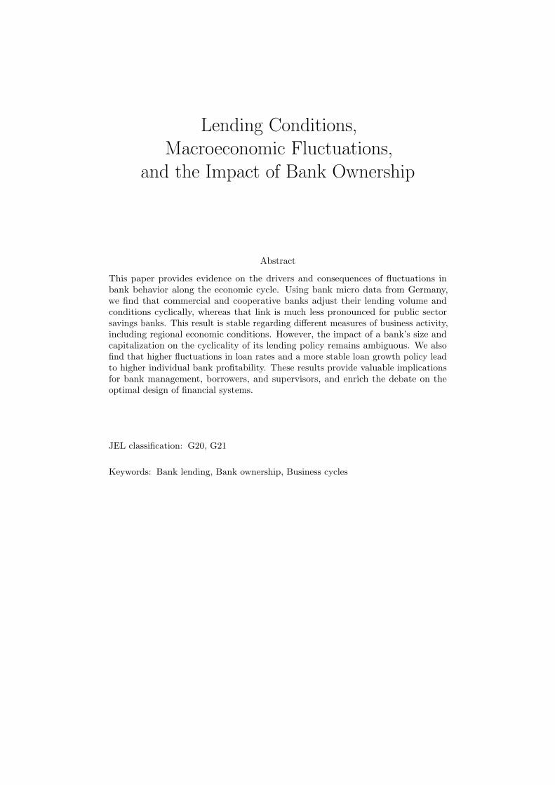
In a comparison of average volatility of bank behavior between commercial banks, coop-

eratives, and savings banks, the unbalanced nature of our panel may lead to distortions.

We therefore restrict this analysis to banks for which at least 17 observations are available,

which reduces the number of banks by 48.9%. The standard deviation of loan growth

(Panel A) and of the relative interest income (Panel B) is calculated from the time-series

for each of the 500 remaining banks. Box-plots show how these standard deviations are

distributed across banking sectors.

It turns out in Panel A of Figure 2 that, although mean loan growth rates are similar

for cooperatives and savings banks, banks in the latter group exhibit significantly less

variation in loan growth. As expected in H1, both cooperatives’ and savings banks’

lending activity fluctuates less than that of commercial banks. Evidence for the volatility

of the relative interest income in Panel B is less clear, but again, ‘average’ loan rates of

commercial banks fluctuate significantly more than those of cooperatives and savings

banks. This could however be related to the fact that the fraction of long-term loans is

lowest for commercial banks, allowing them to adjust loan rates at relatively short notice.

Please notice that the preceding analysis can only reveal how bank lending behavior

fluctuates in general, which may well be due to managerial decisions not systematically

related to the business cycle. Therefore, we propose the following multivariate model to

10

explain changes in loan growth of bank i in year t:

∆LGi,t = α+ β1∆GDPt + β2∆LGi,t−1 + β3∆RIIi,t + β4∆ETAi,t + β5∆LTLRt + εi,t

We believe that it is rather the change in the loan growth rate from the year t − 1 to

t than the actual growth rate that is determined by macroeconomic fluctuations and

therefore define our entire model in first differences. Thereby, we also implicitly control

for possible bank-specific fixed effects in our panel data set.

According to theory and the empirical literature, we expect a procyclical lending policy

and thus a positive coefficient for our main explanatory variable ∆GDPt. Additionally, we

include the lagged dependent variable ∆LGi,t−1, as it might be that loan growth exhibited

an unsystematic (positive or negative) shock in the preceding year, possibly due to the

introduction or the abolishment of new lending products or because of external bank

growth activity that our M&A criterion fails to detect. As we expect this unsystematic

effect to be reversed in the subsequent year, the coefficient β2 should be negative.

The change in the relative interest income ∆RIIi,t is included as control variable. On

one hand, it is more likely that a bank expands its lending when new, profitable lending

segments yielding relatively high loan rates are discovered. On the other hand, Foos

et al. (2007) report that loan growth could also have a negative impact on the relative

interest income, as banks may be underpricing their competitors to attract new customers.

Foos et al. (2007) also show that the equity-to-total assets ratio is negatively related to

loan growth, and we thus include changes in that ratio (∆ETAi,t) as additional control

variable. Finally, a high long term loan ratio (LTLRi,t) is obstructive for a bank to

adjust its lending cyclically. We control for changes in that ratio and expect it to be

negatively related with loan growth. Results from OLS regressions with Huber-White

robust standard errors, controlling for clustering at the individual bank-level, are reported

in Table 2.

11

Insert Table 2 here

Panel A compares regression results for our full sample with findings for each bank

group. First, as we expected, a positive and significant impact of GDP growth on loan

growth is confirmed. Our control variables also show their expected sign. Second, a

comparison of the estimated coefficients for commercial banks, cooperatives, and savings

banks leads to interesting results. It turns out that the link between GDP growth and

loan growth for savings banks is much less pronounced than for commercial banks or

cooperatives. Notice that the coefficient for cooperatives is 6 times higher than that for

savings banks,4 which is even more surprising as these banks are similar in many respect.

Furthermore, the loan growth of cooperatives seems to be more sensitive to the relative

interest income and to the long term loan ratio, whereas savings banks’ growth depends

to a higher degree on changes of the equity-to-total assets ratio. These results prove true

if we exclude banks for which less than 17 observations are available (quasi-balanced

panel), however for brevity, results are not presented here.

As we believe that a bank’s reaction to positive macroeconomic shocks may differ

from that to negative shocks, we restrict our analysis in Panel B of Table 2 to years

with accelerated economic growth (∆GDPt > 0) and in Panel C to years with weakened

economic growth (∆GDPt < 0). To obtain a homogeneous sample in these two panels,

only banks with at least 17 bank-year observations are analyzed. Our empirical results

show that the reaction on an economic improvement is substantially stronger than on

an economic slowdown. Aditionally, the pattern that savings banks tend to adjust their

lending less cyclically than cooperatives is confirmed for both differentiations. Hence, our

analyses until now strongly support Hypothesis H1 regarding savings banks’ cyclicality.

One problem with the linear regression model presented so far is that there may be

unobserved macroeconomic effects in some years which are not captured by GDP growth.

Therefore, we also test the link between fluctuations in lending and the economic cycle

4Tests as proposed by Chow (1960) confirm that coefficients are significantly distinct.

12

using the following fixed effects model for loan growth (LGi,t), which is similar to that

proposed by Micco and Panizza (2006):

LGi,t = α+ β1(SAVi ∗MACROt) + β2(COOPi ∗MACROt)

+ β3(SIZEi,t ∗MACROt) + β4(ETAi,t ∗MACROt) + γi + δt + εi,t

Indicator dummy variables for savings banks (SAVi) and cooperatives (COOPi) are

interacted with our main explanatory variable MACROt. Furthermore, we control

for bank size using the natural logarithm of total assets (SIZEi,t) as well as for bank

capitalization using the equity-to-total assets ratio (ETAi,t) and interact both variables

with MACROt. Fixed effects are included on a bank-specific (γi) and year-specific (δt)

level. Table 3 presents the empirical results.

Insert Table 3 here

For an interpretation of the coefficients from our fixed effects models, please notice that

the year-specific fixed effect captures the entire macroeconomic impact on the loan growth

rate in each year. We learned from our OLS regressions that loan growth generally shows

a procyclical behavior. Thus, if some explanatory variable causes the extent of cyclical

bank behavior to diminish, the coefficient of the interaction term should show a negative

sign, and vice versa. All regressions in Table 3 are estimated for the quasi-balanced panel

including only banks with at least 17 observations each.

Panel A uses the GDP growth rate as macroeconomic explanatory variable for loan

growth. The interaction terms with SAVi have a highly significant and negative coefficient,

meaning that savings banks indeed behave less cyclically. Furthermore, large banks and

banks with a lower equity-to-total assets ratio exhibit a slightly more cyclical lending

policy. These findings are robust for different specifications of control variables in

regression models 2 and 3.

13

In Panel B of table 3, we apply another macroeconomic variable, namely the ‘business

climate index’ of the economic situation in Germany provided by the Ifo Institute for

Economic Research at the University of Munich, as an early indicator of economic activity

in Germany. It could well be that the GDP growth rate used so far is a poor proxy for

the current state in the economic cycle due to its merely backward-looking definition.

Most importantly, all findings from Panel A are confirmed with this alternative measure

of business activity. Notice however that the explanatory power of the GDP growth

rate is substantially higher, as R-squares of the models in Panel A are almost 8 times

larger. Therefore, in our subsequent analyses, we prefer using the GDP growth rate as as

explanatory macro variable.5

Another important aspect of lending behavior is the cyclical adjustment of loan rates. If

it is indeed the case that savings banks and cooperatives commit to their customers in good

times as in bad, this should imply relatively constant loan rates over the macroeconomic

interest rate cycle. We model adjustments in the ‘average’ loan rate RIIi,t as follows:

∆RIIi,t = α+ β1∆INTERESTt + β2∆RIIi,t−1 + β3∆SIZEi,t + β4∆LGi,t

+ β5∆ETAi,t + β6∆IBLRi,t + β7LTLRi,t + εi,t

As are our regressions for the cyclicality of loan growth, this model is defined in first differ-

ences. The main explanatory variable is the macroeconomic interest rate INTERESTt,

for which we employ the 3-month interest rate (INT3Mt), or alternatively the 10-year

government bond yield (INT10t). Since a bank’s refinancing costs as well as the compet-

itive loan rate are strongly positively associated with the key interest rate, we expect

a positive impact on RIIi,t. The change in the lagged dependent variable RIIi,t−1 is

included as it is not unlikely that there is some serial correlation between changes in

loan rates. We further control for bank size using the natural logarithm of total assets

5One exception is the robustmess check using regional economic conditions in section 3.4.

14

(SIZEi,t) as well as for loan growth (LGi,t) and for the equity-to-total assets ratio

(ETAi,t). More importantly, the interbank loan ratio (IBLRi,t) should have a negative

impact on the relative interest income, as loan rates in interbank lending are typically

lower than those in customer lending. Moreover, a high long term loan ratio (LTLRi,t)

positively influences the average loan rate as long as there is a normal term structure

of interest rates, and we therefore expect a negative coefficient β7. Results from OLS

regressions are reported in Table 4

Insert Table 4 here

In Panel A, the 3-month interest rate is used as main explanatory variable. The expected

positive impact of the macroeconomic interest rate is confirmed for all banking groups,

and it turns out that the link between INT3Mt and the relative interest income RIIi,t is

significantly less pronounced for cooperatives and for savings banks than for commercial

banks.6 This is not exclusively driven by the higher average long term loan ratio of the

latter groups, as we firstly control for changes in that ratio in our regressions and secondly

obtain the same pattern when considering only commercial banks with high LTLRi,t as

reference group. Notice that there is indeed a positive serial correlation for changes in

the relative interest income. Furthermore, larger banks tend to have higher average loan

rates than smaller institutions. The coefficients for loan growth and the equity-to-total

assets ratio have very small values and are thus economically not significant. As expected,

a high fraction of interbank loans over total lending influences the relative interest income

negatively. Finally, only for cooperative banks, a positive impact of the long term loan

ratio on RIIi,t can be observed, which is consistent with our prediction. Summarizing, in

accordance with Hypothesis H1, cooperatives and savings banks adjust their loan rates

less cyclically.

Panel B uses 10-year government bond yields instead of short-term interest rates to

explain fluctuations in the ‘average’ loan rate. The findings of Panel A are confirmed6Tests as proposed by Chow (1960) confirm that coefficients are significantly distinct.

15

with two exceptions: Bank size is not significant any more, and the long term loan ratio

has a negative impact on the relative interest income, possibly because adjustments of

loan rates are not feasible at short notice if loan maturities are on average long.

Altogether, our analyses reveal that cooperative banks indeed adjust their loan rates

less cyclically than commercial banks, and public sector savings banks follow an even less

cyclical lending policy with regard to interest income as well as lending volume. Hence,

Hypothesis H1 is mainly supported by our empirical results.

3.2. Bank capitalization or size and the cyclicality of lending behavior

In the analyses in the preceding section, it remains open whether our findings are

exclusively driven by differences in ownership. It could well be that the on average

smaller size or better capitalization of cooperatives relative to savings banks is actually

responsible for their more cyclical behavior.

Therefore, we reconsider our baseline model from section 3.1 to explain changes in loan

growth and classify banks in each group into three size or capitalization terciles. Recall

that we hypothesized in H2 that better capitalized banks and smaller banks follow a less

cyclical lending policy.

Insert Table 5 here

Our analysis starts in Table 5 with a differentiation by size terciles for the full sample

(Panel A), cooperative banks (Panel B) and savings banks (Panel C). We calculate the

average size (total assets) for each bank over time and classify it into one of the models

1–3. No separate breakdown of commercial banks is conducted as their quite small

sub-samples (terciles) fail to provide significant results. For savings banks, it turns out

that the smallest tercile exhibits the strongest impact of GDP growth on loan growth,

which contradicts our proposition of less cyclicality due to a more direct bank-customer

relationship for these banks. Among cooperatives, the differentiation by bank size does

not lead to significantly different coefficients, and these are still four times higher than

16

for the smallest savings banks tercile. Thus, it is unlikely that the observed stronger

cyclicality of cooperative banks’ lending is solely driven by their on average smaller size.

Also, the size pattern in our full sample analysis (Panel A) mainly represents the

unobserved ownership characteristics, in particular the less pronounced cyclical behavior

of savings banks which are mostly classified into the mid oder even upper size tercile.

This is even more striking as our fixed effects models in Table 3 reveal a small, however

significantly positive impact of bank size on the cyclicality of lending, which is also in

line with our prediction in Hypothesis H2.

Insert Table 6 here

Table 6 reports the results regarding the impact of bank capitalization on the cyclicality

of loan growth. Again, banks are classified into terciles according to their average

equity-to-total assets ratio. Panel C shows that only savings banks with a relatively

good capitalization exhibit a significant link between GDP growth and loan growth. For

cooperatives (Panel B), which have on average a higher equity-to-total assets ratio, the

cyclicality of lending behavior is relatively homogeneous across capitalization terciles.

Notice again that the seemingly clear pattern in Panel A’s full sample analysis seems

to be mainly driven by ownership characteristics. Our findings from the fixed effects

models in Table 3 suggest that bank capitalization influences the cyclicality of lending

negatively, which is again consistent with Hypothesis H2. Notice also that Stolz and

Wedow (2005) observe the capital buffer of German savings and cooperative banks to

fluctuate anticyclically, which is more pronounced for savings banks. This could be a

consequence of their relatively stable lending behavior, inducing capital ratios to diminish

in bad times and to recover in economic upturns. Like for bank size, however, we cannot

find clear evidence for or against Hypothesis H2, which implies that bank ownership

turns out to be the dominant driver of more or less cyclical lending behavior.

17

3.3. Consequences of cyclical bank behavior

So far, we focused on the drivers of cyclicality in loan growth and loan rate setting.

However, from a systemic point of view, it is also interesting whether banks which behave

more cyclically gain profitability advantages. This proposition is not trivial as a stable or

even countercyclical lending policy could be helpful to establish durable bank-customer

relationships. These are very important in Germany’s (house) bank-based financial

system and may lead to economic rents, e.g. due to informational advantages.

Following this reasoning, it is clear that we should define bank profitability as an

average over the economic cycle, since the consequences of cyclicality in bank behavior

may only appear in the long run. Therefore, we propose the following regression model

for average profitability PROFi of bank i:

PROFi = α+ β1SD LGi + β2SD RIIi + β3SIZEi + β4ETAi

+ β5SAVi + β6COOPi + εi

The main explanatory variables are the standard deviations for each bank’s loan growth

SD LGi and relative interest income SD RIIt. Although these variables do not measure

whether fluctuations in lending behavior are linked to the economic cycle, they should

be suitable proxies for cyclicality in bank behavior. As control variables, the natural

logarithm of total bank assets (SIZEi) and the equity-to-total assets ratio (ETAi) are

added. Since existing papers report profitability (dis)advantages of savings banks and

cooperatives, we additionally include indicator dummy variables for these banking sectors

(SAVi and COOPi). Models are estimated as OLS regressions with robust standard

errors, coefficient estimates are displayed in Table 7.

Insert Table 7 here

A total of three alternative measures of average bank profitability PROFi are employed.

We use the relative net interest result RNIRi for our analyses in Panel A, the average

18

return on equity ROEt = operating result (t)average book equity (t−1,t) in Panel B, and the average return

on assets ROE = operating result (t)average total assets (t−1,t) in Panel C. The operating result is defined as

earnings from ordinary operations before taxes. It turns out that the standard deviation

of loan growth shows a negative impact on the bank’s return on equity, whereas its

coefficients in Panels A and C are statistically and/or economically not significant. This

means that a stable lending lending policy may also lead to profitability advantages.

However, we observe a positive and significant impact of the standard deviation of

‘average’ loan rates SD RIIi on the relative net interest result, indicating that it pays

for a bank to adjust loan rates cyclically. These findings are confirmed when controlling

for the possible multicollinearity between SD LGi and SD RIIi in models 2 and 3.

Coefficients for SIZEi are always significantly negative, which means that smaller

banks have profitability advantages over larger ones. Furthermore, banks with a higher

equity-to-total assets ratio ETAi exhibit on average a higher net interest result and

return on assets. This could however be due to the fact that these banks obtained a

better capitalization because of their higher profitability. Interestingly, our ownership

dummy variables both for savings and cooperative banks show insignificant coefficients

(with two exceptions), indicating that fundamental profitability (dis)advantages for these

banking groups do not exist.

These results have important implications from a systemic point of view. First and

most importantly, it is not bank ownership per se that drives its profitability. Also,

a relatively stable policy with regard to loan growth does not necessarily reduce bank

profitability, but influences a bank’s return on equity positively. However, our finding

that the average interest income fluctuates less for cooperatives and least for savings

banks could have a detrimental impact on interest margins. Thus, bank supervisors and

politicians have to weigh the provision of relatively stable lending conditions against the

advantage of more profitable savings banks. Notice that in a sense, the latter would also

improve the stability of the German financial system.

19

3.4. Robustness Checks

We complete the empirical analysis by testing our results for robustness with regard

to two aspects. First, as the activity of savings and cooperatives banks is restricted to

distinct geographic regions, it could be that they adjust their lending to regional economic

conditions rather than to the economic cycle for Germany. Second, savings banks and

cooperatives might behave less cyclically just because their management does not face

strong incentives to regularly adjust the lending policy, i.e. they do not intentionally

exhibit stable bank behavior but are rather ‘lazy’. This would contradict our proposition

that savings banks’ public mission of economic support and the commitment of credit

unions to support their cooperative members motivates their less cyclical lending policy.

Germany consists of 16 federal states, and most states are further divided into ad-

ministrative regions, so that we obtain 40 distinct regions for which economic data are

available for the period 1996–2005. We reconsider our baseline model from section 3.1 to

explain loan growth and substitute the GDP growth rate for Germany by the growth

rate of regional per-capita GDP (RGDPt). Regression results are reported in Table 8.

Insert Table 8 here

It turns out that for all three specifications, the entire sample period 1996–2005 in Panel

A, and years with accelerated (weakened) regional economic growth in Panel B (C),

the link of loan growth to regional economic conditions is less pronounced than to the

German GDP growth, as reported in Table 2. This could be due to higher unsystematic

fluctuations in regional economic activity adding too much noise in our main explanatory

variable which is hence unable to explain lending behavior properly. In any case, our

concern that savings and cooperative banks’ lending behavior could in fact be driven by

regional economic conditions is eliminated.

The issue of possibly ’lazy’ savings or cooperative banks is addressed by analyzing

other aspects of bank behavior except lending to customers. Specifically, we investigate

20

the deposit taking activity and the evolution of provision income over the economic

cycle. The first difference of the percentage change in total deposits from year t− 1 to t,

as well as the first difference in the growth of provision income are to be explained in

OLS regressions, where we apply again our baseline models from section 3.1. Coefficient

estimates are reported in Table 9.

Insert Table 9 here

Our empirical results suggest that the less cyclical behavior of savings banks and coop-

eratives is restricted to their lending activity. As Panel A documents, deposit taking

of banks shows a countercyclical pattern with negative coefficients. These are slightly

higher for commercial banks, however fundamental differences between cooperatives and

savings banks, that were prevalent in previous analyses, cannot be detected. Even more

striking are our results for the growth rate of provision income. Panel B shows that

this measure is by far more clearly associated with the economic cycle for savings and

cooperative banks. To sum up, these findings indicate that our observation of savings

banks and cooperatives ‘smoothing’ credit is essentially driven by the public mandate

of economic support and the commitment to cooperative members. This task affects

other bank activities to a lesser extent, so that a higher cyclicality of deposit taking and

provision income can well be observed.

4. Conclusions

This paper investigates the drivers and consequences of cyclical bank behavior. Using

data from more than 950 German banks over the period 1987–2005, three hypotheses on

the relation between bank ownership, bank size, bank capitalization, and the cyclicality of

lending behavior are tested. First, as we hypothesize in H1, loan growth and the average

loan rate of savings and cooperative banks fluctuates less. However, when analyzing the

link between these fluctuations and the business cycle, it turns out that the impact of

21

GDP growth on loan growth is similar in size for commercial banks and cooperatives, but

significantly less pronounced for public sector savings banks. This finding proves true

using different sample specifications and methodological approaches. Furthermore, we

find that savings banks and cooperatives indeed adjust their loan rates less cyclically than

commercial banks, which is consistent with savings banks’ public mission of economic

support and cooperative banks’ claim to commit to their clients in good times as in bad.

Second, we cannot detect a clear relation between a bank’s size or capitalization and

the cyclicality of its behavior, as H2 suggests. This finding supports our view that it is

indeed a bank’s ownership and not other possibly correlated characteristics that is the

driver of the less cyclical lending policy of savings banks and cooperatives. Third, our test

of H3 reveals that banks which show relatively stable loan growth rates over the economic

cycle exhibit higher returns on equity, whereas higher fluctuations in relative interest

income increase bank profitability via higher interest margins. Finally, robustness checks

verify that regional economic conditions do not drive savings and cooperative banks’

lending policy to a higher degree than does GDP growth for Germany, and that these

banks intentionally ‘smooth’ credit, which is not the case for other banking activities.

This paper has several implications. First, the ongoing debate about a necessary

restructuring in the German financial system is enriched by our finding that public sector

savings banks behave significantly less cyclically, which does not necessarily reduce their

profitability. Thus, they are an important factor for sustainable financial stability and

economic growth as they reliably provide financing for small and medium enterprizes.

Second, borrowers deciding about their financing sources should bear in mind our finding

that they can count on savings and cooperative banks rather than on private commercial

banks when economic conditions deteriorate. Finally, bank managers in Germany’s bank

(relationship)-based financial system should note that a more stable lending policy does

not essentially affect bank profitability negatively, however allows for the establishment

of durable bank-borrower relationships which may be beneficial for both sides.

22

References

Allen, Franklin, and Douglas Gale, 1999, Comparing Financial Systems (MIT Press).

Bernanke, Ben S., and Mark Gertler, 1995, Inside the black box: The credit channel of

monetary policy transmission., Journal of Economic Perspectives 9, 27–48.

Bichsel, Robert, 2006, State-Owned Banks as Competition Enhancers, or the Grand

Illusion, Journal of Financial Services Research 30, 117–150.

Bikker, Jacob A., and Haixia Hu, 2002, Cyclical Patterns in Profits, Provisioning, and

Lending of Banks, De Nederlandsche Bank Staff Report No. 86.

Chow, Gregory C., 1960, Tests of Equality Between Sets of Coefficients in Two Linear

Regressions, Econometrica 28, 591–605.

Delgado, Javier, Vicente Salas, and Jesus Saurina, 2007, Joint size and ownership

specialization in bank lending, Journal of Banking & Finance 31, 3563–3583.

Demirguc-Kunt, Asli, and Harry Huizinga, 1999, Determinants of Commercial Bank

Interest Margins and Profitability: Some International Evidence, World Bank Economic

Review 13, 379–408.

Elsas, Ralf, 2007, Preemptive distress resolution through bank mergers, Working Paper,

LMU Munich.

Fonteyne, Wim, 2007, Cooperative Banks in Europe - Policy Issues, IMF Working Paper

No. 07/159.

Foos, Daniel, Lars Norden, and Martin Weber, 2007, Loan Growth and Riskiness of

Banks, Working Paper, University of Mannheim.

Hackethal, Andreas, 2004, German banks and banking structure, in Jan P. Krahnen, and

Reinhard H. Schmidt, ed.: The German Financial System (Oxford University Press).

23

Hesse, Heiko, and Martin Cihak, 2007, Cooperative Banks and Financial Stability, IMF

Working Paper No. 07/02.

Iannotta, Giuliano, Giacomo Nocera, and Andrea Sironi, 2007, Ownership structure, risk

and performance in the European banking industry, Journal of Banking & Finance 33,

2127–2149.

International Monetary Fund, 2003, Germany: Financial System Stability Assessment,

IMF Country Report 03/343.

La Porta, Rafael, Florencio Lopez-de-Silanes, and Andrei Shleifer, 2002, Government

Ownership of Banks, Jounal of Finance 57, 265–301.

Levine, Ross, 2002, Bank-Based or Market-Based Financial Systems: Which Is Better?,

Journal of Financial Intermediation 11, 398 – 428.

Lown, Cara, and Donald P. Morgan, 2006, The Credit Cycle and the Business Cycle:

New Findings Using the Loan Officer Opinion Survey, Journal of Money, Credit, and

Banking 38, 1575 – 1597.

Micco, Alejandro, and Ugo Panizza, 2006, Bank ownership and lending behavior, Eco-

nomics Letters 93, 248 – 254.

, and Monica Yanez, 2007, Bank ownership and performance. Does politics

matter?, Journal of Banking & Finance 31, 219 – 241.

O’Hara, Maureen, 1981, Property rights and the financial firm, Journal of Law &

Economics 24, 317–332.

Quagliariello, Mario, 2007, Banks’ riskiness over the business cycle: a panel analysis on

Italian intermediaries, Applied Financial Economics 17, 119 – 138.

Rajan, Raghuram G., 1994, Why Bank Credit Policies Fluctuate: A Theory and Some

Evidence, Quarterly Journal of Economics 109, 399 – 441.

24

Sapienza, Paola, 2004, The effects of government ownership on bank lending, Journal of

Financial Economics 72, 357 – 384.

Smith, Donald J., Thomas F. Cargill, and Robert A. Meyer, 1981, An Economic Theory

of a Credit Union, Journal of Finance 36, 519–528.

Stolz, Stephanie, and Michael Wedow, 2005, Banks’ regulatory capital buffer and the busi-

ness cycle: evidence for German savings and cooperative banks, Deutsche Bundesbank

Banking and Financial Studies Discussion Paper No. 07/2005.

25

Figure 1: Macroeconomic variables during 1987–2005

This graph displays the development of our main macroeconomic variables during 1987–2005. Data onthe real GDP growth rate, the 3-month interest rate, and the 10-year government bond yield for Germanyare taken from OECD statistics.

23

45

67

89

10in

tere

st r

ates

−1

01

23

45

6G

DP

gro

wth

1987 1988 1989 1990 1991 1992 1993 1994 1995 1996 1997 1998 1999 2000 2001 2002 2003 2004 2005years

GDP growth 3 month interest 10 year interest

26

Figure 2: Standard deviation of bank behavior over the cycle

These Box-plots show how the standard deviation of each individual bank’s behavior differs within andacross bank groups. The standard deviation of loan growth (Panel A) and of the relative interest income(Panel B) over time is calculated for all banks with at least 17 observations (quasi-balanced panel).Loan growth is defined as the percentage change in total customer loans from the year t− 1 to t. Therelative interest income is measured as total interest income in year t over average loans in t− 1 and t inpercentage points.

Panel A: Standard deviation of loan growth

05

1015

Sta

ndar

d de

viat

ion

of lo

an g

row

th

Commercial Banks Cooperatives Savings Banksexcludes outside values

Panel B: Standard deviation of the relative interest income

01

23

Sta

ndar

d de

viat

ion

of r

elat

ive

inte

rest

inco

me

Commercial Banks Cooperatives Savings Banksexcludes outside values

27

Table 1: Summary statistics

Panel A: Representativeness of the sample

This panel compares the number of banks and the accumulated bank assets (in billion Euros) for the year2004 in our sample with the the respective statistics for Germany provided by the Deutsche Bundesbank.Notice that development banks, investment advisory firms, thrift institutions, branches of foreign banks,and other specialized banks (including Landesbanks and head institutions of cooperatives) are excludedboth from our sample and from Bundesbank statistics.

Number of banks (2004) Accumulated bank assets (2004)in sample in Germany coverage in sample in Germany coverage

Savings banks 386 477 80.9% 875bn 1,002bn 87.3%Cooperatives 324 1,336 24.2% 411bn 576bn 70.0%Comm. banks 56 252 22.2% 1,400bn 1,785bn 78.4%

Total 766 2,065 37.1% 2,686bn 3,364bn 79.8%

Panel B: Descriptive statistics for main variables

This panel displays the mean and standard deviation of our key variables for the full sample as well asdifferentiated by banking sectors. Total assets and total customer loans are denoted in billion Euros.

Full sample Comm. banks Cooperatives Savings banksMean St.Dev. Mean St.Dev. Mean St.Dev. Mean St.Dev.

Total assets (EUR) 2.29bn 15.2bn 11.4bn 47.6bn 0.89bn 3.65bn 1.63bn 1.88bnTotal customer loans (EUR) 1.28bn 7.4bn 5.98bn 23.2bn 0.54bn 1.89bn 0.98bn 1.18bnLoan growth 5.37% 6.53% 7.17% 9.68% 5.20% 7.25% 5.20% 5.18%Relative interest income 7.19% 1.39% 7.89% 2.44% 7.09% 1.31% 7.15% 1.20%Relative net interest result 1.98% 1.42% 3.32% 3.49% 2.19% 0.94% 1.62% 0.75%Equity-to-total assets ratio 4.99% 3.44% 8.40% 9.47% 5.01% 2.01% 4.36% 0.89%Fraction of long term loans 63.8% 17.1% 39.9% 23.0% 61.1% 14.2% 69.7% 13.4%Fraction of interbank loans 15.3% 10.1% 22.0% 17.2% 17.5% 8.8% 12.5% 8.0%

Number of observations 13,665 1,304 5,076 7,285Number of banks 959 94 382 483

28

Table 2: Regression results for the change in loan growth

The dependent variable is loan growth, defined as the first difference of the change in total customer loansfrom year t− 1 to t in percentage points: ∆LG = LGt − LGt−1. As main explanatory variable servesthe change in the GDP growth rate ∆GDP = GDPt −GDPt−1, again in percentage points. We controlfor the change in loan growth in the preceding year t− 1 and for bank characteristics, by including thefirst difference of the relative interest income (∆RII), the equity-to-total assets ratio (∆ETA), and thefraction of long-term loans over total customer loans (∆LTLR). The results reported in panels B and Care estimated using banks with at least 17 observations (quasi-balanced panel), differentiating for yearswith a positive or negative change in GDP growth. Huber-White robust standard errors, controllingfor clustering at individual banks, are reported in parentheses. ***, **, * indicate that coefficients arestatistically significant at the 1%, 5%, and 10%-level.

Panel A: Full sample period (1987–2005)

Full sample Comm. banks Cooperatives Savings banksCoeff. Std.Err. Coeff. Std.Err. Coeff. Std.Err. Coeff. Std.Err.

∆GDPt 0.355*** (0.410) 0.623** (0.265) 0.685*** (0.062) 0.117*** (0.039)∆LGi,t−1 -0.359*** (0.013) -0.401*** (0.038) -0.357*** (0.019) -0.337*** (0.018)∆RIIi,t 1.347*** (0.140) 0.463 (0.488) 2.167*** (0.221) 0.888*** (0.151)∆ETAi,t -1.557*** (0.261) -1.384*** (0.383) -0.980** (0.343) -2.492*** (0.376)∆LTLRi,t -2.410*** (0.537) -5.326** (2.406) -5.057*** (1.559) -0.925* (0.549)Constant -0.388*** (0.047) -0.646** (0.260) -0.289*** (0.148) -0.374*** (0.057)

# obs. 9,331 609 3,250 5,472# banks 891 79 347 465Adj. R2 0.160 0.199 0.186 0.132

Panel B: Years with accelerated economic growth (∆GDPt > 0)


∆GDPt 1.439*** (0.122) 0.345 (0.645) 2.247*** (0.223) 1.088*** (0.134)∆LGi,t−1 -0.336*** (0.030) -0.319*** (0.100) -0.342*** (0.040) -0.338*** (0.039)∆RIIi,t 0.834*** (0.218) 0.665* (0.829) 1.840*** (0.394) 0.042 (0.215)∆ETAi,t -2.066*** (0.566) -1.800* (1.067) -1.400 (0.850) -3.303*** (0.705)∆LTLRi,t -7.612*** (0.896) -5.452 (3.338) -15.17*** (2.500) -5.408*** (0.868)Constant -2.403*** (0.190) -1.032 (0.963) -3.321*** (0.361) -2.081*** (0.216)

# obs. 2,606 178 925 1,503# banks 498 44 188 266Adj. R2 0.168 0.143 0.184 0.172

Panel C: Years with weakened economic growth (∆GDPt < 0)


∆GDPt 0.586*** (0.095) 1.353* (0.730) 0.888*** (0.170) 0.310*** (0.102)∆LGi,t−1 -0.384*** (0.021) -0.460*** (0.062) -0.353*** (0.029) -0.390*** (0.026)∆RIIi,t 2.610*** (0.227) 0.320 (0.749) 2.899*** (0.423) 2.743*** (0.277)∆ETAi,t -1.847*** (0.378) -1.215** (0.542) -2.073*** (0.508) -2.960*** (0.531)∆LTLRi,t -5.816*** (1.174) -8.543 (11.81) -18.98** (8.232) -3.343*** (1.123)Constant 0.335** (0.148) 0.154 (0.913) 0.541** (0.272) 0.375** (0.176)

# obs. 3,706 262 1,320 2,214# banks 500 46 188 266Adj. R2 0.219 0.244 0.224 0.228

29

Table 3: Regression results for loan growth from fixed effects models

The dependent variable is loan growth, defined as the change in total customer loans from year t− 1 to tin percentage points. As main explanatory variable serves MACRO (alternatively the GDP growth rateor the difference of the average Ifo business climate index in years t− 1 and t), which we interact withindicator dummy variables for savings banks (SAV ∗MACRO) and cooperatives (COOP ∗MACRO).Additionally, the interaction terms for the natural logarithm of total assets (SIZE ∗MACRO) and forthe equity-to-total assets ratio (ETA ∗MACRO) are included as control variables, as well as bank andyear-specific fixed effects. Standard errors are reported in parentheses. ***, **, * indicate that coefficientsare statistically significant at the 1%, 5%, and 10%-level.

Panel A: MACRO = GDP growth (1987–2005)

Model 1 Model 2 Model 3Coeff. Std.Err. Coeff. Std.Err. Coeff. Std.Err.

SAVi ∗MACROt -1.094*** (0.233) -0.867*** (0.228) -1.052*** (0.241)COOPi ∗MACROt -0.287 (0.252) -0.040 (0.246) -0.348 (0.249)SIZEi,t ∗MACROt 0.118* (0.064) 0.151** (0.064)ETAi,t ∗MACROt -0.098* (0.051) -0.112** (0.051)Constant 8.701*** (1.182) 9.785*** (1.134) 6.719*** (0.397)Bank fixed effects yes yes yesYear fixed effects yes yes yes

# obs. 8,531 8,532 8,531# banks 501 501 501R2 0.238 0.235 0.235

Panel B: MACRO = Ifo business climate index (1991–2005)


SAVi ∗MACROt -0.264*** (0.090) -0.257*** (0.092) -0.242*** (0.094)COOPi ∗MACROt -0.008 (0.094) 0.008 (0.096) -0.023 (0.097)SIZEi,t ∗MACROt 0.031*** (0.007) 0.035*** (0.007)ETAi,t ∗MACROt -0.007*** (0.002) -0.008*** (0.003)Constant -32.85** (14.91) -50.21*** (17.99) 27.95*** (8.88)Bank fixed effects yes yes yesYear fixed effects yes yes yes

# obs. 7,097 7,098 7,097# banks 501 501 501R2 0.032 0.028 0.030

30

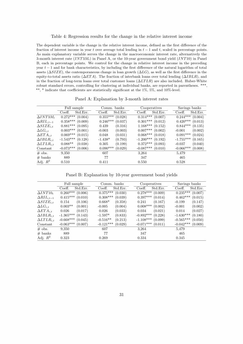
Table 4: Regression results for the change in the relative interest income

The dependent variable is the change in the relative interest income, defined as the first difference of thefraction of interest income in year t over average total lending in t− 1 and t, scaled in percentage points.As main explanatory variable serves the change in the macroeconomic interest rate, alternatively the3-month interest rate (INT3Mt) in Panel A, or the 10-year government bond yield (INT10) in PanelB, each in percentage points. We control for the change in relative interest income in the precedingyear t− 1 and for bank characteristics, by including the first difference of the natural logarithm of totalassets (∆SIZE), the contemporaneous change in loan growth (∆LG), as well as the first difference in theequity-to-total assets ratio (∆ETA). The fraction of interbank loans over total lending (∆IBLR), andin the fraction of long-term loans over total customer loans (∆LTLR) are also included. Huber-Whiterobust standard errors, controlling for clustering at individual banks, are reported in parentheses. ***,**, * indicate that coefficients are statistically significant at the 1%, 5%, and 10%-level.

Panel A: Explanation by 3-month interest rates


∆INT3Mt 0.272*** (0.004) 0.355*** (0.028) 0.314*** (0.007) 0.244*** (0.004)∆RIIi,t−1 0.358*** (0.009) 0.246*** (0.037) 0.301*** (0.012) 0.420*** (0.013)∆SIZEi,t 0.881*** (0.095) 0.439 (0.316) 1.168*** (0.152) 0.844*** (0.135)∆LGi,t 0.003*** (0.001) -0.003 (0.003) 0.007*** (0.002) -0.001 (0.002)∆ETAi,t 0.069*** (0.015) 0.048 (0.031) 0.068*** (0.018) 0.091*** (0.024)∆IBLRi,t -1.543*** (0.128) -1.438* (0.793) -1.200*** (0.192) -1.755*** (0.165)∆LTLRi,t 0.088** (0.038) 0.305 (0.199) 0.372*** (0.093) -0.037 (0.040)Constant -0.073*** (0.006) 0.090*** (0.029) -0.087*** (0.010) -0.066*** (0.008)

# obs. 9,350 607 3,264 5,479# banks 889 77 347 465Adj. R2 0.510 0.411 0.550 0.528

Panel B: Explanation by 10-year government bond yields


∆INT10t 0.260*** (0.006) 0.375*** (0.030) 0.278*** (0.009) 0.235*** (0.007)∆RIIi,t−1 0.415*** (0.010) 0.308*** (0.039) 0.397*** (0.014) 0.462*** (0.015)∆SIZEi,t 0.154 (0.106) 0.668* (0.358) 0.241 (0.167) -0.199 (0.147)∆LGi,t 0.003** (0.001) -0.005 (0.004) 0.008*** (0.002) -0.001 (0.002)∆ETAi,t 0.026 (0.017) 0.026 (0.033) 0.034 (0.021) 0.014 (0.027)∆IBLRi,t -1.365*** (0.143) -1.597* (0.833) -0.892*** (0.228) -1.630*** (0.180)∆LTLRi,t -0.668*** (0.045) -0.516** (0.213) -1.108*** (0.099) -0.565*** (0.050)Constant -0.063*** (0.007) -0.121*** (0.029) -0.071*** (0.011) -0.042*** (0.009)

# obs. 9,350 607 3,264 5,479# banks 889 77 347 465Adj. R2 0.323 0.269 0.334 0.345

31

Table 5: Impact of bank size on the cyclicality of loan growth

The dependent variable is loan growth, defined as the first difference of the change in total customer loansfrom year t− 1 to t in percentage points: ∆LG = LGt − LGt−1. As main explanatory variable servesthe change in the GDP growth rate ∆GDP = GDPt − GDPt−1, again in percentage points. Controlvariables are included as defined in Table 2. Panel A analyzes the full sample, whereas the observationsare restricted to cooperatives in Panel B and to savings banks in Panel C. Models 1–3 in each paneldifferentiate by terciles in banks’ average total assets. Huber-White robust standard errors, controllingfor clustering at individual banks, are reported in parentheses. ***, **, * indicate that coefficients arestatistically significant at the 1%, 5%, and 10%-level.

Panel A: Full sample, differentiated by size terciles

(1) Small banks (2) Mid banks (3) Large banksCoeff. Std.Err. Coeff. Std.Err. Coeff. Std.Err.

∆GDPt 0.564*** (0.109) 0.386*** (0.066) 0.195*** (0.053)∆LGi,t−1 -0.364*** (0.023) -0.346*** (0.022) -0.359*** (0.020)∆RIIi,t 1.630*** (0.311) 1.416*** (0.230) 1.038*** (0.203)∆ETAi,t -1.172*** (0.359) -1.739*** (0.423) -2.802*** (0.488)∆LTLRi,t -5.677*** (1.627) -0.502 (0.872) -2.375*** (0.719)Constant -0.430*** (0.100) -0.399*** (0.083) -0.271*** (0.068)

# obs. 2,129 3,385 3,791# banks 260 317 312Adj. R2 0.175 0.147 0.162

Panel B: Cooperative banks, differentiated by size terciles


∆GDPt 0.601*** (0.151) 0.731*** (0.130) 0.700*** (0.124)∆LGi,t−1 -0.304*** (0.036) -0.424*** (0.029) -0.320*** (0.028)∆RIIi,t 1.027** (0.444) 3.051*** (0.460) 2.305*** (0.405)∆ETAi,t -0.137 (0.796) -1.582*** (0.575) -1.867*** (0.718)∆LTLRi,t -5.720* (3.396) -5.676* (2.945) -3.595 (2.777)Constant -0.590*** (0.159) 0.130 (0.148) -0.133 (0.147)

# obs. 804 1,098 1,347# banks 98 125 124Adj. R2 0.128 0.255 0.169

Panel C: Savings banks, differentiated by size terciles


∆GDPt 0.172** (0.083) 0.124** (0.061) 0.064 (0.061)∆LGi,t−1 -0.285*** (0.037) -0.306*** (0.034) -0.395*** (0.023)∆RIIi,t 0.422 (0.265) 0.682*** (0.243) 1.319*** (0.248)∆ETAi,t -1.539*** (0.570) -2.076*** (0.598) -3.904*** (0.720)∆LTLRi,t -0.271 (1.033) -0.297 (0.815) -1.784* (0.961)Constant -0.612*** (0.106) -0.414*** (0.102) -0.158* (0.086)

# obs. 1,473 1,956 2,041# banks 143 162 160Adj. R2 0.093 0.098 0.197

32

Table 6: Impact of bank capitalization on the cyclicality of loan growth

The dependent variable is loan growth, defined as the first difference of the change in total customerloans from year t − 1 to t in percentage points: ∆LG = LGt − LGt−1. As main explanatory variableserves the change in the GDP growth rate ∆GDP = GDPt − GDPt−1, again in percentage points.Control variables are included as defined in Table 2. Panel A analyzes the full sample, whereas theobservations are restricted to cooperatives in Panel B and to savings banks in Panel C. Models 1–3 ineach panel differentiate by terciles in banks’ average equity-to-total assets (ETA) ratio. Huber-Whiterobust standard errors, controlling for clustering at individual banks, are reported in parentheses. ***,**, * indicate that coefficients are statistically significant at the 1%, 5%, and 10%-level.

Panel A: Full sample, differentiated by equity-to-total assets terciles

(1) Low ETA (2) Mid ETA (3) High ETACoeff. Std.Err. Coeff. Std.Err. Coeff. Std.Err.

∆GDPt 0.163*** (0.051) 0.241*** (0.051) 0.350*** (0.076)∆LGi,t−1 -0.458*** (0.023) -0.454*** (0.021) -0.509*** (0.024)∆RIIi,t 0.852*** (0.201) 1.556*** (0.180) 1.513*** (0.255)∆ETAi,t -2.599*** (0.507) -2.503*** (0.401) -1.525*** (0.316)∆LTLRi,t -1.492** (0.657) -2.519*** (0.836) -2.493** (1.074)Constant 2.457*** (0.158) 2.585*** (0.154) 2.650*** (0.176)

# obs. 3,573 3,894 3,117# banks 312 323 307Adj. R2 0.255 0.261 0.297

Panel B: Cooperative banks, differentiated by equity-to-total assets terciles


∆GDPt 0.537*** (0.091) 0.475*** (0.101) 0.459*** (0.142)∆LGi,t−1 -0.485*** (0.036) -0.484*** (0.030) -0.483*** (0.033)∆RIIi,t 1.600*** (0.362) 2.726*** (0.341) 2.296*** (0.481)∆ETAi,t -2.064*** (0.640) -0.438 (0.684) -0.621 (0.553)∆LTLRi,t -7.910*** (2.590) -5.007** (2.479) -3.808 (3.065)Constant 3.130*** (0.295) 2.517*** (0.228) 2.329*** (0.272)

# obs. 1,373 1,401 1,049# banks 126 128 125Adj. R2 0.280 0.326 0.288

Panel C: Savings banks, differentiated by equity-to-total assets terciles


∆GDPt -0.034 (0.080) 0.030 (0.050) 0.140*** (0.047)∆LGi,t−1 -0.482*** (0.028) -0.412*** (0.029) -0.430*** (0.033)∆RIIi,t 0.606** (0.250) 1.052*** (0.203) 0.456** (0.206)∆ETAi,t -2.824*** (0.718) -3.226*** (0.775) -3.236*** (0.561)∆LTLRi,t -1.218 (0.963) -0.770 (0.847) -1.254* (0.689)Constant 2.229*** (0.197) 2.339*** (0.220) 2.312*** (0.230)

# obs. 1,622 2,259 2,167# banks 158 164 160Adj. R2 0.286 0.219 0.235

33

Table 7: Impact of cyclical behavior on average bank profitability

The dependent variable is a bank profitability measure, alternatively the relative net interest income(RNII) in Panel A, the return on equity (ROE = operating income/book equity) in Panel B, or thereturn on assets (ROA = operating income/total assets) in Panel C. As main explanatory variable servethe standard deviation of loan growth (SD LG) and the standard deviation of the relative interest income(SD RII) for each bank. We control for bank size and capitalization by including the natural logarithm oftotal assets (SIZE) and the equity-to-total assets ratio (ETA). Additionally, indicator dummy variablesare included for Cooperative and Savings Banks. Huber-White robust standard errors are reported inparentheses. ***, **, * indicate that coefficients are statistically significant at the 1%, 5%, and 10%-level.

Panel A: Impact of cyclical behavior on the relative net interest result


SD LGi -0.005 (0.028) 0.004 (0.029)SD RIIi 1.059*** (0.198) 1.057*** (0.198)SIZEi -0.256*** (0.036) -0.268*** (0.041) -0.255*** (0.036)ETAi 0.089** (0.041) 0.072 (0.058) 0.089** (0.040)Coop. dummy 0.212 (0.202) -0.178 (0.242) 0.222 (0.215)Sav. dummy 0.006 (0.203) -0.478** (0.232) 0.023 (0.213)Constant 5.307*** (0.853) 7.307*** (1.067) 5.249*** (0.814)

# obs. 491 491 491Adj. R2 0.331 0.254 0.332

Panel B: Impact of cyclical behavior on the return on equity (ROE)


SD LGi -0.210*** (0.030) -0.213*** (0.030)SD RIIi 0.036 (0.242) -0.055 (0.246)SIZEi -0.105** (0.054) -0.121** (0.054) -0.068 (0.057)ETAi 0.001 (0.034) 0.002 (0.034) -0.007 (0.028)Coop. dummy -0.155 (0.297) -0.227 (0.279) 0.199 (0.315)Sav. dummy 0.127 (0.311) 0.061 (0.281) 0.864*** (0.310)Constant 6.864*** (1.327) 7.313*** (1.271) 4.567*** (1.395)

# obs. 490 491 490Adj. R2 0.190 0.191 0.089

Panel C: Impact of cyclical behavior on the return on assets (ROA)


SD LGi -0.009*** (0.002) -0.009*** (0.002)SD RIIi 0.019 (0.018) 0.016 (0.019)SIZEi -0.006* (0.003) -0.006* (0.004) -0.005 (0.004)ETAi 0.014** (0.006) 0.015*** (0.006) 0.014*** (0.005)Coop. dummy -0.022 (0.020) -0.027 (0.020) -0.007 (0.020)Sav. dummy -0.015 (0.019) -0.022 (0.018) 0.017 (0.019)Constant 0.276*** (0.082) 0.300*** (0.082) 0.177** (0.088)

# obs. 491 491 491Adj. R2 0.148 0.145 0.092

34

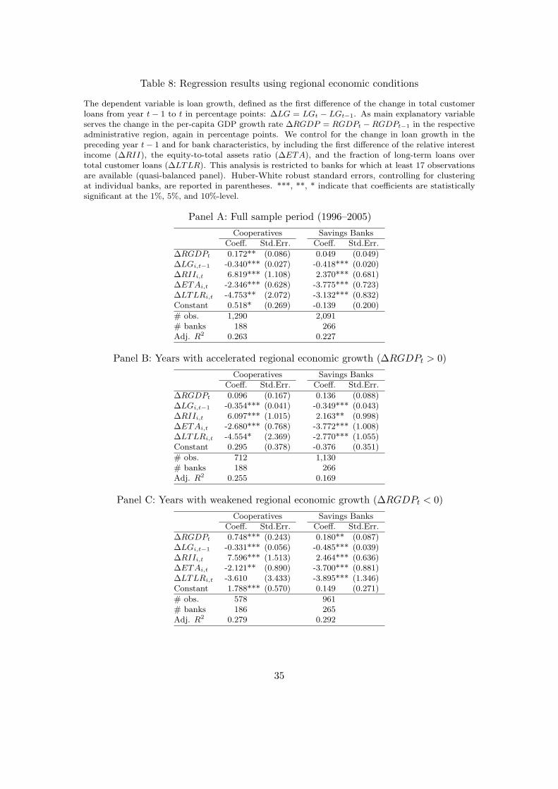
Table 8: Regression results using regional economic conditions

The dependent variable is loan growth, defined as the first difference of the change in total customerloans from year t − 1 to t in percentage points: ∆LG = LGt − LGt−1. As main explanatory variableserves the change in the per-capita GDP growth rate ∆RGDP = RGDPt −RGDPt−1 in the respectiveadministrative region, again in percentage points. We control for the change in loan growth in thepreceding year t− 1 and for bank characteristics, by including the first difference of the relative interestincome (∆RII), the equity-to-total assets ratio (∆ETA), and the fraction of long-term loans overtotal customer loans (∆LTLR). This analysis is restricted to banks for which at least 17 observationsare available (quasi-balanced panel). Huber-White robust standard errors, controlling for clusteringat individual banks, are reported in parentheses. ***, **, * indicate that coefficients are statisticallysignificant at the 1%, 5%, and 10%-level.

Panel A: Full sample period (1996–2005)

Cooperatives Savings BanksCoeff. Std.Err. Coeff. Std.Err.

∆RGDPt 0.172** (0.086) 0.049 (0.049)∆LGi,t−1 -0.340*** (0.027) -0.418*** (0.020)∆RIIi,t 6.819*** (1.108) 2.370*** (0.681)∆ETAi,t -2.346*** (0.628) -3.775*** (0.723)∆LTLRi,t -4.753** (2.072) -3.132*** (0.832)Constant 0.518* (0.269) -0.139 (0.200)

# obs. 1,290 2,091# banks 188 266Adj. R2 0.263 0.227

Panel B: Years with accelerated regional economic growth (∆RGDPt > 0)


∆RGDPt 0.096 (0.167) 0.136 (0.088)∆LGi,t−1 -0.354*** (0.041) -0.349*** (0.043)∆RIIi,t 6.097*** (1.015) 2.163** (0.998)∆ETAi,t -2.680*** (0.768) -3.772*** (1.008)∆LTLRi,t -4.554* (2.369) -2.770*** (1.055)Constant 0.295 (0.378) -0.376 (0.351)

# obs. 712 1,130# banks 188 266Adj. R2 0.255 0.169

Panel C: Years with weakened regional economic growth (∆RGDPt < 0)


∆RGDPt 0.748*** (0.243) 0.180** (0.087)∆LGi,t−1 -0.331*** (0.056) -0.485*** (0.039)∆RIIi,t 7.596*** (1.513) 2.464*** (0.636)∆ETAi,t -2.121** (0.890) -3.700*** (0.881)∆LTLRi,t -3.610 (3.433) -3.895*** (1.346)Constant 1.788*** (0.570) 0.149 (0.271)

# obs. 578 961# banks 186 265Adj. R2 0.279 0.292

35

Table 9: Cyclicality of deposit taking and the provision income

The dependent variable in Panel A is deposit growth, defined as the first difference of the change in totaldeposits from year t−1 to t in percentage points: ∆DEP = DEPt−DEPt−1. In Panel B, the dependentvariable is the percentage growth in total provision income, of which we also consider the first difference.As main explanatory variable serves the change in the GDP growth rate ∆GDP = GDPt − GDPt−1,again in percentage points. Control variables are included as defined in section 3.1. Additionally, changesin the long-term deposit ratio LTDEPRi,t, defined as the fraction of deposits with a maturity of morethan 5 years over total deposits, are considered. Huber-White robust standard errors, controlling forclustering at individual banks, are reported in parentheses. ***, **, * indicate that coefficients arestatistically significant at the 1%, 5%, and 10%-level.

Panel A: Impact of GDP growth on deposit growth


∆GDPt -0.662*** (0.042) -1.100*** (0.327) -0.529*** (0.077) -0.719*** (0.034)∆DEPGi,t−1 -0.439*** (0.012) -0.378*** (0.038) -0.454*** (0.017) -0.457*** (0.011)∆RIIi,t 1.689*** (0.167) 0.998 (0.647) 2.766*** (0.288) 1.010*** (0.160)∆ETAi,t -2.380** (1.013) -1.366 (1.078) -4.332*** (0.699) -3.953*** (0.373)∆LTDEPRi,t -0.097*** (0.018) -0.141*** (0.052) -0.062** (0.027) -0.103*** (0.014)Constant -0.068 (0.095) 0.152 (0.365) 0.353*** (0.104) -0.116** (0.053)

# obs. 9,618 620 3,409 5,589# banks 897 80 351 466Adj. R2 0.297 0.205 0.335 0.345

Panel B: Impact of GDP growth on the growth rate of provision income


∆GDPt 1.535*** (0.134) 0.288 (0.668) 1.316*** (0.299) 1.771*** (0.130)∆PROV Gi,t−1 -0.455*** (0.016) -0.464*** (0.044) -0.466*** (0.027) -0.437*** (0.020)∆SIZEi,t 12.03*** (4.107) 23.21** (10.70) 22.39*** (5.605) -17.16*** (4.698)∆ETAi,t 0.081 (0.313) 0.087 (0.360) 1.669** (0.755) -3.085*** (0.899)Constant -1.229*** (0.202) -0.367 (0.837) -1.713*** (0.336) 0.031 (0.248)

# obs. 9,633 704 3,331 5,598# banks 899 82 351 466Adj. R2 0.229 0.217 0.238 0.232

36

Documents

Lending Conditions, Macroeconomic Fluctuations, and the Impact of Bank ...€¦ · Lending Conditions, Macroeconomic Fluctuations, and the Impact of Bank Ownership Abstract This paper