Simulating cloud-aerosol interactions made by ship emissions

Lekha Patel* Lyndsay Shand∗

AbstractSatellite imagery can detect temporary cloud trails or ship tracks formed from aerosols emitted

from large ships traversing our oceans, a phenomenon that global climate models cannot directlyreproduce. Ship tracks are observable examples of marine cloud brightening, a potential solar cli-mate intervention that shows promise in helping combat climate change. Whether or not a ship’semission path visibly impacts the clouds above and how long a ship track visibly persists largelydepends on the exhaust type and properties of the boundary layer with which it mixes. In orderto be able to statistically infer the longevity of ship-emitted aerosols and characterize atmosphericconditions under which they form, a first step is to simulate, with mathematical surrogate modelrather than an expensive physical model, the path of these cloud-aerosol interactions with parame-ters that are inferable from imagery. This will allow us to compare when/where we would expectto ship tracks to be visible, independent of atmospheric conditions, with what is actually observedfrom satellite imagery to be able to infer under what atmospheric conditions do ship tracks form.In this paper, we will discuss an approach to stochastically simulate the behavior of ship inducedaerosols parcels within naturally generated clouds. Our method can use wind fields and potentiallyrelevant atmospheric variables to determine the approximate movement and behavior of the cloud-aerosol tracks, and uses a stochastic differential equation (SDE) to model the persistence behaviorof cloud-aerosol paths. This SDE incorporates both a drift and diffusion term which describes themovement of aerosol parcels via wind and their diffusivity through the atmosphere, respectively.We successfully demonstrate our proposed approach with an example using simulated wind fieldsand ship paths.

Key Words: Stochastic simulation atmospheric modeling, cloud-aerosol interactions, climate sci-ence, goes-r, state-space model.

*Statistical Sciences, Sandia National Laboratories, PO Box 5800 MS 1202, Albuquerque, NM 87185

arX

iv:2

111.

0535

6v1

[st

at.A

P] 9

Nov

202

1

1. Introduction

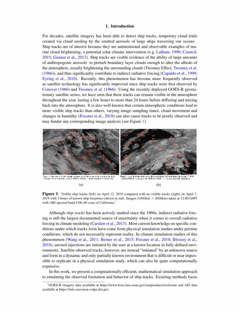
For decades, satellite imagery has been able to detect ship tracks, temporary cloud trailscreated via cloud seeding by the emitted aerosols of large ships traversing our oceans .Ship tracks are of interest because they are unintentional and observable examples of ma-rine cloud brightening, a potential solar climate intervention (e.g. Latham, 1990; Council,2015; Gunnar et al., 2013). Ship tracks are visible evidence of the ability of large amountsof anthropogenic aerosols to perturb boundary layer clouds enough to alter the albedo ofthe atmosphere, usually brightening the surrounding clouds (Twomey Effect, Twomey et al.(1966)), and thus significantly contribute to indirect radiative forcing (Capaldo et al., 1999;Eyring et al., 2010). Recently, this phenomenon has become more frequently observedas satellite technology has significantly improved since ship tracks were first observed byConover (1966) and Twomey et al. (1966). Using the recently deployed GOES-R geosta-tionary satellite series, we have seen that these tracks can remain visible in the atmospherethroughout the year, lasting a few hours to more than 24 hours before diffusing and mixingback into the atmosphere. It is also well-known that certain atmospheric conditions lead tomore visible ship tracks than others, varying image sampling times, cloud movement andchanges in humidity (Possner et al., 2018) can also cause tracks to be poorly observed andmay hinder any corresponding image analysis (see Figure 1).

(a) (b)

Figure 1: Visible ship tracks (left) on April 12, 2019 compared with no visible tracks (right) on April 7,2019 with 3 hours of known ship locations (shown in red). Images (5000km × 3000km) taken at 12:00 GMTwith ABI spectral band C06 off coast of California.1

Although ship tracks has been actively studied since the 1960s, indirect radiative forc-ing is still the largest documented source of uncertainty when it comes to overall radiativeforcing in climate modeling (Carslaw et al., 2013). Most current knowledge on specific con-ditions under which tracks form have come from physical simulation studies under pristineconditions, which do not necessarily represent reality. In climate simulation studies of thisphenomenon (Wang et al., 2011; Berner et al., 2015; Possner et al., 2018; Blossey et al.,2018), aerosol injections are initiated by the user at a known location in fully defined envi-ronments. Satellite-observed tracks, however, are instead “initiated” by an unknown sourceand form in a dynamic and only partially known environment that is difficult or near impos-sible to replicate in a physical simulation study, which can also be quite computationallyexpensive.

In this work, we present a computationally efficient, mathematical simulation approachto emulating the observed formation and behavior of ship tracks. Exisiting methods focus

1GOES-R imagery data available at https://www.bou.class.noaa.gov/saa/products/welcome and AIS dataavailable at https://info.seavision.volpe.dot.gov.

on modeling the chemical evolution of aerosol composition (Riemer et al., 2008; Sofievet al., 2009) and are not applicable to the physical modeling of cloud-aerosol paths throughthe atmosphere. Our approach aims to do so by flexibly accounting for the effect of weatherand atmospheric conditions.

Our method is different from physical simulation approaches in that it attempts to emu-late what is observed via satellite, rather than generate the full 3-D micro-physics environ-ment. Ultimately, we would like to infer from imagery and atmospheric data under whatconditions do track form or not form to incorporate in our emulation approach. For now,without more information on to what degree atmospheric conditions effect the visibility orbehavior, we present the general framework accounting for the cloud movement and pointout where atmospheric effects can be incorporated.

The remainder of this paper is organized as follows: Section 2 presents the backgroundmotivating the simulations. Section 3 and 4 outlines our emulation approach and providessimulation examples, respectively. Lastly, Section 5 discusses follow-on work and potentialimpacts of this research.

2. Background

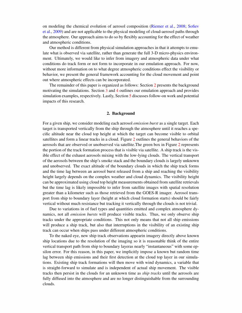
For a given ship, we consider modeling each aerosol emission burst as a single target. Eachtarget is transported vertically from the ship through the atmosphere until it reaches a spe-cific altitude near the cloud top height at which the target can become visible to orbitalsatellites and form a linear tracks in a cloud. Figure 2 outlines the general behaviors of theaerosols that are observed or unobserved via satellite.The green box in Figure 2 representsthe portion of the track formation process that is visible via satellite. A ship track is the vis-ible effect of the exhaust aerosols mixing with the low-lying clouds. The vertical transportof the aerosols between the ship’s smoke stack and the boundary clouds is largely unknownand unobserved. The exact altitude of the boundary clouds in which the ship track formsand the time lag between an aerosol burst released from a ship and reaching the visibilityheight largely depends on the complex weather and cloud dynamics. The visibility heightcan be approximated using cloud top height measurements obtained from satellite retrievalsbut the time lag is likely impossible to infer from satellite images with spatial resolutiongreater than a kilometer such as those retrieved from the GOES-R imager. Aerosol trans-port from ship to boundary layer (height at which cloud formation starts) should be fairlyvertical without much resistance but tracking it vertically through the clouds is not trivial.

Due to variations in of fuel types and quantities emitted and complex atmosphere dy-namics, not all emission bursts will produce visible tracks. Thus, we only observe shiptracks under the appropriate conditions. This not only means that not all ship emissionswill produce a ship track, but also that interruptions in the visibility of an existing shiptrack can occur when ships pass under different atmospheric conditions.

To the naked eye, new ship track observations appearin imagery directly above knownship locations due to the resolution of the imaging so it is reasonable think of the entirevertical transport path from ship to boundary layeras nearly “instantaneous” with some ep-silon error. For this reason, in this paper, we implicitly impose a known but random timelag between ship emissions and their first detection at the cloud top layer in our simula-tions. Existing ship track formations will then move with wind dynamics, a variable thatis straight-forward to simulate and is independent of actual ship movement. The visibletracks then persist in the clouds for an unknown time as ship tracks until the aerosols arefully diffused into the atmosphere and are no longer distinguishable from the surroundingclouds.

Figure 2: https://ral.ucar.edu/staff/jwolff/aerosols.html/intro.html

3. Modeling aerosols using a Hidden Markov Model (HMM)

To model the formation and behavior of the aerosol tracks we construct a state-space pointprocess representation relating imaging observations of emission tracks to partially ob-served, known locations of aerosol emission bursts from ships. A constructed HiddenMarkov Model (HMM) is outlined sectionto characterize the relationship between betweenthe image observations and partially observed truth. We are interested in building a com-putational model that can emulate the persisting behavior the ship tracks to understand howthis behavior changes with changing atmospheric dynamics.

3.1 State-space representation

The true emission path is generated by the continuously emitted aerosol emission packetsby a single ship over the spatial window X ⊂ R2 up to time T ∈

[0,∑N−1

n=1 ∆n,n+1

]where N is the number of frames and ∆n,n+1 > 0 is the time between frames n andn + 1 (typically between 5 and 15 minutes). For simplicity, we assume in this article that∆n,n+1 ≡ ∆, so that tn+1 − tn = ∆ for all n.

We first define the unobserved spatio-temporal point process {Xn : (x, y, tn) ∈ R2 ×R} which characterizes the true behavior of the aerosol emission bursts, continuously re-leased prior to (and still visible at) time tn. Second, we define the observed spatio-temporalpoint process {Yn : (x, y, t) ∈ R2 × R} which characterizes the patterns of the partiallyobserved ship tracks in image frame n, generated by Xn. Using this state-space represen-tation, we formulate a Hidden Markov Model relating the two processes. T can also bedefined in terms of number of image frames such that T ∈

[0,∑N−1

n=1 ∆n,n+1

]where N

is the number of frames and ∆n,n+1 > 0 is the time between frames n and n + 1. Forsimplicity, and since many imagers tend to collect data at regular intervals, we assume that∆n,n+1 ≡ ∆, so that tn+1 − tn = ∆ for all n.

The true emission path is generated by the continuously emitted aerosol emission pack-ets by a single ship over the spatial window X ⊂ R2 up to time T > 0, T ∈ R, with X andtime T typically defined by the imager or the user. Although in practice, the observed satel-lite imagery and our partially observed data Ytn is observed discreetly, we will treat timeas continuous in our simulation model. For ship k = 1 . . .K which produces a track, weassume that its entire emission path is comprised of Pk > 0 aerosol bursts(packets) whichmay or may not become visible. Assuming that only ktn of K ships that are expected tobe observed prior to T , have entered the window X by time tn < T , for an arbitrary singletrack k = 1 . . . ktn , only pktn ≤ Pk packets are expected to become visible. To show proof

of concept, for now we will ignore the complex cloud dynamics and assume all emissionpackets reach reach the boundary layer clouds and become visible with time lag < ε. Thiswill allow us to start with a general simulation framework and build in more atmosphericconditions when needed at a later time.

In the region of interest X , we denote the set of true positions or states of each packetas {xi,n}

pktni=1 , where xi,n ∈ X denotes the state of the ith packet of emission track k at

time tn.Existing ship tracks are only modified at the next time step tn+1 in three possible ways:

• the oldest aerosol emission packets at the end of the track diffuse completely and mixback into the atmosphere (leaving no detectable trace), or

• surviving packets diffuse and become less distinguishable as part of the track (but arestill visible), according to cloud dynamics and wind motion, or

• new packets appear at the front of the track in the direction the ship movement.

These situations result in pkn+1 new states(locations) {xi,tn+1}pkn+1

i=1 in each of the newand existing emission tracks present at time tn+1.

In practice, however, the full lifespan (from first appearance to permanent disappear-ance) of each emission packet is unknown. Instead, at each observed image frame n, theGOES-R ABI sensor captures a snapshot in time of all estimated packet locations withoutinformation on age of the packet, i.e. how long the observations have visibly persisted inthe atmosphere. It is also the case that the locations of the emission packets over theirlifespan are not unique and can share a location with another emission packet. Specifically,for a track ktn , a set of oktn ≤ pktn observations {yi,tn}

oktni=1 , is recorded, where yi,tn ∈ Y

denotes the state of the ith observation at time tn. We may assume that Y = X .At time tn ∈ R, a newly observed track can be generated from newly released emission

packets into the atmosphere. Due to the complex dynamics of the atmosphere, it is notoften possible to link new observations to their true source. An observed aerosol trackfrom GOES-R is not always visible directly above the known ship location. Thus, wewill assume that there is no information about which emission packet generates whichobservation. Since there is no ordering on the respective collections of emission packetstates and measurements at time tn, they can be naturally represented as finite spatial-temporal point processes. Specifically, for n = 1, . . . N , we denote

Xtn = {{x1,tn , . . . ,xp1,tn︸ ︷︷ ︸p1 packets

from emission 1

}, . . . , {xktn ,tn , . . . ,xpktn ,tn︸ ︷︷ ︸pktn packets

from emission ktn

}} ∈ F(X ) ktn ≤ K

Ytn = {{y1,tn , . . . ,yo1,tn︸ ︷︷ ︸o1 packets

from emission 1

}, . . . , {yktn ,tn , . . . ,yoktn ,tn︸ ︷︷ ︸oktn packets

from emission ktn

}} ∈ F(Y) 0 ≤ on ≤ pktn

where F(X ) and F(Y) denote the collections of all finite subsets of X and Y respectively.The target point process Xtn is referred to as the multi-target state and the measurementset Ytn is referred to as the multi-target observation. With this model specification, theobjective is to recover the true states of emission packet point processes Xt1 , Xt2 , . . . , XtN

from their measurement sets Yt1 , Yt2 , . . . , YtN .

3.1.1 Multi-target state model

In this section, we describe a finite point process model for the time evolution of themultiple-target state Xtn , n = 1, . . . , N , which incorporates emission packet motion, birth

and death. Specifically, we mathematically define the processes of aerosol packets first be-ing conceived in boundary layer clouds, their motion and diffusion through the atmosphereuntil their permanent disappearance.

After an aerosol track has already formed at time tn−1, if an emission packet xtn−1 ∈Xtn−1 which makes up part of that track survives to time tn+1 > tn, its subsequent state isdetermined by a drift term which is described by the wind motion at xtn−1 , and a diffusionterm which describes the diffusion of the emission packet within the clouds it is situatedin. This type of process is known as a Markov diffusion process and is described by thefollowing (continuous time) stochastic differential equation:

dxt = µ(xt, t)︸ ︷︷ ︸drift

dt+ σ(xt, t)︸ ︷︷ ︸diffusion

dBt, (1)

where Bt ∼ N2(0, tI2) denotes a standard Brownian motion in two dimensions, with I2

denoting the 2-dimensional identity matrix. The drift function µ(xt) denotes the windvelocity at point xt, at time t and is in general known. For this problem, we choose thediffusion function σ(xt) ≡ σx to be a constant that describes the diffusivity of an aerosolparcel within the atmospheric boundary layer. The solution to (1) with a changing windvelocity in space and time is in general unknown and requires numerical solvers whichmay be computationally cumbersome and time consuming. For simulation purposes, wetherefore propose the following approximation.

Given discrete time intervals of the form In = (tn, tn+1] ≡ (n∆, (n + 1)∆], withn ∈ Z+, we assume that the simulation interval time tn+1 − tn = ∆ is taken small enoughso that the wind velocity within the interval is approximately constant. That is to say, for acontinuous time point t ∈ In, we use the approximate SDE

dxt = µ(xt)dt+ σxdBt, (2)

with µ(xt) denoting the wind velocity field for a parcel with state xt. Given a previousstate xs at time s ∈ In, t > s, equation (1) can be solved directly

dxt = µ(xt)dt+ σxdBt

=⇒ xt − xs =

∫ t

sµ(xt) dw + σx(Bt −Bs)

= µ(xt)(t− s) + σxBt−s,

where Bt − BsD≡ 2Bt−s ∼ N2(0, (t − s)I2). This implies the corresponding transition

density isxt|xs ∼ N2(xs + µ(xs)(t− s), σ2

x(t− s)I2).

In particular, the probability density of the parcel’s transition to state xtn ∈ Xtn from statextn−1 is given by the Markovian density fMtn|tn−1

(xtn |xtn−1) ∼ N2(xtn−1+µ(xtn−1)∆, σ2x∆I2).

Its behavior at this time is therefore modeled by the point process Stn|tn−1(xtn−1), where

Stn|tn−1(xtn−1) =

{xtn where xtn ∼ fMtn|tn−1

(·|xtn−1) with probability pS,tn(bxtn−1)

∅ otherwise.(3)

Here, pS,tn(bxtn−1) denotes the survival probability of packet xtn−1at time tn (described in

more detail below) and where the motion diffusion coefficient σx is unknown and requiresestimation from the model.

2D≡ denotes equivalence in distribution.

A new emission packet at time tn ∈ R can arise in two ways. The first is as a sponta-neous birth (of a newly risen emission track), which is independent of any existing emissiontrack. The second is by spawning from an existing emission source, resulting in a newlyvisible emission packet. We denote the birth time of packet xtn (partially) observed at timetn as bxtn .

Spontaneous births of new emission tracks at time t are denoted by the finite pointprocess Γt. We model Γt as a finite Poisson point process with intensity function γt(x) =λγtfb,t(x)), for x ∈ X :

Γt ∼ Poisson(λγtfb,t(x)). (4)

• Here, Nb,t ∼ Poisson(∫X λγtfb,t(x)dx) denotes the number of births occurring in X

at time t.

• fbt(x) denotes their spatial distribution.

Assuming we have knowledge (simulated or real) of the boat positions/path that producethese new emissions, we may let this inform fbt(x). Specifically, if xb,tn is the positionof a new boat at time tn, then fbtn+ε(x) = N2(xb,tn , σ

2b I2) where ε denotes the time lag

between ship emission and aerosol observation at the cloudboundary layer.Spawned births occurring within the time interval In−1 denote newly visible emission

packets from existing emission tracks that reach the cloud top layer at time tn. Newlyspawned targets can only be spawned by packets that were birthed in the previous timeinterval In−2, as this models the continuous emission of aerosol packets in a single stream.

We model the set of spawned births Btn|tn−1(xtn−1) at time tn from a packet xtn−1

at time tn−1 as a finite point process. An example used in this paper is Bernoulli pointprocess with spawning probability pβ,tn :

Btn|tn−1(xtn−1) =

{{x}; x ∼ fβtn|tn−1

(x|xtn−1) with probability pβ,tn tn−2 < bxtn−1≤ tn−1

∅ otherwise.

1. The number of spawned targets Ns,tn from xtn−1 follows Ns,tn ∼ Bernoulli(pβ,tn).

2. Therefore at most one packet can be spawned from a target xtn−1 born in the previoustime step.

3. IfNs,tn = 1, then the spatial distribution of the spawned target x follows fβtn|tn−1(·|xtn−1)

from xtn−1 .

In this paper, we assume knowledge of ship positions that continuously emit aerosolswhilst moving, thereby corresponding to this spawning process. For simulation purposes,we therefore use the spawning density

fβtn|tn−1(x|xtn−1) = N2(xb,tn−ε + εσ2

βI2).

The spawning probability pβ,tn is directly related to the number of aerosol packets eachship emits during the observed time window. For simulation purposes, we assume that eachboat continuously emits aerosols up to the simulation time T = N∆ and that they existwhen within the observed window X . This enables pβ,tn = 1 when tn ≤ T and is zerootherwise.

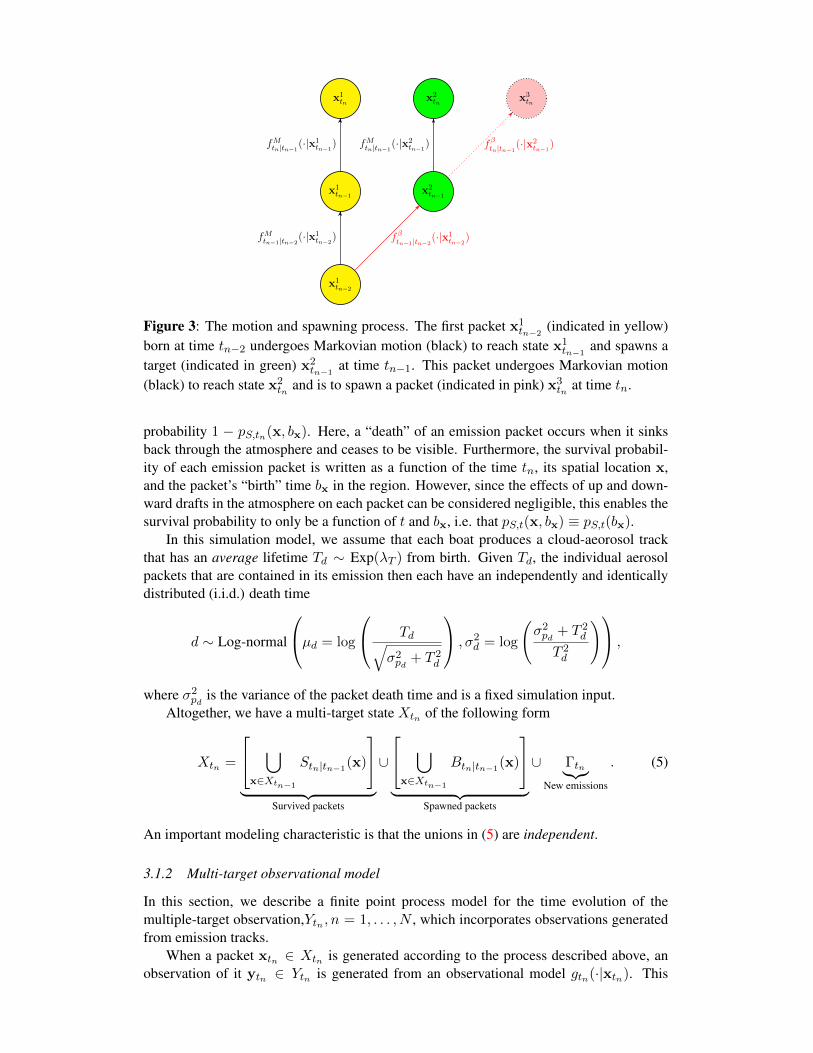
Figure 3 illustrates the motion and spawning process of an aerosol packet described byour procedure.

For a given multi-target state Xtn−1 at time tn−1, each packet x ∈ Xtn−1 either con-tinues to exist (survives) at time tn > tn−1 with probability pS,tn(x, bx), or “dies” with

x1tn−2

x1tn−1

x1tn

x2tn−1

x2tn x3

tn

fMtn−1|tn−2(·|x1

tn−2)

fMtn|tn−1(·|x1

tn−1) fMtn|tn−1

(·|x2tn−1

)

fβtn−1|tn−2(·|x1

tn−2)

fβtn|tn−1(·|x2

tn−1)

Figure 3: The motion and spawning process. The first packet x1tn−2

(indicated in yellow)born at time tn−2 undergoes Markovian motion (black) to reach state x1

tn−1and spawns a

target (indicated in green) x2tn−1

at time tn−1. This packet undergoes Markovian motion(black) to reach state x2

tn and is to spawn a packet (indicated in pink) x3tn at time tn.

probability 1 − pS,tn(x, bx). Here, a “death” of an emission packet occurs when it sinksback through the atmosphere and ceases to be visible. Furthermore, the survival probabil-ity of each emission packet is written as a function of the time tn, its spatial location x,and the packet’s “birth” time bx in the region. However, since the effects of up and down-ward drafts in the atmosphere on each packet can be considered negligible, this enables thesurvival probability to only be a function of t and bx, i.e. that pS,t(x, bx) ≡ pS,t(bx).

In this simulation model, we assume that each boat produces a cloud-aeorosol trackthat has an average lifetime Td ∼ Exp(λT ) from birth. Given Td, the individual aerosolpackets that are contained in its emission then each have an independently and identicallydistributed (i.i.d.) death time

d ∼ Log-normal

µd = log

Td√σ2pd

+ T 2d

, σ2d = log

(σ2pd

+ T 2d

T 2d

) ,

where σ2pd

is the variance of the packet death time and is a fixed simulation input.Altogether, we have a multi-target state Xtn of the following form

Xtn =

⋃x∈Xtn−1

Stn|tn−1(x)

︸ ︷︷ ︸

Survived packets

∪

⋃x∈Xtn−1

Btn|tn−1(x)

︸ ︷︷ ︸

Spawned packets

∪ Γtn︸︷︷︸New emissions

. (5)

An important modeling characteristic is that the unions in (5) are independent.

3.1.2 Multi-target observational model

In this section, we describe a finite point process model for the time evolution of themultiple-target observation,Ytn , n = 1, . . . , N , which incorporates observations generatedfrom emission tracks.

When a packet xtn ∈ Xtn is generated according to the process described above, anobservation of it ytn ∈ Ytn is generated from an observational model gtn(·|xtn). This

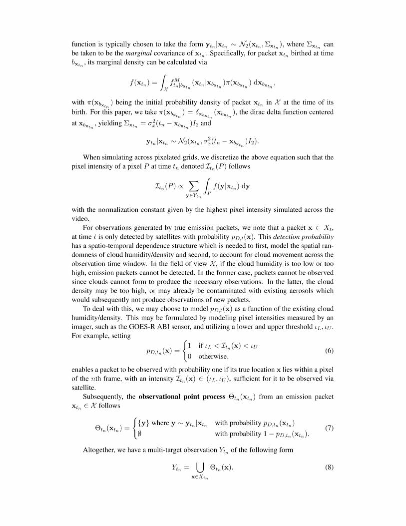
function is typically chosen to take the form ytn |xtn ∼ N2(xtn ,Σxtn ), where Σxtn canbe taken to be the marginal covariance of xtn . Specifically, for packet xtn birthed at timebxtn , its marginal density can be calculated via

f(xtn) =

∫XfMtn|bxtn

(xtn |xbxtn )π(xbxtn ) dxbxtn ,

with π(xbxtn ) being the initial probability density of packet xtn in X at the time of itsbirth. For this paper, we take π(xbxtn ) = δxbxtn

(xbxtn ), the dirac delta function centered

at xbxtn , yielding Σxtn = σ2x(tn − xbxtn )I2 and

ytn |xtn ∼ N2(xtn , σ2x(tn − xbxtn )I2).

When simulating across pixelated grids, we discretize the above equation such that thepixel intensity of a pixel P at time tn denoted Itn(P ) follows

Itn(P ) ∝∑

y∈Ytn

∫Pf(y|xtn) dy

with the normalization constant given by the highest pixel intensity simulated across thevideo.

For observations generated by true emission packets, we note that a packet x ∈ Xt,at time t is only detected by satellites with probability pD,t(x). This detection probabilityhas a spatio-temporal dependence structure which is needed to first, model the spatial ran-domness of cloud humidity/density and second, to account for cloud movement across theobservation time window. In the field of view X , if the cloud humidity is too low or toohigh, emission packets cannot be detected. In the former case, packets cannot be observedsince clouds cannot form to produce the necessary observations. In the latter, the clouddensity may be too high, or may already be contaminated with existing aerosols whichwould subsequently not produce observations of new packets.

To deal with this, we may choose to model pD,t(x) as a function of the existing cloudhumidity/density. This may be formulated by modeling pixel intensities measured by animager, such as the GOES-R ABI sensor, and utilizing a lower and upper threshold ιL, ιU .For example, setting

pD,tn(x) =

{1 if ιL < Itn(x) < ιU

0 otherwise,(6)

enables a packet to be observed with probability one if its true location x lies within a pixelof the nth frame, with an intensity Itn(x) ∈ (ιL, ιU ), sufficient for it to be observed viasatellite.

Subsequently, the observational point process Θtn(xtn) from an emission packetxtn ∈ X follows

Θtn(xtn) =

{{y} where y ∼ ytn |xtn with probability pD,tn(xtn)

∅ with probability 1− pD,tn(xtn).(7)

Altogether, we have a multi-target observation Ytn of the following form

Ytn =⋃

x∈XtnΘtn(x). (8)

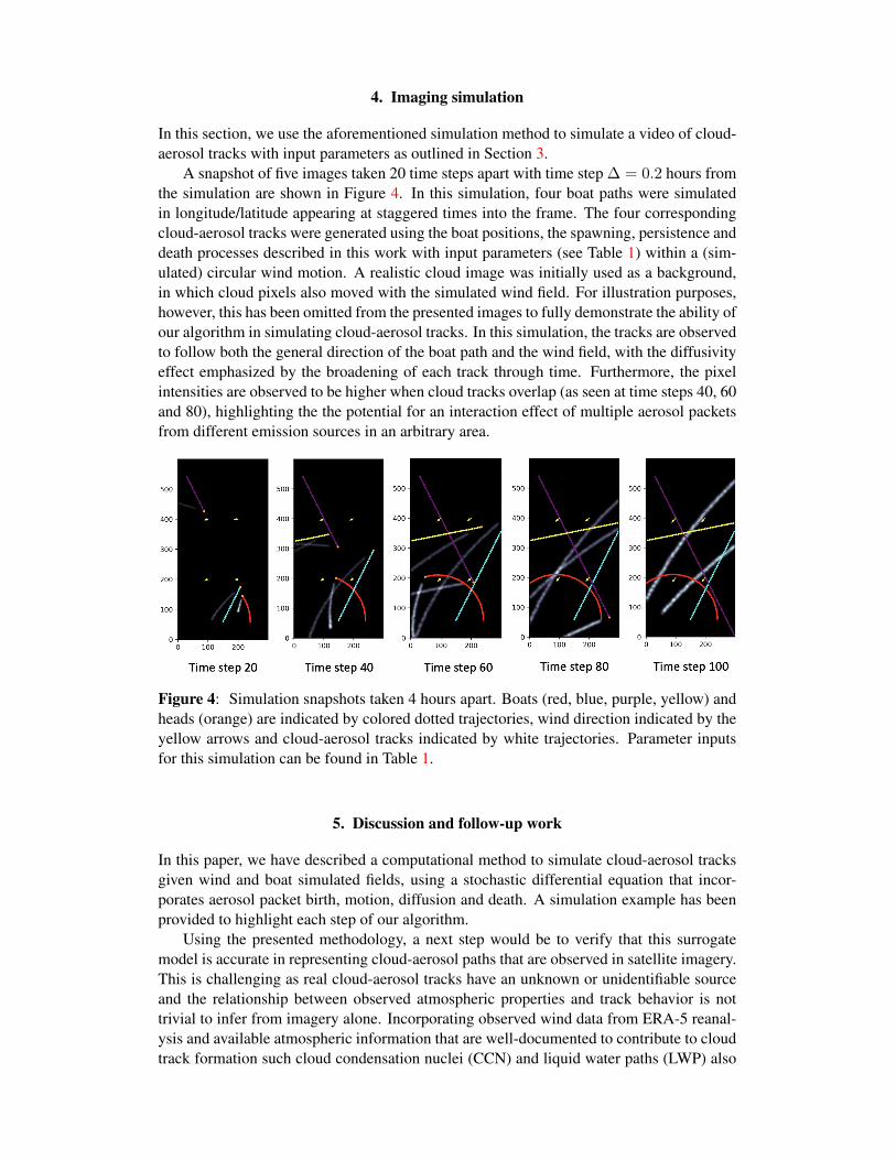
4. Imaging simulation

In this section, we use the aforementioned simulation method to simulate a video of cloud-aerosol tracks with input parameters as outlined in Section 3.

A snapshot of five images taken 20 time steps apart with time step ∆ = 0.2 hours fromthe simulation are shown in Figure 4. In this simulation, four boat paths were simulatedin longitude/latitude appearing at staggered times into the frame. The four correspondingcloud-aerosol tracks were generated using the boat positions, the spawning, persistence anddeath processes described in this work with input parameters (see Table 1) within a (sim-ulated) circular wind motion. A realistic cloud image was initially used as a background,in which cloud pixels also moved with the simulated wind field. For illustration purposes,however, this has been omitted from the presented images to fully demonstrate the ability ofour algorithm in simulating cloud-aerosol tracks. In this simulation, the tracks are observedto follow both the general direction of the boat path and the wind field, with the diffusivityeffect emphasized by the broadening of each track through time. Furthermore, the pixelintensities are observed to be higher when cloud tracks overlap (as seen at time steps 40, 60and 80), highlighting the the potential for an interaction effect of multiple aerosol packetsfrom different emission sources in an arbitrary area.

Figure 4: Simulation snapshots taken 4 hours apart. Boats (red, blue, purple, yellow) andheads (orange) are indicated by colored dotted trajectories, wind direction indicated by theyellow arrows and cloud-aerosol tracks indicated by white trajectories. Parameter inputsfor this simulation can be found in Table 1.

5. Discussion and follow-up work

In this paper, we have described a computational method to simulate cloud-aerosol tracksgiven wind and boat simulated fields, using a stochastic differential equation that incor-porates aerosol packet birth, motion, diffusion and death. A simulation example has beenprovided to highlight each step of our algorithm.

Using the presented methodology, a next step would be to verify that this surrogatemodel is accurate in representing cloud-aerosol paths that are observed in satellite imagery.This is challenging as real cloud-aerosol tracks have an unknown or unidentifiable sourceand the relationship between observed atmospheric properties and track behavior is nottrivial to infer from imagery alone. Incorporating observed wind data from ERA-5 reanal-ysis and available atmospheric information that are well-documented to contribute to cloudtrack formation such cloud condensation nuclei (CCN) and liquid water paths (LWP) also

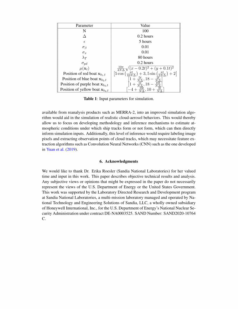
Parameter ValueN 100∆ 0.2 hoursε 5 hoursσβ 0.01σx 0.01λT 80 hoursσpd 0.2 hoursµ(xt)

10π4N∆

√(x− 0.2t)2 + (y + 0.1t)2

Position of red boat xb1,t[5 cos

(πt

10N∆

)+ 3, 5 sin

(πt

2N∆

)+ 2]

Position of blue boat xb2,t[1 + 5t

N∆ , 18− 2tN∆

]Position of purple boat xb3,t

[1 + 5t

N∆ , 18− 10tN∆

]Position of yellow boat xb4,t

[−4 + 10t

N∆ , 10 + 2tN∆

]Table 1: Input parameters for simulation.

available from reanalysis products such as MERRA-2, into an improved simulation algo-rithm would aid in the simulation of realistic cloud-aerosol behaviors. This would therebyallow us to focus on developing methodology and inference mechanisms to estimate at-mospheric conditions under which ship tracks form or not form, which can then directlyinform simulation inputs. Additionally, this level of inference would require labeling imagepixels and extracting observation points of cloud tracks, which may necessitate feature ex-traction algorithms such as Convolution Neural Networks (CNN) such as the one developedin Yuan et al. (2019).

6. Acknowledgments

We would like to thank Dr. Erika Roesler (Sandia National Laboratories) for her valuedtime and input in this work. This paper describes objective technical results and analysis.Any subjective views or opinions that might be expressed in the paper do not necessarilyrepresent the views of the U.S. Department of Energy or the United States Government.This work was supported by the Laboratory Directed Research and Development programat Sandia National Laboratories, a multi-mission laboratory managed and operated by Na-tional Technology and Engineering Solutions of Sandia, LLC, a wholly owned subsidiaryof Honeywell International, Inc., for the U.S. Department of Energy’s National Nuclear Se-curity Administration under contract DE-NA0003525. SAND Number: SAND2020-10764C.

References

Berner, A. H., C. S. Bretherton, and R. Wood (2015). Large eddy simulation of ship tracksin the collapsed marine boundary layer: a case study from the monterey area ship trackexperiment. Atmospheric Chemistry and Physics 15, 5851–5871.

Blossey, P. N., C. S. Bretherton, J. A. Thornton, and K. S. Virts (2018, August). Locallyenhanced aerosols over a shipping lane produce convective invigoration but weak overallindirect effects in cloud-resolving simulations. Geophysical Research Letters, 9305–9313.

Capaldo, K., J. J. Corbett, P. Kasibhatla, P. Fischbeck, and S. N. Pandis (1999). Effectsof ship emissions on sulphur cycling and radiative climate forcing over the ocean. Na-ture 400(6746), 743–746.

Carslaw, K. S., L. A. Lee, C. L. Reddington, K. J. Pringle, A. Rap, P. M. Forster, G. W.Mann, D. V. Spracklen, M. T. Woodhouse, L. A. Regayre, and J. R. Pierce (2013). Largecontribution of natural aerosols to uncertainty in indirect forcing. Nature 503, 67–80.

Conover, J. H. (1966). Anomalous cloud lines. Journal of Atmospheric Science 23, 778–785.

Council, N. R. (2015). Climate Intervention: Reflecting Sunlight to Cool Earth. Washing-ton, DC: The National Academies Press.

Eyring, V., I. S. A. Isaksen, T. Berntsen, W. J. Collins, J. J. Corbett, O. Endresen, R. G.Grainger, J. Moldanova, H. Schlager, and D. S. Stevenson (2010). Transport impacts onatmosphere and climate: Shipping. Atmospheric Environment 44(37), 4735–4771.

Gunnar, M., D. Shindell, and F. M. Bre on and W Collins and J Fuglestvedt and J Huang andD Koch and J F Lamarque and D Lee and B Mendoza and T Nakajima and A Robock andG Stephens and T Takemura and H Zhang (2013). Anthropogenic and natural radiativeforcing. In T. F. Stocker, D. Qin, G. K. Plattner, M. Tignor, S. K. Allen, J. Boschung,A. Nauels, Y. Xia, V. Bex, and P. M. Midgley (Eds.), Climate Change 2013: The PhysicalScience Basis. Contribution of Working Group I to the Fifth Assessment Report of theIntergovernmental Panel on Climate Change, Chapter 8. Cambridge, United Kingdomand New York, NY, USA: Cambridge University Press.

Latham, J. (1990). Control of global warming? Nature 347(6291), 339–340.

Possner, A., H. H. Wang, R. Wood, K. Caldeira, and T. P. Ackerman (2018). The efficacyof aerosol–cloud radiative perturbations from near-surface emissions in deep open-cellstratocumuli. Atmospheric Chemistry and Physics 18(23), 17475–17488.

Possner, A., H. Wang, R. Wood, and T. P. Ackerman (2018). The efficacy of aerosol-cloud radiative perturbations from near-surface emissions in deep open-cell stratocumuli.Atmospheric Chemistry and Physics 18, 17475–17488.

Riemer, N., M. West, R. Zaveri, and R. Easter (2008, 09). Simulating the evolution of sootmixing state with a particle-resolved aerosol model. Journal of Geophysical Research:Atmospheres 114, D09202.

Sofiev, M., V. Sofieva, T. Elperin, N. Kleeorin, I. Rogachevskii, and S. Zilitinkevich (2009,09). Turbulent diffusion and turbulent thermal diffusion of aerosols in stratified atmo-spheric flows. Journal of Geophysical Research: Atmospheres 114, D18209.

Twomey, S., H. B. Howell, and T. A. Wojciechowski (1966). Comments on “anomalouscloud lines”. Journal of Atmospheric Science 25, 333–334.

Wang, H., P. J. Rasch, and G. Feingold (2011). Manipulating marine stratocumulus cloudamount and albedo: a process-modelling study of aerosol-cloud-precipitation interac-tions in response to injection of cloud condensation nuclei. Atmospheric Chemistry andPhysics 11, 4237–4249.

Yuan, T., C. Wang, H. Song, S. Platnick, K. Meyer, and L. Oreopoulos (2019). Auto-matically finding ship tracks to enable large-scale analysis of aerosol-cloud interactions.Geophysical Research Letters 46(13), 7726–7733.