Embed Size (px)
Citation preview
ANNALS OF PHYSICS 137, 213-261 (1981)
Legendre Transforms and r-Particle Irreducibility in Quantum Field Theory: The Formal Power Series Framework*
ALAN COOPER,JOEL FELDMAN, AND LON ROSEN
Mathematics Department, University of British Columbia. Vancouver, British Columbia V6T 1 Y4. Canada
Received May 27, 1981
We study the higher Legendre transforms p”{A } of the generating functional G for connected Green’s functions in Euclidean boson field theories. To analyze P” (A } rigorously even when it does not make sense as an ordinary functional, we develop the framework of formal power series in A. For r = 1. 2 we isolate regularity conditions on G that ensure the existence of r(r) as a formal power series and we verify these conditions for the weakly coupled P(g), model. We also establish the improved regularity of the functional 0”’ obtained by subtracting from r”’ its trivial singular part.
I. INTRODUCTION
This paper, together with its companion paper (2; hereafter referred to as I], form the foundation for our series (3-51 devoted to the (higher) Legendre transforms Pr) (A ) of the generating functional G(J ) of connected Green’s functions in Euclidean quantum field theory. Legendre transforms have appeared in a wide variety of roles in both quantum lield theory and statistical mechanics in connection with symmetry breaking, computation of the effective potential, renormalization, definition of the coupling constant, etc. In this series we focus on the remarkable role played by F” in generating the r-irreducible vertex functions and a number of other field-theoretic objects with r-irreducibility properties in certain channels (such as Bethe-Salpeter kernels and r-irreducible expectations).
The higher Legendre transforms were introduced by De Dominicis and Martin ] 71 and further analyzed by Vasil’ev et al. [ 161. These authors established, in the context of perturbation theory, that for Y < 4 T”‘(A} essentially consists of the r-irreducible (amputated) graphs in G(J). One of the main contributions of our program is to formulate and prove these r-irreducibility results independently of (divergent) pertur- bation theory. In so doing we obtain model-independent proofs that, we believe, are much simpler and reveal more clearly the structure of P” than the nonrigorous perturbation theory arguments.
* Research partially supported by the Natural Sciences and Engineering Research Council of Canada.
213 0003.4916/81/140213119%05.00/0
Copyright C’ I98 I by Academic Press. Inc. All rights of reproduction in any form reserved

214 COOPER, FELDMAN, AND ROSEN
The key to unlocking the notion of r-irreducibility from perturbation theory is Spencer’s idea [ 141 of t-derivatives. Very briefly the idea is as follows (see I for a detailed explanation). Suppose we replace the free propagator or covariance C = (-d + rni)-’ of a Euclidean scalar boson theory by
c(t) = tc + (1 -t) c,, O<t<l, (1.1)
where C, = (-A,, + rni)-’ has Dirichlet B.C. on a smooth (d- I)-dimensional surface u c Rd that separates Rd into two regions. That is, we replace the Gaussian part &, of the measure defining the theory by the Gaussian measure d&,,. In this way all field-theoretic objects acquire a t-dependence; in particular, graphs in a perturbation expansion have a factor C(t)(x, y) > 0 (instead of C(x, y)) associated with a line joining the vertices x and y. At t = 0, C(O)(x, v) = CU(x, J’) vanishes if and only if x and y are separated by CI (we denote this by xay); on the other hand
W(x, y) = C(x, Y> - C,(x, v> > 0 (1.2)
for all x # y. It follows that a graph F(t) has r + 1 lines crossing o if and only if 3-(O) = a,.F(O) = . . . = a;.L?(O) = 0 but a;+ ’ Y(O) # 0. This observation allows us to define the r-irreducibility of a graph, or more generally of any field-theoretic object, in terms of the vanishing of certain of its t-derivatives at t = 0, &ith no reference to perturbation theory. (See Section II of I.)
Spencer’s idea by itself does not produce rigorous proofs of r-irreducibility. In I we presented proofs of the irreducibility properties of pi’ and p2’ that were formal in the sense that we did not establish that F”(t) and P)(t) existed, that they were regular in t (or in their other arguments), or that various formulas for &I’@’ made sense. For the case of the weakly coupled P(#)2 model (hereafter denoted EP(#)~) and for t = 1, Glimm and Jaffe [lo] have shown that T’*‘{A} exists as a genuine functional for suitable A and we have established the analogous result for r(*’ [61. But these proofs are highly technical and almost surely do not extend to r > 2 or to models involving fermions. The main purpose of this paper is to develop a general framework which does not entail the existence of p” (A} as a genuine functional but which permits one to draw rigorous conclusions about the generalized vertex functions SiPr’{O} on the basis of arguments like those of I. This is the framework of formal power series (fps).
Before describing what we mean by fps, we recall the (formal) definitions of PI’ and p2’ from I. Let (.) denote the (Euclidean) expectation defining a scalar boson field theory (e.g., an EP(#)~ theory). If JE Cr(iRd) and L E C,“(lRd x Rd)sym., let
G”‘{J} = In Z”‘(J) = ln(em.J) (1.3)
and
G(*){J 3 L} = In &*){J} = ln(e”J+02.L >9 (1.4)

LEGENDRE TRANSFORMS 215
where repeated (but possibly suppressed) variables are integrated over; e.g., #” . L = j:r‘ Q(x) o(u) L(x, 4’) dx dy. Define
dG(” A iJl(x) = &J(x) iJ1 - A,(x)9
where
(1.5)
(1.6)
If the functional A(J) is invertible with inverse J(A} then we define the first Legendre transform by
I-“‘{A} = G”“(J(A}} - G;“(J(A )} . J(A}.
where G:” . J = i (6G”‘/U(x)) J(x) dx. We also define
@“‘(A} = P)(A) + ~Ac’A.
From Definition (1.7) we easily obtain the dual relation to (1.5)
J= -,‘,”
and the Jacobian relation
(1.7)
(1.8)
(1.9)
r’,‘, zz -JA = -I&-’ = -(G;;‘)-‘. (1.10)
To define the second Legendre transform we set
(1.1 la)
and &3’2’
B(J. L I(-GY) = 6J(xj sJ(y) (J, L \ - B,(x, Y)
iiG’*’ (1.1 lb)
= 6L(x,y) iJ,LJ - (A(x) +A,(x))(A(Y) +A,(y)) - B,(x,y).
where
B,(x, y) = &3t2,
&J(x) ~J(Y) (05 01 = (4(x); $0)). (1.12)
where the semicolon indicates truncation. If the map J = (J, L) --) A = (A, B) given by (1.11) is invertible with inverse J = J{ A}, then we define
p*‘(A,B} = G’*‘{J, L) - G;“(J, L) . J- GI*‘(J, L} . L (1.13)

216
and
COOPER, FELDMAN, AND ROSEN
@(“{A, B} = I’(“{4 B} + $lC-‘A - j In det,(l + B; “‘BB;“‘), (1.14)
where In det,( 1 + H) = Tr(ln( 1 + H) - H). The relations dual to (1.11) are obtained by differentiating (1.13):
J = -T(‘) + 2I’f) . (A + A,), A L = -rf’. (1.15)
(In Sections III and IV we shall modify Definitions (1.7) and (1.13) by physically Wick-ordering the source terms. The resulting transform r(r)*w makes more direct mathematical sense although formally Pr),“’ = P”‘; see Theorem III. 1 and Lemma IV.2.)
If we introduce a t-dependence into the model as in (1.1) then r(r) acquires a t- dependence in the obvious way; we indicate this dependence by writing p”(A; t) and r”‘{A, B; t}. Note that we regard A and t as independent arguments of r’” (and similarly for p*)). Now to show for example that r(l) is l-irreducible we must prove that for r’ = 0, 1 (see I)
.(1.16)
if xay (i.e., if the surface 0 separates x and y). The virtues of the criterion (1.16) are (i) it is nonperturbative, (ii) by using the generating functional fi’) we handle all the vertex functions r(ni) at once, and (iii) t-derivatives are easy to compute. In particular, we have from (1.7), taking into account the fact that J = J&4; t},
fi” = (#” + G:” . j) - (G;” . j + (a$:“) . J)
=@‘-A 0
. J (by (1.5)) (1.17)
= @I’ + A . PI’ 0 A (by (l-9)).
Here G(‘), the t-derivative of G(‘) with J fixed, is readily computed to be (see (3.13) of I)
G(1) = -@I : [G;;’ + G;“G:“];, (1.18)
where (3-i = -C-‘&-i, C-’ : F = sl C’-‘(x, y) F(x, y) dx a”, and [H]$ = H{J} - H{O}. For r = 2 we have
~2~=-~iC-1:(B+A2+2AAo)+I-A~o+T~~o. (1.19)
By means of formulas like (1.17)-(1.19) we can reduce the question of the r- irreducibility of P’) to questions about the O-irreducibility (E connectedness) of objects not involving t-derivatives.
Do the above definitions and calculations make mathematical sense? If we regard Ztr) and G(‘) as genuine functionals we must first face the question of their existence

LEGENDRE TRANSFORMS 217
on a suitable space of test functions. Then we must face perhaps the most difficult question involved in the above definitions, namely the invertibility of the functional A{J/. For r > 2 the situation seems hopeless since, for example, for a free theory ZC3’ = (e”“‘“J) diverges. However, since our primary interest lies in the generalized vertex functions (= moments) of rtr) for arbitrary I, we can avoid most of these difficult analytic questions by working in the context of formal power series. The fps calculus retains the computational and conceptual advantages provided by the generator
F(f} = \g &J” - n! n=O
(1.201
of a family of functionals (F,}, even when the series (1.20) diverges. The idea is simply to interpret the symbol F as the sequence of coefficients {F,} and to define operations F--t F’ by the corresponding mappings of coefficients {F,} -+ (Fk \. For most standard operations, Fk is given by afinite expression in the F,‘s. Hence we can avoid questions about convergence of infinite series while still drawing conclusions about the F,‘s with no sacrifice of mathematical rigour. (We emphasize that the series considered here are not the perturbation theory series.) Of course, in many situations (1.20) will converge to define a genuine functional. Naturally, we shall make our definitions in such a way as to ensure the consistency of the fps and functional points of view whenever they both make sense.
For example, as fps, (we suppress the superscript 1 in (1.3))
Z{J} = (e”‘“) = c $ S, . .I”, “Zt) .
will just represent the sequence (S,} of Schwinger functions, and the operation Z(J} + G{J\ = In Z{J} will be interpreted as the mapping IS, I+ (G, 1. where G, = 0, G,=S,, G2=S2-S:,etc.
As another example, to define r”’ as a fps we just have to define all the Pfl”‘s. Ultimately the fps interpretation of the definition (1.7) of r(” reduces to the familiar tree-graljh expansion (see Section VI of I) which represents each r’,” as a finite expression involving G,‘s with m < n and the inverse operator G; ‘; e.g..
l-(41) = (G; ‘)” G, - 3(G, ‘)’ G, G, ‘G,(G; ‘)I.
In this paper we develop the framework of formal power series as a mathematical basis for the definitions and analysis of P1’ and p2’ in I as well as for our further analysis of r(r) (r > 1) in [3-51. The point is that all the operations involving pr) can be rigorously interpreted in the fps context under a few reasonable assumptions on the S,,‘s (such as the existence of G;‘). These operations are of the following types:
(1) Linear operations such as sums, scalar multiples, functional derivatives (e.g., S,G{J}), parameter derivatives (e.g., a,G), and composition with a linear operator;

218 COOPER, FELDMAN, AND ROSEN
(2) Products and quotients, including scalar products (e.g., G, . J in (1.7)), operator products, and operator inverses (e.g., G,;’ in (1.10));
(3) Compositions (e.g., G{J{A )}, G(J} = In Z{J)) including the construction of composition inverses (such as J{A}).
In Section II we develop a general fps calculus that incorporates all of these operations. In Section III we apply this calculus to the construction of F’) (as a fps) and to a justification of the computations (like (1.17) and (1.18)) that we used in I to establish the l-irreducibility of r (I) Section IV is devoted to the corresponding . analysis for p ‘) We have formulated the theorems of Sections III and IV along . general lines in terms of hypotheses about G (I) pr), A{J} etc. that we believe to be , reasonable for a wide range of models.
As support for this belief we have verified these hypotheses for the EP(~)~ model (see Theorems V. 1, V.5, and V.8). Since Theorem V. 1 holds for all r > 1 we have deferred its actual proof to our paper on pr) [3]. Instead, the bulk of Sections V and VI is concerned with a special feature of the cases r = 1 and 2, namely the improved regularity of the functionals @ (r). The definitions (1.8) and (1.13) of @(‘) have been chosen so as to remove all C-l’s from Fr) (in perturbation theory). As a rigorous expression of this, we find that for the EP(@)~ model @“‘(A) can be extended to test functions A that are required only to have certain L* regularity properties with no additional differentiability requirements (this is the content of Theorems V.5 and V.8). In determining the appropriate space for A, we have found the amalgam-Lp or Birman-Solomjak Zp(L9) spaces [ 1, 131 extremely useful. The virtue of these spaces is that one can decouple the local regularity of the test functions from their global regularity (i.e., decay at co). In Lemmas V.3 and V.7 we establish estimates for integral operators on 1*(L9) that may be of independent interest.
Thus the basic distinction between pr’ and @@) (as far as their regularity is concerned) is that the functions in the domain of T(r) must be in the form domain of C(t)-’ and in particular must vanish on u at t = 0, whereas there are no differen- tiability or boundary conditions on the functions in the domain of @(“. Consequently, we say that @(I’ is “r-cluster-irreducible in the extended sense” (see I). On the other hand the difference $4C-‘A between pl’ and Q(l) is not l-irreducible in the extended sense; but upon restricting A to be in L/f’, = CF(lR’\u) it is r-irreducible (for all r!) since
c-I( = 0 if A E<dz (1.21)
(see (3.17) of I). Hence r”’ is l-irreducible. The identity (1.21) also plays an important role in our irreducibility proofs for pr’ when r > 1 [2,4].
II. THE POWER SERIES FORMALISM
We now make precise our notion of formal power series (fps), define the operations on them that are of interest in our analysis of the Legendre transforms, and establish some basic properties.
LEGENDRE TRANSFORMS 219
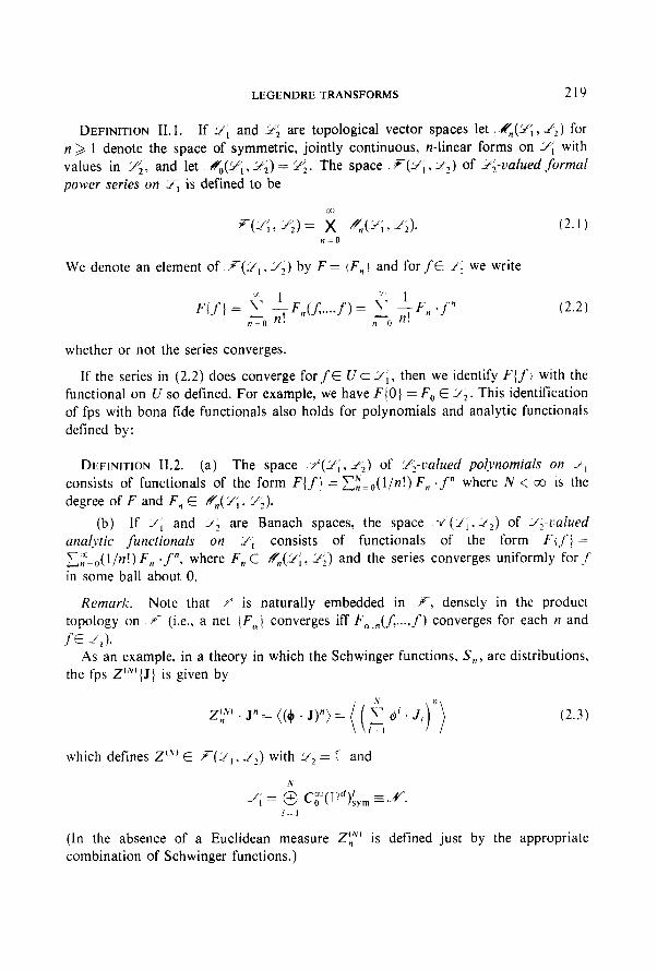
DEFINITION II. 1. If Y{ and 2; are topological vector spaces let L.4n(U;, I;) for n > 1 denote the space of symmetric, jointly continuous, n-linear forms on 56; with values in Yz, and let &(Y,, Pz) = S$. The space ,8(li;, 2;) of Pi-valued formal power series on Y; is defined to be
qIi;, q = ; qLcL;/; ) 2;). (2.1) ?7=0
We denote an element of. F(-r/, .2,) by F = (F,) and for fe I, we write
(2.2)
whether or not the series converges.
If the series in (2.2) does converge for f E U c 2;, then we identify F( f } with the functional on U so defined. For example, we have F(0) = F, E Yi,. This identification of fps with bona fide functionals also holds for polynomials and analytic functionals defined by:
DEFINITION 11.2. (a) The space .O(Y;, L.$) of Ii-valued polynomials on I, consists of functionals of the form F( f } = Ct=,( l/n!) F, . f n where N < co is the degree of F and F, E Yn’a,(~;, Yz).
(b) If 1, and 1; are Banach spaces, the space ,v’(I,, I(,) of ;/2-t~alued analytic functionals on 2, consists of functionals of the form F{f‘} = ~~Lo(l/n!) F, .f", where F, E fln(Yi, rC;> and the series converges uniformly for f in some ball about 0.
Remark. Note that .Y is naturally embedded in ,5-, densely in the product topology on ?- (i.e., a net (FQ) converges iff F,,,(f,..., f) converges for each n and SE-J,)*
As an example, in a theory in which the Schwinger functions, S,. are distributions. the fps Z’“’ (J } is given by
Zl;“’ . J” = ((9 . J)“) = ((+i.Ji)“)
which defines Z” E. ii(l/, , 12) with I/, = C and
(In the absence of a Euclidean measure ZL”’ is defined just by the appropriate combination of Schwinger functions.)

220 COOPER, FELDMAN, AND ROSEN
Linear Operations and Derivatives
Definition II. 1 automatically provides X(g, Yz) with a linear structure (i.e., (aF + bG), = aF,, + bG,), and natural definitions of continuity and differentiability with respect to a parameter and of composition with a linear operator. For example, if Ti is a continuous linear operator on g then T2 o F o T,{f} = T,(F{T,f}) is defined as a fps in <FT(Pi;, Yz) by (T, 0 F 0 T,), . f n = T,(F, . (T,f)“).
If FE S(iq, jti2), its (Gateaux) functional derivative is defined by
This definition extends by continuity to give:
DEFINITION 11.3. If FE LF(P1, Yz) then the fps functional derivative, SF/& E S,F E F,, of F is defined as a fps in ;T(Y, , Ai(ik,, PI)) by
( 1 5 ” Cfo,...,fo):f~Fn+,dfo,...,fo,f) (2.4)
for f, and f in Y1. In particular, if FE R(Pr, C) then SF/Sf E X(9,, YT). Similarly, taking m derivatives maps ;“(P,, Pz) into Y(ip, , Am(q) PI)) according to
(sf”F),f~:f”-F,,,f;ff”. (2.5)
With this definition it is easy to see that F, = 6fmF{O} so that for the example (2.3)
qzZ’N’{O} = s,,.
Products
Let n be a jointly continuous bilinear map from 9~‘) x 9’:‘) to 9i3’. Many of the products that occur in our paper are of this type such as
(a) Yi’) = 9(.K1,.K1), 9i” = 9(&, S3) and Pi3’ = ,9(S”,,.S3) with rc = operator product, where SK,, .&, S3 are Banach spaces and &@‘~, Cq) = bounded linear maps from & to .Kj (with norm topology).
(b) 9;” is a Frechet space, Py) = Pi*‘*, 9;“’ = C and rc is the functional pairing 4fi9f2) =fdf2) = (f, ,f2).
(c) Y’$l) = C and rr = multiplication by scalars.
For any such n and any 4” we can define a related jointly continuous bilinear map from Y(gl, 9;“) X X(9,, Pi*‘) to XT(g) 9i3’).
DEFINITION 11.4. The fps product
x(F(l), F’*’ ){f 1 = 4FYf 1, F’*‘{f I)

LEGENDRE TRANSFORMS 221
is defined by
For example, let cr be a separating surface for IRd (as described in Section I) and let P, be the linear maps on
4= 6 ca(~“\dl,,nl I=0
defined by (P, J),(x, ,..., x,) = ni= , x+(xi) J,(x, ,..., x,), where x+ is the characteristic function of the + side of 0, and similarly for P_. Then using (2.5) with F”’ = z’“’ 0 P, , F”’ = Z’“’ 0 P- E .X(X0, C), and rr being ordinary multiplication in cc. we have
Z’,“(P, J} Z’,“{P_J) = c -$ 2 (; j ((4. P+J)“)((+. P J)” “). fl=O m-0
In a local model with C replaced by C(t) as described in Section I we have by virtue of the locality of the interaction that, at t = 0,
((4 + P, J)m(+ . P-J>“-“) = ((4 + P, J)m)((4 * P-J)“-“). (2.6a)
Hence, for J E XV we have
(4 . P, J)m(+ . P-J)‘-“’ (2.6b)
= Z’N’{P+ J) Z’N’(P- J).
LEMMA II.5 (Product rule for derivatives). Whenever the right-hand sides make sense. we have
(b) d
zW”){f; t), F’*‘(f; t})
(2.7a)
= 71 F’1’l.f; f), p/s; t)) + 7r ($F(“(f: q,pQ-; t)) (2.7b)

222 COOPER,FELDMAN,AND ROSEN
ProoJ These formulas extend by continuity from Pi) in 9 to all of Rci’. (Alter- natively, the same straightforward computation that provides the proof for .P also works directly for KCi).) 1
LEMMA II.6 (Multiplicative inverses). Let 92=2S(Sl,S2) and YP;‘= 3’(X,, X,). If F E ;T(Yl, 4k;) with F, invertible, then there exists a unique element F-’ of Y(q) 5/p; ‘) with F-IF = Z, and FF-’ = I,, where Ij is the identity operator on Sj. Furthermore, we can compute derivatives for F-’ by
and
dF-l=-~-l?J~-l dt
(2.8a)
(2.8b)
and repeated derivatives by iteration so long as F itself is suf$ciently dlflerentiable.
Proof: A left inverse FL if it exists satisfies FLF = I, which means by Definition II.4 that FtF, = I, and for n > 1, C~=,($)(FL), F+,,, = 0. These equations can be solved recursively for the (FL),,% starting with (FL), = F;’ and obtaining after n steps a finite expansion for (FL), in terms of F;’ and F, with m < n. A right inverse can be constructed similarly and equality and uniqueness follow by the usual group theory argument. The derivative formulae are straightforward consequences of the product rule. m
Composition of Formal Power Series
Imials’ F E 9(g, L$), G E 9(Pz, P3) of degree N and M respectively For polyna we have
G{F{f
In general, for each n the number of terms in the sum over m depends on G, but if F, = 0 then ki = 0 is excluded and so EYE, ki = n forces m & n. Thus:
DEFINITION 11.7. If F, = 0 we define the fps composition (G 0 F){f } = G{F(f }} by
(G~QU”)= 5 1 i: m=O Ifl.
(k .;.k, G,(F,, fkl,..., Fk,f km)m (2.9) k,,...,k,=O 1

LEGENDRETRANSFORMS 223
This defines a (separately) continuous map from {F E .F(ik; , ik;) 1 F, = 0) X
ii( li; , Y3) to P-(2; ,2g. As an example take F =Z”“‘- 1 and G(x) = ln( 1 + x) to define G’“‘(J 1 =
In Z’“‘{J) as a fps on X whenever the S,,‘S are distributions. Now the identity
is immediate if the Z,‘s are polynomials and extends by continuity to the case of general formal power series. Combined with (2.6b) this proves the connectedness of G . IA).
LEMMA 11.8. If the 27,‘s are distributions which cluster according to (2.6a). then G”“(J) exists (in “(-K. C)) and is connected.
LEMMA 11.9 (Chain Rule). Let FE .ir(Y,, 2;) and G E, ~T(Y~, 2’;) with F,, = 0. Then \ce hare
(a) (2.10a)
(b) If F(f; t) and G(f; t) each depend differentiably on a parameter t, then
r
~G{FIf;li;r/=~iFif:t}:r}+~{F(f;I);ti~(.f:t}. (2. lob)
Remark. In (2.10a), 6G/6F E .F(P;, e(Y;, -;/;)I, (6G/i?F){F} E.i’2,, e(Lr,, 23)), 6F/6f E.7(Yik;,.<(Y,, P$), and (2.10a) is an identity in F(bi;. <(y;,I(;)). The product on the right is always well-defined by (2.5). (However, if the 2; are general topological vector spaces, it might fail to be jointly continuous.)
ProoJ: By polynomial approximation (using truncations of G and F). 8
As a simple application of this Lemma we have
so G, = S, and
GJJ=$ ;ZJ =;Z,,-$zJz, ( 1
so Gz=Sz-S,S,. etc.
224 COOPER, FELDMAN, AND ROSEN
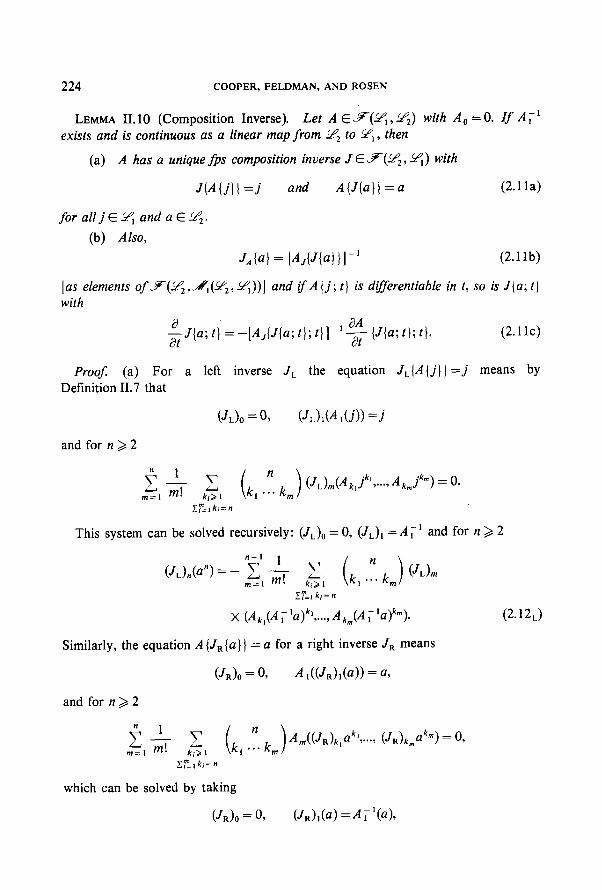
LEMMA II. 10 (Composition Inverse). Let A E.F(YI,Yz) with A,=O. If A;’ exists and is continuous as a linear map from 9.. to 4”,, then
(a) A has a unique fps composition inverse J E X(5$, 9,) with
JVLO) =j and A{J{a}i=a (2.1 la)
foralljeg, andaE9,.
(b) Also,
J&J = kb{JbWI-’ (2.1 lb)
[us elements of F(Yz,&(Yz, -!&:>)I and ifA{j; t} is differentiable in t, so is J{a; t} with
$ J{a; t} = -[A,(J{a; t}; t}]-‘g (J{a; t}; t}. (2.1 lc)
Proof: (a) For a left inverse J, the equation J,{A{ j}} = j means by Definition II.7 that
(Jdo = 0, (JJ,@ ,(A> =j
and for n > 2
i 4 2 m=I m. ki> 1
(k *Ye k ) (JL)m(Ak,jk’,...,Ak,jk,) =a 1 m
Xy=lki=n
This system can be solved recursively: (JL),, = 0, (Jt), = A;’ and for n > 2
(Jd,@“) = - nfl 4 c m=I m. ki>l
(k .T. k, (Jdm 1 )
-YE, ki= n
X (Ak,(A; ‘~2)~‘,..., A k,(A ; ‘a)km). (2.12,)
Similarly, the equation A{J,{a}} = a for a right inverse JR means
(Jdo = 0, A ,((Jd,(a)) = ~3
and for n > 2
f -$ c rn=I * ki> 1
( * )A,((&)k ak1y...9 tJR)k,~km)=Oy k, ... k, I
zbl ki=n
which can be solved by taking
(J& = 0, (J,d,W=A;‘@),
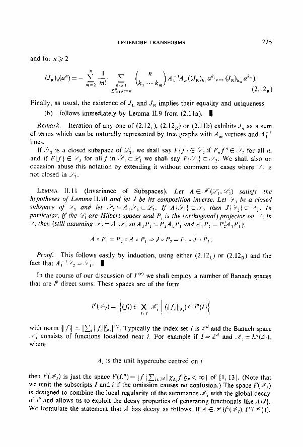
LEGENDRE TRANSFORMS 225
and for n > 2
(J,),(d) = - =+ J- - m! ml=2
(kl .“. k,) oMJdk, dl?...> (JJkP).
‘b, ki=n (2.12,)
Finally, as usual, the existence of J, and J, implies their equality and uniqueness.
(b) follows immediately by Lemma II.9 from (2.1 la). m
Remark. Iteration of any one of (2.12,), (2.12,) or (2.1 lb) exhibits J, as a sum of terms which can be naturally represented by tree graphs with A, vertices and A ; I lines.
If iz is a closed subspace of Yi, we shall say F(f} E ,i*, if F, f n E .Ui for all n. and if F( f } E iz for all f in .Y, c 9, we shall say F{ <‘?;I c ,Yz. We shall also on occasion abuse this notation by extending it without comment to cases where /: is not closed in Ye.
LEMMA 11.11 (Invariance of Subspaces). Let A E.iT(lk,, 2$) satis~~~ the hypotheses of Lemma 11.10 and let J be its composition inverse. Let ,i, be a closed subspace of I(, and let .;C2~Al..?,cit;. If A{,~,}c,/~ then J(i,}c.f,. In particular, if the 3 are Hilbert spaces and Pi is the (orthogonal) projector on fi in 2, then (still assuming .ii = A,. 7; so A, P, = P,A, P, and A, Pf = PtA , Pf).
Proof. This follows easily by induction, using either (2.12,) or (2.12,) and the fact that A;‘,>? =.‘i,. 1
In the course of our discussion of P we shall employ a number of Banach spaces that are P’ direct sums. These spaces are of the form
lP(,PI) = i (1;:) E x .q iEI
(Il./J $;) E P(Z) j
with norm i]lf]]l = [Ci ]]fi]]gi]““. Typically the index set Z is Id and the Banach space ‘1 consists of functions localized near i. For example if I = Zd and Si = Lq(di). where
A, is the unit hypercube centred on i
then fp(&) is just the space Ip(Lq) = {f / CisPd ]]xAif]]f4 < co) of [ 1, 131. (Note that we omit the subscripts Z and i if the omission causes no confusion.) The space /“(Xi) is designed to combine the local regularity of the summands 4 with the global decay of 1’ and allows us to exploit the decay properties of generating functionals like A(J). We formulate the statement that A has decay as follows. If A E, T(I’(,$i), [“( C;)),

226 COOPER, FELDMAN, AND ROSEN
we let P, (resp. Pi) denote the projection onto the summand 5, (resp. Xi) in Ii (resp. I”(%:)). For each 1 E 1’, let P, = P,l @ .. . @ Pi,. Introduce the norms
pi,,, = IIP$ 0 A, 0 P,J(
of the n-linear forms
Then
P;,oA,oP,:S4j,x . ..x.Y&.+%-;,.
DEFINITION II. 12. We say A E F(ll(XI), l”(Xj)) has decay if
suP C PiI. < O” ICI” i’E,T
Vn > 1
and we say A is invertible with decay if, in addition,
A{O} = 0 (2.13b) and
supc IIPiA;‘P;,I( < co. (2.13c) i ’ i
Remarks. (1) While a priori A E sT(ll(Z1), I”O(X;)) Condition (2.13a) ensures that pi,,, is the kernel of a bounded operator from 1’(Y) to l’(1) and hence that A EST(I’(S~), 1’(X;)). The A;’ of (2.13~) refers to the latter, i.e., to A, E&(ll(-%), l’@?)).
(2) Conditions (2.13b,c) have been introduced so the composition .inverse J{A} automatically has decay if A{J} does. The existence of J{A } forces A(0) = 0 and A;’ to exist and the decay of A;’ is essential in:
LEMMA II.13 (Preservation of decay). (a) IfA{J} E F(l’(SI), l’(X;)) is inuer- tible with decay then its composition inverse J{A } is invertible with decay.
(b) ZfZ{J} EST(I’(X,), C), Z(0) # 0 and L’,(J) has decay then (S/SJ) In Z{J} has decay.
ProoJ: (a) We control li+tS = I(Pi o J, o P;,II by induction on n. For n = 1 the desired estimate is just (2.13~) since J, = A; ‘. For n > 1 (2.12,) expresses J,, as a finite linear combination of terms of the form J,,, o (Ak, @ +. . @ Ak,) 0 (A ;‘O”) with l<m<n.But
lIPi 0 J,,, 0 (Ak, @ ..a @ Ak,) 0 (A;‘)‘” 0 P;,)I

LEGENDRETRANSFORMS 227
Each factor here obeys (2.13a). Hence repeated use of
sup c p P& k) &A) < (yp 2 P(& k)) (“7~ c c(U)) j i k I k
yields the desired estimates.
(b) Denote (S/SJ) In Z{J) by AS{J). Then
A;. = @(z,z-‘) = 5 WI=0 ( )
; [ZJmil(Z-‘)J”-m]sym
SO
z-‘(J) 12=i\ir
But
since Z- ’ E X(1’(&), c) and
by the decay of Z,. 1
III. CONSTRUCTION OF P1)
We now consider the construction of T”‘{A; t) in the fps framework we have just developed. If the Schwinger functions (S, j are distributions then we know G(J; t 1 E , T(, I ; C) and A {J; t} = G,{J; t) E .F(J’-,-k”*), where -4’” = Cp(lRd). The crucial step in the construction of r (we will suppress the superscript (1) for a while) is the inversion of the map A {J}. According to Lemma II. 10, A will be invertible as a map from some vector space ik; to another PI provided both that A,{O) = G,,{O} = G, is continuously invertible as a map from Pi to Pz and that A {Y, ) c Pz. A natural way to ensure this is to require that G, be (strictly) positive, thereby defining a norm Ilfll,$ = G,dj’,,f), and to require that for n > 2, G, = G,,{O} extend continuously to ;;z”G? (the completion of ,4‘ in 11. II,,). Then by Lemma II. 10 A {.I} E F(o?&~), GF&,~,)
595/137/2-2
228 COOPER, FELDMAN, AND ROSEN
and J{A I E ~W&, .+&)). We remark that if the Schwinger functions are given by a measure then Gtdf,& t) = (Id(J) - (#(j))tl’), is always positive; if t = 1 G, is always strictly positive by the Kallen-Lehmann spectral representation; if t = 1 and the theory is canonical and has a mass gap then ]]f]lG, is equivalent to ]]f]l, = (f. C!!)V2. Hence another way to ensure the invertibility of A {J, f} is to require (as suggested by perturbation theory and verified for EP(#)~ in [lo] that for all n > 2 G,(t) E ~$(.9’~, C), where
(3.1)
and that G,, viewed as an operator from B! to 9, , * have a continuous inverse. We do not expect G, EJr(91, C) in general, for in a covariant theory G, is a constant. Hence in general G{J, t) 65 Sr(st, C). This is at worst a nuisance since under the above hypotheses
G@‘{J; t) G In Zw{J; t} 2 ln(ei’)l z ln(e’m-cB’r’)l
will be in .Y(5Yl, C) and
(3.2)
fW{A } = GW(J(A )) - G,W{J{A ) } - J(A ]
will be in sT(9:, C). Formally
(3.3)
Z+‘{A} E G{J{A}} -G, -J{A} - [G,{J{A}} - G,] - J{A} (3.4)
= Z-{A}.
Alternatively suppose the theory has decay in the sense that for all n > 2 there exist constants m, > 0, c, with
I G,df, ,...,f,)l < c,, C IIxA, C(t)“*f, IIt2 ifJ e-mnd(A’,Ar) IIxA, C(t)“‘f;:llt2 Ai (3-5)
I(f,, G;‘f,)l < ~2 g lI~A,C(~)-~*f,ll~~ e-m2d(A1*A2) IIxA,C(~)-“*~IIL~~
(Such decay is often a consequence of the connectedness of G.) Then A{J; t} is inver- tible with decay (see Definition 11.12) as a map from r’(9t) to I”(gf), where
(where the subscript I = Zd has been suppressed). Furthermore the preservation of decay lemma (Lemma 11.13) implies that A{J; t} E Y(f’(gt), 1’(9:)) and J{A; t} E F(P(9’T), t’(.9J). As a result we can define G, . J and hence G(J(A} } provided G, E l”(2’;).
The net conclusion of this discussion is

LEGENDRETRANSFORMS 229
(3.7)
(3.8)
THEOREM III.1 (Existence of the first Legendre transform).
(a> rS (i) ZW(J; t} E.F(,$(, C),
and (ii) Gz: ,Y?~--+, ST’: has a continuous inverse
then P’(A } E .F(S~f, C).
(b) If (i) A (.I; t) E .F(l’(.St), /‘(.-ST)) is invertible with decay,
(ii) G, E I”(.9:),
then T{A ] E, Y(l’(.ijp~), C) and T(A ) = TW{A } on l’(.S:) c .&F.
Remark. The hypotheses of this and all subsequent propositions are true for FP(~)* and are verified either in Section V or in [3].
The formalism also admits t-derivatives, and in fact under suitable restrictions on the model and on the variable A, every term in (1.17) and (1.18) makes sense. Now in a free theory G{J; t) = JCJ =JC(l)J - JC(O)J. Since C(0) < C(l), we need J E 9,~ ,dO for the existence of JCJ. It is thus natural to assume (as suggested by perturbation theory) that GW{J; t} is differentiable in .F(.9’, , @). To make sense of 6” {J(A)} and the other terms occurring in (1.17) and (1.18) we need to restrict the allowed values of A and we need G, sufficiently regular to ensure that for these values J(A } E 8,.
I-EMMA III.2 (Differentiability in t of r(l)).
(a) If (i) K(J; t) = C(t)-’ A (J, t} E X(9,, ~8,) and is dtfirentiable in t
and (ii) C(t)-’ G,: ,,SY, + .5?, has a bounded inverse,
then G”‘{J; t) E.F(-~, , C) and P’{A; t) E.T(L@, C) are d@rentiabfe in t and for A E. I;
Z+‘(A 1 = G”{J{A }}. (3.9)
tb) If (i) x(J; t} = C(t))’ A(J, t} E X(Z’(L~~), Z,(.g,)) is invertible with decay and
differentiable in t
and
then G(J; t) E .F(t’(S?,), @) and T{A; t} EF(t’(LF’,*), C ) are dz@rentiable in t and for A E. f,
j‘{A) &(J(A}) -A, .J(A}. (3.10)
230 COOPER,FELDMAN,AND ROSEN
Proof. (a) Since C(t) is differentiable in Ji(AY,, sT>, hypothesis (i) implies that GT(J; t} = C(t) A(J; t} is differentiable in Sr(.?8,, AI’:) and hence that GW{J; t) is differentiable in sT(AYi, C). Let .@I; t} denote the fps inverse map to A{J, t} so that for A E Jy, c SF
J{A;t}=J{c(t)-‘A;t}E9,.
Our proof of the differentiability of Tw is now based on the observation (Lemma V.2) that, when A E Jv,, C(t)-‘A is independent of t. Thus, when A E X0,,
I++‘{A; t) = GW{J{C(t)-‘A; t}; t) -A . J{C(t)-‘A; t}
= GW{J{C(I)-‘A; t}; t) -A .J{C(l)-‘A; t}.
By (i) and (ii) and Lemmas 11.9, II.10 this is differentiable in t, and so (by cancellation of the GyJ terms)
I+‘{A} =@+‘{J{C(l)-‘A}} = @“{I{A}}.
Now @‘{J{C(l)-‘A}} E ST(.%‘T, C) and Tw E R(A?$, c) (by Theorem 111.1). Therefore, approximating A E S,* c AZ?: by AZ E -flq and appealing to the uniformity in t of the convergence of fW(A,} = G”{J{C(l)-’ A,}} we find that TW{A} is actually differentiable in t for A E St. (But (3.9) need not be valid if A 6S Jz.)
(b) By (a) and Theorem III.lb, T(A) is differentiable on r’(AI’F) n S,* 3 1’(9,*) and when A EJY^,, f{A} = 6”{J{A}}. But, for such A our hypotheses ensure that J{A} =J{C(l)-‘A} E Z’(9,) and A,,, A, E P(JYf) = [1’(S,)]* so that Gw{J} = G{J} - A,,J, establishing (3.10). 1
We are now in a position to establish
THEOREM III.3 (l-Irreducibility of PI)). If in addition to the hypotheses of Lemma 111.2b,
(i) C-‘: G$I$ E jTQ’(AYi), c), C-‘A, E I”“(91), A, E I”(.9’T);
(ii) G”{5; t} = - iC-‘: [GEli + G,WG,W + 2A,G,W] -A,,&
then F1) is 1-I.
(3.11)
Remurk. We also, of course, assume that GW, C-‘GE and A,c’-‘G, are all con- nected.
Proof For A E -Kv the hypothesis (i) of Lemma 111.2b tells us that J(A) E l’(.JS1) and so for such A, we see by (3.11) and the arguments of Section III of I that Iy‘j = 0 at t = 0. 1
+-
Finally, the extended irreducibility of @ (‘) follows as in I so long as & E Y(Y, C) for some space 4p with M ~2: c Y. For EP(#)~ we establish this additional continuity in Theorem V.5.
LEGENDRETRANSFORMS 231
IV. CONSTRUCTION OF 11')
For the case of r<*), the linear term in G’*’ is again less regular than the higher order terms. In fact, the presence of terms such as Tr(CL) in the paturbation expansion for Gt2’{J} suggests that in order to define G”‘{J} we need [(Cl” @ C”*)L](x, x) E L1(Rd). On the other hand, the perturbation expansion for L {A )(x1, x,) includes terms with a factor 6(x, - x2) and these preclude [(CL” @ C”‘)L](x, x) E L’(Wd). Thus we do not expect to be able to make sense of the individual terms in the definition (1.13) of r(‘) (regardless of what regularity we impose on A and B).
We must therefore take advantage of the fact that the terms linear in J in (1.13) cancel. One way to do this is to interpret (1.13) to mean p”{A} =F(J(A)} with F defined by continuous extension of
F(J} = G{J} -J . G,(J} (4.1)
from J E CAr. However, we prefer to reexpress r(2) in such a way that the offending terms do not appear. For the case of Pi) we did this by working with GW(J} = G(J} - G,J. For p2) we find it convenient to go a bit further than just dropping the linear terms in Gc2’ and to work with “physically Wick-ordered” sources. That is, we let
where (5 = # - (4) and
$2; = i’ - ($2)
= 4’ - W4) - (4’) + w2. (4.2)
We can express GW in terms of G by
@“V, LI = G{J - 2L(#), L 1 -J(4) - L((ti2) - ‘W2)
=G{W’J\-A,&(II,,-A;)L (4.3a)
where WJ=(J-2LA,,L). (4.3b)
Hence G@‘(J, L} is defined at least for J EN if the S,,‘s are distributions, and is connected if (2.6) holds.
Actually, this approach is a bit of an insult to GW as it is really more regular than G (at least in the context of perturbation theory or such specific models as EP(#)~). In fact. for EP(#)~ we have [3]
(4.4a)
232
i.e.,
COOPER,FELDMAN,AND ROSEN
Z”{J} E (eJ’iK) EX(gt, C), (4.4b)
where (as in (4.14)) ]]f]]$ =fi C(t)fi +f;, C(t)@&. (For more singular models-eg., &-perturbation theory suggests that (4.4) fails, so that .9’t is not adequate for the sources in GW.)
We now let
and
AW{J}=G,W{J}=G,(WJ}-A,=A{KJ} (4.5a)
BW{J} = G;(J} - Gz(O} = G,w{J) - GJ”{J}*
=G,{W?}-G,,{O}=B{WJ}.
According to Lemma II. 10, the map J + Aw{J} will be invertible if
(4.5b)
is continuously invertible as a map from some q to P2 with AW(Pl} c g2. As in the case of pl) this will be so if MW is strictly positive and if GW(J} extends continuously to all of ZMw = (,v)‘l*‘1”‘“, where 0
I(JIJ~,=J.MWJ=;~.G,W{~}J=(IJ.~~~~~).
In fact, the strict positivity of MW (which is related to the assertion that no nontrivial quadratic polynomial in the Euclidean field $ is equal to 0 a.e. v) can be established quite generally by arguments along the lines of Theorem 5.3 of [ 111.
For the sake of concreteness we suppose here, in addition to (4.4), that (as shown in [3] for EP(@)~) Ma’ is continuously invertible as a linear map from .9[ to 9;. This will suffice for the existence of the inverse Jw ESr(.%r, 90 and of AW E jr(_gt, 9:) and so for the definition
Z+‘{A} E GW{JW{A)) - JW(A} . G,W{J’+‘{A 11 (4.6)
= GW{JW{A}} - JW{A} .
as a fps in R(.z~~, C). In short, we have:
LEMMA IV.1 (Existence of rc2’*w). If
(0 Zw{J} E flV’(, C), (ii) ZE{O}: ~3’~ + 23: has a bounded inverse,
then P’{A} E .F(9’:, C).

LEGENDRETRANSFORMS 233
The connection between (4.4) and (1.13) is now made as follows. If the S,‘s are distributions then W of (4.3b) is an invertible linear map of ,fl onto itself. So for JW EN we have
FW{JW} = GW{JW} - G${J”} e J“
=G{WJW}-G,{WJW). WJ”=F{WJ”‘}.
Hence for J EN, P{J} =F”‘( W’J}, and by (4.5) A(J) = AW( W’J}. But if (4.4) holds and A, E P(.2:) then W maps Z’(9*) invertibly onto itself and the right sides of these equations extend continuously to all J E r’(2(). Therefore, so do the left. and we have
LEMMA IV.2 (Equivalence of r(” and rC2’,W). If
and (i) AW E F(I’(.9f), l“‘(5:)) is invertible with decq,,
(ii) A, E I”(,tiF),
then J (A 1 = WJw{ A / extends continuously to define an element of.F(1’(9?), I’(. $0). F{J} = FW{ W-‘J} extends continuously to define an element of.F(f’(9!), C), andfor A E 1’(9;),
I-{A} = F{J{A)} =FW(JW{A}} = TW(A).
Results about r can thus be proved either by using (1.13) as interpreted here, or by using (4.6) whichever is more convenient. As (4.6) provides a direct definition of r without recourse to extension arguments we shall use it in place of (1.13) throughout the remaining pages.
The main results we need to provide a rigorous foundation for our analysis of Section IV of I are (1) BW = 0 o Er= 0, (2) the I-differentiability of r, and (3) the validity of the differentiation formula (1.19).
The fact that Bw{L} = 0 o Y: = 0 is just an application of Lemma B. 11 combined with the observation that by the connectedness of GW, MW maps S,= {J E 9 1 E = 0) onto S,,, = (AE9*jd=O}. C onnectedness of r = Tw then follows easily and we now turn to the question of t-derivatives. As in the case of r(l) it is convenient to factor out from AW the contribution of the free theory to Ay{O), namely,
F(t)= o ( w 0
C(t) 0 C(t) )
LEMMA IV.3 (Differentiability in t of r(*)). Suppose
(i) A E F(t)-’ AW E .;7(AP1, A?,) is differentiable in I and
(ii) ‘F(t)-’ GE(O}: 59, + A91 has a bounded inverse. (4.7)
234 COOPER, FELDMAN, AND ROSEN
Then GW E ;T(z~‘~, C) and Tw E Sr(AY,*, G) are dznrentiable in t and for A E Xc we have
P{Aj = GW{JW{A]]. (4.8)
Proof. Same as for Lemma 111.2. 1
If we are to have rigorous access to the formula (1.19) for fw we need to make sense of A, . r,, for example, by showing that (at least for nice A’s) c{A} E T and A0 E 7* for some Banach space T. Consider EP(#)~. Here, 9, is too large to be an acceptable candidate for Y (or rather &?f is too small for F*) since A, and B,, have neither sufficient decay at 00, nor, in the case of do, sufftcient regularity for A, to be in gf. According to Section VI of I the perturbation theory expansion of L’zX,Y) will contain some terms that are locally Lp and others that are of the form 6(x-v) m(x) with m being locally Lp. With this in mind we cut down from gf to F = l’(g,), where
q = {(Ax), &%Y) + m(x) 4x -Y>) 1.i E L4’3(q,
l E L4’3(d[2 X di3)sym7 m E L2(di,)},
in which case Y* = P(@F) with
-@T = ((a(X), b(xv Y)) I a E L*(di,), b E L4(di2 X dig)sym
and b,,(X) = b(x, X) E L’(dz,)}.
With this choice of F we can indeed show [3] that, for eP(q5)?, A, E Y* and rr: X0 + 7- and so that A, . rr makes sense for A E .&.
Remark. This discussion was motivated by the special case of EP(#)~ and has ignored complications arising from renormalization. In fact (1.19) was derived under the assumption that all renormalizations (including Wick ordering) are independent of t. If this is not the case there will, of course, be modifications to (1.19). Alter- natively in such a case the desired irreducibility properties may be derived by a limiting argument from the corresponding properties in cutoff theories.
THEOREM IV.4 (Derivative formula for F*)). If there are &much spaces (A%&, with H, c l’(Sz) c g1 such that
(i) A E q(t)-’ AW E F(l’(SI), l’(.&)) is i erentiable in t, and is in inver- dfl tible with decay,
(ii) A,, (CC-‘&, C) E lm(ST), (4.9)
(iii) G”(J) = - +C-‘: [GF{J} + zQ,G,W(Jl] - ti,LGy(J} -A, . J on l’(X,),
then for A E -,Y,,
fW{A} = A,. r,W{A}. (4.10a)

LEGENDRETRANSFORMS 235
COROLLARY IV.5 If in addition a, E MD approaches A,, weakly in fm(S~), then
fW{A} = lim a, . T:(A). n-a,
(4. lob)
Remark. The advantage of (4.10b) over (4.10a) is that A = a, ENc is an allowed test function (for these derivative formulae). If (a/at)(a, . f:) converges uniformly in t then we may iterate (4.10b) to evaluate higher derivatives. The 2-CI of J(*’ then follows by the arguments of Section IV of I. For EP($)~ the required convergence is indeed uniform in t if we take 4 = @, and a,, = ([,ko, &B,,[,) for (<, } a suitable sequence in C~(iRd\o).
Proof of Theorem IV.4. Assume A E X-. A priori, if Jw E LF(9+f, 9t) then JW(A) f 9r. But since G?(t)-‘A E X0 c )I(%,), hypothesis (i) ensures that JW(A} = [Jw 0 ~(t)](V(t)-‘A} = [A]-‘{g(l)-‘A} is actually in /‘(X1) and therefore so is Tr(A} = -(J’“Y(A} + 2LW{A} .A,LW{A}). Hence by hypothesis (iii),
fW(A) = GW{JW{A}}
= - id-‘: [G,W(JW{A}} + 2/f,G,W(JW(A}}]
- 24,. L . G,W{JW(A)} -A,. JW(A)
=-+c-‘: [B+AA+2A,A]+&,Jr
=A, .I-:,
where we have used (1.21) to drop the C- ’ terms. Note that by hypothesis (ii) all terms occurring in this computation are well defined. 1
Finally, the hypotheses of Lemma IV.1 ensure that B;Y2C”2 is a bounded operator on L2(Dd) and hence that we can define @(*) E F(9:, C) by (1.14). In fact, we anticipate that @(*) extends well beyond .3??. For irreducibility in the extended sense we need a: @ E ,IT(.Y’, C) (0 < r < 2) for some space Y with X cX<c 9. This additional continuity is established for EP(#)~ in Theorem V.8.
V. EXISTENCE AND REGULARITY RESULTS FOR EP(@)~
In this section we verify that the formal power series machinery applies to the &P(q)), model. Our starting points will be
Z(l){& t} = (exp{@t)t,
P{J, t} = (exp{i+ . Ji I),, (5.1)
where (.), is the expectation in an EP(@)~ model with convariance C(t). We suppress the superscript W used up to now to denote that the source terms i+ . Ji = @ + i#Lk are Wick ordered. Recall that i(x) = 4(x) - (d(x)), and :4(x) 4(y)! = i(x) J(y) -

236 COOPER, FELDMAN, AND ROSEN
(J(x) &Y))~. For the Z”’ to be defined as a formal power series we need their moments
(5.2)
to be continuous multilinear functionals on appropriate Banach spaces. The physical Wick ordering we have introduced into the source terms 6 and $4: (which, by the way, modifies G”’ slightly but has no efict on Pi)-see (Lemma 111.5) or [3, Theorem 11.31) forces, in perturbation theory, every argument of every Ji and L, to be connected by covariances C(t) to an argument of a dt&%rent Ji or Li. For example, one contribution to the perturbation theory expansion of (JJ(idL&)*) could be
7 = In 4 J(x,) C(x,, 4 C(x,, xj) L(xj, xc,) c(x,, x5) L(x5, x6) c(x,, x2). i=l
On the other hand, terms involving either of the factors
are not allowed. So perturbation theory suggests that we use the Banach spaces
3t = {J I II Jll: = (J, ‘WJ>L gt = {J = (J, L) ] )] J]]: = (J, C(t)J) + (L, C(t) @ C(t)L) < oc), L symmetric}.
(5.3)
The basic estimate required to give the existence of ZCr) as a formal power series is then
(5.4)
In fact, we prove stronger estimates than this in [3, Theorem VI.21 (where we consider source terms i#$ with j arbitrary) and in 16, Theorem III.11 (where we control Z’*’ as a genuine functional). As a result we automatically have (see Section II)
LEGENDRETRANSFORMS 237
Z”‘{J; t) E F(.3?t, cc),
G”‘(J; t) = In Z”‘{J; t} E ..Y@?,, C),
A”‘(.& t} = G:“{J; t} E,F(.59t,.9~),
A’*‘( J: t} = Gy’{J; t)
G;“{J; t) - G;“{J; t) Gy’(J; t\ 1 E <7(9t, 97). (5.5)
(Ignore the boldface when r= 1.) We now arrive at the crucial step in the definition of Fr)--the inversion of A(J; t} to give
According to Lemma 11.10 the only additional information we need to effect this inversion (since A”‘{O) = 0) is the existence and boundedness of Ay’(O}-’ viewed as an operator from .5?: to .5Yf. This requirement severely restricts our choice of the Banach space for the argument J of Z’r). In a free theory
A:“{O} = C(f), 0
W) 0, C(t) I (5.61
are unitary operators from 59t to 9,* and are trivially invertible. (In fact, this motivated our choice of St.) Hence we would expect continuity in the coupling constant to yield the invertibility of A:“(O). This is indeed the case as was shown for r = 1 in [ 101 and for r = 2 in [3,6J. We thus have by Theorem 111.1:
THEOREM V.1. For OPT, I+l’(A } E 9-(9:, C) and p*‘(A} E X(9:, C).
We now consider regularity in t. Let us motivate the regularity properties we get by considering the first Legendre transform of a free theory. Then
G;‘(J, t) = $(J, C(t)J)
Iy{A, t) = -g/I, C(t)-‘A).
Here G6” is defined for J E 59,, the quadratic form domain of C(t) = tC( 1) + (1 - t) C(0). Since 0 < C(0) ,< C(1) we have tC(l)<C(t)<(l) and ~~,=.28~iipt~.9~ for all I > 0. Hence the largest possible domain on which Gb” can be differentiable in t (for J fixed) is 9i. Indeed G, is C” on 9, and for k> 1, afGh”{J, f) = S,.,(J, [C(l) - C(O)jJ). On the other hand Pt’ is defined for A E @, the form domain of C(t)-‘. As above .Sz c .S: = 9:. (In fact, since (4, + 1) is defined as the Friedrichs extension of (4 + 1) r C~(R2\o), ,9$ is a closed subspace of 9T.) The differentiability of F**‘(A, t) is a consequence of:
238 COOPER,FELDMAN,AND ROSEN
LEMMA V.2. (a) The operators (on L2(lR2)) C(t)-’ r DCc,,-,nD,,,,-, are independent of t;
(b) The quadratic forms C(t)-’ r 9: are independent of t.
Proof. (a) Since C(O)-’ is the Friedrichs extension of C(l)-’ r Cp(IRd\cr), both C(O)-’ and C(l)-’ are contained in (C(l)-’ r CF(Rd\a))*. Hence C(O)-’ and C(l)-’ are equal on D~Dc~o~-,~D,,,,-,. Hence C(0) and C(1) are equal on (4 + 1)D. Hence C(t), a convex combination of C(0) and C(l), is independent of t on (4 + l)D and its inverse is independent of t on D.
(b) Since the quadratic forms C(t)-’ are all closed they are, by part (a), independent of t on the closure of C,“(iRd\o) in the topology determined by C(O)-‘. But, by definition of the Friedrichs extension, this closure is 9$. 1
So for a free theory alpi’{A; t} is zero on 5 $, the largest domain on which a&,‘) ltzO can exist. We prove in [3] that for cP(#), , G(‘) and p0 are C”O in t (in the sense of formal power series; i.e., the moments are C” in t) for all J E 9, and A E 9:. We further verify the hypotheses of Lemmas III.3 and IV.3 so that for (A, B) E MU the formulae
(and the analysis of I) are valid. These results are in fact valid for all r (not just r = 1, 2) and so we prefer to give the general proof in [3] and not to duplicate it here. The remainder of this section is devoted to establishing the extended regularity of @) for the special case r = 1, 2.
The definitions of Qi(‘) have been chosen to remove all C-i’s from Fr’ (in pertur- bation theory). This suggests that we should be able to extend Q”‘(t) (which a priori is defined only as an element of X(.9,*, C)) so as to allow test functions A that do not vanish on o. But what test functions should be allowed? Recall from Section VI that each term in the perturbation theory expansion of @‘) may be obtained by amputating a term from the perturbation theory expansion of G. For example, one
contribution to @,‘I might be obtained by amputating >8E
so as to leave
x19x2 8
y, , y,, y, . Note that, thanks to the amputation, there are delta functions
which force the two arguments of the left vertex to be equal and the three arguments of the right vertex to be equal. The term in @(‘) corresponding to this graph is j a!~ dy fi (4’ C(x, Y13 A(Y)“. s ince C(x, y)’ is the kernel of a bounded operator on L2 this term will be defined provided A E L4 n L6. The number of test functions at any vertex may vary from 1 to D, the degree of the interaction. We thus need A E L* n LD. The situation is similar for @ (‘I but with the additional wrinkle that, thanks to the delta functions that may occur at external vertices we need B(x, x) as well as B(x, y) to have appropriate Lp properties.
LEGENDRE TRANSFORMS 239
The discussion of the above paragraph suggests both what test function spaces to use and how to attack the proof. As we found in Lemma II.13 the space 1*(L”) of [ 1, 13 1 provides a convenient combination of local Lp and global L2 properties. The norms on lz(Lp(lRz)) and 12(Lp(R4)) are
and lb4 IUp;2 = [; llX*A IIL] I’*
(5.7)
IPllp.2 = [ I
l/2
\‘ llxd&*‘llzP + A;’
respectively. (The sums run over a set of disjoint unit squares covering R2.) So we use
y = (A I IV llm2 < co 1 (5.8a)
and
9 = 1(A B) I IIA II 2~~2 < a& IIB 1120;2 < coo, ilB&2 < co, B symmetric}, (5.8b)
where
B&) = B(x, x),
as the test function spaces for Q(l) and CD(~), respectively. The reader may wonder why we do not just use L2 n Lp instead of 12(Lp) in the spaces Y and Y. The reason is that we will often view kernels like B(x, y) as operators from (for example) ii-‘* to 1’. However, in general B E L2(R4) n Lp(R4) need not be a bounded operator from (L2(iR2) ~7 L"(lR*))* to L2(R2)n Lp(R2). On the other hand, as we see in Lemma V.3 below every 3 E t2(Lp(lR4)) is a bounded operator from Z2(Lp(lR2))* = lz(Lp'(iR2)) to 12(Lp(R2)). (We will always usep’ to designate (1 -p-l)-‘.) The IIBllP,2 norm should be thought of as a sort of “Hilbert-Schmidt” norm of B.
We gather together the principal properties of the I/. Ilpt2 norms in:
LEMMA V.3. (a) UP>2
II%~II~Ilp;2’
IV IL < IPllp:2~
IPllp~;2 G llBllr.2-
lJq7~:2 G II~IIW
(b) If B(x, y) is the kernel of an integral operator from 12(Lp)* = 12(Lp’) to 12(Lp) with operator norm I(Bllop then
II~ll,p G IIq7:2.

240 COOPER,FELDMAN,AND ROSEN
Proof. (a) We give the proof only for the second inequality. The other proofs are similar or easier. Without loss of generality we may assume (]B((p:2 = 1 so that llx~%~ll~~ G 1. Th en, sincep > 2, IIW.p=CA,A~ llxd~xA4”L,~ Cd,dr IIK~&~~II~~= 1.
(b) Iff, g E 1*(P’)
I(.L~g)l< AT,1 ~x~~If(x)X~(x)B(x,y)X~,(y)g(y)l
G As, llfxdll~~‘Ilx~~x~~llLPIlx~~~ll~P’ (Holder)
G Ilfll,Y II%;2 II glI,2* (Cauchy-Schwarz). 1
The attack suggested by the preliminary discussion is as follows. In perturbation theory, the graphs contributing to Q(r) are amputated versions of graphs contributing to G(‘). Hence if we start with amputated versions of the G’s like G”‘(C-‘J} and G”‘{C-iJ, C-‘LC-‘} we may end up with J and A living in the same space. However unlike Qcr), G”‘{C-‘J} and G”‘{C-‘J, C-‘LC-‘} contain C-“s. The C-l’s arIse from terms in G”‘{J} and G”‘(J, L} in which two test functions are joined directly to each other by a propagator C without intervening interaction vertices. We may prevent this by employing bare Wick ordering. Hence we define
G{.7} = Qi’{J} = ln(:exp{@-‘.F}:),
e(JE} = @*‘{J, L} = ln(:exp{@-‘J+ $C-‘EC-I$-- (:$C-‘EC-‘&)}:),
where : : is Wick ordering with respect to the Gaussian measure dp, of mean 0 and covariance C. The operational significance of the combined physical and bare Wick ordering is that in perturbation theory’every argument of every J and every ,? must (thanks to the physical Wick ordering) be connected to some other f or L and furthermore (thanks to the bare Wick ordering) this connection may not consist of a single propagator C without intervening internal vertices.
LEMMA V.4. Zfll C”2J(]LZ < co and II Cv2 @ C112L llL2 < )
(a) .-e zemJ. _ @J-JCJ/2
(b) p+Lrn: = &QL’B: ;ety2(1 _ 2C”2L’C’I2),
(c) :exp{#J+ qSL$}: = exp{#J + :qiL’@ - &T[C-’ - 2L’]-‘J’} x deti’2(1 - 2C”2L’C1’2),
where
(1 + 2LC)-‘J (1 - 2L’c)-‘J’ (1+2Lc)-‘L (l--L/c)-‘L’ I
det,(l +A)=exp[Tr(ln(l +A)--A)].

LEGENDRE TRANSFORMS 241
These equations hold pointwise almost everywhere with respect to dp,. --
(d) G{J} = G(J) - ;JCJ,
where J = C- ‘.i, - --
(e) G(J.L}=G(J,L}-fJC(l-2LC))‘J+ilndet,(l-2LC) - Tr(B, - C)( 1 - 2LC))’ ZLCL.
J
[ 1 L
(C + 2L))‘J
L = (C+2L)-‘ZC-’ 1 as elements of. iT(B:, cc).
Remarks. (1) Note that JC( 1 - 2LC) ‘J = c,“=-, 2”JC(LC)“J and In det,( 1 - 2LC) = CpzI(2”/n) Tr(LC)“.
(2) G(J) may be regarded as G(J} with the contribution of the free theory removed. In particular, in a free theory G(j} = 0, A(J(j}} =J and B(J(S}} = 2L.
Proof (a). (b), (c). Parts (a) and (b) are special cases of (c) so it sufftces to prove that
A (f ) E 1. e*f:e”J+“L”: dp,
and
BLf- i = 1‘ e~feQJ’+:mZ.‘~:e~J’[c~‘-2L’1~‘J’/2 detl’2(1 _ 2C1/2L’C1/2) &
c
are equal for allfE CF. To do so we will show that A( 0) = B(0 1 and that A {f } and B(f} obey the same first-order differential equation. Firstly, by explicit Gaussian integration
B(f}==exp(i[J’+f]lC-‘-2L’]-‘[J’+f] -tJ’[C-‘--2L’]-‘J’}
so
B(O} = 1,
c&B = ([C-l - 2L’]-‘[J’ +f])(x) B(fl.
Secondly, using the properties of Wick ordering
A(O} = 1,
d,,,,A = 1’ 4(x) e*f:e”Ji”L”: Qc
= (C[f+ J])(x)A(f/ + 2 [ eacf’:C(x, .) L#e~JJ+mz.o: dp, :
by integration by parts,
= (Ck/-+ Jl + 2CKfHx)A (j-1 by integration by parts.
242 COOPER, FELDMAN, AND ROSEN
Hence A{f} = B{f} if and only if
[c-‘-2L’]-‘J’=CJ
and
[c-‘-2L’]-1=c+2cLc.
(d) is obvious from (a)
(e) Repeated use of
(C + 2L)(C-’ - 2L) = 1
yields (5.9)
G{J, L) = ln(:exp{d(C’.7- 2C’LC’AJ + dC-‘LC-I#}:)
-AoC-‘J+A,C-‘LC-‘A, - (:$C-‘LPJ:)
= ln(e o(J-*t.4o’+:@w) - j(J- 24Q(c-’ _ 2jy(J- 2L4)
+ In deti”(l - 2C”*LC”*) -A,C-l~+A,C-l~C-lA, - (:@‘LC-‘4:)
= ,,(,%+~~~~.)_AO(C-l~_J)
+A,(C-‘Lc-’ -L)A, - (:&c-W-’ -L)(k)
- f(J- U,L)(C-’ - 2L)-‘(J- 2~54,) + In dety’(1 - 2C”*LC”*)
= G{J,L} - fJ(C-’ - 2~5)~‘J + { In det,(l - 2C”*LC”*)
- tr(B, - C)(l - 2LC))’ 2LCL. 1
Since the @“‘s are amputated G(“‘s with their C-l’s removed it is no surprise that they may be naturally extended to C” (in t) elements of X(9, C). The proof is contained in Theorem VI.1. To show that the @’ may also be so extended we reexpress first A”‘{j} and then @“‘{A) in terms of @‘.
For @(l’ we have, by Lemma V.4d
A = G,{J}
= CJ + CC,-{ CJ}
= J + G&T}.
Now llxA QArIILu, < const. e-dcAqA”‘2 so C is a bounded operator from LP* = Z2(L’2D”) to 9 = 12(L2D). Hence the map A {J} (which by an abuse of notation is really an extension of A {J(j) }) and its inverse J{A } are both in X(9,9) and are both C” in t. As well,
@y’ = -J(A } + C-IA = c,-{J(A ] ]
extends @y’ to X(9, LP*). But @J(~)(O) = 0 so that we have proved:

LEGENDRETRANSFORMS 243
THEOREM VS. For the eP($)* model with r = 1
(a) A(J) and J{A} both are in .T(Y, Y) and are C” in t;
(b) @“‘(A ) extends naturally to X(2?, Cc) and is C’” in t;
(c) @“‘{A} is 1 -Z in the extended sense.
For the analogous results with r = 2 we follow exactly the same strategy but with an escalation in technicalities. Just as for @(l’ we express first A{Jt and then @:I in terms of G = @*‘. B y (5.5) and Lemma V.4e (S-l/&Z= C + 2L),
- l3.f C(l - 2LC)-‘.Z + G7%
- -
I (5.10)
As a consequence of Theorem VI.1
Hence to show that A{i) is in .i7(g, 9) we must show that
[(C + 2L)@ - co’] c&(0/ E 58
and we must extend the fact that C: Y’* + 9 is bounded to:
LEMMA V.6. Zf L E Z2(L2D(R4)) then
i
c + 21 0
0 (c+2L)@(C+2L) :4p*-LP i
is bounded.
In order to prove this lemma we first establish some general mapping properties of operators such as (C + 2L)@’ acting on Y* and/or Y. From the definition (5.8b) of 9, we find that
P* = ((j, I+ m) ij E 12(L’2D”(R2)), 1 E 12(Lc2”“(R4)),
m(x, y) = d(x) 6(x -v), where d E 12(LD’([F?2)) ). (5.12)
(The m arises from the condition I[BdllDQ2 < co in (5.8b).) We shall regard I and m as
595313712 3
244 COOPER,FELDMAN,AND ROSEN
the kernels of integral operators from Z2(Lp(iR2)) to Z2(Lq(R2)). A convenient norm for such an operator W with kernel w is
(5.13)
where the suprema in (5.13) take place over unit vectors. In other words, II W/I,, is the norm of II I WI IILp(Aj)+LLs(A,) viewed as an operator on 1*(2*). Note the absolute values on w. (For a multiplication operator with kernel m(x, y) = d(x) 6(x--y) this means ( m(x, JJ)~ = I d(x)1 6(x - y).) We use the symbol [q tp] for the class of integral operators W with I( WII,, < co. It is clear that
II WII P(LP)+P(LQ) G II w,+p*
The principal properties of this norm are:
LEMMA V.7. (a) II W, W211, G II K IIre II W2 llq+p; (b) II Wllp,, Q II Wllp~:2; (c) For A4 a multiplication operator with kernel d(x) 8(x - y),
IlMlirq < II dllp;m = s;P IId& 1ILp if l/p + l/q < l/r.
(d) II W1BW211p’;2 < 11 W,Iip,+-, \I$2 II w&-r
Remark. The significance of (d) is that it provides an analogue of the ideal property of Hilbert-Schmidt operators that allows us to control the “Hilbert- Schmidt” norm of a product of operators when one of them is “Hilbert-Schmidt.”
Proox Parts (a), (b) and ( ) c are immediate consequences of Holder’s inequality. For example, if l/r’ + l/p + l/q < 1 andfE L”(dJ and g E Lq(dj) are unit vectors, we have
I I do &f(x) Id(X)IJ(X-Y)g(Y) < ~~,~Il~~,fll~~~llX~i~ll~~IIX~,~llt~ Ai A/
Q 8i.j Ildllp;oo
and part (c) follows by the Schwarz inequality on l*. For part (d) we let L E 12(Lp(lR4)) and we estimate

LEGENDRE TRANSFORMS 245
G c dx, Q% Ilx*,Lh %(AZ~ II I WI I lIL4~*.,,4Lp’c*2~ Ai c
x llB(*, x4)xA,IiL4(A,) 1 w2(x4, xl>l
G ; //Lh(A,xA2, 11 1 w, 1 ih7(A3,4P’CA,) ~~BhA3~A,~
x’ll IW*l II LP(A,)-L’~(A~J’
We now observe that if A ,,..., A, are operators on /‘(Z’), then
ltr A, ... A,l G IL-4 1 llm IlAz II llA,ll,,, IIA,Il-
so that
lTr~W,BW,l ~IIJ%;~II KIlp~cqll~Ilq~2/I W211q~+p.
(5.14) is equivalent to (d). I
(5.14)
AS special cases of Lemma V.7 we have (take q =p and q =p’ in (d))
II W,f&Ilp’:2 < II WI,,, lM,:2 II W2IIp,cp (5.15a)
I/vw,~;, < ll~lll,~,~ II~llp~;* IIMp, (5.15b)
and (take r = (20)‘, q = 20, p = D’ in (c))
II WI (2fJ)‘tZD ,< ll4lw:m G ll4lW:~ (5.16)
By Lemma V.~(C) the identity operator 1 E (r + 41 if r <q so that in (5.15) we may set S, or S, = 1 and W, or W, = 1 if p’ <p.
Proof of Lemma V.6. As we have already seen in the proof of Theorem V.5
C E [2D t (2D)‘]. (5.17)
The boundedness of C + 2L: Y* -+ P follows from (5.17) and Lemma V.7b with p’ = 20. For the boundedness of (C + 2L) @ (C + 2L) we must estimate
Tr(I, + m,)(C + 2L)(1, + mz)(C + 2L)
(see (5.12) for notation). Expand out the product. All terms containing two or more Ps and/or 1’s are handled by Lemma V.7; e.g., by (5.14) and (5.15b)
ITr l,Lm,CI G ll~111~2D~~:2 IILIIz~:~ Ilmz%D,~4~,,,
and then
II m, CII (ZD)‘+(ZD)’ < Il~211~20~‘+2D II Cll2D+-wv Q ll~2llLY:2 II Cll2Lw2m,

246 COOPER, FELDMAN, AND ROSEN
by Lemma V.7a and (5.16). This leaves Tr fCmC, Tr m,Em,C and Tr m, Cm,C. To estimate the first two terms we note that C “improves” m in the sense that
II CmCIl 2D;2 < const. 11 diiD’;2 (5.18)
and
iimcw11(2D)‘;2 + iI WCmh2D)‘:2 < ConSt’ ildiDf:2 iI wh2D)‘+2D3
where we prove these estimates in a moment. By (5.18)
ITr EC4 < c II lllcm>,;z ll4lD,;2
(5.19)
and by (5.19) and (5.16)
Ilm2%II(2D)l;2 <c IId211D’:2 IlmlIh2D)‘+2D Gc Iid2iiD’;2 lldlI/Df;2
which controls Tr ml Em, C. As for Tr m, Cm, C we note that as in (5.17)
ITr m, Cm,CI = dx dY 4 (xl C(xv Y)’ d*(Y)
< consta iId1 l!D’:2 iId21iDf;2’
It remains to prove (5.18) and (5.19). Now (using [9, Theorem 9.5.11 a portion of which has been quoted for the reader’s convenience in Lemma VI.5)
where we have used the fact that e-‘i-i”l-ii’-i”l is bounded from Z*(Z*) to Z2(Z4). As for (5.19) we estimate
ITrLmCWl< c 1 fi dxiXAl(X)IL(XI,X2)d(X2)C(XZ,X~) w(xj,Xl)I A,.Az,Aj i=l

LEGENDRETRANSFORMS 241
by Holder (l/(20) + l/D’ + l/(20) = 1). Since CA, ]( C/\~D(42XdjJ = O(1) we obtain
and (5.19) follows. 1
We are now in a position to prove the analogue of Theorem V.5 for the case r = 2:
THEOREM V.8. For the &P(d), model,
(a) A{J \ and j(A) both are in P(.Y, 9) and are Cz in t;
(b) @(” (A} extends naturally to ,7(9, C) and is C” in t;
(c) @"'(A) is strongly 2 - CI in the extended sense.
Proof. (a) Consider the formula (5.10) for A(J}. By (5.11) and Lemma V.6 the first component is in F(Y, Z/ ). The second component may be written
where
2L + (C+ 2L)@2z-+((c + 2E)@2- C"')T,, (5.20)
T= c,-j{J} - gn{O), T0 = G,-j( 0). (5.21)
By (5.11) and Lemma V.6, (C + 2L)02T E F(Y, Y) so that it remains to consider the last term in (5.20)
21T,C + 2CT,L + 41T&. (5.22)
Now (by integration by parts)
T,, = (:C-‘F(x) C-‘&y):) = d(x) 6(x -y) +g(x,y),
where d E L ̂ and g(x, y) has a logarithmic singularity (actually a power of a logarithm) at x = y and decays exponentially as ]x -y ] -+ co. Hence by Lemma V.~(C) and 112, Theorem 9.5.11 (see Lemma VI.5) T,, E [q t rl for all 1 < q < r < co, and, in particular,
T,, E [(20)’ t 201. (5.23)
With this information, we estimate (5.22) as in Lemma V.6. Hence A{J} E ..F(Y. U) (and is C” in t since e is by Theorem VI.1).
The existence of the inverse J{A } (and its regularity in t) follows from the inver- tibility of A,{O} (see Lemma 11.10). But at A = 0 A1{O] is clearly invertible (see Remark 2 following Lemma V.4) and so it must be invertible for weak coupling by
248 COOPER, FELDMAN, AND ROSEN
continuity. (The continuity of G in the coupling constant is not stated explicitly in Theorem VI.1 but is easy to build in with standard techniques.)
(b) Since @{O} = 0 it suffices to show that (GA, QiB) has an extension to X(9, Y’*) which is Cm in 1.
For QA we simply repeat the @y’ argument: since J = -f, + 2r,A we have
@,=-J+(l-2LC)C-‘A (by (1.14))
=-(C+21)-‘.7+(C+21)-‘A (by Lemma V.4e)
= f&{J{A}} (by (5.10)).
Differentiating (1.14) with respect to B we have
Q,=-L-~[(B+B,)-~--BB,I],
we substitute (see Lemma V.4e)
L = f[c-’ - (C + 2E)-‘I,
to obtain
2@,,=(C+2Q-‘-(c+2E)-‘[l +(ct2L)~~]-‘-c-1+c-‘[l+CG~(o}]-1
= Gn[l + (C t 2L) G&l- Gn{O}[l t cG,{o}]-‘.
With the notation (5.21) and T= T t To, c= C + 2~?, we rewrite this as
2@, = (Tt T,)(l + CT)-’ - T,(l + CT,)-’
= T(1 + cn-’ - T,(l + CT)-‘@% U-,)(1 t CT,)-‘. (5.24)
Now by (5.11)
T=Itm=ltd& 1 E (20)‘, d E D’,
where 1 E (20)’ is shorthand for 1 E lz(L’2D’ ‘); hence by (5.23), Lemma V.7(b) and (5.16)
To, m, T, FE [(2D)’ + 20). (5.25a)
Since L E 20 we have by Lemma V.7b and by (5.17),
1, C, CE [2D + (2D)‘]. (5.25b)

LEGENDRETRANSFORMS 249
By (5.25a), (5.25b) and Lemma 5.7(a) -- CT, CT,, 9~ (1 + CT)-‘,
We write (V.24) as
and S,r(l +CTJ’E [2D+-201. (5.25~)
2@, = (I + m)& T,,s[C(Z + m) + 2zT] S,
= mS+ IS- T,$[Cl+ %T] S, - T,,.%mS,.
Statements (5.25) and (5.15) imply that the last three terms E (20)‘:
1 E (20)’ * ISE (2D)‘, --
Cl, L E 20 * T&IS,,, T,SLTS, E (2D)‘,
T,,%m E (20)’ by (C.19) =z T,,%mS, E (20)‘.
As for the first term in (5.26) we write - --
mg= m - rnCFs= m - mCT$-- 2mLTS.
(5.26)
The first term m gives an element of Y’ *, the second term E (20)’ by (5.19), and again by (5.25) and (5.15)
- -- L E 20 G- mLTS E (20)‘.
We conclude that @{A} extends to Y(.Y’, C) and by Theorem VI. 1 is C” in t.
(c) With part (b) in hand, we have justified the formal argument of Theorem IV.4 of I. I
VI. BOUNDS ON .zP(#)~ GREEN'S FUNCTIONS
In this section we prove the basic regularity estimate used in Section V:
THEOREM VI.l. In EP(~)~ @i)(J) and G’*‘{J,L} have natural extensions to .iT(P, c) and Y(Y, C), respectively. These extensions are C” in t. In particular,
I u a? : ij$C(r)-‘4 )( fj :$x(t)-‘L c I j=l I=nl+ 1 w w) :), 1
G c,,rn I]T IlClill2D;* y m*D;* + IlLAln:2)~ (6.1)
where D is the degree of the interaction and $‘i = p - (:p:), where the bare Wick dots occur in this theorem only.
250 COOPER, FELDMAN, AND ROSEN
ProojI From now on we drop the -‘s from J and E and we use C to denote a generic (n, m dependent) constant. It suffices to prove the estimate (6.1) in the finite volume approximation uniformly in the volume. We do so in 6 steps:
Step 1 will be the localization of the J’s and L’s.
Step 2 will be the implementation of the * and i i subtractions by Ginibre’s duplicate fields trick.
Step 3 will employ integration by parts to get rid of the C(t)-“s.
Step 4 will be evaluation of the a: derivatives.
Step 5 will use the cluster expansion [ 121 to get an estimate of the form (6.1) for each term generated in step 4 but with decay factors between the various localizations.
Step 6 will be the summation over localizations to get (6.1).
We must now get down to work.
Step 1 (Localization of the J’s and L’s). Localize each J by J= C, xd, J and each L by L = Ca,,a2~d,,L~d,,. To simplify the notation we will from now on shorten JjXbj to.Jj and ~4,~ L,x+ to L,.
Step 2 (Implementation of subtractions by Ginibre’s duplicate field trick). The crux of the proof of the theorem will be the extraction of decay estimates between the different J’s and L’s. Roughly speaking this decay arises because each J and both arguments of each L must be connected (say, in the context of perturbation theory) to some other J or L. To exploit this connectedness in the cluster expansion we (following [12]) implement the connectedness by Ginibre’s duplicate field trick. We take a large number of independent copies of our P(4)* model. They will be labelled by the colours red, yellow and blue (denoted r, y, b) with yellow and blue coming in n (=total number of J’s and L’s) shades (denoted y, ..a y,, etc.). Then if
we have
:fl @C(t)-’ Jj) n @C(t)-‘L&(t)-‘6): i I
= :v [#C(t)-’ JjIj n W(t)-’ L,c(r)-‘#I[:) ) **a) I r Yl bn since $ = # - (#) and
rg’i = 6’ - 29($> - (4’) + 2(4)(d) + c.
Note that the : :’ s on the right-hand side give both the : :‘s on the left-hand side
LEGENDRE TRANSFORMS 25 I
(when operating on the #r’~) and the C in $‘: (when operating on #,,$,,). The connec- tedness properties of 4 and $*I are now built into the symmetry properties (under permutation of colours) of [#I and [#‘I. In the future it will be easiest to see that these symmetry properties are unaffected by various manipulations we perform if (...( . . . . . . )r)y ,... )b” is thought of as being the expectation in one big theory. In this theory the index x of 4(x) and C(x, y) runs over both space and colour (with C(x, y) diagonal in “colour space”). Furthermore, in terms of this big theory [#J] and [q)L#] should be thought of as 4(x) J(x) and g(x) L(x, y) o(y) with x,y running over space and colour, the red component of J being the old J, the yellow component being -(oldJ), the yellow-red component of L being -(old L) etc.
Step 3 (Disposing of the C(t))“s). Now integrate by parts 18 ] to dispose of all the 4’s appearing in (6.1). Just use:
LEMMA VI.2. If dp, denotes the Gaussian measure with covariance C
I’ : f1 C- ‘#(xi): F’(4) dp, = \ ‘” 1 i:l . 64(x,) -. . &(x,, dpc,
Proof: By a translation in 4
.I . :emff’: F(4) dp, = \ F(# + Cf) dp, i
so
Thanks to the Wick ordering every # has contracted to an interaction vertex. (Although more than one Q may contract to the same interaction vertex.) The crucial feature here is that, were it not for the Wick ordering, we could have two 4’s contracting to each other thereby producing only one C(t). This one C(t) could not cancel the two C(t)-“s associated with the two 4’s.
Localize the interaction vertices by V= CA V, as usual. We now have a large sum of terms one of which is
There are, of course, many more terms in which more than one J or L are connected to the same interaction vertex. In fact some terms will even have both arguments of an L connected to one interaction vertex.
Step 4 (Evaluation of t derivatives). Evaluate the t derivatives by repeated application of
252 COOPER, FELDMAN, AND ROSEN
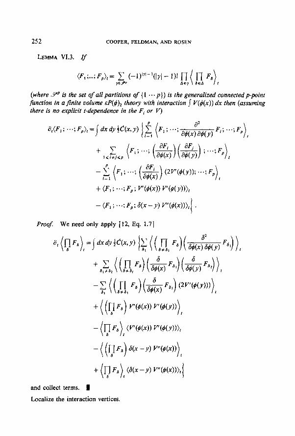
LEMMA VI.3. If
(F, ;...; F,), = y; P WY”-‘(lrl- I)! n ( Is 6) AMY SEA I
(where .Yp is the set of all partitions of { 1 .a. p)) is the generalized connected p-point function in a finite volume &P(d)* theory with interaction I V@(x)) dx then (assuming there is no explicit t-dependence in the Fi or V)
- F 1,
* . . . . W’“($(Y)); -;Fp) t
+ (F,; *es; Fp; HO) ~My>))t
- (F, ; . . . . Fp ; 6(x -Y> J?#(x)>)t I
-
ProoJ We need only apply [ 12, Eq. 1.71
and collect terms. 1
Localize the interaction vertices.

LEGENDRE TRANSFORMS 253
Let us stop to see where we stand. We have a sum of terms. If we consider any fixed set of localizations (they will be summed over later) we have a large finite number (depending only on n and m) of terms each of which is of the form (F, ; ...; F,), where F, contains the original J’s and L’s and F, . . . F, (p < m) arose from repeated application of Lemma VI.3. More precisely.
(a) F, contains all the J’s and L’s and all the interaction vertices produced by the contraction phase (Step 3). Every J and both arguments of every L is connected to such an interaction vertex without any intervening propagators. The total number of J’s and arguments of L’s connected to each such vertex must be at least one and at most the degree of the interaction. It is of course possible but not necessary for the two arguments of an L to be connected to different vertices. F, may also contain some interaction vertices produced by the a, phase (Step 4). Every such interaction vertex must be connected to some J or L by a string of (5 propagators as in, for example,
(b) Fi( 1 < i <p) contains only interaction vertices produced by the 8, phase (Step 4). All interaction vertices in each fixed Fi (1 < i <p) are connected to all other vertices in the same Fi by strings of C propagators.
We will need to exploit the connectedness properties of (F, ; --. ; F,), in the cluster expansion in order to get the decay factors which will enable us to sum over the localizations of the interaction vertices. To do so we use Ginibre’s duplicate field trick yet again. We take p copies of our current theory (with all its shades of colours r, y1 ,..., b,). We will label these copies by a “hue” index 1 < h <p. Then if w is a primitive pth root of unity
(See [ 15, Section IV.21.)
Step 5 (Cluster expansion estimate on one term). We will now use the cluster expansion to prove that each term produced in Steps 1-4 obeys the estimate
(6.2)
254 COOPER, FELDMAN, AND ROSEN
where ip is the set of indices of the L’s that had their arguments joined to distinct interaction vertices in Step 3 and E is a sum of products of decay factors with the number of terms in the sum depending only on n and m and with each product con- taining
(a) for every interaction vertex of F,,..., F,, produced in the 8, phase (Step 4) a factor e-““Ym’d’A9A’), where A is the localization of that interaction vertex and A’ is the localization of some f or L argument.
(b) for each J and L argument a factor e-rd(A,A’), where A is the localization of that argument and A’ is the localization of an argument of a different J or L.
The cluster expansion is by now standard so we will only outline this application. (We recommend that the cluster expansion novice first read [ 121.) The cluster expansion says (in the notation of [ 121)
(f-5.3)
where G is a polynomial in the fields
( >* X
9= I, =
s(T) =
W) ar=
( )~,owj
is our finite volume approximation to ( ),
is any finite union of closed lattice squares containing the support of G,
{all lattice bonds that do not intersect the support of G),
{Tc 9 1 r finite, TC Int X, every connected component of 4(9\r) intersects the support of G),
I I w), = i
if bET
I if bE.9?\r ’
is a vector having one component for each nonzero s(r)b,
Lr a/aa(r),y is the unnormalized expectation in volume X all of whose covariances (i.e. all hues of all shades of all colours) have the boundary conditions given by m9
z, = (1 X,O~l 3 Z ~p,ax = C1 %v,scr, *
Each term in the expansion is estimated in the usual way. The Kirkwood-Salsburg equation is used to bound Z,w,,JZ, by e”(L)‘x’. The 8 derivatives are evaluated using [ 12, Eq. (1.7)]. The Schwarz inequality (with respect to the Gaussian measure) is then used to separate the interaction from the polynomial in the fields downstairs. The former factor is bounded by e o(1)lxI The Gaussian integral containing the latter .

LEGENDRE TRANSFORMS 255
is evaluated as a sum of graphs which are estimated as follows. Each graph is of the form
where xi is the position of an interaction vertex produced in Step 3, di is its localization, I’ is the set of indices of the L,‘s that had their arguments joined to distinct interaction vertices in Step 3 and k is a product of propagators. The Schwarz inequality is used to separate k from the J’s and L’s. /I kll: is a graph of the form conventionally seen in cluster expansions and is estimated as such yielding e”“‘.” x e-“‘mO’ir’E’ where E’ is a product of decay factors. In particular, each propagator introduced in the 3, phase (Step 4) contributes a factor which decays exponentially with the distance between the supports of the propagator’s arguments. ~l17Jj17L,l~, is estimated by the following generalization of Holder’s inequality [ 12, Lemma 9.2 1:
LEMMA V1.4.
(6.4)
where K is a Jinite index set
K,,,cK,
xK* = Ixk I k E K,},
for each k and cm S.t. kEK, l/q, = l/q (< l/q iflu,, has mass 1).
Proof. This inequality is easily verified by induction on I K /, applying Holder’s inequality to each integration in turn. 1
We can certainly guarantee that, at any vertex, 2 q/i + C q; ’ < 4 by choosing qi = 20, q1 = 20 for all 1 E 9 and q1 = D for all I& I;0 since the number of L’s with 1 E I at that vertex plus twice the number of L’s with 16Z Y’ at that vertex can be at most D, the degree of the interaction. Altogether the cluster expansion gives
Now using 112. Prop. 5.11 which states that the number of terms in the above sum having a given value of 1x1 is at most eK21X’, [ 12, Eq. 5.11 which states 2 /r/ >
/Xl - a,,.,,, (where an.m is the size of the support of F, Fz ..- F,) and the fact that

256 COOPER, FELDMAN, AND ROSEN
K(Q) may be made arbitrarily large by increasing the bare mass m,, we get (for a new constant C)
Here (Xlmin is the area of the smallest (XI occurring in a nonzero term of (6.3). To complete the proof of (6.2) we must show
E’e- lxlmin & E.
Pick from (6.3) any nonzero term having /X/ = IXlmin. As explained at the beginning of this step we need in E decay (a) from the localization of each interaction vertex introduced in Step 4 to the localization of some J or L argument and (b) from the localization of each J or L argument to the localization of some argument of a different J or L. This decay arises from two sources. The first is exponential decay of the propagators that were also introduced in Step 4. The second is e-lX1min = e-lx’. If A and A’ are connected by X (meaning that they lie in the same connected component of X) then d(A, A’) < fi/Xl an we may extract the decay factor from e-‘X’min. d (Note that since any decay rate e(n, m) > 0 will do we may extract from e--/X’min or from any given propagator any finite number (depending only on n and m) of decay factors.) Hence if we wish to demonstrate decay between two localizations we must connect them by a string of propagators and/or components of X. This is exactly what we will do. Consider any localization A of interest (i.e., of a J or L argument or of an interaction vertex introduced in Step 4). Define its sphere of influence to be the union of all connected components of X containing another localization of interest which may be connected to A by a string of propagators and/or components of X. The proof of (6.2) is then completed by observing that
(a) The sphere of influence of any interaction vertex must include the localization of a J or L argument. This is trivial if the interaction vertex lies in F,. (See property (a) of Step 4.) On the other hand the sphere of influence X,, of Fi (i > 2) must intersect the support of F, since otherwise (nf= ,(ci= i O*Fi,h))~,~(r) factorizes with one factor being
( n (it* whFi4 L,,,,, leSc(Z,...,pl ( ) u =c &+ZkS h) rI FLhr 1 <h&J iss x0,0(r)
=+ :I ,<Z<, dZl~~~)+‘s’h (n F*,,,)’ = 0. fES x0.0(r)
The second last equality follows from the fact that by “hue invariance” x1 <,,, cp ~“‘~““+‘~“‘(rI~~s Ft,nil.io,~(r) is independent of h. (Just use the change of variables

LEGENDRE TRANSFORMS 257
hi + hi + h (modp).) The last equality follows from the fact that, since w is a primitive pth root of unity, xi=, o’~“’ = 0.
(b) Every sphere of influence X0 must contain the localizations of arguments from at least two J and/or L’s. Otherwise (nf= ,(Ci= 1 WhFi,h))i,o(r) = 0 thanks to the colour symmetries implemented in Step 2. To see this firstly observe that if X,, intersects the support of Fi for some i > 2 it must contain all of the support of Fi by (b) of Step 4. Hence the part of the integrand living in X, that comes from Fz ... F, is, for some subset S c (2 ,..., p),
and is invariant under permutations of colours and shades. Secondly, review Step 2 briefly and observe that the part of the integrand living in X0 that comes from F, has the same colour symmetry as [#I (if X0 contains the localization of a single J), as ]#‘I (if X0 contains the localizations of both arguments of a single L) or as one argument of [d’] (if X, contains the localization of one argument of a single L). Thirdly, observe that [$I = 4, - 4, is odd under r H y so that if 3- is any function of the fields (like the interaction) and propagators that is symmetric under permutation of colours ([$ ]X);, = 0. Similarly, Ml = 9~4 - ‘&+,A - +%BI, + 2#,#, with 04 - tiy& odd under r H y and 2$,$, - 2#,4, odd under r ++ b so that ([#]7);o = 0. F’ ma 11 y, suppose the expectation (.)1; factors into (.)f;,(.)f;, with the X0 factor containing one of the fields in a [#] and none of the other original fields. Then this expectation can be written as a sum of three terms,
each of which vanishes since ,% is symmetric under permutations of colours and. r, is symmetric under y c) b (the other [#4], s in Lc having been assigned a different shade of y and b).
Step 6 (Show (6.2) implies (6.1)). Firstly observe that we can use E to sum over the localizations of interaction vertices to give
layy:(nqk(t>-‘Jj)(n~qK(t)-‘L,C(t)-’$b~):),~
G I CE(Iajl, {all> I7 IIJj.ajII n IlL~,,,lL ni j 1 (6.5)
where
II4 = IIJll2D;*,
IlL II = l/Ll/*o;2 + IwdllD:2

258 COOPER, FELDMAN, AND ROSEN
and we have made explicit the formerly suppressed notation giving the localizations of J and L. Hence now
Jj,aj = JjXd, 3
L1.q = Xd,fXA,J *
The decay factor has become
E({aj}, {q}) = 1 n exp{-s(n, m) 44, aZ:j;$J, 0.7 I(i<n
IGk<2
where a,! = a: = ai for J localizations and c and r run over all maps
5: {(hk)J-t {L2},
u: {(i, k)} -+ { 1, 2 )...) n} o(i, k) z i.
This is just a fancy way of saying there must be decay from the localization of each J and L argument to the localization of a different J or L. We must bound the right hand side of (6.5) by C nj IlJjll n, llLlll f or some new constant C. Since E contains a finite number (depending only on n) of terms we need only consider one of them (i.e., one fixed but arbitrary o and r). Our estimate is simply an application of (U,A,A, a** A,,u,) < IIulII IIA,il ..a llA,,ll llv211 where u,, u2 E G and the Ats are operators between 12(Z2k)‘s for various values of k. (We identify 12(Z2”) and C.) The hardest part of the application is to organize
C n exp{ -s(n, m) d(a:, 431 n IIJj,,II n IIL,,a,ll ai i,k i I
properly. To do so we think of this expression as a graph which we construct as follows.
(1) Each IIJj,a,ll (llLl.,ll) is represented as a box with one (two) dot(s) on its boundary. Each dot represents one component of a.
(2) These boxes are arranged in a line. (3) Each factor e-~(~~~)~(~b$j~;(:) is represented as an edge joining the dots
associated with 4 and a;$;$. A typical such graph is
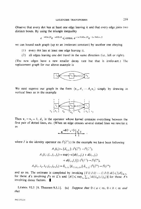
LEGENDRETRANSFORMS 259
Observe that every dot has at least one edge leaving it and that every edge joins two distinct boxes. By using the triangle inequality
e -d(a.4)e-cd(4,Y) < const* e -(f/2)d(n.0’e-.“,‘2’d’“,“’
we can bound each graph (up to an irrelevant constant) by another one obeying
(1) every dot has at least one edge leaving it.
(2) all edges leaving one dot travel in the same direction (i.e., left or right).
(The new edges have a new smaller decay rate but that is irrelevant.) The replacement graph for our above example is
We next express our graph in the form (v,,A, .e. A,vz) simply by drawing in vertical lines as in the example
Then v, = v2 = 1, A, is the operator whose kernel contains everything between the first pair of dotted lines, etc. (When an edge crosses several dotted lines we rewrite it as
-d(* ,*>;I; I Le.
I 8
where Z is the identity operator on f*(H*).) In the example we have been following
A ,(i,) = 113,,,1 jl: 12(Zo) -+ I’(Z”),
AAil ;j,J,,j,) = ev--E[d(i,.j,) + dG, ,jJ
+ d(i,,j,)j}: /‘(Z2)-* /2(26),
and so on. The estimate is completed by invoking (/I@ Z @ , . . @ Z (3 A I( < J/A (/H,S. for those A’s involving J’s or L’s and IIAII < supi,,, xi, IA((i,}; (j,})l for those A’s involving decay factors. 1
LEMMA VI.5 19, Theorem 9.5.11. (a) Suppose that 0 < a < co, 0 < b < co and that
59s: 13112-4

260 COOPER, FELDMAN, AND ROSEN
I
I/O r - ess sup Ik(t, s)l” da(s) = M, < 03,
l/b (5 - ess sup (k(t, s)l” dr(t)
I = M, < co.
(6.6)
(6.7)
Then k is the kernel of a continuous linear map from Lp(S, a) into Lq(T, r) whenever
and then 11 k/J < II~:-“‘~M~‘~,
(b) Suppose that 1 < b < a and that (6.7) holds. Then k is the kernel of a continuous linear map from L’(S, u) to Lb(T, 5) with (1 kJ[ <IV,.
(a’) Suppose that a(S) and t(T) are finite and that (6.6) and (6.7) hold with 0 < a < 00, 0 < b < 00. Then k is the kernel of a continuous linear map from Lp(S, a) to Lq(T, r) whenever there exists q, > q satisfying
(b’) Suppose that o(S) and t(T) are finite and that (6.7) holds with 1 ,< b < 03. Then k is the kernel of a continuous linear map from L ‘(S, u) into Lq(T, z) whenever 0 < q < b and then /I k, /I < M2r(T)“q-“b.
REFERENCES
1. M. BIRMAN AND M. SOLOMJAK, Vestnik LSU Math. 2 (1975). 9. F. HOLLAND, J. London Math. Sot. 10 (1975), 295.
2. A. COOPER, J. FELDMAN, AND L. ROSEN, Legendre transforms and r-particle irreducibility in quantum field theory: The formalism for r = 1,2, Ann. Phys. (N.Y.) 137 (1981), 146-209.
3. A. COOPER, J. FELDMAN, AND L. ROSEN, Higher Legendre transforms and their relationship to Bethe-Salpeter kernels and r-field projectors, J. Muth. Phys., in press.
4. A. COOPER, J. FELDMAN, AND L. ROSEN, Cluster irreducibility of the third and fourth Legendre transforms in quantum field theory, preprint.
5. A. COOPER, J. FELDMAN, AND L. ROSEN, Legendre transforms and r-particle irreducibility for the Yukawo model, in preparation.
6. A. COOPER, J. FELDMAN, AND L. ROSEN, The Second Legendre Transform for the Weakly Coupled P(#)2 Model, in preparation.
7. C. DE DOMINICIS AND P. MARTIN, J. Math. Phys. 5 (1964), 14-30; 31-59. 8. J. DIMOCK AND J. GLIMM, Aduan. in Math. 12 (1974), 58. 9. R. EDWARDS, “Functional Analysis,” Holt, Rinehart & Winston, New York, 1965.
IO. J. GLIMM AND A. JAFFE, Ann. Inst. H. Poincure Sect. A 21 (1974), 1. I I. J. GLIMM AND A. JAFFE, Commun. Math. Phys. 44 (1975), 293. 12. J. GLIMM, A. JAFFE, AND T. SPENCER, in “Constructive Quantum Field Theory” (G. Velo and A.
Wightman. Eds.), Lecture Notes in Physics No. 25, pp. 199-242, Springer, Berlin, 1973.

LEGENDRE TRANSFORMS 261
3. B. SIMON. “Trace Ideals and Their Applications.” Cambridge Univ. Press, London. 1979 4. T. SPENCER. C~mmun. Math. Phys. 44 (197S), 143. 5. G. SYLVESTER, “Continuous Spin Ising Ferromagnets,” M.I.T. Thesis, 1976. h. A. VASIL’EV AND A. KAZANSKII. Theor. Math. Phys. 12 (1972). 875.
Yu. M. PIS’MAK. Theor. Math. Phys. 18 (1974). 211. A. V,~SII.‘EV. A. KAZANSKII, AND Yu. M. PIS’MAK. Theor. Math. Phys. 20 (1974). 181.