Chapter 6

Color

Tuesday, Sept. 10, 2013 MIT EECS course 6.869, Bill Freeman and Antonio Torralba

Figure 6.1: Mixing of the colors of cleaning fluids: The blue-green of Windex and the yellow of Joymake green.

My first experience with color science happened when I was a child. I placed my yellow ski gogglesover a light blue bedspread and saw a color different than either of those two– green! It was magical.(The scene is re-enacted in Fig. 6.1 using cleaning fluids. Aswe’ll see from our analysis shortly, thelight blue bedspread would probably better be called “cyan”). Color theory is a wonderful mixture of

1

mathematics and aesthetics.Why do we need color vision? People with color deficits can be unaware of their deficiencies relative

to other peoples’ visual systems and can function just fine inthe world. Yet color makes vision mucheasier: it lets us isolate objects in front of backgrounds, infer physical properties of foods and surfaces(check whether fruit is ripe), and tell whether our childrenare sick by looking at the color of their skin.

We’ll first describe the physics of color, then discuss our perception of it–the physiology and psychophysics–, and finally address how we make inferences about the world from color measurements.

6.1 Color physics

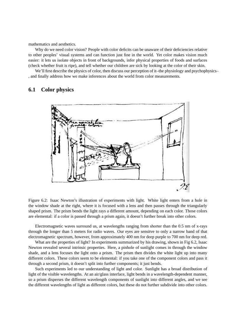
Figure 6.2: Isaac Newton’s illustration of experiments with light. White light enters from a hole inthe window shade at the right, where it is focused with a lens and then passes through the triangularlyshaped prism. The prism bends the light rays a different amount, depending on each color. Those colorsare elemental: if a color is passed through a prism again, it doesn’t further break into other colors.

Electromagnetic waves surround us, at wavelengths rangingfrom shorter than the 0.5 nm of x-raysthrough the longer than 5 meters for radio waves. Our eyes aresensitve to only a narrow band of thatelectromagnetic spectrum, however, from approximately 400 nm for deep purple to 700 nm for deep red.

What are the properties of light? In experiments summarizedby his drawing, shown in Fig 6.2, IsaacNewton revealed several intrinsic properties. Here, a pinhole of sunlight comes in through the windowshade, and a lens focuses the light onto a prism. The prism then divides the white light up into manydifferent colors. These colors seem to be elemental: if you take one of the component colors and pass itthrough a second prism, it doesn’t split into further components; it just bends.

Such experiments led to our understanding of light and color. Sunlight has a broad distribution oflight of the visible wavelengths. At an air/glass interface, light bends in a wavelength-dependent manner,so a prism disperses the different wavelength components ofsunlight into different angles, and we seethe different wavelengths of light as different colors, butthese do not further subdivide into other colors.

(a)

(b)

Figure 6.3: (a) A spectrograph constructed using a compact disk (CD). Light enters through a slit at theright, diffracting from the narrowly spaced lines of the CD.(b) Photograph of diffraction pattern fromsunlight, seen thorugh hole at bottom left.

Another simple experimental set-up to reveal the spectrum of light, using very accessible parts, isthe CD spectrometer depicted in Fig. 6.3 (a). Light passes through the slit at the right, and strikes a CD(with a track pitch of about 1600 nm). Constructive interference from the light waves striking the CDtracks occurs at a different angle for each wavelength of thelight, yielding a separation of wavelengthsby diffracting angle. The diffracted light can be viewed or photographed through the hole at the bottomleft. (For construction details and more examples, see thisvery nice web page:

http://www.cs.cmu.edu/˜zhuxj/astro/html/spectromete r.html

6.1.1 Radiometry and simplified reflection model

We can characterize the light by its power at each of the visible wavelengths, Fig. 6.4 shows a number ofdifferent light sources, and the spectra of the light they emit.

Light interacting with matter

We see through the interaction of light with matter. When light strikes a surface, it re-radiates with a dis-tribution of directions and intensities at each wavelengththat depends on the properties of the reflectingsurface. The distribution of the outgoing light also depends on properties of the incoming light, one ofthe many reasons why vision is difficult.

We can summarize the changes to the light upon surface reflection with a “bi-directional reflectancedistribution function”, or BRDF. The function is called “bi-directional” because it depends on both thedirection of the light incident on the surface and on the direction of the reflected light being characterized.The BRDF of a surface characterizes, for each wavelength, the fractional change in the spectral power oflight reflecting off the surface as a function of the angle of incidence of the light to the surface, and theviewing (reflection) angle. Shiney surfaces reflect most of the light into a single angle. Diffuse surfacesscatter the light broadly over a hemisphere of directions.

(a) (b)

(c)

(d)

Figure 6.4: (a) and (b): Plots of the power spectra of blue skyand a tungsten light bulb. Photographsshow (c) a flourescent light and (d) its spectrum as viewed with the spectrograph of Fig. (6.3) (a).

In this chapter, to simplify our study of surface appearance, we will ignore many of the rich de-tails of the BRDF. We will assume that the observed power spectrum of the reflected light does notdepend on either the angles of incidence or reflection from the surface. That is commonly the case fordiffuse reflections Under such conditions, the power spectrum of the reflected light,R(λ), is simply awavelength-by-wavelength product of the illumination power spectrum,I(λ) and the surface reflectancespectrum,S(λ):

R(λ) = I(λ)S(λ) (6.1)

Wavelength-by-wavelength multiplication is also a good model for spectral changes to light caused byviewing light through an attenuating filter. The incident power spectrum is multiplied at each wavelengthby the transmittance spectrum of the filter.

Even the simple model of Eq. (6.1) describes a rich visual world and allows us to make usefulinferences.

(a)(b)

(c)(d)

Figure 6.5: Some real-world objects and the reflected light spectra (photographed using Fig. (6.3) (a))from outdoor viewing. (a) Leaf and (b) its reflected spectrum. (c) A red door and (d) its reflectedspectrum.

(a)(b)

(c) (d)

Figure 6.6: More real-world objects and the reflected light spectra. (a) Blue-green chair and (b) itsreflected light. (c) Toby the dog and (d) his reflected spectrum.

Figure 6.7: Observed spectra of light reflecting off the surface. Source: Forsyth and Ponce, ComputerVision, Prentice Hall.

6.1.2 Color appearance of various spectra

Figure 6.4 (a) shows some example illumination spectra. Thespectrum of blue sky is on the left, andthe spectrum of a tungsten light bulb (which will look orangish) is on the right. Some reflectance spectraare in Figure 6.7. A white flower reflects spectral power almost equally over all visible wavelengths. Ayellow flower reflects in the green and red.

6.1.3 Cartoon Color Spectra

It’s helpful to develop the skill of being able to look at a light power spectrum and to know roughly whatcolor that spectrum would correspond to. Here is a rough description of what wavelengths correspondto what perceived colors, with a reference spectrum showingroughly what each individual wavelength,viewed by itself, looks like. (An engineer at the photographic company, Polaroid, showed this to me. Ithink of it as a cartoon color model, a hard-edged approximation to a much softer reality). The visiblespectrum lies roughly in the range between 400 and 700 nm. We can divide into three one-hundred nmbands, which, from short to long wavelengths, corresponds to blue, green, and red (again, speaking inbroad strokes). These are often called the additive primarycolors, which we’ll write more about.

White light is a mixture of all spectral colors. There are three other possible combinations of thethree one-hundred nm bands of wavelengths, and each can be associated with a color name: Cyan is amixture of blue and green, or roughly spectral power between400 and 600 nm. In printing applications,this is sometimes called “minus red”, since it is the full spectrum, with the red band subtracted. Blue andred, or light in the 400-500nm band, and in the 600-700nm band, is called magenta, or minus green. Redand green, with spectral power from 500-700 nm, make yellow,or minus blue.

Figure 6.8: Cartoon model for the reflectance spectra of observed colors

6.1.4 Why color is useful

Here is why color is useful: it tells us something about surfaces in the world. For example, assume wehave a white light source shining on a yellow egg. The light reflected from the egg, returning to the eye,will be yellow, letting us know, from a distance something about the properties of the egg’s surface (thatit’s yellow).

Let’s pose a problem that we’ll address later in the chapter:given that we only observe the product ofthe illumination and reflection spectra, how do we know whether we are observing a white egg, viewedunder yellow illumination, or a yellow egg, viewed under white illumination? See Fig. 6.23.

Before we address color appearance, we continue with two more issues with the physical propertiesof light spectra: color mixing, and low-dimensional models.

6.1.5 Color mixing

A light of one spectrum and color, shining on a surface of another color spectrum produces a third colorwhose spectrum is the wavelength-by-wavelength product ofthe two colors, as described by Eq. (6.1).This can be thoughtof as a form ofcolor mixing, where the illumination color and the surface reflectancecolor mix to form the color of the reflected light.

There are two different ways that spectra combine when we mixcolors together. While the preciseway two spectra combine may depend on the details of the corresponding physical process, these twomethods are a good model for many physical processes.

The first way is called additive color mixing. This is the way spectra combine when you project twolights simultaneously, so they are summed in our eye. CRT color televisions, DLP projectors, and colorsviewed very closely in space or time all exhibit additive color mixing. The spectrum of the mixed coloris a weighted sum of the spectra of the individual components. In the additive color mixing model, inour cartoon color model, red and green combine to give yellow.

The second way colors combine is called subtractive color mixing, but might make more sense to becalled multipliciative color mixing. This is the mixing of light reflecting off a surface. Under this mixingmodel, the spectrum of the combined color is proportional tothe product of the mixed components. Thiscolor mixing occurs when light reflects off a surface, or passes through a sequence of attenuating spectralfilters, such as with photographic film, paint, optical filters, and crayons. An example of color mixingunder the subtractive model, cyan and yellow combine to givegreen, since the cyan filter attenuates thered components of white light, and yellow filter would removethe remaining blue components, leavingonly the green spectral region of the original white light.

Figure 6.9 shows the cartoon spectra of these color mixing examples.

(a)(b)

Figure 6.9: Examples of color mixing, in the world of cartooncolor spectra. (a) In additive mixing, redand green combine to give yellow. (b) Under subtractive mixing, cyan and yellow mix to give green.

6.1.6 Low-dimensional models for spectra

Before we turn to color perception, let’s introduce a mathematical model for light spectra that makesthem much easier to work with. In general, when modeling the world, we want to keep everything assimple as possible, and that usually means working with as few degrees of freedom as possible. Colorspectra seem like relatively high-dimensional objects, since we can pick any combination of numbers,from 400 to 700 nm, as we’d like. Even sampling only every 10 nmof wavelength, that gives us 31numbers for each spectrum.

It turns out that for many real-world spectra, those 31 numbers are not independent and in practisespectra have far fewer degrees of freedom. It is common to uselow-dimensional linear models to approx-imate real-world reflectance and illumination spectra. Anygiven spectrum, sayS(λ), is approximatedas some linear combination of “basis spectra”,u(λ). For example, a 3-dimensional linear model ofS(λ)would be

...S(λ)

...

≈

......

...u1(λ) u2(λ) u3(λ)

......

...

ω1

ω2

ω3

(6.2)

The basis spectra can be found from a collection of training spectra. If we write the training spectraas columns of a matrix,D, then performing a singular value decomposition onD yields

D = U ∗ Λ ∗ V ′ (6.3)

whereU is a set of orthonormal spectral basis vectors,Λ is a diagonal matrix of singular values, andV ′

is a set of coefficients. The firstn columns ofU are then basis spectra that can best approximate thespectra in the training set, in a least squares sense.

Figure 6.10 shows a demonstration, with a particular collection of surface reflectance spectra,ui(λ)that this works quite well. The “Macbeth Color Checker”, a tool of color scientists and engineers, is astandard set of 24 color tiles, always made the same way Figure 6.10 (a). (So iconic that this woman,Figure 6.10 (b), a dedicated color scientist, I presume, hastatooed a Macbeth color checker on her arm!Alas, I’m sure the tatoo colors can only be an approximation to the real Macbeth colors).

The reflectance spectra of each Macbeth color chip has been measured. The first four basis spectra,calculated using the measured reflectance spectra and Eq. (6.3), are shown in Figure 6.10 (c). The rowsof Figure 6.10 (d) show the Macbeth color checker spectra, asoptimally approximated by 1, 2, and 3basis functions, respectively. The spectra are pretty wellapproximated by a 3-dimensional linear model,as you can see from the plots.

(a)

(b)

(c) (d)

Figure 6.10: (a) The Macbeth color checker, of such iconic status that a woman (b) has tatooed it on herarm. The bottom two figures are from Foundations of Vision, byBrian Wandell, Sinauer Assoc., 1995(c) Basis functions from which the Macbeth color checker reflectance spectra can be approximated, in(d), using 1, 2, and 3 basis functions (each row of (d), bottomto top).

6.2 Color measurement: assigning categories and numbers tocolor spec-tra

Now, we turn to the measurement of color appearance. Do all people peceive colors in the same way? Notall human languages divide up the space of all colors in the same groupings, which, in principle, couldimply differences in perception among those different human groups. For example, some languages,which tend to be spoken by people at high northern latitudes,divide up the colors that English speakerscall “blue” into a finer set of categories,

http://www.nature.com/news/2007/070430/full/news070 430-2.html.

There may be cultural or physiological reasons why people living in such locations would form finercategories of particular color shades.

Figure 6.11: English speakers lump all these shades into “blue”, while Russian speakers put them intotwo different verbal categories.

Despite these differences across languages, it turns out that most humans match colors very consis-tently and one can reliably assign numbers that predict color matches.

If you can assign coordinates to a color percept, there are a wealth of applications. You can build amachine to display colors that match some desired output. You can ensure that the colors of manufactureditems are consistent. Companies can trademark colors, so weneed to be able to specify what is beingtrademarked. We have color standards for foods, for example. Figure 6.12 shows a chart showing frenchfry color standards, one among many standards for food colors.

To see how to quantify colors, we first need to understand the machinery of the eye.

Figure 6.12: French fries color standard

6.2.1 The machinery of the eye

Given that spectra are generally low-dimensional, an organism doesn’t need a large number of spectralmeasurements to measure natural spectra. For our color vision, our eyes have three different classesof photoreceptors, which determines the fact that there arethree primary colors, three color layers inphotographic film, three colors of dots on a display screen, and why two color coordinates are needed tospecify any color, independent of its overall intensity (three color dimensions, minus one for the overallcolor normalization).

What is the machinery of human vision? Here is a drawing of therod and cones of the eye, and someof the nerve cells connecting them. The tall ones are the rodsand the short ones are the cones, both at thetop layer. By the way, where does the light come in, in this drawing? Differently than how you or I mightdesign things, the light comes in at the bottom, passes through the nerve fibers and blood vessels, thenreaches the photosensitive detectors at the top of the image. Evolution may have determined that thereare benefits to having the photodetectors on the inside, where they can more easily receive nourishmentfrom blood vessels.

The retina consists of 3 classes of color receptors. Figure 6.13 (b) shows the variability of thenumbers and spatial layout of color receptors (the red, green, and blue of the figure is *much* moresaturated than the spectral sensitivities of the cone receptor classes are). The 3 cone classes are denotedL, M, and S, for whether they are sensitive to the long, middle, or short wavelengths of the visiblespectrum. The spectral sensitivity curves are shown in Fig.6.13 (c).

In some sense, Fig. 6.13 (c) tells the whole story of spectrum-based color perception. Three detectors,with the spectral sensitivitiesRi(λ) shown here, signal their response to an incoming light spectrum,I(λ). The response,γi of a cone of color classi is

γi =

∫

λ

Ri(λ)I(λ)dλ (6.4)

This can be thought of as projection of the incoming light spectrum onto the three basis vectorsRi(λ),projecting the high-dimensional input spectrum onto a 3-dimensional subspace.

The fact that there are three different detectors means thatwe’ll 3 numbers to describe a perceivedcolor in the world ( or 2 numbers, if we normalize for intensity). The shapes of those curves tell uswhich real-world spectra will look the same to us (because they’ll give the same trio of photoreceptorresponses) and thus will tell us how make one color look like another one.

To help understand how color is measured, and the experiments that taught us what we know aboutcolor vision, let’s examine the psychophysical experiments that were done to learn what we know aboutcolor perception.

6.2.2 Color matching

Color perception measurement is mostly about color matching. We try to match a color with an additivecombination of a set of reference colors, typically called primary colors. Through experimentation, it hasbeen found that we can match the appearance of any color through a linear combination of three primarycolors, stemming from the fact that we have three classes of photoreceptors in our eyes.

In this section, we’re assuming that the color appearance isentirely determined by the spectrum ofthe light arriving at the eye. To ensure that this is true in the experiments, care must be taken to view thecolor comparisons under repeatable, controlled surrounding colors, because such details can influencethe color percept. We shine a controllable combination of the primary lights on one half of a bipartitewhite screen, and the test light on the other half, see Fig. 6.14 (a). A grey surround field is placed around

(a) (b)

(c)

Figure 6.13: (a) Drawing of the eye’s photoreceptors by the Spanish physiologist, Ramon y Cajal. (b)View of 9 different human foveas, with the cone receptor types (L, M, or S) marked (in R, G, and B,respectively). [citation below] (c) Spectral sensitivities of the L, M, and S cones.

The Journal of Neuroscience, 19 October 2005, 25(42): 9669- 9679; doi:10.1523/JNEUROSCI.2414-05.2005, Organization of the Hum an Trichromatic Cone Mosaic,Heidi Hofer, Joseph Carroll, Jay Neitz, Maureen Neitz, and D avid R. Williams

the viewing aperture, giving a view to the subject that lookssomething like that of the right hand side ofFig. 6.14 (a).

Finally, we arrive at how we can assign a number to any color: Pick a set of 3 lights, called pri-maries, and see what combination of these primaries is required to match any given color. This gives a(reproducible) representation for the color at the left: ifyou take these amounts of each of the selectedprimaries, you’ll match the input color.

What if our three selected primiaries don’t let us reach the test color? Fig. 6.14 (b) shows an exampleof that. It turns out we can always match any input test color if we “add negative light”, which means toadd positive light to the other side of the test comparison.

Human color matching has elegant properties that help us describe colors using linear algebra. Mostevery desirable linear property is satisfied with such colormatching experiments. Here’s one of them:if color A1 matches colorB1, and colorA2 matches colorB2, then the sum of colorsA1 andA2 willmatch the sum of colorsB1 andB2.

That tells us that if we represent a color by the amount of the 3primaries needed to make a match,or any number proportional to that, then we’ll be able to use anice vector space representation for color,where the observed linear combination laws will be obeyed.

That’s the psychophysics. We also have in the back of our heads the mechanistic view for howcolors generate signals in our brain: the light power spectrum gets projected onto the 3 photoreceptorclasses spectral sensitivity curves, generating three numbers, the L, M, and S cone responses, which arethe signal for that color. If we can adjust the primary color amounts,a1, a2, anda3, so that their sumgenerates the same set of photoreceptor signals when projected onto the photoreceptor spectral responsecurves, we have matched the color.

6.2.3 Linear algebraic interpretation of color perception

The psychophysics result leads to a linear algebraic interpretation of color. Let the space of all possiblespectral signals be N-dimensional. In this figure, we depictthat as a 3-dimensional space. The generationof cone response for a given spectral sensitivity curve can be thought of as projecting a N-dimensionalsignal onto a basis function and recording the resulting projection length. If we record the response of thethree different spectral sensitivity curves, we are measuring the projection of our N-d vector onto eachof three linearly independent basis vectors. Thus, a triplet of cone responses maps onto some coordinatein a 3-dimensional subspace (depicted as a 2-d plane here) ofthe original N-dimensional space.

Viewed that way, then the task of color measurement is simplythe task of finding the projection ofany of the possible N-d spectra into the special 3-d subspacedefined by the cone spectral response curves.Any basis for that 3-d subspace will serve that task. Equivalently, we seek to predict the cone responsesto any spectral signal, and projection of the spectral signal onto any 3 independent linear combinationsof the cone response curves will let us do that.

So we can define a color system by simply specifying its 3-d subspace basis vectors. And we cantranslate between any two such color representations by simply applying a general 3x3 matrix transfor-mation to change basis vectors. Note, the basis vectors do not need to be orthogonal, and most colorsystem basis vectors are not.

Long before scientists had measured the L, M, and S spectral sensitivity curves of the human eye,others had measured equivalent bases through psychophysical experiments. It is interesting to observehow such curves could be measured psychophysically.

(a)

(b)

(b)

Figure 6.14: (a) Color matching experiment (From Brian Wandell, Foundations of Vision, Sinauer, 1995).(b) Vector model for color matching experiment. Primary lights can synthesize a cone of possible colors.If a desired color to match is outside that cone, we can add a primary color to the test light until it isinside the feasible cone. Adding a light to the test light side, (c), is the same as subtracting it from theprimaries, but doesn’t require negative light intensity.

Color matching functions

Here’s what we can do to find such basis vectors, called “colormatching functions”, for any given set ofprimary lights. We exploit the linearity of color matching and find the primary light values contributingto a color match, one wavelength at a time. So for every pure spectral color as a test light, we measurethe combination of these three primaries required to color match light of that wavelength. For somewavelengths and choices of primaries, the matching will involve negative light values, and rememberthat just means those primary lights must be added to the testlight to achieve a color match.

Figure 6.15: Psychophysically measured color matching functions.

Figure 6.15 is an example of such a measured color matching function, for a particular choice ofprimaries, monochromatic laser lights of wavelengths 645.2, 525.3, and 444.4 nm. We can see thesematches are behaving as we would expect: when the spectral test light wavelength reaches that of one ofthe primary lights, then the color matching function is 1 forthat primary light, and 0 for the two others.

Because of the linearity properties of color matching, it’seasy to derive how to control the primarylights in order to matchany input spectral distribution,t(λ). Let the three measured color matchingfunctions beci(λ), for i = 1, 2, 3. Let the matrixC be the color matching functions arranged in rows,

C =

c1(λ1) . . . c1(λN )c2(λ1) . . . c2(λN )c3(λ1) . . . c3(λN )

(6.5)

Then, by linearity, the primary controls to yield a color match for any input spectrum~t =

t(λ1)...

t(λN )

will be∑

j Cijtj = C~t.So there is an infinite space of color matching basis functions to pick, so it’s natural to ask whether

any one choice of bases is better than another. One natural choice might be the cone spectral responsesthemselves, but those were only measured relatively recently, and many other systems were tried, andstandardized on, earlier.

(a)(b)

Figure 6.16: (a) CIE color matching functions. (b) The spaceof all colors (intensity normalized), asdescribed in the CIE coordinate system.

6.2.4 CIE color space

One standard you should know about, because it’s so common, is the CIE XYZ color space. Again, acolor space is simply a table of 3 color matching functions, which must be a linear combination of allthe other color matching functions, because they all span the same 3-d subspace of all possible spectra.The CIE color matching functions were designed to be all-positive at every wavelength. They’re shownin Fig. 6.16 (a). What might be the benefit of having an all-positive set of color matching functions? Ibelieve they were selected so that it would be simple to builda machine that used color filters of thosespectral responses to directly measure the color coordinates of a signal.

A bug with the CIE color matching functions is that there is noall positive set of color primary lightsassociated with those color matching functions. But if the goal is to simply specify a color from an inputspectrum, then any basis can work, regardless of whether there is a physically realizable set of primariesassociated with the color matching functions.

To find the CIE color coordinates, one projects the input spectrum onto the 3 color matching func-tions, to find coordinates, called tristimulus values, labeled X, Y, and Z. Often, these values are nor-malized to remove overall intensity variations, and one then calculatesx = X

X+Y+Zandy = Y

X+Y+Z.

Fig. 6.16 (b) shows the visible colors (intensity normalized) plotted in the CIE coordinatesx andy.

6.2.5 Color metamerism

One final topic for the model where power spectral density determines color is metamerism, when twodifferent spectra necessarily look the same to our eye. There is a huge space of metamers: any two vectorsdescribing light power spectra which give the same projection onto a set of color matching functions willlook the same to our eyes.

There’s a sense that our eyes are missing much of the possiblevisual action. There’s a high-dimensional space of colors out there, and we’re only viewing projections onto a 3-d subspace of that.

But in practise, the projections we observe do a pretty good job of capturing much of the interest-ing action in images. Given how much information is not captured by our eyes, hyperspectral images(recorded at many different wavelengths of analysis) add some, but not a lot, to the pictures formed by

our eyes.Let us summarize our discussion of color so far. Under certain viewing conditions, the perceived

color depends just on the spectral composition of light arriving at the eye (we move to more generalviewing conditions next). Under such conditions, there is asimple way to describe the perceived color:project its power spectrum onto a set of 3 vectors called color matching functions. These projections arethe color coordinates. We standardize on particular sets ofcolor coordinates. One such set is the CIEXYZ system.

How do you translate from one set of color coordinates to another, say, from the color coordinatesin a unprimed system to those in a primed system? Place the spectra of a set of primary lights into thecolumns of a matrixP. If we take the color coordinates,~x, as a 3x1 column vector and multiply themby the matrixP, we get a spectrum which is metameric with the input spectrumwhose color coordinateswere~x. So to convert~x to its representation in a primed coordinate system, we justhave to multiply thisspectrum by the color matching functions for the primed color system:

~x′ = C′P~x (6.6)

The color translation matrixC′P is a 3x3 matrix.

(a)

(b)

Figure 6.17: (a) The cone spectral sensitivity curves can bethought of as three basis vectors onto whichthe observed light spectrum is projected. This takes the input spectrum from a high-dimensional space(depicted as 3-d here) into a three-dimensional subspace (depicted as a 2-d plane here). Any two spectrawith the same projection into the 3-d subspace (with the samecone responses) will look the same. (b)Two spectra with the same projection onto the cone response curves, and a depiction of the two spectraas distinct points in the high-dimensional space of all possible power spectra, projecting onto the samepoint in the subspace of possible cone responses.

6.3 Other color coordinate systems

To measure color, we just need to describe point locations within the subspace of human cone responses,but we are free to use different projection bases that span that same 3d subspace. Once we have made theprojection into one coordinate system spanning that 3-d subspace, we are free to apply a 3x3 coordinatetransformation matrix to employ a different coordinate system. There are many such coordinate systemsthat have been used to describe colors.

6.3.1 RGB

There are many different standards for color bases called RGB (sRGB, Adobe RGB, etc). Here are thetransformation matrices between the CIE coordinates X, Y, Zdescribed above and sRGB:

R

G

B

=

3.24 −1.54 −0.50−0.97 1.88 0.040.06 −0.20 1.06

X

Y

Z

(6.7)

The inverse coordinate transformation is:

X

Y

Z

=

0.41 0.36 0.180.21 0.72 0.070.02 0.12 0.95

R

G

B

(6.8)

6.3.2 YIQ

It is often useful to have one color component correspond to grayscale, or luminance, image variations.A color basis that does this is the YIQ system, used in the old NTSC television standard. Here, Y isa luminance component (not the CIE Y component), and I and Q represent chromatic variations. Thetranslation from an RGB system is given here:

Y

I

Q

=

0.299 0.587 0.1140.596 −0.274 −0.3220.211 −0.523 0.312

R

G

B

(6.9)

6.3.3 Uniform color spaces

All the color systems described have a common drawback: equal perceptual differences between colorsdo not correspond to equal numerical distances in the color representations. Nonlinear transformationsare required to achieve that, typically a cube root. See

http://en.wikipedia.org/wiki/Lab_color_space

for the formulas.

6.4 Spatial Resolution and Color

One reason to transform between color coordinate systems isbecause of the human visual response todifferent colors. Figure 6.18 shows the contrast sensitivity to sinusoids of different spatial frequenciesfor a luminance (Y) grating, and two different color components (labeled R/Y and B/Y in the plot).

We are much more sensitive to variations in luminance, and this property is often exploited in imagecompression, processing, and display algorithms. Figures6.19 through 6.22 show the effect on the fullcolor image of blurring different color channels, within different color representations. Blurred chromaticcomponents have very little effect on the full-color image,while a blurred luminance component is quitenoticable.

Figure 6.18: Human spatial frequency sensitivity in R, G, B and L, a, b color representations

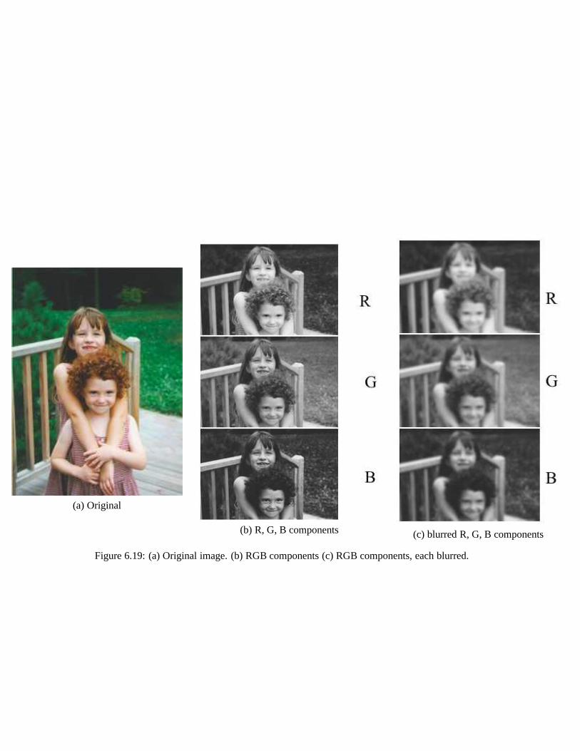
(a) Original

(b) R, G, B components (c) blurred R, G, B components

Figure 6.19: (a) Original image. (b) RGB components (c) RGB components, each blurred.

(a) R component blurred (b) G component blurred (c) B component blurred

Figure 6.20: (a) R component blurred, G and B components sharp. (b) G blurred, R and B sharp. Greenis the dominant component of the luminance signal, and blurring G has the most effect on the colorimage. (c) B blurred, R and G sharp.

(a) Original

(b) L, a, b components (c) blurred L, a, b components

Figure 6.21: (a) Original image. (b) Lab components (c) Lab components, each blurred.

(a) L component blurred (b) a component blurred (c) b component blurred

Figure 6.22: (a) L component blurred, a and b components sharp (big effect!). (b) a component blurred,L and b sharp. (c) b blurred, L and a sharp.

6.5 Color Constancy

Color perception depends strongly on the power spectrum of the light arriving at the eye, but it does notdepend only on that. Now we address the assumption that a given spectral power distribution alwaysleads to the same color percept.

In the demonstration of Fig. 6.24, identical spectral distributions arriving at your eye lead to differentcolor percepts. What’s going on? The eyes receive the product of the illumination and surface reflectancespectra, but the visual system may want to let us “see” the color of the surface color, independent ofthe spectrum of the illumination. So our visual system needsto “discount the illuminant” and presenta percept of the underlying colors of the surfaces being viewed, rather than simply summarizing theproduct spectrum arriving at the eye. The visual system usesthe context of the other colors is used toperform that calculation.

Figure 6.23: How do we distinguish an egg that is yellow because a yellow illuminant is falling on it,from a yellow egg?

The ability to perceive or estimate the surface colors of theobjects being viewed, and to not befooled by the illumination color, is called “color constancy”–you perceive a constant color, regardless ofthe illumination. People have some degree of color constancy, although not perfect color constancy.

For the case where there is just one illumination color in theimage, if we know either the illuminationspectrum or any of the surface color reflectance spectra, we can estimate the other from the data. So,from a computational point of view, you can also think of the color constancy task as that of estimatingthe illuminant spectrum from an image.

The rendering equation

Let’s examine the computation required to achieve color constancy. Here’s the rendering equation, show-ing, in our model, how the L, M, and S cone responses for thejth patch are generated:

Lj

Mj

Sj

= ET (A~xsj . ∗B~xi) (6.10)

In the above,Lj, Mj, andSj are the cone responses of thej patch of color. In this matrix equation, wedivide the visible spectrum intoN bins. The three rows of the Nx3 matrix,ET , are the spectral sensitivitycurves of the three cone classes. The columns of the matrixA are the surface reflectance spectra basisfunctions and~xsj contains the surface (s) reflectance basis function coefficients for thejth color patch.

(a) (b)

(c) (d) (e)

Figure 6.24: Color constancy demonstration (made by Prof. David Brainard, U. Penn) (a) a set of colors.(b) The “nothing up my sleeves” picture: the tiny blue squareat the left, and the large blue square at rightare made from the same filter material. If we cover some of the colors with the small blue square, thecolors change their appearance. (c) the white square (3rd row, 3rd column) goes to blue, and (d) orange(1st column, 5th row) goes to green-brown. (e) But if we coverall the colors with the large blue filter,the colors maintain their original appearance, for the mostpart. White stays white, orange stays orange.This is despite the fact that the same spectral signal is reaching your eye for those two patches as whenthe small blue squared covered each of them.

“.*” represents term-by-term multiplication. Similarly,The columns of the matrixB are the illuminationreflectance spectra basis functions and the vector~xij contains the illumination (i) spectral basis functioncoefficients.

Figure 6.25 shows a graphical diagram showing the vector andmatrix sizes in the above equation.We have some unknown illuminant, described by, say, a 3-dimensional vector of coefficients for theillumination spectrum basis functions. For thisjth color patch, we have a set of surface reflectancespectrum basis coefficients, let’s say also 3-dimensional.The term-by-term product of the resultingspectra (the quantity in parenthesis in the top equation) isour model of the spectrum of the light reachingour eye. That spectrum then gets projected onto spectral responsivity curves of each of the three coneclasses in the eye, resulting in the L, M, and S response for this jth color patch. (An equation for theRGB pixel color values would be the same, with just a different matrixE). If we makeN distinct colormeasurements of the image, then we’ll haveN different versions of this equation, with a different vector

~xsj and different observations

Lj

Mj

Sj

for each equation.

Figure 6.25: Graphical depiction of Eq. 6.10.

Like various other problems in vision, this is a bilinear problem. If we knew one of the two sets ofvariables, we could find the other trivially by solving a linear equation (using either a least squares or anexact solution). It’s a very natural generalization of the ab = 1 problem that Antonio talked about lastweek.

Let’s notice the degrees of freedom. We get 3 numbers for every new color patch we look at, but wealso add 3 unknowns we have to estimate (the spectrum coefficients~xsj), as well as the additional threeunknowns for the whole image, the illumination spectrum coefficients~xi. If only surface color spectrahad only two degrees of freedom, we’d catch up and potentially have an over-determined problem if wejust looked at enough colors in the scene. Unfortunately, 2-dimensional surface reflectance models justdon’t work well in practice, so that approach doesn’t work.

6.5.1 Some color constancy algorithms

So how will we solve this? Let’s look at two well-known simplealgorithms, and then we’ll look at aBayesian approach.

Bright equals white If we knew the true color of even a single color patch, we’d have the informationwe needed to estimate the 3-d illumination spectrum. One simple algorithm for estimating or balancingthe illuminant is to assume that the color of the brightest patch of an image is white. (If you’re workingwith a photograph, you’ll always have to worry about clippedintensity values, in addition to all the non-linearities of the camera’s processing chain). If that is thekth patch, and~xW are the known spectral basiscoefficients for white, then we have

~yk =

Lk

Mk

Sk

= ET (A~xW . ∗ B~xi) (6.11)

which gives a linear equation that we can solve for the unknown illuminant,~xi.How well does it work? It works sometimes, but not always. Thebright equals white algorithm

estimates the illuminant based on the color of a single patch, and we might expect to get a more robustilluminant estimate if we use many color patches in the estimate. A second heuristic that’s often used iscalled thegrey world assumption: the average value of every color in the image is assumed to begrey.

Figure 6.26: An image that violates the grey world assumption.

We take the sum over all samplesj on both sides of the rendering equation, Eq. (6.10). Letting~xG

be the spectral basis coefficients for grey, which we equate to the average of all the basis coefficients inthe image,1

M

∑

j ~xsj we have

1

M

∑

j

Lj

Mj

Sj

= ET (A

1

M

∑

j

~xsj . ∗ B~xi) (6.12)

= ET (A~xG . ∗ B~xi), (6.13)

where we have assumed there areM color patches in the image. Now, again, that leaves us with a linearequation to solve for~xi.

This assumption can work quite well, although, of course, wecan find images for which it wouldcompletely mess up, such as the forest scene of Fig. 6.26.

Using just part of the data (the brightest color, or even the average color) gives sub-optimal results.Why not use all the data, make a richer set of assumptions about the illuminants and surfaces in theworld, and treat this as aBayesian estimation problem? That’s what we’ll do now, and what you’llcontinue in your homework assignment.

To remind you, in a Bayesian approach, we seek to find the posterior probability of the state we wantto estimate, given the observations we see. We use Bayes ruleto write that probability as a (normalized)product of two terms we know how to deal with: the likelihood term and the prior term. Letting~x be thequantities to estimate, and~y be the observations, we have

P (~x|~y) = kP (~y|~x)P (~x) (6.14)

wherek is a normalization factor that forces that the integral ofP (~x|~y) over all~x is one.P (~x|~y) is theposterior probability–in this case, the probability of a vector~xi of illumination spectral basis coefficients,and of all the vectors~xsj of surface spectral basis coefficients, given the data,~y, of observationsLj, Mj,andSj from each color patchj. P (~y|~x) is called the likelihood term, andP (~x) is the prior probabilityof any given illuminant and set of surface reflectance basis spectra.

The likelihood term tells us, given the model, how probable the observations are. If we assume ad-ditive, mean zero Gaussian noise, the probability that thejth color observation differs from the renderedparameters follows a mean zero Gaussian distribution. Remembering that the observations~yj are the theL, M, and S cone responses,

~yj =

Lj

Mj

Sj

(6.15)

we have

P (~yj|~xi, ~xsj) =1√2πσ2

exp−|~yj − ~f(~xi, ~xsj)|2

2σ2, (6.16)

For an entire collection ofN surfaces, we have

P (~x|~y) = P (~xi)∏

j

P (~yj |~xi, ~xsj)P (~xsj) (6.17)

reminder: The rendering function,~f(~xi, ~xsj), comes from Eq. (6.10). We assume diffuse reflectionfrom each colored surface. Given basis function coefficients for the illuminant,~xi, and a matrixB withthe illumination basis functions as its columns, then the spectral illumination as a function of wavelengthis the column vectorB~xi. We also need to computejth surface’s diffuse reflectance spectral attenuationfunction, the product of its basis coefficients times the surface spectral basis functions:A~xsj In ourdiffuse rendering model, the reflected power is the term-by-term product (we borrow Matlab notation forthat, .*) of those two. The observation of thejth color is the projection of that spectral power onto theeye’s photoreceptor response curves. If those photoreceptor responses are in the columns of the matrix,E, then the forward model for the three photoreceptor responses at thejth color is:

~f(~xi, ~xsj) = ET (A~xsj . ∗ B~xi). (6.18)