Embed Size (px)
Citation preview
Clay Mathematics Proceedings
Volume 15, 2012
Lectures on Random Polymers
Francesco Caravenna, Frank den Hollander, and Nicolas Petrelis
Abstract. These lecture notes are a guided tour through the fascinatingworld of polymer chains interacting with themselves and/or with their envi-ronment. The focus is on the mathematical description of a number of physicaland chemical phenomena, with particular emphasis on phase transitions andspace-time scaling. The topics covered, though only a selection, are typicalfor the area. Sections 1–3 describe models of polymers without disorder, Sec-tions 4–6 models of polymers with disorder. Appendices A–E contain tutorialsin which a number of key techniques are explained in more detail.
Contents
Foreword 3191. Background, model setting, free energy, two basic models 3202. Polymer collapse 3283. A polymer near a homogeneous interface 3374. A polymer near a random interface 3455. A copolymer interacting with two immiscible fluids 3526. A polymer in a random potential 362Appendix A. Tutorial 1 369Appendix B. Tutorial 2 371Appendix C. Tutorial 3 375Appendix D. Tutorial 4 379Appendix E. Tutorial 5 385References 389
Foreword
These notes are based on six lectures by Frank den Hollander and five tutorialsby Francesco Caravenna and Nicolas Petrelis. The final manuscript was preparedjointly by the three authors. A large part of the material is drawn from the mono-graphs by Giambattista Giacomin [55] and Frank den Hollander [70]. Links are
2010 Mathematics Subject Classification. Primary: 60F10, 60K37, 82B26, 82D60; Secondary:60F67, 82B27, 82B44, 92D20.
c©2012 Francesco Caravenna, Frank den Hollander, Nicolas Petrelis
319
320 CARAVENNA, DEN HOLLANDER, AND PETRELIS
made to some of the lectures presented elsewhere in this volume. In particular,it is argued that in two dimensions the Schramm-Loewner Evolution (SLE) is anatural candidate for the scaling limit of several of the “exotic lattice path” modelsthat are used to describe self-interacting random polymers. Each lecture provides asnapshot of a particular class of models and ends with a formulation of some openproblems. The six lectures can be read independently.
Random polymers form an exciting, highly active and challenging field of re-search that lies at the crossroads between mathematics, physics, chemistry andbiology. DNA, arguably the most important polymer of all, is subject to severalof the phenomena that are described in these lectures: folding (= collapse), denat-uration (= depinning due to temperature), unzipping (= depinning due to force),adsorption (= localization on a substrate).
1. Background, model setting, free energy, two basic models
In this section we describe the physical and chemical background of randompolymers (Sections 1.1–1.4), formulate the model setting in which we will be working(Section 1.5), discuss the central role of free energy (Section 1.6), describe two basicmodels of random polymer chains: the simple random walk and the self-avoidingwalk (Section 1.7), and formulate a key open problem for the latter (Section 1.8).
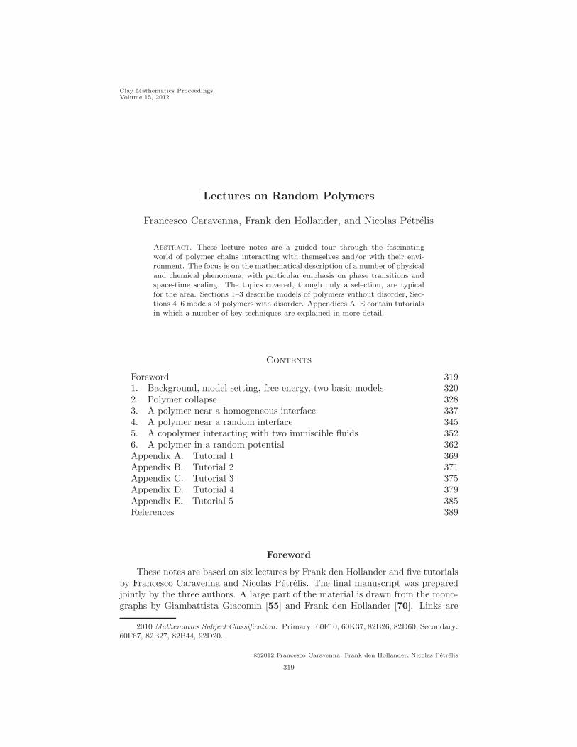
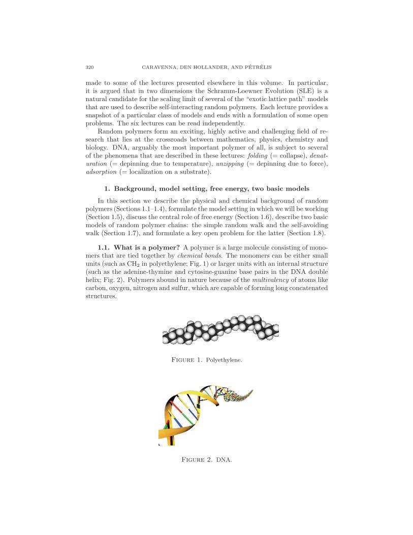
1.1. What is a polymer? A polymer is a large molecule consisting of mono-mers that are tied together by chemical bonds. The monomers can be either smallunits (such as CH2 in polyethylene; Fig. 1) or larger units with an internal structure(such as the adenine-thymine and cytosine-guanine base pairs in the DNA doublehelix; Fig. 2). Polymers abound in nature because of the multivalency of atoms likecarbon, oxygen, nitrogen and sulfur, which are capable of forming long concatenatedstructures.
Figure 1. Polyethylene.
Figure 2. DNA.
LECTURES ON RANDOM POLYMERS 321
1.2. What types of polymers occur in nature? Polymers come in twovarieties: homopolymers, with all their monomers identical (such as polyethylene),and copolymers, with two or more different types of monomers (such as DNA). Theorder of the monomer types in copolymers can be either periodic (e.g. in agar) orrandom (e.g. in carrageenan).
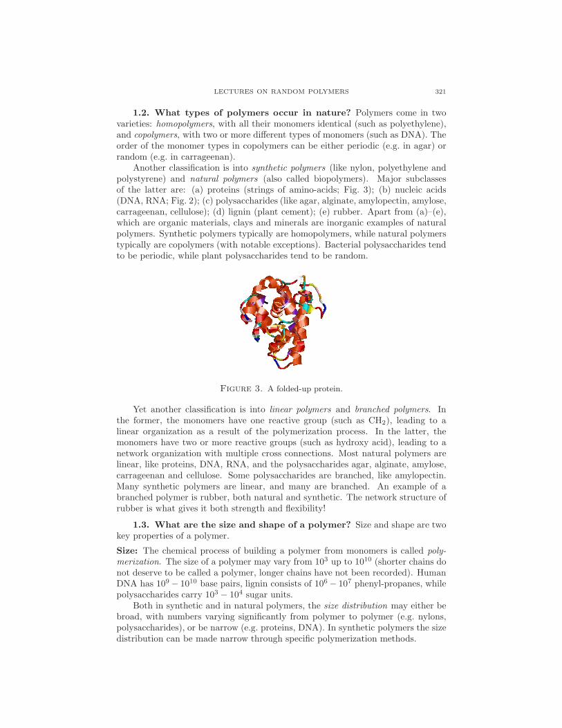
Another classification is into synthetic polymers (like nylon, polyethylene andpolystyrene) and natural polymers (also called biopolymers). Major subclassesof the latter are: (a) proteins (strings of amino-acids; Fig. 3); (b) nucleic acids(DNA, RNA; Fig. 2); (c) polysaccharides (like agar, alginate, amylopectin, amylose,carrageenan, cellulose); (d) lignin (plant cement); (e) rubber. Apart from (a)–(e),which are organic materials, clays and minerals are inorganic examples of naturalpolymers. Synthetic polymers typically are homopolymers, while natural polymerstypically are copolymers (with notable exceptions). Bacterial polysaccharides tendto be periodic, while plant polysaccharides tend to be random.
Figure 3. A folded-up protein.
Yet another classification is into linear polymers and branched polymers. Inthe former, the monomers have one reactive group (such as CH2), leading to alinear organization as a result of the polymerization process. In the latter, themonomers have two or more reactive groups (such as hydroxy acid), leading to anetwork organization with multiple cross connections. Most natural polymers arelinear, like proteins, DNA, RNA, and the polysaccharides agar, alginate, amylose,carrageenan and cellulose. Some polysaccharides are branched, like amylopectin.Many synthetic polymers are linear, and many are branched. An example of abranched polymer is rubber, both natural and synthetic. The network structure ofrubber is what gives it both strength and flexibility!
1.3. What are the size and shape of a polymer? Size and shape are twokey properties of a polymer.
Size: The chemical process of building a polymer from monomers is called poly-merization. The size of a polymer may vary from 103 up to 1010 (shorter chains donot deserve to be called a polymer, longer chains have not been recorded). HumanDNA has 109 − 1010 base pairs, lignin consists of 106 − 107 phenyl-propanes, whilepolysaccharides carry 103 − 104 sugar units.
Both in synthetic and in natural polymers, the size distribution may either bebroad, with numbers varying significantly from polymer to polymer (e.g. nylons,polysaccharides), or be narrow (e.g. proteins, DNA). In synthetic polymers the sizedistribution can be made narrow through specific polymerization methods.
322 CARAVENNA, DEN HOLLANDER, AND PETRELIS
The length of the monomer units varies from 1.5 A (for CH2 in polyethylene)to 20 A (for the base pairs in DNA), with 1 A = 10−10m.
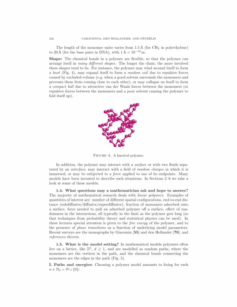
Shape: The chemical bonds in a polymer are flexible, so that the polymer canarrange itself in many different shapes. The longer the chain, the more involvedthese shapes tend to be. For instance, the polymer may wind around itself to forma knot (Fig. 4), may expand itself to form a random coil due to repulsive forcescaused by excluded-volume (e.g. when a good solvent surrounds the monomers andprevents them from coming close to each other), or may collapse on itself to forma compact ball due to attractive van der Waals forces between the monomers (orrepulsive forces between the monomers and a poor solvent causing the polymer tofold itself up).
Figure 4. A knotted polymer.
In addition, the polymer may interact with a surface or with two fluids sepa-rated by an interface, may interact with a field of random charges in which it isimmersed, or may be subjected to a force applied to one of its endpoints. Manymodels have been invented to describe such situations. In Sections 2–6 we take alook at some of these models.
1.4. What questions may a mathematician ask and hope to answer?The majority of mathematical research deals with linear polymers. Examples ofquantities of interest are: number of different spatial configurations, end-to-end dis-tance (subdiffusive/diffusive/superdiffusive), fraction of monomers adsorbed ontoa surface, force needed to pull an adsorbed polymer off a surface, effect of ran-domness in the interactions, all typically in the limit as the polymer gets long (sothat techniques from probability theory and statistical physics can be used). Inthese lectures special attention is given to the free energy of the polymer, and tothe presence of phase transitions as a function of underlying model parameters.Recent surveys are the monographs by Giacomin [55] and den Hollander [70], andreferences therein.
1.5. What is the model setting? In mathematical models polymers oftenlive on a lattice, like Z
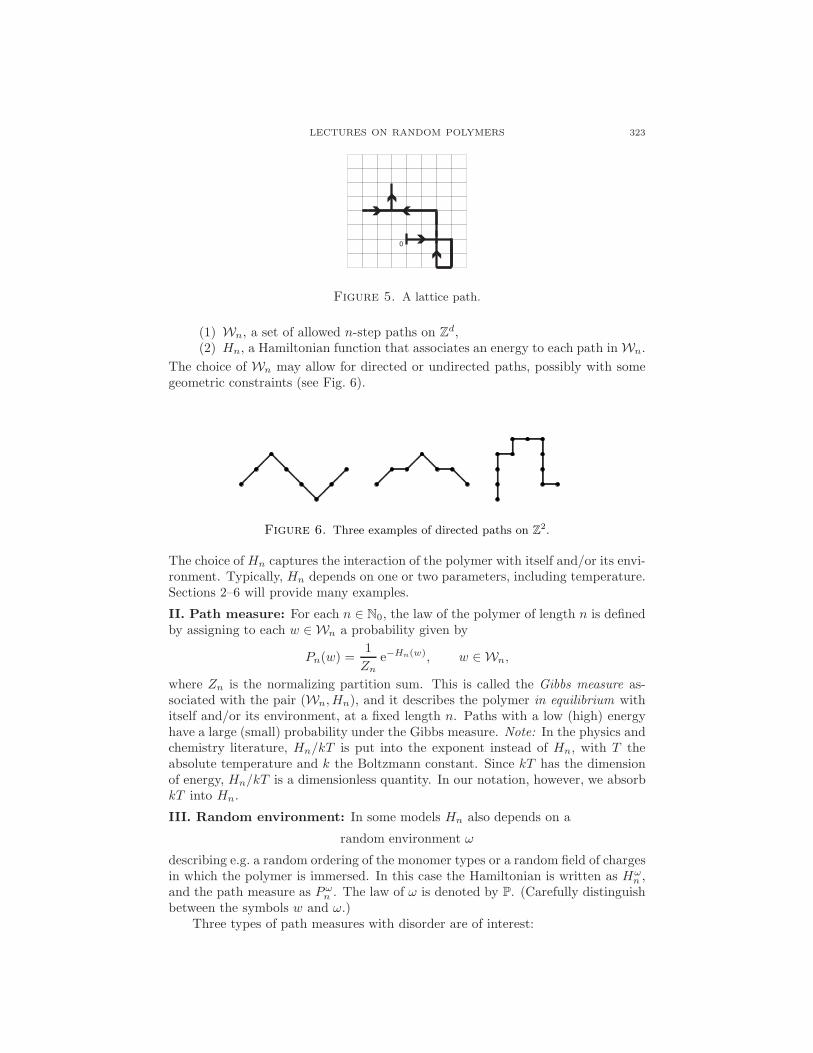
d, d ≥ 1, and are modelled as random paths, where themonomers are the vertices in the path, and the chemical bonds connecting themonomers are the edges in the path (Fig. 5).
I. Paths and energies: Choosing a polymer model amounts to fixing for eachn ∈ N0 = N ∪ 0:
LECTURES ON RANDOM POLYMERS 323
0
Figure 5. A lattice path.
(1) Wn, a set of allowed n-step paths on Zd,
(2) Hn, a Hamiltonian function that associates an energy to each path in Wn.
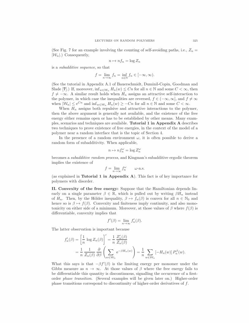
The choice of Wn may allow for directed or undirected paths, possibly with somegeometric constraints (see Fig. 6).
Figure 6. Three examples of directed paths on Z2.
The choice of Hn captures the interaction of the polymer with itself and/or its envi-ronment. Typically, Hn depends on one or two parameters, including temperature.Sections 2–6 will provide many examples.
II. Path measure: For each n ∈ N0, the law of the polymer of length n is definedby assigning to each w ∈ Wn a probability given by
Pn(w) =1
Zne−Hn(w), w ∈ Wn,
where Zn is the normalizing partition sum. This is called the Gibbs measure as-sociated with the pair (Wn, Hn), and it describes the polymer in equilibrium withitself and/or its environment, at a fixed length n. Paths with a low (high) energyhave a large (small) probability under the Gibbs measure. Note: In the physics andchemistry literature, Hn/kT is put into the exponent instead of Hn, with T theabsolute temperature and k the Boltzmann constant. Since kT has the dimensionof energy, Hn/kT is a dimensionless quantity. In our notation, however, we absorbkT into Hn.
III. Random environment: In some models Hn also depends on a
random environment ω
describing e.g. a random ordering of the monomer types or a random field of chargesin which the polymer is immersed. In this case the Hamiltonian is written as Hω
n ,and the path measure as Pωn . The law of ω is denoted by P. (Carefully distinguishbetween the symbols w and ω.)
Three types of path measures with disorder are of interest:

324 CARAVENNA, DEN HOLLANDER, AND PETRELIS
(1) The quenched Gibbs measure
Pωn (w) =1
Zωne−H
ωn (w), w ∈ Wn.
(2) The average quenched Gibbs measure
E(Pωn (w)) =
∫Pωn (w)P(dω), w ∈ Wn.
(3) The annealed Gibbs measure
Pn(w) =1
Zn
∫e−H
ωn (w)
P(dω), w ∈ Wn.
These are used to describe a polymer whose random environment is frozen [(1)+(2)],respectively, takes part in the equilibration [(3)]. Note that in (3), unlike in (2),the normalizing partition sum does not (!) appear under the integral.
It is also possible to consider models where the length or the configuration ofthe polymer changes with time (e.g. due to growing or shrinking), or to considera Metropolis dynamics associated with the Hamiltonian for an appropriate choiceof allowed transitions. These non-equilibrium situations are very interesting andchallenging, but so far the available mathematics is rather limited. Two recentreferences are Caputo, Martinelli and Toninelli [25], Caputo, Lacoin, Martinelli,Simenhaus and Toninelli [26].
1.6. The central role of free energy. The free energy of the polymer isdefined as
f = limn→∞
1
nlogZn
or, in the presence of a random environment, as
f = limn→∞
1
nlogZωn ω-a.s.
If the limit exists, then it typically is constant ω-a.s., a property referred to asself-averaging. We next discuss existence of f and some of its properties.
(a)
(b)
Figure 7. Concatenation of two self-avoiding paths: (a) the concate-nation is self-avoiding; (b) the concatenation is not self-avoiding.
I. Existence of the free energy: When Hn assigns a repulsive self-interactionto the polymer, the partition sum Zn satisfies the inequality
Zn ≤ Zm Zn−m ∀ 0 ≤ m ≤ n.
LECTURES ON RANDOM POLYMERS 325
(See Fig. 7 for an example involving the counting of self-avoiding paths, i.e., Zn =|Wn|.) Consequently,
n 7→ nfn = logZn
is a subadditive sequence, so that
f = limn→∞
fn = infn∈N
fn ∈ [−∞,∞).
(See the tutorial in Appendix A.1 of Bauerschmidt, Duminil-Copin, Goodman andSlade [7].) If, moreover, infw∈Wn
Hn(w) ≤ Cn for all n ∈ N and some C <∞, thenf 6= −∞. A similar result holds when Hn assigns an attractive self-interaction tothe polymer, in which case the inequalities are reversed, f ∈ (−∞,∞], and f 6= ∞when |Wn| ≤ eCn and infw∈Wn
Hn(w) ≥ −Cn for all n ∈ N and some C <∞.When Hn assigns both repulsive and attractive interactions to the polymer,
then the above argument is generally not available, and the existence of the freeenergy either remains open or has to be established by other means. Many exam-ples, scenarios and techniques are available. Tutorial 1 in Appendix A describestwo techniques to prove existence of free energies, in the context of the model of apolymer near a random interface that is the topic of Section 4.
In the presence of a random environment ω, it is often possible to derive arandom form of subadditivity. When applicable,
n 7→ nfωn = logZωn
becomes a subadditive random process, and Kingman’s subadditive ergodic theoremimplies the existence of
f = limn→∞
fωn ω-a.s.
(as explained in Tutorial 1 in Appendix A). This fact is of key importance forpolymers with disorder.
II. Convexity of the free energy: Suppose that the Hamiltonian depends lin-early on a single parameter β ∈ R, which is pulled out by writing βHn insteadof Hn. Then, by the Holder inequality, β 7→ fn(β) is convex for all n ∈ N0 andhence so is β 7→ f(β). Convexity and finiteness imply continuity, and also mono-tonicity on either side of a minimum. Moreover, at those values of β where f(β) isdifferentiable, convexity implies that
f ′(β) = limn→∞
f ′n(β).
The latter observation is important because
f ′n(β) =
[1
nlogZn(β)
]′=
1
n
Z ′n(β)
Zn(β)
=1
n
1
Zn(β)
∂
∂β
(∑
w∈Wn
e−βHn(w)
)=
1
n
∑
w∈Wn
[−Hn(w)]Pβn (w).
What this says is that −βf ′(β) is the limiting energy per monomer under theGibbs measure as n → ∞. At those values of β where the free energy fails tobe differentiable this quantity is discontinuous, signalling the occurrence of a first-order phase transition. (Several examples will be given later on.) Higher-orderphase transitions correspond to discontinuity of higher-order derivatives of f .
326 CARAVENNA, DEN HOLLANDER, AND PETRELIS
1.7. Two basic models. The remainder of this section takes a brief lookat two basic models for a polymer chain: (1) the simple random walk, a polymerwithout self-interaction; (2) the self-avoiding walk, a polymer with excluded-volumeself-interaction. In some sense these are the “plain vanilla” and “plain chocolate”versions of a polymer chain. The self-avoiding walk is the topic of the lectures byBauerschmidt, Duminil-Copin, Goodman and Slade [7].
(1) Simple random walk: SRW on Zd is the random process (Sn)n∈N0
definedby
S0 = 0, Sn =
n∑
i=1
Xi, n ∈ N,
where X = (Xi)i∈N is an i.i.d. sequence of random variables taking values in Zd
with marginal law (‖ · ‖ is the Euclidean norm)
P (X1 = x) =
12d , x ∈ Z
d with ‖x‖ = 1,
0, otherwise.
Think of Xi as the orientation of the chemical bond between the (i− 1)-th and i-thmonomer, and of Sn as the location of the end-point of the polymer of length n.SRW corresponds to choosing
Wn =w = (wi)
ni=0 ∈ (Zd)n+1 :
w0 = 0, ‖wi+1 − wi‖ = 1 ∀ 0 ≤ i < n,
Hn ≡ 0,
so that Pn is the uniform distribution on Wn. In this correspondence, think of(Si)
ni=0 as the realization of (wi)
ni=0 drawn according to Pn.
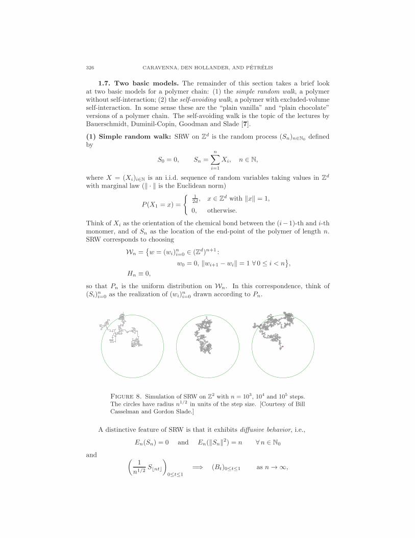
Figure 8. Simulation of SRW on Z2 with n = 103, 104 and 105 steps.
The circles have radius n1/2 in units of the step size. [Courtesy of BillCasselman and Gordon Slade.]
A distinctive feature of SRW is that it exhibits diffusive behavior, i.e.,
En(Sn) = 0 and En(‖Sn‖2) = n ∀n ∈ N0
and (1
n1/2S⌊nt⌋
)
0≤t≤1
=⇒ (Bt)0≤t≤1 as n→ ∞,

LECTURES ON RANDOM POLYMERS 327
where the right-hand side is Brownian motion on Rd, and =⇒ denotes convergence
in distribution on the space of cadlag paths endowed with the Skorohod topology(see Fig. 8).
(2) Self-avoiding walk: SAW corresponds to choosing
Wn =w = (wi)
ni=0 ∈ (Zd)n+1 :
w0 = 0, ‖wi+1 − wi‖ = 1 ∀ 0 ≤ i < n,
wi 6= wj ∀ 0 ≤ i < j ≤ n,
Hn ≡ 0,
so that Pn is the uniform distribution on Wn. Again, think of (Si)ni=0 as the
realization of (wi)ni=0 drawn according to Pn.
Figure 9. Simulation of SAW on Z2 with n = 102, 103 and 104 steps.
The circles have radius n3/4 in units of the step size. [Courtesy of BillCasselman and Gordon Slade.]
SAW in d = 1 is trivial. In d ≥ 2 no closed form expression is available forEn(‖Sn‖2), but for small and moderate n it can be computed via exact enumerationmethods. The current record is: n = 71 for d = 2 (Jensen [81]); n = 36 ford = 3 (Schram, Barkema and Bisseling [93]); n = 24 for d ≥ 4 (Clisby, Liang andSlade [36]). Larger n can be handled either via numerical simulation (presently upto n = 225 ≈ 3.3× 10⁷ in d = 3) or with the help of extrapolation techniques.
The mean-square displacement is predicted to scale like
En(‖Sn‖2) =Dn2ν [1 + o(1)], d 6= 4,
D n(logn)14 [1 + o(1)], d = 4,
as n→ ∞,
with D a non-universal diffusion constant and ν a universal critical exponent. Here,universal refers to the fact that ν is expected to depend only on d, and to beindependent of the fine details of the model (like the choice of the underlying latticeor the choice of the allowed increments of the path).
The value of ν is predicted to be
ν = 1 (d = 1), 34 (d = 2), 0.588 . . . (d = 3), 1
2 (d ≥ 5).
Thus, SAW is ballistic in d = 1, subballistic and superdiffusive in d = 2, 3, 4, anddiffusive in d ≥ 5.
For d = 1 the above scaling is trivial. For d ≥ 5 a proof has been given by Haraand Slade [65, 66]. These two cases correspond to ballistic, respectively, diffusivebehavior. The claim for d = 2, 3, 4 is open.
328 CARAVENNA, DEN HOLLANDER, AND PETRELIS
• For d = 2 the scaling limit is predicted to be SLE8/3 (the SchrammLoewner Evolution with parameter 8/3; see Fig. 9).
• For d = 4 a proof is under construction by Brydges and Slade (work inprogress).
See the lectures by Bauerschmidt, Duminil-Copin, Goodman and Slade [7], Bef-fara [8] and Duminil-Copin and Smirnov [50] for more details. SAW in d ≥ 5 scalesto Brownian motion,
(1
Dn1/2S⌊nt⌋
)
0≤t≤1
=⇒ (Bt)0≤t≤1 as n→ ∞,
i.e., SAW is in the same universality class as SRW. Correspondingly, d = 4 iscalled the upper critical dimension. The intuitive reason for the crossover at d = 4is that in low dimension long loops are dominant, causing the effect of the self-avoidance constraint in SAW to be long-ranged, whereas in high dimension shortloops are dominant, causing it to be short-ranged. Phrased differently, since SRW indimension d ≥ 2 has Hausdorff dimension 2, it tends to intersect itself frequently ford < 4 and not so frequently for d > 4. Consequently, the self-avoidance constraintin SAW changes the qualitative behavior of the path for d < 4 but not for d > 4.
1.8. Open problems. A version of SAW where self-intersections are not for-bidden but are nevertheless discouraged is called the weakly self-avoiding walk.Here, Wn is the same as for SRW, but Hn(w) is chosen to be β times the numberof self-intersections of w, with β ∈ (0,∞) a parameter referred to as the strengthof self-repellence. It is predicted that the weakly self-avoiding walk is in the sameuniversality class as SAW (the latter corresponds to β = ∞). This has been provedfor d = 1 and d ≥ 5, but remains open for d = 2, 3, 4. The scaling limit of theweakly self-avoiding walk in d = 2 is again predicted to be SLE8/3, despite the factthat SLE8/3 does not intersect itself. The reason is that the self-intersections ofthe weakly self-avoiding walk typically occur close to each other, so that when thescaling limit is taken these self-intersections are lost in the limit. This loss, however,does affect the time-parametrization of the limiting SLE8/3, which is predicted tobe β-dependent. It is a challenge to prove these predictions. For more details onSLE, we refer to the lectures by Beffara [8].
2. Polymer collapse
In this section we consider a polymer that receives a penalty for each self-intersection and a reward for each self-touching. This serves as a model of a polymersubject to screened van der Waals forces, or a polymer in a poor solvent. It willturn out that there are three phases: extended, collapsed and localized.
An example is polystyrene dissolved in cyclohexane. At temperatures above 35degrees Celsius the cyclohexane is a good solvent, at temperatures below 30 it is apoor solvent. When cooling down, the polystyrene collapses from a random coil toa compact ball (see Fig. 10).
In Sections 2.1–2.3 we consider a model with undirected paths, in Sections 2.4–2.5 a model with directed paths. In Section 2.6 we look at what happens when aforce is applied to the endpoint of a collapsed polymer. In Section 2.7 we formulateopen problems.
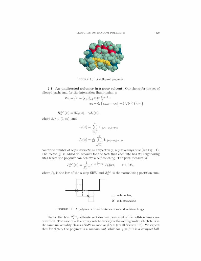
LECTURES ON RANDOM POLYMERS 329
Figure 10. A collapsed polymer.
2.1. An undirected polymer in a poor solvent. Our choice for the set ofallowed paths and for the interaction Hamiltonian is
Wn =w = (wi)
ni=0 ∈ (Zd)n+1 :
w0 = 0, ‖wi+1 − wi‖ = 1 ∀ 0 ≤ i < n,
Hβ,γn (w) = βIn(w)− γJn(w),
where β, γ ∈ (0,∞), and
In(w) =
n∑
i,j=0i<j
1‖wi−wj‖=0,
Jn(w) =12d
n∑
i,j=0
i<j−1
1‖wi−wj‖=1,
count the number of self-intersections, respectively, self-touchings of w (see Fig. 11).The factor 1
2d is added to account for the fact that each site has 2d neighboringsites where the polymer can achieve a self-touching. The path measure is
P β,γn (w) =1
Zβ,γn
e−Hβ,γn (w) Pn(w), w ∈ Wn,
where Pn is the law of the n-step SRW and Zβ,γn is the normalizing partition sum.
self-touching
self-intersection
Figure 11. A polymer with self-intersections and self-touchings.
Under the law P β,γn , self-intersections are penalized while self-touchings arerewarded. The case γ = 0 corresponds to weakly self-avoiding walk, which falls inthe same universality class as SAW as soon as β > 0 (recall Section 1.8). We expectthat for β ≫ γ the polymer is a random coil, while for γ ≫ β it is a compact ball.
330 CARAVENNA, DEN HOLLANDER, AND PETRELIS
A crossover is expected to occur when β and γ are comparable. In the next twosections we identify two phase transition curves.
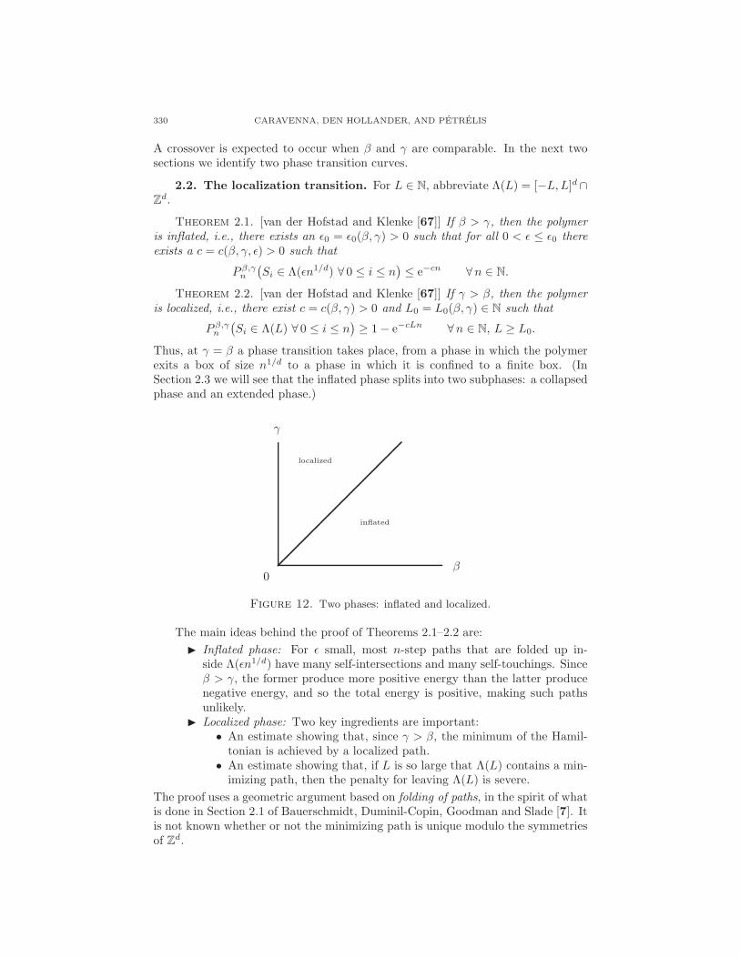
2.2. The localization transition. For L ∈ N, abbreviate Λ(L) = [−L,L]d∩Zd.
Theorem 2.1. [van der Hofstad and Klenke [67]] If β > γ, then the polymeris inflated, i.e., there exists an ǫ0 = ǫ0(β, γ) > 0 such that for all 0 < ǫ ≤ ǫ0 thereexists a c = c(β, γ, ǫ) > 0 such that
P β,γn
(Si ∈ Λ(ǫn1/d) ∀ 0 ≤ i ≤ n
)≤ e−cn ∀n ∈ N.
Theorem 2.2. [van der Hofstad and Klenke [67]] If γ > β, then the polymeris localized, i.e., there exist c = c(β, γ) > 0 and L0 = L0(β, γ) ∈ N such that
P β,γn
(Si ∈ Λ(L) ∀ 0 ≤ i ≤ n
)≥ 1− e−cLn ∀n ∈ N, L ≥ L0.
Thus, at γ = β a phase transition takes place, from a phase in which the polymerexits a box of size n1/d to a phase in which it is confined to a finite box. (InSection 2.3 we will see that the inflated phase splits into two subphases: a collapsedphase and an extended phase.)
0β
γ
inflated
localized
Figure 12. Two phases: inflated and localized.
The main ideas behind the proof of Theorems 2.1–2.2 are:
Inflated phase: For ǫ small, most n-step paths that are folded up in-side Λ(ǫn1/d) have many self-intersections and many self-touchings. Sinceβ > γ, the former produce more positive energy than the latter producenegative energy, and so the total energy is positive, making such pathsunlikely.
Localized phase: Two key ingredients are important:• An estimate showing that, since γ > β, the minimum of the Hamil-tonian is achieved by a localized path.
• An estimate showing that, if L is so large that Λ(L) contains a min-imizing path, then the penalty for leaving Λ(L) is severe.
The proof uses a geometric argument based on folding of paths, in the spirit of whatis done in Section 2.1 of Bauerschmidt, Duminil-Copin, Goodman and Slade [7]. Itis not known whether or not the minimizing path is unique modulo the symmetriesof Zd.
LECTURES ON RANDOM POLYMERS 331
In terms of the mean-square displacement it is predicted that
Eβ,γn (‖Sn‖2) ≍ n2ν as n→ ∞,
where ≍ stands for “asymptotially the same modulo logarithmic factors” (i.e.,Eβ,γn (‖Sn‖2) = n2ν+o(1)). Theorems 2.1–2.2 show that ν = 0 in the localizedphase and ν ≥ 1/d in the inflated phase. It is conjectured in van der Hofstad andKlenke [67] that on the critical line γ = β,
ν = νloc = 1/(d+ 1).
For d = 1, this conjecture is proven in van der Hofstad, Klenke and Konig [68].For d ≥ 2 it is still open. The key simplification that can be exploited when β = γis the relation
In(w) − Jn(w) = −n+ 1
2+
1
8d
∑
x,y∈Zd×Zd
|ℓn(x)− ℓn(y)|2,
where the sum runs over all unordered pairs of neighboring sites, and ℓn(x) =∑ni=0 1wi=x is the local time of w at site x. Since the factor −n+1
2 can be absorbedinto the partition sum, the model at β = γ effectively becomes a model where theenergy is β/4d times the sum of the squares of the gradients of the local times.
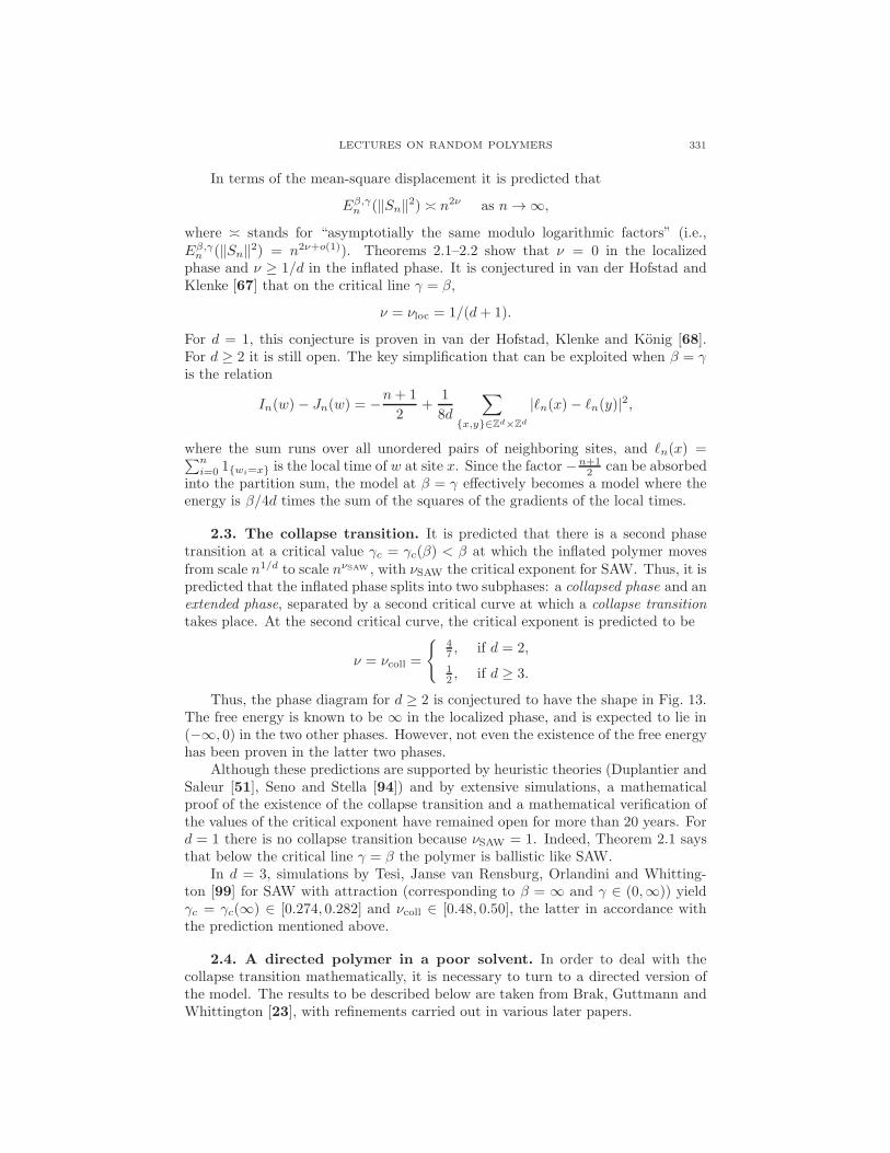
2.3. The collapse transition. It is predicted that there is a second phasetransition at a critical value γc = γc(β) < β at which the inflated polymer movesfrom scale n1/d to scale nνSAW , with νSAW the critical exponent for SAW. Thus, it ispredicted that the inflated phase splits into two subphases: a collapsed phase and anextended phase, separated by a second critical curve at which a collapse transitiontakes place. At the second critical curve, the critical exponent is predicted to be
ν = νcoll =
47 , if d = 2,
12 , if d ≥ 3.
Thus, the phase diagram for d ≥ 2 is conjectured to have the shape in Fig. 13.The free energy is known to be ∞ in the localized phase, and is expected to lie in(−∞, 0) in the two other phases. However, not even the existence of the free energyhas been proven in the latter two phases.
Although these predictions are supported by heuristic theories (Duplantier andSaleur [51], Seno and Stella [94]) and by extensive simulations, a mathematicalproof of the existence of the collapse transition and a mathematical verification ofthe values of the critical exponent have remained open for more than 20 years. Ford = 1 there is no collapse transition because νSAW = 1. Indeed, Theorem 2.1 saysthat below the critical line γ = β the polymer is ballistic like SAW.
In d = 3, simulations by Tesi, Janse van Rensburg, Orlandini and Whitting-ton [99] for SAW with attraction (corresponding to β = ∞ and γ ∈ (0,∞)) yieldγc = γc(∞) ∈ [0.274, 0.282] and νcoll ∈ [0.48, 0.50], the latter in accordance withthe prediction mentioned above.
2.4. A directed polymer in a poor solvent. In order to deal with thecollapse transition mathematically, it is necessary to turn to a directed version ofthe model. The results to be described below are taken from Brak, Guttmann andWhittington [23], with refinements carried out in various later papers.
332 CARAVENNA, DEN HOLLANDER, AND PETRELIS
0 β
γ
γc
ν = 0localized
ν = 1d
collapsed
ν = νloc =1d+1
ν = νcoll
ν = νSAW
extended
Figure 13. Conjectured phase diagram.
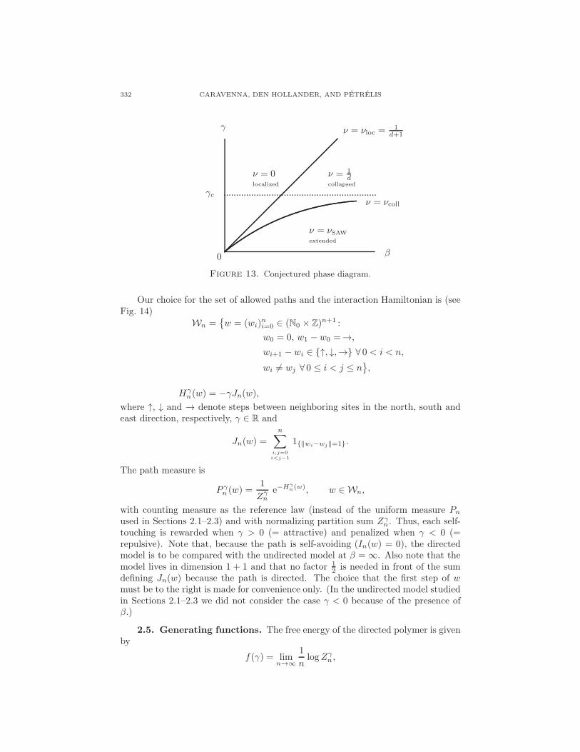
Our choice for the set of allowed paths and the interaction Hamiltonian is (seeFig. 14)
Wn =w = (wi)
ni=0 ∈ (N0 × Z)n+1 :
w0 = 0, w1 − w0 =→,
wi+1 − wi ∈ ↑, ↓,→ ∀ 0 < i < n,
wi 6= wj ∀ 0 ≤ i < j ≤ n,
Hγn(w) = −γJn(w),
where ↑, ↓ and → denote steps between neighboring sites in the north, south andeast direction, respectively, γ ∈ R and
Jn(w) =
n∑
i,j=0i<j−1
1‖wi−wj‖=1.
The path measure is
P γn (w) =1
Zγne−H
γn(w), w ∈ Wn,
with counting measure as the reference law (instead of the uniform measure Pnused in Sections 2.1–2.3) and with normalizing partition sum Zγn . Thus, each self-touching is rewarded when γ > 0 (= attractive) and penalized when γ < 0 (=repulsive). Note that, because the path is self-avoiding (In(w) = 0), the directedmodel is to be compared with the undirected model at β = ∞. Also note that themodel lives in dimension 1 + 1 and that no factor 1
2 is needed in front of the sumdefining Jn(w) because the path is directed. The choice that the first step of wmust be to the right is made for convenience only. (In the undirected model studiedin Sections 2.1–2.3 we did not consider the case γ < 0 because of the presence ofβ.)
2.5. Generating functions. The free energy of the directed polymer is givenby
f(γ) = limn→∞
1
nlogZγn ,
LECTURES ON RANDOM POLYMERS 333
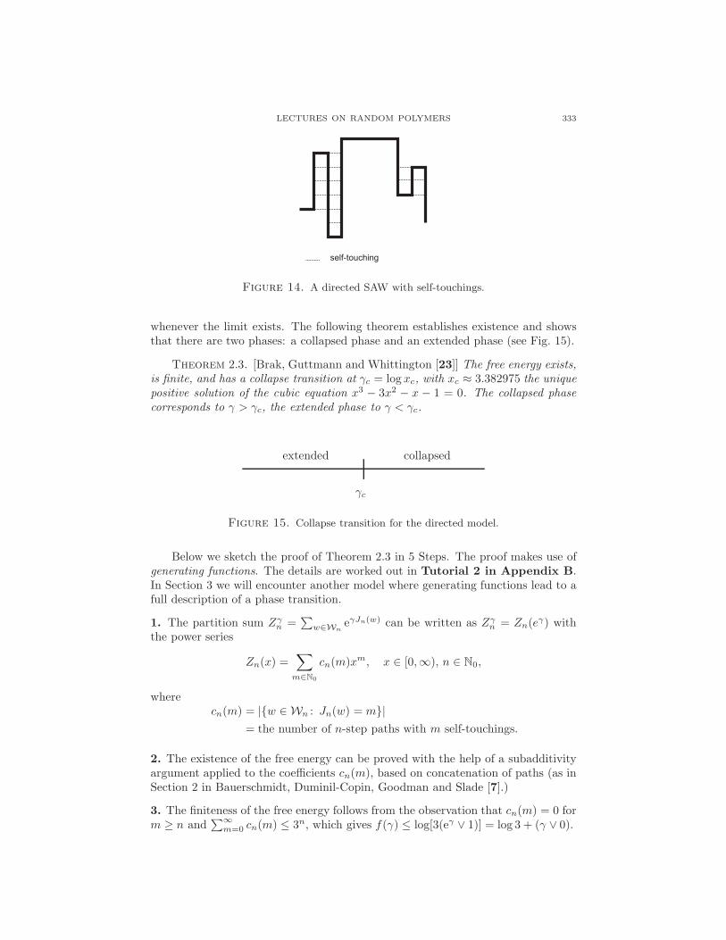
self-touching
Figure 14. A directed SAW with self-touchings.
whenever the limit exists. The following theorem establishes existence and showsthat there are two phases: a collapsed phase and an extended phase (see Fig. 15).
Theorem 2.3. [Brak, Guttmann and Whittington [23]] The free energy exists,is finite, and has a collapse transition at γc = log xc, with xc ≈ 3.382975 the uniquepositive solution of the cubic equation x3 − 3x2 − x − 1 = 0. The collapsed phasecorresponds to γ > γc, the extended phase to γ < γc.
γc
extended collapsed
Figure 15. Collapse transition for the directed model.
Below we sketch the proof of Theorem 2.3 in 5 Steps. The proof makes use ofgenerating functions. The details are worked out in Tutorial 2 in Appendix B.In Section 3 we will encounter another model where generating functions lead to afull description of a phase transition.
1. The partition sum Zγn =∑
w∈WneγJn(w) can be written as Zγn = Zn(e
γ) withthe power series
Zn(x) =∑
m∈N0
cn(m)xm, x ∈ [0,∞), n ∈ N0,
wherecn(m) = |w ∈ Wn : Jn(w) = m|
= the number of n-step paths with m self-touchings.
2. The existence of the free energy can be proved with the help of a subadditivityargument applied to the coefficients cn(m), based on concatenation of paths (as inSection 2 in Bauerschmidt, Duminil-Copin, Goodman and Slade [7].)
3. The finiteness of the free energy follows from the observation that cn(m) = 0 form ≥ n and
∑∞m=0 cn(m) ≤ 3n, which gives f(γ) ≤ log[3(eγ ∨ 1)] = log 3 + (γ ∨ 0).

334 CARAVENNA, DEN HOLLANDER, AND PETRELIS
4. The following lemma gives a closed form expression for the generating function(x = eγ)
G = G(x, y) =∑
n∈N0
Zn(x) yn
=∑
n∈N0
[ n∑
m=0
cn(m)xm]yn, x, y ∈ [0,∞).
Lemma 2.4. For x, y ∈ [0,∞) the generating function is given by the formalpower series
G(x, y) = −aH(x, y)− 2y2
bH(x, y)− 2y2,
where
a = y2(2 + y − xy), b = y2(1 + x+ y − xy), H(x, y) = yg0(x, y)
g1(x, y),
with
gr(x, y) = yr
(1 +
∑
k∈N
(y − q)k y2k q12k(k+1)
∏kl=1(yq
l − y)(yql − q)qkr
),
q = xy, r = 0, 1.
The function H(x, y) is a quotient of two q-hypergeometric functions (which aresingular at least along the curve q = xy = 1). As shown in Brak, Guttmann andWhittington [23], the latter can be expressed as continued fractions and thereforecan be properly analyzed (as well as computed numerically).
xc0x
yc(x)
Figure 16. The domain of convergence of the generating functionG(x, y) lies below the critical curve (= solid curve). The dotted lineis the hyperbola xy = 1 (corresponding to q = 1). The point xc isidentified with the collapse transition, because this is where the freeenergy is non-analytic.
5. By analyzing the singularity structure of G(x, y) it is possible to compute f(γ).Indeed, the task is to identify the critical curve x 7→ yc(x) in the (x, y)-plane belowwhich G(x, y) has no singularities and on or above which it does, because thisidentifies the free energy as
f(γ) = − log yc(eγ), γ ∈ R.
LECTURES ON RANDOM POLYMERS 335
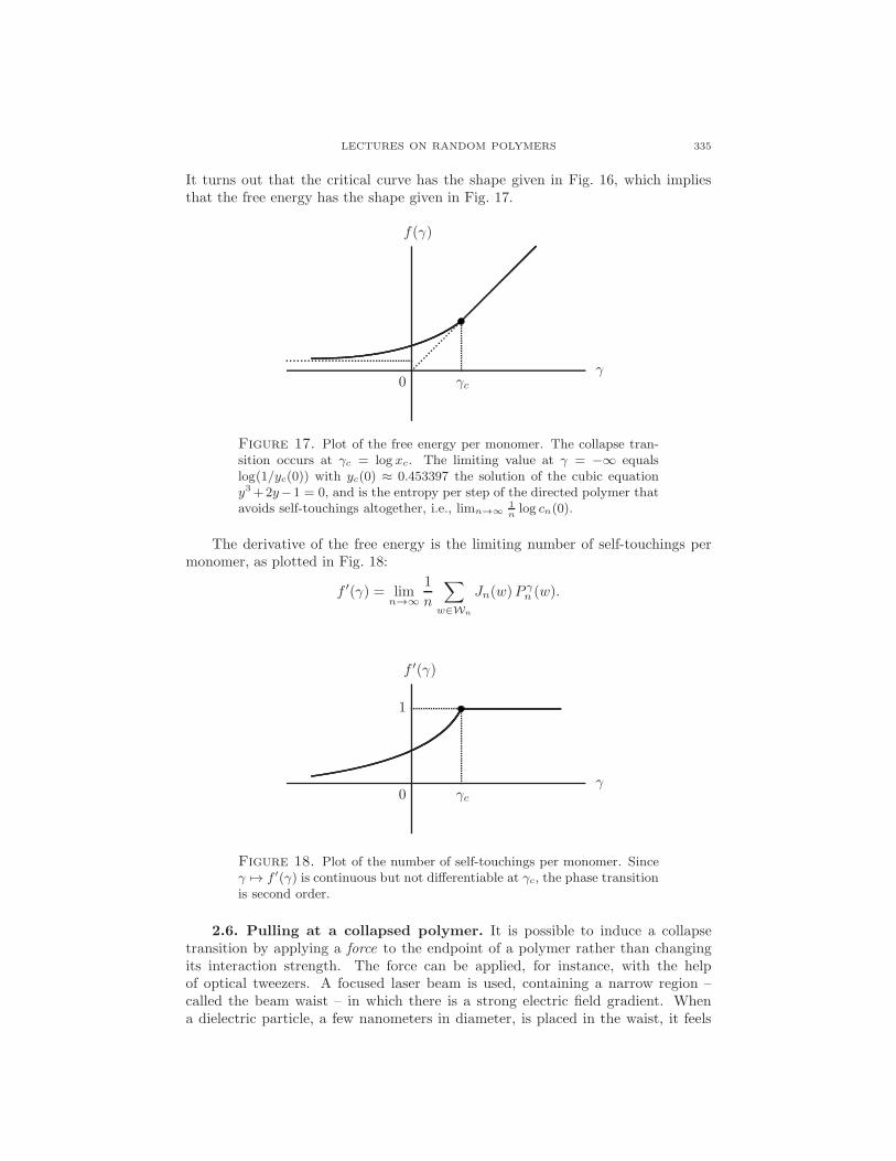
It turns out that the critical curve has the shape given in Fig. 16, which impliesthat the free energy has the shape given in Fig. 17.
γc0γ
f(γ)
Figure 17. Plot of the free energy per monomer. The collapse tran-sition occurs at γc = log xc. The limiting value at γ = −∞ equalslog(1/yc(0)) with yc(0) ≈ 0.453397 the solution of the cubic equationy3+2y−1 = 0, and is the entropy per step of the directed polymer thatavoids self-touchings altogether, i.e., limn→∞
1nlog cn(0).
The derivative of the free energy is the limiting number of self-touchings permonomer, as plotted in Fig. 18:
f ′(γ) = limn→∞
1
n
∑
w∈Wn
Jn(w)Pγn (w).
γc
1
0γ
f ′(γ)
Figure 18. Plot of the number of self-touchings per monomer. Sinceγ 7→ f ′(γ) is continuous but not differentiable at γc, the phase transitionis second order.
2.6. Pulling at a collapsed polymer. It is possible to induce a collapsetransition by applying a force to the endpoint of a polymer rather than changingits interaction strength. The force can be applied, for instance, with the helpof optical tweezers. A focused laser beam is used, containing a narrow region –called the beam waist – in which there is a strong electric field gradient. Whena dielectric particle, a few nanometers in diameter, is placed in the waist, it feels
336 CARAVENNA, DEN HOLLANDER, AND PETRELIS
a strong attraction towards the center of the waist. It is possible to chemicallyattach such a particle to the end of the polymer and then pull on the particle withthe laser beam, thereby effectively exerting a force on the polymer itself. Currentexperiments allow for forces in the range of 10−12 − 10−15 Newton. With suchmicroscopically small forces the structural, mechanical and elastic properties ofpolymers can be probed. We refer to Auvray, Duplantier, Echard and Sykes [6],Section 5.2, for more details. The force is the result of transversal fluctuations ofthe dielectric particle, which can be measured with great accuracy.
Ioffe and Velenik [77, 78, 79, 80] consider a version of the undirected modelin which the Hamiltonian takes the form
Hψ,φn (w) =
∑
x∈Zd
ψ(ℓn(x)
)− (φ,wn), w ∈ Wn,
where Wn is the set of allowed n-step paths for the undirected model consideredin Sections 2.1–2.3, ℓn(x) =
∑ni=0 1wi=x is the local time of w at site x ∈ Z
d,
ψ : N0 → [0,∞) is non-decreasing with ψ(0) = 0, and φ ∈ Rd is a force acting on
the endpoint of the polymer. Note that (φ,wn) is the work exerted by the force φto move the endpoint of the polymer to wn. The path measure is
Pψ,φn (w) =1
Zψ,φn
e−Hψ,φn (w) Pn(w), w ∈ Wn,
with Pn the law of SRW.Two cases are considered:
(1) ψ is superlinear (= repulsive interaction).(2) ψ is sublinear with limℓ→∞ ψ(ℓ)/ℓ = 0 (= attractive interaction).
Typical examples are:
(1) ψ(ℓ) = βℓ2 (which corresponds to the weakly self-avoiding walk).
(2) ψ(ℓ) =∑ℓ
k=1 βk with k 7→ βk non-increasing such that limk→∞ βk = 0(which corresponds to the annealed version of the model of a polymer in arandom potential described in Section 6, for the case where the potentialis non-negative).
It is shown in Ioffe and Velenik [77, 78, 79, 80] (see also references cited therein)that:
(1) The polymer is in an extended phase for all φ ∈ Rd.
(2) There is a compact convex set K = K(ψ) ⊂ Rd, with int(K) ∋ 0, such
that the polymer is in a collapsed phase (= subballistic) when φ ∈ int(K)and in an extended phase (= ballistic) when φ /∈ K.
The proof uses coarse-graining arguments, showing that in the extended phase largesegments of the polymer can be treated as directed. For d ≥ 2, the precise shapeof the set K is not known. It is known that K has the symmetries of Zd and has alocally analytic boundary ∂K with a uniformly positive Gaussian curvature. It ispredicted not to be a ball, but this has not been proven. The phase transition at∂K is first order.
2.7. Open problems. The main challenges are:
• Prove the conjectured phase diagram in Fig. 13 for the undirected (β, γ)-model studied Sections 2.1–2.3 and determine the order of the phase tran-sitions.
LECTURES ON RANDOM POLYMERS 337
• Extend the analysis of the directed γ-model studied in Sections 2.4–2.5 to1 + d dimensions with d ≥ 2.
• Find a closed form expression for the set K of the undirected ψ-modelstudied in Section 2.6.
For the undirected model in d = 2, the scaling limit is predicted to be:
(1) SLE8 in the collapsed phase (between the two critical curves),(2) SLE6 at the collapse transition (on the lower critical curve),(3) SLE8/3 in the extended phase (below the lower critical curve),
all three with a time parametrization that depends on β and γ (see the lectures byBeffara [8] for an explanation of the time parametrization). Case (1) is plausiblebecause SLE8 is space filling, while we saw in Section 2.2 that the polymer rolls itselfup inside a ball with a volume equal to the polymer length. Case (2) is plausiblebecause on the hexagonal lattice the exploration process in critical percolation has apath measure that, apart from higher order terms, is equal to that of the SAW witha critical reward for self-touchings (numerical simulation shows that γc ≈ log 2.8),and this exploration process has been proven to scale to SLE6 (discussions withVincent Beffara and Markus Heydenreich). Case (3) is plausible because SLE8/3 ispredicted to be the scaling limit of SAW (see Section 1.7).
3. A polymer near a homogeneous interface
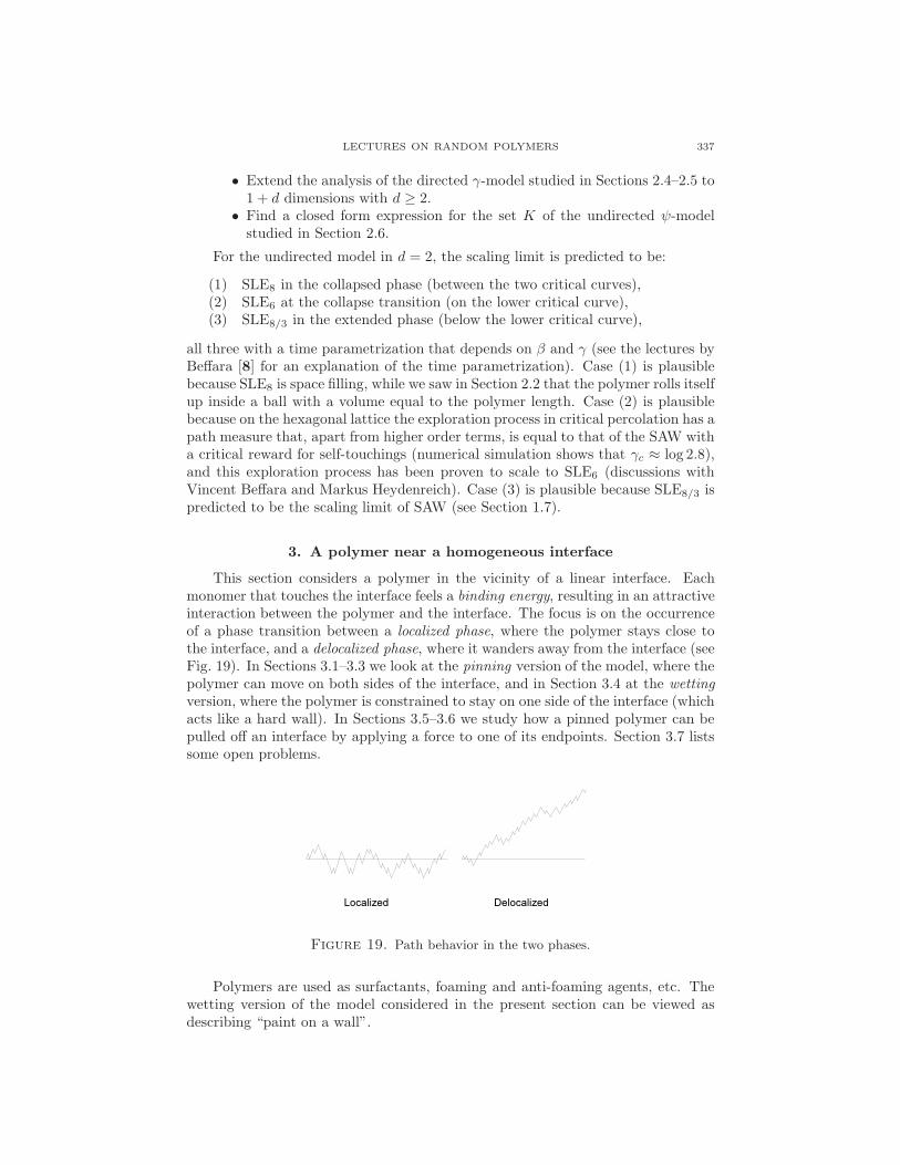
This section considers a polymer in the vicinity of a linear interface. Eachmonomer that touches the interface feels a binding energy, resulting in an attractiveinteraction between the polymer and the interface. The focus is on the occurrenceof a phase transition between a localized phase, where the polymer stays close tothe interface, and a delocalized phase, where it wanders away from the interface (seeFig. 19). In Sections 3.1–3.3 we look at the pinning version of the model, where thepolymer can move on both sides of the interface, and in Section 3.4 at the wettingversion, where the polymer is constrained to stay on one side of the interface (whichacts like a hard wall). In Sections 3.5–3.6 we study how a pinned polymer can bepulled off an interface by applying a force to one of its endpoints. Section 3.7 listssome open problems.
Figure 19. Path behavior in the two phases.
Polymers are used as surfactants, foaming and anti-foaming agents, etc. Thewetting version of the model considered in the present section can be viewed asdescribing “paint on a wall”.

338 CARAVENNA, DEN HOLLANDER, AND PETRELIS
3.1. Model. Our choices for the set of paths and for the interaction Hamil-tonian are
Wn =w = (i, wi)
ni=0 : w0 = 0, wi ∈ Z ∀ 0 ≤ i ≤ n
,
Hζn(w) = −ζLn(w),
with ζ ∈ R and
Ln(w) =
n∑
i=1
1wi=0, w ∈ Wn,
the local time of w at the interface. The path measure is
P ζn(w) =1
Zζne−H
ζn(w) Pn(w), w ∈ Wn,
where Pn is the projection onto Wn of the path measure P of an arbitrary directedirreducible random walk. This models a (1 + 1)-dimensional directed polymer inN0×Z in which each visit to the interface N×0 contributes an energy −ζ, whichis a reward when ζ > 0 and a penalty when ζ < 0 (see Fig. 20).
N× 0(0, 0)
Figure 20. A 7-step two-sided path that makes 2 visits to the interface.
Let S = (Si)i∈N0denote the random walk with law P starting from S0 = 0.
LetR(n) = P (Si 6= 0 ∀ 1 ≤ i < n, Sn = 0), n ∈ N.
denote the return time distribution to the interface. Throughout the sequel it isassumed that
∑n∈N
R(n) = 1 and
R(n) = n−1−a ℓ(n), n ∈ N,
for some a ∈ (0,∞) and some ℓ(·) slowly varying at infinity (i.e., limx→∞ ℓ(cx)/ℓ(x)= 1 for all c ∈ (0,∞)). Note that this assumption implies that R(n) > 0 for n largeenough, i.e., R(·) is aperiodic. It is trivial, however, to extend the analysis belowto include the periodic case. SRW corresponds to a = 1
2 and period 2.
3.2. Free energy. The free energy can be computed explicitly. Let φ(x) =∑n∈N
xnR(n), x ∈ [0,∞).
Theorem 3.1. [Fisher [53], Giacomin [55], Chapter 2] The free energy
f(ζ) = limn→∞
1
nlogZζn
exists for all ζ ∈ R and is given by
f(ζ) =
0, if ζ ≤ 0,r(ζ), if ζ > 0,
where r(ζ) is the unique solution of the equation
φ(e−r) = e−ζ, ζ > 0.
LECTURES ON RANDOM POLYMERS 339
Proof. For ζ ≤ 0, estimate
∑
m>n
R(m) = P (Si 6= 0 ∀ 1 ≤ i ≤ n) ≤ Zζn ≤ 1,
which implies f(ζ) = 0 because the left-hand side decays polynomially in n.For ζ > 0, let
Rζ(n) = eζ−r(ζ)nR(n), n ∈ N.
By the definition of r(ζ), this is a probability distribution on N, with a finite meanM ζ =
∑n∈N
nRζ(n) because r(ζ) > 0. The partition sum when the polymer isconstrained to end at 0 can be written as
Z∗,ζn =
∑
w∈Wnwn=0
eζLn(w) Pn(w) = er(ζ)nQζ(n ∈ T )
with
Qζ(n ∈ T ) =
n∑
m=1
∑
j1,...,jm∈N
j1+···+jm=n
m∏
k=1
Rζ(jk),
where T is the renewal process whose law Qζ is such that the i.i.d. renewals havelaw Rζ. Therefore, by the renewal theorem,
limn→∞
Qζ(n ∈ T ) = 1/M ζ,
which yields
limn→∞
1
nlogZ∗,ζ
n = r(ζ).
By splitting the partition sum Zζn according to the last hitting time of 0 (seethe end of Tutorial 1 in Appendix A), it is straightforward to show that thereexists a C <∞ such that
Z∗,ζn ≤ Zζn ≤ (1 + Cn)Z∗,ζ
n ∀n ∈ N0.
It therefore follows that
f(ζ) = limn→∞
1
nlogZζn = r(ζ).
For SRW (see Spitzer [97], Section 1)
φ(x) = 1−√1− x2, x ∈ [0, 1].
By Theorem 3.1, this gives
f(ζ) = r(ζ) = 12
[ζ − log(2− e−ζ)
], f ′(ζ) = 1
2
[1− e−ζ
2−e−ζ
], ζ > 0,
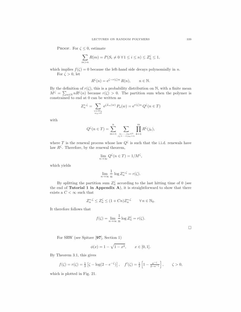
which is plotted in Fig. 21.
340 CARAVENNA, DEN HOLLANDER, AND PETRELIS
0ζ
f(ζ)12 ζ − 1
2 log 2
Figure 21. Plot of the free energy for pinned SRW.
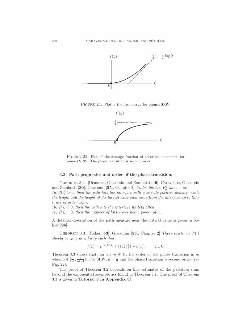
12
0ζ
f ′(ζ)
Figure 22. Plot of the average fraction of adsorbed monomers forpinned SRW. The phase transition is second order.
3.3. Path properties and order of the phase transition.
Theorem 3.2. [Deuschel, Giacomin and Zambotti [49], Caravenna, Giacominand Zambotti [30], Giacomin [55], Chapter 2] Under the law P ζn as n→ ∞:(a) If ζ > 0, then the path hits the interface with a strictly positive density, whilethe length and the height of the largest excursion away from the interface up to timen are of order logn.(b) If ζ < 0, then the path hits the interface finitely often.(c) If ζ = 0, then the number of hits grows like a power of n.
A detailed description of the path measure near the critical value is given in So-hier [96].
Theorem 3.3. [Fisher [53], Giacomin [55], Chapter 2] There exists an ℓ∗(·)slowly varying at infinity such that
f(ζ) = ζ1/(1∧a) ℓ∗(1/ζ) [1 + o(1)], ζ ↓ 0.
Theorem 3.3 shows that, for all m ∈ N, the order of the phase transition is mwhen a ∈ [ 1m ,
1m−1). For SRW, a = 1
2 and the phase transition is second order (see
Fig. 22).The proof of Theorem 3.2 depends on fine estimates of the partition sum,
beyond the exponential asymptotics found in Theorem 3.1. The proof of Theorem3.3 is given in Tutorial 3 in Appendix C.

LECTURES ON RANDOM POLYMERS 341
3.4. Wetting. What happens when the interface is impenetrable? Then theset of paths is replaced by (see Fig. 23)
W+n =
w = (i, wi)
ni=0 : w0 = 0, wi ∈ N0 ∀ 0 ≤ i ≤ n
.
Accordingly, write P ζ,+n (w), Zζ,+n and f+(ζ) for the path measure, the partitionsum and the free energy. One-sided pinning at an interface is called wetting.
N× 0(0, 0)
Figure 23. A 7-step one-sided path that makes 2 visits to the interface.
Let
R+(n) = P (Si > 0 ∀ 1 ≤ i < n, Sn = 0), n ∈ N.
This is a defective probability distribution. Define
φ+(x) =∑
n∈N
xnR+(n), x ∈ [0,∞),
and put
φ(x) =φ+(x)
φ+(1), ζ+c = log
[ 1
φ+(1)
]> 0.
Theorem 3.4. [Fisher [53], Giacomin [55], Chapter 2] The free energy is givenby
f+(ζ) =
0, if ζ ≤ ζ+c ,r+(ζ), if ζ > ζ+c ,
where r+(ζ) is the unique solution of the equation
φ(e−r) = e−(ζ−ζ+c ), ζ > ζ+c .
The proof is similar to that of the pinned polymer. Localization on an im-penetrable interface is harder than on a penetrable interface, because the polymersuffers a larger loss of entropy. This is the reason why ζ+c > 0. For SRW, symmetrygives
R+(n) = 12 R(n), n ∈ N.
Consequently,
ζ+c = log 2, φ(·) = φ(·),implying that
f+(ζ) = f(ζ − ζ+c ), ζ ∈ R.
Thus, the free energy suffers a shift (i.e., the curves in Figs. 21–22 move to the rightby log 2) and the qualitative behavior is similar to that of pinning.
342 CARAVENNA, DEN HOLLANDER, AND PETRELIS
3.5. Pulling at an adsorbed polymer. A polymer can be pulled off aninterface by a force. Replace the pinning Hamiltonian by
Hζ,φn (w) = −ζLn(w) − φwn,
where φ ∈ (0,∞) is a force in the upward direction acting on the endpoint of thepolymer. Note that φwn is the work exerted by the force to move the endpoint adistance wn away from the interface. Write Zζ,φn to denote the partition sum and
f(ζ, φ) = limn→∞
1
nlogZζ,φn
to denote the free energy. Consider the case where the reference random walk canonly make steps of size ≤ 1, i.e., pick p ∈ [0, 1] and put
P (S1 = −1) = P (S1 = +1) = 12p, P (S1 = 0) = 1− p.
Theorem 3.5. [Giacomin and Toninelli [62]] For every ζ ∈ R and φ > 0, thefree energy exists and is given by
f(ζ, φ) = f(ζ) ∨ g(φ),with f(ζ) the free energy of the pinned polymer without force and
g(φ) = log[p cosh(φ) + (1− p)
].
Proof. Write
Zζ,φn = Z∗,ζn +
n∑
m=1
Z∗,ζn−m Z
φm,
where Z∗,ζn is the constrained partition sum without force encountered in Sec-
tions 3.1–3.3, and
Zφm =∑
x∈Z\0
eφxR(m;x), m ∈ N,
with
R(m;x) = P(Si 6= 0 ∀ 1 ≤ i < m, Sm = x
).
It suffices to show that
g(φ) = limm→∞
1
mlog Zφm,
which will yield the claim because
f(ζ) = limn→∞
1
nlogZ∗,ζ
n .
The contribution to Zφm coming from x ∈ Z\N0 is bounded from above by1/(1 − e−φ) < ∞ and therefore is negligible. (The polymer does not care to staybelow the interface because the force is pulling it upwards.) For x ∈ N the reflectionprinciple gives
R(m;x) = 12pP
(Si > 0 ∀ 2 ≤ i < m, Sm = x | S1 = 1
)
= 12p[P (Sm = x | S1 = 1)− P (Sm = x | S1 = −1)
]
= 12p[P (Sm−1 = x− 1)− P (Sm−1 = x+ 1)
]∀m ∈ N.
The first equality holds because the path cannot jump over the interface. Thesecond inequality holds because, for any path from 1 to x that hits the interface,the piece of the path until the first hit of the interface can be reflected in the
LECTURES ON RANDOM POLYMERS 343
interface to yield a path from −1 to x. Substitution of the above relation into thesum defining Zφm gives
Zφm = O(1) + p sinh(φ)∑
x∈N
eφx P (Sm−1 = x)
= O(1) +O(1) + p sinh(φ)E(eφSm−1
).
ButE(eφSm−1
)= [p cosh(φ) + (1 − p)]m−1,
and so the above claim follows.
The force either leaves most of the polymer adsorbed, when
f(ζ, φ) = f(ζ) > g(φ),
or pulls most of the polymer off, when
f(ζ, φ) = g(φ) > f(ζ).
A first-order phase transition occurs at those values of ζ and φ where f(ζ) = g(φ),i.e., the critical value of the force is given by
φc(ζ) = g−1(f(ζ)
), ζ ∈ R,
with g−1 the inverse of g. Think of g(φ) as the free energy of the polymer withforce φ not interacting with the interface.
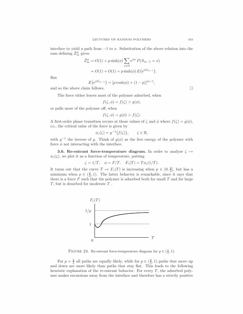
3.6. Re-entrant force-temperature diagram. In order to analyze ζ 7→φc(ζ), we plot it as a function of temperature, putting
ζ = 1/T, φ = F/T, Fc(T ) = Tφc(1/T ).
It turns out that the curve T 7→ Fc(T ) is increasing when p ∈ (0, 23 ], but has a
minimum when p ∈ (23 , 1). The latter behavior is remarkable, since it says thatthere is a force F such that the polymer is adsorbed both for small T and for largeT , but is desorbed for moderate T .
0T
Fc(T )
1
1/p
Figure 24. Re-entrant force-temperature diagram for p ∈ ( 23, 1).
For p = 23 all paths are equally likely, while for p ∈ (23 , 1) paths that move up
and down are more likely than paths that stay flat. This leads to the followingheuristic explanation of the re-entrant behavior. For every T , the adsorbed poly-mer makes excursions away from the interface and therefore has a strictly positive

344 CARAVENNA, DEN HOLLANDER, AND PETRELIS
entropy. Some of this entropy is lost when a force is applied to the endpoint of thepolymer, so that the part of the polymer near the endpoint is pulled away from theinterface and is caused to move upwards steeply. There are two cases:
p = 23 : As T increases the effect of this entropy loss on the free energy increases,
because “free energy = energy− temperature× entropy”. This effect must be coun-terbalanced by a larger force to achieve desorption.
p ∈ (23 , 1): Steps in the east direction are favored over steps in the north-east andsouth-east directions, and this tends to place the adsorbed polymer farther awayfrom the interface. Hence the force decreases for small T (i.e., Fc(T ) < Fc(0) forsmall T , because at T = 0 the polymer is fully adsorbed).
3.7. Open problems. Some key challenges are:
• Investigate pinning and wetting of SAW by a linear interface, i.e., studythe undirected version of the model in Sections 3.1–3.4. Partial resultshave been obtained in the works of A.J. Guttmann, J. Hammersley, E.J.Janse van Rensburg, E. Orlandini, A. Owczarek, A. Rechnitzer, C. Soteros,C. Tesi, S.G. Whittington, and others. For references, see den Hollan-der [70], Chapter 7.
• Look at polymers living inside wedges or slabs, with interaction at theboundary. This leads to combinatorial problems of the type described inthe lectures by Di Francesco during the summer school, many of whichare hard. There is a large literature, with contributions coming from M.Bousquet-Melou, R. Brak, A.J. Guttmann, E.J. Janse van Rensburg, A.Owczarek, A. Rechnitzer, S.G. Whittington, and others. For references,see Guttmann [64].
• Caravenna and Petrelis [31, 32] study a directed polymer pinned by aperiodic array of interfaces. They identify the rate at which the polymerhops between the interfaces as a function of their mutual distance anddetermine the scaling limit of the endpoint of the polymer. There areseveral regimes depending on the sign of the adsorption strength and onhow the distance between the interfaces scales with the length of thepolymer. Investigate what happens when the interfaces are placed atrandom distances.
• What happens when the shape of the interface itself is random? Pinningof a polymer by a polymer, both performing directed random walks, canbe modelled by the Hamiltonian Hζ
n(w,w′) = −ζLn(w,w′), ζ ∈ R, with
Ln(w,w′) =
∑ni=1 1wi=w′
ithe collision local time of w,w′ ∈ Wn, the
set of directed paths introduced in Section 3.1. This model was studiedby Birkner, Greven and den Hollander [13], Birkner and Sun [14, 15],Berger and Toninelli [9]. A variational formula for the critical adsorptionstrength is derived in [13]. This variational formula turns out to be hardto analyze.
LECTURES ON RANDOM POLYMERS 345
In Sections 1–3 we considered several models of a polymer chain interactingwith itself and/or with an interface. In Sections 4–6 we move to models withdisorder, i.e., there is a random environment with which the polymer chainis interacting. Models with disorder are much harder than models withoutdisorder. In order to advance mathematically, we will restrict ourselves todirected paths.
4. A polymer near a random interface
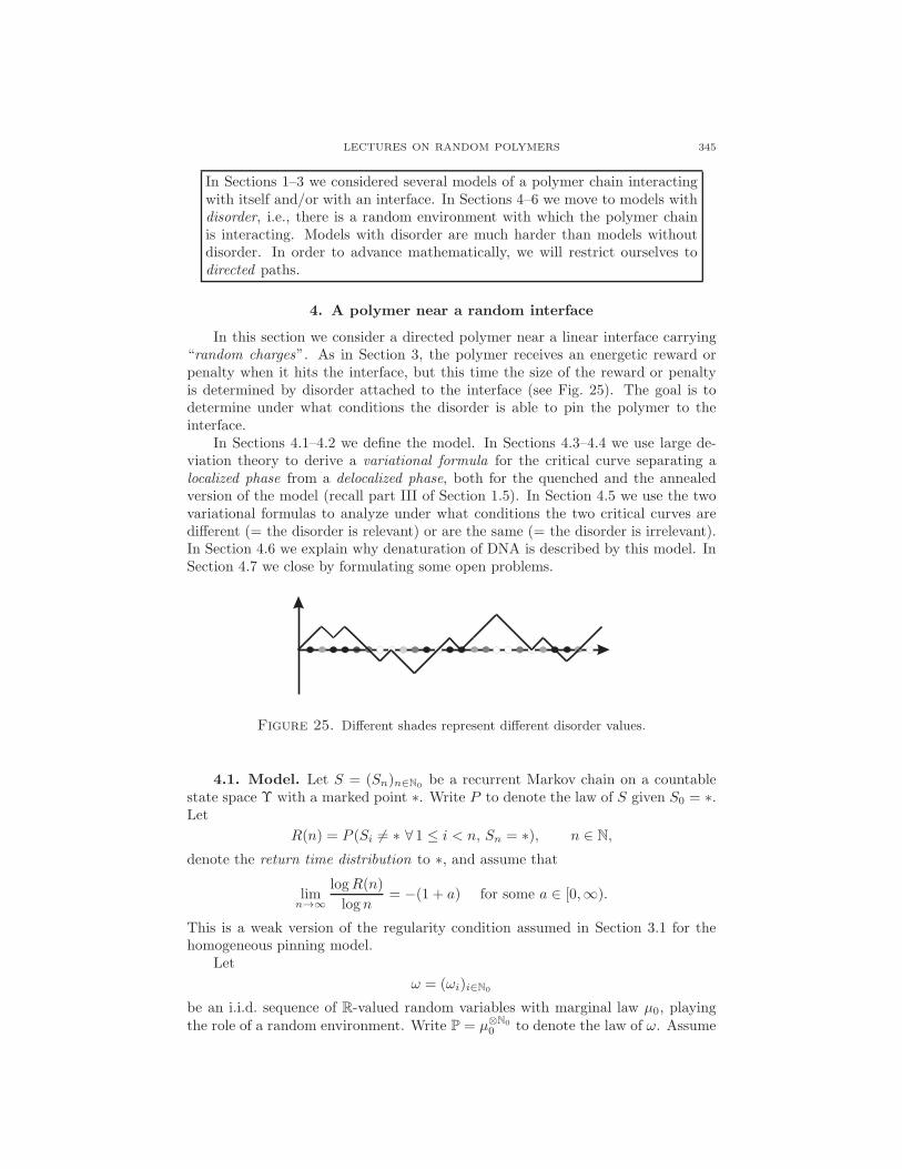
In this section we consider a directed polymer near a linear interface carrying“random charges”. As in Section 3, the polymer receives an energetic reward orpenalty when it hits the interface, but this time the size of the reward or penaltyis determined by disorder attached to the interface (see Fig. 25). The goal is todetermine under what conditions the disorder is able to pin the polymer to theinterface.
In Sections 4.1–4.2 we define the model. In Sections 4.3–4.4 we use large de-viation theory to derive a variational formula for the critical curve separating alocalized phase from a delocalized phase, both for the quenched and the annealedversion of the model (recall part III of Section 1.5). In Section 4.5 we use the twovariational formulas to analyze under what conditions the two critical curves aredifferent (= the disorder is relevant) or are the same (= the disorder is irrelevant).In Section 4.6 we explain why denaturation of DNA is described by this model. InSection 4.7 we close by formulating some open problems.
Figure 25. Different shades represent different disorder values.
4.1. Model. Let S = (Sn)n∈N0be a recurrent Markov chain on a countable
state space Υ with a marked point ∗. Write P to denote the law of S given S0 = ∗.Let
R(n) = P (Si 6= ∗ ∀ 1 ≤ i < n, Sn = ∗), n ∈ N,
denote the return time distribution to ∗, and assume that
limn→∞
logR(n)
logn= −(1 + a) for some a ∈ [0,∞).
This is a weak version of the regularity condition assumed in Section 3.1 for thehomogeneous pinning model.
Let
ω = (ωi)i∈N0
be an i.i.d. sequence of R-valued random variables with marginal law µ0, playingthe role of a random environment. Write P = µ⊗N0
0 to denote the law of ω. Assume
346 CARAVENNA, DEN HOLLANDER, AND PETRELIS
that µ0 is non-degenerate and satisfies
M(β) = E(eβω0) =
∫
R
eβxµ(dx) <∞ ∀β ≥ 0.
For fixed ω, define a law on the set of directed paths of length n ∈ N0 byputting
dP β,h,ωn
dPn
((i, Si)
ni=0
)=
1
Zβ,h,ωn
exp
[n−1∑
i=0
(βωi − h) 1Si=∗
],
where β ∈ [0,∞) is the disorder strength, h ∈ R is the disorder bias, Pn is theprojection of P onto n-step paths, and Zβ,h,ωn is the normalizing partition sum.Note that the homogeneous pinning model in Section 3 is recovered by puttingβ = 0 and h = −ζ (with the minor difference that now the Hamiltonian includesthe term with i = 0 but not the term with i = n). Without loss of generality wecan choose µ0 to be such that E(ω0) = 0, E(ω2
0) = 1 (which amounts to a shift ofthe parameters β, h).
In our standard notation, the above model corresponds to the choice
Wn =w = (i, wi)
ni=0 : w0 = ∗, wi ∈ Υ ∀ 0 < i ≤ n
,
Hβ,h,ωn (w) = −
n−1∑
i=0
(βωi − h) 1wi=∗.
(As before, we think of (Si)ni=0 as the realization of (wi)
ni=0 drawn according to
P β,h,ωn .) The key example modelling our polymer with pinning is
Υ = Zd, ∗ = 0, P = law of directed SRW in Z
d, d = 1, 2,
for which a = 12 and a = 0, respectively. We expect that pinning occurs for large β
and/or small h: the polymer gets a large enough energetic reward when it hits thepositive charges and does not lose too much in terms of entropy when it avoids thenegative charges. For the same reason we expect that no pinning occurs for smallβ and/or large h. In Sections 4.2–4.6 we identify the phase transition curve andinvestigate its properties.
4.2. Free energies. The quenched free energy is defined as
fque(β, h) = limn→∞
1
nlogZβ,h,ωn ω−a.s.
Subadditivity arguments show that ω-a.s. the limit exists and is non-random (seeTutorial 1 in Appendix A). Since
Zβ,h,ωn = E
(exp
[n−1∑
i=0
(βωi − h) 1Si=∗
])≥ eβω0−h
∑
m≥n
R(m),
which decays polynomially in n, it follows that fque(β, h) ≥ 0. This fact motivatesthe definition
L =(β, h) : fque(β, h) > 0
,
D =(β, h) : fque(β, h) = 0
,
which are referred to as the quenched localized phase, respectively, the quencheddelocalized phase. The associated quenched critical curve is
hquec (β) = infh ∈ R : fque(β, h) = 0, β ∈ [0,∞).
LECTURES ON RANDOM POLYMERS 347
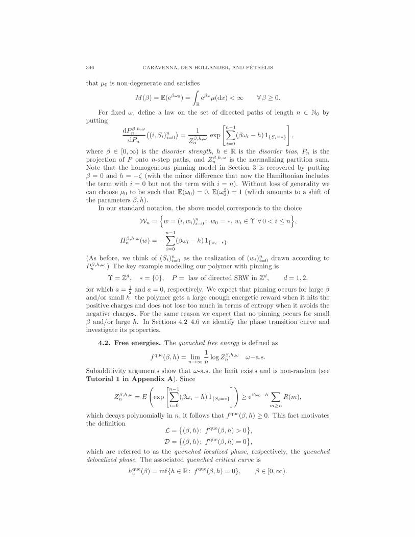
Because h 7→ fque(β, h) is non-increasing, we have fque(β, h) = 0 for h ≥ hquec (β).Convexity of (β, h) 7→ fque(β, h) implies that β 7→ hquec (β) is convex. It is easyto check that both are finite (this uses the bound fque ≤ fann with fann theannealed free energy defined below) and therefore are also continuous. Futhermore,hquec (0) = 0 (because the critical threshold for the homogeneous pinning model iszero), and hquec (β) > 0 for β > 0 (see below). Together with convexity the latterimply that β 7→ hquec (β) is strictly increasing.
Alexander and Sidoravicius [3] prove that hquec (β) > 0 for β > 0 for arbitrarynon-degenerate µ0 (see Fig. 26). This result is important, because it shows thatlocalization occurs even for a moderately negative average value of the disorder,contrary to what we found for the homogeneous pinning model in Section 3. Indeed,since E(βω1 − h) = −h < 0, even a globally repulsive interface can locally pin thepolymer provided the global repulsion is modest: all the polymer has to do is hitthe positive charges and avoid the negative charges.
0β
h
LD
Figure 26. Qualitative picture of β 7→ hquec (β) (the asymptote has
finite slope if and only if the support of µ0 is bounded from above). Thedetails of the curve are known only partially (see below).
The annealed free energy is defined by (recall Section 1.5)
fann(β, h) = limn→∞
1
nlogE
(Zβ,h,ωn
).
This is the free energy of a homopolymer. Indeed, E(Zβ,h,ωn ) = Zh−logM(β)n , the
partition function of the homogeneous pinning model with parameter h− logM(β).The associated annealed critical curve
hannc (β) = infh ∈ R : fann(β, h) = 0, β ∈ [0,∞),
can therefore be computed explicitly:
hannc (β) = logE(eβω0) = logM(β).
By Jensen’s inequality, we have
fque ≤ fann −→ hquec ≤ hannc .
In Fig. 28 below we will see how the two critical curves are related.
Definition 4.1. For a given choice of R, µ0 and β, the disorder is said to berelevant when hquec (β) < hannc (β) and irrelevant when hquec (β) = hannc (β).
348 CARAVENNA, DEN HOLLANDER, AND PETRELIS
Note: In the physics literature, the notion of relevant disorder is reserved for thesituation where the disorder not only changes the critical value but also changesthe behavior of the free energy near the critical value. In what follows we adoptthe more narrow definition given above. It turns out, however, that for the pinningmodel considered here a change of critical value entails a change of critical behavioras well.
Some 15 papers have appeared in the past 5 years, containing sufficient con-ditions for relevant, irrelevant and marginal disorder, based on various types ofestimates. Key references are:
• Relevant disorder: Derrida, Giacomin, Lacoin and Toninelli [48], Alexan-der and Zygouras [4].
• Irrelevant disorder: Alexander [2], Toninelli [100], Lacoin [84].• Marginal disorder: Giacomin, Lacoin and Toninelli [56].
See also Giacomin and Toninelli [63], Alexander and Zygouras [5], Giacomin, La-coin and Toninelli [57]. (The word “marginal” stands for “at the border betweenrelevant and irrelevant”, and can be either relevant or irrelevant.)
In Sections 4.4–4.6 we derive variational formulas for hquec and hannc and providenecessary and sufficient conditions on R, µ0 and β for relevant disorder. The resultsare based on Cheliotis and den Hollander [35]. In Section 4.3 we give a quickoverview of the necessary tools from large deviation theory developed in Birkner,Greven and den Hollander [12].
4.3. Preparations. In order to prepare for the large deviation analysis inSection 4.5, we need to place the random pinning problem in a different context.
Think of ω = (ωi)i∈N0as a random sequence of letters drawn from the alphabet
R. Write P inv(RN0) to denote the set of probability measures on infinite letter
sequences that are shift-invariant. The law µ⊗N0
0 of ω is an element of P inv(RN0).A typical element of P inv(RN0) is denoted by Ψ.
Let R = ∪k∈N Rk. Think of R as the set of finite words, and of RN as the set
of infinite sentences. Write P inv(RN) to denote the set of probability measures on
infinite sentences that are shift-invariant. A typical element of P inv(RN) is denotedby Q.
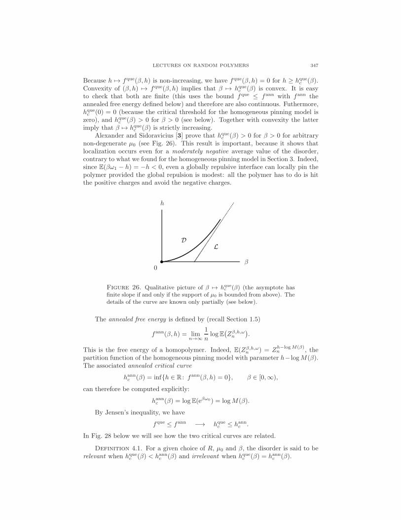
The excursions of S away from the interface cut out successive words from therandom environment ω, forming an infinite sentence (see Fig. 27). Under the joint
law of S and ω, this sentence has law q⊗N
0 with
q0(dx0, . . . , dxk−1) = R(k)µ0(dx0)×· · ·×µ0(dxk−1), k ∈ N, x0, . . . , xk−1 ∈ R.
Figure 27. Infinite sentence generated by S on ω.
For Q ∈ P inv(RN), let
Ique(Q) = H(Q | q⊗N
0
)+ amQH
(ΨQ |µ⊗N0
0
),
Iann(Q) = H(Q | q⊗N
0
),
LECTURES ON RANDOM POLYMERS 349
where
• ΨQ ∈ P(RN0) is the projection of Q via concatenation of words;• mQ is the average word length under Q;• H(·|·) denotes specific relative entropy.
It is shown in Birkner, Greven and den Hollander [12] that Ique and Iann are thequenched and the annealed rate function in the large deviation principle (LDP) forthe empirical process of words. More precisely,
exp[−NIque(Q) + o(N)] and exp[−NIann(Q) + o(N)]
are the respective probabilities that the first N words generated by S on ω, period-ically extended to form an infinite sentence, have an empirical distribution that is
close to Q ∈ P inv(RN) in the weak topology. Tutorial 4 in Appendix D providesthe background of this LDP.
The main message of the formulas for Ique(Q) and Iann(Q) is that
Ique(Q) = Iann(Q) + an explicit extra term.
We will see in Section 4.4 that the extra term is crucial for the distinction betweenrelevant and irrelevant disorder.
4.4. Application of the LDP. For Q ∈ P inv(RN), let π1,1Q ∈ P(R) denotethe projection of Q onto the first letter of the first word. Define Φ(Q) to be theaverage value of the first letter under Q,
Φ(Q) =
∫
R
x (π1,1Q)(dx), Q ∈ P inv(RN),
and C to be the set
C =Q ∈ P inv(RN) :
∫
R
|x| (π1,1Q)(dx) <∞.
The following theorem provides variational formulas for the critical curves.
Theorem 4.2. [Cheliotis and den Hollander [35]] Fix µ0 and R. For all β ∈[0,∞),
hquec (β) = supQ∈C
[βΦ(Q)− Ique(Q)],
hannc (β) = supQ∈C
[βΦ(Q)− Iann(Q)].
For β ∈ [0,∞), let
µβ(dx) =1
M(β)eβx µ0(dx), x ∈ R,
and let Qβ = q⊗N
β ∈ P inv(RN) be the law of the infinite sentence generated by S onω when the first letter of each word is drawn from the tilted law µβ rather than µ0,i.e.,
qβ(dx0, . . . , dxn−1) = R(n)µβ(dx0)×· · ·×µ0(dxn−1), n ∈ N, x0, . . . , xn−1 ∈ R.
It turns out that Qβ is the unique maximizer of the annealed variational formula.This leads to the following two theorems.
350 CARAVENNA, DEN HOLLANDER, AND PETRELIS
Theorem 4.3. [Cheliotis and den Hollander [35]] Fix µ0 and R. For all β ∈[0,∞),
hquec (β) < hannc (β) ⇐⇒ Ique(Qβ) > Iann(Qβ).
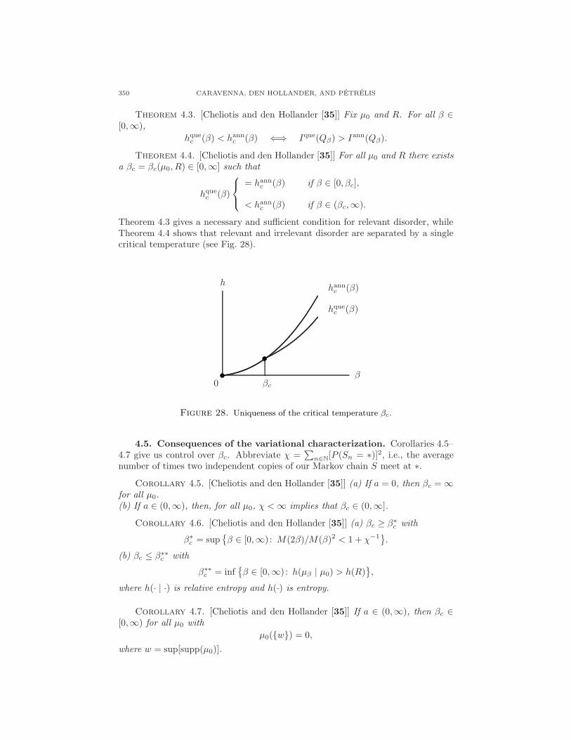
Theorem 4.4. [Cheliotis and den Hollander [35]] For all µ0 and R there existsa βc = βc(µ0, R) ∈ [0,∞] such that
hquec (β)
= hannc (β) if β ∈ [0, βc],
< hannc (β) if β ∈ (βc,∞).
Theorem 4.3 gives a necessary and sufficient condition for relevant disorder, whileTheorem 4.4 shows that relevant and irrelevant disorder are separated by a singlecritical temperature (see Fig. 28).
0β
h
hquec (β)
hannc (β)
βc
Figure 28. Uniqueness of the critical temperature βc.
4.5. Consequences of the variational characterization. Corollaries 4.5–4.7 give us control over βc. Abbreviate χ =
∑n∈N
[P (Sn = ∗)]2, i.e., the averagenumber of times two independent copies of our Markov chain S meet at ∗.
Corollary 4.5. [Cheliotis and den Hollander [35]] (a) If a = 0, then βc = ∞for all µ0.(b) If a ∈ (0,∞), then, for all µ0, χ <∞ implies that βc ∈ (0,∞].
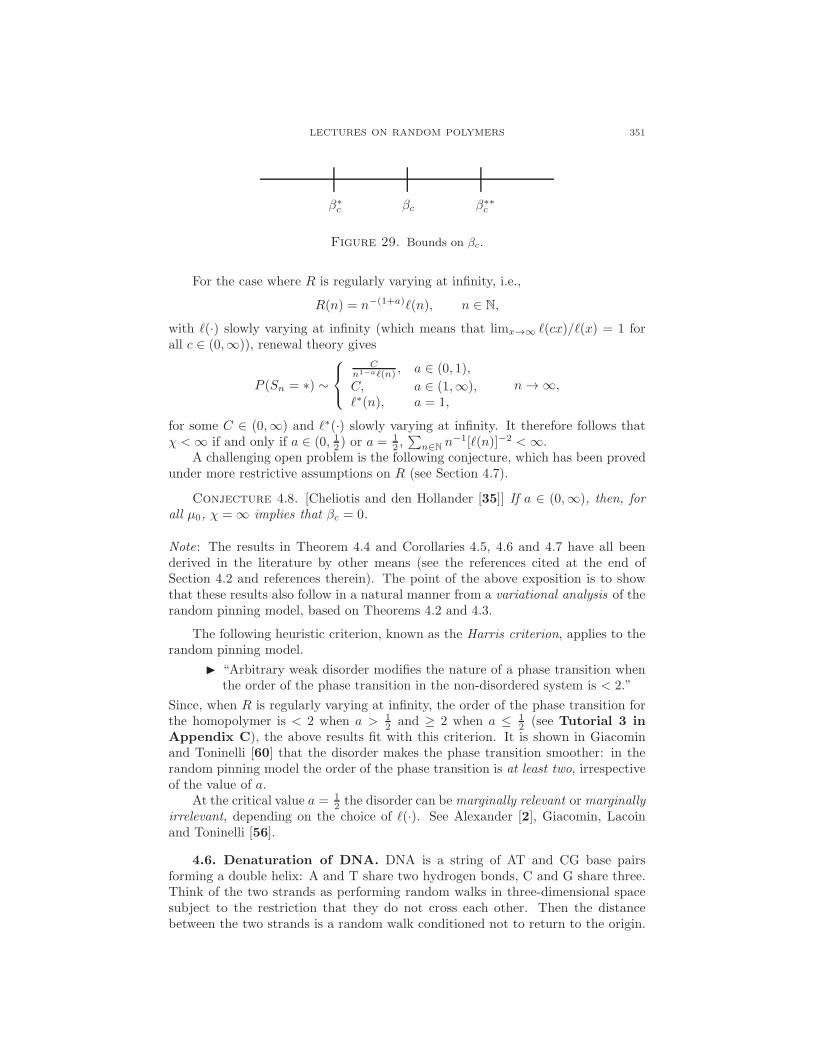
Corollary 4.6. [Cheliotis and den Hollander [35]] (a) βc ≥ β∗c with
β∗c = sup
β ∈ [0,∞) : M(2β)/M(β)2 < 1 + χ−1
.
(b) βc ≤ β∗∗c with
β∗∗c = inf
β ∈ [0,∞) : h(µβ | µ0) > h(R)
,
where h(· | ·) is relative entropy and h(·) is entropy.
Corollary 4.7. [Cheliotis and den Hollander [35]] If a ∈ (0,∞), then βc ∈[0,∞) for all µ0 with
µ0(w) = 0,
where w = sup[supp(µ0)].
LECTURES ON RANDOM POLYMERS 351
βcβ∗c β∗∗
c
Figure 29. Bounds on βc.
For the case where R is regularly varying at infinity, i.e.,
R(n) = n−(1+a)ℓ(n), n ∈ N,
with ℓ(·) slowly varying at infinity (which means that limx→∞ ℓ(cx)/ℓ(x) = 1 forall c ∈ (0,∞)), renewal theory gives
P (Sn = ∗) ∼
Cn1−aℓ(n) , a ∈ (0, 1),
C, a ∈ (1,∞),ℓ∗(n), a = 1,
n→ ∞,
for some C ∈ (0,∞) and ℓ∗(·) slowly varying at infinity. It therefore follows thatχ <∞ if and only if a ∈ (0, 12 ) or a = 1
2 ,∑n∈N
n−1[ℓ(n)]−2 <∞.A challenging open problem is the following conjecture, which has been proved
under more restrictive assumptions on R (see Section 4.7).
Conjecture 4.8. [Cheliotis and den Hollander [35]] If a ∈ (0,∞), then, forall µ0, χ = ∞ implies that βc = 0.
Note: The results in Theorem 4.4 and Corollaries 4.5, 4.6 and 4.7 have all beenderived in the literature by other means (see the references cited at the end ofSection 4.2 and references therein). The point of the above exposition is to showthat these results also follow in a natural manner from a variational analysis of therandom pinning model, based on Theorems 4.2 and 4.3.
The following heuristic criterion, known as the Harris criterion, applies to therandom pinning model.
“Arbitrary weak disorder modifies the nature of a phase transition whenthe order of the phase transition in the non-disordered system is < 2.”
Since, when R is regularly varying at infinity, the order of the phase transition forthe homopolymer is < 2 when a > 1
2 and ≥ 2 when a ≤ 12 (see Tutorial 3 in
Appendix C), the above results fit with this criterion. It is shown in Giacominand Toninelli [60] that the disorder makes the phase transition smoother: in therandom pinning model the order of the phase transition is at least two, irrespectiveof the value of a.
At the critical value a = 12 the disorder can bemarginally relevant or marginally
irrelevant, depending on the choice of ℓ(·). See Alexander [2], Giacomin, Lacoinand Toninelli [56].
4.6. Denaturation of DNA. DNA is a string of AT and CG base pairsforming a double helix: A and T share two hydrogen bonds, C and G share three.Think of the two strands as performing random walks in three-dimensional spacesubject to the restriction that they do not cross each other. Then the distancebetween the two strands is a random walk conditioned not to return to the origin.
352 CARAVENNA, DEN HOLLANDER, AND PETRELIS
Since three-dimensional random walks are transient, this condition has an effectsimilar to that of a hard wall.
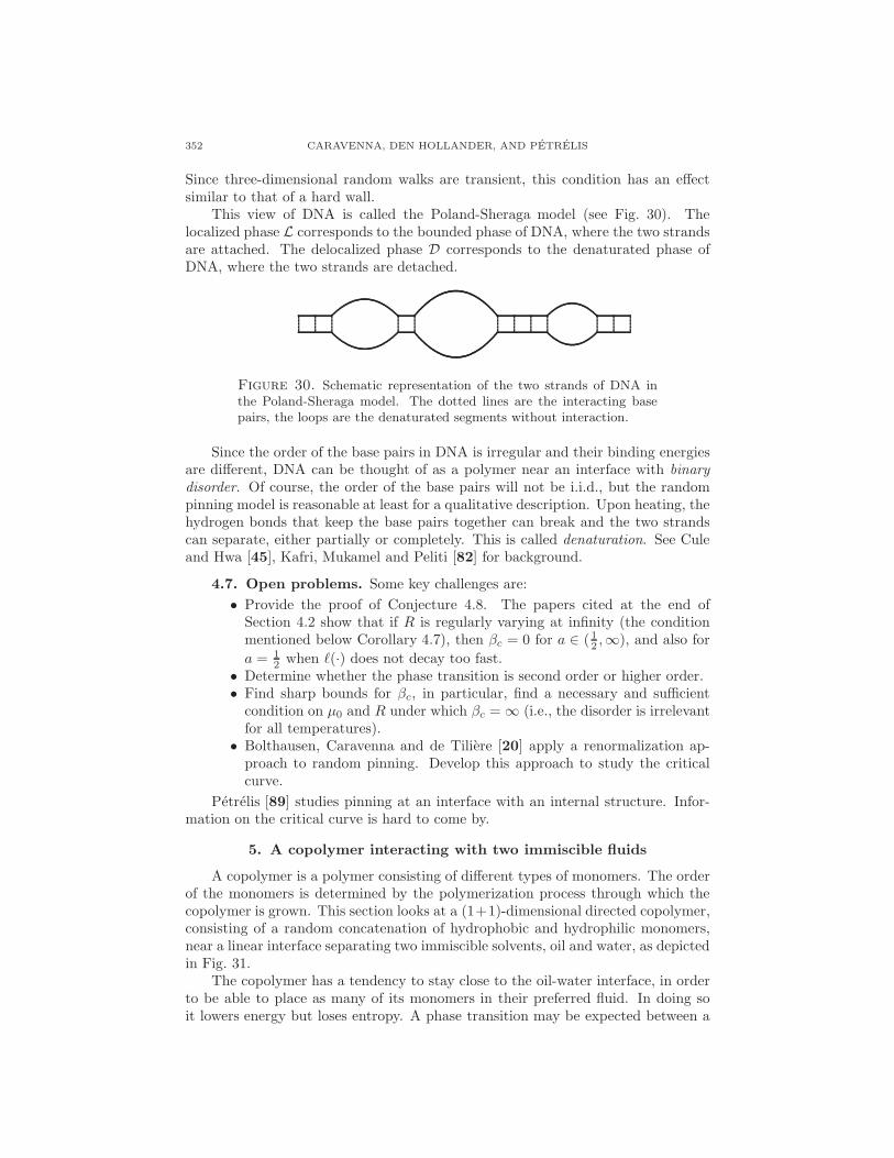
This view of DNA is called the Poland-Sheraga model (see Fig. 30). Thelocalized phase L corresponds to the bounded phase of DNA, where the two strandsare attached. The delocalized phase D corresponds to the denaturated phase ofDNA, where the two strands are detached.
Figure 30. Schematic representation of the two strands of DNA inthe Poland-Sheraga model. The dotted lines are the interacting basepairs, the loops are the denaturated segments without interaction.
Since the order of the base pairs in DNA is irregular and their binding energiesare different, DNA can be thought of as a polymer near an interface with binarydisorder. Of course, the order of the base pairs will not be i.i.d., but the randompinning model is reasonable at least for a qualitative description. Upon heating, thehydrogen bonds that keep the base pairs together can break and the two strandscan separate, either partially or completely. This is called denaturation. See Culeand Hwa [45], Kafri, Mukamel and Peliti [82] for background.
4.7. Open problems. Some key challenges are:
• Provide the proof of Conjecture 4.8. The papers cited at the end ofSection 4.2 show that if R is regularly varying at infinity (the conditionmentioned below Corollary 4.7), then βc = 0 for a ∈ (12 ,∞), and also for
a = 12 when ℓ(·) does not decay too fast.
• Determine whether the phase transition is second order or higher order.• Find sharp bounds for βc, in particular, find a necessary and sufficientcondition on µ0 and R under which βc = ∞ (i.e., the disorder is irrelevantfor all temperatures).
• Bolthausen, Caravenna and de Tiliere [20] apply a renormalization ap-proach to random pinning. Develop this approach to study the criticalcurve.
Petrelis [89] studies pinning at an interface with an internal structure. Infor-mation on the critical curve is hard to come by.
5. A copolymer interacting with two immiscible fluids
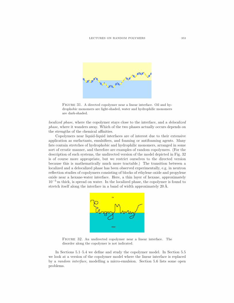
A copolymer is a polymer consisting of different types of monomers. The orderof the monomers is determined by the polymerization process through which thecopolymer is grown. This section looks at a (1+1)-dimensional directed copolymer,consisting of a random concatenation of hydrophobic and hydrophilic monomers,near a linear interface separating two immiscible solvents, oil and water, as depictedin Fig. 31.
The copolymer has a tendency to stay close to the oil-water interface, in orderto be able to place as many of its monomers in their preferred fluid. In doing soit lowers energy but loses entropy. A phase transition may be expected between a
LECTURES ON RANDOM POLYMERS 353
Figure 31. A directed copolymer near a linear interface. Oil and hy-drophobic monomers are light-shaded, water and hydrophilic monomersare dark-shaded.
localized phase, where the copolymer stays close to the interface, and a delocalizedphase, where it wanders away. Which of the two phases actually occurs depends onthe strengths of the chemical affinities.
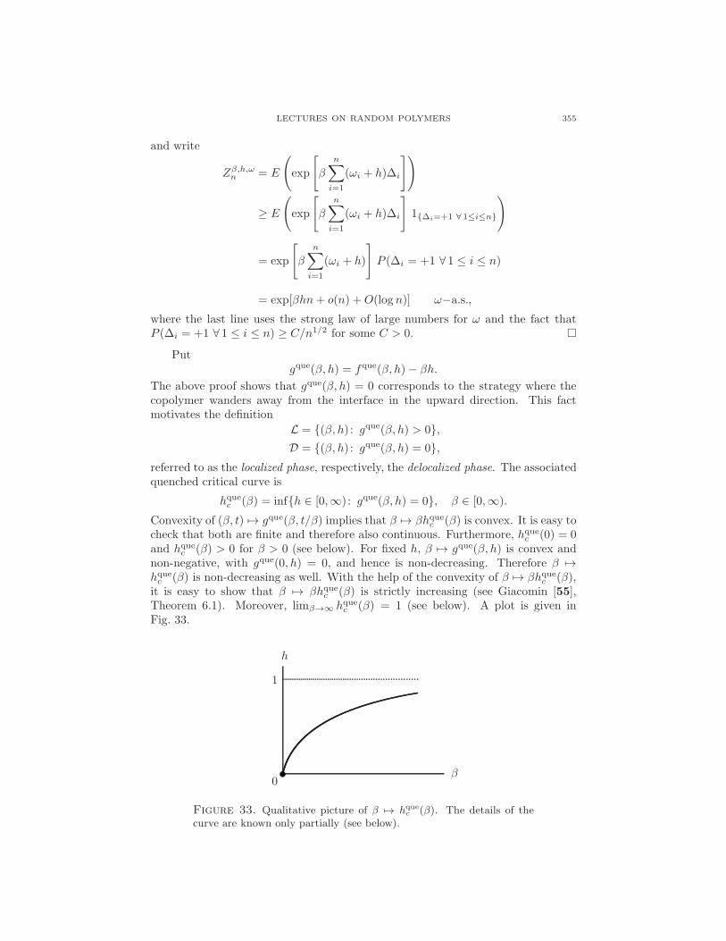
Copolymers near liquid-liquid interfaces are of interest due to their extensiveapplication as surfactants, emulsifiers, and foaming or antifoaming agents. Manyfats contain stretches of hydrophobic and hydrophilic monomers, arranged in somesort of erratic manner, and therefore are examples of random copolymers. (For thedescription of such systems, the undirected version of the model depicted in Fig. 32is of course more appropriate, but we restrict ourselves to the directed versionbecause this is mathematically much more tractable.) The transition between alocalized and a delocalized phase has been observed experimentally, e.g. in neutronreflection studies of copolymers consisting of blocks of ethylene oxide and propyleneoxide near a hexane-water interface. Here, a thin layer of hexane, approximately10−5m thick, is spread on water. In the localized phase, the copolymer is found tostretch itself along the interface in a band of width approximately 20 A.
Water
Oil
Figure 32. An undirected copolymer near a linear interface. Thedisorder along the copolymer is not indicated.
In Sections 5.1–5.4 we define and study the copolymer model. In Section 5.5we look at a version of the copolymer model where the linear interface is replacedby a random interface, modelling a micro-emulsion. Section 5.6 lists some openproblems.

354 CARAVENNA, DEN HOLLANDER, AND PETRELIS
5.1. Model. Let
Wn =w = (i, wi)
ni=0 : w0 = 0, wi+1 − wi = ±1 ∀ 0 ≤ i < n
denote the set of all n-step directed paths that start from the origin and at eachstep move either north-east or south-east. Let
ω = (ωi)i∈N be i.i.d. with P(ω1 = +1) = P(ω1 = −1) = 12
label the order of the monomers along the copolymer. Write P to denote the lawof ω. The Hamiltonian, for fixed ω, is
Hβ,h,ωn (w) = −β
n∑
i=1
(ωi + h) sign(wi−1, wi), w ∈ Wn,
with β, h ∈ [0,∞) the disorder strength, respectively, the disorder bias (the meaningof sign(wi−1, wi) is explained below). The path measure, for fixed ω, is
P β,h,ωn (w) =1
Zβ,h,ωn
e−Hβ,h,ωn (w) Pn(w), w ∈ Wn,
where Pn is the law of the n-step directed random walk, which is the uniformdistribution on Wn. Note that Pn is the projection on Wn of the law P of theinfinite directed walk whose vertical steps are SRW.
The interpretation of the above definitions is as follows: ωi = +1 or −1 standsfor monomer i being hydrophobic or hydrophilic; sign(wi−1, wi) = +1 or −1 standsfor monomer i lying in oil or water; −β(ωi + h)sign(wi−1, wi) is the energy ofmonomer i. For h = 0 both monomer types interact equally strongly, while forh = 1 the hydrophilic monomers do not interact at all. Thus, only the regimeh ∈ [0, 1] is relevant, and for h > 0 the copolymer prefers the oil over the water.
Note that the energy of a path is a sum of contributions coming from itssuccessive excursions away from the interface (this viewpoint was already exploitedin Section 4 for the random pinning model). All that is relevant for the energy of theexcursions is what stretch of ω they sample, and whether they are above or belowthe interface. The copolymer model is harder than the random pinning model,because the energy of an excursion depends on the sum of the values of ω in thestretch that is sampled, not just on the first value. We expect the localized phaseto occur for large β and/or small h and the delocalized phase for small β and/orlarge h. Our goal is to identify the critical curve separating the two phases.
5.2. Free energies. The quenched free energy is defined as
fque(β, h) = limn→∞
1
nlogZβ,h,ωn ω−a.s.
Subadditivity arguments show that ω-a.s. the limit exists and is non-random for allβ, h ∈ [0,∞) (see Tutorial 1 in Appendix A). The following lower bound holds:
fque(β, h) ≥ βh ∀β, h ∈ [0,∞).
Proof. Abbreviate
∆i = sign(Si−1, Si)
LECTURES ON RANDOM POLYMERS 355
and write
Zβ,h,ωn = E
(exp
[β
n∑
i=1
(ωi + h)∆i
])
≥ E
(exp
[β
n∑
i=1
(ωi + h)∆i
]1∆i=+1 ∀ 1≤i≤n
)
= exp
[β
n∑
i=1
(ωi + h)
]P (∆i = +1 ∀ 1 ≤ i ≤ n)
= exp[βhn+ o(n) +O(log n)] ω−a.s.,
where the last line uses the strong law of large numbers for ω and the fact thatP (∆i = +1 ∀ 1 ≤ i ≤ n) ≥ C/n1/2 for some C > 0.
Putgque(β, h) = fque(β, h)− βh.
The above proof shows that gque(β, h) = 0 corresponds to the strategy where thecopolymer wanders away from the interface in the upward direction. This factmotivates the definition
L = (β, h) : gque(β, h) > 0,D = (β, h) : gque(β, h) = 0,
referred to as the localized phase, respectively, the delocalized phase. The associatedquenched critical curve is
hquec (β) = infh ∈ [0,∞) : gque(β, h) = 0, β ∈ [0,∞).
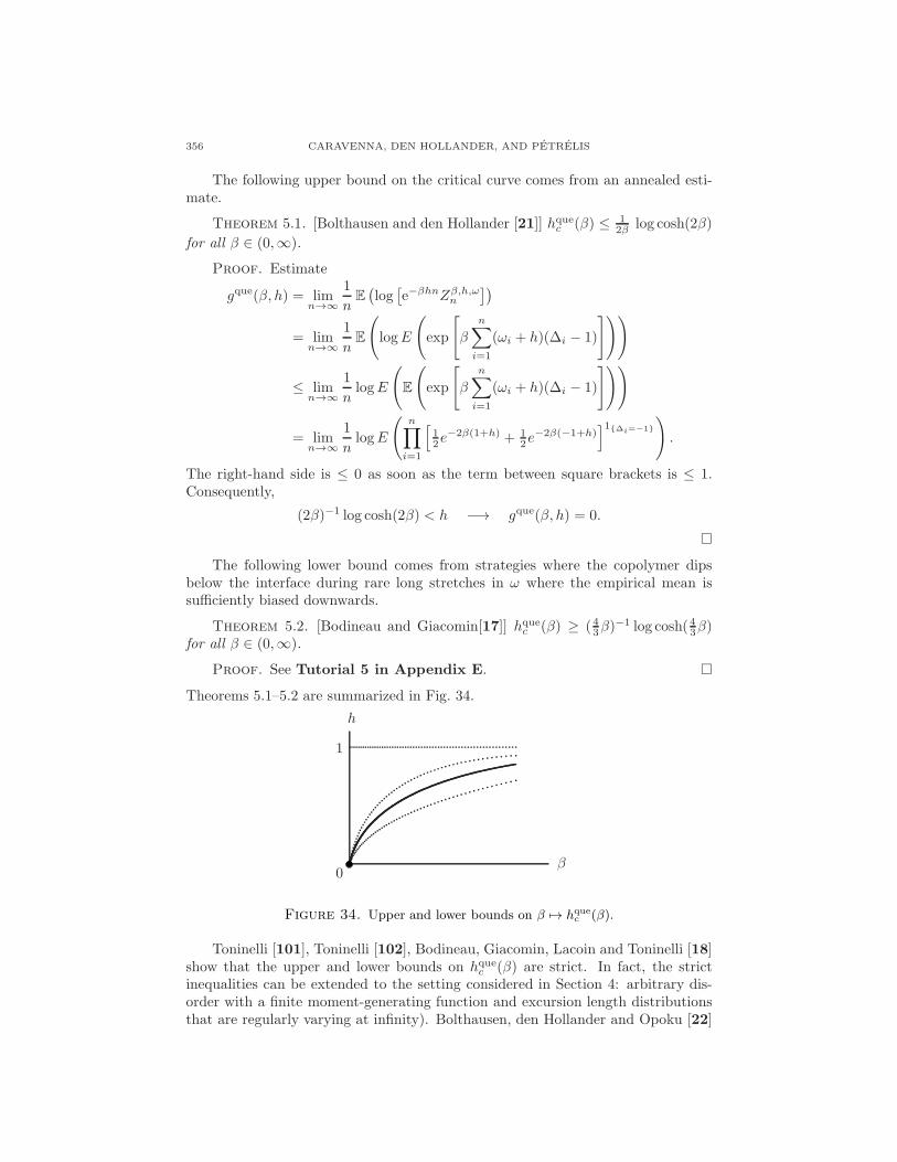
Convexity of (β, t) 7→ gque(β, t/β) implies that β 7→ βhquec (β) is convex. It is easy tocheck that both are finite and therefore also continuous. Furthermore, hquec (0) = 0and hquec (β) > 0 for β > 0 (see below). For fixed h, β 7→ gque(β, h) is convex andnon-negative, with gque(0, h) = 0, and hence is non-decreasing. Therefore β 7→hquec (β) is non-decreasing as well. With the help of the convexity of β 7→ βhquec (β),it is easy to show that β 7→ βhquec (β) is strictly increasing (see Giacomin [55],Theorem 6.1). Moreover, limβ→∞ hquec (β) = 1 (see below). A plot is given inFig. 33.
0β
h
1
Figure 33. Qualitative picture of β 7→ hquec (β). The details of the
curve are known only partially (see below).
356 CARAVENNA, DEN HOLLANDER, AND PETRELIS
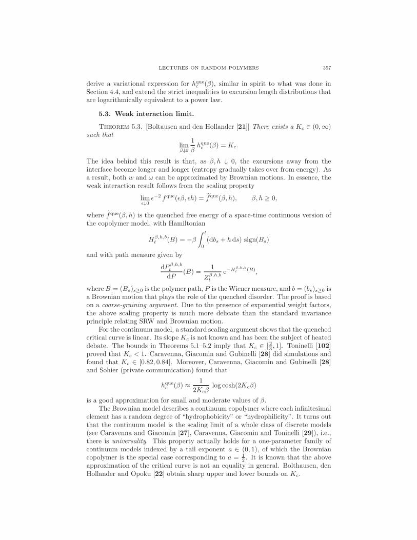
The following upper bound on the critical curve comes from an annealed esti-mate.
Theorem 5.1. [Bolthausen and den Hollander [21]] hquec (β) ≤ 12β log cosh(2β)
for all β ∈ (0,∞).
Proof. Estimate
gque(β, h) = limn→∞
1
nE(log[e−βhnZβ,h,ωn
])
= limn→∞
1
nE
(logE
(exp
[β
n∑
i=1
(ωi + h)(∆i − 1)
]))
≤ limn→∞
1
nlogE
(E
(exp
[β
n∑
i=1
(ωi + h)(∆i − 1)
]))
= limn→∞
1
nlogE
(n∏
i=1
[12e
−2β(1+h) + 12e
−2β(−1+h)]1∆i=−1
).
The right-hand side is ≤ 0 as soon as the term between square brackets is ≤ 1.Consequently,
(2β)−1 log cosh(2β) < h −→ gque(β, h) = 0.
The following lower bound comes from strategies where the copolymer dipsbelow the interface during rare long stretches in ω where the empirical mean issufficiently biased downwards.
Theorem 5.2. [Bodineau and Giacomin[17]] hquec (β) ≥ (43β)−1 log cosh(43β)
for all β ∈ (0,∞).
Proof. See Tutorial 5 in Appendix E.
Theorems 5.1–5.2 are summarized in Fig. 34.
0β
h
1
Figure 34. Upper and lower bounds on β 7→ hquec (β).
Toninelli [101], Toninelli [102], Bodineau, Giacomin, Lacoin and Toninelli [18]show that the upper and lower bounds on hquec (β) are strict. In fact, the strictinequalities can be extended to the setting considered in Section 4: arbitrary dis-order with a finite moment-generating function and excursion length distributionsthat are regularly varying at infinity). Bolthausen, den Hollander and Opoku [22]
LECTURES ON RANDOM POLYMERS 357
derive a variational expression for hquec (β), similar in spirit to what was done inSection 4.4, and extend the strict inequalities to excursion length distributions thatare logarithmically equivalent to a power law.
5.3. Weak interaction limit.
Theorem 5.3. [Boltausen and den Hollander [21]] There exists a Kc ∈ (0,∞)such that
limβ↓0
1
βhquec (β) = Kc.
The idea behind this result is that, as β, h ↓ 0, the excursions away from theinterface become longer and longer (entropy gradually takes over from energy). Asa result, both w and ω can be approximated by Brownian motions. In essence, theweak interaction result follows from the scaling property
limǫ↓0
ǫ−2 fque(ǫβ, ǫh) = fque(β, h), β, h ≥ 0,
where fque(β, h) is the quenched free energy of a space-time continuous version ofthe copolymer model, with Hamiltonian
Hβ,h,bt (B) = −β
∫ t
0
(dbs + h ds) sign(Bs)
and with path measure given by
dP β,h,bt
dP(B) =
1
Zβ,h,bt
e−Hβ,h,bt (B),
whereB = (Bs)s≥0 is the polymer path, P is the Wiener measure, and b = (bs)s≥0 isa Brownian motion that plays the role of the quenched disorder. The proof is basedon a coarse-graining argument. Due to the presence of exponential weight factors,the above scaling property is much more delicate than the standard invarianceprinciple relating SRW and Brownian motion.
For the continuummodel, a standard scaling argument shows that the quenchedcritical curve is linear. Its slope Kc is not known and has been the subject of heateddebate. The bounds in Theorems 5.1–5.2 imply that Kc ∈ [ 23 , 1]. Toninelli [102]proved that Kc < 1. Caravenna, Giacomin and Gubinelli [28] did simulations andfound that Kc ∈ [0.82, 0.84]. Moreover, Caravenna, Giacomin and Gubinelli [28]and Sohier (private communication) found that
hquec (β) ≈ 1
2Kcβlog cosh(2Kcβ)
is a good approximation for small and moderate values of β.The Brownian model describes a continuum copolymer where each infinitesimal
element has a random degree of “hydrophobicity” or “hydrophilicity”. It turns outthat the continuum model is the scaling limit of a whole class of discrete models(see Caravenna and Giacomin [27], Caravenna, Giacomin and Toninelli [29]), i.e.,there is universality. This property actually holds for a one-parameter family ofcontinuum models indexed by a tail exponent a ∈ (0, 1), of which the Browniancopolymer is the special case corresponding to a = 1
2 . It is known that the aboveapproximation of the critical curve is not an equality in general. Bolthausen, denHollander and Opoku [22] obtain sharp upper and lower bounds on Kc.
358 CARAVENNA, DEN HOLLANDER, AND PETRELIS
A related coarse-graining result is proved in Petrelis [91] for a copolymer modelwith additional random pinning in a finite layer around the interface (of the typeconsidered in Section 4). It is shown that the effect of the disorder in the layervanishes in the weak interaction limit, i.e., only the disorder along the copolymeris felt in the weak interaction limit.
5.4. Qualitative properties of the phases. We proceed by stating a fewpath properties in the two phases.
Theorem 5.4. [Biskup and den Hollander [16], Giacomin and Toninelli [58,61]] (a) If (β, h) ∈ L, then the path intersects the interface with a strictly positivedensity, while the length and the height of the largest excursion away from theinterface up to time n is order logn.(b) If (β, h) ∈ int(D), then the path intersects the interface with zero density. Thenumber of intersections is O(log n).
For (β, h) ∈ int(D), the number of intersections is expected to be O(1) under theaverage quenched path measure (see Part III of Section 1.5). So far this has onlybeen proved for (β, h) above the annealed upper bound.
Theorem 5.5. [Giacomin and Toninelli [59, 60]] For every β ∈ (0,∞),
0 ≤ gque(β, h) = O([hquec (β) − h]2
)as h ↑ hquec (β).
Theorem 5.6. [Giacomin and Toninelli [61]] (β, h) 7→ fque(β, h) is infinitelydifferentiable on L.Theorem 5.5 says that the phase transition is at least second order, while Theo-rem 5.6 says that the critical curve is the only location where a phase transition offinite order occurs. Theorem 5.5 is proved in Tutorial 5 in Appendix E.
All of the results in Sections 5.2–5.4 extend to ωi ∈ R rather than ωi ∈−1,+1, provided the law of ωi has a finite moment-generating function, and tomore general excursion length distributions, of the type considered in Section 4.1.For an overview, see Caravenna, Giacomin and Toninelli [29].
5.5. A copolymer in a micro-emulsion. What happens when the linearinterface is replaced by a random interface? In particular, what happens when theoil forms droplets that float around in the water, as in Fig. 35? An example is milk,which is a micro-emulsion consisting (among others) of water and tiny fat-droplets.Milk is stabilized by a protein called casein, a copolymer that wraps itself aroundthe droplets and prevents them to coagulate.
A phase transition may be expected between a localized phase, where the copoly-mer spends most of its time near the boundary of the droplets and makes rapidhops from one droplet to the other, and a delocalized phase, where it spends mostof its time inside and outside of droplets. We will see that the actual behavior israther more complicated. This is due to the fact that there are three (!) types ofrandomness in the model: a random polymer path, a random ordering of monomertypes, and a random arrangement of droplets in the emulsion.
Here is a quick definition of a model. Split Z2 into square blocks of size Ln. Thecopolymer follows a directed self-avoiding path that is allowed to make steps ↑, ↓,→and to enter and exit blocks at diagonally opposite corners (see Fig. 36). Eachmonomer has probability 1
2 to be hydrophobic and probability 12 to be hydrophilic,
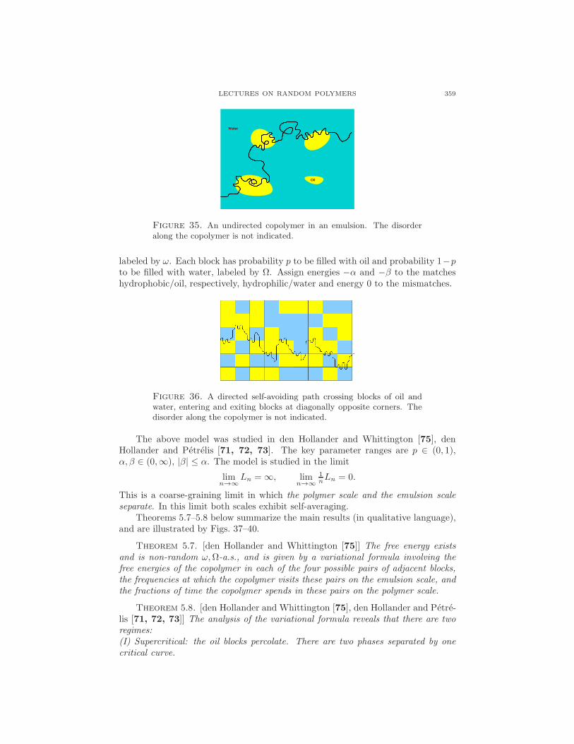
LECTURES ON RANDOM POLYMERS 359
Water
Oil
Figure 35. An undirected copolymer in an emulsion. The disorderalong the copolymer is not indicated.
labeled by ω. Each block has probability p to be filled with oil and probability 1−pto be filled with water, labeled by Ω. Assign energies −α and −β to the matcheshydrophobic/oil, respectively, hydrophilic/water and energy 0 to the mismatches.
Figure 36. A directed self-avoiding path crossing blocks of oil andwater, entering and exiting blocks at diagonally opposite corners. Thedisorder along the copolymer is not indicated.
The above model was studied in den Hollander and Whittington [75], denHollander and Petrelis [71, 72, 73]. The key parameter ranges are p ∈ (0, 1),α, β ∈ (0,∞), |β| ≤ α. The model is studied in the limit
limn→∞
Ln = ∞, limn→∞
1nLn = 0.
This is a coarse-graining limit in which the polymer scale and the emulsion scaleseparate. In this limit both scales exhibit self-averaging.
Theorems 5.7–5.8 below summarize the main results (in qualitative language),and are illustrated by Figs. 37–40.
Theorem 5.7. [den Hollander and Whittington [75]] The free energy existsand is non-random ω,Ω-a.s., and is given by a variational formula involving thefree energies of the copolymer in each of the four possible pairs of adjacent blocks,the frequencies at which the copolymer visits these pairs on the emulsion scale, andthe fractions of time the copolymer spends in these pairs on the polymer scale.
Theorem 5.8. [den Hollander and Whittington [75], den Hollander and Petre-lis [71, 72, 73]] The analysis of the variational formula reveals that there are tworegimes:(I) Supercritical: the oil blocks percolate. There are two phases separated by onecritical curve.
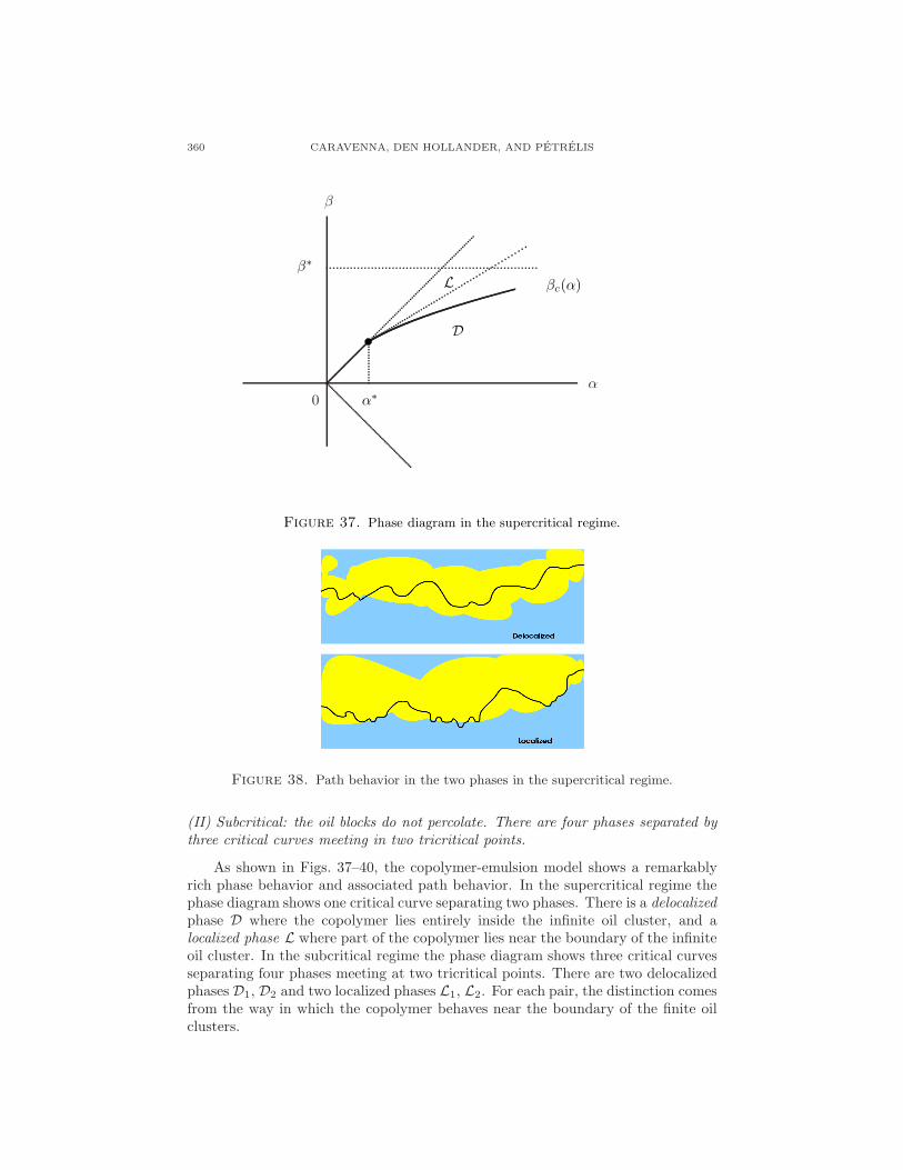
360 CARAVENNA, DEN HOLLANDER, AND PETRELIS
0α
β
α∗
β∗
βc(α)L
D
Figure 37. Phase diagram in the supercritical regime.
Figure 38. Path behavior in the two phases in the supercritical regime.
(II) Subcritical: the oil blocks do not percolate. There are four phases separated bythree critical curves meeting in two tricritical points.
As shown in Figs. 37–40, the copolymer-emulsion model shows a remarkablyrich phase behavior and associated path behavior. In the supercritical regime thephase diagram shows one critical curve separating two phases. There is a delocalizedphase D where the copolymer lies entirely inside the infinite oil cluster, and alocalized phase L where part of the copolymer lies near the boundary of the infiniteoil cluster. In the subcritical regime the phase diagram shows three critical curvesseparating four phases meeting at two tricritical points. There are two delocalizedphases D1, D2 and two localized phases L1, L2. For each pair, the distinction comesfrom the way in which the copolymer behaves near the boundary of the finite oilclusters.
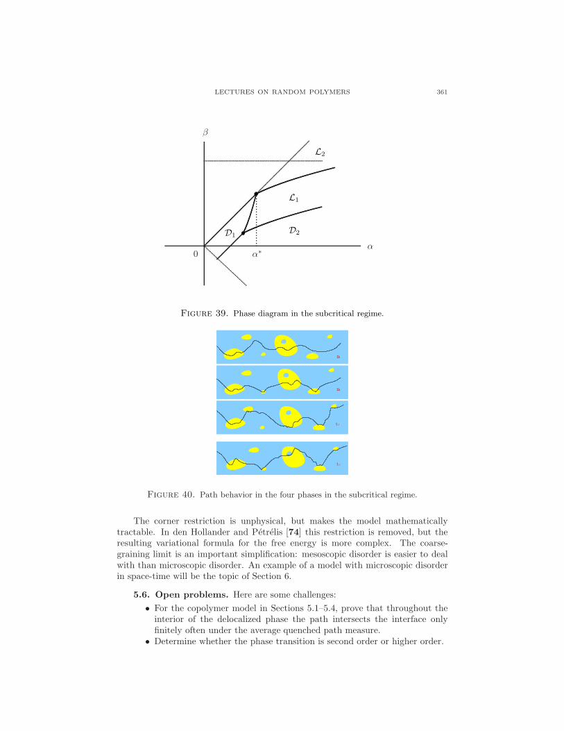
LECTURES ON RANDOM POLYMERS 361
0α
β
α∗
D1D2
L1
L2
Figure 39. Phase diagram in the subcritical regime.
L
1
2
1D
D
L
2
Figure 40. Path behavior in the four phases in the subcritical regime.
The corner restriction is unphysical, but makes the model mathematicallytractable. In den Hollander and Petrelis [74] this restriction is removed, but theresulting variational formula for the free energy is more complex. The coarse-graining limit is an important simplification: mesoscopic disorder is easier to dealwith than microscopic disorder. An example of a model with microscopic disorderin space-time will be the topic of Section 6.
5.6. Open problems. Here are some challenges:
• For the copolymer model in Sections 5.1–5.4, prove that throughout theinterior of the delocalized phase the path intersects the interface onlyfinitely often under the average quenched path measure.
• Determine whether the phase transition is second order or higher order.

362 CARAVENNA, DEN HOLLANDER, AND PETRELIS
• Compute the critical slope Kc of the Brownian copolymer.• For the copolymer/emulsion model in Section 5.5, determine the fine de-tails of the phase diagrams in Figs. 37 and 39, and of the path propertiesin Figs. 38 and 40.
6. A polymer in a random potential
This section takes a look at a (1+d)-dimensional directed polymer in a randompotential: the polymer and the potential live on N× Z
d, where N is time and Zd,
d ≥ 1, is space (see Fig. 41). In Section 6.1 we define the model. In Sections 6.2–6.4we study the two phases that occur: the weak disorder phase, in which the polymerlargely ignores the disorder and behaves diffusively, and the strong disorder phase,in which the polymer hunts for favorable spots in the disorder and behaves superdif-fusively. In Section 6.5 we derive bounds on the critical temperature separating thetwo phases. Section 6.6 lists a few open problems.
Figure 41. A directed polymer in a random potential. Differentshades of white, grey and black represent different values of the poten-
tial.
6.1. Model. The set of paths is
Wn =w = (i, wi)
ni=0 :
w0 = 0, ‖wi+1 − wi‖ = 1 ∀ 0 ≤ i < n.
The random environment
ω = ω(i, x) : i ∈ N, x ∈ Zd
consists of an i.i.d. field of R-valued non-degenerate random variables with momentgenerating function
M(β) = E(eβω(1,0)
)<∞ ∀β ∈ [0,∞),
where P denotes the law of ω. The Hamiltonian is
Hβ,ωn (w) = −β
n∑
i=1
ω(i, wi), w ∈ Wn,
LECTURES ON RANDOM POLYMERS 363
where β plays the role of the disorder strength. The associated quenched pathmeasure is
P β,ωn (w) =1
Zβ,ωn
e−Hβ,ωn (w) Pn(w), w ∈ Wn,
where Pn is the projection onto Wn of the law P of directed SRW on Zd.
We may think of the model as a version of the “copolymer in emulsion” de-scribed in Section 5.5 where the disorder is microscopic rather than mesoscopic.There are deep relations with several other models in probability theory and statis-tical physics, including growth and wave-front-propagationmodels and first-passagepercolation. Indeed, for β = ∞ the polymer follows the path along which the sumof the disorder is largest. This case corresponds to oriented first-passage percola-tion, of which some aspects are discussed in the lectures by Garban and Steif [54].For β <∞ the model is sometimes referred to as oriented first-passage percolationat positive temperature.
The key object in the analysis of the model is the following quantity:
Y β,ωn =Zβ,ωn
E(Zβ,ωn ), n ∈ N0.
This is the ratio of the quenched and the annealed partition sum. The point is that
(Y β,ωn )n∈N0
is a martingale w.r.t. the natural filtration generated by ω, i.e., F = (Fn)n∈N0with
Fn = σ(ω(i, x) : 0 ≤ i ≤ n, x ∈ Zd). Indeed, this is seen by writing
Y β,ωn = E
(n∏
i=1
[eβω(i,Si)
M(β)
]), Y β,ω0 = 1,
from which it is easily deduced that E(Y β,ωn |Fn−1) = Y β,ωn−1. Note that E(Yβ,ωn ) = 1
and Y β,ωn > 0 for all n ∈ N0.
6.2. A dichotomy: weak and strong disorder. Since Y β,ωn ≥ 0, it followsfrom the martingale convergence theorem that
Y β,ω = limn→∞
Y β,ωn exists ω-a.s.
Moreover, since the event ω : Y β,ω > 0 is measurable w.r.t. the tail sigma-algebraof ω, it follows from the Kolmogorov zero-one law that the following dichotomyholds:
(WD): P(Y β,ω > 0) = 1,(SD): P(Y β,ω = 0) = 1.
In what follows it will turn out that (WD) characterizes weak disorder, for whichthe behavior of the polymer is diffusive in the Z
d-direction, while (SD) character-izes strong disorder, for which the behavior is (expected to be) superdiffusive (seeFig. 42). Note that the nomenclature is appropriate: in phase (WD) the quenchedand the annealed partition sum remain comparable in the limit as n → ∞, in-dicating a weak role for the disorder, while in phase (SD) the annealed partitionsum grows faster than the quenched partition sum, indicating a strong role for thedisorder.

364 CARAVENNA, DEN HOLLANDER, AND PETRELIS
Figure 42. Typical path behavior in the two phases.
6.3. Separation of the two phases.
Theorem 6.1. [Comets and Yoshida [42]] For any choice of the disorder dis-
tribution, β 7→ E(√Y β,ω) is non-increasing on [0,∞). Consequently, there exists a
βc ∈ [0,∞] such that (see Fig. 43)
β ∈ [0, βc) −→ (WD),
β ∈ (βc,∞) −→ (SD).
βc
?(WD) (SD)
Figure 43. Separation of the two phases. It is not known which ofthe two phases includes βc.
Since
fque(β) = limn→∞
1
nlogZβ,ωn ω-a.s.,
fann(β) = limn→∞
1
nlogE(Zβ,ωn ),
it follows from the above theorem that
fque(β) = fann(β) ∀β ∈ [0, βc],
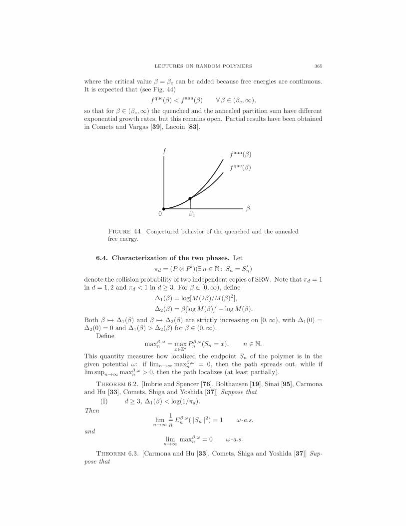
LECTURES ON RANDOM POLYMERS 365
where the critical value β = βc can be added because free energies are continuous.It is expected that (see Fig. 44)
fque(β) < fann(β) ∀β ∈ (βc,∞),
so that for β ∈ (βc,∞) the quenched and the annealed partition sum have differentexponential growth rates, but this remains open. Partial results have been obtainedin Comets and Vargas [39], Lacoin [83].
0β
f
fque(β)
fann(β)
βc
Figure 44. Conjectured behavior of the quenched and the annealedfree energy.
6.4. Characterization of the two phases. Let
πd = (P ⊗ P ′)(∃n ∈ N : Sn = S′n)
denote the collision probability of two independent copies of SRW. Note that πd = 1in d = 1, 2 and πd < 1 in d ≥ 3. For β ∈ [0,∞), define
∆1(β) = log[M(2β)/M(β)2],
∆2(β) = β[logM(β)]′ − logM(β).
Both β 7→ ∆1(β) and β 7→ ∆2(β) are strictly increasing on [0,∞), with ∆1(0) =∆2(0) = 0 and ∆1(β) > ∆2(β) for β ∈ (0,∞).
Definemaxβ,ωn = max
x∈ZdP β,ωn (Sn = x), n ∈ N.
This quantity measures how localized the endpoint Sn of the polymer is in thegiven potential ω: if limn→∞ maxβ,ωn = 0, then the path spreads out, while iflim supn→∞ maxβ,ωn > 0, then the path localizes (at least partially).
Theorem 6.2. [Imbrie and Spencer [76], Bolthausen [19], Sinai [95], Carmonaand Hu [33], Comets, Shiga and Yoshida [37]] Suppose that
(I) d ≥ 3, ∆1(β) < log(1/πd).
Then
limn→∞
1
nEβ,ωn (‖Sn‖2) = 1 ω-a.s.
andlimn→∞
maxβ,ωn = 0 ω-a.s.
Theorem 6.3. [Carmona and Hu [33], Comets, Shiga and Yoshida [37]] Sup-pose that
366 CARAVENNA, DEN HOLLANDER, AND PETRELIS
(II) d = 1, 2, β > 0 or d ≥ 3, ∆2(β) > log(2d).
Then there exists a c = c(d, β) > 0 such that
lim supn→∞
maxβ,ωn ≥ c ω-a.s.
Theorems 6.2–6.3 show that the polymer has qualitatively different behaviorin the two regimes. In (I), the scaling is diffusive, with the diffusion constantnot renormalized by the disorder. The reason why the diffusion constant is notrenormalized is the directedness of the path: this causes the annealed model tobe directed SRW. In (II), there is certainly no scaling to Brownian motion, dueto the presence of atoms: the endpoint of the polymer concentrates around oneor more most favorable sites whose locations depend on ω. These locations areexpected to be at a distance much larger than
√n, i.e., the scaling is predicted
to be superdiffusive. This has, however, only been proved in some special cases,in particular, for a one-dimensional model of a directed polymer in a Gaussianrandom environment (Petermann [88]). Further results, also for related models,have been obtained in Piza [92], Mejane [87], Carmona and Hu [34], Bezerra,Tindel and Viens [10] and Lacoin [85]. The latter reference contains a discussionof the physical conjectures and the mathematical results on this topic.
The proofs of Theorems 6.2–6.3 are based on a series of technical estimates forthe martingale (Y β,ωn )n∈N0
. These estimates also show that
(I) −→ (WD), (II) −→ (SD).
It has been conjectured that, throughout phase (SD),
Eβ,ωn (‖Sn‖2) ≍ n2ν n→ ∞, ω − a.s.
(≍ means modulo logarithmic factors), where the exponent ν is predicted not todepend on β and to satisfy
ν = 23 for d = 1, ν ∈ (12 ,
23 ) for d = 2,
signalling superdiffusive behavior.
6.5. Bounds on the critical temperature. Theorems 6.2–6.3 show thatβc = 0 for d = 1, 2 and βc ∈ (0,∞] for d ≥ 3 (because ∆1(0) = 0 and πd < 1).However, there is a gap between regimes (I) and (II) in d ≥ 3 (because πd > 1/2dand ∆1(β) > ∆2(β) for all β > 0). Thus, the results do not cover the full parameterregime. In fact, all we know is that
βc ∈ [β1c , β
2c ].
with (see Fig. 45)
β1c = sup
β ∈ [0,∞) : ∆1(β) < log(1/πd)
,
β2c = inf
β ∈ [0,∞) : ∆2(β) > log(2d)
.
Various attempts have been made to sharpen the estimates on βc: fractionalmoment estimates on the martingale (Evans and Derrida [52], Coyle [44], Camanesand Carmona [24]); size-biasing of the martingale (Birkner [11]). We describe thelatter estimate, which involves a critical threshold z∗ associated with the collisionlocal time of two independent SRWs.
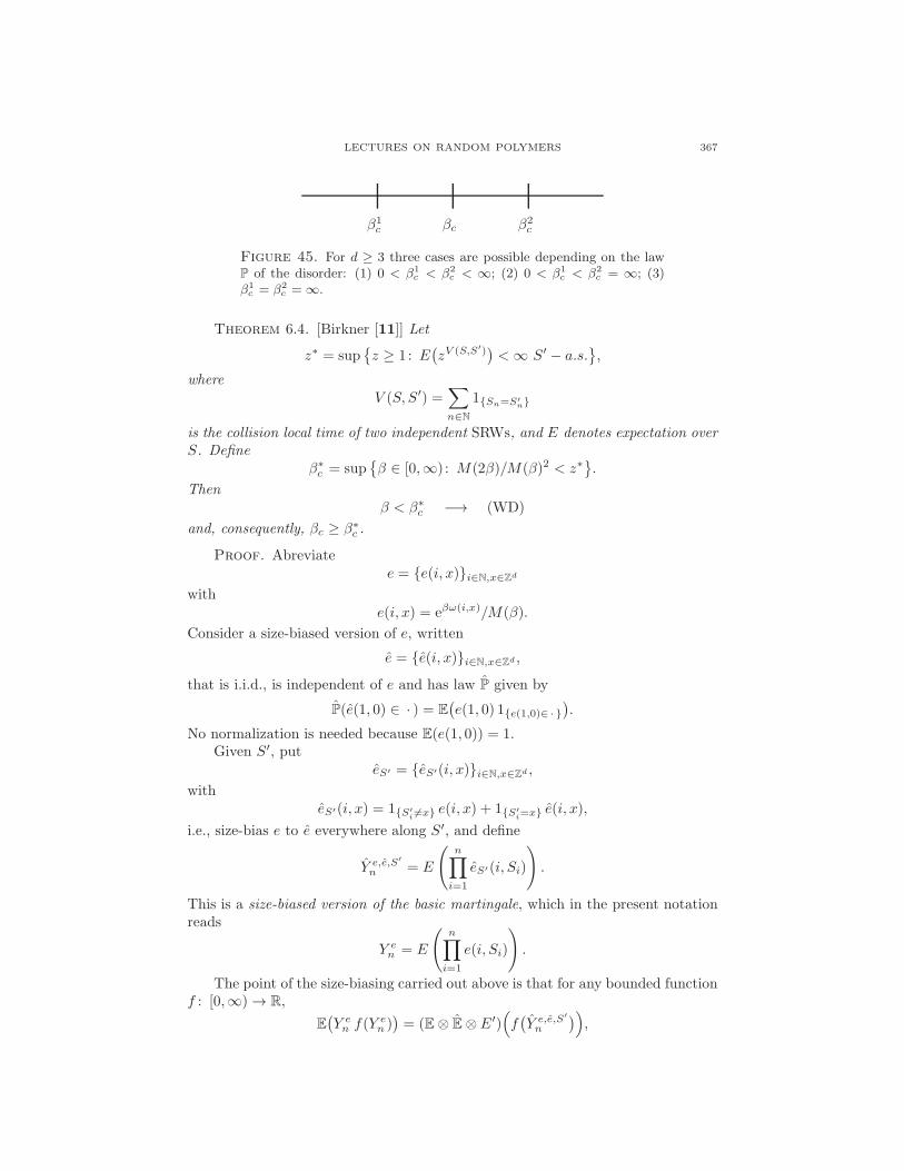
LECTURES ON RANDOM POLYMERS 367
βcβ1c β2
c
Figure 45. For d ≥ 3 three cases are possible depending on the lawP of the disorder: (1) 0 < β1
c < β2c < ∞; (2) 0 < β1
c < β2c = ∞; (3)
β1c = β2
c = ∞.
Theorem 6.4. [Birkner [11]] Let
z∗ = supz ≥ 1: E
(zV (S,S′)
)<∞ S′ − a.s.
,
whereV (S, S′) =
∑
n∈N
1Sn=S′n
is the collision local time of two independent SRWs, and E denotes expectation overS. Define
β∗c = sup
β ∈ [0,∞) : M(2β)/M(β)2 < z∗
.
Thenβ < β∗
c −→ (WD)
and, consequently, βc ≥ β∗c .
Proof. Abreviatee = e(i, x)i∈N,x∈Zd
withe(i, x) = eβω(i,x)/M(β).
Consider a size-biased version of e, written
e = e(i, x)i∈N,x∈Zd ,
that is i.i.d., is independent of e and has law P given by
P(e(1, 0) ∈ · ) = E(e(1, 0) 1e(1,0)∈ ·
).
No normalization is needed because E(e(1, 0)) = 1.Given S′, put
eS′ = eS′(i, x)i∈N,x∈Zd ,
witheS′(i, x) = 1S′
i 6=xe(i, x) + 1S′
i=xe(i, x),
i.e., size-bias e to e everywhere along S′, and define
Y e,e,S′
n = E
(n∏
i=1
eS′(i, Si)
).
This is a size-biased version of the basic martingale, which in the present notationreads
Y en = E
(n∏
i=1
e(i, Si)
).
The point of the size-biasing carried out above is that for any bounded functionf : [0,∞) → R,
E(Y en f(Y
en ))= (E⊗ E⊗ E′)
(f(Y e,e,S
′
n
)),

368 CARAVENNA, DEN HOLLANDER, AND PETRELIS
where E, E, E′ denote expectation w.r.t. e, e, S′, respectively. Indeed, the latterfollows from the computation
E(Y en f(Y
en ))= E
[E′
(n∏
i=1
e(i, S′i)
)f
(E
(n∏
i=1
e(i, Si)
))]
= E′
(E
[(n∏
i=1
e(i, S′i)
)f
(E
(n∏
i=1
e(i, Si)
))])
=! E′
((E⊗ E)
[f
(E
(n∏
i=1
eS′(i, Si)
))])
= (E⊗ E⊗ E′)(f(Y e,e,S
′
n
)),
where the third equality uses the definition of eS′ .The above identity relates the two martingales, and implies that
(Y en )n∈N0is uniformly integrable
⇐⇒ (Y e,e,S′
n )n∈N0is tight (∗)
(as can be seen by picking f such that limu→∞ f(u) = ∞). However, an easycomputation gives
(E⊗ E)(Y e,e,S
′
n
)= E
(z∑ni=1
1Si=S′i
)= E
(zV (S,S′)
)
with z = M(2β)/M(β)2, where the factor 2β arises because after the size-biasingthe intersection sites of S and S′ are visited by both paths. Hence
E(zV (S,S′)) <∞ S′-a.s.
is enough to ensure that the r.h.s. of (∗) holds. This completes the proof becausethe l.h.s. of (∗) is equivalent to (WD). Indeed, a.s. convergence plus uniform in-tegrability imply convergence in mean, so that E(Y en ) = 1 for all n ∈ N0 yieldsE(Y e) = 1.
In Birkner, Greven and den Hollander [13] it was proved that z∗ > πd in d ≥ 5,implying that β∗
c > β1c . It was conjectured that the same is true in d = 3, 4. Part of
this conjecture was settled in Birkner and Sun [14, 15] and Berger and Toninelli [9](see Fig. 46).
β1c β∗
c βc β2c
Figure 46. Bounds on the critical temperature.
6.6. Open problems.
• Show that in phase (SD) the polymer is concentrated inside a most favor-able corridor and identify how this corridor depends on ω.
• Determine whether βc is part of (WD) or (SD).• Derive a variational expression for βc.
LECTURES ON RANDOM POLYMERS 369
• Extend the analysis to undirected random walk. Important progress hasbeen made in Ioffe and Velenik [77, 78, 79, 80], Zygouras [104, 105],and references cited therein. See also Section 2.7.
Appendix A. Tutorial 1
In this tutorial we describe two methods that can be used to prove the existenceof the quenched free energy associated with the random pinning model describedin Section 4. Section A.1 recalls the model, Sections A.2–A.4 prove existence ofthe quenched free energy when the endpoint of the polymer is constrained to liein the interface, while Section A.5 shows how to remove this constraint afterwards.The method of proof is widely applicable, and is not specific to the random pinningmodel.
A.1. Random pinning of a polymer at an interface. Configurations ofthe polymer. Let n ∈ N and consider a polymer made of n monomers. The al-lowed configurations of this polymer are modeled by the n-step trajectories of a1-dimensional random walk S = (Si)i∈N0
. We focus on the case where S0 = 0 and(Si − Si−1)i∈N is an i.i.d. sequence of random variables satisfying
P (S1 = 1) = P (S1 = −1) = P (S1 = 0) = 13 ,
although the argument given below applies more generally. We denote by Wn theset of all n-step trajectories of S.
Disorder at interface. Let ω = (ωi)i∈N be an i.i.d. sequence of R-valued randomvariables (which we take bounded for ease of exposition). For i ∈ N the interactionintensity between the i-th monomer and the interface takes the value ωi. Note thatω and S are independent, and write P for the law of ω. Pick M > 0 such that|ω1| ≤M P-a.s.
Interaction polymer-interface. The flat interface that interacts with the polymer islocated at height 0, so that the polymer hits this interface every time S comes backto 0. Thus, with every S ∈ Wn we associate the energy
Hβ,ωn (S) = −β
n−1∑
i=0
ωi 1Si=0,
where β ∈ (0,∞) stands for the inverse temperature (and for ease of exposition wetake zero bias, i.e., we set h = 0 in the Hamiltonian in Section 4.1). We think of Sas a random realization of the path of the polymer.
Partition function and free energy. For fixed n, the quenched (= frozen disorder)partition function and free energy are defined as
Zβ,ωn = E(e−H
β,ω
N(S))
and fβ,ωn = 1n logZω,βn .
A.2. Convergence of the free energy. Our goal is to prove the followingtheorem.
Theorem A.1. For every β ∈ R there exists an f(β) ∈ [0, βM ] such that
limn→∞
E(fβ,ωn ) = f(β)
andlimn→∞
fβ,ωn = f(β) P− a.e. ω.
370 CARAVENNA, DEN HOLLANDER, AND PETRELIS
As indicated above, we will prove Theorem A.1 via two different methods. InSection A.3 we will state Kingman’s Subadditive Ergodic Theorem and see how thiscan be applied to obtain Theorem A.1. In Section A.4 we will re-prove Theorem A.1by using a concentration of measure argument. The latter method is more involved,but also more flexible than the former method. For technical reasons, we will firstprove Theorem A.1 with the partition function restricted to those trajectories thathit the interface at their right extremity, i.e.,
Z∗,β,ωn = E
(e−H
β,ωn (S) 1Sn=0
)and f∗,β,ω
n = 1n logZ∗,β,ω
n .
In Section A.5 we will see that the restriction on the endpoint has no effect on thevalue of the limiting free energy.
A.3. Method 1: Kingman’s theorem.
Theorem A.2. [Kingman’s Subadditive Ergodic Theorem; see Steele [98]] Let(Ω, A, µ) be a probability space, let T be an ergodic measure-preserving transforma-tion acting on Ω, and let (gn)n∈N be a sequence of random variables in L1(µ) thatsatisfy the subadditivity relation
gm+n ≥ gm + gn(Tm), m, n ∈ N.
Thenlimn→∞
gnn
= supk∈N
Eµ
(gkk
)µ-a.s.
(1) Let T be the left-shift on RN. Prove that, for m,n ∈ N and ω ∈ R
N,
logZ∗,β,ωm+n ≥ logZ∗,β,ω
m + logZ∗,β,Tm(ω)n .
(2) Apply Theorem A.2 with (Ω, A, µ) = (RN,Bor(RN),P) and prove Theorem A.1with the endpoint restriction.
A.4. Method 2: Concentration of measure. This method consists of firstproving the first line in Theorem A.1, i.e., the convergence of the average quenchedfree energy, and then using a concentration of measure inequality to show that,with large probability, the quenched free energy is almost equal to its expectation,so that the second line in Theorem A.1 follows. See Giacomin and Toninelli [58]for fine details.
(1) Use (A.3) and prove that (E(logZ∗,β,ωn ))n∈N is a superadditive sequence, i.e.,
for m,n ∈ N,
E(logZ∗,β,ωm+n ) ≥ E(logZ∗,β,ω
m ) + E(logZ∗,β,ωn ).
(2) Deduce that (see also the tutorial in Appendix A.1 of Bauerschmidt, Duminil-Copin, Goodman and Slade [7])
limn→∞
E(f∗,β,ωn ) = sup
k∈N
E(f∗,β,ωk ) = f(β) ∈ [0, βM ].
To proceed, we need the following inequality.
Theorem A.3. [Concentration of measure; see Ledoux [86]] There exist C1, C2
> 0 such that for all n ∈ N, K > 0, ε > 0 and Gn : Rn 7→ R a K-Lipschitz (w.r.t.
the Euclidean norm) convex function,
P
(∣∣Gn(ω0, . . . , ωn−1)− E(Gn(ω0, . . . , ωn−1)
)∣∣ > ε)≤ C1e
−C2ε
2
K2 .
LECTURES ON RANDOM POLYMERS 371
(3) By Holder’s inequality, the function ω ∈ Rn 7→ f∗,β,ω
n ∈ R is convex. To provethat it is (β/
√n)-Lipschitz, pick ω, ω′ ∈ R
n and compute
∣∣∣∣∂
∂tf∗,β,tω+(1−t)ω′
n
∣∣∣∣ =β
n
∣∣∣∣∣
n−1∑
i=0
P ∗,β,ωn (Si = 0) (ωi − ω′
i)
∣∣∣∣∣
≤ β
n
√√√√n−1∑
i=0
[P ∗,β,ωn (Si = 0)
]2√√√√
n−1∑
i=0
(ωi − ω′i)
2
≤ β√n
√√√√n−1∑
i=0
(ωi − ω′i)
2,
where P ∗,β,ωn is the path measure with the endpoint restriction.
(4) Apply Theorem A.3 to prove that, for ε > 0,
∑
n∈N
P(|f∗,β,ωn − E(f∗,β,ω
n )| > ε)<∞.
(5) Combine (2) and (4) to show that, for P-a.e. ω, f∗,β,ωn tends to f(β) as n→ ∞,
which proves Theorem A.1 with the endpoint restriction.
A.5. Removal of the path restriction. The proof of Theorem A.1 will becompleted once we show that restricting the partition function to Sn = 0 doesnot alter the results. To that end, we denote by τ the first time at which therandom walk S hits the interface.
(6) Note that there exists a C3 > 0 such that (see Spitzer [97], Section 1)
P (τ = n) =C3
n3/2[1 + o(1)] and P (τ > n) =
2C3
n1/2[1 + o(1)].
(7) Consider the last hit of the interface and show that
Zβ,ωn =n∑
j=0
Z∗,β,ωj P (τ > n− j).
(8) Prove Theorem A.1 by combining (5), (6) and (7).
Appendix B. Tutorial 2
The goal of this tutorial is to provide the combinatorial computation of the freeenergy for the directed polymer with self-attraction described in Sections 2.4–2.5leading to Theorem 2.3. This computation is taken from Brak, Guttmann andWhittington [23]. Section B.1 recalls the model, Section B.2 proves the existenceof the free energy, while Section B.3 derives a formula for the free energy with thehelp of generating functions.

372 CARAVENNA, DEN HOLLANDER, AND PETRELIS
B.1. Model of a directed polymer in a poor solvent. We begin by re-calling some of the notation used in Sections 2.4–2.5.
Configurations of the polymer. For n ∈ N, the configurations of the polymer aremodelled by n-step (1 + 1)-dimensional directed self-avoiding paths w = (wi)
ni=0
that are allowed to move up, down and to the right, i.e.,
Wn = (wi)ni=0 ∈ (N0 × Z)n+1 : w0 = 0, w1 − w0 =→,
wi − wi−1 = ↑, ↓,→ ∀1 ≤ i ≤ n,
wi 6= wj ∀ 0 ≤ i < j ≤ n.
Self-touchings. The monomers constituting the polymer have an attractive interac-tion: an energetic reward is given for each self-touching, i.e., for each pair (wi, wj)with i < j − 1 and |wi −wj | = 1. Accordingly, with each w ∈ Wn we associate thenumber of self-touchings
Jn(w) =∑
0≤i<j−1≤n−1
1|wi−wj |=1,
and the energyHγn(w) = −γJn(w),
where γ ∈ R is the interaction parameter.
Partition function, free energy and generating function. For fixed n, the partitionfunction and free energy are defined as
Zγn =∑
w∈Wn
e−Hγn(w), fn(γ) =
1n logZγn .
For n ∈ N0 and x ∈ [0,∞), let
Zn(x) =∑
m∈N0
cn(m)xm, cn(m) = |w ∈ Wn : Jn(w) = m|.
Then Zγn = Zn(eγ), and the generating function of Zγn can be written as
∑
n∈N0
Zγnyn = G(eγ , y)
withG(x, y) =
∑
n∈N0
∑
m∈N0
cn(m)xmyn, x, y ∈ [0,∞).
B.2. Existence of the free energy. Existence comes in three steps.
(1) Show that for m,n ∈ N0 and x ∈ [0,∞),
Zm+n+1(x) ≥ Zm(x)Zn(x) and Zn(x) ≤ [3(1 ∨ x)]n.
(2) Deduce that
limn→∞
1
nlogZn(x) = sup
k∈N
1
klogZk(x) = f(x) ∈ (0, log 3 + (0 ∨ log x)].
Thus, f(γ) = f(eγ), γ ∈ R.
(3) For x ∈ [0,∞), let yc(x) be the radius of convergence of the generating functionG(x, y). Show that
(B.1) f(x) = − log yc(x).
LECTURES ON RANDOM POLYMERS 373
B.3. Computation of the free energy. To prove Theorem 2.3, we mustcompute yc(x), x ∈ [0,∞). In what follows we derive the formula for G(x, y) givenin Lemma 2.4.
(1) For n, r, s ∈ N0, let
Wn,r
= w ∈ Wn : w makes exactly r vertical steps after the first step east,Wn,r,s
= w ∈ Wn,r : w makes exactly s vertical steps after the second step east,
and note that Wn,r = ∅ if n < 1 + r and Wn,r,s = ∅ if n < 2 + r + s. Furthermore,for r, s ∈ N, let
W ↑↓n,r,s
= w ∈ Wn,r,s : the r and s vertical steps are made in opposite directions,W ↑↑n,r,s
= w ∈ Wn,r,s : the r and s vertical steps are made in the same direction,
so that, for r ∈ N, Wn,r can be partitioned as
Wn,r =
n−r−2⋃
s=0
Wn,r,s = Wn,r,0 ∪[n−r−2⋃
s=1
[W ↑↓n,r,s ∪W ↑↑
n,r,s
]].
For n, r,m ∈ N0, let cn,r(m) be the number of n-step paths with m self-touchingsmaking exactly r steps north or south immediately after the first step east, and put
gr(x, y) =∑
n∈N0
∑
m∈N0
cn,r(m)xm yn.
Clearly, G(x, y) =∑r∈N0
gr(x, y).
(2) Pick r ∈ N and use the first equality in the partitioning of Wn,r, together withthe fact that cn,r(m) = 0 when n < r + 1, to prove that
gr(x, y) = 2yr+1 +∑
s∈N0
∞∑
n=r+2+s
∑
w∈Wn,r,s
xJn(w) yn.
For w ∈ Wn and 0 ≤ l < s ≤ n, let
Jl,s(w) =∑
l≤i<j−1≤s−1
1|wi−wj |=1,
which stands for the number of self-touchings made by w between its l-th and s-thstep. Clearly, Jn(w) = J0,n(w).
(3) Pick r, s ∈ N and n ≥ r + s+ 2. Prove that
w ∈ W ↑↑n,r,s −→ Jn(w) = Jr+1,n(w),
w ∈ W ↑↓n,r,s −→ Jn(w) = Jr+1,n(w) + minr, s.
374 CARAVENNA, DEN HOLLANDER, AND PETRELIS
(4) Use (2) and (3) to show that
gr(x, y) = yr+1
[2 +
r∑
s=0
(1 + xs) gs(x, y) +∞∑
s=r+1
(1 + xr) gs(x, y)
], r ∈ N.
(B.2)
In the same spirit show that
(B.3) g0(x, y) = y + y G(x, y).
(5) Abbreviate gr = gr(x, y). Prove that
(B.4) gr+1 − (1 + x)ygr − (1 − x)xryr+2gr + xy2gr−1 = 0 r ∈ N.
To do so, substitute the expressions obtained for gr−1, gr and gr+1 from (B.2) into(B.4), and isolate the terms containing y2r+3. The latter leads to a rewrite of theleft-hand side of (B.4) as
(B.5) xry2r+3(x− 1)
[2 +
r∑
s=0
(1 + xs)gs +
∞∑
s=r+1
(1 + xr)gs
]+ xryr+2(1− x)gr.
Use (B.2) once more to conclude that (B.5) equals zero.
(6) From (B.4) we see that (gr)r∈N0is determined by g0 and g1, while (B.3) con-
stitutes a consistency relation that must be met by the solution of (B.4). Thus,(gr)r∈N0
belongs to a two-dimensional vector space generated by any two linearlyindependent solutions. For this reason, we look for two particular solutions of (B.4)by making an Ansatz. Set q = xy, and write gr in the form
(B.6) gr = λr∑
l∈N0
pl qlr, r ∈ N, p0 = 1,
where λ = λ(y, q) and pl = pl(λ, y, q), l ∈ N, are to be determined. Substitute (B.6)into (B.4) to obtain
(B.7)
λ2 − λ(y + q) + yq
+∑
l∈N
ql(r−1)[(λ2q2l − λ(y + q)ql + yq
)pl +
(λ(q − y)yql
)pl−1
]= 0.
Conclude that (B.7) is satisfied when
(B.8) pl =λ(y − q)yql
(λql − y)(λql − q)pl−1, l ∈ N,
provided λ solves the equation λ2 − λ(y + q) + yq = 0, i.e., λ ∈ λ1, λ2 = y, q.(7) Use (6) to show that gr = C1gr,1+C2gr,2, r ∈ N, where C1 and C2 are functionsof y, q and(B.9)
gr,i = gr,i(x, y) = (λi)r
(1+∑
k∈N
(λi)k(y − q)kykq
12k(k+1)
∏kl=1(λiq
l − y)(λiql − q)qkr)
i = 1, 2, r ∈ N0.
Pick x > 1 and 0 < y < 1 such that q = xy < 1, and let r → ∞ in (B.9). This gives
limr→∞
q−rgr,1(x, y) = 0 and limr→∞
q−rgr,2(x, y) = 1.
LECTURES ON RANDOM POLYMERS 375
Next, an easy computation shows that limr→∞1r log |Wr| = 1 +
√2, with |Wr| =
gr(1, 1). Pick x > 1 and 0 < y < 1 such that q = xy < 1/(1 +√2), and let r → ∞
in (B.2). This gives
limr→∞
q−rgr(x, y) = 0,
from which it follows that C2 = 0.
(8) It remains to determine C1. To that end, note that, by construction, (gr,1)r∈N0
satisfies (B.4) for r = 0 as well. Use (B.3) and (B.4) to show that
(B.10)12C1g0,1 = g0 = y + yG,
C1g1,1 = g1 = a+ bG,
with
a = y2(2 + y − xy), b = y2(1 + x+ y − xy).
Eliminate C1 and express G in terms of g0,1 and g1,1, to obtain
G(x, y) =aH(x, y)− y2
bH(x, y)− y2,
where
H(x, y) = yg0,1(x, y)
g1,1(x, y).
This completes the proof of Lemma 2.4 with g0 = g0,1 and g1 = g1,1.
(9) Brak, Guttmann and Whittington [23] show that the function H(x, y) can berepresented as a continued fraction. This representation allows for an analysis ofthe singularity structure of G(x, y), in particular, for a computation of yc(x) (theradius of convergence of the power series y 7→ G(x, y)) for fixed x. For instance,from (B.4) it is easily deduced that
G(1/y, y) =∑
r∈N0
gr(1/y, y) = −1 +
√1− y
1− 3y − y2 − y3(q = 1)
and this has a singularity at yc solving the cubic equation 1 − 3y − y2 − y3 = 0.Fig. 16 gives the plot of x 7→ yc(x) that comes out of the singularity analysis. Asexplained in Section B.3, the free energy is f(γ) = − log yc(e
γ).
Appendix C. Tutorial 3
The purpose of this tutorial is to take a closer look at the free energy of thehomogeneous pinning model described in Section 3. Section C.1 recalls the model,Section C.2 computes the free energy, while Section C.3 identifies the order of thephase transition.
C.1. The model. Let (Sn)n∈N0be a random walk on Z, i.e., S0 = 0 and
Si − Si−1, i ∈ N, are i.i.d. Let P denote the law of S. Introducing the first returntime to zero τ = infn ∈ N : Sn = 0, we denote by R(·) its distribution:
R(n) = P (τ = n) = P(Si 6= 0 ∀ 1 ≤ i ≤ n− 1, Sn = 0
), n ∈ N.
We require that∑
n∈NR(n) = 1, i.e., the random walk is recurrent, and we assume
the following tail asymptotics for R(·) as n→ ∞:
R(n) =c
n1+a[1 + o(1)], c > 0, a ∈ (0, 1) ∪ (1,∞).
376 CARAVENNA, DEN HOLLANDER, AND PETRELIS
The exclusion of a = 1 is for simplicity (to avoid logarithmic corrections in laterstatements). The constant c could be replaced by a slowly varying function atthe expense of more technicalities, which however we avoid. We recall that, for anearest-neighbor symmetric random walk, i.e., when P (S1 = 1) = P (S1 = −1) = pand P (S1 = 0) = 1 − 2p with p ∈ (0, 12 ), the above tail asymptotics holds with
α = 12 .The set of allowed polymer configurations is Wn = w = (i, wi)
ni=0 : w0 =
0, wi ∈ Z ∀ 0 ≤ i ≤ n, on which we define the Hamiltonian Hζn(w) = −ζLn(w),
where ζ ∈ R and
Ln(w) =n∑
i=1
1wi=0, w ∈ Wn,
is the so-called local time of the polymer at the interface (which has height zero).We denote by Pn the projection of P ontoWn, i.e., Pn(w) = P (Si = wi ∀ 1 ≤ i ≤ n)for w ∈ Wn. This is the a priori law for the non-interacting polymer. We defineour polymer model as the law P ζn on Wn given by
P ζn(w) =1
Zζne−H
ζn(w) Pn(w), w ∈ Wn.
The normalizing constant Zζn, called the partition function, is given by
Zζn =∑
w∈Wn
e−Hζn(w) Pn(w) = En
(e−H
ζn(w)
)= E
(eζ
∑ni=1 1Si=0
).
The free energy f(ζ) is defined as the limit
f(ζ) = limn→∞
1
nlogZζn,
which has been shown to exist in Tutorial 1. From a technical viewpoint it is moreconvenient to consider the constrained partition sum Z∗,ζ
n defined by
Z∗,ζn =
∑
w∈Wnwn=0
e−Hζn(w) Pn(w) = E
(eζ
∑ni=1
1Si=0 1Sn=0
).
As shown in Tutorial 1, if we replace Zζn by Z∗,ζn in the definition of f(ζ), then
this does not change the value of the limit. Therefore we may focus on Z∗,ζn .
C.2. Computation of the free energy. We repeat in more detail the deriva-tion of the formula for the free energy f(ζ) given in Section 3.
(1) Prove that Z∗,ζn ≥ eζ P (τ = n) = eζ R(n). Deduce that f(ζ) ≥ 0 for every
ζ ∈ R.(2) Show that Z∗,ζ
n ≤ 1 for ζ ∈ (−∞, 0]. Deduce that f(ζ) = 0 for everyζ ∈ (−∞, 0].
(3) Henceforth we focus on ζ ∈ [0,∞). Define for x ∈ [0, 1] the generatingfunction φ(x) =
∑n∈N
R(n)xn. Observe that x 7→ φ(x) is strictly in-creasing with φ(0) = 0 and φ(1) = 1. Deduce that for every ζ ∈ [0,∞)there is exactly one value r = r(ζ) that solves the equation φ(e−r) = e−ζ .
Observe that Rζ(n) = eζ R(n) e−r(ζ)n defines a probability distributionon N.

LECTURES ON RANDOM POLYMERS 377
(4) For n ∈ N and 1 ≤ k ≤ n, denote by Θn,k the set consisting of k+1 pointsdrawn from the interval 0, . . . , n, including 0 and n. More explicitly, theelements of Θn,k are of the form j = (j0, j1, . . . , jk) with j0 = 0, jk = nand ji−1 < ji for all 1 ≤ i ≤ n. By summing over the locations i at whichSi = 0, prove that
Z∗,ζn =
n∑
k=1
eζk∑
j∈Θn,k
k∏
i=1
R(ji − ji−1).
Note that this equation can be rewritten as
Z∗,ζn = er(ζ)n uζ(n), uζ(n) =
n∑
k=1
∑
j∈Θn,k
k∏
i=1
Rζ(ji − ji−1).
(5) For fixed ζ ∈ (0,∞), we introduce a renewal process (τn)n∈N0with law
Pζ , which is a random walk on N0 with positive increments, i.e., τ0 = 0
and τn − τn−1, n ∈ N, are i.i.d. under Pζ with law Pζ(τ1 = n) = Rζ(n).Show that the following representation formula holds:
uζ(n) =
n∑
k=1
Pζ(τk = n) = Pζ
(⋃
k∈N
τk = n).
In particular, uζ(n) ≤ 1. We will use the following important result knownas the renewal theorem:
limn→∞
uζ(n) = C ∈ (0,∞).
Here C = C(ζ) = [∑
m∈NmRζ(m)]−1 ∈ (0,∞).
(6) Conclude that limn→∞1n logZ∗,ζ
n = r(ζ) for every ζ ∈ [0,∞). This meansthat for ζ ∈ [0,∞) the free energy f(ζ) coincides with r(ζ) and thereforesatisfies the equation φ(e−f(ζ)) = e−ζ .
Note that (4) and (5) give a sharp asymptotics of the constrained partition sum.Also note that the argument only uses the renewal structure of the excursions ofthe polymer away from the interface, and therefore can be extended to deal with apriori random processes other than random walks.
C.3. Order of the phase transition. From the relation φ(e−f(ζ)) = e−ζ wenext derive some interesting properties of the free energy.
(1) Observe that for x ∈ (0, 1) the function φ(x) =∑n∈N
R(n)xn is strictlyincreasing, with non-vanishing first derivative, and is real analytic. Sinceφ(0) = 0 and φ(1) = 1, its inverse φ−1, defined from (0, 1) onto (0, 1),is real analytic too, by the Lagrange inversion theorem. Deduce that thefree energy ζ 7→ f(ζ) = − logφ−1(e−ζ) restricted to ζ ∈ (0,∞) is realanalytic. The same is trivially true for ζ ∈ (−∞, 0), since f(ζ) = 0.
(2) Conclude that the free energy ζ 7→ f(ζ) is not analytic at ζ = 0, by theidentity theorem of analytic functions. Observe that nevertheless the freeenergy is continuous at ζ = 0.
(3) Introduce the integrated tail probability R(n) =∑∞
k=n+1R(k) for n ∈ N0.
Deduce from our tail assumption on R(·) that R(n) = can
−a[1 + o(1)] asn→ ∞.

378 CARAVENNA, DEN HOLLANDER, AND PETRELIS
(4) Use summation by parts to show that 1 − φ(x) = (1 − x)∑
n∈N0R(n)xn
for x ∈ (0, 1).
Proof.
1− φ(x) = 1−∑
n∈N
R(n)xn = 1−∑
n∈N
(R(n− 1)−R(n))xn
=
(1 +
∑
n∈N
R(n)xn
)−∑
n∈N
R(n− 1)xn =∑
n∈N0
R(n)xn −∑
n∈N0
R(n)xn+1
= (1− x)∑
n∈N0
R(n)xn.
(5) Put ψ(x) =∑
n∈N0R(n)xn, so that 1−φ(x) = (1−x)ψ(x). We first focus
on a ∈ (1,∞). Show that in that case ψ(1) = E(τ) =∑
n∈NnR(n) ∈
(0,∞). Deduce from φ(e−f(ζ)) = e−ζ that, as ζ ↓ 0,
f(ζ) =1
E(τ)ζ [1 + o(1)], a ∈ (1,∞).
(6) We next focus on a ∈ (0, 1). Use a Riemann sum approximation to showthat, as r ↓ 0,
ψ(e−r) =
(cΓ(1− a)
a
)ra−1 [1 + o(1)],
where
Γ(1− a) =
∫ ∞
0
e−t
tadt ∈ (0,∞).
Proof. Note that, for a ∈ (0, 1), ψ(e−r) ↑ ∞ as r ↓ 0, becauseR(n) = c
an−a [1 + o(1)]. Therefore, for any fixed n0 ∈ N, we can safely
neglect the first n0 terms in the sum defining ψ(·), because they give afinite contribution as r ↓ 0. This gives
ψ(e−r) ∼∞∑
n=n0
R(n)e−nr ∼ c
a
∞∑
n=n0
e−nr
na=c
ara−1
∞∑
n=n0
re−nr
(nr)a
∼ c
ara−1
(∫ ∞
0
e−t
tadt
),
where ∼ refers to n0 → ∞.
(7) Deduce from φ(e−f(ζ)) = e−ζ that, as ζ ↓ 0,
f(ζ) =
(a
cΓ(1− a)
)1/a
ζ1/a [1 + o(1)], a ∈ (0, 1).
Note that the smaller a is, the more regular is the free energy for ζ ↓ 0, i.e., thehigher is the order of the phase transition at ζ = 0. For a ∈ (1,∞) the derivative ofthe free energy is discontinuous at ζ = 0, which corresponds to a first-order phasetransition.
LECTURES ON RANDOM POLYMERS 379
Appendix D. Tutorial 4
The purpose of this (long) tutorial is to provide further detail on the variationalapproach to the random pinning model described in Section 4. Section D.1 recallsthe model, Section D.2 provides the necessary background on large deviation theory,Section D.3 explains the large deviation principles for the empirical process ofrandom words cut out from a random letter sequence according to a renewal process,while Section D.4 shows how the latter are applied to the random pinning modelto derive a variational formula for the critical curve.
D.1. The model. Let S = (Sn)n∈N0, be a Markov chain on a countable space
Υ that contains a marked point ∗. Let P denote the law of S, and assume thatS0 = ∗. We introduce the first return time to ∗, namely, τ = infn ∈ N : Sn = ∗,and we denote by R(·) its distribution:
R(n) = P (τ = n) = P (Si 6= ∗ ∀ 1 ≤ i ≤ n− 1, Sn = ∗), n ∈ N.
We require that∑
n∈NR(n) = 1, i.e., the Markov chain is recurrent, and assume
the following logarithmic tail asymptotics as n→ ∞:
limn→∞
logR(n)
logn= −(1 + a) , with a ∈ [0,∞) .
For a nearest-neighbor and symmetric random walk on Z, i.e.,
P (S1 = 1) = P (S1 = −1) = p, P (S1 = 0) = 1− 2p, p ∈ (0,1
2),
this asympotics holds with a = 12 .
The set of allowed polymer configurations is Wn = w = (i, wi)ni=0 : w0 =
∗, wi ∈ Υ ∀ 0 < i ≤ n on which we define the Hamiltonian
Hβ,h,ωn (w) = −
n∑
i=0
(βωi − h)1wi=∗,
where β, h ≥ 0 are two parameters that tune the interaction strength and ω =(ωi)i∈N0
is the random environment, a typical realization of a sequence of i.i.d. R-valued random variables with marginal law µ0. The law of the full sequence ω istherefore P = µ⊗N0
0 . We assume that M(β) = E(eβω0) < ∞ for all β ∈ R, andw.l.o.g. we assume that E(ω0) = 0 and E(ω2
0) = 1.We denote by Pn the projection onto Wn of the law of S, i.e., Pn(w) = P (Si =
wi ∀ 0 ≤ i ≤ n) for w ∈ Wn. This is the a priori law for the non-interactingpolymer. We define our polymer model as the law P β,h,ωn on Wn given by
P β,h,ωn (w) =1
Zβ,h,ωn
e−Hβ,h,ωn (w) Pn(w).
The normalizing constant Zβ,h,ωn is the partition sum and is given by
Zβ,h,ωn =∑
w∈Wn
e−Hβ,h,ωn (w) Pn(w)
= En
(e−H
β,h,ωn (w)
)= E
(e∑ni=0
(βωi−h)1wi=∗
).D
The quenched free energy fque(β, h) is defined as the limit
fque(β, h) = limn→∞
1
nlogZβ,h,ωn P-a.s. and in L1(P),
380 CARAVENNA, DEN HOLLANDER, AND PETRELIS
which has been shown in Tutorial 1 to exist and to be non-random. It can be easilyshown that fque(β, h) ≥ 0, which motivates the introduction of a localized phase Land a delocalized phase D defined by
L = (β, h) : fque(β, h) > 0, D = (β, h) : fque(β, h) = 0.
It follows from the convexity and the monotonicity of the free energy that thesephases are separated by a quenched critical curve
β 7→ hquec (β) = infh ∈ R : fque(β, h) = 0.
In the remainder of this tutorial we develop insight into the variational formula forhquec that was put forward in Section 5.
Note that fque(β, h) = limn→∞1nE(logZn(β, h, ω)). Interchanging the expec-
tation E and the logarithm, we obtain the annealed free energy:
fann(β, h) = limn→∞
1
nlogE
(Zβ,h,ωn
)= lim
n→∞
1
nlogE
(e(logM(β)−h)
∑ni=0
1Si=∗),
which is nothing but the free energy f(ζ) of a homogeneous pinning model withζ = logM(β)− h. Recall from Tutorial 3 that f(ζ) > 0 for ζ > 0 and f(ζ) = 0 forζ ≤ 0. Introducing the annealed critical curve
hannc (β) = infh ∈ R : fann(β, h) = 0,
we find that hannc (β) = logM(β). Jensen’s inequality yields fque(β, h) ≤ fann(β, h),so that hquec (β) ≤ hannc (β). The disorder is said to be irrelevant if hquec (β) = hannc (β)and relevant if hquec (β) < hannc (β).
D.2. Some background on large deviation theory. Before we proceedwith our analysis of the copolymer model we make an intermezzo, namely, we givea brief summary of some basic large deviation results. For more details, see themonographs by Dembo and Zeitouni [47] and den Hollander [69].
D.2.1. Relative entropy. Let ν, ρ be two probabilities on a measurable space(Γ,G), i.e., ν, ρ ∈ M1(Γ), the space of probability measures on Γ. For ν ≪ ρ (i.e.,ν is absolutely continuous with respect to ρ), we denote by dν
dρ the corresponding
Radon-Nikodym derivative and we define the relative entropy h(ν|ρ) of ν withrespect to ρ by the formula
h(ν|ρ) =∫
Γ
log
(dν
dρ
)dν =
∫
Γ
(dν
dρ
)log
(dν
dρ
)dρ.
For ν 6≪ ρ, we simply put h(ν|ρ) = ∞. Note that the function g(x) = x log x withg(0) = 0 is convex (hence continuous) and is bounded from below on [0,∞), so thatthe integral defining h(ν|ρ) is well-defined in R ∪ ∞.
• Use Jensen’s inequality to show that h(ν|ρ) ≥ 0 for all ν, ρ, with h(ν|ρ) = 0if and only if ν = ρ.
For fixed ρ, the function ν 7→ h(ν|ρ) is convex on M1(Γ). Note that if Γ is afinite set, say Γ = 1, . . . , r with r ∈ N, then we can write
h(ν|ρ) =r∑
i=1
νi log
(νiρi
).
LECTURES ON RANDOM POLYMERS 381
D.2.2. Sanov’s Theorem in a finite space. Let Y = (Yn)n∈N be an i.i.d. se-quence of random variables taking values in a finite set, which we identify withΓ = 1, . . . , r with r ∈ N. Let ρ = ρiri=1 with ρi = P (Y1 = i) > 0 be themarginal law of this random sequence. Note that ρ ∈ M1(Γ). For n ∈ N we definethe empirical measure
Ln =1
n
n∑
k=1
δYk ,
where δx denotes the Dirac mass at x. Note that Ln is a random element ofM1(Γ), i.e., a random variable taking values in M1(Γ), which describes the relativefrequency of the “letters” appearing in the sequence Y1, . . . , Yn.
The space M1(Γ) can be identified with the simplex x ∈ (R+)r :∑ri=1 xi =
1 ⊂ (R+)r, and hence M1(Γ) can be equipped with the standard Euclidean topol-ogy, and we can talk about convergence in M1(Γ) (which is nothing but conver-gence of every component). With this identification we have Ln = Ln(i)ri=1,where Ln(i) is the relative frequency of the symbol i in the sequence Y1, . . . , Yn,i.e., Ln(i) =
1n
∑nk=1 1Yk=i.
• Show that the strong law of large numbers yields the a.s. convergencelimn→∞ Ln = ρ, where the limit is in M1(Γ).
The purpose of large deviation theory is to quantify the probability that Lndiffers from its limit ρ: given a ν ∈ M1(Γ) different from µ, what is the probability
that Ln is close to ν? Take for simplicity ν = νiri=1 of the form νi =kin with
ki ∈ N and∑r
i=1 ki = n. (Note that this is the family of laws that can be attainedby Ln.)
• Prove that P (Ln = ν) = n!∏ri=1
ρiki
ki!.
• Use Stirling’s formula n! = nne−n+o(n) to deduce that P (Ln = ν) =e−nh(ν|ρ)+o(n), where h(ν|ρ) is the relative entropy defined above.
In this sense, the relative entropy h(ν|ρ) gives the rate of exponential decay forthe probability that Ln is close to ν instead of ρ. More generally, it can be shownthat if O and C are, respectively, an open and a closed subset of M1(Γ), then, withthe notation I(ν) = h(ν|ρ), the following relations hold:
(D.1)
lim infn→∞
1
nlogP (Ln ∈ O) ≥ − inf
ν∈OI(ν),
lim supn→∞
1
nlogP (Ln ∈ C) ≤ − inf
ν∈CI(ν).
Whenever the above inequalities hold, we say that the sequence of random variables(Ln)n∈N satisfies the large deviation principle (LDP) with rate n and with ratefunction I(·).
D.2.3. Sanov’s theorem in a Polish space. In the previous section we haveworked under the assumption that the space Γ is finite. However, everything canbe generalized to the case when Γ is Polish (a complete separable metric space)equipped with the Borel σ-field. Let Y = (Yn)n∈N be an i.i.d. sequence of randomvariables taking values in Γ and denote by ρ ∈ M1(Γ) the law of Y1. We equip thespace M1(Γ) of probability measures on Γ with the topology of weak convergence(i.e., νn → ν in M1(Γ) if and only if
∫fdνn →
∫fdν for every bounded and con-
tinuous f : Γ → R). This topology turns M1(Γ) into a Polish space too, which weequip with the corresponding Borel σ-field. We can therefore speak of convergence
382 CARAVENNA, DEN HOLLANDER, AND PETRELIS
in M1(Γ) as well as random elements of M1(Γ) (random variables taking values inM1(Γ)).
In particular, the empirical measure Ln introduced above is well defined inthis generalized setting as a random element of M1(Γ). With the help of theergodic theorem it is possible to show that, in analogy with the case of finite Γ,limn→∞ Ln = ρ a.s. in M1(Γ). Also, the large deviation inequalities mentionedabove continue to hold, again with I(ν) = h(ν|ρ) as defined earlier. The formaltool to prove this is the projective limit LDP of Dawson and Gartner [46].
D.2.4. Process level large deviations. One can take a step further and consideran extended empirical measure, keeping track of “words” instead of single “letters”.More precisely, let again Y = (Yn)n∈N be an i.i.d. sequence of random variablestaking values in a Polish space Γ and denote by ρ ∈ M1(Γ) the law of Y1. Forℓ ∈ N fixed, one can consider the empirical distribution of ℓ consecutive variables(“words consisting of ℓ letters“) appearing in the sequence Y1, . . . , Yn:
Lℓn =1
n
n∑
i=1
δ(Yi,Yi+1,...,Yi+ℓ−1),
where we use for convenience periodic boundary conditions: Yn+i = Yi for i =1, . . . , ℓ− 1. Note that Lℓn is a random element of the space M1(Γ
ℓ) of probabilitymeasures on Γℓ. One can show that limn→∞ Lℓn = ρ⊗ℓ a.s. and one can obtain thelarge deviations of Lℓn with an explicit rate function (not pursued here).
One can even go beyond and consider the empirical measure associated with“words of arbitrary length”. To do so, it is convenient to denote by (Y1, . . . , Yn)
per
the infinite sequence obtained by repeating periodically (Y1, . . . , Yn), i.e.,
((Y1, . . . , Yn)per)mn+j = Yj for m ∈ N0 and j ∈ 1, . . . , n.
Note that (Y1, . . . , Yn)per takes values in ΓN. Denoting by θ the left shift on ΓN,
i.e., (θx)i = xi+1 for x = (xi)i∈N, we can therefore introduce the empirical process
Rn =1
n
n−1∑
i=0
δθi(Y1,...,Yn)per ,
which is by definition a random element of the space Minv1 (ΓN) of shift-invariant
probability measures on the Polish space ΓN, which is equipped with the producttopology and the product σ-field.
Again, one can show that limn→∞Rn = ρ⊗N a.s. on Minv1 (ΓN). Further-
more, (Rn)n∈N satisfies an LDP, namely, for every open set O and closed set Cin Minv
1 (ΓN):
lim infn→∞
1
nlogP (Rn ∈ O) ≥ − inf
ν∈OI(ν),
lim supn→∞
1
nlogP (Rn ∈ C) ≤ − inf
ν∈CI(ν),
where the rate function I(ν) = H(ν|ρ⊗N) is the so-called specific relative entropy:
H(ν|ρ⊗N) = limn→∞
1
nh(πnν|ρ⊗n),
where h( · | · ) is the relative entropy defined earlier and πn denotes the projectionfrom ΓN to Γn onto the first n components. The limit can be shown to be non-decreasing: in particular, H(ν|ρ) = 0 if and only if πnν = ρ⊗n for every n ∈ N, i.e.,ν = ρ⊗N.
LECTURES ON RANDOM POLYMERS 383
D.3. Random words cut out from a random letter sequence. Let usapply the large deviation theory sketched in the previous section to study thesequence of random words cut out from a random letter sequence according to an
independent renewal process. Our “alphabet” will be R, while R =⋃n∈N
Rk will
be the set of finite words drawn from R, which can be metrized to become a Polishspace.
We recall from D.1 that ω = (ωi)i∈N0with law P is an i.i.d. sequence of R-valued
random variables with marginal distribution µ0, and S = (Sn)n∈N0with law P is
a recurrent Markov chain on the countable space Υ containing a marked point ∗.The sequences ω and S are independent. From the sequence of letters ω we cutout a sequence of words Y = (Yi)i∈N using the successive excursions of S out of ∗.More precisely, we let Tk denote the epoch of the k-th return of S to ∗:
T0 = 0, Tk+1 = infm > Tk : Sm = ∗,
and we set Yi = (ωTi−1, ωTi−1+1, . . . , ωTi−1). Note that Y = (Yi)i∈N ∈ R
N.We next define the empirical process associated with Y :
Rn =1
n
n−1∑
i=0
δθi(Y1,...,Yn)per ,
where we denote by θ the shift acting on R. By definition, Rn is a random element
of the space Minv1 (RN) of shift-invariant probabilities on R
N.We may look at Y and Rn in at least two ways: either under the law P ∗ =
P⊗ P (= annealed) or under the law P (= quenched). We start with the annealedviewpoint.
• Show that under P ∗ the sequence Y is i.i.d. with marginal law q0 givenby
q0(dx1, . . . , dxn) = R(n)µ0(dx1)× · · · × µ0(dxn).
• Conclude from D.2 that under P ∗ the sequence (Rn)n∈N satisfies an LDP
onMinv1 (ΓN) with rate function Iann(Q) = H(Q|µ⊗N
0 ), the specific relative
entropy of Q w.r.t. P = µ⊗N
0 .
In words, the probability under P ∗ that the first n words cuts out of ω by S,periodically extended to an infinite sequence, have an empirical distribution that isclose to a law Q ∈ Minv
1 (ΓN) decays exponentially in n with rate Iann(Q):
P ∗(Rn ≈ Q) = exp[−nIann(Q) + o(n)].
We note that Iann(Q) ≥ 0 and Iann(Q) = 0 if and only if Q = µ⊗N
0 .We next consider the quenched viewpoint, i.e., we fix ω and we write Rωn in-
stead of Rn. It is intuitively clear that, when the average is over S only, it ismore difficult to observe a large deviation. Therefore, if under P the sequence(Rωn)n∈N satisfies an LDP on Minv
1 (ΓN) with rate function Ique, i.e., if P (Rωn ≈Q) = exp[−nIque(Q) + o(n)], then we should have Ique(Q) ≥ Iann(Q). Indeed, thisis the case: the difference between Ique(Q) and Iann(Q) can in fact be explicitlyquantified. For details we refer to Birkner, Greven and den Hollander [12].
384 CARAVENNA, DEN HOLLANDER, AND PETRELIS
D.4. The empirical process of words and the pinning model. We arefinally ready to explore the link between the process of random words Y describedin the previous section and our random pinning model. Define for z ∈ [0, 1] thegenerating function
G(z) =∑
n∈N
zn Z∗,β,h,ωn ,
where Z∗,β,h,ωn denotes the constrained partition sum
Z∗,β,h,ωn = E
(e∑n−1i=0
(βωi−h)1Si=∗ 1Sn=∗
).
We recall that Z∗,β,h,ωn yields the same free energy as the original partition function
Zβ,h,ωn , i.e.,
fque(β, h) = limn→∞
1
nlogZ∗,β,h,ω
n P-a.s. and in L1(P).
• Prove that the radius of convergence z of G(z) equals e−fque(β,h).
• In analogy with Tutorial 3, show that
znZ∗,β,h,ωn =
∑
N∈N
∑
0=k0<k1<···<kN=n
N∏
i=1
zki−ki−1 R(ki − ki−1) eβωki−1
−h.
• Deduce that G(z) =∑
N∈NF β,h,ωN (z), where
F β,h,ωN (z) =∑
0=k0<k1<···<kN<∞
N∏
i=1
zki−ki−1 R(ki − ki−1) eβωki−1
−h
= E
(N∏
i=1
zTi−Ti−1 eβωTi−1−h
)
= eN [Sβ,ωN
(z)−h]
with
Sβ,ωN (z) =1
NlogE
(exp
[N∑
i=1
(Ti − Ti−1) log z + βωTi−1
]).
Given an infinite “sentence” y = (yk)k∈N ∈ RN, we denote by y1 ∈ R its first
“word”. For a “word” x ∈ R, we denote by ℓ(x) the length of x and by c(x) thefirst letter of x.
• Recalling that Yi = (ωTi−1, ωTi−1+1, . . . , ωTi−1), with the Ti’s the hitting
times of the interface ∗, prove that
m(RωN ) =
∫
RN
ℓ(y1)RωN (dy) =
1
N
N∑
i=1
ℓ(Yi) =1
N
N∑
i=1
(Ti − Ti−1),
Φ(RωN ) =
∫
RN
c(y1)RωN (dy) =
1
N
N∑
i=1
c(Yi) =1
N
N∑
i=1
ωTi−1.
Hence
Sβ,ωN (z) =1
NlogE
(exp
[N[m(RωN ) log z + βΦ(RωN )
]]).

LECTURES ON RANDOM POLYMERS 385
This shows that Sβ,ωN (z) is the expectation of an exponential function of RωN . It istherefore clear that the properties of the generating function G(z), in particular,its radius of convergence z (and hence the quenched free energy) can be deducedfrom the large deviation properties of RωN . Let us therefore set
Sque(β, z) = lim supN→∞
Sβ,ωN (z)
and Sque(β, 1−) = limz↑1 Sque(β, z).
• Prove that if h > Sque(β, z) then G(z) < ∞, while if h < Sque(β, z) thenG(z) = ∞.
• Deduce that if Sque(β, 1−) < h then fque(β, h) = 0, while if Sque(β, 1−) >h then fque(β, h) > 0. Therefore hquec (β) = Sque(β, 1−).
Finally, with the help of Varadhan’s lemma in large deviation theory it can beshown that
hquec (β) = Sque(β, 1−) = supQ∈Minv
1 (RN)
[βΦ(Q)− Ique(Q)
].
This gives an explicit variational characterization of the quenched critical curve.An analogous characterization holds for the annealed critical curve too. For detailssee Cheliotis and den Hollander [35].
Appendix E. Tutorial 5
In this tutorial we return to the copolymer model treated in Sections 5.1–5.4and prove Theorem 5.2 (lower bound on the critical curve) and Theorem 5.5 (orderof the phase transition is at least two). Section E.1 recalls the model, Section E.2proves Theorem 5.2, while Section E.3 proves Theorem 5.5.
E.1. The model. We begin by recalling some of the notation used in Sec-tions 5.1–5.4.
Configurations of the copolymer. For n ∈ N the allowed configurations of thecopolymer are modelled by the n-step paths of a (1+1)-dimensional simple randomwalk S = (Si)i∈N0
, i.e., S0 = 0 and (Si − Si−1)i∈N is an i.i.d. sequence of Bernoullitrials with
P (S1 = +1) = P (S1 = −1) = 12 ,
where we write P for the law of S. The set of n-step paths is denoted by Wn.
Disorder: randomness of the monomer types. The monomers in the copolymer areeither hydrophilic or hydrophobic. Their order of appearance is encoded by an i.i.d.sequence ω = (ωi)i∈N of Bernouilli trials with
P(ω1 = +1) = P(ω1 = −1) = 12 ,
where we write P for the law of ω, and we assume that ω and S are independent.
Interaction polymer-interface. The medium is made up of oil and water separatedby a flat interface located at height 0, oil being above the interface and water below.The copolymer gets an energetic reward for each monomer it puts in its preferredsolvent. Thus, S ∈ Wn has energy
Hβ,h,ωn (S) = −β
n∑
i=1
(ωi + h)(∆i − 1), S ∈ Wn,
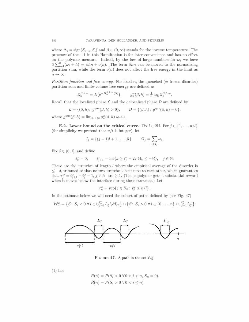
386 CARAVENNA, DEN HOLLANDER, AND PETRELIS
where ∆i = sign(Si−1, Si) and β ∈ (0,∞) stands for the inverse temperature. Thepresence of the −1 in this Hamiltonian is for later convenience and has no effecton the polymer measure. Indeed, by the law of large numbers for ω, we haveβ∑ni=1(ωi + h) = βhn + o(n). The term βhn can be moved to the normalizing
partition sum, while the term o(n) does not affect the free energy in the limit asn→ ∞.
Partition function and free energy. For fixed n, the quenched (= frozen disorder)partition sum and finite-volume free energy are defined as
Zβ,h,ωn = E(e−H
β,h,ωn (S)
), gωn (β, h) =
1n logZβ,h,ωn .
Recall that the localized phase L and the delocalized phase D are defined by
L = (β, h) : gque(β, h) > 0, D = (β, h) : gque(β, h) = 0,where gque(β, h) = limn→∞ gωn(β, h) ω-a.s.
E.2. Lower bound on the critical curve. Fix l ∈ 2N. For j ∈ 1, . . . , n/l(for simplicity we pretend that n/l is integer), let
Ij = (j − 1)l + 1, . . . , jl, Ωj =∑
i∈Ij
ωi.
Fix δ ∈ (0, 1], and define
iω0 = 0, iωj+1 = infk ≥ iωj + 2: Ωk ≤ −δl, j ∈ N.
These are the stretches of length l where the empirical average of the disorder is≤ −δ, trimmed so that no two stretches occur next to each other, which guaranteesthat τωj = iωj+1 − iωj − 1, j ∈ N, are ≥ 1. (The copolymer gets a substantial reward
when it moves below the interface during these stretches.) Let
tωn = supj ∈ N0 : iωj ≤ n/l.
In the estimate below we will need the subset of paths defined by (see Fig. 47)
Wωn =
S : Si < 0 ∀ i ∈ ∪t
ωn
j=1Iiωj \∂Iiωj∩S : Si > 0 ∀ i ∈ 0, . . . , n \ ∪t
ωn
j=1Iiωj.
n
τω1 l τω2 l
Iiω1 Iiω2 Iitωn
Figure 47. A path in the set Wωn .
(1) Let
R(n) = P (Si > 0 ∀ 0 < i < n, Sn = 0),
R(n) = P (Si > 0 ∀ 0 < i ≤ n).

LECTURES ON RANDOM POLYMERS 387
Insert the indicator of the set Wωn into the definition of the partition sum, to
estimate
logZβ,h,ωn ≥tωn∑
j=1
logR(τωj l) + tωn [logR(l) + 2β(δ − h)l] + log R(n− itωn l).
(2) Note that there exists a C > 0 such that R(n) ≥ C/n3/2 for n ∈ N. Use this todeduce from (1) that
logZβ,h,ωn ≥ tωn[logC− 3
2 log( ntωn− l)
]+ tωn
[logC − 3
2 log l+2β(δ− h)l]+O(logn),
where the first term arises after we apply Jensen’s inequality:
1
tωn
tωn∑
j=1
log τωj ≤ log
1
tωn
tωn∑
j=1
τωj
.
(3) Abbreviate
ql,δ = P
(Ω1 ≤ −δl
).
Use the ergodic theorem to prove that
limn→∞
tωnn
=1
l
ql,δ1 + ql,δ
= pl,δ ω-a.s..
(Note that k ∈ ∪j∈N0iωj if and only if Ωk ≤ −δl and k − 1 /∈ ∪j∈N0
iωj .) Since∑tωnj=1 τ
ωj l ≤ n− tωnl, it follows that
lim supn→∞
∑tωnj=1 τ
ωi l
tωn≤ lim
n→∞
n− tωnl
tωn= p−1
l,δ − l ω-a.s.
Conclude from (2) that
lim infn→∞
1
nlogZβ,h,ωn ≥ pl,δ[− 3
2 log(p−1l,δ − l) + 2β(δ − h)l +O(log l)] ω-a.s.
This inequality is valid for all l ∈ 2N.
(4) Show, with the help of Cramer’s theorem of large deviation theory applied toω, that
liml→∞
1l log ql,δ = − sup
λ>0
[λδ − logM(−λ)
]= −Σ(δ),
where M(λ) = E(eλω1), the supremum may be trivially restricted to λ > 0, andthe right-hand side is the Legendre transform of the cumulant generating functionλ 7→ logM(−λ). Use the last display and the relation p−1
l,δ − l = l/ql,δ to show that
liml→∞
1l log(p
−1l,δ − l) = Σ(δ).
(5) So far δ ∈ (0, 1] is arbitrary. Now combine (3) and (4), optimize over δ, and usethat
34 logM(43β) = sup
δ∈(0,1]
[− 3
4Σ(δ) + βδ]= 3
4 supδ∈(0,1]
[43βδ − Σ(δ)
],
which is the (inverse) Legendre transform of the rate function in Cramer’s theorem,to conclude that gque(β, h) > 0 as soon as
34 logM(43β)− βh > 0.
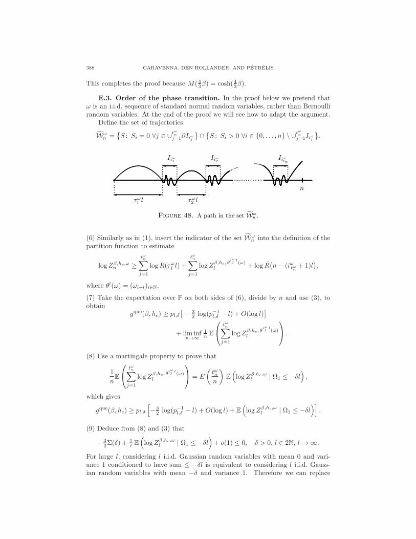
388 CARAVENNA, DEN HOLLANDER, AND PETRELIS
This completes the proof because M(43β) = cosh(43β).
E.3. Order of the phase transition. In the proof below we pretend thatω is an i.i.d. sequence of standard normal random variables, rather than Bernoullirandom variables. At the end of the proof we will see how to adapt the argument.
Define the set of trajectories
Wωn =
S : Si = 0 ∀j ∈ ∪t
ωn
j=1∂Iiωj∩S : Si > 0 ∀i ∈ 0, . . . , n \ ∪t
ωn
j=1Iiωj.
n
τω1 l τω2 l
Iiω1
Iiω2
Iiωtn
Figure 48. A path in the set Wωn .
(6) Similarly as in (1), insert the indicator of the set Wωn into the definition of the
partition function to estimate
logZβ,hc,ωn ≥tωn∑
j=1
logR(τωj l) +
tωn∑
j=1
logZβ,hc, θ
iωj l(ω)l + log R
(n− (iωtωn + 1)l
),
where θl(ω) = (ωi+l)i∈N.
(7) Take the expectation over P on both sides of (6), divide by n and use (3), toobtain
gque(β, hc) ≥ pl,δ[− 3
2 log(p−1l,δ − l) +O(log l)
]
+ lim infn→∞
1n E
tωn∑
j=1
logZβ,hc, θ
iωj l(ω)l
.
(8) Use a martingale property to prove that
1
nE
tωn∑
j=1
logZβ,hc, θ
iωj l(ω)l
= E
(tωnn
)E
(logZβ,hc,ωl | Ω1 ≤ −δl
),
which gives
gque(β, hc) ≥ pl,δ
[− 3
2 log(p−1l,δ − l) +O(log l) + E
(logZβ,hc,ωl | Ω1 ≤ −δl
)].
(9) Deduce from (8) and (3) that
− 32Σ(δ) +
1l E
(logZβ,hc,ωl | Ω1 ≤ −δl
)+ o(1) ≤ 0, δ > 0, l ∈ 2N, l → ∞.
For large l, considering l i.i.d. Gaussian random variables with mean 0 and vari-ance 1 conditioned to have sum ≤ −δl is equivalent to considering l i.i.d. Gauss-ian random variables with mean −δ and variance 1. Therefore we can replace
LECTURES ON RANDOM POLYMERS 389
E(logZβ,hc,ωl | Ω1 ≤ −δl) by E(logZβ,hc−δ,ωl ) + o(1) and so, after we let l → ∞,the inequality in the last display yields
gque(β, hc − δ) ≤ 32Σ0(δ).
Combine the lower bound on gque(β, hc) with the upper bound on gque(β, hc − δ),and use that Σ0(δ) =
12δ
2[1 + o(1)] as δ ↓ 0, to obtain that
gque(β, hc − δ)− g(β, hc) ≤ 14δ
2 for δ small enough.
This completes the proof for standard Gaussian disorder.
(10) It is easy to extend the proof to binary disorder. All that is needed is to showthat the Gaussian approximation in (9) carries through.
References
[1] K.S. Alexander, Ivy on the ceiling: first-order polymer depinning transitions with quencheddisorder, Markov Proc. Relat. Fields 13 (2007) 663–680.
[2] K.S. Alexander, The effect of disorder on polymer depinning transitions, Commun. Math.Phys. 279 (2008) 117–146.
[3] K.S. Alexander and V. Sidoravicius, Pinning of polymers and interfaces by random poten-tials, Ann. Appl. Probab. 16 (2006) 636–669.
[4] K.S. Alexander and N. Zygouras, Quenched and annealed critical points in polymer pinningmodels, Commun. Math. Phys. 291 (2008) 659–689.
[5] K.S. Alexander and N. Zygouras, Equality of critical points for polymer depinning transitionswith loop exponent one, Ann. Appl. Probab. 20 (2010) 356–66.
[6] L. Auvray, B. Duplantier, A. Echard and C. Sykes, Physique des polymeres et membranesbiologiques, Partie 1, Ecole Polytechnique, Palaiseau, France.
[7] R. Bauerschmidt, H. Duminil-Copin, J. Goodman, G. Slade, Lectures on self-avoiding walks,in this volume.
[8] V. Beffara, Schramm-Loewner evolution and other conformally invariant objects, in thisvolume.
[9] Q. Berger and F.L. Toninelli, On the critical point of the random walk pinning model indimension d = 3, Electr. J. Probab. 15 (2010) 654–683.
[10] S. Bezerra, S. Tindel and F. Viens, Superdiffusivity for a Brownian polymer in a continuousGaussian environment, Ann. Probab. 36 (2008) 1642–1675.
[11] M. Birkner, A condition for weak disorder for directed polymers in random environment,Electr. Comm. Prob. 9 (2004) 22–25.
[12] M. Birkner, A. Greven and F. den Hollander, Quenched large deviation principle for wordsin a letter sequence, Probab. Theory Relat. Fields 148 (2010) 403–456.
[13] M. Birkner, A. Greven and F. den Hollander, Collision local time of transient random walksand intermediate phases in interacting stochastic systems, Electr. J. Probab. 16 (2011) 552–586.
[14] M. Birkner and R. Sun, Annealed vs quenched critical points for a random walk pinningmodel, Ann. Inst. H. Poincare Probab. Stat. 46 (2010) 414–441.
[15] M. Birkner and R. Sun, Disorder relevance for the random walk pinning model in dimension3, Ann. Inst. H. Poincare Probab. Stat. 47 (2011) 259–293.
[16] M. Biskup and F. den Hollander, A heteropolymer near a linear interface, Ann. Appl.Probab. 9 (1999) 668–687.
[17] T. Bodineau and G. Giacomin, On the localization transition of random copolymers nearselective interfaces, J. Stat. Phys. 117 (2004) 801–818.
[18] T. Bodineau, G. Giacomin, H. Lacoin and F.L. Toninelli, Copolymers at selective interfaces:new bounds on the phase diagram, J. Stat. Phys. 132 (2008) 603–626.
[19] E. Bolthausen, A note on diffusion of directed polymers in a random environment, Commun.Math. Phys. 123 (1989) 529–534.
[20] E. Bolthausen, F. Caravenna and B. de Tiliere, The quenched critical point of a diluteddisordered polymer model, Stoch. Proc. Appl. 119 (2009) 1479–1504.
390 CARAVENNA, DEN HOLLANDER, AND PETRELIS
[21] E. Bolthausen and F. den Hollander, Localization transition for a polymer near an interface,Ann. Probab. 25 (1997) 1334–1366.
[22] E. Bolthausen, F. den Hollander and A. Opoku, A copolymer near a selective interface:variational characterization of the free energy, arXiv.org: 1110.1315 [math.PR], manuscriptin preparation.
[23] R. Brak, A.J. Guttmann and S.G. Whittington, A collapse transition in a directed walkmodel, J. Phys. A: Math. Gen. 25 (1992) 2437–2446.
[24] A. Camanes and P. Carmona, The critical temperature of a directed polymer in a randomenvironment, Markov Proc. Relat. Fields 15 (2009) 105–116.
[25] P. Caputo, F. Martinelli and F.L. Toninelli, On the approach to equilibrium for a polymerwith adsorption and repulsion, Electr. J. Probab. 13 (2008) 213–258.
[26] P. Caputo, H. Lacoin, F. Martinelli, F. Simenhaus and F.L. Toninelli, Polymer dynam-ics in the depinned phase: metastability with logarithmic barriers, arXiv.org: 1007.4470[math.PR], to appear in Probab. Theory Relat. Fields.
[27] F. Caravenna and G. Giacomin, The weak coupling limit of disordered copolymer models,Ann. Probab. 38 (2010) 2322–2378.
[28] F. Caravenna, G. Giacomin and M. Gubinelli, A numerical approach to copolymers atselective interfaces, J. Stat. Phys. 122 (2006) 799–832.
[29] F. Caravenna, G. Giacomin and F.L. Toninelli, Copolymers at selective interfaces: settled
issues and open problems, In: Probability in complex physical systems. In honour of ErwinBolthausen and Jrgen Grtner. Edited by J.-D. Deuschel, B. Gentz, W. Knig, M. von Renesse,M. Scheutzow, U. Schmock. Springer Proceedings in Mathematics 11 (2012), 289-312.
[30] F. Caravenna, G. Giacomin and L. Zambotti, Sharp asymptotic behavior for wetting modelsin (1+1)-dimension, Electr. J. Probab. 11 (2006) 345–362.
[31] F. Caravenna and N. Petrelis, A polymer in a multi-interface medium, Ann. Appl. Probab.19 (2009) 1803–1839.
[32] F. Caravenna and N. Petrelis, Depinning of a polymer in a multi-interface medium, Electr.J. Probab. 14 (2009) 2038–2067.
[33] P. Carmona and Y. Hu, On the partition function of a directed polymer in a Gaussianrandom environment, Probab. Theory Relat. Fields 124 (2002) 431–457.
[34] P. Carmona and Y. Hu, Fluctuation exponents and large deviations for directed polymersin a random environment, Stoch. Proc. Appl. 112 (2004) 285–308.
[35] D. Cheliotis and F. den Hollander, Variational characterization of the critical curve forpinning of random polymers, arXiv.org: 1005.3661v1 [math.PR], to appear in Ann. Probab.
[36] N. Clisby, R. Liang and G. Slade, Self-avoiding walk enumeration via the lace expansion. J.Phys. A: Math. Theor. 40 (2007) 10973–11017.
[37] F. Comets, T. Shiga and N. Yoshida, Directed polymers in random environment: Pathlocalization and strong disorder, Bernoulli 9 (2003) 705–723.
[38] F. Comets, T. Shiga and N. Yoshida, Probabilistic analysis of directed polymers in a randomenvironment: a review, in: Stochastic Analysis on Large Scale Systems, Adv. Stud. PureMath. 39 (2004), pp. 115–142.
[39] F. Comets and V. Vargas, Majorizing multiplicative cascades for directed polymers in ran-dom media, Alea 2 (2006) 267–277.
[40] F. Comets and N. Yoshida, Brownian directed polymers in random environment, Commun.Math. Phys. 254 (2004) 257–287.
[41] F. Comets and N. Yoshida, Some new results on Brownian directed polymers in randomenvironment, RIMS Kokyuroku 1386 (2004) 50–66.
[42] F. Comets and N. Yoshida, Directed polymers in random environment are diffusive at weakdisorder, Ann. Probab. 34 (2006) 1746–1770.
[43] L.N. Coyle, A continuous time version of random walks in a random potential, Stoch. Proc.Appl. 64 (1996) 209–235.
[44] L.N. Coyle, Infinite moments of the partition function for random walks in a random po-tential, J. Math. Phys. 39 (1998) 2019–2034.
[45] D. Cule and T. Hwa, Denaturation of heterogeneous DNA, Phys. Rev. Lett. 79 (1997)2375–2378.
[46] D.A. Dawson and J. Gartner, Large deviations from the McKean-Vlasov limit for weaklyinteracting diffusions, Stochastics 20 (1987) 247–308.
[47] A. Dembo and O. Zeitouni, Large Deviations Techniques and Applications, Springer, 1998.
LECTURES ON RANDOM POLYMERS 391
[48] B. Derrida, G. Giacomin, H. Lacoin and F.L. Toninelli, Fractional moment bounds anddisorder relevance for pinning models, Commun. Math. Phys. 287 (2009) 867–887.
[49] J.-D. Deuschel, G. Giacomin and L. Zambotti, Scaling limits of equilibrium wetting modelsin (1+1)-dimension, Probab. Theory Relat. Fields 132 (2005) 471–500.
[50] H. Duminil-Copin and S. Smirnov, Conformal invariance of lattice models, in this volume.[51] B. Duplantier and H. Saleur, Exact tricritical exponents for polymers at the FTHETA point
in two dimensions, Phys. Rev. Lett. 59 (1987) 539–542.[52] M.R. Evans and B. Derrida, Improved bounds for the transition temperature of directed
polymers in a finite-dimensional random medium, J. Stat. Phys. 69 (1992) 427–437.[53] M.E. Fisher, Walks, walls, wetting and melting, J. Stat. Phys. 34 (1984) 667–729.[54] C. Garban and J.E. Steif, Noise-sensitivity and percolation, in this volume.[55] G. Giacomin, Random Polymer Models, Imperial College Press, London, 2007.[56] G. Giacomin, H. Lacoin and F.L. Toninelli, Marginal relevance of disorder for pinning mod-
els, Commun. Pure Appl. Math. 63 (2010) 233–265.[57] G. Giacomin, H. Lacoin and F.L. Toninelli, Disorder relevance at marginality and critical
point shift, Ann. Inst. H. Poincare Probab. Stat. 47 (2011) 148–175.[58] G. Giacomin and F.L. Toninelli, Estimates on path delocalization for copolymers at selective
interfaces, Probab. Theory Relat. Fields 133 (2005) 464–482.[59] G. Giacomin and F.L. Toninelli, Smoothing of depinning transitions for directed polymers
with quenched disorder, Phys. Rev. Lett. 96 (2006) 070602.[60] G. Giacomin and F.L. Toninelli, Smoothing effect of quenched disorder on polymer depinning
transitions, Commun. Math. Phys. 266 (2006) 1–16.[61] G. Giacomin and F.L. Toninelli, The localized phase of disordered copolymers with adsorp-
tion, Alea 1 (2006) 149–180.[62] G. Giacomin and F.L. Toninelli, Force-induced depinning of directed polymers, J. Phys. A:
Math. Gen. 40 (2007) 5261–5275.[63] G. Giacomin and F.L. Toninelli, On the irrelevant disorder regime of pinning models, Ann.
Probab. 37 (2009) 1841–1875.[64] A.J. Guttmann (Ed.), Polygons, Polyominoes and Polycubes, Lecture Notes in Physics 775,
Springer and Canopus Academic Publishing Ltd., 2009.[65] T. Hara and G. Slade, Self-avoiding walk in five or more dimensions, I. The critical behaviour,
Commun. Math. Phys. 147 (1992) 101–136.[66] T. Hara and G. Slade, The lace expansion for self-avoiding walk in five or more dimensions,
Rev. Math. Phys. 4 (1992) 235–327.[67] R. van der Hofstad and A. Klenke, Self-attractive random polymers, Ann. Appl. Prob. 11
(2001) 1079–1115.[68] R. van der Hofstad, A. Klenke and W. Konig, The critical attractive random polymer in
dimension one, J. Stat. Phys. 106 (2002) 477–520.[69] F. den Hollander, Large Deviations, Fields Institute Monographs, AMS, Providence RI,
2000.[70] F. den Hollander, Random Polymers, Lecture Notes in Mathematics 1974, Springer, Berlin,
2009.[71] F. den Hollander and N. Petrelis, On the localized phase of a copolymer in an emulsion:
supercritical percolation regime, Commun. Math. Phys. 285 (2009) 825–871.[72] F. den Hollander and N. Petrelis, On the localized phase of a copolymer in an emulsion:
subcritical percolation regime, J. Stat. Phys. 134 (2009) 209–241.[73] F. den Hollander and N. Petrelis, A mathematical model for a copolymer in an emulsion, J.
Math. Chem. 48 (2010) 83–94.[74] F. den Hollander and N. Petrelis, Free energy of a copolymer in a micro-emulsion, arXiv.org:
1204.1234 [math.PR], manuscript in preparation.[75] F. den Hollander and S.G. Whittington, Localization transition for a copolymer in an emul-
sion, Theor. Prob. Appl. 51 (2006) 193–240.[76] J.Z. Imbrie and T. Spencer, Diffusion of directed polymers in a random environment, J.
Stat. Phys. 52 (1988) 609–626.[77] D. Ioffe and Y. Velenik, The statistical mechanics of stretched polymers, Braz. J. Probab.
Stat. 24 (2010) 279–299.[78] D. Ioffe and Y. Velenik, Crossing random walks and stretched polymers at weak disorder,
arXiv.org: 1002.4289v2 [math.PR], to appear in Ann. Probab.
392 CARAVENNA, DEN HOLLANDER, AND PETRELIS
[79] D. Ioffe and Y. Velenik, Stretched polymers in random environment, arXiv.org: 1011.0266v1[math.PR].
[80] D. Ioffe and Y. Velenik, Self-attractive random walks: The case of critical drifts, arXiv.org:1104.4615v1 [math.PR].
[81] I. Jensen, homepage (www.ms.unimelb.edu.au/∼iwan).[82] Y. Kafri, D. Mukamel and L. Peliti, Why is the DNA denaturation transition first order?,
Phys. Rev. Lett. 85 (2000) 4988–4991.[83] H. Lacoin, New bounds for the free energy of directed polymer in dimension 1+1 and 1+2,
Commun. Math. Phys. 294 (2010) 471–503.[84] H. Lacoin, The martingale approach to disorder relevance for pinning models, Electr. Comm.
Probab. 15 (2010) 418–427.[85] H. Lacoin, Influence of spatial correlation for directed polymers, Ann. Probab. 39 (2011)
139–175.[86] M. Ledoux, The Concentration of Measure Phenomenon, Mathematical Surveys and Mono-
graphs 89, American Mathematical Society, 2001.[87] O. Mejane, Upper bound of a volume exponent for directed polymers in a random environ-
ment, Ann. Inst. H. Poincare Probab. Stat. 40 (2004) 299–308.[88] M. Petermann, Superdiffusivity of directed polymers in random environment, Ph.D. thesis,
University of Zurich, 2000.
[89] N. Petrelis, Localisation d’un Polymere en Interaction avec une Interface, Ph.D. Thesis,University of Rouen, France, February 2, 2006.
[90] N. Petrelis, Polymer pinning at an interface, Stoch. Proc. Appl. 116 (2006) 1600–1621.[91] N. Petrelis, Copolymer at selective interfaces and pinning potentials: weak coupling limits,
Ann. Inst. H. Poincare Probab. Stat. 45 (2009) 175–200.[92] M.S.T. Piza, Directed polymers in a random environment: some results on fluctuations, J.
Stat. Phys. 89 (1997) 581–603.[93] R.D. Schram, G.T. Barkema and R.H. Bisseling, Exact enumeration of self-avoiding walks,
arXiv.org: 1104.2184 [physics.math-ph].[94] F. Seno and A.L. Stella, θ point of a linear polymer in 2 dimensions: a renormalization
group analysis of Monte Carlo enumerations, J. Physique 49 (1988) 739–748.[95] Ya.G. Sinai, A remark concerning random walks with random potentials, Fund. Math. 147
(1995) 173–180.[96] J. Sohier, Finite size scaling for homogene¡ous pinning models, ALEA 6 (2009) 163–177.[97] F. Spitzer, Principles of Random Walk (2nd. ed.), Springer, New York, 1976.[98] J.M. Steele, Kingman’s subadditive ergodic theorem, Ann. Inst. Henri Poincare 25 (1989)
93–98.[99] M.C. Tesi, E.J. Janse van Rensburg, E. Orlandini and S.G. Whittington, Monte Carlo study
of the interacting self-avoiding walk model in three dimensions, J. Stat. Phys. 82 (1996) 155–181.
[100] F.L. Toninelli, A replica-coupling approach to disordered pinning models, Commun. Math.Phys. 280 (2008) 389–401.
[101] F.L. Toninelli, Disordered pinning models and copolymers: beyond annealed bounds, Ann.Appl. Probab. 18 (2008) 1569–1587.
[102] F.L. Toninelli, Coarse graining, fractional moments and the critical slope of random poly-mers, Electr. J. Probab. 14 (2009) 531–547.
[103] F.L. Toninelli, Localization transition in disordered pinning models. Effect of randomnesson the critical properties, in: Lecture Notes in Mathematics 1970, Springer, Berlin, 2009,pp. 129-176.
[104] N. Zygouras, Lyapounov norms for random walks in low disorder and dimension greaterthan three, Probab. Theory Relat. Fields 143 (2009) 667–683.
[105] N. Zygouras, Strong disorder in semidirected random polymers, arXiv.org: 1009.2693v2[math.PR].
LECTURES ON RANDOM POLYMERS 393
Dipartimento di Matematica e Applicazioni, Universita degli Studi di Milano - Bic-
occa, Via Cozzi 53, 20125 Milano, Italy
E-mail address: [email protected]
Mathematical Institute, Leiden University, P.O. Box 9512, 2300 RA Leiden, The
Netherlands
E-mail address: [email protected]
Laboratoire de Mathematiques Jean Leray, 2 rue de la Houssiniere - BP 92208,
F-44322 Nantes Cedex 3, France
E-mail address: [email protected]


![Lecture on Intrinsically conducting polymers on textiles [EN] · Conducting polymers • Intrinsically conducting polymers (ICPs) are π-conjugated organic polymers able to conduct](https://img.pdfslide.us/doc/110x75/5f07a9317e708231d41e19a9/lecture-on-intrinsically-conducting-polymers-on-textiles-en-conducting-polymers.jpg)


![Laurence W. McKeen, PhD - Pentasil Used in Medical Devices.pdf · of branched polymers include star polymers, comb polymers, brush polymers, dendronized polymers [1], ladders, and](https://img.pdfslide.us/doc/110x75/5fd30108783da00f76371237/laurence-w-mckeen-phd-pentasil-used-in-medical-devicespdf-of-branched-polymers.jpg)