Embed Size (px)
Citation preview
Lectures on random lozenge tilings
Vadim Gorin
University of Wisconsin–Madison,Massachusetts Institute of Technology,
andInstitute for Information Transmission Problems of Russian Academy
of Sciences.
This material will be published by Cambridge University Press as“Lectures on Random Lozenge Tilings” by Vadim Gorin. This
prepublication version is free to view and download for personal useonly. Not for redistribution, resale or use in derivative works.

Contents
About this book page 6
1 Lecture 1: Introduction and tileability. 71.1 Preface 71.2 Motivation 91.3 Mathematical questions 101.4 Thurston’s theorem on tileability 151.5 Other classes of tilings and reviews. 20
2 Lecture 2: Counting tilings through determinants. 212.1 Approach 1: Kasteleyn formula 212.2 Approach 2: Lindstrom-Gessel-Viennot lemma 252.3 Other exact enumeration results 30
3 Lecture 3: Extensions of the Kasteleyn theorem. 313.1 Weighted counting 313.2 Tileable holes and correlation functions 333.3 Tilings on a torus 34
4 Lecture 4: Counting tilings on large torus. 394.1 Free energy 394.2 Densities of three types of lozenges 414.3 Asymptotics of correlation functions 44
5 Lecture 5: Monotonicity and concentration for tilings 465.1 Monotonicity 465.2 Concentration 485.3 Limit shape 50
6 Lecture 6: Slope and free energy. 526.1 Slope in a random weighted tiling 526.2 Number of tilings of a fixed slope 546.3 Concentration of the slope 566.4 Limit shape of a torus 57
3
4 Contents
7 Lecture 7: Maximizers in the variational principle 587.1 Review 587.2 The definition of surface tension and class of functions 597.3 Upper semicontinuity 627.4 Existence of the maximizer 647.5 Uniqueness of the maximizer 65
8 Lecture 8: Proof of the variational principle. 67
9 Lecture 9: Euler-Lagrange and Burgers equations. 749.1 Euler-Lagrange equations 749.2 Complex Burgers equation via a change of coordinates 759.3 Generalization to qVolume–weighted tilings 789.4 Complex characteristics method 79
10 Lecture 10: Explicit formulas for limit shapes 8110.1 Analytic solutions to the Burgers equation 8110.2 Algebraic solutions 8410.3 Limit shapes via quantized Free Probability 86
11 Lecture 11: Global Gaussian fluctuations for the heights. 9011.1 Kenyon-Okounkov conjecture 9011.2 Gaussian Free Field 9211.3 Gaussian Free Field in Complex Structures 96
12 Lecture 12: Heuristics for the Kenyon-Okounkov conjecture 98
13 Lecture 13: Ergodic translation-invariant Gibbs measures 10513.1 Tilings of the plane 10513.2 Properties of the local limits 10713.3 Slope of EGTI measure 10913.4 Correlation functions of EGTI measures 11113.5 Frozen, liquid, and gas phases 112
14 Lecture 14: Inverse Kasteleyn matrix for trapezoids. 116
15 Lecture 15: Steepest descent method for asymptotic analysis. 12315.1 Setting for steepest descent 12315.2 Warm up example: real integral 12315.3 One-dimensional contour integrals 12415.4 Steepest descent for a double contour integral 126
16 Lecture 16: Bulk local limits for tilings of hexagons 129
17 Lecture 17: Bulk local limits near straight boundaries 138
5
18 Lecture 18: Edge limits of tilings of hexagons 14518.1 Heuristic derivation of two scaling exponents 14518.2 Edge limit of random tilings of hexagons 14718.3 Airy line ensemble in tilings and beyond 152
19 Lecture 19: Airy line ensemble, GUE-corners, and others 15419.1 Invariant description of the Airy line ensemble 15419.2 Local limits at special points of the frozen boundary 15619.3 From tilings to random matrices 157
20 Lecture 20: GUE–corners process and its discrete analogues. 16420.1 Density of GUE–corners process 16420.2 GUE–corners process as a universal limit 16820.3 A link to asymptotic representation theory and analysis 171
21 Lecture 21: Discrete log-gases. 17621.1 Log-gases and loop equations 17621.2 Law of Large Numbers through loop equations 17921.3 Gaussian fluctuations through loop equations 18221.4 Orthogonal polynomial ensembles 185
22 Lecture 22: Plane partitions and Schur functions. 18822.1 Plane partitions 18822.2 Schur Functions 19022.3 Expectations of observables 192
23 Lecture 23: Limit shape and fluctuations for plane partitions. 19923.1 Law of Large Numbers 19923.2 Central Limit Theorem 205
24 Lecture 24: Discrete Gaussian component in fluctuations. 20924.1 Random heights of holes 20924.2 Discrete fluctuations of heights through GFF heuristics. 21024.3 Approach through log-gases 21424.4 2d Dirichlet energy and 1d logarithmic energy. 21724.5 Discrete component in tilings on Riemann surfaces 224
25 Lecture 25: Sampling random tilings. 22525.1 Markov Chain Monte-Carlo 22525.2 Coupling from the past [ProppWilson96] 22925.3 Sampling through counting 23325.4 Sampling through bijections 23325.5 Sampling through transformations of domains 234References 236Index 248
About this book
These are lecture notes for a one semester class devoted to the study of randomtilings. It was 18.177 taught at Massachusetts Institute of Technology duringSpring of 2019. The brilliant students who participated in the class1: AndrewAhn, Ganesh Ajjanagadde, Livingston Albritten, Morris (Jie Jun) Ang, AaronBerger, Evan Chen, Cesar Cuenca, Yuzhou Gu, Kaarel Haenni, Sergei Ko-rotkikh, Roger Van Peski, Mehtaab Sawhney, Mihir Singhal provided tremen-dous help in typing the notes.
Additional material was added to most of the lectures after the class wasover. Hence, when using this review as a textbook for a class, one should notexpect to cover all the material in one semester, something should be left out.
I also would like to thank Amol Aggarwal, Alexei Borodin, Christian Krat-tenthaler, Igor Pak, Jiaming Xu, Marianna Russkikh, and Semen Shlosman fortheir useful comments and suggestions. I am grateful to Christophe Charlier,Maurice Duits, Sevak Mkrtchyan, and Leonid Petrov for the help with simula-tions of random tilings.
Funding acknowledgements. The work of V.G. was partially supportedby NSF Grants DMS-1664619, DMS-1949820, by NEC Corporation Fundfor Research in Computers and Communications, and by the Office of theVice Chancellor for Research and Graduate Education at the University ofWisconsin–Madison with funding from the Wisconsin Alumni Research Foun-dation. Chapters 6 and 13 of this work were supported by Russian ScienceFoundation (project 20-41-09009).
1 Last name alphabetic order.
6
Lecture 1: Introduction and tileability.
1.1 Preface
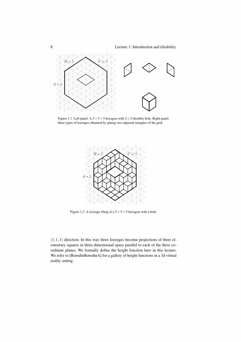
The goal of the lectures is to understand the mathematics of tilings. The generalsetup is to take a lattice domain and tile it with elementary blocks. For the mostpart, we study the special case of tiling a polygonal domain on the triangulargrid (of mesh size 1) by three kinds of rhombi that we call “lozenges”.
The left panel of Figure 1.1 shows an example of a polygonal domain onthe triangular grid. The right panel of Figure 1.1 shows the lozenges: each ofthem is obtained by gluing two adjacent lattice triangles. A triangle of the gridis surrounded by three other triangles, attaching one of them we get one ofthe three types of lozenges. The lozenges can be also viewed as orthogonalprojections onto the x+y+z = 0 plane of three sides of a unit cube. Figure 1.2provides an example of a lozenge tiling of the domain of Figure 1.1.
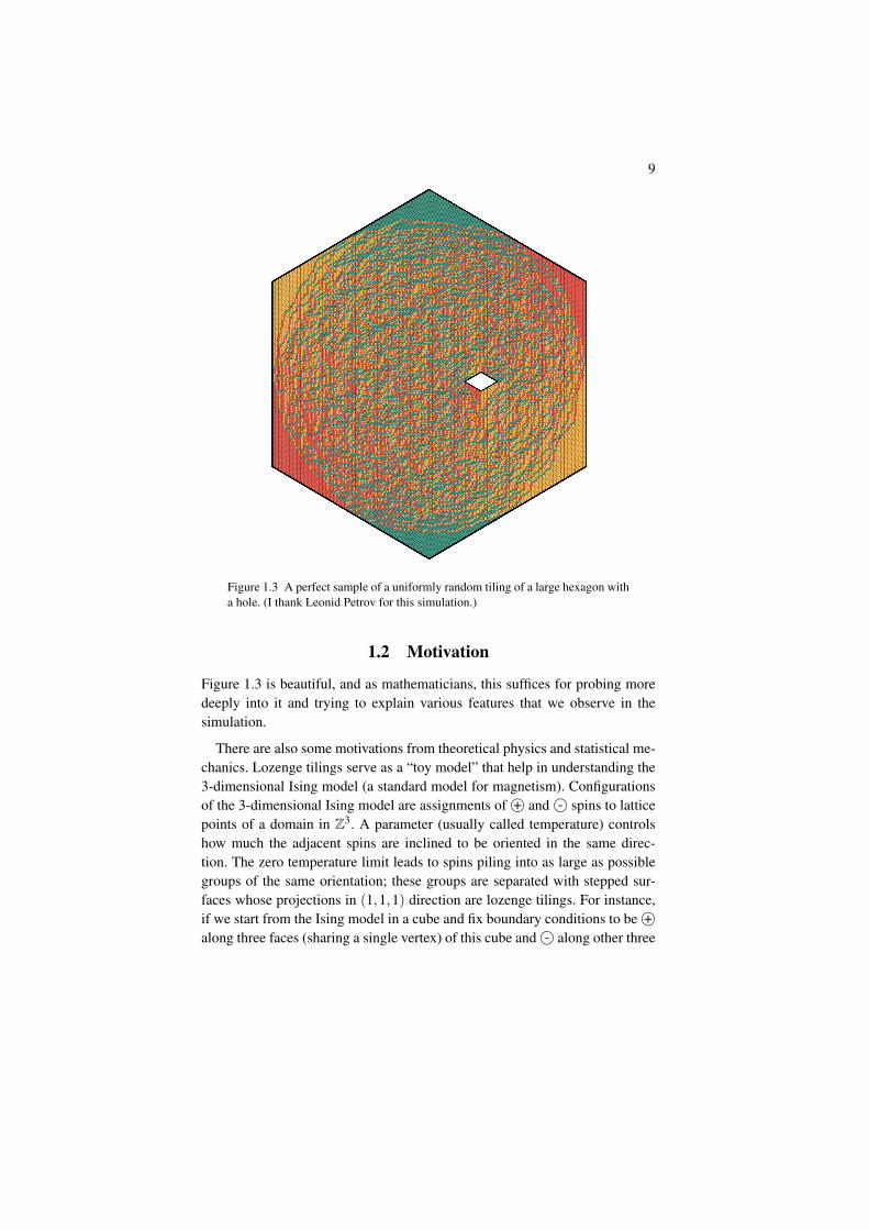
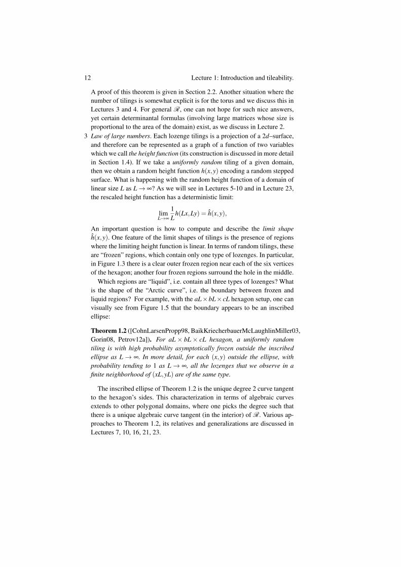
Figure 1.3 shows a lozenge tiling of a large domain, with the three types oflozenges shown in three different colors. The tiling here is generated uniformlyat random over the space of all possible tilings of this domain. More precisely,it is generated by a computer that is assumed to have access to perfectly ran-dom bits. It is certainly not clear at this stage how such “perfect sampling”may be done computationally, in fact we address this issue in the very lastlecture. Figure 1.3 is meant to capture a “typical tiling”, making sense of whatthis means is another topic that will be covered in this book. The simulation re-veals interesting features: one clearly sees next to the boundaries of the domainformation of the regions, where only one type of lozenges is observed. Theseregions are typically referred to as “frozen regions” and their boundaries are“artic curves”; their discovery and study has been one of the important drivingforces for investigations of the properties of random tilings.
We often identify a tiling with a so-called “height function”. The idea isto think of a 2-dimensional stepped surface living in 3-dimensional space andtreat tiling as a projection of such surface onto x+ y+ z = 0 plane along the
7
8 Lecture 1: Introduction and tileability.
A = 5
B = 5 C = 5
Figure 1.1 Left panel: A 5×5×5 hexagon with 2×2 rhombic hole. Right panel:three types of lozenges obtained by gluing two adjacent triangles of the grid.
A = 5
B = 5 C = 5
Figure 1.2 A lozenge tiling of a 5×5×5 hexagon with a hole.
(1,1,1) direction. In this way three lozenges become projections of three el-ementary squares in three-dimensional space parallel to each of the three co-ordinate planes. We formally define the height function later in this lecture.We refer to [BorodinBorodinA] for a gallery of height functions in a 3d virtualreality setting.
9
Figure 1.3 A perfect sample of a uniformly random tiling of a large hexagon witha hole. (I thank Leonid Petrov for this simulation.)
1.2 Motivation
Figure 1.3 is beautiful, and as mathematicians, this suffices for probing moredeeply into it and trying to explain various features that we observe in thesimulation.
There are also some motivations from theoretical physics and statistical me-chanics. Lozenge tilings serve as a “toy model” that help in understanding the3-dimensional Ising model (a standard model for magnetism). Configurationsof the 3-dimensional Ising model are assignments of +© and -© spins to latticepoints of a domain in Z3. A parameter (usually called temperature) controlshow much the adjacent spins are inclined to be oriented in the same direc-tion. The zero temperature limit leads to spins piling into as large as possiblegroups of the same orientation; these groups are separated with stepped sur-faces whose projections in (1,1,1) direction are lozenge tilings. For instance,if we start from the Ising model in a cube and fix boundary conditions to be +©along three faces (sharing a single vertex) of this cube and -© along other three
10 Lecture 1: Introduction and tileability.
faces, then we end up with lozenge tilings of a hexagon in zero temperaturelimit.1
Another deformation of lozenge tilings is the 6-vertex or square ice model,whose state space consists of configurations of the molecules H2O on the grid.There are six weights in this model (corresponding to six ways to match anoxygen with two out of the neighboring four hydrogens), and for particularchoices of the weights one discovers weighted bijections with tilings.
We refer to [Baxter82] for some information about the Ising and the six-vertex model, further motivations to study them and approaches to the analysis.In general, both Ising and six-vertex model are more complicated objects thanlozenge tilings, and they are much less understood. From this point of view,theory of random tilings that we develop in these lectures can be treated as thefirst step towards the understanding of more complicated models of statisticalmechanics.
For yet another motivation we notice that the two dimensional steppedsurfaces of our study have flat faces (these are frozen regions consisting oflozenges of one type, cf. Figures 1.3, 1.5), and, thus, are relevant for modellingfacets of crystals. One example from the everyday life here is a corner of alarge box of salt. For a particular (non-uniform) random tiling model, leadingto the shapes reminiscent of such a corner we refer to Figure 10.1 in Lecture10.
1.3 Mathematical questions
We now turn to describing the basic questions that drive the mathematical studyof tilings.
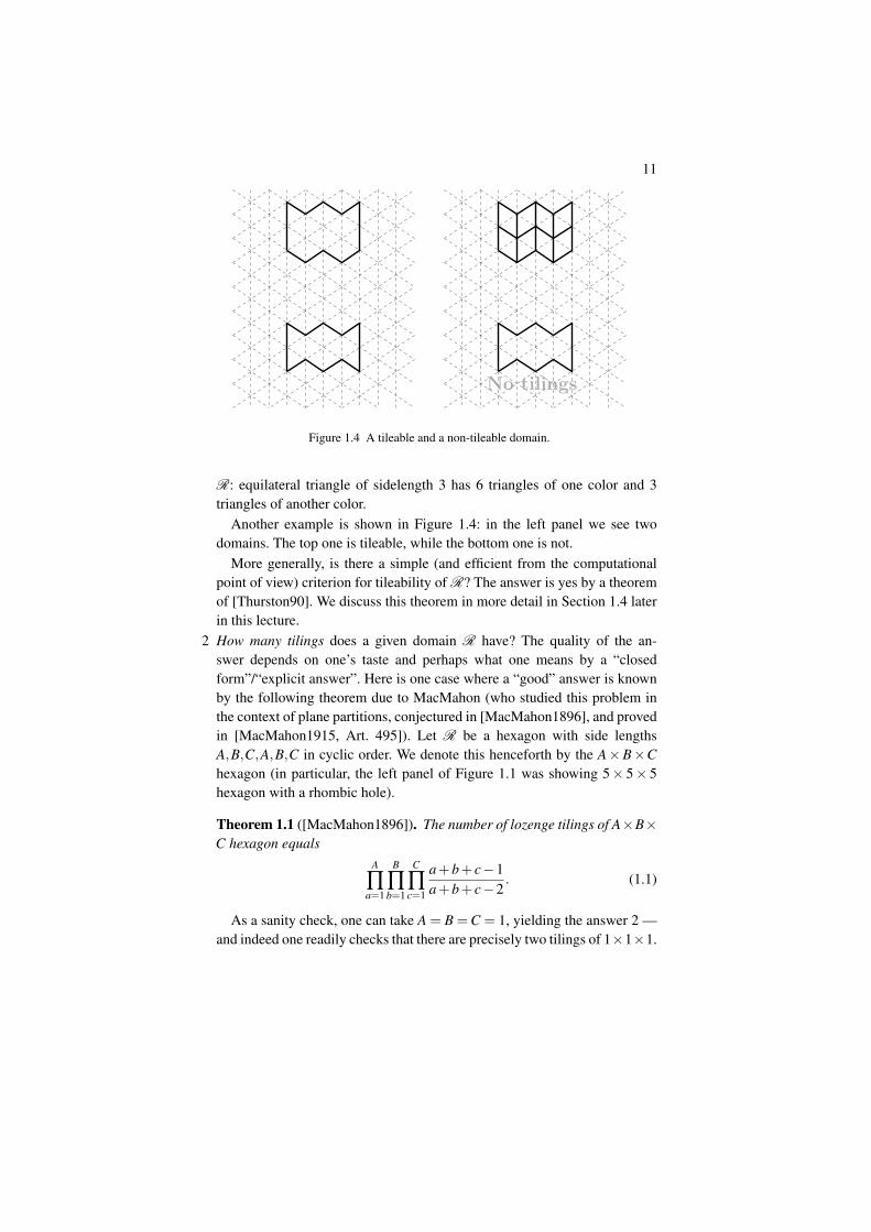
1 Existence of tilings: Given a domain R drawn on the triangular grid (andthus consisting of a finite family of triangles), does there exist a tiling of it?For example, a unit sided hexagon is trivially tileable in 2 different waysand bottom-right panel in Figure 1.2 shows one of these tilings. On theother hand, if we take the equilateral triangle of sidelength 3 as our domainR, then it is not tileable. This can be seen directly, as the corner lozengesare fixed and immediately cause obstruction. Another way to prove non-tileability is by coloring unit triangles inside R in white and black colorsin an alternating fashion. Each lozenge covers one black and one white tri-angle, but there are an unequal number of black and white triangles in the
1 See [Shlosman00, CerfKenyon01, BodineauSchonmannShlosman04] for the discussion of thecommon features between low-temperature and zero-temperature 3d Ising model, as well asthe interplay between the topics of this book and more classical statistical mechanics.
11
No tilings
Figure 1.4 A tileable and a non-tileable domain.
R: equilateral triangle of sidelength 3 has 6 triangles of one color and 3triangles of another color.
Another example is shown in Figure 1.4: in the left panel we see twodomains. The top one is tileable, while the bottom one is not.
More generally, is there a simple (and efficient from the computationalpoint of view) criterion for tileability of R? The answer is yes by a theoremof [Thurston90]. We discuss this theorem in more detail in Section 1.4 laterin this lecture.
2 How many tilings does a given domain R have? The quality of the an-swer depends on one’s taste and perhaps what one means by a “closedform”/“explicit answer”. Here is one case where a “good” answer is knownby the following theorem due to MacMahon (who studied this problem inthe context of plane partitions, conjectured in [MacMahon1896], and provedin [MacMahon1915, Art. 495]). Let R be a hexagon with side lengthsA,B,C,A,B,C in cyclic order. We denote this henceforth by the A×B×Chexagon (in particular, the left panel of Figure 1.1 was showing 5× 5× 5hexagon with a rhombic hole).
Theorem 1.1 ([MacMahon1896]). The number of lozenge tilings of A×B×C hexagon equals
A
∏a=1
B
∏b=1
C
∏c=1
a+b+ c−1a+b+ c−2
. (1.1)
As a sanity check, one can take A = B =C = 1, yielding the answer 2 —and indeed one readily checks that there are precisely two tilings of 1×1×1.
12 Lecture 1: Introduction and tileability.
A proof of this theorem is given in Section 2.2. Another situation where thenumber of tilings is somewhat explicit is for the torus and we discuss this inLectures 3 and 4. For general R, one can not hope for such nice answers,yet certain determinantal formulas (involving large matrices whose size isproportional to the area of the domain) exist, as we discuss in Lecture 2.
3 Law of large numbers. Each lozenge tilings is a projection of a 2d–surface,and therefore can be represented as a graph of a function of two variableswhich we call the height function (its construction is discussed in more detailin Section 1.4). If we take a uniformly random tiling of a given domain,then we obtain a random height function h(x,y) encoding a random steppedsurface. What is happening with the random height function of a domain oflinear size L as L→ ∞? As we will see in Lectures 5-10 and in Lecture 23,the rescaled height function has a deterministic limit:
limL→∞
1L
h(Lx,Ly) = h(x,y),
An important question is how to compute and describe the limit shapeh(x,y). One feature of the limit shapes of tilings is the presence of regionswhere the limiting height function is linear. In terms of random tilings, theseare “frozen” regions, which contain only one type of lozenges. In particular,in Figure 1.3 there is a clear outer frozen region near each of the six verticesof the hexagon; another four frozen regions surround the hole in the middle.
Which regions are “liquid”, i.e. contain all three types of lozenges? Whatis the shape of the “Arctic curve”, i.e. the boundary between frozen andliquid regions? For example, with the aL×bL× cL hexagon setup, one canvisually see from Figure 1.5 that the boundary appears to be an inscribedellipse:
Theorem 1.2 ([CohnLarsenPropp98, BaikKriecherbauerMcLaughlinMiller03,Gorin08, Petrov12a]). For aL× bL× cL hexagon, a uniformly randomtiling is with high probability asymptotically frozen outside the inscribedellipse as L→ ∞. In more detail, for each (x,y) outside the ellipse, withprobability tending to 1 as L→ ∞, all the lozenges that we observe in afinite neighborhood of (xL,yL) are of the same type.
The inscribed ellipse of Theorem 1.2 is the unique degree 2 curve tangentto the hexagon’s sides. This characterization in terms of algebraic curvesextends to other polygonal domains, where one picks the degree such thatthere is a unique algebraic curve tangent (in the interior) of R. Various ap-proaches to Theorem 1.2, its relatives and generalizations are discussed inLectures 7, 10, 16, 21, 23.
13
Figure 1.5 Arctic circle of a lozenge tiling
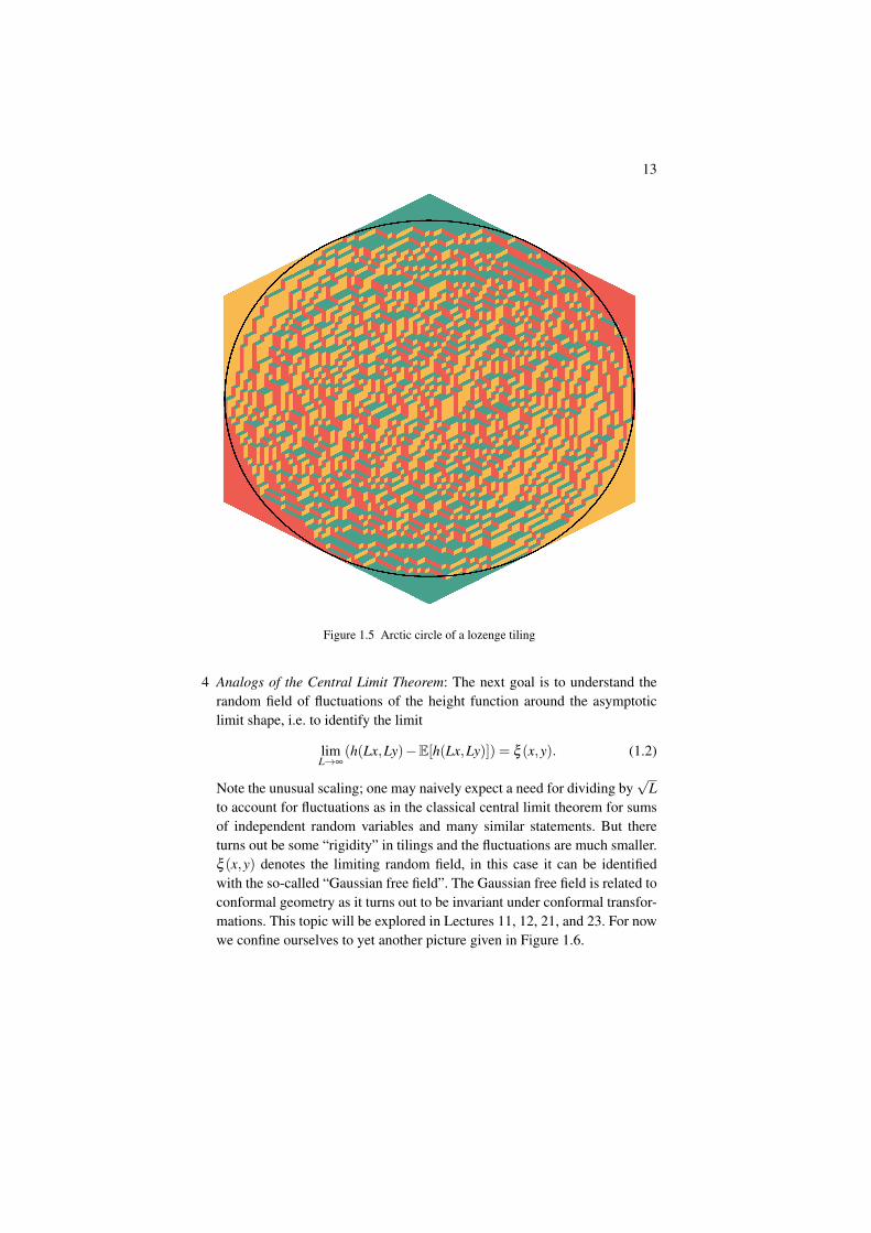
4 Analogs of the Central Limit Theorem: The next goal is to understand therandom field of fluctuations of the height function around the asymptoticlimit shape, i.e. to identify the limit
limL→∞
(h(Lx,Ly)−E[h(Lx,Ly)]) = ξ (x,y). (1.2)
Note the unusual scaling; one may naively expect a need for dividing by√
Lto account for fluctuations as in the classical central limit theorem for sumsof independent random variables and many similar statements. But thereturns out be some “rigidity” in tilings and the fluctuations are much smaller.ξ (x,y) denotes the limiting random field, in this case it can be identifiedwith the so-called “Gaussian free field”. The Gaussian free field is related toconformal geometry as it turns out to be invariant under conformal transfor-mations. This topic will be explored in Lectures 11, 12, 21, and 23. For nowwe confine ourselves to yet another picture given in Figure 1.6.
14 Lecture 1: Introduction and tileability.
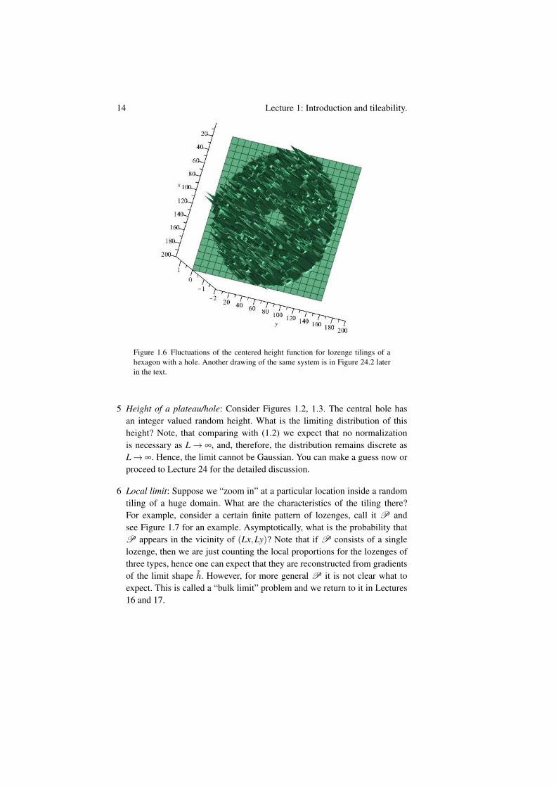
Figure 1.6 Fluctuations of the centered height function for lozenge tilings of ahexagon with a hole. Another drawing of the same system is in Figure 24.2 laterin the text.
5 Height of a plateau/hole: Consider Figures 1.2, 1.3. The central hole hasan integer valued random height. What is the limiting distribution of thisheight? Note, that comparing with (1.2) we expect that no normalizationis necessary as L→ ∞, and, therefore, the distribution remains discrete asL→ ∞. Hence, the limit cannot be Gaussian. You can make a guess now orproceed to Lecture 24 for the detailed discussion.
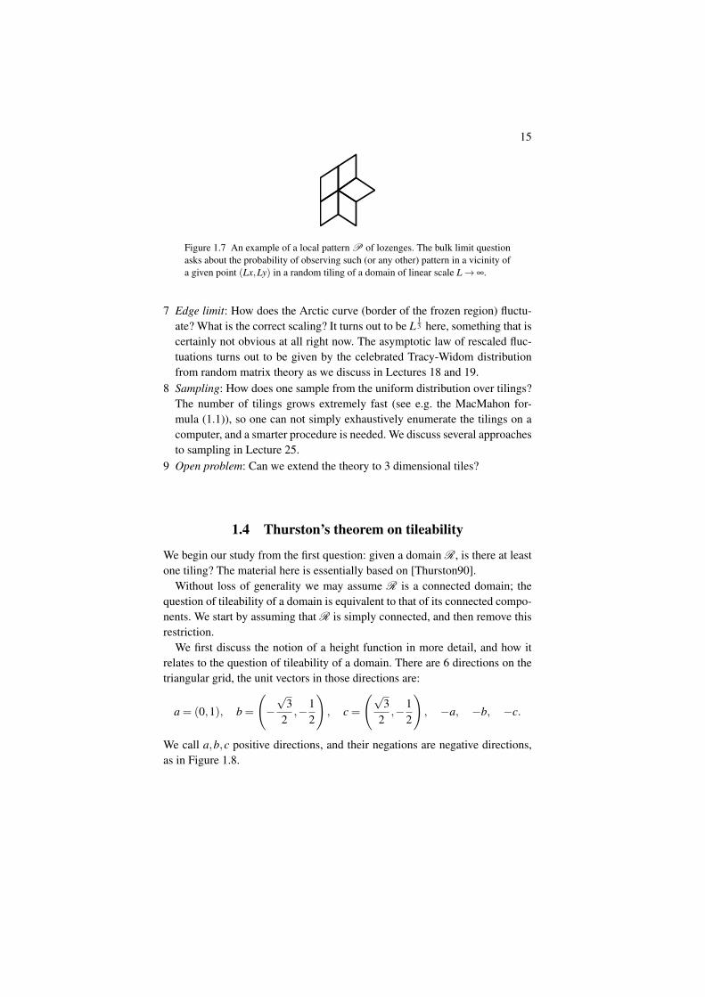
6 Local limit: Suppose we “zoom in” at a particular location inside a randomtiling of a huge domain. What are the characteristics of the tiling there?For example, consider a certain finite pattern of lozenges, call it P andsee Figure 1.7 for an example. Asymptotically, what is the probability thatP appears in the vicinity of (Lx,Ly)? Note that if P consists of a singlelozenge, then we are just counting the local proportions for the lozenges ofthree types, hence one can expect that they are reconstructed from gradientsof the limit shape h. However, for more general P it is not clear what toexpect. This is called a “bulk limit” problem and we return to it in Lectures16 and 17.
15
Figure 1.7 An example of a local pattern P of lozenges. The bulk limit questionasks about the probability of observing such (or any other) pattern in a vicinity ofa given point (Lx,Ly) in a random tiling of a domain of linear scale L→ ∞.
7 Edge limit: How does the Arctic curve (border of the frozen region) fluctu-ate? What is the correct scaling? It turns out to be L
13 here, something that is
certainly not obvious at all right now. The asymptotic law of rescaled fluc-tuations turns out to be given by the celebrated Tracy-Widom distributionfrom random matrix theory as we discuss in Lectures 18 and 19.
8 Sampling: How does one sample from the uniform distribution over tilings?The number of tilings grows extremely fast (see e.g. the MacMahon for-mula (1.1)), so one can not simply exhaustively enumerate the tilings on acomputer, and a smarter procedure is needed. We discuss several approachesto sampling in Lecture 25.
9 Open problem: Can we extend the theory to 3 dimensional tiles?
1.4 Thurston’s theorem on tileability
We begin our study from the first question: given a domain R, is there at leastone tiling? The material here is essentially based on [Thurston90].
Without loss of generality we may assume R is a connected domain; thequestion of tileability of a domain is equivalent to that of its connected compo-nents. We start by assuming that R is simply connected, and then remove thisrestriction.
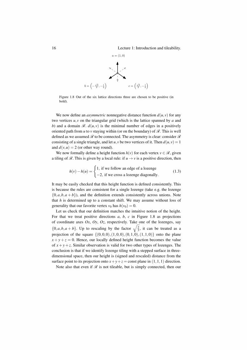
We first discuss the notion of a height function in more detail, and how itrelates to the question of tileability of a domain. There are 6 directions on thetriangular grid, the unit vectors in those directions are:
a = (0,1), b =
(−√
32
,−12
), c =
(√3
2,−1
2
), −a, −b, −c.
We call a,b,c positive directions, and their negations are negative directions,as in Figure 1.8.
16 Lecture 1: Introduction and tileability.
a = (1, 0)
b =(−
√3
2,− 1
2
)c =
(√3
2,− 1
2
)Figure 1.8 Out of the six lattice directions three are chosen to be positive (inbold).
We now define an asymmetric nonnegative distance function d(u,v) for anytwo vertices u,v on the triangular grid (which is the lattice spanned by a andb) and a domain R. d(u,v) is the minimal number of edges in a positivelyoriented path from u to v staying within (or on the boundary) of R. This is welldefined as we assumed R to be connected. The asymmetry is clear: consider R
consisting of a single triangle, and let u,v be two vertices of it. Then d(u,v) = 1and d(v,u) = 2 (or other way round).
We now formally define a height function h(v) for each vertex v ∈R, givena tiling of R. This is given by a local rule: if u→ v is a positive direction, then
h(v)−h(u) =
1, if we follow an edge of a lozenge
−2, if we cross a lozenge diagonally.(1.3)
It may be easily checked that this height function is defined consistently. Thisis because the rules are consistent for a single lozenge (take e.g. the lozenge0,a,b,a + b), and the definition extends consistently across unions. Notethat h is determined up to a constant shift. We may assume without loss ofgenerality that our favorite vertex v0 has h(v0) = 0.
Let us check that our definition matches the intuitive notion of the height.For that we treat positive directions a, b, c in Figure 1.8 as projectionsof coordinate axes Ox, Oy, Oz, respectively. Take one of the lozenges, say
0,a,b,a + b. Up to rescaling by the factor√
23 , it can be treated as a
projection of the square (0,0,0),(1,0,0),(0,1,0),(1,1,0) onto the planex+ y+ z = 0. Hence, our locally defined height function becomes the valueof x+ y+ z. Similar observation is valid for two other types of lozenges. Theconclusion is that if we identify lozenge tiling with a stepped surface in three-dimensional space, then our height is (signed and rescaled) distance from thesurface point to its projection onto x+y+ z = const plane in (1,1,1) direction.
Note also that even if R is not tileable, but is simply connected, then our
17
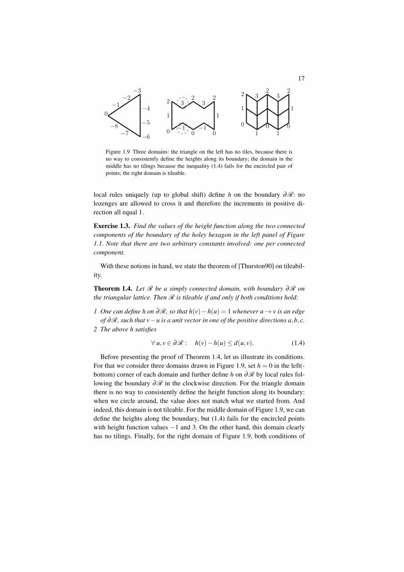
0
−1−2
−3
−4
−5
−6−7
−80
1
2 32
32
1
0 0−1 −1
0
1
2 32
32
1
0 01 1
Figure 1.9 Three domains: the triangle on the left has no tiles, because there isno way to consistently define the heights along its boundary; the domain in themiddle has no tilings because the inequality (1.4) fails for the encircled pair ofpoints; the right domain is tileable.
local rules uniquely (up to global shift) define h on the boundary ∂R: nolozenges are allowed to cross it and therefore the increments in positive di-rection all equal 1.
Exercise 1.3. Find the values of the height function along the two connectedcomponents of the boundary of the holey hexagon in the left panel of Figure1.1. Note that there are two arbitrary constants involved: one per connectedcomponent.
With these notions in hand, we state the theorem of [Thurston90] on tileabil-ity.
Theorem 1.4. Let R be a simply connected domain, with boundary ∂R onthe triangular lattice. Then R is tileable if and only if both conditions hold:
1 One can define h on ∂R, so that h(v)−h(u) = 1 whenever u→ v is an edgeof ∂R, such that v−u is a unit vector in one of the positive directions a,b,c.
2 The above h satisfies
∀ u,v ∈ ∂R : h(v)−h(u)≤ d(u,v). (1.4)
Before presenting the proof of Theorem 1.4, let us illustrate its conditions.For that we consider three domains drawn in Figure 1.9, set h = 0 in the left(-bottom) corner of each domain and further define h on ∂R by local rules fol-lowing the boundary ∂R in the clockwise direction. For the triangle domainthere is no way to consistently define the height function along its boundary:when we circle around, the value does not match what we started from. Andindeed, this domain is not tileable. For the middle domain of Figure 1.9, we candefine the heights along the boundary, but (1.4) fails for the encircled pointswith height function values −1 and 3. On the other hand, this domain clearlyhas no tilings. Finally, for the right domain of Figure 1.9, both conditions of
18 Lecture 1: Introduction and tileability.
Theorem 1.4 are satisfied; a (unique in this case) possible lozenge tiling isshown in the picture.
Proof of Theorem 1.4 Suppose R is tileable and fix any tiling. Then it definesh on all of R including ∂R by local rules (1.3). Take any positively orientedpath from u to v. Then the increments of d along this path are always 1, whilethe increments of h are either 1 or −2. Thus (1.4) holds.
Now suppose that h satisfies (1.4). Define for v ∈R:
h(v) = minu∈∂R
[d(u,v)+h(u)] . (1.5)
We call this the maximal height function extending h∣∣∂R
and corresponding tothe maximal tiling. As d is nonnegative, the definition (1.5) of h matches on∂R with the given in the theorem h
∣∣∂R
. On the other hand, since the inequalityh(v)−h(u)≤ d(u,v) necessarily holds for any height function h and any u,v∈R (by the same argument as for the case u,v ∈ ∂R above), no height functionextending h
∣∣∂R
can have larger value at v than (1.5).
Claim. h defined by (1.5) changes by 1 or −2 along each positive edge.
The claim would allow us to reconstruct the tiling uniquely: each −2 edgegives a diagonal of a lozenge and hence a unique lozenge; each triangle hasexactly one −2 edge, as the only way to position increments +1, −2 alongthree positive edges is +1+1−2 = 0; hence, we for each triangle we uniquelyreconstruct the lozenge to which it belongs. As such, we have reduced our taskto establishing the claim.
Let v→w be a positively oriented edge in R \∂R. We begin by establishingsome estimates. For any u ∈ ∂R, d(u,w)≤ d(u,v)+1 by augmenting the u,vpath by a single edge. Thus we have:
h(w)≤ h(v)+1.
Similarly, we may augment the u,w path by two positively oriented edges(at least one of the left/right pair across v,w is available) to establishd(u,v)≤ d(u,w)+2, and so:
h(w)≥ h(v)−2.
It remains to rule out 0,−1. For this, notice that any closed path on the tri-angular grid has length divisible by 3. Thus if the same boundary vertexu ∈ ∂R is involved in a minimizing path to v,w simultaneously, we see that0,−1 are ruled out by h(w) ≡ h(v) + 1 (mod 3) since any other path to whas equivalent length modulo 3 to one of the “small augmentations” above.Now suppose a different u′ is involved in a minimizing path to w, while
19
u is involved with a minimizing path to v. By looking at the closed loopu, p1(u,v), p2(v,u′), p∂ (u′,u) where p1 is a minimizing path from u to v, p2 isthe reversal of a minimizing path from w to u′ augmented similar to the above,p∂ is a segment of the boundary ∂R, we see that once again we are equiva-lent to one of the “small augmentations”. Thus, in any case h(w) = h(v)+1 orh(w) = h(v)−2 and we have completed the proof of the theorem.
How can we generalize this when R is not simply connected? We note twokey issues above:
1 It is not clear how to define h on ∂R if one is not already given a tiling. Oneach closed loop piece of ∂R we see that h is determined up to a constantshift, but these constants may differ across loops.
2 The step of the above proof that shifts from u to u′ used the fact that we couldsimply move along ∂R. This is not in general true for a multiply connecteddomain.
These issues can be addressed by ensuring that d(u,v)−h(v)+h(u) = 3k(u,v)for k(u,v) ∈ N, ∀u,v, and simply leaving the ambiguity in h as it is:
Corollary 1.5. Let R be a non-simply connected domain, with boundary ∂R
on the triangular lattice. Define h along ∂R; this is uniquely defined up toconstants c1,c2, . . . ,cl corresponding to constant shifts along the l pieces of∂R. Then R is tileable if and only if there exist c1, . . . ,cl such that for every uand v in ∂R:
d(u,v)−h(v)+h(u)≥ 0, (1.6a)
d(u,v)−h(v)+h(u)≡ 0 (mod 3). (1.6b)
Proof of Corollary 1.5 ⇒: (1.6a) ensures that this part of the proof of The-orem 1.4 remains valid; (1.6b) is also true when we have a tiling, again bythe above proof. ⇐: The shift from u to u′ is now valid, so the proof carriesthrough.
We remark that Thurston’s theorem 1.4 and the associated height func-tion method provide a O(|R| log(|R|)) time algorithm for tileability. Thereare recent improvements, see e.g. [PakShefferTassy16, Thm. 1.2] for anO(|∂R| log(|∂R|)) algorithm in the simply-connected case. [Thiant03] pro-vides an O(|R|l + a(R)) algorithm, where l denotes the number of holesin R, and a(R) denotes the area of all the holes of R. We also refer to[PakShefferTassy16, Section 5] for the further discussion of the optimal al-gorithms for tileability from the computer science literature.
20 Lecture 1: Introduction and tileability.
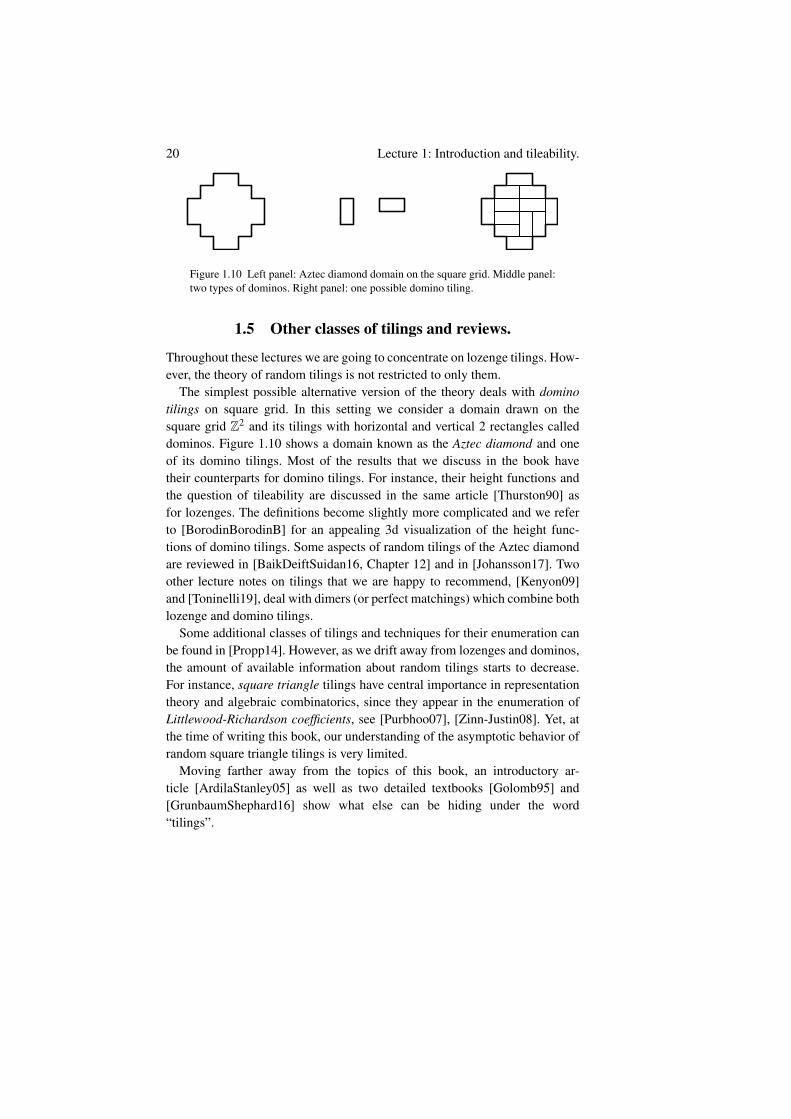
Figure 1.10 Left panel: Aztec diamond domain on the square grid. Middle panel:two types of dominos. Right panel: one possible domino tiling.
1.5 Other classes of tilings and reviews.
Throughout these lectures we are going to concentrate on lozenge tilings. How-ever, the theory of random tilings is not restricted to only them.
The simplest possible alternative version of the theory deals with dominotilings on square grid. In this setting we consider a domain drawn on thesquare grid Z2 and its tilings with horizontal and vertical 2 rectangles calleddominos. Figure 1.10 shows a domain known as the Aztec diamond and oneof its domino tilings. Most of the results that we discuss in the book havetheir counterparts for domino tilings. For instance, their height functions andthe question of tileability are discussed in the same article [Thurston90] asfor lozenges. The definitions become slightly more complicated and we referto [BorodinBorodinB] for an appealing 3d visualization of the height func-tions of domino tilings. Some aspects of random tilings of the Aztec diamondare reviewed in [BaikDeiftSuidan16, Chapter 12] and in [Johansson17]. Twoother lecture notes on tilings that we are happy to recommend, [Kenyon09]and [Toninelli19], deal with dimers (or perfect matchings) which combine bothlozenge and domino tilings.
Some additional classes of tilings and techniques for their enumeration canbe found in [Propp14]. However, as we drift away from lozenges and dominos,the amount of available information about random tilings starts to decrease.For instance, square triangle tilings have central importance in representationtheory and algebraic combinatorics, since they appear in the enumeration ofLittlewood-Richardson coefficients, see [Purbhoo07], [Zinn-Justin08]. Yet, atthe time of writing this book, our understanding of the asymptotic behavior ofrandom square triangle tilings is very limited.
Moving farther away from the topics of this book, an introductory ar-ticle [ArdilaStanley05] as well as two detailed textbooks [Golomb95] and[GrunbaumShephard16] show what else can be hiding under the word“tilings”.
Lecture 2: Counting tilings through de-terminants.
The goal of this lecture is to present two distinct approaches to the counting oflozenge tilings. Both yield different determinantal formulae for the number oftilings.
A statistical mechanics tradition defines a partition function as a total num-ber of configurations in some model or, more generally, sum of the weights ofall configurations in some model. The usual notation is to use capital letter Zin various fonts for the partition functions. In this language, we are interestedin tools for the evaluation of the partition functions Z for tilings.
2.1 Approach 1: Kasteleyn formula
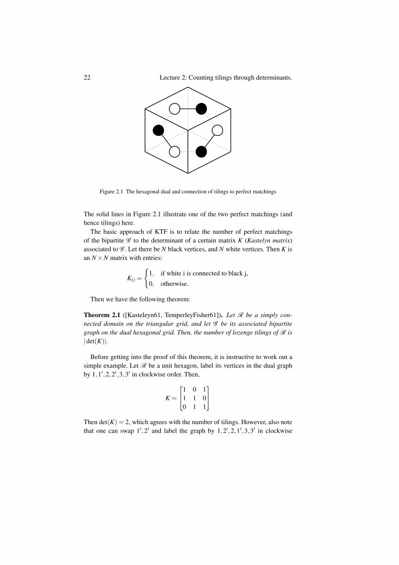
The first approach relies on what may be called “Kasteleyn theory” (or moreproperly “Kasteleyn-Temperley-Fisher (KTF) theory”), originally developedin [Kasteleyn61, TemperleyFisher61]. We illustrate the basic approach in Fig-ure 2.1 for lozenge tilings on the triangular grid. One may color the trianglesin two colors in an alternating fashion similar to a checkerboard. Connectingthe centers of adjacent triangles, one obtains a hexagonal dual lattice to theoriginal triangular lattice, with black and white alternating vertices. The graphof this hexagonal dual is clearly bipartite by the above coloring. Consider asimply connected domain R that consists of an equal number of triangles oftwo types (otherwise it can not be tiled), here we simply use a unit hexagon.Then lozenge tilings of it are in bijection with perfect matchings of the associ-ated bipartite graph (G ) formed by restriction of the dual lattice to the regioncorresponding to R, here a hexagon. As such, our question can be rephrased asthat of counting the number of perfect matchings of a (special) bipartite graph.
21
22 Lecture 2: Counting tilings through determinants.
Figure 2.1 The hexagonal dual and connection of tilings to perfect matchings
The solid lines in Figure 2.1 illustrate one of the two perfect matchings (andhence tilings) here.
The basic approach of KTF is to relate the number of perfect matchingsof the bipartite G to the determinant of a certain matrix K (Kastelyn matrix)associated to G . Let there be N black vertices, and N white vertices. Then K isan N×N matrix with entries:
Ki j =
1, if white i is connected to black j,
0, otherwise.
Then we have the following theorem:
Theorem 2.1 ([Kasteleyn61, TemperleyFisher61]). Let R be a simply con-nected domain on the triangular grid, and let G be its associated bipartitegraph on the dual hexagonal grid. Then, the number of lozenge tilings of R is|det(K)|.
Before getting into the proof of this theorem, it is instructive to work out asimple example. Let R be a unit hexagon, label its vertices in the dual graphby 1,1′,2,2′,3,3′ in clockwise order. Then,
K =
1 0 11 1 00 1 1
Then det(K) = 2, which agrees with the number of tilings. However, also notethat one can swap 1′,2′ and label the graph by 1,2′,2,1′,3,3′ in clockwise
23
order, resulting in:
K′ =
0 1 11 1 01 0 1
and det(K′) = −2. Thus, the absolute value is needed. This boils down to thefact that there is no canonical order for the black vertices relative to the whiteones.
Proof of Theorem 2.1 First, note that although there are N! terms in the de-terminant, most of them vanish. More precisely, a term in the determinant isnonzero if and only if it corresponds to a perfect matching: using two edgesadjacent to a single vertex corresponds to using two matrix elements from asingle row/column, and is not a part of the determinant’s expansion.
The essence of the argument is thus understanding the signs of the terms.We claim that for simply connected R (the hypothesis right now, subsequentlectures will relax it), all the signs are the same. We remark that this is a crucialstep of the theory; dealing with permanents (which are determinants withoutthe signs) is far trickier if not infeasible.
Given its importance, we present two proofs of this claim.
1 The first one relies on the height function theory developed in Lecture 1.Define elementary rotation E that takes the matching of the unit hexagon(1,1′),(2,2′),(3,3′) to (1,3′),(2,1′),(3,2′), i.e. swaps the solid and dash-dotted matchings in Figure 2.1. We may also define E−1. Geometrically, Eand E−1 correspond to removing and addding a single cube on the steppedsurface (cf. Lecture 1). We claim that any two tilings of R are connected bya sequence of elementary moves of form E,E−1. It suffices to show that wecan move from any tiling to the maximal tiling, i.e. the tiling correspondingto the point-wise maximal height function1. For that, geometrically one cansimply add one cube at a time until no more additions are possible. Thisprocess terminates on any simply connected domain R, and it can only endat the the maximal tiling.
It now remains to check that E does not alter the sign of a perfect match-ing. It is clear that the sign of a perfect matching is just the number ofinversions in the black to white permutation obtained from the matching(by definition of K and det). In the examples above, these permutations
1 The point-wise maximum of two height functions (that coincide at some point) is again aheight function, since the local rules (1.3) are preserved — for instance, one can show this byinduction in the size of the domain. Hence, the set of height functions with fixed boundaryconditions has a unique maximal element. In fact, we explicitly constructed this maximalelement in our proof of Theorem 1.4.
24 Lecture 2: Counting tilings through determinants.
are π(1,2,3) = (1,2,3) and π ′(1,2,3) = (3,1,2) respectively. (3,1,2) is aneven permutation, so composing with it does not alter the parity of the num-ber of inversions (i.e. the parity of the permutation itself). Thus, all perfectmatchings have the same sign.
2 The second approach relies upon comparing two perfect matchings M1 andM2 of the same simply connected domain R directly. We work on the dualhexagonal graph. Consider the union of these two matchings. Each vertexhas degree 2 now (by perfect matching hypothesis). Thus, the union con-sists of a bunch of doubled edges as well as loops. The doubled edges maybe ignored (they correspond to common lozenges). M1 and M2 are obtainedfrom each other by rotation along the loops, in a similar fashion to the opera-tion E above, except possibly across a larger number of edges. For a loop oflength 2p (p black, p white), the sign of this operation is (−1)p−1 as it cor-responds to a cycle of length p which has p−1 inversions. Thus it sufficesto prove that p is always odd.
Here we use the specific nature of the hexagonal dual graph. First, notethat each vertex has degree 3. Thus, any loop that does not repeat an edgecan not self intersect at a vertex, and is thus simple. Such a loop enclosessome number of hexagons. We claim that p has opposite parity to the total(both black and white) number of vertices strictly inside the loop. We provethis claim by induction on the number of enclosed hexagons. With a singlehexagon, p = 3, the number of vertices inside is 0 and the claim is trivial.Consider a contiguous domain made of hexagons P with a boundary oflength 2p. One can always remove one boundary hexagon such that it doesnot disconnect the domain P . Doing a case analysis on the position of thesurrounding hexagons, we see that the parity of the boundary loop length(measured in terms of say black vertices) remains opposite to that of thetotal number of interior vertices when we remove this hexagon. Hence, theclaim follows by induction.
It remains to note that the number of the vertices inside each loop is even.Indeed, otherwise, there would have been no perfect matchings of the inte-rior vertices2. Thus, p is always odd.
Remark 2.2. In general the permanental formula for counting perfect match-ings of a graph is always valid. However, to get a determinantal formulaone needs to introduce signs/factors into K. It turns out that one can alwaysfind a consistent set of signs for counting matchings of any planar bipar-tite graph. This is quite nontrivial, and involves the Kasteleyn orientation ofedges [Kasteleyn63, Kasteleyn67]. The hexagonal case is simple since one can
2 The assumption of the domain being simply-connected is used at this point.
25
use the constant signs by the above proof. For non-planar graphs, good choicesof signs are not known. However, for special cases, such as the torus that willbe covered in Lecture 3, small modifications of the determinantal formula stillwork. More generaly, on genus g surface, the number of perfect matchings isgiven by a sum of 22g signed determinants, cf. [CimasoniReshetikhin06] andreference therein. For non-bipartite graphs, one needs to replace determinantswith Pfaffians. Further information is available in, for instance, the work ofKasteleyn [Kasteleyn67], as well as the lecture notes on dimers [Kenyon09].
Exercise 2.3. Consider the domino tilings of the Aztec diamond, as in Figure1.10. Find out what matrix elements we should take for the Kasteleyn matrixK, so that its determinant gives the total number of tilings. (Hint: try to use the4th roots of unity: 1, −1, i, −i).
Remark 2.4. The construction that we used in the second proof of Theo-rem 2.1 can be turned into an interesting stochastic system. Take two inde-pendent uniformly random lozenge tilings (equivalently, perfect matchings)of the same domain and superimpose them. This results in a collection ofrandom loops which is known as the double-dimer model. What is happen-ing with this collection as the domain becomes large and the mesh size goesto 0? It is expected that one observes the Conformal Loop Ensemble CLEκ
with κ = 4 in the limit. For tilings of general domains this was not provenat the time when this book was written. However, partial results exist inthe literature and there is little doubt in the validity of this conjecture, see[Kenyon11, Dubedat14, BasokChelkak18].
2.2 Approach 2: Lindstrom-Gessel-Viennot lemma
Suppose we want to apply the above machinery to derive MacMahon’s formulafor the number of tilings of a R = A×B×C hexagon. In principle, we havereduced the computation to that of a rather sparse determinant. However, it isnot clear how we can proceed further. The goal of this section is to describe analternative approach.
We use a bijection of tilings with another combinatorial object, namely non-intersecting lattice paths as illustrated in Figure 2.2.
We describe the bijection as follows. Orient (without loss, consistentwith above orientation of hexagon) the three fundamental lozenges la, lb, lcwith their main diagonals pointing at angles 0, π
3 ,−π
3 . Leave la as is, anddraw stripes at angles π
6 ,−π
6 connecting the midpoints of opposite sidesof lozenges lb, lc respectively. There is thus a bijection between lozenge
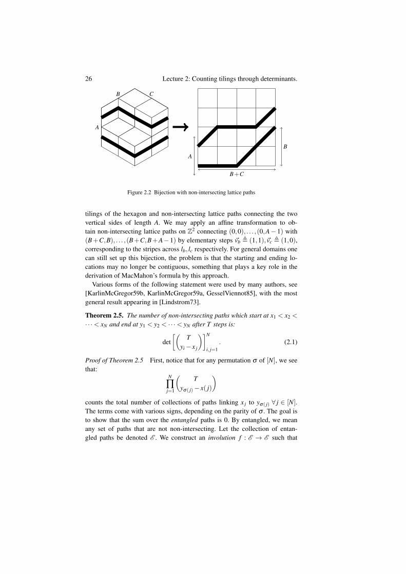
26 Lecture 2: Counting tilings through determinants.
A
B C
B+C
A
B
Figure 2.2 Bijection with non-intersecting lattice paths
tilings of the hexagon and non-intersecting lattice paths connecting the twovertical sides of length A. We may apply an affine transformation to ob-tain non-intersecting lattice paths on Z2 connecting (0,0), . . . ,(0,A− 1) with(B+C,B), . . . ,(B+C,B+A−1) by elementary steps ~vb , (1,1),~vc , (1,0),corresponding to the stripes across lb, lc respectively. For general domains onecan still set up this bijection, the problem is that the starting and ending lo-cations may no longer be contiguous, something that plays a key role in thederivation of MacMahon’s formula by this approach.
Various forms of the following statement were used by many authors, see[KarlinMcGregor59b, KarlinMcGregor59a, GesselViennot85], with the mostgeneral result appearing in [Lindstrom73].
Theorem 2.5. The number of non-intersecting paths which start at x1 < x2 <
· · ·< xN and end at y1 < y2 < · · ·< yN after T steps is:
det[(
Tyi− x j
)]N
i, j=1. (2.1)
Proof of Theorem 2.5 First, notice that for any permutation σ of [N], we seethat:
N
∏j=1
(T
yσ( j)− x( j)
)counts the total number of collections of paths linking x j to yσ( j) ∀ j ∈ [N].The terms come with various signs, depending on the parity of σ . The goal isto show that the sum over the entangled paths is 0. By entangled, we meanany set of paths that are not non-intersecting. Let the collection of entan-gled paths be denoted E . We construct an involution f : E → E such that
27
sign(σ( f (P))) = −sign(σ(P)) for all P ∈ E , where σ(P) denotes the per-mutation corresponding to which xi gets connected to which y j, and sign(σ)
denotes the parity of σ . This would complete the task, by the elementary:
2 ∑P∈E
sign(σ(P)) = ∑P∈E
sign(σ(P))+ ∑P∈E
sign(σ( f (P)))
= ∑P∈E
sign(σ(P))+ ∑P∈E−sign(σ(P))
= 0.
The involution is achieved by “tail-swapping”. Care needs to be taken to ensurethat it is well defined, as there can be many intersections. A simple choice is totake the first pair of indices i < j (in the sense of “leading vertex” coming fromx) paths that intersect, taking their rightmost intersecting point, and swappingtheir tails just beyond that. This is an involution, because the indices remainthe same when we iterate f , and swapping twice gets us back to where westarted. Furthermore, the parity of σ changes when we apply f . We note thatother choices are possible, as long as they are well-defined.
After cancellation, what we have left are non-intersecting paths. In the spe-cific setting here, they can only arise from σ being the identity, since any otherσ will result in intersections. The identity is an even permutation, so we do notneed to take absolute values here unlike the Kasteleyn formula.
Exercise 2.6. For a collection of paths E , let w(E ) denote the sum of verticalcoordinates of all vertices of all paths. Fix a parameters q, and using the samemethod find a q–version of (2.1). You should get a N×N determinantal for-mula for the sum of qw(E ) over all collections of non-intersecting paths startingat x1 < x2 < · · ·< xN and ending at y1 < y2 < · · ·< yN after T steps. At q = 1the formula should match (2.1).
We remark that for a general domain, we still do not know how to computethe determinant (2.1). However, if either xi or y j consist of consecutive integers,we can evaluate this determinant in “closed form”. This is true in the case ofthe A×B×C hexagon, and so we now prove Theorem 1.1.
By Theorem 2.5 and the bijection with tilings we described, we have reducedour task to the computation of:
det1≤i, j≤A
(B+C
B− i+ j
)(2.2)
Our proof relies upon the following lemma, which can be found in a veryhelpful reference for the evaluation of determinants [Krattenthaler99].
28 Lecture 2: Counting tilings through determinants.
Lemma 2.7. Let X1, . . . ,Xn,A2, . . . ,An,B2, . . . ,Bn be indeterminates. Then,
det1≤i, j≤n
((Xi +An)(Xi +An−1) . . .(Xi +A j+1)(Xi +B j)(Xi +B j−1) . . .(Xi +B2))
= ∏1≤i< j≤n
(Xi−X j) ∏2≤i≤ j≤n
(Bi−A j).
Proof The proof is based on reduction to the standard Vandermonde determi-nant by column operations. First, subtract the n− 1-th column from the n-th,the n−2-th from the n−1-th, . . . , the first column from the second, to reducethe LHS to:[
n
∏i=2
(Bi−Ai)
]det
1≤i, j≤n((Xi+An)(Xi+An−1) . . .(Xi+A j+1)(Xi+B j−1) . . .(Xi+B2)).
(2.3)Next, repeat the same process to the determinant of (2.3), factoring out
n−1
∏i=2
(Bi−Ai+1).
We can clearly keep repeating the process, until we have reached the simplifiedform: [
∏2≤i≤ j≤n
(Bi−A j)
]det
1≤i, j≤n((Xi +An)(Xi +An−1) . . .(Xi +A j+1)).
At this stage we have a slightly generalized Vandermonde determinant whichevaluates to the desired3:
∏1≤i< j≤n
(Xi−X j).
Proof of Theorem 1.1 Observe that:
det1≤i, j≤A
(B+C
B− i+ j
)=
[A
∏i=1
(B+C)!(B− i+A)!(C+ i−1)!
]
× det1≤i, j≤A
((B− i+A)!(B− i+ j)!
(C+ i−1)!(C+ i− j)!
)= (−1)(
A2)
[A
∏i=1
(B+C)!(B− i+A)!(C+ i−1)!
]
× det1≤i, j≤A
[(i−B−A)(i−B−A+1) · · ·(i−B− j−1)
× (i+C− j+1)(i+C− j+2) · · ·(i+C−1)].
3 Here is a simple way to prove the last determinant evaluation. The determinant is apolynomial in Xi of degree n(n−1)/2. It vanishes whenever Xi = X j and hence it is divisibleby each factor (Xi−X j). We conclude that the determinant is C ·∏i< j(Xi−X j) and it remainsto compare the leading coefficients to conclude that C = 1.
29
Now take Xi = i,A j =−B− j,B j =C− j+1 in Lemma 2.7 to simplify further.We get:
(−1)(A2)
[A
∏i=1
(B+C)!(B− i+A)!(C+ i−1)!
][∏
1≤i< j≤A(i− j)
][∏
2≤i≤ j≤A(C+B+1− i+ j)
]
=
[A
∏i=1
(B+C)!(B− i+A)!(C+ i−1)!
][∏
1≤i< j≤A( j− i)
][∏
2≤i≤ j≤A(C+B+1− i+ j)
]
=
[A
∏i=1
(B+C)!(B− i+A)!(C+ i−1)!
][∏
1≤ j<Aj!
][∏
2≤ j≤A
(C+B+ j−1)!(B+C)!
]
=
[A
∏i=2
1(B− i+A)!(C+ i−1)!
][∏
1≤ j<Aj!
][∏
2≤ j≤A(C+B+ j−1)!
](B+C)!
(B+A−1)!C!.
(2.4)
Perhaps the easiest way to get MacMahon’s formula out of this is to induct onA. This is somewhat unsatisfactory as it requires knowledge of MacMahon’sformula a priori, though we remark that this approach is common.
First, consider the base case A = 1. Then MacMahon’s formula is
B
∏b=1
C
∏c=1
b+ cb+ c−1
=B
∏b=1
b+Cb
=
(B+C
B
).
This is the same as the expression (2.4), as all the explicit products are empty.Keeping B,C fixed but changing A→ A+ 1, MacMahon’s formula multipliesby the factor:
B
∏b=1
C
∏c=1
A+b+ cA+b+ c−1
=B
∏b=1
A+b+CA+b
=(A+B+C)!(A+C)!
A!(A+B)!
.
Let us now look at the factor for (2.4). The numerator factors (A+B+C)!,A!arise from the right and middle explicit products in (2.4). The denominatorfactor (A+C)! arises from the denominator term (C + i− 1)! of (2.4). Theonly remaining unaccounted part of the denominator of (2.4) that varies withA is ∏
Ai=1
1(B+A−i)! , which thus inserts the requisite (A+B)! in the denominator
on A→ A+1. This finishes the induction and hence the proof.
30 Lecture 2: Counting tilings through determinants.
2.3 Other exact enumeration results
There is a large collection of beautiful results in the literature giving compactclosed formulas for the numbers of lozenge tilings4 of various specific do-mains. There is no unifying guiding principle to identify the domains for whichsuch formulas are possible, and there is always lots of intuition and guessworkinvolved in finding new domains (as well as numerous computer experimentswith finding the numbers and attempting to factorize them into small factors).
Once a formula for the number of tilings of some domain is guessed, apopular way for checking it is to proceed by induction, using the Dodgsoncondensation approach for recursive computations of determinants. This ap-proach relies on the Desnanot–Jacobi identity — a quadratic relation betweenthe determinant of a N×N matrix and its minors of sizes (N− 1)× (N− 1)and (N− 2)× (N− 2). The combinatorial version of this approach is knownas Kuo condesation, see e.g. [Ciucu15] and references therein. For instance,[Krattenthaler99] (following [Zeilberger95]) proves the Macmahon’s formulaof Theorem 1.1 in this way. Numerous generalizations of the Macmahon’s for-mula including, in particular, exact counts for tilings with different kinds ofsymmetries are reviewed in [Krattenthaler15]. One tool which turns out to bevery useful in enumeration of symmetric tilings is the matching factorizationtheorem of [Ciucu97].
Among other results, there is a large scope of literature devoted to ex-act enumeration of lozenge tilings of hexagons with various defects, seee.g. [Krattenthaler01, CiucuKrattenthaler01, CiucuFischer15, Lai15, Ciucu18,Rosengren16] and many more references therein. [Ciucu08] further used theformulas of this kind to emphasize the asymptotic dependence of tiling countson the positions of defects, which resembles the laws of electrostatics.
Some of the enumeration results can be extended to the explicit evaluationsof weighted sums over lozenge tilings and we refer to [BorodinGorinRains09,Young10, MoralesPakPanova17] for several examples.
4 While we only discuss lozenge tilings in this section, there are many other fascinating exactenumerations in related models. Examples include simple formulas for the number of dominotilings of rectangle in [TemperleyFisher61, Kasteleyn61] and of the Aztec diamond in[ElkiesKuperbergLarsenPropp92], or a determinantal formula for the partition function of thesix-vertex model with domain-wall boundary conditions of [Izergin87, Korepin82].
Lecture 3: Extensions of the Kasteleyntheorem.
3.1 Weighted counting
In the last lecture we considered tilings of simply connected regions drawnon the triangular grid by lozenges. If we checkerboard color the resulting tri-angles black and white, we saw that this corresponds to perfect matchings ofa bipartite graph G = (W tB,E). In this section we would like to extend theenumeration of matchings to the weighted situation.
The notational setup is as follows. Number the white and black vertices ofG by 1, 2, . . . , n. We regard the region R as being equipped with a weightfunction w(•)> 0 assigning to each edge i j ∈ E of G with white i and black jsome positive weight. Then we let the Kasteleyn matrix KR be an n×n matrixwith entries
KR(i, j) =
w(i j) i j is an edge of G
0 otherwise.
The difference with the setting of the previous lecture is that w(·) was identical1 there. When there is no risk of confusion we abbreviate KR to K. This matrixdepends on the labeling of the vertices, but only up to permutation of the rowsand columns, and hence we will not be concerned with this distinction.
By abuse of notation we will then denote to the weight of a tiling T by
w(T ) def= ∏
`∈Tw(`).
An extension of Theorem 2.1 states that we can compute the weighted sumof tilings as the determinant of the Kasteleyn matrix.
Theorem 3.1. The weighted number of tilings of a simply-connected domainR is equal to ∑T w(T ) = |detKR |.
31
32 Lecture 3: Extensions of the Kasteleyn theorem.
1′
2′
3′
2
1
3
w(2, 1)
w(1, 2)
w(3, 2)
w(3, 1)w(2, 3)
w(1, 3)
Figure 3.1 A unit hexagon with weights of edges for the corresponding graph.
The proof of Theorem 3.1 is the same as the unweighted case of countingthe number of tilings (obtained by setting w(i j) = 1 for each edge i j ∈ E) inTheorem 2.1. Let us remind the reader that simply-connectedness of R is usedin the proof in order to show that the signs of all the terms in the determinantexpansion are the same.
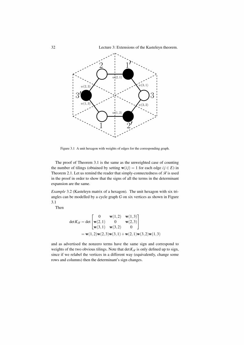
Example 3.2 (Kasteleyn matrix of a hexagon). The unit hexagon with six tri-angles can be modelled by a cycle graph G on six vertices as shown in Figure3.1
Then
detKR = det
0 w(1,2) w(1,3)w(2,1) 0 w(2,3)w(3,1) w(3,2) 0
= w(1,2)w(2,3)w(3,1)+w(2,1)w(3,2)w(1,3)
and as advertised the nonzero terms have the same sign and correspond toweights of the two obvious tilings. Note that detKR is only defined up to sign,since if we relabel the vertices in a different way (equivalently, change somerows and columns) then the determinant’s sign changes.
33
3.2 Tileable holes and correlation functions
There are situations in which the result of Theorem 3.1 is still true, even if R
is not simply connected.
Proposition 3.3. Suppose a region R is a difference of a simply connected do-main and a union of disjoint lozenges inside this domain. Let K be the Kaste-leyn matrix for R. Then the weighted sum of perfect matchings of R equals|detK|.
Proof Let R denote the simply connected region obtained by adding in theremoved lozenges. Then every nonzero term in detKR can be mapped intoa corresponding nonzero term in detK
Rby adding in the deleted lozenges.
We then quote the result that all terms in detKR
have the same sign, so thecorresponding terms in detKR should all have the same sign, too.
There is an important probabilistic corollary of Proposition 3.3. Let R beas in the proposition, and fix a weight function w(•) > 0. We can then speakabout random tilings by setting the probability of a tiling T to be
P(tiling T ) =1Z
w(T ) =1Z ∏
lozenge `∈Tw(`).
The normalizing constant Z = ∑T w(T ) is called the partition function.
Definition 3.4. Define the nth correlation function ρn as follows: givenlozenges `1, . . . , `n we set
ρn(`1, . . . , `n) = P(`1 ∈ T, `2 ∈ T, . . . , `n ∈ T ) .
The following proposition gives a formula for ρn.
Theorem 3.5. Write each lozenge as `i = (wi,bi) for i = 1, . . . ,n. Then
ρn(`1, . . . , `n) =n
∏i=1
w(wi,bi) deti, j=1,...,n
[K−1(bi,w j)
](3.1)
Remark 3.6. The proposition in this form was stated in [Kenyon97]. How-ever, the importance of the inverse Kasteleyn matrix was known since 60s, cf.[MontrollPottsWard63], [McCoyWu73].
34 Lecture 3: Extensions of the Kasteleyn theorem.
Proof of Theorem 3.5 Using Proposition 3.3, we have
ρn (`1, . . . , `n) =1Z ∑
tiling TT3`1,...,`n
∏`∈T
w(`)
=1Z
n
∏i=1
w(wi,bi)
∣∣∣∣ deti′, j′∈R\`1,...,`n
[K(wi′ ,b j′)
]∣∣∣∣=
n
∏i=1
w(wi,bi)
∣∣∣∣∣∣∣det
i′, j′∈R\`1,...,`n
[K(wi′ ,b j′)
]det
i′, j′∈R
[K(wi′ ,b j′)
]∣∣∣∣∣∣∣
=n
∏i=1
w(wi,bi) deti, j=1,...,n
[K−1(bi,w j)
],
where the last equality uses the generalizes Cramer’s rule (see e.g. [Prasolov94,Section 2.5.2]), which claims that a minor of a matrix is equal (up to sign) tothe product of the complimentary–transpose minor of the inverse matrix andthe determinant of the original matrix. In particular, the n = 1 case of thisstatement is the computation of the inverse matrix as the transpose cofactormatrix divided by the determinant:
K−1(bi,w j) = (−1)i+ jdet
i′, j′∈R\bi,w j[K(wi′ ,b j′)]
deti′, j′∈R
[K(wi′ ,b j′)].
Note that Proposition 3.3 involved the absolute value of the determinant. Weleave it to the reader to check that the signs in the above computation matchand (3.1) has no absolute value.
3.3 Tilings on a torus
Our next stop is to count tilings on the torus. The main motivation comes fromthe fact that translation-invariance of the torus allows as to use the Fourieranalysis to compute the determinants, which Kasteleyn theory outputs — thiswill be important for the subsequent asymptotic analysis. Yet, for non-planardomains (as torus), the Kasteleyn theorem needs a modification.
3.3.1 Setup
We consider a hexagonal grid on a torus T = S1× S1, again with the corre-sponding bipartite graph G = (W tB,E). The torus has a fundamental domain
35
n1 = 3
n2 = 3
(0, 0)
(0, 1)
(0, 2)
(1, 0)
(2, 0)
(2, 1)
(2, 2)
(1, 2)
(1, 1)
eβ eα
1
eβ(−1)a
eβ(−1)a
eβ(−1)a
eα(−1)b
eα(−1)b
eα(−1)b
Figure 3.2 An n1 × n2 = 3× 3 torus and its coordinate system. Three types ofedges have weights eα , eβ , and 1. When we loop around the torus, the weights getadditional factors (−1)a or (−1)b.
F drawn as a rhombus with n1 and n2 side lengths, as shown in Figure 3.2.We impose coordinates so that the black points are of the form (x,y) where0 ≤ x < n1 and 0 ≤ y < n2; see Figure 3.2. The white points have similar co-ordinates, so that black and white points with the same coordinate are linkedby a diagonal edge with white vertex being below. Our goal is to compute theweighted number of tilings, with a general weight function w(•).
As with the original Kasteleyn theorem, permK gives the number of perfect
36 Lecture 3: Extensions of the Kasteleyn theorem.
matchings, and our aim is to compute the signs of the terms when permanentis replaced by determinant.
To this end, we fix M0 the matching using only diagonal edges betweenvertices of the same coordinates — its edges are adjacent to coordinate labels((0,0), (0,1), etc) in Figure 3.2, and choose the numbering of the white andblack vertices so that the ith black vertex is directly above the ith white vertex.We let M be a second arbitrary matching of the graph. We would like to under-stand the difference between signs of M and M0 is detK. As before, overlayingM and M0 gives a 2-regular graph, i.e. a collection of cycles.
3.3.2 Winding numbers
The topological properties of the cycles (or loops) in M ∪M0 play a role infinding the signs of M and M0 in detM.
We recall that the fundamental group of the torus is Z×Z, which can beseen through the concept of the winding number of an oriented loop, which isa pair (u,v) ∈ Z×Z associated to a loop and counting the number of times theloop traverses the torus in two coordinate directions. In order to speak aboutthe winding numbers of the loops in M∪M0, we need to orient them in someway. This orientation is not of particular importance, as eventually only theoddity of u and v will matter for our sign computations.
For the nontrivial loops, we need the following two topological facts:
Proposition 3.7. [Facts from topology] On the torus,
• a loop which is not self-intersecting and not nullhomotopic has windingnumber (u,v) ∈ Z×Z with greatest common divisor gcd(u,v) = 1;
• any two such loops which do not intersect have the same winding number.
Both facts can be proven by lifting the loops to R2 — the universal cover ofthe torus — and analyzing the resulting curves there, and we will not providemore details here.
Proposition 3.8. Take all loops from M ∪M0, which are not double edges.Then each such loop intersects the vertical border of the fundamental domain(of Figure 3.2) u times and horizontal (diagonal) border of the fundamentaldomain v times for some (u,v) independent of the choice of the loop and withgcd(u,v) = 1. Further, the length of the loop, i.e. the number of black verticeson it, is n1u+n2v.
Proof Let γ denote one of the loops in question, and let us lift it to a path in
37
R2 via the universal cover
R2 S1×S1.
We thus get a path γ ′ in R2 linking a point (x,y) to (x+ n1u′,y+ n2v′) forsome integers u′ and v′. By Proposition 3.7, gcd(u′,v′) = 1 (unless u′ = v′ = 0)and u′, v′ are the same for all loops. Let us orient γ ′ by requiring that all theedges coming from M0 are oriented from black to white vertex. Then, sinceevery second edge of γ ′ comes from M0, we conclude that the x–coordinate isincreasing and the y–coordinate is decreasing along the path γ ′, i.e. the steps ofthis path of one oddity are (x′,y′)→ (x′,y′) and the steps of this path of anotheroddity are
(x′,y′)→ (x+1,y) or (x′,y′)→ (x,y−1), (3.2)
in the coordinate system of Figure 3.2. The monotonicity of path γ ′ impliesthat u′ = v′ = 0 is impossible, i.e. non-trivial loop obtained in this way can notbe null-homotopic. The same monotonicity implies u = |u′|, v = |v′| and thatthe length of the path is |n1u′|+ |n2v′|. The claim follows.
3.3.3 Kasteleyn theorem on the torus
In order to handle the wrap-around caused by the winding numbers u and v,we have to modify our Kasteleyn matrix slightly.
Fix the fundamental domain F as in Figure 3.2. We make the followingdefinition.
Definition 3.9. Let (a,b) ∈ 0,12. The Kasteleyn matrix Ka,b is the same asthe original K, except that
• For any edge crossing the vertical side of F with n1 vertices, we multiplyits entry by (−1)a.
• For any edge crossing the horizontal/diagonal side of F with n2 vertices,we multiply its entry by (−1)b.
Theorem 3.10. For perfect matchings on the n1×n2 torus we have
∑T
w(T ) =ε00 detK00 + ε01 detK01 + ε10 detK10 + ε11 detK11
2(3.3)
for some εab ∈ −1,1 which depend only on the parity of n1 and n2.
38 Lecture 3: Extensions of the Kasteleyn theorem.
Proof The correct choice of εab is given by the following table.
(n1 mod 2,n2 mod 2) (0,0) (0,1) (1,0) (1,1)ε00 −1 +1 +1 +1ε01 +1 −1 +1 +1ε10 +1 +1 −1 +1ε11 +1 +1 +1 −1
(3.4)
For the proof we note that each detKab is expanded as a signed sum of weightsof tilings and we would like to control the signs in this sum. For the matchingM0, the sign in all four Kab is +1. Since the sum over each column in (3.4) is 1,this implies that the weight of M0 enters into the right-hand side of (3.3) withthe desired coefficient 1.
Any other matching M differs from M0 by rotations along k loops of class(u,v), as described in Proposition 3.8. Note that at least one of the numbersu, v, should be odd, since gcd(u,v) = 1. The loop has the length n1u+ n2vand rotation along this loop contributes in the expansion of detKab the sign(−1)n1u+n2v+1+au+bv. Thus we want to show that the choice of εab obeys
1
∑a=0
1
∑b=0
εab · (−1)k(n1u+n2v+au+bv+1) = 2.
If k is even, then all the signs are +1 and the check is the same as for M0. Forthe odd k case, we can assume without loss of generality that k = 1 and weneed to show
1
∑a=0
1
∑b=0
εab · (−1)n1u+n2v+au+bv =−2.
We use the fact that u,v are not both even to verify that the choice (3.4) works.For example, if n1 and n2 are both even, then we get the sum
−1+(−1)u +(−1)v +(−1)u+v.
Checking the choices (u,v) = (0,1),(1,0),(1,1) we see that the sum is −2 inall the cases. For other oddities of n1 and n2 the proof is the same.
Remark 3.11. For the perfect matchings on a genus g surface, one would needto consider a signed sum of 22g determinants for counting, as first noticed in[Kasteleyn67]. For the detailed information on the correct choice of signs, see[CimasoniReshetikhin06] and references therein.
Exercise 3.12. Find an analogue of Theorem 3.10 for perfect matchings onn1×n2 cylinder.
Lecture 4: Counting tilings on largetorus.
This lecture is devoted to the asymptotic analysis of the result of Theorem 3.10.Throughout this section we use the eα , eβ weight for tilings as in Figure 3.2with a = b = 0.
4.1 Free energy
From the previous class we know that on the torus with side lengths n1 and n2,the partition function is
Z(n1,n2) = ∑Tilings
∏w(Lozenges)
=±K0,0 +±K1,0 +±K0,1 +±K1,1
2where Ka,b are the appropriate Kasteleyn matrices. Note that we can view Ka,b
as linear maps from CB to CW where B and W are the set of black and whitevertices on the torus.
Our first task is to compute the determinants detKab. The answer is explicitin the case of a translation-invariant weight function w. Choose any real num-bers α and β , and write
w(i j) ∈
1,eα ,eβ
according to the orientation of edge i j as in Figure 3.2. We evaluate
detKab = ∏eigenvalues Kab.
We start with K00 and note that it commutes with shifts in both directions.Since the eigenfunctions of shifts are exponents, we conclude that so should be
39
40 Lecture 4: Counting tilings on large torus.
the eigenfunctions of K00 (commuting family of operators can be diagonalizedsimultaneously). The eigenvalues are then computed explicitly, as summarizedbelow.
Claim 4.1. The eigenfunctions are given as follows: given input (x,y) ∈0, . . . ,n1−1×0, . . . ,n2−1 the eigenfunction is
(x,y) 7→ exp(
i · 2πkn1
x+ i · 2π`
n2y)
for each 0≤ k < n1, 0≤ ` < n2. The corresponding eigenvalue is
1+ eβ exp(−i
2πkn1
)+ eα exp
(i2π`
n2
).
Therefore the determinant of K0,0 is
n1
∏k=1
n2
∏`=1
(1+ eβ exp
(− i
2πkn1
)+ eα exp
(i2π`
n2
)).
For Ka,b we can prove the analogous facts essentially by perturbing theeigenvalues we obtained in the K0,0 case. The proof is straightforward andwe omit it.
Claim 4.2. Eigenvectors of Ka,b are
(x,y) 7→ exp(
i ·π 2k+an1
x+ i ·π 2`+bn2
y)
and the determinant of Ka,b is
n1
∏k=1
n2
∏`=1
(1+ eβ exp
(− iπ
2k+an1
)+ eα exp
(iπ
2`+bn2
)). (4.1)
Using this claim we find the asymptotic behavior of the (weighted) numberof possible matchings in the large scale limit.
Theorem 4.3. For the weights of edges
1,eα ,eβ
, as in Figure 3.2, we have
limn1,n2→∞
ln(Z(n1,n2))
n1n2=
"|z|=|w|=1
ln(|1+ eα z+ eβ w|) dw2πiw
dz2πiz
. (4.2)
Remark 4.4. The quantity ln(Z(n1,n2))n1n2
is known as the free energy per site.
Exercise 4.5. Show that the value of the double integral remains unchanged ifwe remove the | · | in (4.2).
41
Proof of Theorem 4.3 We first consider the case when eα + eβ < 1. In thiscase the integral has no singularities and we conclude that
limn1,n2→∞
ln(|detKa,b|)n1n2
=
"|z|=|w|=1
ln(|1+ eα z+ eβ w|) dw2πiw
dz2πiz
,
since the LHS is essentially a Riemann sum for the quantity on the right. Theonly possible issue is that upon taking the ± for each of a,b there may be amagic cancellation in Z(n1,n2) resulting in it being lower order. To see no suchcancelation occurs note that
maxa,b|detKa,b| ≤ Z(n1,n2)≤ 2max
a,b|detKa,b|.
The second inequality is immediate and follows from the formula for Z(n1,n2).The first one follows from noting that |detKa,b| counts the sets of weightedmatchings with ± values while Z(n1,n2) counts the weighted matchings un-signed. The result then follows in this case.
In the case when eα +eβ ≥ 1 we may have singularities; we argue that thesesingularities do not contribute enough to the integral to matter. The easiest wayto see this is to consider a triangle with side lengths 1,eα ,eβ . This gives twoangles θ ,φ which are the critical angles for singularity to occurs. However notethat πi( 2k+a
n1) cannot simultaneously be close for some k to the critical angle
φ for both a = 0 and a = 1. Doing similarly for θ it follows that there existsa choice of a,b where one can essentially bound the impact of the singularityon the convergence of the Riemann sum to the corresponding integral and theresult follows. (In particular one notices that roughly a constant number ofpartitions in the Reimann sum have |1+eα z+eβ w| close to zero and the aboveguarantees that you are at least≥ 1
max(n1,n2)away from zero so the convergence
still holds.)
4.2 Densities of three types of lozenges
We can use the free energy computation of the previous section to derive prob-abilistic information on the properties on the directions of the tiles in a randomtiling (or perfect matching). The probability distribution in question assigns toeach tiling (or perfect matching) T the probability
P(T ) =1
Z(n1,n2)∏
Lozenges in Tw(lozenge).
42 Lecture 4: Counting tilings on large torus.
Theorem 4.6. For lozenges of weight eα , we have
limn1,n2→∞
P(given lozenge is in tiling) ="|z|=|w|=1
eα z1+ eα z+ eβ w
dw2πiw
dz2πiz
.
(4.3)
Proof Using the shorthand # to denote the number of objects of a particulartype, we have
Z(n1,n2) = ∑Tilings
exp(α ·# +β ·# )
and therefore
∂
∂αlog(Z(n1,n2)) =
∑Tilings # · exp(α ·# +β ·# )
∑Tilings exp(α ·# +β ·# )
= E[# ]
= n1n2P(given lozenge is in tiling).
Therefore, using Theorem 3.10, we have
P(given lozenge is in tiling) = limn1,n2→∞
∂
∂αlog(Z(n1,n2))
= limn1,n2→∞
1n1n2
∂
∂α∑a,b=0,1±detKa,b
∑a,b=0,1±detKa,b
= limn1,n2→∞
∑a,b=0,1
∂
∂αdetKa,b
n1n2 detKa,b·
±detKa,b
∑a,b=0,1±detKa,b(4.4)
Ignoring the possible issues arising from the singularities of the integral, wecan repeat the argument of Theorem 4.3, differentiating with respect to α ateach step, to conclude that
limn1,n2→∞
∂
∂αdetKa,b
n1n2 detKa,b=
"|z|=|w|=1
eα z1+ eα z+ eβ w
dw2πiw
dz2πiz
, (4.5)
where the last expression can be obtained by differentiating the right-hand sideof (4.2). On the other hand, the four numbers
±detKa,b
∑a,b=0,1±detKa,b
have absolute values bounded by 1 and these numbers sum up to 1. Hence,(4.4) implies the validity of (4.3).
As in previous theorem, we have to address cases of singularities in the in-tegral in order to complete the proof of the statement. To simplify our analysis
43
we only deal with a sub-sequence of n1,n2 tending to infinity, along which(4.5) is easy to prove. The ultimate statement certainly holds for the full limitas well.
We use the angles θ and φ from the proof of Theorem 4.3. Define Wθ ⊆ Nas
Wθ =
n : min
1≤ j≤n
∣∣∣∣θ − π jn
∣∣∣∣> 1
n32
.
Define Wφ similiarly Note here that θ and φ are the critical angles coming fromtriangle formed by 1,eα ,eβ .
Lemma 4.7. For large enough n, either n or n+2 is in Wθ .
Proof Suppose that |θ − π jn | ≤
1
n32
and |θ − π j′n+2 | ≤
1
(n+2)32
. Note that for n
sufficiently large this implies that j′ ∈ j, j+1, j+2. However note that forsuch j and j′ it follows that∣∣∣∣π j
n− π j′
n+2
∣∣∣∣= O(
1n
)and thus for n sufficiently large we have a contradiction.
Now take n1 ∈Wφ and n2 ∈Wθ . Then note that the denominator (which weget when differentiating in α the logarithm of (4.1)) satisfies∣∣∣∣1+ eβ exp
(−i ·π 2k+a
n1
)+ eα exp
(i ·π 2`+b
n2
)∣∣∣∣≥Θ
(1
min(n1,n2)
)for all but a set of at most 4 critical (k, `) pairs. For these four critical pairs wehave that∣∣∣∣1+ eβ exp
(−i ·π 2k+a
n1
)+ eα exp
(i ·π 2`+b
n2
)∣∣∣∣≥Θ
(1
min(n1,n2)32
)as we have taken n1 ∈Wφ and n2 ∈Wθ . This bound guarantees that the appro-priate Riemann sum converges to the integral expression shown in (4.5).
Remark 4.8. Using the same proof as above one shows that
limn1,n2→∞
P(given lozenge is in tiling) ="|z|=|w|=1
11+ eα z+ eβ w
dw2πiw
dz2πiz
and
limn1,n2→∞
P(given lozenge is in tiling) ="|z|=|w|=1
eβ w1+ eα z+ eβ w
dw2πiw
dz2πiz
.
We introduce the notation for these probabilities as p , p , and the one inthe theorem statement as p .
44 Lecture 4: Counting tilings on large torus.
Definition 4.9. The (asymptotic) slope of tilings on the torus is (p , p , p ).
4.3 Asymptotics of correlation functions
The computation of Theorem 4.6 can be extended to arbitrary correlation func-tions. The extension relies on the following version of Theorem 3.5.
Theorem 4.10. Take a random lozenge tiling on the torus with arbitraryweights. Write n lozenges as `i = (wi,bi) for i = 1, . . . ,n. Then
P(`1, . . . , `N ∈ tiling)=∑a,b=0,1±detKab ∏
ni=1 Kab(wi,bi)det1≤i, j≤n K−1
ab (bi,w j)
∑a,b=0,1±detKab.
The proof here is nearly identical to the simply connected case. Then us-ing Theorem 4.10 as an input we can calculate the asymptotic nth correlationfunction.
Theorem 4.11. The nth correlation function in the n1,n2→ ∞ limit is
P((x1,y1, x1, y1), . . . ,(xn,yn, xn, yn) ∈ tiling)
=n
∏i=1
K00(xi,yi, xi, yi) det1≤i, j,≤n
(Kα,β [xi− x j, yi− y j]) (4.6)
where
Kα,β (x,y) ="|z|=|w|=1
wxz−y
1+ eα z+ eβ wdw
2πiwdz
2πiz. (4.7)
Note that in the above theorem (xi,yi) correspond to the coordinates of thewhite vertices while (xi, yi) correspond to the coordinates of the black vertices.The coordinate system here is as in Figure 3.2. Therefore (xi,yi, xi, yi) is simplyreferring to a particular lozenge.
Sketch of the proof of Theorem 4.11 Here is the plan of the proof:
• We know both the eigenvalues and eigenvectors for the matrix K and thisimmediately gives the same for the inverse matrix K−1.
• The key step in analyzing the asymptotic of the expression in Theorem 4.10is to write down the elements of matrix inverse as a sum of the coordinatesof eigenvectors multiplied by the inverses of the eigenvalues of K. As beforethis gives a Riemann sum approximation to the asymptotic formula shownin (4.7). Note that one can handle singularities in a manner similar to that ofTheorem 4.6 in order to get convergence along a sub-sequence.
45
• In more details, the normalized eigenvectors of Kab are
(x,y) 7→ 1√
n1n2exp(
i ·π 2k+an1
x+ i ·π 2`+bn2
y)
and the corresponding eigenvalues are
1+ eβ exp(−i 2πk+a
n1
)+ eα exp
(i 2π`+b
n2
)Now note that K−1
ab can be written as Q−1Λ−1Q where the columns of Q aresimply the eigenvectors of Kab and Λ the corresponding diagonal matrix ofeigenvalues. Note here Q−1 = Q∗ as Q corresponds to a discrete 2-D Fouriertransform. Substituting, it follows that
K−1ab (x,y;0,0) =
1n1n2
n1
∑k=1
n2
∑`=1
exp(i ·π 2k+a
n1x+ i ·πy 2`+b
n2y)
1+ eβ exp(−i 2πk+a
n1
)+ eα exp
(i 2π`+b
n2
)(4.8)
and the expressions in (4.7) appears as a limit of the Riemann sum of theappropriate integral. (Note K−1
ab (x,y;0,0) = K−1ab ((x+ x,y+ y; x, y)) as the
torus is shift invariant.)
Remark 4.12. The asymptotic of the free energy per site on n1 × n2 toruswas investigated for numerous models of statistical mechanics going well be-yond weighted tilings (which were investigated in the largest generality in[KenyonOkounkovSheffield03]). A widely used approach is to treat the torusas a sequence of n2 strips of size n1×1. One then introduces the transfer ma-trix T encoding the transition from a strip to the adjacent one and computesthe free energy as Trace(T n2). Hence, the computation reduces to the studyof eigenvalues of T and systematic ways for evaluations of these eigenvaluesare discussed in [Baxter82]. The answer is typically presented in terms of so-lutions to a system of algebraic equations known as Bethe equations. Findinganalytic expressions for the solutions of these equations (in the limit of largetorus) is a hard task, which is still mathematically unresolved in many situa-tions. From this perspective, tilings represent a specific “nice” case, in whichrelatively simple formulas of Theorems 4.3 and 4.11 are available.
Lecture 5: Monotonicity and concentra-tion for tilings
Last time we studied tilings on the torus, and now we go back to planar do-mains. The setup for this lecture is slightly different from before. We fix aboundary of our domain and values of a height function on the boundary, andconsider all height functions extending the given one. This is equivalent tostudying random tilings because we have a correspondence between heightfunctions (up to shifting by a constant) and tilings. The advantage of this setupis that we can compare height functions much easier than comparing tilingsdirectly. The material of this lecture is based on [CohnElkiesPropp96] and[CohnKenyonPropp00].
5.1 Monotonicity
We start with a domain R with boundary ∂R on the triangular grid. Recallthe three positive directions we defined in Lecture 1: (0,1), (−
√3
2 ,− 12 ), and
(√
32 ,− 1
2 ). Also recall that along an edge in the positive direction, the heightfunction changes by +1 if the edge is an edge of a lozenge; and the heightfunction changes by −2 if the edge crosses a lozenge. Fix a height functionh on ∂R. Note that if h changes by −2 on the boundary, then a lozenge ishalf outside R. Let us emphasize that this is a slightly different situation com-pared to the previous lectures, as the lozenges are allowed to stick out of R; inother words, we are now considering tilings not of R, but of another domainobtained by adding to R some triangles along the boundary ∂R.
Let us consider a height function H on R chosen uniformly randomly fromall height functions extending h. In the following, ∂R ⊆R can be any set ofvertices such that every vertex in R\∂R is adjacent only to vertices of R.
46
47
Proposition 5.1. Let R and ∂R be as above. Let h and g be two height func-tions on ∂R. Assume that h ≡ g (mod 3), h ≥ g and that h and g can beextended to height functions on R. Let H (resp. G) be a height function onR chosen uniformly randomly from all height functions extending h (resp. g).Then we can couple H and G in such a way that H ≥ G.
Remark 5.2. We require that h ≡ g (mod 3) because all height functions arethe same modulo 3 up to shifting by a global constant.
Proof of Proposition 5.1 We fix R and perform induction on |R\∂R|. Basecase is R = ∂R, where there is nothing to prove.
Suppose ∂R ( R. Choose a vertex v ∈ ∂R adjacent to w ∈R\∂R, suchthat h(v) > g(v). (If no such v can be chosen, then we can couple H and Gin such a way that H|R\∂R = G|R\∂R , and there is nothing to prove.) Let ussample H and G on R\∂R in two steps: First we sample H(w) and G(w), andthen we sample the rest.
Because h(v)> g(v) and h(v)≡ g(v) (mod 3), we have h(v)≥ g(v)+3. Setx= h(v)−2 and y= g(v)−2. The definition of the height function then impliesH(w) ∈ x,x+3 and G(w) ∈ y,y+3. Since x≥ y+3, we can couple H(w)and G(w) so that H(w)≥ G(w).
It remains to couple the values of H and G on R\(∂R ∪w) by inductionhypothesis.
Corollary 5.3. For any w ∈R, we have EH(w)≥ EG(w).
Remark 5.4. The proof of Proposition 5.1 extends from the uniform distribu-tion on height functions to more general ones. The only feature of the distri-bution that we used is the possibility of sequential (Markovian) sampling ofthe values of the height function, and the fact that the set of admissible valuesfor the height function at a point can be reconstructed by the value at a singleneighbor. Here is one possible generalization1.
Exercise 5.5. Prove an analogue of Proposition 5.1 for the measure on lozengetilings with weights 1
Z ∏w(lozenges), where w(·) is a positive function of typeof lozenge and its position; the product goes over all lozenges in a tilings andZ is a normalizing constant making the total mass of measure equal to 1.
1 Another generalization of tilings is the six-vertex model. The monotonicity property extendsonly to some particular cases of the latter, but not to the model with arbitrary parameters. Onthe level of the proofs, the difficulty arises because the weights of the six-vertex model aredetermined by the local configurations in squares (x,y), (x,y+1), (x+1,y), (x+1,y+1) andhence it is not enough to know h(x,y+1) and h(x+1,y) in order to sample h(x+1,y+1) —we also need h(x,y).
48 Lecture 5: Monotonicity and concentration for tilings
Similar generalizations to non-uniform distributions are possible for the fur-ther results in this lecture.
Proposition 5.6. Let R1 and R2 be two domains with boundaries ∂R1 and∂R2 resp. Let h be a height function on ∂R1 and let g be a height function on∂R2 such that h|∂R1∩∂R2 ≡ g|∂R1∩∂R2 (mod 3). Suppose that each vertex vof ∂R1 is within distance ∆1 from a vertex w in ∂R2, and vice versa, and foreach such pair of vertices, we have |h(v)− g(w)| ≤ ∆2. Then there exists anabsolute constant C > 0 such that
|EH(x)−EG(x)| ≤C(∆1 +∆2) for all x ∈R1∩R2,
where H (resp. G) is chosen uniformly randomly from height functions on R1
(resp. R2) extending h (resp. g).
Proof Let h be a minimal extension of h to R1, and g be a maximal ex-tension of g to R2. (They exist and are unique because pointwise maxi-mum or minimum of two height functions is again a height function.) Forany vertex v ∈ ∂ (R1 ∩R2) ⊆ ∂R1 ∪ ∂R2, the conditions imply that h(v) ≥g(v)−C(∆1 +∆2) for some absolute constant C > 0. Hence the same inequal-ity is true for any extension of h to R1 and g to R2. By Corollary 5.3, we getEH(x)≥ EG(x)−C(∆1 +∆2) for all x ∈R1∩R2. By swapping R1 and R2,we get EG(x)≥ EH(x)−C(∆1 +∆2).
Remark 5.7. In the proofs of this section we silently assumed that the exten-sions of the height functions from the boundaries exist. As long as this is true,we do not need to assume that the domains are simply connected.
5.2 Concentration
We proceed to the next question: how close is a random height function to itsexpectation?
Theorem 5.8. Let R be a connected domain with boundary ∂R. Let h be aheight function on ∂R. Let H be a uniformly random extension of h to R.Suppose that w,v ∈R are linked by a path of length m. Then
E(H(w)−E[H(w)|H(v)])2 ≤ 9m
and for each c > 0,
P(|H(w)−E[H(w)|H(v)]|> c
√m)≤ 2exp
(− c2
18
). (5.1)
49
Remark 5.9. If we choose as v a point for which the value of H(v) is determin-istically known (e.g., it can be a point on the boundary ∂R, then expectationsbecome unconditional and we get:
E(H(w)−E[H(w)])2 ≤ 9m
and for each c > 0,
P(|H(w)−E[H(w)]|> c
√m)≤ 2exp
(− c2
18
). (5.2)
Remark 5.10. If the linear size of the domain is proportional to L, then so isthe maximum (over w) possible value of m. Hence, (5.2) implies that as L→∞
the normalized height function H(Lx,Ly)L concentrates around its expectation.
We will soon prove that it converges to a limit, thus showing the existence of alimit shape for tilings.
Remark 5.11. It is conjectured that the variance should be of order O(logm),rather than O(m) which we prove. As of 2020, the tight bound was proved onlyfor some specific classes of domains.
Remark 5.12. Similarly to Exercise 5.5, the result extends to the measures ontilings with weight 1
Z ∏w(lozenges). The proof remains the same.
Proof of Theorem 5.8 Let x0 = v,x1, . . . ,xm = w be a path connecting v andw. Let Mk be the conditional expectation of H(w) given the values of H(x0),. . . , H(xk):
Mk = E[H(w) | H(x0),H(x1), . . . ,H(xk)
]In particular, M0 =E[H(w)|H(v)] and Mm =H(w). The tower property of con-ditional expectations implies that M0, . . . ,Mm is a martingale.
For fixed values of H(x0), . . . , H(xk), the random variable H(xk+1) takesat most two distinct values. Also, if H(xk+1) takes two values a < b, then wemust have b−a = 3. By Proposition 5.1, we have
E[H(w) | H(x0),H(x1), . . . ,H(xk); H(xk+1) = a
]≤ E
[H(w) | H(x0),H(x1), . . . ,H(xk); H(xk+1) = b
]≤ E
[H(w)+3 | H(x0),H(x1), . . . ,H(xk); H(xk+1) = a
].
(We get the second inequality by looking at the height function shiftedup by 3 everywhere.) Therefore E[H(w)|H(x0),H(x1), . . . ,H(xk)] and
50 Lecture 5: Monotonicity and concentration for tilings
E[H(w)|H(x0),H(x1), . . . ,H(xk+1)] differ by at most 3. Hence
E[(Mm−M0)2] = E
( ∑1≤k≤m
(Mk−Mk−1)
)2
= ∑1≤k,l≤m
E[(Mk−Mk−1)(Ml−Ml−1)]
= ∑1≤k≤m
E[(Mk−Mk−1)2]≤ 9m.
The third step is because E[(Mk −Mk−1)(Ml −Ml−1)] = 0 for k 6= l, bymartingale property (taking first the conditional expectation with respect toH(x0),H(x1), . . . ,H(xmin(k,l))).
The concentration inequality (5.1) follows from Azuma’s inequality appliedto the martingale Mk, see Lemma 5.13 below.
Lemma 5.13 (Azuma’s inequality [Azuma67]). Let X0, . . . ,XN be a martin-gale with |Xk−Xk−1| ≤ bk for all 1≤ k ≤ N. Then for each t > 0,
P(|XN−X0| ≥ t)≤ 2exp
(− t2
2∑Nk=1 b2
k
).
5.3 Limit shape
The results of the previous two sections say that random height functions con-centrates around their expectations, and the expectations continuously dependson the boundary conditions. The limiting profile, which we thus observe as thesize of the domain L tends to infinity is called the limit shape. So far, we do nothave any description for it, and our next aim is to develop such a description.Let us give a preview of the statement that we will be proving. The details arepresented in the several following lectures.
We can encode the gradient to (asymptotic) height function via proportionsof three types of lozenges , , . We then define (minus) surface tension to be
S(∇h) = S(p , p , p ) =1π(L(π p )+L(π p )+L(π p ))
where
L(θ) =−ˆ
θ
0log(2sin t)dt
is the Lobachevsky function.
51
Exercise 5.14. Assume that p , p , p are non-negative and satisfy p +
p + p = 1. Show that S(p , p , p ) vanishes whenever one of the argumentsvanishes and S(p , p , p )> 0 otherwise.
Theorem 5.15 (Variational principle, [CohnKenyonPropp00]). Consider a do-main R∗ with piecewise-smooth boundary ∂R∗. Let hb be a real function on∂R∗. Take a sequence of tileable, lattice domains RL with boundaries ∂RL
with scale depending linearly on L→ ∞. Fix a height function hL on ∂RL.Suppose that ∂RL
L → ∂R∗ and hLL converges to hb in sup norm.2 Then the
height function HL of a uniformly random tiling of RL converges in probabil-ity, in sup norm. That is, H(Lx,Ly)
L → hmax(x,y). Furthermore, hmax is the uniquemaximizer of the integral functional¨
R∗S(∇h)dxdy, h|∂R∗ = hb.
Simultaneously, we have
1L2 log(number of tilings of RL)→
¨R∗
S(∇hmax)dxdy. (5.3)
The proof of Theorem 5.15 is given at the end of Lecture 8 after we makesome preparatory work in the next two lectures.
2 Since the domain of definition of the function ∂hLL depends on L, one should be careful in
formalizing the sup-norm convergence. One way is to demand that for each ε > 0 there existsδ and L0, such that for all L > L0 and all pairs (x,y) ∈ ∂RL
L , (x∗,y∗) ∈ ∂R∗ satisfying|x− x∗|+ |y− y∗|< δ , we have
∣∣ 1L hL(Lx,Ly)−hb(x∗,y∗)
∣∣< ε .
Lecture 6: Slope and free energy.
We would like to asymptotically count the number of tilings for generic do-mains. The answer depends on the slope of the limit shape for random tilings,so we start with the fixed slope situation, where our computations for torus arehelpful.
6.1 Slope in a random weighted tiling
We work in the (α,β )-weighted setting, as in Lecture 4. Lozenges of typehas weight eβ , type has weight eα , and type has weight 1, where α,β ∈ R.In Theorem 4.6 and Remark 4.8 we computed the asymptotic slope of randomtilings on the torus:
p =
‹|z|=|w|=1
eβ w1+ eα z+ eβ w
dz2πiz
dw2πiw
,
p =
‹|z|=|w|=1
eα z1+ eα z+ eβ w
dz2πiz
dw2πiw
,
p =
‹|z|=|w|=1
11+ eα z+ eβ w
dz2πiz
dw2πiw
.
Let us evaluate one of these integrals, say, the second one computing p . Fix zand compute the w-integral
˛|w|=1
eα z1+ eα z+ eβ w
dw2πiw
.
The integrand has two poles, one at w= 0 and one at w=− 1+eα zeβ
. If both polesare in the contour, the w-integral has value 0 because we can let the contourgo to ∞, and the residue at ∞ is 0 because of O( 1
w2 ) decay. If w = − 1+eα zeβ
is
outside the contour, then the w-integral evaluates to eα z1+eα z by Cauchy’s integral
52
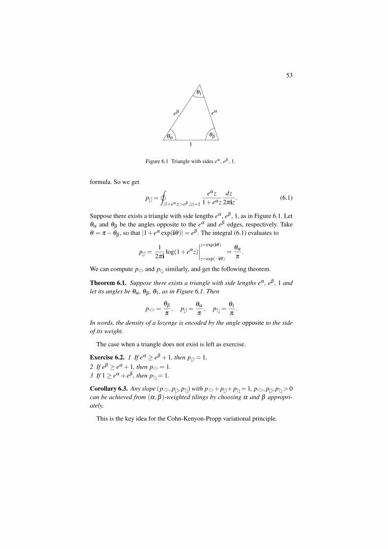
53
1
eαeβ
θαθβ
θ1
Figure 6.1 Triangle with sides eα , eβ , 1.
formula. So we get
p =
˛|1+eα z|>eβ ,|z|=1
eα z1+ eα z
dz2πiz
. (6.1)
Suppose there exists a triangle with side lengths eα , eβ , 1, as in Figure 6.1. Letθα and θβ be the angles opposite to the eα and eβ edges, respectively. Takeθ = π−θβ , so that |1+ eα exp(iθ)|= eβ . The integral (6.1) evaluates to
p =1
2πilog(1+ eα z)
∣∣∣∣z=exp(iθ)
z=exp(−iθ)=
θα
π.
We can compute p and p similarly, and get the following theorem.
Theorem 6.1. Suppose there exists a triangle with side lengths eα , eβ , 1 andlet its angles be θα , θβ , θ1, as in Figure 6.1. Then
p =θβ
π, p =
θα
π, p =
θ1
π.
In words, the density of a lozenge is encoded by the angle opposite to the sideof its weight.
The case when a triangle does not exist is left as exercise.
Exercise 6.2. 1 If eα ≥ eβ +1, then p = 1.2 If eβ ≥ eα +1, then p = 1.3 If 1≥ eα + eβ , then p = 1.
Corollary 6.3. Any slope (p , p , p ) with p + p + p = 1, p , p , p > 0can be achieved from (α,β )-weighted tilings by choosing α and β appropri-ately.
This is the key idea for the Cohn-Kenyon-Propp variational principle.
54 Lecture 6: Slope and free energy.
6.2 Number of tilings of a fixed slope
Now we compute the number of tilings of a torus of a fixed slope. Theorem4.3 computes the asymptotic of the number of tilings as a function of α andβ , while Theorem 6.1 relates α and β to the slope. So essentially all we needto do is to combine these two theorems together. We present a way to do itthrough the Legendre duality. We start from the setting of the finite torus inorder to see how this duality arises. (In principle, this is not strictly necessary,as one can analyze the formulas of Theorems 4.3, 6.1 directly.)
Say the torus has dimension n1× n2. Somewhat abusing the notations, wedefine the slope of a fixed tiling as
slope =1
n1n2(#lozenges of types( , , )).
(Previously, we thought of the slope only as a limit of this quantity as n1 andn2 tend to infinity.)
We have already computed the asymptotics of the partition function Z as afunction of α and β in Theorem 4.3. Z is related to the slope by
1n1n2
logZ =1
n1n2log ∑
slopeexp(α# +β# ) ·#tilings of this slope. (6.2)
Claim 6.4. 1 Under the (α,β )-measure, the distribution of slope as a randomvariable is concentrated as n1,n2→∞ around (p , p , p ), which we havecomputed. This is proved later in this lecture.
2 Asymptotics of the number of tilings depends continuously on the slope. Thisis proved in Lecture 8.
Using the claim, we have
1n1n2
logZ ≈ α p +β p +1
n1n2log#tilings of slope(p , p , p ). (6.3)
We define the surface tension as
σ(slope) = limn1,n2→∞
− 1n1n2
log#tilings of such slope.
(This will soon be shown to be the same as (−1) ·S, with S defined at the endof the last lecture.)
Let R(α,β ) be the limit of 1n1n2
logZ as n1,n2→ ∞. Then (6.3) gives
R(α,β ) = αs+β t−σ(s, t), (6.4)
where (s, t) are asymptotic values for the first two coordinates of the slope:
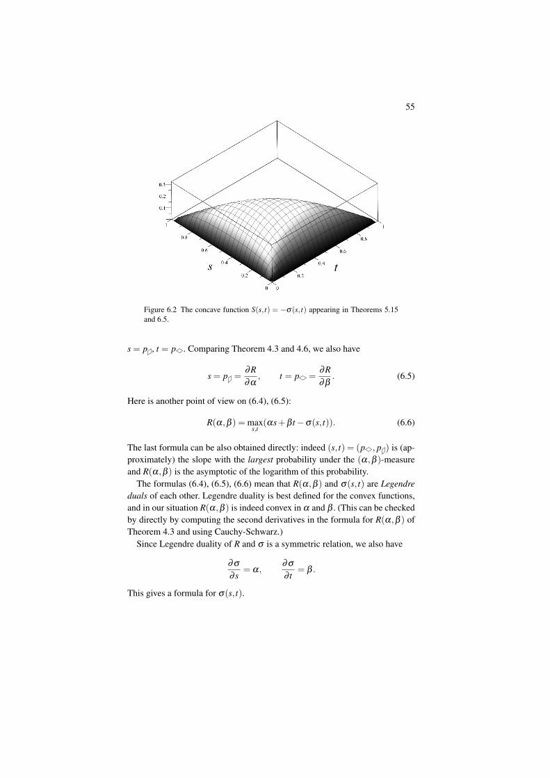
55
Figure 6.2 The concave function S(s, t) = −σ(s, t) appearing in Theorems 5.15and 6.5.
s = p , t = p . Comparing Theorem 4.3 and 4.6, we also have
s = p =∂R∂α
, t = p =∂R∂β
. (6.5)
Here is another point of view on (6.4), (6.5):
R(α,β ) = maxs,t
(αs+β t−σ(s, t)). (6.6)
The last formula can be also obtained directly: indeed (s, t) = (p , p ) is (ap-proximately) the slope with the largest probability under the (α,β )-measureand R(α,β ) is the asymptotic of the logarithm of this probability.
The formulas (6.4), (6.5), (6.6) mean that R(α,β ) and σ(s, t) are Legendreduals of each other. Legendre duality is best defined for the convex functions,and in our situation R(α,β ) is indeed convex in α and β . (This can be checkedby directly by computing the second derivatives in the formula for R(α,β ) ofTheorem 4.3 and using Cauchy-Schwarz.)
Since Legendre duality of R and σ is a symmetric relation, we also have
∂σ
∂ s= α,
∂σ
∂ t= β .
This gives a formula for σ(s, t).
56 Lecture 6: Slope and free energy.
Theorem 6.5. Under the identification s = p , t = p , we have
σ(s, t) =− 1π(L(πs)+L(πt)+L(π(1− s− t))) (6.7)
where L(θ) =−´
θ
0 log2sin t dt is the Lobachevsky function.
Proof When s = t = 0, both sides are equal to 0. σ(0,0) = 0 because there isexactly one tiling with slope (0,0,1). RHS is 0 is because L(0) = L(π) = 0.
Exercise 6.6. Prove that L(0) = L(π) = 0.
Let us compare the derivatives.
∂RHS∂ s
= log2sin(πs)− log2sin(π(1− t− s)) = α =∂σ
∂ s.
The second step is by the law of sines applied to the triangle with side lengthseα , eβ , 1. Similarly, we can show that
∂RHS∂ t
= β =∂σ
∂ t.
For the graph of the σ(s, t) function, see Figure 6.2.
Proposition 6.7. σ(s, t) is a convex function of (s, t) with s≥ 0, t ≥ 0, s+t ≤ 1.
Proof We can check this directly from formula 6.7. This also follows fromthe fact that σ(s, t) is the Legendre dual of R(α,β ).
6.3 Concentration of the slope
Now let us prove that the slope concentrates as n1,n2→ ∞.
Theorem 6.8. For the (α,β )–weighted random tilings of n1 × n2 torus,
limn1,n2→∞
|# −E# |n1n2
= 0 in probability.
Proof Let us compute the variance.
Var(# ) = Var
(∑
(x,y)∈torusI( at (x,y))
)= ∑
(x,y)∈torus∑
(x′,y′)∈torusCov(I( at (x,y)), I( at (x′,y′))).
(I(·) denotes the indicator function of an event.) If we show that Cov→ 0 as

57
|x− x′|, |y− y′| → ∞, then Var = o(n21n2
2) and concentration holds by Cheby-shev’s inequality. We have
Cov = P( at (x,y) and at (x′,y′))−P( at (x,y))P( at (x′,y′)).
By Theorem 4.11 of Lecture 4, as n1,n2→ ∞, the covariance goes to
e2β det(
Kα,β (1,0) Kα,β (x− x′+1,y− y′)Kα,β (x′− x+1,y′− y) Kα,β (1,0)
)− e2β Kα,β (1,0)2
(6.8)where
Kα,β (x,y) =‹|z|=|w|=1
wxz−y
1+ eα z+ eβ wdz
2πizdw
2πiw.
The double contour integral is a Fourier coefficient of a reasonably nice func-tion, so it goes to 0 as |x|, |y|→∞. Therefore, (6.8) also goes to zero, as desired.(Note that we use here slightly more than what is proved in Lecture 4. In Lec-ture 4, x−y′ and y−y′ are kept constant as n1,n2→∞. Here they should growwith n1,n2, so formally we have to deal directly with discrete Fourier coeffi-cients of (4.8) — but those still go to 0.)
6.4 Limit shape of a torus
We end this lecture by discussing how a random tiling of the torus looks likeon the macroscopic scale.
Take a fundamental domain of the torus. Let H = 0 at the bottom-left corner,and use paths only inside the fundamental domain to define height functionH(x,y) for the torus. By translation invariance, we have EH(x,y)−EH(x−1,y) = a and EH(x,y)−EH(x,y−1) = b, for all (x,y). Here (a,b) is a vectorwhich can be treated as a version of the slope. We conclude that EH(x,y) =ax+by.
Hence, using concentration inequality (5.2) from Lecture 5 (see Remark5.12), as L→ ∞ we have
supx,y
∣∣∣∣H(Lx,Ly)L
− (ax+by)∣∣∣∣→ 0
in probability. In other words, the limit shape for tilings is a plane.
Lecture 7: Maximizers in the variationalprinciple
7.1 Review
Recall the definitions of the Lobachevsky function
L(θ) =−ˆ
θ
0log(2sin t) dt.
and of the (minus) surface tension associated to a triple (p , p , p ) of densi-ties given by
S(p , p , p ) =1π
(L(π p )+L(π p )+L(π p )
).
The setup for the identification of the limit shape in the variational principleof Theorem 5.15 is as follows:
• For L→ ∞ we consider a sequence of finite domains RL, whose scale de-pends linearly in L, and fix a height function hL on each boundary ∂RL. Wesilently assume that hL is such that it has extensions to height functions onthe whole RL.
• As our target, we take a continuous region R∗ ⊆ R2 with piecewise smoothboundary ∂R∗, and let hb be a real function on this boundary.
We require the boundaries of RL to converge to those of the limiting regionR∗
1L
∂RL→ ∂R∗.
We do not need to specify the precise notion of convergence here, since thelimit shapes do not depend on the small perturbations of the boundaries (see
58
59
Lecture 5 and the following Lecture 8). Moreover, we require that
hL(Lx,Ly)L
→ hb(x,y) on ∂R∗,
which means that for each ε > 0 there exists δ > 0 and L0, such that for all L >
L0 and all pairs (x,y) ∈ ∂RLL , (x∗,y∗) ∈ ∂R∗ satisfying |x− x∗|+ |y− y∗|< δ ,
we have∣∣ 1
L hL(Lx,Ly)−hb(x∗,y∗)∣∣< ε .
The variational principle asserts (among other things) that a uniformly ran-dom height function HL of RL extending hL on ∂RL (=height function of auniformly random tiling) converges in probability to a function h∗ given by
h∗ = argmaxh∈H
¨R∗
S(∇h) dx dy (7.1)
In other words, the limit shape should be one that maximizes a certain surfacetension integral.
The goal of this lecture is to merely to make (7.1) precise (and subsequentlectures will actually prove the theorem). This means we need to make thefollowing steps:
• We define and motivate the class of function H mentioned in this maxi-mization problem.
• We define S(∇h) for h ∈H by associating a triple (p , p , p ) of localdensities to it.
• We prove that there exists a maximizing function h∗ across the choice of H .• We prove that the maximizing function is unique.
Throughout this lecture we retain R∗ as our target region with piecewisesmooth boundary ∂R∗. We fix the boundary function hb on ∂R∗ as well.
7.2 The definition of surface tension and class of functions
7.2.1 Identifying the gradient with the probability values
Let’s consider once again an h on a finite region. We can imagine walkingin the three directions indicated in Figure 7.1. Recall that the way our heightfunction h is defined, as we move in the +y direction we either get an incrementof +1 or −2 according to whether we cross a lozenge or not. Accordingly, inthe standard coordinate system with x-axis pointing to the right and y–axispointing up, we might colloquially write
∂h∂y
=−2p + p + p = 1−3p .
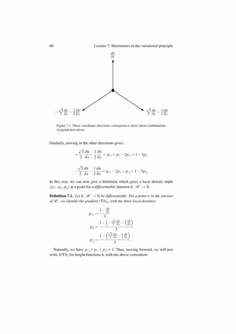
60 Lecture 7: Maximizers in the variational principle
∂h∂y
√3
2∂h∂x −
12
∂h∂y−
√3
2∂h∂x −
12
∂h∂y
Figure 7.1 Three coordinate directions correspond to three linear combinationsof partial derivatives.
Similarly, moving in the other directions gives:
+
√3
2∂h∂x− 1
2∂h∂y
= p + p −2p = 1−3p
−√
32
∂h∂x− 1
2∂h∂y
= p −2p + p = 1−3p .
In this way, we can now give a definition which gives a local density triple(p , p , p ) at a point for a differentiable function h : R∗→ R.
Definition 7.1. Let h : R∗→ R be differentiable. For a point w in the interiorof R∗, we identify the gradient (∇h)w with the three local densities
p =1− ∂h
∂y
3
p =1−(−√
32
∂h∂x −
12
∂h∂y
)3
p =1−(√
32
∂h∂x −
12
∂h∂y
)3
.
Naturally, we have p + p + p = 1. Thus, moving forward, we will justwrite S(∇h) for height functions h, with the above convention.
61
7.2.2 The desired set of functions
Next, we define the set of functions H we wish to consider: they are the func-tions h : R∗→ R which satisfy a Lipschitz condition so that p , p , p are inthe interval [0,1].
Definition 7.2. Let δ1,δ2,δ3 be unit vectors in the coordinate directions ofFigure 7.1. We denote by H the set of all functions
h : R∗→ R
such that:
(i) h agrees with hb (on ∂R∗)(ii) h satisfies the Lipschitz condition: for each i = 1,2,3 and ` > 0
−2≤ h((x,y)+ `δi)−h(x,y)`
≤ 1, (7.2)
where (x,y) and ` > 0 can be taken arbitrary as long as both (x,y) and(x,y)+ `δi belong to R∗.
Let us recall a general result about differentiability of Lipshitz functionsknown as the Rademacher theorem.
Theorem 7.3. A Lipschitz function is differentiable almost everywhere.
Whenever a function h ∈ H is differentiable at (x,y), the inequality(7.2) implies that the gradient encoded via Definition 7.1 by local densities(p , p , p ), satisfies 0≤ p , p , p ≤ 1.
We henceforth take as a standing assumption that H 6= ∅; this essentiallymeans that the boundary function hb should satisfy a similar Lipschitz condi-tion. (Which is automatically true if hb is obtained as a limit of height functionsof tileable regions.)
7.2.3 Goal
We have made all necessary definitions and the rest of this lecture is devotedto proving that there is a unique function h∗ ∈H which maximizes the valueof ¨
R∗S(∇h) dx dy.
62 Lecture 7: Maximizers in the variational principle
7.3 Upper semicontinuity
Definition 7.4. Let M be a metric space. A real-valued function f : M→ R isupper semicontinuous if for every point p, limsupx→p f (x)≤ f (p).
As the first step in proving the existence/uniqueness result, we prove thefollowing.
Theorem 7.5. Equip H with the uniform topology. Then over functions h ∈H , the function
h 7→¨
S(∇h) dx dy
is upper semicontinuous.
The proof relies on several lemmas.
Lemma 7.6. Let h∈H . Choose a mesh of equilateral triangles of side length`. Take a function h agreeing with h at vertices of each triangle, and linear oneach triangle (hence piecewise linear).
For each ε > 0, if ` > 0 is smaller than `0 = `0(ε), then for at least 1− ε
fraction of the triangles, the following holds:
• |h−h| ≤ `ε at each point inside the triangle,
• for (1−ε) fraction of the points of triangles, ∇h exists and∥∥∥∇h−∇h
∥∥∥< ε .
Outline of proof We mirror the proof of [CohnKenyonPropp00, Lemma 2.2].We first show that there is a 1− ε/3 fraction of triangles contained strictlywithin the region satisfying the first condition, and then proceed to the secondcondition. In both parts we implicitly use the Rademacher theorem implyingthat h is differentiable almost everywhere.
• First part: For every point of differentiability w, there exists a small realnumber r(w)> 0 such that
|h(w+d)−h(w)− (∇h)w ·d|<110
ε · |d|
for small displacements |d| ≤ r(p). If our mesh ` is so small that the set
w | r(w)> ` (7.3)
has measure at least (1− ε/3) · (AreaR∗), then (ignoring the triangles cutoff by the boundary), we can find a point w from the above set in each ofthe (1− ε/3) fraction of triangles. Thus, the linear approximation propertyholds on these triangles.
63
• For the second part we need to use the Lebesgue density theorem: Let a A beany Lebesgue measurable set, define the local density of A at x as
limε→0
mes(Bε(x)∩A)mes(Bε(x))
,
with Bε(x) being a ball of radius ε around x. Then the theorem (which wedo not prove here) claims that for almost every point x ∈ A the local densityequals 1.
Next, we choose finitely many sets U1, U2, . . . , Un covering all R∗ andsuch that whenever p,q ∈Ui, we have
∥∥(∇h)p− (∇h)q∥∥< ε/2 (this is pos-
sible since the space of possible gradients ∇h is compact). By applyingLebesgue’s density theorem to each of Ui, if ` is small enough, for pointw in all but ε/3 fraction of R∗, the value of ∇h in all but ε/3 fraction of theball of radius ` centered at w differs from (∇h)w at most by ε/2.
If w additionally belongs to the set (7.3) from the first part, then on thetriangle to which w belongs, ∇h differs from (∇h)w at most by ε/2. Hence,the second property holds.
Here is an immediate consequence of Lemma 7.6.
Corollary 7.7. Retaining the notation of the lemma,
limε→0
(¨R∗
S(∇h) dx dy−¨
R∗S(∇h) dx dy
)= 0.
The next lemma deals with very specific choices of R∗.
Lemma 7.8. Take as R∗ an equilateral triangle T of side length `. Let h ∈H
and choose a linear function h satisfying∣∣∣h− h
∣∣∣< ε` on ∂T . Then
˜T S(∇h) dxdy
AreaT≤
˜T S(∇h) dxdy
AreaT+o(1)
as ε → 0.
In other words we can replace h by its linear approximation if they agreealong the border of the domain T . Note that h is linear, rather than piecewiselinear — hence, this lemma is being applied to just one triangle T .
Proof of Lemma 7.8 By concavity of S, we have˜T S(∇h)dxdy
AreaT≤ S (Avg(∇h)) , (7.4)
where Avg(∇h) is the average value of ∇h on T . Also, we have∥∥∥Avg(∇h)−Avg(∇h)∥∥∥= O(ε),
64 Lecture 7: Maximizers in the variational principle
which can be proven by reducing the integral over T in the definition of theaverage value to the integral over ∂T using the fundamental theorem of thecalculus and then using
∣∣∣h− h∣∣∣< ε`. Therefore, by continuity of S,
S(Avg(∇h)) = S(Avg(∇h))+o(1).
Since h is linear, its gradient is constant on T and we can remove the averagevalue in the right-hand side of the last identity. Combining with (7.4) we getthe result.
Proof of Theorem 7.5 Let h ∈H . Then for each γ > 0 we want to show thatthere exists δ > 0 such that whenever g and h differ by at most δ everywhere,we should have ¨
R∗S(∇g)dxdy≤
¨R∗
S(∇h)dxdy+ γ
Take a piecewise linear approximation h for h from Lemma 7.6, and chooseδ < ε`. Let us call a triangle T of mesh “good”, if two approximation proper-ties of Lemma 7.6 hold on it. Then as ε → 0 we have by Lemma 7.8
¨T
S(∇g)≤¨
TS(∇h)+Area(T ) ·o(1)
and thus by summing over all the good triangles T¨
good triangles in R∗S(∇g)≤
¨good triangles in R∗
S(∇h)+Area(R∗) ·o(1).
Since S is bounded the bad triangles only add another O(ε). Thus, using alsoCorollary 7.7, we get
¨R∗
S(∇g)≤¨
R∗S(∇h)+Area(R∗) ·o(1).
7.4 Existence of the maximizer
The development of the previous section leads to the existence of maximizers.
Corollary 7.9. There exists a maximizer h∗ ∈H :
h∗ = argmaxh∈H
¨R∗
S(∇h)dxdy.
65
Proof We equip the set H with the uniform topology. It is then compact bythe Arzela-Ascoli theorem.
Let hn, n = 1,2 . . . , be a sequence of functions such that the integrals˜S(∇hn)dxdy approach as n → ∞ the supremum suph∈H
˜S(∇h)dxdy.
Passing to a convergent subsequence by compactness, we can assume with-out loss of generality that hn→ h∗, for some h∗ ∈H . Then, by Theorem 7.5
suph∈H
¨S(∇h)dxdy = limsup
n→∞
¨S(∇hn)dxdy≤
¨S(∇h∗)dxdy.
On the technical level, the difficulty in the proof of Corollary 7.9 is to passfrom uniform convergence of the functions to convergence of their gradients,which is necessary, since S is a function of the gradient. This was the mainreason for the introduction of the mesh of small equilateral triangles T in theprevious section.
7.5 Uniqueness of the maximizer
We end this lecture with a discussion of the uniqueness of maximizers.Let h1 and h2 be two maximizers (with the same value of the integral of S),
and let h = h1+h22 ∈H . Then using the concavity of S, we have
¨S(∇h)dxdy≥ 1
2
(¨S(∇h1)dxdy+
¨S(∇h2)dxdy
)=
¨S(∇h1)dxdy. (7.5)
If S(•) were strictly concave, the inequality in (7.5) would have been strict andthis would have been a contradiction with h1 6= h2 being two maximizers. An-noyingly, this is not quite true — S is only strictly concave in the region wherep , p , p > 0 (i.e. the interior of the triangle of possible slopes). Nonethelesswe would be done if there are points with ∇h1 6= ∇h2 with at least one of themstrictly inside the triangle of slopes.
Hence, the only remaining case is that all gradients ∇h1 and ∇h2 lie onthe boundary of the triangle of the slopes. Let us distinguish two kinds ofboundary slopes: extreme slopes, such that (p , p , p ) is either (1,0,0), or(0,1,0), or (0,0,1) and non-extreme boundary slopes where proportions oftwo types of lozenges are non-zero. Note that if h1 6= h2 are two maximizerswith all the slopes on the boundary, then passing to h = h1+h2
2 and using (7.5),if necessary, we would find a maximizer with non-extreme boundary slopes.However, we did not see any such slopes in the simulations shown in Figures
66 Lecture 7: Maximizers in the variational principle
1.3, 1.5 of Lecture 1. In fact, the following statement explains that non-extremeboundary slopes never appear in the limit shapes of tilings, as long as we tilenon-degenerate domains.
Proposition 7.10. If a domain R∗ with hb on ∂R∗ has at least one heightfunction h ∈H extending hb, such that all the slopes ∇h inside R∗ are noton the boundary of the triangle of possible slopes, then h with non-extremeboundary slopes (i.e. boundary slopes with non-zero proportions of preciselytwo types) cannot be a maximizer of
˜S.
Remark 7.11. For all the domains that we encounter in these lectures, the exis-tence of h is immediate. For instance, this is the case for tilings of polygonaldomains with sides parallel to the six grid directions of the triangular lattice.The only possible “bad” situation that we need to exclude is when the bound-ary conditions make some part of the tiling frozen (i.e. having only one type oflozenges) for every extension of hb — in this case we should simply removethis frozen part from the consideration and study the height functions in thecomplement.
Outline of the proof of Proposition 7.10 For ε > 0 consider¨R∗
[S(∇(εh+(1− ε)h))−S(∇h)] dxdy. (7.6)
We would like to study the small ε expansion of this difference by expandingthe integrand at each (x,y).
The explicit formula for S implies that the partial derivatives of S arebounded inside the triangle of slopes, but grow logarithmically at the boundary(except for the vertices (1,0,0), (0,1,0), (0,0,1)), cf. Figure 6.2.
Hence, the contribution to (7.6) of (x,y) with non-boundary (or extremeboundary) slopes of ∇h is O(ε). On the other hand, the contribution of (x,y)with non-extreme boundary slopes is of order ε logε ε , since the definitionof h implies that ∇(εh+(1− ε)h) is strictly inside the triangle of slopes forany ε > 0. Simultaneously, this contribution is positive for all (x,y), since Shas a minimum on the border of the triangle, cf. Figure 6.2. Hence, (7.6) ispositive for small ε contradicting the maximality of the integral for h.
Another proof for the uniqueness of maximizers can be found in[DeSilvaSavin08, Proposition 4.5].
Lecture 8: Proof of the variational prin-ciple.
In this lecture, using the machinery we have set up, prove the variational prin-ciple of Theorem 5.15 following [CohnKenyonPropp00].
Proposition 8.1. Let R be a convex region in the plane, and fix positive realsk,ε . Suppose that R fits within some L×L square, where L> ε−1, and supposeit has area A≥ kL2.
Let hb be a height function on ∂R which is within εL of the height functionof a fixed plane Π. Then, the quantity:
1A
ln(# of extensions of hb to R) (8.1)
is independent of the choice of hb (but depends on Π) up to an additive errorof O(ε1/2 log 1
ε), which might depend on k.
Proof The proof splits into two cases depending on the slope of Π.Case 1: The slope of Π is at least ε1/2 away from any boundary slope; in
other words, the proportion of each lozenge corresponding to the slope of Π isat least ε1/2 and at most 1− ε1/2.
Take a height function gb (on ∂R) also agreeing with the plane Π; we willshow that the values of (8.1) for gb and hb are within O(ε1/2 log 1
ε) of each
other.Assume gb≥ hb; if not, then we can compare both gb,hb with min(gb,hb) in-
stead. Let g∗,h∗ denote the minimal extension of gb and the maximal extensionof hb to R, respectively (since maximum/minimum of two height functions isagain a height function, such extensions are uniquely defined). We define twomaps that operate on height functions on R. If f is an extension of gb to R,then we define H( f ) to be the extension of hb to R given by the pointwise
67
68 Lecture 8: Proof of the variational principle.
minimum:
H( f ) = min( f ,h∗)
Similarly, if f is an extension of hb to R, then G( f ) is the extension of gb toR given by:
G( f ) = max( f ,g∗)
Note that H(G( f )) = f at all points in R at which the value of f is betweeng∗ and h∗ (in that order).
Recall the formula for h∗ in terms of hb from Leacture 1 (for g∗ the formulais similar):
h∗(x) = minu∈∂R
(d(x,u)+hb(u)),
where d is the distance function within R. Note that since R is convex, d is dif-fers (up to a small error) by a constant factor from the Euclidean distance in theplane. Thus, g∗ and h∗ differ from the height of Π by at least Ω(ε1/2d(x,∂R)),since the slope of Π is at least ε1/2 away from any boundary slope.
On the other hand, we claim that a typical random extension of hb to R isclose to Π. Indeed, to see that we embed R into a torus and consider a random(α,β )–weighted tiling of the torus, where α and β are chosen so that the limitshape of such a random tiling has slope Π, cf. Lecture 6. The concentrationof the height function of Lecture 5 applied to the torus means that hb is closeon ∂R to the height function of random tiling of the torus. We can then com-pare random extension of hb to a random tiling of the torus conditional on thevalues of its height function on ∂R. Note that the conditioning removes non-uniformity, i.e. the conditional law of (α,β )–weighted tilings on the torus isthe same as for the uniformly random tilings1 Hence, we can use the argumentsof Lecture 5. In particular, Proposition 5.1 (see also Proposition 5.6) impliesthat with probability tending to 1 (as the size of the domain grows), the heightfunction of random extension of hb is close to that of a random tiling of thetorus, which is close to Π.
We conclude that with high probability, a random extension of hb to R is adistance at most εL from Π. Thus, we have that for random extension f of hb,with probability approaching 1, H(G( f )) = f at all points at a distance at least
1 In order to see the conditional uniformity, notice that as soon as we know the values of theheight function on ∂R, we know the total number of lozenges of each of the three types insideR. Indeed, all the tilings with fixed boundary condition can be obtained from each other byadding/removing unit cubes, as in the first proof of Theorem 2.1, and each such operationkeeps the number of lozenges of each type unchanged. Hence, the each lozenge tiling of Rwith fixed values of the heights on ∂R has the same (α,β )-weight.
69
ε1/2(log 1ε)L from the boundary ∂R. This gives a partial bijection between
extensions of hb and extensions of gb.It remains to deal with the points at a distance less than ε1/2(log 1
ε)L from
the boundary ∂R. The possible values of the height function at these pointscan be constructed sequentially: when we move from a point to its neighborthere are two possible choices for the value of the height function. Thus, notingthat there are O(ε1/2(log 1
ε)L2) points close to the boundary ∂R, the number of
extensions of g and h differ by a multiplicative factor of at most 2O(ε1/2(log 1ε)L2),
as desired.Case 2: The slope of Π is within ε1/2 of some boundary slope; in other
words, the proportion of some type of lozenges, p , p , or p , is at most ε1/2.Without loss of generality, assume that the probability of a horizontal lozengeis p < ε1/2. Let us show that in this case, (8.1) is close to 0.
Consider some extension of hb, and consider all the vertical sections of R
by straight lines. Note that we know the number of horizontal lozenges onthese lines exactly, by calculating the change in the value of hb on each of theselines. This number is O(ε1/2L) due to hb being close to Π on ∂R. Thus, thetotal number of lozenges inside R is at most O(ε1/2L2). Note that the posi-tions of lozenges uniquely determine the rest of the tiling, i.e. the lozengesof the other two types. Thus the number of tilings is at most the number ofarrangements of lozenges, which is at most (where c is the constant in thebig O):
(A
cε1/2L2
)≤ Acε1/2L2(
cε1/2L2
e
)cε1/2L2 ≤
(L2
cε1/2L2
e
)cε1/2L2
=
(e
cε1/2
)cε1/2L2
= exp(L2O(ε2 log 1ε)).
Corollary 8.2. In the setting of Proposition 8.1, if R is an L by L square, then:
1A
ln(# of extensions of h to R) = S(slope of Π)+O(ε2 log 1ε) (8.2)
Proof Let us embed L×L square into L×L torus. If we deal with randomtilings of this torus, then the height function on the boundary of our squareis now random. However, in Section 6.4 we have shown this height functionis asymptotically planar. Hence, using Proposition 8.1 we conclude that thenumber of tilings of the square is approximately the same as the number of the
70 Lecture 8: Proof of the variational principle.
fixed slope tilings of the torus2 The asymptotic of the latter was computed inTheorem 6.5.3
Proposition 8.3. The statement (8.2) still holds when R is an equilateral tri-angle.
Proof Tile R with small squares, so that every square is completely containedwithin R (a small portion of R will be uncovered, but this is negligible so weignore it). Fix a (consistent) height function that is within O(1) of the planeon the boundaries of the squares. Note that, given this height function on theboundaries of the squares, a tiling of each of the squares yields a valid tiling ofR. Therefore,
1A
ln(# of tilings of R)≥ 1A
ln(# of tilings of all squares)
=1A ∑
squares sln(# of tilings of s)
≥ 1A ∑
squares sArea(s)(S(slope of Π)+O(ε2 log 1
ε))
= S(slope of Π)+O(ε2 log 1ε)
Now, for the other direction of the inequality, we will use an identical argu-ment; tile a large square with (approximately) equal numbers of copies of R
and R ′ (a vertically flipped copy of R). Then, each tiling of the square yieldsa tiling of each triangle, so we have:
∑copies of R,R ′
ln(# of tilings)≤ (total area) ·S(slope of Π)+O(ε2 log 1ε).
Noting that the lower bound applies for both R and R ′ parts of the last sum,we obtain the desired bound.
The final ingredient of the proof of the variational principle, is contained inthe following theorem:
Theorem 8.4. Let R∗ be a region with a piecewise smooth boundary, and leth∗b be a continuous height function on ∂R∗. Further, let R = RL be a latticeregion with a height function hb on ∂R, and for some fixed δ , suppose that
2 We also need to sum over all possible choices of the approximately planar heights on theboundary of the square. However, the number of such choices is exp(O(L)) and we can ignorethis factor in computation, since we only care about the leading O(L2) asymptotics of thelogarithm of number of extensions.
3 Theorem 6.5 relies on Theorem 4.3, which was proven only for tori of specific sizes. However,the sizes form a positive-density subset and thus it suffices to use only those sizes.
71
1LR is within δ of R∗ and 1
L hb is within δ of h∗b. Suppose also that there existextensions of hb to R.
Then, given a function h∗ ∈H which agrees with h∗b on ∂R∗, we have:
1L2 ln(number of extensions of hb to R within Lδ of Lh∗)
=
¨S(∇h∗)dxdy+o(1) (8.3)
in the limit regime when we first send L→ ∞ and then δ → 0. The remaindero(1) is uniform over the choice of h∗.
Proof Pick arbitrary (small) ε > 0. Pick `= `(ε) as in Lemma 7.6 in Lecture7 and create an `-mesh of equilateral triangles on the region 1
LR. We will takeδ < `ε . Let h be a height function which agrees with h∗ on the vertices of themesh and is piecewise linear within each triangle of the mesh. By Lemma 7.6on all but an ε fraction of the triangles, the function h is within ε` of h∗ on theboundaries of the triangle.
Note that we can ignore the ε fraction of “bad” triangles, since the contri-bution from these to (8.3) is negligible as ε → 0. The negligibility is based onthe observation that for each bad triangle there is at least one discrete heightfunction extending to the entire triangle the values of Lh∗ on the vertices ofthis triangle in such a way that it stays within Lδ of Lh∗. On the other hand,the total number of such extensions is at most exp(O(area of the triangle)).
Now, in order to lower bound the LHS of (8.3), note that we can obtain avalid extension of hb to R by first fixing the values at the vertices of the mesh toagree with h∗, then choosing the values of the height function on the boundariesof the triangles in an arbitrary way (but keeping them close to the piecewise-linear approximation h), and finally, counting all possible extensions from theboundary of the triangles of the mesh to the interior. Using Proposition 8.3 weget an estimate for the total number of tilings constructed in this way, whichmatches the RHS of (8.3). The overwhelming majority of the height functionsof these tilings is in Lδ–neighborhood of Lh∗, since we chose them in such away of the boundaries of the triangles and then can use the comparison withtorus, as in the proof of Proposition 8.1 to conclude that the height function isclose to h inside the triangles. Since h is close to h∗ by the construction, thedesired lower bound is obtained.
For the upper bound of the RHS of (8.3), we take an arbitrary tiling of R
with height function h and restrict it to each triangle in the mesh; note that thismust yield a valid tiling of each good triangle. Thus, summing over all possibleboundary conditions on sides of the triangles of the mesh (whose normalized
72 Lecture 8: Proof of the variational principle.
heights must be within `ε of h∗, since δ < `ε) and using Proposition 8.3 foreach triangle, we obtain the desired upper bound. It is crucial at this step thatthe number of choices of all possible boundary conditions on the sides of thetriangles grows as exp(o(L2))4 and is therefore negligible for (8.3).
Remark 8.5. One might want to be slightly more careful near the boundariesof the domain, since h∗ might be not defined in the needed points. We donot present these details here and refer to [CohnKenyonPropp00]. We also donot detail uniformity of the remainder o(1), leaving this as an exercise to thereaders.
Proof of Theorem 5.15 For a function h∗ ∈H and δ > 0, let Uδ (h∗) denotethe set of all functions h from H , for which sup(x,y)∈R∗ |h(x,y)−h∗(x,y)|< δ .
Let hmax be the maximizer of Corollary 7.9. Choose an arbitrary small ε > 0.Using uniqueness of maximizer, compactness of H , and Theorem 7.5, we canfind δ0 (depending on ε), such that¨
R∗S(∇h)dxdy <
¨R∗
S(∇hmax)dxdy− ε,
for each h ∈H outside Uδ0(hmax).
Note that the choice δ0 = δ0(ε) can be made in such a way that δ0 → 0 asε→ 0. Next, choose another δ > 0, so that o(1) in (8.3) is smaller in magnitudethan ε/2. This δ can be arbitrary small and therefore we can require withoutloss of generality that δ < δ0.
Using compactness of the space H , we can now choose finitely manyelements h∗1, . . . ,h
∗k ∈ Uδ0(h
max) with h∗1 = hmax and finitely many elementsh∗k+1, . . . ,h
∗m ∈H \Uδ0(h
max), so that (for large L) each height function HL ofa tiling of RL is in δL–neighborhood from one of the functions Lh∗i , 1≤ i≤m.The numbers k, m and functions h∗1, . . . ,h
∗m depend on ε and δ , but not on L.
Let Ni, 1 ≤ i ≤ m denote the number computed in (8.3) for h∗ = h∗i . Thenwe have a bound
exp(L2N1)≤ number of extensions of hb to RL ≤m
∑i=1
exp(L2Ni) (8.4)
Sending L→ ∞ using (8.3) and the fact that h∗1 = hmax is the maximizer, we
4 There are O(`−2) triangles in the mesh and each of them has sides of length O(`L). Hence, thetotal length of all sides of the triangles of the mesh is O(`−1 ·L). If we define heights along thesides of triangles sequentially, starting from the boundary of the domain (where they arefixed), then when we move to an adjacent vertex of the grid, we choose from at most 2possible values of the height function. Hence, the total number of possible values for theheight function on all sides of all triangles can be upper-bounded by 2O(`−1 ·L).
73
get¨
R∗S(∇hmax)dxdy−ε/2≤ lim
L→∞
1L2 ln(number of extensions of hb to RL)
≤¨
R∗S(∇hmax)dxdy+ ε/2 (8.5)
Since ε > 0 is arbitrary, this proves (5.3).Further, using δ < δ0, we can write
1−P(HL is within 2Lδ0 from hmax)≤ ∑mi=k+1 exp(L2Ni)
exp(L2N1)(8.6)
Using (8.3) and definition of δ0 we conclude that the numerator in (8.6) isupper-bounded by
(m− k)exp(
L2(¨
R∗S(∇hmax)dxdy− ε/2
)+o(L2)
).
Simultaneously, the denominator is lower-bounded using (8.3) by
exp(
L2¨
R∗S(∇hmax)dxdy+o(L2)
).
We conclude that the ratio in (8.6) goes to 0 as L→ ∞. Since δ0 can be madearbitrary small as ε → 0, this implies convergence in probability 1
L H → hmax.
Lecture 9: Euler-Lagrange and Burgersequations.
In the previous lectures we reduced the problem of finding a limit shape ofrandom tilings to a variational problem. Now we start discussing ways to solvethe latter.
9.1 Euler-Lagrange equations
Recall that the limit shape of a tiling, under certain conditions, is:
argmaxh
¨S(∇h)dxdy.
We will consider the general problem of finding
argmaxh
¨F(hx,hy,h)dxdy (9.1)
for a general function F of three real arguments (and we are going to plug in hx
as the first argument, hy as the second argument, and h as the third argument).
Proposition 9.1 (Euler-Lagrange equations). For maximal h(x,y) solving(9.1), at all points (x,y) where h is smooth (as a function of (x,y)) andF(hx,hy,h) is smooth (as a function of its argument in a neighborhood of(hx(x,y),hy(x,y),h(x,y))), we have:
∂
∂x
(F1(hx,hy,h)
)+
∂
∂y
(F2(hx,hy,h)
)−F3(hx,hy,h) = 0 (9.2)
where Fi denotes the derivative of F in its i-th argument.In the non-coordinate form, the first two terms can be written as div(∇F
∇h), representing the divergence of the vector field ∇F evaluated at ∇h(x,y).
74
75
Proof Note that since h is maximal, we must have, for all smooth g,
∂
∂ε
(¨F((h+ εg)x,(h+ εg)y,(h+ εg))dxdy
)∣∣∣∣ε=0
= 0
Using the Taylor series expansions of F , this reduces to:¨
(F1(hx,hy,h)gx +F2(hx,hy,h)gy +F3(hx,hy,h)g) dxdy = 0
Now pick g to be smooth with compact support strictly inside the domain andintegrate by parts in x in the first term and in y in the second term to get:
¨ (∂
∂x(F1(hx,hy,h))+
∂
∂y(F2(hx,hy,h))− (F3(hx,hy,h))
)gdxdy = 0.
Since g is arbitrary, the first factor in the integrand has to vanish.
Specializing Euler-Lagrange equations to our functional S(∇h) we see twodifferent situations:
• If ∇h at a point (x,y) lies strictly inside of the triangle of possible slopes,then (9.2) is a meaningful equation at this point.
• If ∇h is a boundary slope at (x,y), then (9.2) does not hold at such point,since S(∇h) fails to be a smooth function of ∇h — in fact it is not evendefined if we deform ∇h outside the triangle of possible slopes.
In the first situation we say that (x,y) belongs to the liquid region, while thesecond one corresponds to the frozen region.
9.2 Complex Burgers equation via a change of coordinates
If we try to write down the Euler-Lagrange equations directly for thefunction of Theorem 5.15 we get a heavy and complicated expression.[KenyonOkounkov05] found a way to simplify it by encoding the slope ofthe limit shape by a complex number. We now present their approach.
First, we wish to fix a coordinate system so that the gradient of h repre-sents the probabilities of encountering each type of lozenge. Rather than usingrectangular coordinate system, we follow the conventions of Figure 3.2: they–coordinate axis points up, while the x–coordinate axis points down–right. Inother words, we use up and right vectors from Figure 7.1 as two coordinatedirections.
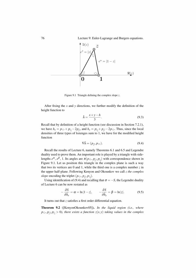
76 Lecture 9: Euler-Lagrange and Burgers equations.
<(z)
=(z)
0 1
z
eα = |1− z|
eβ = |z|
Figure 9.1 Triangle defining the complex slope z.
After fixing the x and y directions, we further modify the definition of theheight function to
h =x+ y−h
3. (9.3)
Recall that by definition of a height function (see discussion in Section 7.2.1),we have hx = p + p −2p , and hy = p + p −2p . Thus, since the localdensities of three types of lozenges sum to 1, we have for the modified heightfunction
∇h = (p , p ). (9.4)
Recall the results of Lecture 6, namely Theorems 6.1 and 6.5 and Legendreduality used to prove them. An important role is played by a triangle with side-lengths eα , eβ , 1. Its angles are π(p , p , p ) with correspondence shown inFigure 9.1. Let us position this triangle in the complex plane is such a waythat two its vertices are 0 and 1, while the third one is a complex number z inthe upper half-plane. Following Kenyon and Okounkov we call z the complexslope encoding the triplet (p , p , p ).
Using identification of (9.4) and recalling that σ =−S, the Legendre dualityof Lecture 6 can be now restated as
− ∂S∂ hx
= α = ln |1− z|, − ∂S∂ hy
= β = ln |z|. (9.5)
It turns out that z satisfies a first order differential equation.
Theorem 9.2 ([KenyonOkounkov05]). In the liquid region (i.e., wherep , p , p > 0), there exists a function z(x,y) taking values in the complex
77
upper half plane such that
(hx, hy) =1π(argz,−arg(1− z)) (9.6)
and−zx
1− z+
zy
z= 0. (9.7)
Proof It can be shown using general results on variational problems andPDEs that h is analytic in the liquid region — this is a particular caseof the Hilbert’s nineteenth problem, and we refer to the introduction of[DeSilvaSavin08] for references and discussion in the context of random sur-faces.
Then h is differentiable and (9.6) is a restatement of (9.4) and geometricdefinition of the complex slope z above.
By the Euler-Lagrange equations for the variational problem of Theorem5.15, we obtain using (9.5):
0 =∂
∂y
(∂S∂ hy
)+
∂
∂x
(∂S∂ hx
)=− ∂
∂yln |z|− ∂
∂xln |1− z|
Note that this is the real part of (9.7). For the imaginary part, we need to show
∂
∂yargz+
∂
∂xarg(1− z) = 0,
which is the identity hxy = hyx rewritten using (9.6).
We remark that the definition of the complex slope z is not canonical, sincewe need to somehow identify three angles of the (0,1,z) triangle with threeproportions (p , p , p ) and there are six ways to do it. In particular, if weperform the substitution u = z
1−z (this corresponds to a rearrangement of thevertices of the triangle of Figure 9.1), then the chain rule gives:
ux =zx
(1− z)2 , uy =zy
(1− z)2 .
In u–coordinate (9.7) becomes:
ux ·u = uy. (9.8)
This equation is well-known, it is called the complex inviscid Burgers equation.
Exercise 9.3. There are 6 ways to identify three angles of the (0,1,z) trianglewith three proportions (p , p , p ). Two of these ways lead to equations (9.7)and (9.8). Find the equations corresponding to four other ways.
78 Lecture 9: Euler-Lagrange and Burgers equations.
9.3 Generalization to qVolume–weighted tilings
We now consider a generalization of the uniformly random tilings by changingthe weight of the measure to a qVolume, where the volume is the number of unitcubes that must be added to the minimial tiling to obtain a given tiling.1 Addi-tion of one cube increases the height function h(x,y) of Section 1.4 by 3 at asingle point, hence, volume is given by the double integral 1
3
˜h(x,y)dxdy up
to a constant shift. In terms of the modified height function h of (9.3) additionof one cube decreases the height by 1 and, therefore, volume is equal to minusthe double integral: Volume =−
˜h(x,y)dxdy+ const.
Let us investigate the limit shape of the random height function under themeasure qVolume with q changing together with the linear size L of the domainby q = ec/L.
Proposition 9.4. Consider random tilings under the qVolume measure with q =
exp(c/L) as the linear size of the domain L grows. In the setting of Theorem5.15, the limit shape for the height function still exists in this case, it is givenby:
h∗ = argmaxh
¨R∗
(S(∇h)+
c3
h)
dxdy. (9.9)
Proof The proof is identical to the proof of the variational principle of The-orem 5.15 in the uniform case; we only need to multiply by qVolume when wecount tilings.
Corollary 9.5. The limit shape for qVolume–random lozenge tilings with q =
exp(c/L) satisfies:
div(∇S∇h) =c3
(9.10)
where is the evaluation operator; i.e., ∇S is being evaluated at ∇h and thendiv is applied to the resulting function of (x,y).
Proof This is the Euler-Lagrange equation for the variational problem (9.9).
Theorem 9.2 extends to the q–weighted case with a similar proof.
Corollary 9.6. For qVolume–weighted tilings with q = exp(c/L) the statementof Theorem 9.2 remains valid with (9.7) replaced by
−zx
1− z+
zy
z= c. (9.11)
1 The qVolume measure will appear again in Lectures 22-23 and then in Lecture 25. In particular,the effect of adding one cube on the height function is shown in Figure 25.2.
79
Proof The imaginary part of (9.11) is the same as that of (9.7) and its validityfollows from hxy = hyx relation. For the real part, we need to add an additionalterm in the Euler–Lagrange equations, which produces the right-hand side of(9.11). Note that c is being multiplied by (−3) when we pass from h to h by(9.3), hence, the final form of (9.11).
9.4 Complex characteristics method
Since (9.11) is a first order partial differential equation, it can be solved usingthe method of characteristics. The only tricky point is that the coordinate z iscomplex, while the textbooks usually present the method in the real case. Yet,as we will see in this and the next lecture, all the principles continue to workin the complex case.
For simplicity, imagine first that z were real. Consider any curvex(t),y(t),z(t) satisfying:
dxdt
(z−1) =dydt
z =dzdt· 1
cWe call such a curve a characteristic curve.
Proposition 9.7. A surface z = z(x,y) solving (9.11) must be a union of char-acteristic curves.
Proof The normal vector to such a surface is (zx,zy,−1). The tangent to acharacteristic curve is, up to scaling by a function of t, ( 1
z−1 ,1z ,c). Note that
these have dot product 0 by (9.11), so the tangent vector to the characteristiccurve is tangent to the surface. Thus, the characteristic curve remains on thesurface.
Next, we solve the equation determining the characteristic curves. Choosez = t. Then:
dydz
=1cz,
dxdz
=1
c(z−1).
The solutions to these equations are:
cy = lnz+ k1, cx = ln(z−1)+ k2.
Rearranging, we get the following form for a characteristic curve:
ze−cy = k1, (1− z)e−cx = k2,
where k1 and k2 are arbitrary constants. The choice of these constants is related
80 Lecture 9: Euler-Lagrange and Burgers equations.
to the specification of the boundary conditions for the PDE (9.11), so that weknow which curves to use to form the surface. In general a two-dimensionalsurface is a union of a one-parameter family of the curves, hence, we can pa-rameterize the desired k1, k2 by an equation Q(k1, k2) = 0. We conclude that thesolution to (9.11) must be given by Q(ze−cy,(1−z)e−cx) = 0 for some functionQ.
We proceed to the complex case and seek for a solution in the same form.The only difference is that Q is no longer arbitrary, but it is an analytic function.We have arrived at the following statement from [KenyonOkounkov05]:
Theorem 9.8. Let c 6= 0 and take any analytic function of two variablesQ(u,v). The surface given by:
Q(ze−cy,(1− z)e−cx) = 0 (9.12)
solves (9.11)
Proof Taking the derivatives in x and y of both sides of (9.12), we get
Q1zxe−cy +Q2(−zx)e−cx− cQ2(1− z)e−cx = 0,
Q1zye−cy− cQ2ze−cy +Q2(−zy)e−cx = 0,
where Qi denotes the derivative of Q in its i-th argument.Note that we can isolate Q1e−cy
Q2e−cx in both these expressions to obtain the equal-ity:
c(1− z)+ zx
zx=
zy
zy− cz
Clearing denominators and rearranging, we obtain precisely (9.11).
A remark is in order. The Burgers equation (9.11) is only valid in the liq-uid region. In the frozen part of the limit shape, only one type of lozengesis present and the definition of the complex slope z is meaningless. On theother hand, the limit shape is still analytic — it is in fact linear. However, non-analyticity appears on the Arctic boundary — separation curve between liquidand frozen phases; the behavior of the limit shape on two sides of this curve isvery different.
We still have not discussed how to find Q based on the boundary conditionsfor lozenge tilings. We examine this question in the next lecture.
Lecture 10: Explicit formulas for limitshapes
In the previous lectures we discussed two properties of the limit shapes oftilings: they solve a variational problem and in liquid regions they solve thecomplex Burgers equation. In this lecture we concentrate on algorithmic waysto explicitly identify the limit shapes.
10.1 Analytic solutions to the Burgers equation
First, we continue our study of the solutions to the complex Burgers equationappearing as Euler-Lagrange equation for limit shapes of random tilings. Theequation reads
−zx
1− z+
zy
z= c. (10.1)
In the last lecture we have shown in Theorem 9.8 that an analytic functionof two variables Q(u,v) gives rise to a solution to (10.1). However, we havenot explained whether every solution are obtained in this way, i.e. whether wecan use the formulation in terms of Q(u,v) as an ansatz for finding all possiblesolutions to the Burgers equation and, hence, for finding the limit shapes oftilings. We proceed by showing that this is indeed the case (still in the situationc 6= 0).
Theorem 10.1. If c 6= 0, given a solution to (10.1) there exists an analytic Qsuch that
Q(ze−cy,(1− z)e−cx) = 0.
Remark 10.2. In the present formulation Theorem 10.1 is a bit vague and weare not going to make it more precise here. Of course, one can always chooseQ to be identical zero, but this is not what we want. The theorem rather says
81
82 Lecture 10: Explicit formulas for limit shapes
that the first and second arguments of Q, ze−cy and (1− z)e−cx depend on eachother (locally near each point (x0,y0) of the liquid region) in an analytic way.The last property is easy to make precise in the case when the dependencies(x,y)→ ze−cy and (x,y)→ (1− z)e−cx are non-degenerate; this is what we doin the proof.
For the applications, the statement of Theorem 10.1 should be treated as anansatz: one should try to find a solution to (10.1) by searching for an analyticfunction Q. Often, Q will end up being very nice, like a polynomial in Theorem10.7 below.
If we knew the exact shape of the liquid region, then once Q is found, itautomatically provides the desired limit shape (maximizer) due to convexityof the functional in the variational problem of Theorem 5.15, which guaran-tees that a solution to the Euler-Lagrange equations is the global maximizer.However, the Euler–Lagrange equations or the complex Burgers equation donot tell anything about the behavior (extremality) in the frozen regions, andtherefore, additional checks are necessary there after Q is identified.
Sketch of the proof of Theorem 10.1 Take z(x,y) solving (10.1) and defineW = ze−cy and V = (1− z)e−cx. What we need to prove is that W (V ) is ananalytic function, in other words, W (V ) should satisfy the Cauchy-Riemannequations. This is equivalent to showing
∂W∂V
= 0.
Here we use the following notation: for a function f (z) : C→C with z = x+ iywe denote
∂ f∂ z
=12
(∂ f∂x− i
∂ f∂y
)and
∂ f∂ z
=12
(∂ f∂x
+ i∂ f∂y
).
The following lemma is the first step in computation.
Lemma 10.3. The Jacobian of the map (x,y)→ (V,W ) vanishes, i.e.
WxVy =VxWy.
Proof We have
WxVy = (zxe−cy)(−zye−cx)
and
VxWy = (−zxe−cx− c(1− z)e−cx)(zye−cy− cze−cy).
83
Therefore, subtracting and using (10.1) we find
VxWy−WxVy = e−cxe−cy(c2z(1− z)− czy(1− z)+ czxz) = 0,
as desired. The cancellation may seem (almost) magical; however the defini-tions of W and V were chosen by the method of characteristic essentially tohave this property.
Now consider W (V ) =W (V (x,y)) =W (x,y). Using the chain rule, we find
∂W∂x
=∂W∂V
(∂V∂x
)+
∂W∂V
(∂V∂x
)and
∂W∂y
=∂W∂V
(∂V∂y
)+
∂W∂V
(∂V∂y
).
Multiplying the first equation by ∂V∂y and subtracting the second equation mul-
tiplied by ∂V∂x , we get a restatement of Lemma 10.3:
0 =∂W∂x
∂V∂y− ∂W
∂y∂V∂x
=∂W∂V
(∂V∂x
∂V∂y− ∂V
∂y∂V∂x
).
This proves the desired Cauchy–Riemann relation ∂W∂V = 0 unless we have that(
∂V∂x
∂V∂y− ∂V
∂y∂V∂x
)= 0. (10.2)
The expression (10.2) coincides with the Jacobian of the transformation(x,y)→V from (two-dimensional) liquid region to complex numbers (anothertwo-dimensional real space) so as long as the mapping is not degenerate weare done. Note that in a similar manner we can demonstrate that ∂V
∂W = 0 givena similar non-degeneracy for the map (x,y)→W .
In other words, we have found Q(·, ·), which is analytic at any pairs of com-plex points (V (x,y),W (x,y)), where at least one of the maps (x,y)→ V (x,y),(x,y)→W (x,y) is non-degenerate. In a similar way, if we assume that (x,y)→αV (x,y)+βW (x,y) is non-degenerate near (x0,y0) for some numbers α andβ , then the possibility of choosing an analytic Q would also follow.
Theorems 9.8, 10.1 say that the map (x,y) 7→ (ze−y,(1− z)e−x) sends theliquid region to a one-dimensional complex Riemann surface in C2. In fact,this map is a bijection with its image, and therefore, it can be used to equip theliquid region with the structure of a one-dimensional complex manifold.
Lemma 10.4. In the liquid region, given (W,V ) = (ze−cy,(1−z)e−cx) one canrecover (x,y)
84 Lecture 10: Explicit formulas for limit shapes
Proof Note that given W,V one can immediately recover arguments of thecomplex numbers z and (1− z) as x,y are real. Given this, one can recoverz and since z 6= 0,1, as we are in the liquid region, we can therefore recoverx,y.
Next, we examine the c = 0 case.
Theorem 10.5. For a solution z(x,y) of the complex Burgers equation withc = 0 as in (9.7) there exists an analytic Q0 such that
Q0(z) = yz+ x(1− z). (10.3)
Remark 10.6. The discussion of Remark 10.2 also applies to Theorem 10.5.In addition, a solution z = const is possible for (9.7) with specific boundaryconditions. This corresponds to sending Q0 to infinity in (10.3), so that theright-hand side becomes irrelevant.
The arguments leading to Theorem 10.5 are similar to the c 6= 0 case and weomit all of this analysis except for the basic computation through the charac-teristics method.
The characterstic curves for−zx
1− z+
zy
z= 0
solvedxdt
(z−1) =dydt
(z)
and z is being kept constant. This gives dxdy = z
z−1 leading to the parameteriza-tion of the curves by two arbitrary constant k1, k2 via
x = yz
z−1+ k1, z = k2.
This is equivalent to x(1− z)+ yz = k1(1− k2) = Q0(z) of (10.3), where Q0
expresses the dependence between k1 and k2.
10.2 Algebraic solutions
Theorems 10.1 and 10.5 claim the existence of an abstract Q which describesthe liquid region. But how do we determine such Q? The following theorem ofKenyon and Okounkov shows that in the case of polygonal domains that Q isa polynomial.
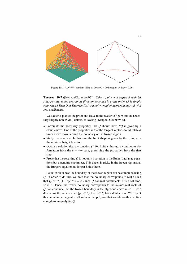
85
Figure 10.1 A qVolume–random tiling of 70×90×70 hexagon with q = 0.96.
Theorem 10.7 ([KenyonOkounkov05]). Take a polygonal region R with 3dsides parallel to the coordinate direction repeated in cyclic order. (R is simplyconnected.) Then Q in Theorem 10.1 is a polynomial of degree (at most) d withreal coefficients.
We sketch a plan of the proof and leave to the reader to figure out the neces-sary (highly non-trivial) details, following [KenyonOkounkov05].
• Formulate the necessary properties that Q should have. “Q is given by acloud curve”. One of the properties is that the tangent vector should rotate dtimes as we move around the boundary of the frozen region.
• Study c = −∞ case. In this case the limit shape is given by the tiling withthe minimal height function.
• Obtain a solution (i.e. the function Q) for finite c through a continuous de-formation from the c = −∞ case, preserving the properties from the firststep.
• Prove that the resulting Q is not only a solution to the Euler–Lagrange equa-tions but a genuine maximizer. This check is tricky in the frozen regions, asthe Burgers equation no longer holds there.
Let us explain how the boundary of the frozen region can be computed usingQ. In order to do this, we note that the boundary corresponds to real z suchthat Q(ze−cy,(1− z)e−cx) = 0. Since Q has real coefficients, z is a solution,so is z. Hence, the frozen boundary corresponds to the double real roots ofQ. We conclude that the frozen boundary is the algebraic curve in e−cx, e−cy
describing the values when Q(ze−cy,(1− z)e−cx) has a double root. We expectthis curve to be tangent to all sides of the polygon that we tile — this is oftenenough to uniquely fix Q.
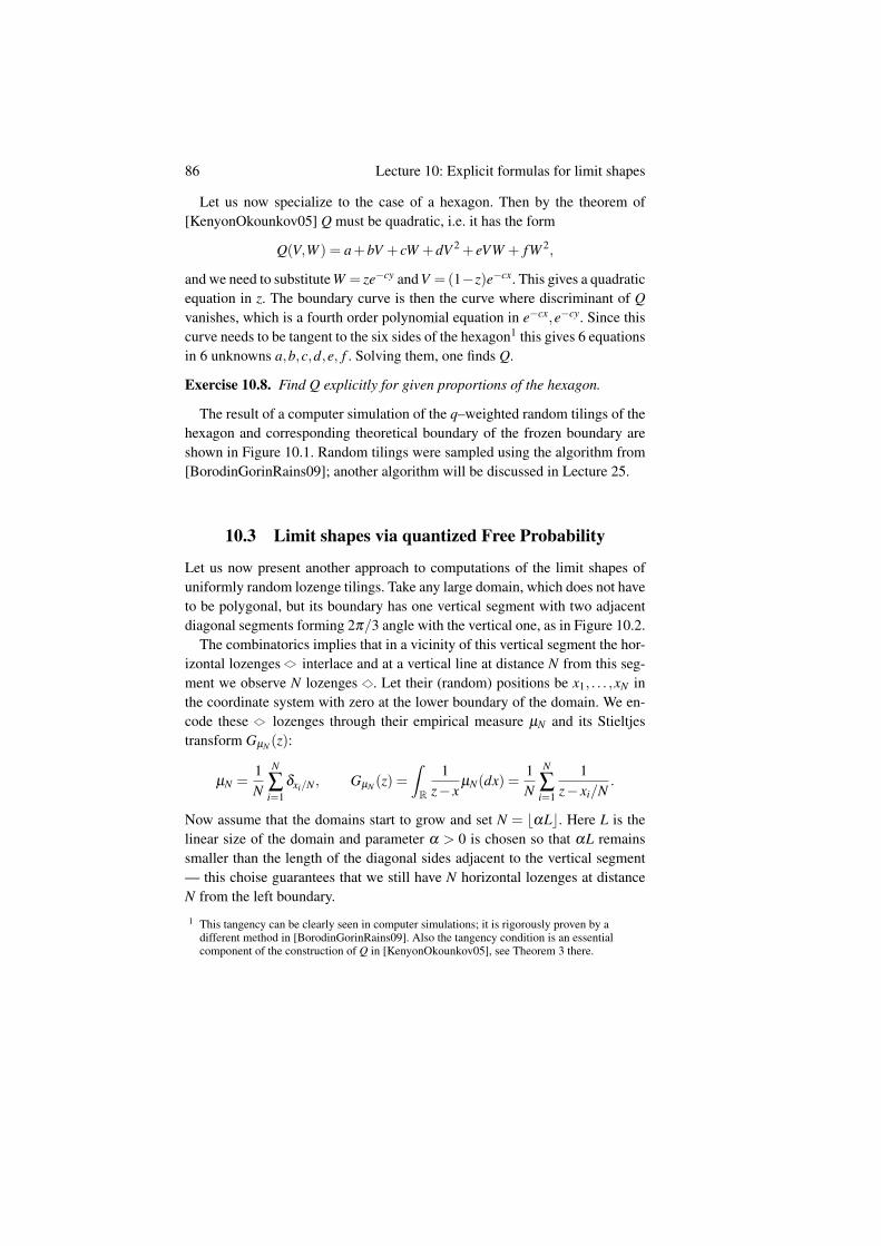
86 Lecture 10: Explicit formulas for limit shapes
Let us now specialize to the case of a hexagon. Then by the theorem of[KenyonOkounkov05] Q must be quadratic, i.e. it has the form
Q(V,W ) = a+bV + cW +dV 2 + eVW + fW 2,
and we need to substitute W = ze−cy and V =(1−z)e−cx. This gives a quadraticequation in z. The boundary curve is then the curve where discriminant of Qvanishes, which is a fourth order polynomial equation in e−cx,e−cy. Since thiscurve needs to be tangent to the six sides of the hexagon1 this gives 6 equationsin 6 unknowns a,b,c,d,e, f . Solving them, one finds Q.
Exercise 10.8. Find Q explicitly for given proportions of the hexagon.
The result of a computer simulation of the q–weighted random tilings of thehexagon and corresponding theoretical boundary of the frozen boundary areshown in Figure 10.1. Random tilings were sampled using the algorithm from[BorodinGorinRains09]; another algorithm will be discussed in Lecture 25.
10.3 Limit shapes via quantized Free Probability
Let us now present another approach to computations of the limit shapes ofuniformly random lozenge tilings. Take any large domain, which does not haveto be polygonal, but its boundary has one vertical segment with two adjacentdiagonal segments forming 2π/3 angle with the vertical one, as in Figure 10.2.
The combinatorics implies that in a vicinity of this vertical segment the hor-izontal lozenges interlace and at a vertical line at distance N from this seg-ment we observe N lozenges . Let their (random) positions be x1, . . . ,xN inthe coordinate system with zero at the lower boundary of the domain. We en-code these lozenges through their empirical measure µN and its Stieltjestransform GµN (z):
µN =1N
N
∑i=1
δxi/N , GµN (z) =ˆR
1z− x
µN(dx) =1N
N
∑i=1
1z− xi/N
.
Now assume that the domains start to grow and set N = bαLc. Here L is thelinear size of the domain and parameter α > 0 is chosen so that αL remainssmaller than the length of the diagonal sides adjacent to the vertical segment— this choise guarantees that we still have N horizontal lozenges at distanceN from the left boundary.
1 This tangency can be clearly seen in computer simulations; it is rigorously proven by adifferent method in [BorodinGorinRains09]. Also the tangency condition is an essentialcomponent of the construction of Q in [KenyonOkounkov05], see Theorem 3 there.
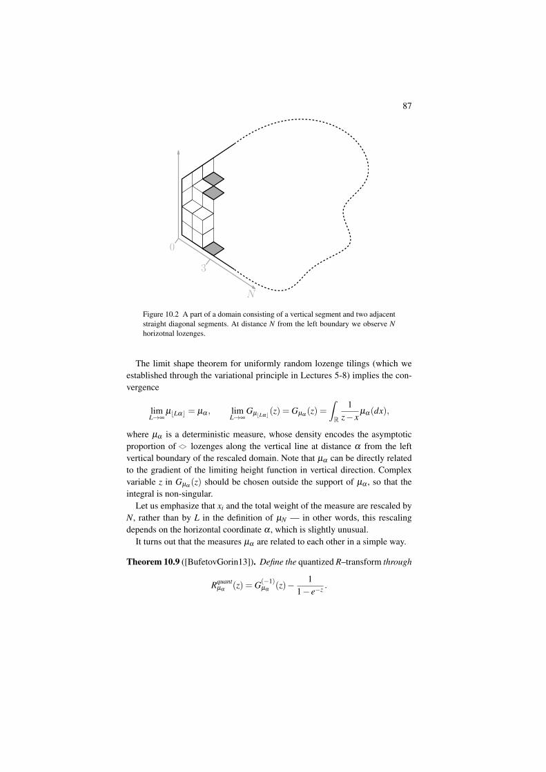
87
0
3
N
Figure 10.2 A part of a domain consisting of a vertical segment and two adjacentstraight diagonal segments. At distance N from the left boundary we observe Nhorizotnal lozenges.
The limit shape theorem for uniformly random lozenge tilings (which weestablished through the variational principle in Lectures 5-8) implies the con-vergence
limL→∞
µbLαc = µα , limL→∞
GµbLαc(z) = Gµα(z) =
ˆR
1z− x
µα(dx),
where µα is a deterministic measure, whose density encodes the asymptoticproportion of lozenges along the vertical line at distance α from the leftvertical boundary of the rescaled domain. Note that µα can be directly relatedto the gradient of the limiting height function in vertical direction. Complexvariable z in Gµα
(z) should be chosen outside the support of µα , so that theintegral is non-singular.
Let us emphasize that xi and the total weight of the measure are rescaled byN, rather than by L in the definition of µN — in other words, this rescalingdepends on the horizontal coordinate α , which is slightly unusual.
It turns out that the measures µα are related to each other in a simple way.
Theorem 10.9 ([BufetovGorin13]). Define the quantized R–transform through
Rquantµα
(z) = G(−1)µα
(z)− 11− e−z .
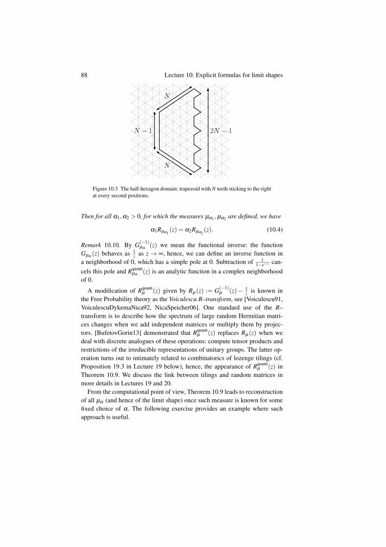
88 Lecture 10: Explicit formulas for limit shapes
N − 1
N
N
2N − 1
Figure 10.3 The half-hexagon domain: trapezoid with N teeth sticking to the rightat every second positions.
Then for all α1,α2 > 0, for which the measures µα1 ,µα2 are defined, we have
α1Rµα1(z) = α2Rµα2
(z). (10.4)
Remark 10.10. By G(−1)µα
(z) we mean the functional inverse: the functionGµα
(z) behaves as 1z as z→ ∞, hence, we can define an inverse function in
a neighborhood of 0, which has a simple pole at 0. Subtraction of 11−e−z can-
cels this pole and Rquantµα
(z) is an analytic function in a complex neighborhoodof 0.
A modification of Rquantµ (z) given by Rµ(z) := G(−1)
µ (z)− 1z is known in
the Free Probability theory as the Voiculescu R–transform, see [Voiculescu91,VoiculescuDykemaNica92, NicaSpeicher06]. One standard use of the R–transform is to describe how the spectrum of large random Hermitian matri-ces changes when we add independent matrices or multiply them by projec-tors. [BufetovGorin13] demonstrated that Rquant
µ (z) replaces Rµ(z) when wedeal with discrete analogues of these operations: compute tensor products andrestrictions of the irreducible representations of unitary groups. The latter op-eration turns out to intimately related to combinatorics of lozenge tilings (cf.Proposition 19.3 in Lecture 19 below), hence, the appearance of Rquant
µ (z) inTheorem 10.9. We discuss the link between tilings and random matrices inmore details in Lectures 19 and 20.
From the computational point of view, Theorem 10.9 leads to reconstructionof all µα (and hence of the limit shape) once such measure is known for somefixed choice of α . The following exercise provides an example where suchapproach is useful.
89
Exercise 10.11. Consider the domain of Figure 10.3, which is a trapezoidwith N teeth sticking out of the right boundary at every second positions. Bydefinition as N → ∞ the empirical measures on the right boundary convergeto µ1 which is a uniform measure on [0,2]. Use this observation together with(10.4) to compute the limit shape as N→ ∞.
In particular, Exercise 10.11 recovers the result of [NordenstamYoung11]which shows that the frozen boundary for this domain is a parabola.
The complex Burgers equation can be also extracted from the result of The-orem 10.9. The following exercise is close in spirit to the computations in[Gorin16, Section 4].
Exercise 10.12. Treating the formula (10.4) as a definition of the measures µα
(assuming one of them to be given) show that the limit shape of tilings encodedby these measures satisfies the complex Burgers equation (9.7).
Hint: The density of the measure µα can be reconstructed as the imagi-nary part of the Stieltjes transform Gµα
(z) as z approaches the real axis. Onthe other hand, in the definition of the Kenyon–Okounkov complex slope thedensity p becomes the argument of a certain complex number. This suggestreconstruction of complex slope by exponentiating the Stieltjes transform.
We end this lecture by a remark that in the random matrix theory to whichwe got linked through R–transforms, the complex Burgers equation has alsoshown up, see [Matytsin93, Guionnet02], which were even before the work of[KenyonOkounkov05].
Lecture 11: Global Gaussian fluctuationsfor the heights.
11.1 Kenyon-Okounkov conjecture
In previous lectures we found that the height function of random tilings for anarbitrary domain R converges in probability to a deterministic limit shape asthe size of the domain grows to infinity
1L
H(Lx,Ly) L→∞−−−→ h(x,y). (11.1)
The limit shape h(x,y) is a maximizer of a functional of the form¨R
S(∇h)dxdy, (11.2)
and can be also identified with solutions to the complex Burgers equation ona complex function z(x,y), where z encodes the gradient ∇h through a certaingeometric procedure.
In this section we start discussing the asymptotic fluctuations of the randomheight function around its expectation. The fluctuations are very different inthe liquid and frozen regions. In the latter, the height function is flat with over-helming probability already for finite values of L and hence, there are essen-tially no fluctuations. For the former, the situation is much more interesting.
Conjecture 11.1 ([KenyonOkounkov05], [Kenyon04]). Consider qVolume–weighted random tilings in domain R of linear size L and with q = exp(c/L).In the liquid region L ,
H(Lx,Ly)−E[H(Lx,Ly)] d−−−→L→∞
GFF, (11.3)
Where GFF is the Gaussian Free Field on L with respect to the complex struc-
90
91
ture given by ze−cy and with Dirichlet boundary conditions. The GFF is nor-malized, so that
Cov(H(Lx,Ly),H(Lx′,Ly′)
)≈− 1
2π2 lnd((x,y),(x′,y′)
)(11.4)
for (x,y) ≈ (x′,y′), with d(·, ·) denoting the distance in the local coordinatesgiven by the complex structure, and with normalization for the definition of theheight function as in (9.3), (9.4).
In this lecture we aim to define and understand the limiting object — theGaussian Free Field. The next lecture contains a heuristic argument towardsthe validity of Conjecture 11.1. Later on, in Lectures 22 and 23 we present aproof of a particular case of this conjecture for random plane partitions.
For general domains R, Conjecture 11.1 is a major open problem in thearea. Yet, there are several approaches to its proofs for particular classes ofdomains.
• One approach was suggested in [Kenyon99], [Kenyon00], [Kenyon04]. Thecorrelation functions of tilings are minors of the inverse Kasteleyn ma-trix, which can be thought of as a discrete harmonic function. On the otherhand, the covariance of GFF is a continuous harmonic function. Thus, onecan be treated as a discretization of another, which allows to use variousconvergence results from the analysis. Techically, two challenging pointsof such approach is to deal with non-trivial complex structure and withfrozen boundaries. Despite some progress (cf. [Russkikh16], [Russkikh18],[BerestyckiLaslierRay16]), the proofs along these lines until very recentlywere restricted to a special class of domains, which, in particular, have nofrozen regions. At the time of writing of this book new developments ap-peared in [ChelkakLaslierRusskikh20], [ChelkakRamassamy20]: the cen-tral idea is to construct a discrete approximation of the limiting complexstructure using the origami maps. There is a hope to reach a resolution ofConjecture 11.1 through this approach in the future.
• The second approach (see [BorodinFerrari08], [Petrov12b]) is to use a dou-ble contour integral representation for the inverse Kasteleyn matrix, and thenapply the steepest descent method for the asymptotic analysis. We will dis-cuss some components of this method in Lectures 14-16. This method isnaturally restricted to the domains, where such contour integral representa-tions are available. Yet, such domains include a class of specific polygonswith arbitrary many sides.
• The third approach combines a gadget called “Discrete Loop Equations”
92 Lecture 11: Global Gaussian fluctuations for the heights.
with the idea of applying differential/difference operators to inhomoge-neous partition functions to extract asymptotic information. We discuss dis-crete loop equations (cf. [BorodinGorinGuionnet15]) in Lecture 21 and theuse of difference operators for GFF asymptotics (cf. [BorodinGorin13],[BufetovGorin16], [Ahn18]) in Lectures 22-23. Tilings of non-simplyconnected domains with holes were analyzed through this approach in[BufetovGorin17].
• In some case, the marginal distributions of random tilings can be identifiedwith discrete log-gases, as we will compute in Lecture 19. Yet another ap-proach to global fluctuations exists in this case and links it to the asymptoticof recurrence coefficients of orthogonal polynomials, see [BreuerDuits13],[Duits15].
We remark that our toy example of the uniform measure on tilings of thehexagon is covered by each of the last three methods.
11.2 Gaussian Free Field
We start our discussion of Conjecture 11.1 by defining the (two-dimensional)Gaussian Free Field in a domain D ⊂ C in the standard complex structure ofC.
Take the laplace operator on D
4=∂
∂x2 +∂
∂y2
∣∣∣∣(x,y)∈D
.
We consider inverse operator −4−1 (note the minus sign) taken with Dirich-let (i.e., identical zero) boundary conditions on the boundary ∂D . 4−1 is anintegral operator (with respect to the Lebesgue measure on D), and its kernelis known as the Green’s function. Equivalently, we define:
Definition 11.2. The Green’s function GD (z,z′) on D with Dirichlet boundarycondition is a function G : D ×D → R of two complex arguments z = x+ iy,z′ = x′+ iy′, such that
4GD (z,z′) =−δ (z = z′),
where4 can be applied either in z or in z′ variables, and
GD (z,z′) = 0, if either z ∈ ∂D or z′ ∈ ∂D .
We remark without proof that for (non-pathological D) the Green’s func-tion exists, is unique and symmetric, i.e., GD (z,z′) = GD (z′,z). When D is
93
unbounded, one should add a logarithmic growth condition at ∞ to the defini-tion of the Green functions.
Exercise 11.3. Suppose that D is the upper halfplane H = z ∈ C | ℑz > 0.Show that in this case
GH(z,z′) =−1
2πln∣∣∣∣ z− z′
z− z′
∣∣∣∣. (11.5)
For general domains, there is often no explicit formula for the Green’s func-tion, but locally such function always grows like a logarithm of the distance:
GD (z,z′)∼− 12π
ln |z− z′| for z≈ z′. (11.6)
We can now present an informal definition of the Gaussian Free Field.
Definition 11.4. The Gaussian Free Field on D is a random Gaussian functionGFFD : D → R such that
E[GFFD
]= 0
E[GFFD (z)GFFD (z′)
]= GD (z,z′)
However, there is a problem with this definition, if z = z′, then GD (z,z′) =+∞, hence, the values of GFFD have infinite variance. This means that GFFD
is not a function, but a generalized function: we can not ask about the values ofthis random function at a point, but we can compute its integrals (or pairings)with reasonably smooth test functions.
Definition 11.5. For a test-function u : D → R, such that¨D
u(z)G(z,z′)u(z′)dxdydx′ dy′ < ∞, z = x+ iy, z′ = x′+ iy′,
we define a pairing of GFFD with u, as a mean zero Gaussian random variable〈GFFD ,u〉 with variance
E[〈GFFD ,u〉〈GFFD ,u〉
]=
¨D×D
u(z)G(z,z′)u(z′)dxdydx′ dy′.
If we take several such u’s, then the pairings are jointly Gaussian with covari-ance
E[〈GFFD ,u〉〈GFFD ,v〉
]=
¨D×D
u(z)G(z,z′)v(z′)dxdydx′ dy′. (11.7)
Informally, one should think about the pairings as integrals
〈GFFD ,u〉=¨
DGFFD (z, ·)u(z)dxdy. (11.8)
94 Lecture 11: Global Gaussian fluctuations for the heights.
From this point of view, one can take as u a (reasonably smooth) measure ratherthan a function.
By invoking the Kolmogorov consistency theorem, GFFD is well-defined asa stochastic process through Definition 11.5, if we show that the joint distri-butions appearing in this definition are consistent. Since they are all mean 0Gaussians, it suffices to check that the covariance is positive-definite.
Lemma 11.6. The covariance of 〈GFFD ,u〉 given by (11.7) is positive-definite.
Proof We need to check that the operator with kernel GD is positive-definite,which is equivalent to −4 being positive definite. The latter can be checkedintegrating by parts to reduce to the norm of the gradient:
〈−4u,u〉=¨
D
(−4u(z)
)u(z)dxdy =
¨D||∇u(z)||2L2 dxdy > 0.
Remark 11.7. A better alternative to Definition 11.5 would be to define a func-tional space (like the space of continuous functions in the definition of theBrownian motion) to which the GFFD belongs. We refer to [Sheffield03b],[Dubedat07, Section 4], [HuMillerPeres09, Section 2], [WernerPowell20] formore details on the definition of the Gaussian Free Field.
An important property of the Gaussian Free Field is its conformal invari-ance.
Recall that a map φ : D→D ′ is called conformal if it is holomorphic, bijec-tive and its inverse is also holomorphic. A direct computation with Laplacian4 leads to the conclusion that the Green’s function is preserved under confor-mal bijections, thus implying the following result:
Exercise 11.8. If φ is a conformal bijection of D with D ′, then
GFFD ′(φ(z))z∈D ′d= GFFD (z)z∈D .
For instance, in the case when the domain is upper half-plane, D =D ′ =H,the conformal bijections are Moebius transformations
z 7→ az+bcz+d
, a,b,c,d ∈ R,
and one readily checks that the formula (11.5) is unchanged under such trans-formations.
Another remark is that if we follow the same recipe for defining the GaussianFree Field in dimension 1, rather than 2, then we get the Brownian bridge.
Lemma 11.9. Consider the standard Brownian bridge,
B : [0,1]→ R , B(0) = B(1) = 0, (11.9)
95
which can be defined as the Brownian motion conditioned to be at 0 at time 1,or as a centered Gaussian process with covariance function
EBsBt = C (s, t) = min(t,s)(1−max(t,s)), 0≤ t,s≤ 1. (11.10)
Then the function C (s, t) is the kernel of the (minus) inverse Laplace operatoron the interval [0,1] with Dirichlet boundary conditions at 0 and 1.
Proof Since the Laplace operator in dimension 1 is simply the second deriva-tive, and the vanishing of C (s, t) at t = 0, s = 0, t = 1, and s = 1 is clear, itsuffices to check that
∂ 2
∂ t2 C (s, t) =−δ (s = t). (11.11)
We compute
∂C (s, t)∂ t
=
1− s , t < s
−s , t ≥ s.
Differentiating, we get (11.11).
We now give another informal definition of the Gaussian Free Field. Accord-ing to it, GFFD is a probability measure on functions f in D with 0 boundaryconditions with density
P( f )∼ exp(− 1
2
ˆD||∇ f ||2L2 dxdy
). (11.12)
The formula (11.12) is based on the well-known computation for the finite-dimensional Gaussian vectors:
Exercise 11.10. For a Gaussian vector v ∈ RN with probability density
f ∼√
detB√(2π)N
exp(−1
2〈v,Bv〉
),
the covariance matrix E[vvT ] is equal to B−1.
Since the covariance for the GFFD is given by the (minus) inverse Laplaceoperator, the matrix B appearing in its density should be identified with −4.Integrating by parts, we then arrive at the formula (11.12). We will repeatedlyuse (11.12) in the heuristic arguments of the following lectures. However, letus emphasize, that the precise mathematical meaning of (11.12) is very tricky:not only it is unclear with respect to which underlying measure the density iscomputed, but also the symbol ||∇ f ||2L2 is not well-defined for non-smooth f(and we already know that GFF is not smooth, even its values at points are notproperly defined).
96 Lecture 11: Global Gaussian fluctuations for the heights.
11.3 Gaussian Free Field in Complex Structures
The Gaussian Free Field appearing in Conjecture 11.1 is defined using thecomplex structure ze−cy rather than the standard complex structure of the plane.In this section we explain the meaning of this statement in two ways.
For the first approach, recall the results of Theorems 9.8, 10.1 and Lemma10.4. There exists an analytic function Q(v,w), such that the map
(x,y) 7→ (ze−cy,(1− z)e−cx) (11.13)
is a bijection of the liquid region L with (a part) of the curve Q(v,w) = 0 inC2. This part, being embedded in C2 has a natural local coordinate system onit; in particular, we can define the gradient and the Laplace operator on thecurve Q(v,w) = 0 and then use one of the definitions of GFF from the previoussection directly on this curve. Then we pullback the resulting field onto theliquid region L using the map (11.13). This is the desired field on Conjecture11.1.
For the second approach, given the liquid region L and complex slope z =z(x,y) on it we define the class of analytic functions. We give two closelyrelated definitions:
Definition 11.11. f : L → C is analytic with respect to ze−cy if for each(x0,y0) ∈L , there exists a holomorphic function g of complex variable, suchthat
f (x,y) = g(ze−cy) (11.14)
in a small neighborhood of (x0,y0).
Definition 11.12. f : L →C is analytic with respect to ze−cy if f satisfies thefirst order PDE:
fy
z− fx
1− z= 0 (11.15)
The complex Burgers equation of Corollary 9.6 implies that ze−cy itself sat-isfies (11.15): (
ze−cy)
y
z−(ze−cy
)x
1− z= 0. (11.16)
This can be used to show that (11.14) implies (11.15). If ze−cy is locally in-jective, then we can also argue in the opposite direction: (11.15) implies theCauchy–Riemann relations for the function g in (11.14) and two definitionsbecome equivalent.
All the above approaches accomplish the same goal: they create a structure
97
of a one-dimensional complex manifold (Riemann surface) on the liquid regionL . The general Riemann Uniformization Theorem says that all Riemann sur-faces of the same topology are conformally equivalent. In our case it specifiesto:
Theorem 11.13. There exists a conformal bijection Ω : L 7→ D with somedomain D ⊂ C, where D is equipped with the standard complex structure ofC, and the liquid region L is equipped with the complex structure of ze−cy,i.e., Ω is analytic by Definitions 11.11, 11.12.
In other words, Ω is an identification of (part of) the curve Q(v,w) = 0 ⊂C2 with a part of the plane C.
Definition 11.14. The Gaussian Free Field in the liquid region L is definedthrough
GFFL (x,y) = GFFD (Ω(x,y)).
This means, that for test functions u on L , its pairings with the Gaussian FreeField 〈GFFL ,u〉 are jointly Gaussian with covariance
E[〈GFFL ,u〉〈GFFL ,v〉
]=E
[〈GFFD , [uΩ
−1]·JΩ−1〉〈GFFD , [uΩ
−1]·JΩ−1〉
]=
ˆ ˆD×D
[uΩ−1](z)GD (z,z′)[vΩ
−1](z′)JΩ−1(z)JΩ−1(z′)dxdydx′ dy′,
(11.17)
where JΩ−1 is the Jacobian of the map Ω−1 and z = x+ iy, z′ = x′+ iy′.
Let us emphasize that under the map Ω, GFF is transformed as a function(rather than a distribution or measure); this again indicates that the test func-tions u should be treated as measures u(x+ iy)dxdy.
One might be worried that the map Ω in Theorem 11.13 is not unique, asit can be composed with any conformal bijection φ : D 7→ D ′. However, theconformal invariance of the Gaussian Free Field of Exercise 11.8 guaranteesthat the distribution of GFFL does not depend on the choice of Ω.
Finally, note that (11.4) differs from (11.6) by a factor of π . This is nota typo, but rather a universal constant appearing in tilings. We will see thisconstant appearing in the computation in the next section — the conceptualreasons for the particular value of the constant for random lozenge tilingsare not completely clear to us at this point. The same factor π appears in[KenyonOkounkovSheffield03, Theorem 4.5, see also Section 5.3.2] as a uni-versal normalization prefactor for random tilings with periodic weights.
Lecture 12: Heuristics for the Kenyon-Okounkov conjecture
This lecture focuses on a heuristic argument for the Kenyon-Okounkov con-jecture on the convergence of the centered height function to the GaussianFree Field. We concentrate only on the case c = 0, i.e., the uniform mea-sure, here. By the variational principle [CohnKenyonPropp00], in the limitmost height functions will be close to the unique maximizer h∗, which wehave pinned down (somewhat) explicitly in Lecture 9 by showing that the nor-malized shifted height function h∗ satisfies (h∗x, h∗y) =
1π(arg(z),−arg(1−z))
where z = z(x,y) satisfies the transformed Burgers equation
− zx
1− z+
zy
z= 0. (12.1)
The Kenyon-Okounkov conjecture focuses on the fluctuations about this limitshape and we repeat it now in the c = 0 case.
Conjecture 12.1 ([KenyonOkounkov05], [Kenyon04]). Take the same setupas in Theorem 5.15: let R∗ be a domain in R2 with piecewise-smooth boundary∂R∗ and a specified boundary height function hb. Take a sequence of domainsRL for a sequence L→∞, such that ∂RL
L → ∂R∗ and the boundary height func-tions converge as well. Now for each L consider the uniform probability mea-sure on tilings of RL. Finally, let H(Lx,Ly) be the value of the height functionof a random tiling of RL at (Lx,Ly). Then for the points (x,y)∈ R∗ in the liquidregion, as L→ ∞, the centered heights H(Lx,Ly)−E[H(Lx,Ly)] converge indistribution to the Gaussian free field in complex structure given by1 z.
Remark 12.2. Let us clarify the normalizations. If we choose the (modi-fied) definition of the height function as in (9.3), (9.4), then
√π(H(Lx,Ly)−
1 See previous lecture for a precise description of what this means.
98
99
E[H(Lx,Ly)]) should asymptotically behave as GFF of Definition 11.14 withshort-scale behavior of the covariance as in (11.6).
From here on, we will denote the liquid region by L . Recall from previouslectures that for large L, for a height function H on RL,
Pr(H)≈ exp(
L2¨
LS(∇H)dxdy
)(12.2)
(note that Pr(H) is really describing not a probability but a probability densityat H in the space of height functions, i.e. the probability of being close to H).
Since we would like to study limiting fluctuations about h∗, we can let H =
h∗+L−1g, where g is a random function supported in the liquid region whichrepresents the fluctuations about the limiting height function h∗. Plugging thisH into (12.2) yields
Pr(h∗+L−1g)≈ exp(
L2¨
LS(∇h∗+L−1
∇g)dxdy). (12.3)
We now Taylor expand the above integrand f (L−1) := S(∇h∗ + L−1∇g)with respect to the variable L−1, f (L−1) = f (0) + f ′(0)L−1 + 1
2 f ′′(0)L−2 +
(lower order terms). Using the chain rule, we have
f (0) = S(∇h∗),
f ′(0) = S1(∇h∗)gx +S2(∇h∗)gy,
where S1,S2 are the partial derivatives of S with respect to its first and secondcoordinate,viewing S as a function of two arguments h∗x ,h
∗y–the two coordi-
nates of ∇h∗. And
f ′′(0) = S11(∇h∗)(gx)2 +2S12(∇h∗)gxgy +S22(∇h∗)(gy)
2.
The first term yields an L-dependent normalizing constant exp(L2˜
L S(∇h∗))
which does not affect the probabilities. Because H = h∗ minimizes¨R∗
S(∇H)dxdy,
it follows thatddt
∣∣∣∣t=0
¨S(∇(h∗+ tg))dxdy = 0; (12.4)
this is exactly what was used to derive the Euler-Lagrange equations. Hence theintegral of the f ′(0)L−1 term vanishes. The L−2 in the quadratic term cancelswith the L2 outside the integral in (12.3), yielding a nonzero probability densityfunction at g.
100 Lecture 12: Heuristics for the Kenyon-Okounkov conjecture
Thus
Pr(h∗+L−1g)≈ exp(
L2¨
LS(∇h∗+L−1
∇g)dxdy)
= exp(
12
¨L
[S11(∇h∗)(gx)
2 +2S12(∇h∗)gxgy +S22(∇h∗)(gy)2]dxdy
)+ (lower order). (12.5)
Having completed this heuristic derivation, we can now (rigorously) show thatthe RHS of (12.5) is exactly what we would get if the height function fluctu-ations converged to a Gaussian free field. This is the content of the followinglemma.
Lemma 12.3. With the setup above, we have¨
L
[S11(∇h∗)(gx)
2 +2S12(∇h∗)gxgy +S22(∇h∗)(gy)2]dxdy
= 2πi¨
L
dgdz
dgdz
dz∧dz. (12.6)
Before proving this lemma, we show why when combined with (12.5) itshows that the fluctuations converge to a Gaussian free field. Recall from(11.12) in Lecture 11 that the Gaussian free field on a domain D may bethought of as a probability measure on functions on D which vanish on ∂D,with density
ρ( f )∼ exp(−1
2
¨D||∇ f ||2dxdy
). (12.7)
Since dz = dx+ idy and dz = dx− idy,
dz∧dz =−2idx∧dy. (12.8)
Similarly,
dgdz
=12
(∂g∂x− i
∂g∂y
), and
dgdz
=12
(∂g∂x
+ i∂g∂y
), (12.9)
so thatdgdz
dgdz
=14||∇g||2. (12.10)
Making these substitutions in Lemma 12.3 and combining with (12.5), we havethat the probability density on height function fluctuations g converges to theone in (12.7). This completes the heuristic argument for Gaussian free fieldfluctuations; the remainder of this lecture will be spent proving Lemma 12.3.
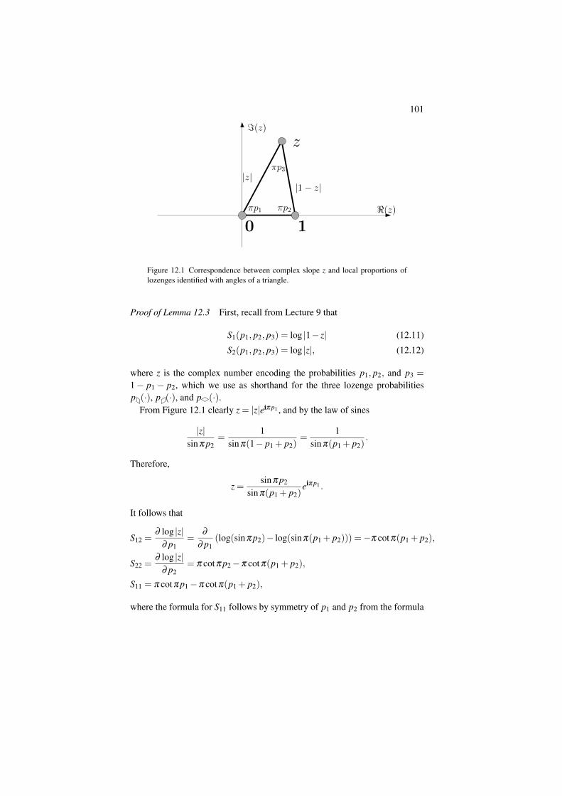
101
<(z)
=(z)
0 1
z
πp2
|1− z||z|
πp1
πp3
Figure 12.1 Correspondence between complex slope z and local proportions oflozenges identified with angles of a triangle.
Proof of Lemma 12.3 First, recall from Lecture 9 that
S1(p1, p2, p3) = log |1− z| (12.11)
S2(p1, p2, p3) = log |z|, (12.12)
where z is the complex number encoding the probabilities p1, p2, and p3 =
1− p1 − p2, which we use as shorthand for the three lozenge probabilitiesp (·), p (·), and p (·).
From Figure 12.1 clearly z = |z|eiπ p1 , and by the law of sines
|z|sinπ p2
=1
sinπ(1− p1 + p2)=
1sinπ(p1 + p2)
.
Therefore,
z =sinπ p2
sinπ(p1 + p2)eiπ p1 .
It follows that
S12 =∂ log |z|
∂ p1=
∂
∂ p1(log(sinπ p2)− log(sinπ(p1 + p2))) =−π cotπ(p1 + p2),
S22 =∂ log |z|
∂ p2= π cotπ p2−π cotπ(p1 + p2),
S11 = π cotπ p1−π cotπ(p1 + p2),
where the formula for S11 follows by symmetry of p1 and p2 from the formula
102 Lecture 12: Heuristics for the Kenyon-Okounkov conjecture
for S22.2 Recall that g is a function of x,y and also of (z, z), hence,
∂g∂x
=dgdz
zx +dgdz
zx, (12.13)
∂g∂y
=dgdz
zy +dgdz
zy. (12.14)
Therefore, combining the equations above, we have
S11(gx)2 +2S12gxgy +S22(gy)
2
= π
(− cotπ(p1 + p2)
(dgdz
(zx + zy)+dgdz
(zx + zy)
)2
+ cotπ p1
(dgdz
zx +dgdz
zx
)2
+ cotπ p2
(dgdz
zy +dgdz
zy
)2), (12.15)
which is a quadratic form in dgdz and dg
dz . We split our further calculation intothree claims.
Claim 12.4. The coefficient of(
dgdz
)2in (12.15) is 0.
Proof The coefficient is
π(−(zx + zy)2 cotπ(p1 + p2)+ z2
x cotπ p1 + z2y cotπ p2). (12.16)
Since zyz −
zx1−z = 0 by (12.1) we may write zx =
1−zz zy in the above, yielding
πz2y
(− 1
z2 cotπ(p1 + p2)+
(1− z
z
)2
cotπ p1 + cotπ p2
). (12.17)
Substituting
z =sinπ p2
sinπ(p1 + p2)eiπ p1 , 1− z =
sinπ p1
sinπ(p1 + p2)e−iπ p2 (12.18)
(the latter of which is easy to see by a similar law of sines argument on Figure12.1) to (12.17) yields
πz2y
z2 sin2π(p1 + p2)
(−cosπ(p1+ p2)sinπ(p1+ p2)+e−2πip2 cosπ p1 sinπ p1
+ e2πip1 cosπ p2 sinπ p2)
=πz2
y
2z2 sin2π(p1 + p2)
(−sin2π(p1+ p2)+e−2πip2 sin2π p1+e2πip1 sin2π p2).
2 Explicit formulas make is straightforward to show that det(
S11 S12S21 S22
)= π2, which actually
holds for the surface tensions in greater generality, see [KenyonOkounkov03, Section 2.2.3].
103
Splitting both complex exponentials into real and imaginary parts, the imagi-nary parts on the second and third of the above terms cancel, and the real partis
−sin2π(p1 + p2)+ sin2π p1 cos2π p2 + cos2π p1 sin2π p2 = 0
by the identity for sin(A+B). This proves the claim.
Claim 12.5. The coefficient of(
dgdz
)2in (12.15) is 0.
Proof The proof is exactly the same as for Claim 12.4.
Claim 12.6. The coefficient of dgdz
dgdz in (12.15), multiplied by dxdy as in the
integral in (12.6), is equal to dgdz
dgdz dz∧dz.
Proof First, since dz = zxdx+ zydy and dz = zxdx+ zydy,
dz∧dz = (zxzy− zxzy)dx∧dy =zyzy
zz(z− z)dx∧dy, (12.19)
where in the last step we use (12.1) to get
zxzy− zxzy = zyzy
(1− z
z− 1− z
z
)=
zyzy
zz(z− z).
Thus it suffices to show the following:
π(−cotπ(p1 + p2) ·2(zx + zy)(zx + zy)+ cotπ p1 ·2zxzx + cotπ p2 ·2zyzy)
?= 2πi
zyzy
zz(z− z). (12.20)
Again using zx =1−z
z zy to get a common factor of zyzy, and multiplying (12.20)by zz and dividing by 2πzyzy, we see (12.20) is equivalent to
i(z− z) ?=−cotπ(p1 + p2)+(1− z)(1− z)cotπ p1 + zzcotπ p2. (12.21)
Substituting (12.18), the LHS of (12.21) equals
2sinπ p1 sinπ p2
sinπ(p1 + p2)(12.22)
and the RHS equals
− cotπ(p1 + p2)+sin2
π p1
sin2π(p1 + p2)
cotπ p1 +sin2
π p2
sin2π(p1 + p2)
cotπ p2.
(12.23)
104 Lecture 12: Heuristics for the Kenyon-Okounkov conjecture
Multiplying through by sin2π(p1 + p2), we have that (12.20) is equivalent to
2sinπ(p1 + p2)sinπ p1 sinπ p2?=−cosπ(p1 + p2)sinπ(p1 + p2)
+ sinπ p1 cosπ p1 + sinπ p2 cosπ p2.
Moving all terms with sinπ(p1 + p2) to one side, this is the same as
sinπ(p1 + p2)(cosπ(p1 + p2)+2sinπ p1 sinπ p2)
?= sinπ p1 cosπ p1 + sinπ p2 cosπ p2.
Using the sine double angle identity and the formula cos(A+B), the desiredidentity becomes
sinπ(p1 + p2)(cosπ p1 cosπ p2− sinπ p1 sinπ p2 +2sinπ p1 sinπ p2)
?=
12
sin2π p1 +12
sin2π p2. (12.24)
Since
cosπ p1 cosπ p2− sinπ p1 sinπ p2 +2sinπ p1 sinπ p2
= cosπ p1 cosπ p2 + sinπ p1 sinπ p2 = cosπ(p1− p2),
(12.24) becomes
2sinπ(p1 + p2)cosπ(p1− p2)?= sin2π p1 + sin2π p2. (12.25)
This is true by simple trigonometry. We proved Claim 12.6 and hence Lemma12.3.
Exercise 12.7. Repeat the heuristic derivation of the GFF–fluctuations forgeneral c 6= 0, i.e. for the asymptotic of the qVolume–weighted lozenge tilings.
Remark 12.8. One expects that a similar computation (leading toGFF heuristics) can be done for dimers with periodic weights of[KenyonOkounkovSheffield03], however, this is not explicitly present in theliterature as of 2020. The arguments of [BorodinToninelli18, Section 3] mightturn out to be helpful for simplifying computations for such generalizations.
Remark 12.9. Can we turn the heuristics of this lecture into a rigorous proof ofconvergence of fluctuations to the GFF? This is very difficult and has not beendone. In particular, the very first step (12.2) had o(L2) error in the exponent,while we would need o(1) error for a rigorous proof.
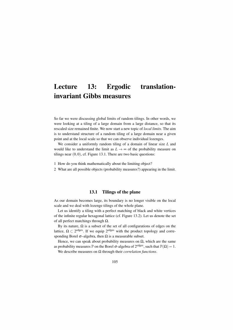
Lecture 13: Ergodic translation-invariant Gibbs measures
So far we were discussing global limits of random tilings. In other words, wewere looking at a tiling of a large domain from a large distance, so that itsrescaled size remained finite. We now start a new topic of local limits. The aimis to understand structure of a random tiling of a large domain near a givenpoint and at the local scale so that we can observe individual lozenges.
We consider a uniformly random tiling of a domain of linear size L andwould like to understand the limit as L→ ∞ of the probability measure ontilings near (0,0), cf. Figure 13.1. There are two basic questions:
1 How do you think mathematically about the limiting object?2 What are all possible objects (probability measures?) appearing in the limit.
13.1 Tilings of the plane
As our domain becomes large, its boundary is no longer visible on the localscale and we deal with lozenge tilings of the whole plane.
Let us identify a tiling with a perfect matching of black and white verticesof the infinite regular hexagonal lattice (cf. Figure 13.2). Let us denote the setof all perfect matchings through Ω.
By its nature, Ω is a subset of the set of all configurations of edges on thelattice, Ω ⊂ 2edges. If we equip 2edges with the product topology and corre-sponding Borel σ–algebra, then Ω is a measurable subset.
Hence, we can speak about probability measures on Ω, which are the sameas probability measures P on the Borel σ -algebra of 2edges, such that P(Ω) = 1.
We describe measures on Ω through their correlation functions.
105
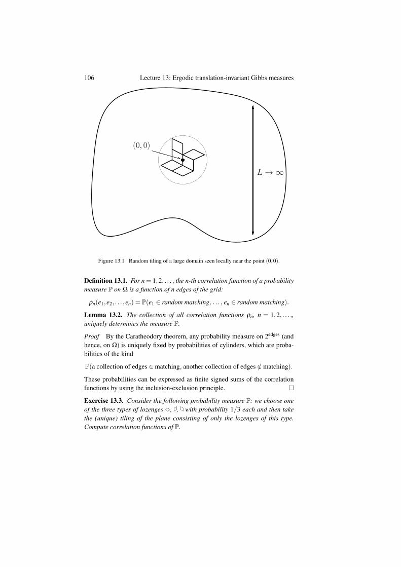
106 Lecture 13: Ergodic translation-invariant Gibbs measures
(0, 0)
L → ∞
Figure 13.1 Random tiling of a large domain seen locally near the point (0,0).
Definition 13.1. For n = 1,2, . . . , the n-th correlation function of a probabilitymeasure P on Ω is a function of n edges of the grid:
ρn(e1,e2, . . . ,en) = P(e1 ∈ random matching, . . . , en ∈ random matching).
Lemma 13.2. The collection of all correlation functions ρn, n = 1,2, . . . ,,uniquely determines the measure P.
Proof By the Caratheodory theorem, any probability measure on 2edges (andhence, on Ω) is uniquely fixed by probabilities of cylinders, which are proba-bilities of the kind
P(a collection of edges ∈matching, another collection of edges /∈matching).
These probabilities can be expressed as finite signed sums of the correlationfunctions by using the inclusion-exclusion principle.
Exercise 13.3. Consider the following probability measure P: we choose oneof the three types of lozenges , , with probability 1/3 each and then takethe (unique) tiling of the plane consisting of only the lozenges of this type.Compute correlation functions of P.
107
Figure 13.2 Infinite regular hexagonal graph.
13.2 Properties of the local limits
When a measure P on Ω appears as a local limit of uniform measures on tilingsof planar domains, it is not an arbitrary measure. Let us list the main propertiesthat we expect such measure to have.
Definition 13.4. A measure P on Ω is called Gibbs, if for any finite subdomainR (=collection of vertices), the conditional measure on perfect matching of Rgiven that all vertices of R are matched with vertices of R, but not outside (andin addition one can condition on any event outside R), is the uniform measure.
The Gibbs property is a way to say that a measure is uniform for the situationwhen the state space Ω is infinite. Clearly, uniform measure on tilings of anyfinite domain is Gibbs, as the conditionings do not change uniformity. Hence,we expect every local limit of tilings also to be Gibbs.
Definition 13.5. A measure P on Ω is called translationally invariant, if thecorrelation functions are unchanged upon translations of all arguments by asame vector.
Why do we expect local limits to be translationally invariant? This propertyshould be treated as some kind of a continuity statement. In general, the locallimit might depend on the macroscopic zoom-in position inside the domain.However, if we believe that this dependence is continuous, then a shift by afinite vector should become negligible in the large domain limit, and, hence,should not change the local limit.
108 Lecture 13: Ergodic translation-invariant Gibbs measures
Let us take two Gibbs translationally invariant measures µ1 and µ2. Forevery 0 < α < 1 the (convex) linear combination αµ1 +(1−α)µ2 is also aGibbs translationally invariant measure. Hence, such measures form a convexset.
Definition 13.6. A Gibbs translationally invariant measure is called ergodic,if it is an extreme point of the set of all such measures, i.e. if it can not bedecomposed into convex linear combination of two distinct measures from thisclass.
We abbreviate EGTI for ergodic Gibbs translationally invariant measures.
Lemma 13.7. If P is an EGTI probability measure, and A is a translationallyinvariant event, then either P(A) = 0 or P(A) = 1.
Remark 13.8. By definition, a translationally invariant event in Ω is a subsetof Ω, which is preserved under shifts of the entire grid. For example, if Rn isa growing sequence of convex domains (say, rectangles) exhausting the plane,then
limsupn→∞
number of horizontal edges of matching inside Rn
area of Rn≤ 1
7
is a translationally invariant event.
Proof of Lemma 13.7 We argue by contradiction. Assume that 0 < P(A)< 1and let A be the complementary event. Define P1 to be the normalized restric-tion of P onto the set A, i.e.,
P1(B) =P(A∩B)P(A)
.
Also define P2 to be the normalized restriction of P onto the set A, i.e.,
P2(B) =P(A∩B)P(A)
.
Then both P1 and P2 are Gibbs translationally invariant measures and
P(·) = P(A)P1(·)+P(A)P2(·).
Therefore, P is not ergodic.
Exercise 13.9. Show that the measure P of Exercise 13.3 is Gibbs and transla-tionally invariant, but not ergodic. Represent it is as a convex linear combon-ation of EGTI measures.
109
13.3 Slope of EGTI measure
Let us introduce an important numeric characteristic of an EGTI measure.
Definition 13.10. Slope of an EGTI probability measure on Ω is a triplet(p , p , p ) of non-negative numbers summing up to 1, defined in either oftwo equivalent ways:
1 For an arbitrary triangle of the grid (=vertex of the hexagonal lattice), p ,p , p are probabilities that this trangle belows to a lozenge of a corre-sponding type (is matched to one of the three corresponding adjacent ver-tices of another color).
2 If Rn is a growing sequence of convex domains (say, rectangles) exhaustingthe plane, then
p = limn→∞
number of triangles inside Rn covered by lozenges of typenumber of triangles inside Rn
,
(13.1)and similarly for p and p .
Remark 13.11. The probabilities in the first definition of the slope do not de-pend on the choice of the triangle due to the translation invariance of the mea-sure.
The limits in (13.1) exist almost surely, which is a property that needs tobe proven. (If we know that the limits exist, they have to be deterministic dueto ergodicity.) One way to prove that the limits in (13.1) exist in probability(rather than the stronger condition of being almost sure limits) is by boundingthe variance of the right-hand side, using the explicit description of the EGTImeasures given later in this lecture.
As soon as we know that a deterministic limit in (13.1) exists, it has to beequal to p from the first definition, as this is the expectation of the right-handside in (13.1).
The possible slopes (p , p , p ) form a triangle: p > 0, p > 0, p > 0,p + p + p = 1. We say that the slope is extreme, if one of the proportionsof lozenges, p , p , or p is zero, and non-extreme otherwise.
Theorem 13.12 ([Sheffield03a]). For each non-extreme slope there exists aunique EGTI probability measure of such slope.
Idea of the proof. Suppose that there are two different EGTI measures of thesame slope and let π1, π2 be corresponding random perfect matchings fromΩ sampled independently. Superimpose π1 and π2, i.e. consider the union ofall edges of the hexagonal lattice appearing in either of the matchings. Then
110 Lecture 13: Ergodic translation-invariant Gibbs measures
π1 ∪π2 is a collection of double edges (if the same edge belonged to both π1
and π2), finite cycles (of alternating edges from π1 and π2), and infinite curvesextending to infinity (again of alternating edges from π1 and π2).
Claim. Almost surely, π1 ∪ π2 has double edges and finite cycles, but noinfinite curves.
The claim is a difficult statement and we refer to [Sheffield03a] for the proof.Note that for measures of different slopes it no longer holds.
Given the claim, let us show that the distributions of π1 and π2 coincide.For that we demonstrate a sampling procedure, which is the same for bothmeasures.
Note that given a cycle of π1∪π2, half of its edges belong to π1 and anotherhalf belongs to π2. There are two options: either all even edges belong to π1
(and all odd edges belong to π2) or all even edges belong to π2. ApplyingGibbs property to this cycle separately for π1 and for π2, we see that thesetwo options arise with equal probability 1
2 . Hence, we can sample π1 by thefollowing procedure: first sample π1 ∪ π2, and then flip an independent coinfor each cycle to decide which of its edges belong to π1. Since the procedurefor π2 is the same, we are done.
Theorem 13.12 has an interesting corollary. First, it explains why we ex-pect local limits of random tilings to be ergodic: indeed, we want them to havefixed slopes matching the slope of the global macroscopic limit shape. Thisargument can be also reversed: if we knew a priory that the local limits of ran-dom tilings should be given by ergodic Gibbs translation invariant measures,then Theorem 13.12 would uniquely fix such measure. Unfortunately, in prac-tice, checking the EGTI property is hard, with, perhaps, the most complicatedpart being translation invariance.
Nevertheless, it was conjectured in [CohnKenyonPropp00, Conjecture 13.5]that all the limits are EGTI, which was recently proven in [Aggarwal19].
Theorem 13.13 ([Aggarwal19]). Locally, near any point of a (proportionallygrowing) domain with non-extreme slope of the limit shape, the uniform mea-sure on tilings converges to EGTI measure of the same slope.
In Lecture 17 we present a partial result in the direction of Theorem 13.13from [Gorin16] after some preparations in Lectures 14, 15, and 16. The proofof the general case in [Aggarwal19] starts with the same approach and thenadds to it several additional ideas which we are not going to present in theselectures.
111
13.4 Correlation functions of EGTI measures
Theorem 13.13 provides a simple way to identify the EGTI measures for eachslope. We need to take any domain where such slope appears and compute thelocal limit. In fact, we already made such computation when analyzing tilingson the torus in Lecture 4 and the result is given by Theorem 4.11 there. Let usrecast the result here.
Corollary 13.14. For an EGTI measure of slope (p , p , p ), the nth
correlation function computing the probability of observing the edges(x1,y1, x1, y1), . . . ,(xn,yn, xn, yn) between white vertices (xi,yi) and black ver-tices (xi, yi) in a random perfect matching is
ρn((x1,y1, x1, y1), . . . ,(xn,yn, xn, yn))
=n
∏i=1
K00(xi,yi, xi, yi) det1≤i, j,≤n
(Kα,β [xi− x j, yi− y j]) (13.2)
where
Kα,β (x,y) ="|z|=|w|=1
wxz−y
1+ eα z+ eβ wdw
2πiwdz
2πiz,
we use the coordinate system of Figure 3.2, K00(xi,yi, xi, yi) are weights fromthat figure, and the correspondence between (p , p , p ) and (α,β ) is as inTheorem 6.1.
Remark 13.15. At this point the Gibbs property of the measure might seemto be very far away from the determinantal formulas for the correlation func-tions. However, the Gibbsianity can actually be directly seen from (13.2), asexplained in [BorodinShlosman08].
Let us get comfortable with formula (13.2) by computing the correlationfunctions of horizontal lozenges along a vertical line. This corresponds totaking xi = 1, xi = 0 and yi = yi. Hence, absorbing the K0,0 prefactor (which iseβ in this case) into the determinant, we conclude that the correlation functionsof horizontal lozenges at positions yi are minors of the matrix
"|z|=|w|=1
eβ wzy
1+ eα z+ eβ wdw
2πiwdz
2πiz, (13.3)
We further compute the w–integral as a residue at the unique pole of the inte-grand to get
12πi
ˆ z0
z0
zy−1dz =zy
0− zy0
2πiy=|z0|y
πysin(Arg(z0)y).
112 Lecture 13: Ergodic translation-invariant Gibbs measures
Note that the |z0|y prefactor cancels out when we compute the minors. Bylooking at y = 0 case, we also match Arg(z0) with π p . Hence, we reach aconclusion.
Corollary 13.16. For the EGTI probability measure of slope (p , p , p )
P( at positions (0,y1), . . . ,(0,yn)) = det[K(yi− y j)]ni, j=1,
with
K(y) =
sin(π p y)
πy, y 6= 0,
p , y = 0.(13.4)
Remark 13.17. Rotating by 120 degrees, we can also get similar statements forthe and lozenges — their distributions along appropriate sections will bedescribed by (13.4) with parameter p replaced by p and p , respectively.
Exercise 13.18. Perform the computation of Remark 13.17 in details.
The kernel of (13.4) has the name discrete sine kernel and the point processof Corollary 13.16 is called the discrete sine process.
The continuous counterpart of the sine process (when y’s become real num-bers rather than integers) is a universal object in the random matrix theory1,where it describes local limits for the eigenvalues in the bulk of the spectrumof large complex Hermitian matrices, see [Kuijlaars11, TaoVu12, Lubinsky16,ErdosYau17] for recent reviews. Conjecturally, sine process also appears inmany other settings such as large eigenvalues of Laplace operator in variousdomains or even spacings between zeros of Riemann zeta-function.
13.5 Frozen, liquid, and gas phases
An important property of the EGTI measure with non-degenerate slope(p , p , p ) satisfying p , p , p > 0 is the polynomial decay of the correla-tions between lozenges with distance. This can be directly seen from the resultof Corollary 13.14, since Kα,β (x,y) decays polynomially in x and y. This typeof EGTI measures is called the liquid phase in [KenyonOkounkovSheffield03]with an alternative name being the rough unfrozen phase.
Extreme slopes (when either p , or p , or p vanishes) lead to very differentstructure of the EGTI measure: the random tiling becomes degenerate and hasnon-decaying correlations. This is the frozen phase.
1 We return to the connection between tilings and random matrix theory in Lectures 19 and 20.
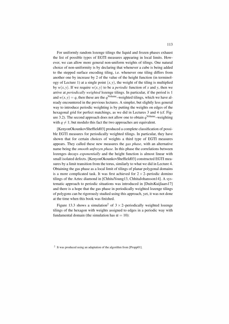
113
For uniformly random lozenge tilings the liquid and frozen phases exhaustthe list of possible types of EGTI measures appearing in local limits. How-ever, we can allow more general non-uniform weights of tilings. One naturalchoice of non-uniformity is by declaring that whenever a cube is being addedto the stepped surface encoding tiling, i.e. whenever one tiling differs fromanother one by increase by 2 of the value of the height function (in terminol-ogy of Lecture 1) at a single point (x,y), the weight of the tiling is multipliedby w(x,y). If we require w(x,y) to be a periodic function of x and y, then wearrive at periodically weighted lozenge tilings. In particular, if the period is 1and w(x,y) = q, then these are the qVolume–weighted tilings, which we have al-ready encountered in the previous lectures. A simpler, but slightly less generalway to introduce periodic weighting is by putting the weights on edges of thehexagonal grid for perfect matchings, as we did in Lectures 3 and 4 (cf. Fig-ure 3.2). The second approach does not allow one to obtain qVolume–weightingwith q 6= 1; but modulo this fact the two approaches are equivalent.
[KenyonOkounkovSheffield03] produced a complete classification of possi-ble EGTI measures for periodically weighted tilings. In particular, they haveshown that for certain choices of weights a third type of EGTI measuresappears. They called these new measures the gas phase, with an alternativename being the smooth unfrozen phase. In this phase the correlations betweenlozenges decays exponentially and the height function is almost linear withsmall isolated defects. [KenyonOkounkovSheffield03] constructed EGTI mea-sures by a limit transition from the torus, similarly to what we did in Lecture 4.Obtaining the gas phase as a local limit of tilings of planar polygonal domainsis a more complicated task. It was first achieved for 2× 2–periodic dominotilings of the Aztec diamond in [ChhitaYoung13, ChhitaJohansson14]. A sys-tematic approach to periodic situations was introduced in [DuitsKuijlaars17]and there is a hope that the gas phase in periodically weighted lozenge tilingsof polygons can be rigorously studied using this approach, yet, it was not doneat the time when this book was finished.
Figure 13.3 shows a simulation2 of 3× 2–periodically weighted lozengetilings of the hexagon with weights assigned to edges in a periodic way withfundamental domain (the simulation has α = 10):
2 It was produced using an adaptation of the algorithm from [Propp01].
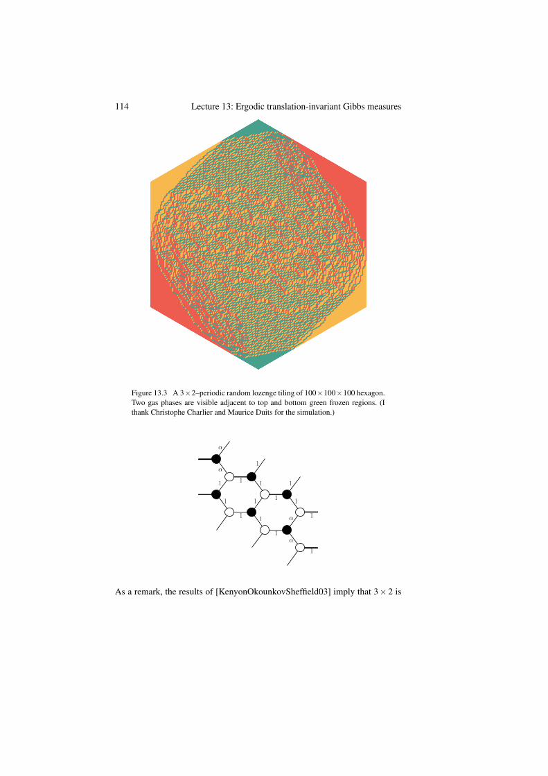
114 Lecture 13: Ergodic translation-invariant Gibbs measures
Figure 13.3 A 3×2–periodic random lozenge tiling of 100×100×100 hexagon.Two gas phases are visible adjacent to top and bottom green frozen regions. (Ithank Christophe Charlier and Maurice Duits for the simulation.)
1
1
1
1
1
1
1
1
1
1
1
α
α
α
α
1
1
1
As a remark, the results of [KenyonOkounkovSheffield03] imply that 3×2 is
115
the minimal size of the fundamental domain, which makes the appearance of agas phase possible.
The phenomenology for periodically weighted tilings becomes richerthan for the uniform case, which we mostly study in this book andwe refer to [Mktchyan19], [CharlierDuitsKuijlaarsLennels19], [Charlier20],[BeffaraChhitaJohansson20] for some results. Just as an example, while for theuniformly random lozenge tilings we could observe only three frozen phasescorresponding to 3 types of lozenges, for 2× 2 periodic case another frozenphase is possible, in which densities of two types of lozenges are equal to 1/2and the corresponding stepped surface looks like a staircase.
Lecture 14: Inverse Kasteleyn matrix fortrapezoids.
Our goal over the next few lectures is to discuss a local limit theorem for thetrapezoid (or sawtooth) domain of Figure 14.1. It is so named because of the“dents” along its right edge. We are going to prove that local structure of uni-formly random lozenge tilings for such domains is asymptotically governed byergordic translationally invariant Gibbs measures introduced in the last lecture.
Why should we study this particular class of domains?
• The sawtooth domains are integrable in the sense that they have explicitinverse Kasteleyn matrix;
• This type of domains has links to representation theory. In particular, con-sider a sawtooth domain with width N and dents at locations t1 > · · · > tN .Writing λ j = t j− (N− j), we see that λ1 ≥ ·· · ≥ λN . Each representationsof the unitary group U(N) has a signature , and it turns out that the numberof tilings of the sawtooth domain is given by the (vector space) dimensionof the representations having signature (λ1, . . . ,λN), and by the Weyl di-mension formula this is given by ∏i< j
(λi−i)−(λ j− j)j−i . We come back to this
computation in Lecture 19, see Proposition 19.3.
• The boundary of every domain locally looks like a trapezoid; eventually,the results for sawtooth domains and their extensions can be used as abuilding block for proving the local limit theorem for general domains, see[Aggarwal19] and [Gorin16].
In Lecture 3 (see Theorem 3.5) we expressed the correlation functions of ran-dom tilings through the inverse Kasteleyn matrix. The goal of this lecture isto compute this inverse matrix explicitly, which will be the main tool for ouranalysis in the subsequent lecture.
Following the notations of [Petrov12a] (which this lecture is based on), we
116
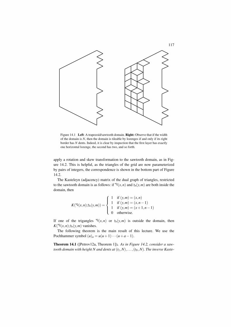
117
Figure 14.1 Left: A trapezoid/sawtooth domain. Right: Observe that if the widthof the domain is N, then the domain is tileable by lozenges if and only if its rightborder has N dents. Indeed, it is clear by inspection that the first layer has exactlyone horizontal lozenge, the second has two, and so forth.
apply a rotation and skew transformation to the sawtooth domain, as in Fig-ure 14.2. This is helpful, as the triangles of the grid are now parameterizedby pairs of integers, the correspondence is shown in the bottom part of Figure14.2.
The Kasteleyn (adjacency) matrix of the dual graph of triangles, restrictedto the sawtooth domain is as follows: if (x,n) and (y,m) are both inside thedomain, then
K( (x,n); (y,m)) =
1 if (y,m) = (x,n)1 if (y,m) = (x,n−1)1 if (y,m) = (x+1,n−1)0 otherwise.
If one of the trigangles (x,n) or (y,m) is outside the domain, thenK( (x,n); (y,m) vanishes.
The following theorem is the main result of this lecture. We use thePochhammer symbol (u)a = u(u+1) · · ·(u+a−1).
Theorem 14.1 ([Petrov12a, Theorem 1]). As in Figure 14.2, consider a saw-tooth domain with height N and dents at (t1,N), . . . ,(tN ,N). The inverse Kaste-
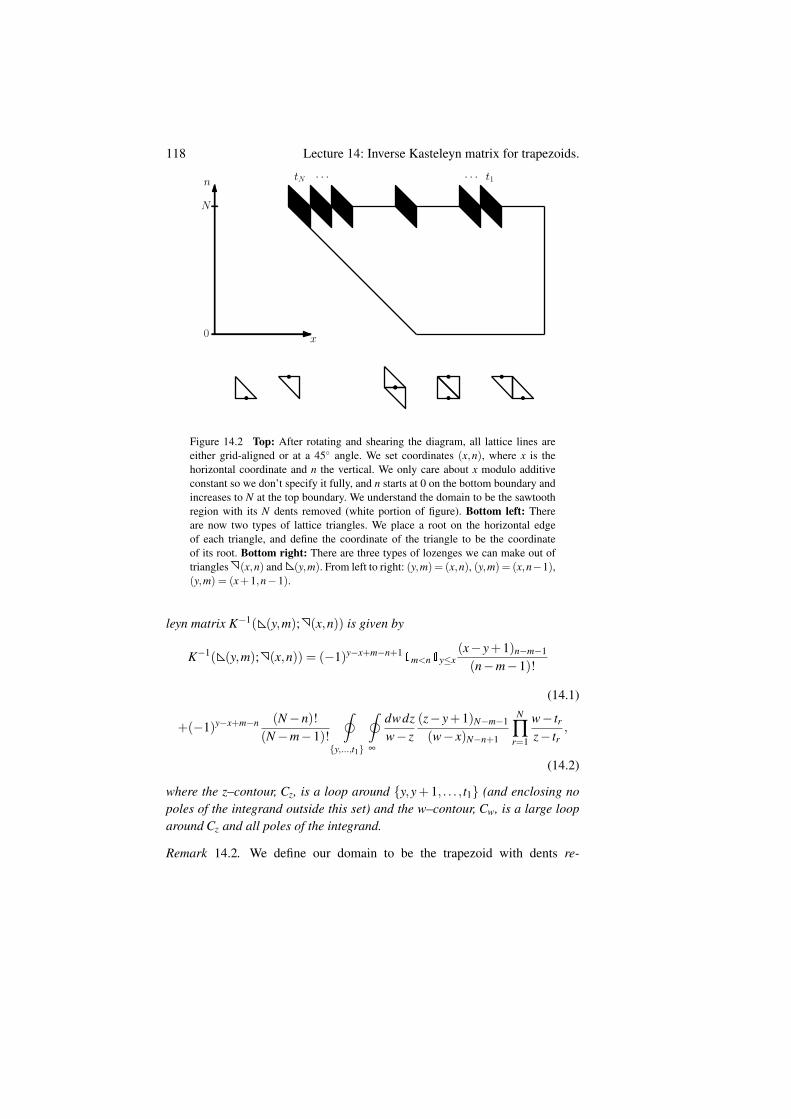
118 Lecture 14: Inverse Kasteleyn matrix for trapezoids.
n
N
0 x
tN · · · · · · t1
Figure 14.2 Top: After rotating and shearing the diagram, all lattice lines areeither grid-aligned or at a 45 angle. We set coordinates (x,n), where x is thehorizontal coordinate and n the vertical. We only care about x modulo additiveconstant so we don’t specify it fully, and n starts at 0 on the bottom boundary andincreases to N at the top boundary. We understand the domain to be the sawtoothregion with its N dents removed (white portion of figure). Bottom left: Thereare now two types of lattice triangles. We place a root on the horizontal edgeof each triangle, and define the coordinate of the triangle to be the coordinateof its root. Bottom right: There are three types of lozenges we can make out oftriangles (x,n) and (y,m). From left to right: (y,m) = (x,n), (y,m) = (x,n−1),(y,m) = (x+1,n−1).
leyn matrix K−1( (y,m); (x,n)) is given by
K−1( (y,m); (x,n)) = (−1)y−x+m−n+11m<n1y≤x
(x− y+1)n−m−1
(n−m−1)!
(14.1)
+(−1)y−x+m−n (N−n)!(N−m−1)!
˛
y,...,t1
˛
∞
dwdzw− z
(z− y+1)N−m−1
(w− x)N−n+1
N
∏r=1
w− trz− tr
,
(14.2)
where the z–contour, Cz, is a loop around y,y+ 1, . . . , t1 (and enclosing nopoles of the integrand outside this set) and the w–contour, Cw, is a large looparound Cz and all poles of the integrand.
Remark 14.2. We define our domain to be the trapezoid with dents re-
119
moved, and therefore, the above formula is applicable only for triangles(y,m), (x,n) which lie entirely in the white region of Figure 14.2 (Top).
In particular, we do not allow (x,n) ∈ (t1,N), . . . , (tN ,N) as these cor-respond to the dents.
Remark 14.3. Our proof of Theorem 14.1 is through verification and beforeproceeding to it, let us discuss how the statement can be obtained.
Historically, determinantal formulas for the two-dimensional correlationfunctions were first deduced by Eynard and Mehta [EynardMehta97] in thestudy of coupled random matrices, with the particular case given by the DysonBrownian Motion. The latter is the evolution of the eigenvalues of a Hermi-tian matrix, whose matrix elements evolve in time as independent Brownianmotions. Another equivalent definition identifies the Dyson Brownian Mo-tion with N independent Brownian motions conditioned to have no collisions,which makes analogy with tilings in the form of Section 2.2 clear.
Simultaneously, Brezin and Hikami [BrezinHikami96a, BrezinHikami96b]introduced double contour integral formulas for the correlation kernel for thefixed time distribution of the Dyson Brownian Motion started from an arbitraryinitial condition.
During the next 15 years, double contour integrals were found in numer-ous settings of random matrices and random tilings. The closest to the contextof Theorem 14.1 instances are the formulas for the random plane partitionsin [OkounkovReshetikhin01]1 and for continuous Gelfand–Tsetlin patterns in[Metcalfe11].
Thus, the appearance of the double contour integrals in the setting of The-orem 14.1 was not completely unexpected. The arguments in [Petrov12a] (seealso [DuseMetcalfe14]) use the Eynard-Mehta theorem to produce determi-nantal formulas and then introduce a nice trick by inverting a matrix, whichenters into the correlation kernel, by using contour integrals.
Proof of Theorem 14.1 Throughout the proof, by K−1( (y,m); (x,n))we mean the expression of (14.1), (14.2). We would like to evaluateK−1K( (y,m); (y′,m′)) for each pair (y,m),(y′,m′), and show that it is thedelta function δ (y = y′;m = m′).
Case 1: Triangle (y′,m′) has all its neighbors inside the domain.We need to show that
K−1( (y,m); (y′,m′))+K−1( (y,m); (y′,m′+1))
+K−1( (y,m); (y′−1,m′+1)) ?= δ (y = y′;m = m′). (14.3)
1 We will return to this model in Lectures 22-23.
120 Lecture 14: Inverse Kasteleyn matrix for trapezoids.
We first compute the double integral term (14.2) for the LHS of (14.3), andverify that it is zero. Indeed, the integrand is a multiple of
(N−m′)!(w− y′)N−m′+1
− (N−m′−1)!(w− y′)N−m′
+(N−m′−1)!
(w− y′+1)N−m′
=(N−m′−1)!(w− y′)N−m′+1
((N−m′)− (w− y′+N−m′)+(w− y′)
)= 0.
Next, we check that the first term (14.1) after summation in the LHS of (14.3)gives δ (y = y′;m = m′). We have four subcases:
• (y,m) = (y′,m′). Then directly evaluating yields −0 + (1)00! − 0 = 1, as
needed.• m′ < m. All the indicators are zero, so this evaluates to zero.• m′ = m,y′ 6= y. Then the sum reduces to 0+1y≤y′ −1y≤y′ , which is zero.• m′ > m. In this case, 1m<m′ = 1 for all terms, and we want to verify that
1y≤y′(y′− y+1)m′−m−1
(m′−m−1)!−1y≤y′
(y′− y+1)m′−m
(m′−m)!+1y≤y′−1
(y′− y)m′−m
(m′−m)!= 0.
– When y > y′, all terms are zero since the indicators are zero.– When y = y′, we indeed get
(1)m′−m−1
(m′−m−1)!− (1)m′−m
(m′−m)!+0 = 0,
since (1)a = a!.– When y < y′ we have
(y′− y+1)m′−m−1
(m′−m)!((m′−m)− (y′− y+m′−m)+(y′− y)
)= 0,
as needed.
This finishes the proof for the case when triangle (y′,m′) has all its neighborsinside the domain. Note that the situations when (y′,m′) is on a vertical
boundary of the trapezoid, or on its top boundary, but not adjacent to dents, areincluded in this case.
Case 2: (y′,m′) lies on the bottom boundary; i.e. m′ = 0.In this case, we claim that K−1((y,m);(y′,m′)) = 0, so the analysis of the
previous case is sufficient. The first term (14.1) is zero since 1m<m′ = 0. Whenw→ ∞, the w-integrand of the contour integral (14.2) decays as 1
|w|2 , and sotaking the contour Cw to be a circle of large radius R we see that (14.2) hasmagnitude bounded by R−1 and hence must vanish.
121
Case 3: (y′,m′) is on the top boundary, and is adjacent to one or two dents.As in the case of the bottom boundary, it suffices to show that if there is a
dent (y′− 1,m′+ 1) (resp. (y′,m′+ 1)), then K−1( (y,m); (y′− 1,m′+1)) = 0 (resp. K−1( (y,m); (y′,m′+1)) = 0). We only prove the former, theproof for the latter is similar.
Consider the double contour integral term (14.2) of K−1( (y,m); (y′ −1,m′ + 1)). Observe that in our case, since (y′ − 1,m′ + 1) is a dent, wehave y′ − 1 = tr for some r and m′ = N − 1. Hence, the factor in the de-nominator (w− (y′ − 1))N−(m′+1)+1 = w− (y′ − 1) cancels with the factor(w− tr) in the numerator of the integrand. Therefore, the only pole of w-integrand is at w = z arising from 1
w−z . Hence, the w–integral evaluatesas the residue at w = z, which is computed in Lemma 14.4 below to be
1y≤y′(m′−m)y′−y(y′−y)! . Since
(y′−y+1)m′−m−1(m′−m−1)! =
(m′−m)y′−y(y′−y)! , we conclude that the dou-
ble integral (14.2) is exactly the negative of the indicator term (14.1), so thatK−1( (y,m); (y′−1,m′+1)) = 0 as needed. We are done with this case, andhence with the proof of Theorem 14.1.
Lemma 14.4. Take integers y, y′, m, m′ and assume m′ ≥ m. Then
(N−m′)!(N−m−1)!
12πi
˛y,y+1,y+2,...
(z− y+1)N−m−1
(z− y′)N−m′+1dz = 1y≤y′
(m′−m)y′−y
(y′− y)!,
where the integration contour encloses all the poles of the integrand to the leftfrom or equal to y.
Proof We first rephrase the statement to reduce notations. For suitably de-fined A,B > 0 and ∆x, the desired statement can be written as
A!B!
12πi
˛Cz
(z+∆x+1)B
(z)A+1dz = 1∆x≥0
(B−A+1)∆x
(∆x)!, (14.4)
where the contour Cz surrounds the integers −∆x, . . . ,0. We prove (14.4) byinduction. We need the following base cases where (14.4) is easy to check:
• Case ∆x < 0. Then right-hand side is clearly zero, and the left-hand side isalso zero since there are no singularities enclosed by the contour.
• Case ∆x ≥ 0 and A = B. Then the right-hand side is clearly one, and theintegrand of the left-hand side has no poles outside of Cz, so we may enlargethe contour to infinity, and thus see that the residue is 1 (there’s one morelinear in z factor in the denominator than in the numerator).
We also need the following linear relations. Write L(A,B,∆x) and R(A,B,∆x)
122 Lecture 14: Inverse Kasteleyn matrix for trapezoids.
for the left-hand side and right-hand side of (14.4), respectively. Then we have
L(A,B+1,∆x)−L(A,B+1,∆x−1) = L(A,B,∆x), (14.5)
R(A,B+1,∆x)−R(A,B+1,∆x−1) = R(A,B,∆x). (14.6)
Indeed, to prove the first of these relations, we observe that the integrand in theleft-hand side is equal to that in the right-handside:(
z+∆x+B+1B+1
− z+∆xB+1
)A!B!
12πi
(z+∆x+1)B
(z)A+1=
A!B!
12πi
(z+∆x+1)B
(z)A+1.
Likewise, we can check the second linear relation (14.6):(B−A+1+∆x
B−A+1− ∆x
B−A+1
)1∆x≥0
(B−A+1)∆x
(∆x)!= 1∆x≥0
(B−A+1)∆x
(∆x)!.
Consequently, if we know that (14.4) holds for two of the three triples (A,B+
1,∆x), (A,B+1,∆x−1), (A,B,∆x), then it also holds for the third one.We now prove (14.4) by induction on ∆x. We know that (14.4) holds for all
triples (A,B,∆x) with ∆x < 0. Now suppose that for some ∆x≥ 0 we know forall A,B that (14.4) holds for (A,B,∆x−1). For any A, we also know that (14.4)holds for the triple (A,A,∆x). Repeatedly using (14.5), (14.6), we extend fromB = A to arbitrary B case and conclude that (14.4) holds for all (A,B,∆x).
Exercise 14.5. Consider a macroscopic rhombus or, equivalently, A×B× 0hexagon (which is a particular case of a trapezoid). It has a unique lozengetiling and, therefore, the correlation functions for uniformly random tilings ofthis domain are straightforward to compute. Check that they match the expres-sion given by the combination of Theorems 3.5 and 14.1.
Lecture 15: Steepest descent method forasymptotic analysis.
15.1 Setting for steepest descent
In this lecture we discuss how to understand asymptotic behavior of the inte-grals similar to that of the correlation function for trapezoids in Theorem 14.1.A general form of the integral is˛
Cw
˛Cz
exp(N(G(z)−G(w))
)f (z,w)
dz dwz−w
. (15.1)
This sort of integral arises frequently in integrable probability, and as suchthere is a well developed machinery to deal with it. The key features of (15.1)are:
• The integrand grows exponentially with N. In (14.2) this is due to ∏Nr=1
product and growing pochhammer symbols.• The leading contributions in z and w are inverse to each other, hence G(z)−
G(w) in the exponent of (15.1).• The integrand has a simple pole at z = w.• Additional factors in the integrand denoted f (z,w) grow subexponentially
in N.
We start with simpler examples and work our way towards (15.1).
15.2 Warm up example: real integral
Let us compute the large N asymptotics of the real integralˆ 1
0exp(N(x− x2)) dx.
123
124 Lecture 15: Steepest descent method for asymptotic analysis.
We use the Laplace method. Write f (x) = x−x2; this is a concave function on[0,1] with maximum at 1
2 . The integral is dominated by a neighborhood of 12
(indeed, exp(N f (x)) is exponentially smaller away from 12 ), so we do a Taylor
expansion there:
f (x) =14−(
x− 12
)2
.
Making the substitution y =√
N(x− 12 ), we get
ˆ 1
0exp
(N
(14−(
x− 12
)2))
dx = eN4
1√N
ˆ √N/2
−√
N/2e−y2
dy
= eN4
1√N
ˆ∞
−∞
e−y2dy ·(1+o(1)
)= e
N4
√π
N·(1+o(1)
).
The conclusion is that the integral is dominated by the neighborhood of thepoint where f (x) is maximized. This point can be found solving the criticalpoint equation f ′(x) = 0.
Exercise 15.1. Prove the Stirling’s formula by finding the large N asymptoticsof the integral
N! =ˆ
∞
0xN exp(−x)dx.
(Hint: start by changing the variables x = Ny.)
15.3 One-dimensional contour integrals
For the next step we take K =αN and study for large N the binomial coefficient(NK
)=
12πi
˛(1+ z)N
zK+1 dz,
where the contour encloses the origin. (Since (1+z)N
zK+1 has only a single pole atz = 0, any contour surrounding 0 gives the same result.)
Inspired by the previous case, we might think that the integral is dominatedby a neighborhood of the maximizer of |1+z|N/|z|K on the integration contour.This turns out to be false; indeed, if this worked, one could vary the contourand get a different answer! The problem is that there could be huge oscillationsin the complex argument (i.e., angle) of the integrand, causing cancellations.We generalize the previous approach in a different way.
125
We write f (z) = ln(1+ z)−α lnz, so that the integral can be written as
12πi
˛exp(N f (z)) dz.
Notice that
f ′(z) =1
1+ z− α
z
Hence, f has a unique critical point
zc =α
1−α
and
f ′′(zc) =(1−α)3
α> 0.
f admits the Taylor expansion in a neighborhood of zc
f (z) = f (zc)+12
f ′′(zc)(z− zc)2 + . . . .
Notice that along a vertical segment through zc, since (z− zc)2 < 0, the real
part of f (z) is maximized at zc (it would have been minimized for the horizon-tal contour). Thus, we want to choose a contour through zc which is locallyvertical at zc. But how do we specify the contour globally? The trick is to usethe level lines of ℑ f .
Lemma 15.2. Take a function f (z) with a critical point zc such that f ′′(zc) 6= 0.Suppose that f (z) is holomorphic in a neighborhood of zc. Then there are twocurves γ passing transversally to each other through zc and such that ℑ f (γ)is constant along each curve. Along one of these curves γ , the function ℜ fdecreases as you move away from zc, until you reach either another criticalpoint of f or a point of nonanalyticity. The same is true for the other curveexcept that ℜ f instead increases as you move away from zc.
Proof Using Taylor expansions in a neighborhood of zc, one sees four levellines ℑ f (z) = const staring at z = zc in four different directions; they form twosmooth curves passing through zc. Consider the curve for which ℜ f decreaseslocally as we move away from zc, and suppose that when moving along thecurve we reach a local minimum (along the curve) of ℜ f at a point w. If f isnot analytic at w we are done, so assume it is. Since w is a minimizer of ℜ falong γ we have d
dγ
∣∣wℜ f = 0, but since γ is a level line of ℑ f we also have
ddγ
∣∣wℑ f = 0. Combining these yields f ′(w) = 0, so w is a critical point of f .
The same argument holds for the other curve.
126 Lecture 15: Steepest descent method for asymptotic analysis.
In our case f (z) = ln(1+ z)−α lnz, so the function is holomorphic in theslit domain C\(−∞,0]. Let’s take the locally vertical contour ℑ f (z) = constpassing through zc, and try to understand its shape. By symmetry it suffices tounderstand the half-contour γ starting at zc and going upward.
• γ cannot escape to infinity. Indeed, ℜ f is bounded from above on γ (sinceit is decreasing away from zc), but exp(Nℜ f (z)) = |1+ z|N/|z|K grows as|z| → ∞.
• Similarly γ cannot hit 0 since |1+ z|N/|z|K explodes near 0.• Finally, γ cannot hit a point in R+ = (0,+∞). If it did, γ and its conjugate
would together form a closed contour in the slit domain C\(−∞,0) alongwhich the harmonic function ℑ f is constant. By the maximum principle ofharmonic functions we conclude that ℑ f is constant on the whole domain,which is false.
We conclude that γ starts at zc and exits the upper half plane somewherealong R− = (−∞,0). We take for our contour γ ∪γ — we can deform the orig-inal contour of integration into γ∪γ without changing the value of the integral.At this point by the same analysis as for the warm up example above (the in-tegral is dominated by a neighborhood of zc since exp(N f (z)) is exponentiallysmaller away from zc), we see that(
NK
)=
(1+o(1)
)2πi
(1+ zc)N
zK+1c
ˆ zc+i∞
zc−i∞exp(
12
N(1−α)3
α(z− zc)
2)
dz
= (1+o(1))( 1
α)N( 1−α
α
)K+11√
2πN
√α
(1−α)3 .
Exercise 15.3. Prove the Stirling’s formula by finding the large N asymptoticsof the contour integral around 0
1N!
=1
2πi
˛ez dz
zN+1 .
15.4 Steepest descent for a double contour integral
Now we turn to the double contour integral (15.1). A typical situation is thatG(z) is real on the real line, which implies G(z) = G(z). Hence, the solutionsto G′(z) = 0 come in complex-conjugate pairs. For now we do not discussthe question of choosing the correct critical point and assume that G(z) has aunique pair of critical points: zc, zc. From these critical points, we construct
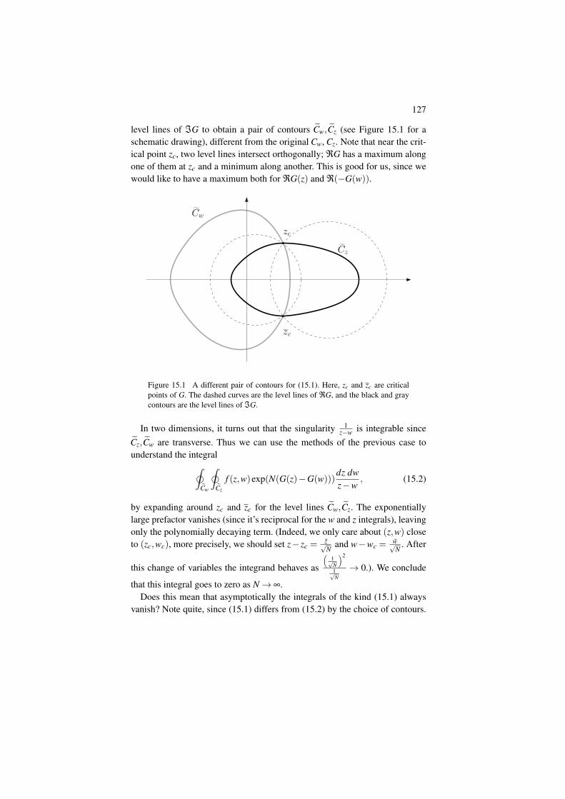
127
level lines of ℑG to obtain a pair of contours Cw,Cz (see Figure 15.1 for aschematic drawing), different from the original Cw, Cz. Note that near the crit-ical point zc, two level lines intersect orthogonally; ℜG has a maximum alongone of them at zc and a minimum along another. This is good for us, since wewould like to have a maximum both for ℜG(z) and ℜ(−G(w)).
Cw
Cz
zc
zc
Figure 15.1 A different pair of contours for (15.1). Here, zc and zc are criticalpoints of G. The dashed curves are the level lines of ℜG, and the black and graycontours are the level lines of ℑG.
In two dimensions, it turns out that the singularity 1z−w is integrable since
Cz,Cw are transverse. Thus we can use the methods of the previous case tounderstand the integral
˛Cw
˛Cz
f (z,w)exp(N(G(z)−G(w)))dz dwz−w
, (15.2)
by expanding around zc and zc for the level lines Cw,Cz. The exponentiallylarge prefactor vanishes (since it’s reciprocal for the w and z integrals), leavingonly the polynomially decaying term. (Indeed, we only care about (z,w) closeto (zc,wc), more precisely, we should set z− zc =
z√N
and w−wc =w√N
. After
this change of variables the integrand behaves as
(1√N
)2
1√N
→ 0.). We conclude
that this integral goes to zero as N→ ∞.Does this mean that asymptotically the integrals of the kind (15.1) always
vanish? Note quite, since (15.1) differs from (15.2) by the choice of contours.
128 Lecture 15: Steepest descent method for asymptotic analysis.
Hence, we should account for additional residues which might arise in the con-tour deformation. If we go back to the setting of Theorem 14.1, when we seethat the original contours are disjoint, while the new ones intersect. Hence, inthe deformation we pick up the residue at z = w arising from the 1
z−w factor inthe integrand. In principle, we might have needed to cross other poles, comingfrom the remaining factors of the integrand. Yet, let us assume that this is nothappening. Then we can conclude˛
Cw
˛Cz
f (z,w)exp(N(G(z)−G(w)))dz dwz−w
=
ˆ zc
zc
Resz=w dz+O(
1√N
),
where the integral is over the part of Cz between zc and zc. If the factor f (z,w)in (15.1) is non-singular, then the residue at z = w is equal to f (z,z), whichneeds to be integrated from zc to zc. This integral gives the leading asymptoticof (15.1).
Lecture 16: Bulk local limits for tilings ofhexagons
In this lecture, we use the material of the previous few lectures to find theasymptotic for the correlation functions of uniformly random tilings near apoint of a large hexagonal domain. Specifically, we apply the steepest descenttechniques of the previous lecture to find the asymptotic of the double contourintegral formula for the entries of the inverse Kasteleyn matrix from Lecture14.
Recall that we use shifted coordinates, so that the hexagonal domain hastwo horizontal and two vertical edges. For simplicity we consider a hexagonwith all side lengths N/2. Let us relate the trapezoids (or sawtooth domains)studied in previous lectures to the hexagons. If we consider a trapezoid withall dents located in the extreme rightmost and left-most positions along the topside (shown as solid black lozenges in Figure 16.1), then the lozenges belowthe dents are forced to be vertical (shown as outlined lozenges), and once allof these forced lozenges are removed, the domain becomes a hexagon.
For the desired N/2×N/2×N/2 hexagon, we choose its location such thatthe coordinates of the dents are −N/2,−N/2+1, . . . ,−1 for the dents on theright, and −3N/2, . . . ,−N−1 for the dents on the left.
Theorem 14.1 from Lecture 14 specializes to the following statement for thehexagon.1
Theorem 16.1 ([Petrov12a]). For even N consider the N/2× N/2× N/2
1 Another approach to explicit inversion of the Kasteleyn matrix for the hexagon is in[Gilmore17].
129
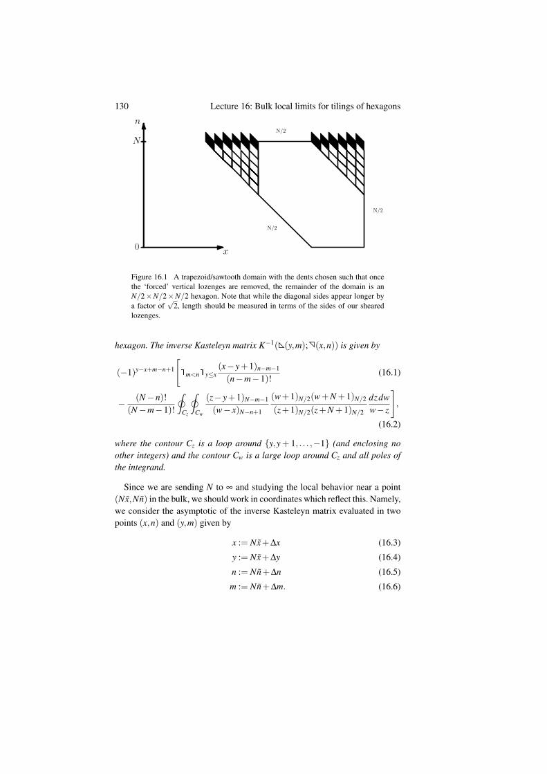
130 Lecture 16: Bulk local limits for tilings of hexagons
n
N
0 x
N/2
N/2
N/2
Figure 16.1 A trapezoid/sawtooth domain with the dents chosen such that oncethe ‘forced’ vertical lozenges are removed, the remainder of the domain is anN/2×N/2×N/2 hexagon. Note that while the diagonal sides appear longer bya factor of
√2, length should be measured in terms of the sides of our sheared
lozenges.
hexagon. The inverse Kasteleyn matrix K−1( (y,m); (x,n)) is given by
(−1)y−x+m−n+1
[1m<n1y≤x
(x− y+1)n−m−1
(n−m−1)!(16.1)
− (N−n)!(N−m−1)!
˛Cz
˛Cw
(z− y+1)N−m−1
(w− x)N−n+1
(w+1)N/2(w+N +1)N/2
(z+1)N/2(z+N +1)N/2
dzdww− z
],
(16.2)
where the contour Cz is a loop around y,y+ 1, . . . ,−1 (and enclosing noother integers) and the contour Cw is a large loop around Cz and all poles ofthe integrand.
Since we are sending N to ∞ and studying the local behavior near a point(Nx,Nn) in the bulk, we should work in coordinates which reflect this. Namely,we consider the asymptotic of the inverse Kasteleyn matrix evaluated in twopoints (x,n) and (y,m) given by
x := Nx+∆x (16.3)
y := Nx+∆y (16.4)
n := Nn+∆n (16.5)
m := Nn+∆m. (16.6)
131
The fact that x and y are both close to Nx, and similarly m,n are closeto Nn, guarantees that the points (x,n) and (y,m) stay close to (Nx,Nn).∆x,∆y,∆n,∆m control exactly where the two points sit relative to (Nx,Nn) ona local scale.
Here is our aim for this lecture:
Theorem 16.2. For (x, n) inside the liquid region (i.e. inside the ellipse in-scribed into the hexagon), the correlation functions of uniformly random tilingsof the hexagon converge to those of the ergodic translation-invariant Gibbsmeasure (see Lecture 13) associated to the slope of the limit shape at (x, n).
Remark 16.3. Since probabilities of the cylindrical events for random tilingscan be expressed as finite linear combinations of the correlation functions, theconvergence of the latter implies weak convergence of measures on tilings.
Proof of Theorem 16.2 Theorem 3.5 expresses the correlation functions oftilings through the inverse Kasteleyn matrix which is computed in Theorem16.1. We would like to apply the steepest descent method to the double con-tour integral in (16.2). For that we want to write the integrand of (16.2) asexp(N(G(z)−G(w))) ·O(1) for some function G, where (z,w) = (Nz,Nw).We set
G(z) =1N
N(1−n)
∑i=1
log(z−Nx+ i)− 1N
N/2
∑i=1
log(z+ i)− 1N
N/2
∑i=1
log(z+N + i)
(16.7)and note that
1N
N(1−n)
∑i=1
log(z−Nx+ i)− logN =1N
N(1−n)
∑i=1
log(z− x+iN) (16.8)
is a Riemann sum for´ 1−n
0 log(z− x+ u)du. Hence by subtracting one logNterm and adding two more to (16.7) to normalize the three sums as in (16.8),we obtain three Riemann sums corresponding to the three integral summandsin
G(z) :=ˆ 1−n
0log(z− x+u)du−
ˆ 1/2
0log(z+u)du−
ˆ 1/2
0log(z+1+u)du.
(16.9)It follows that
G(z) = G(z)+o(1)− logN, (16.10)
and the logN term will cancel in G(z)−G(w) so we may ignore it.For steepest descent analysis, we need the critical points of G. In order to
compute the derivative ∂ G∂ z , we differentiate under the integral sign, then take
132 Lecture 16: Bulk local limits for tilings of hexagons
the definite integral with respect to u which gives us back the logarithm, yield-ing
∂ G∂ z
= log(z− x+(1− n))− log(z− x)− log(z+1/2)
+ log(z)− log(z+3/2)+ log(z+1). (16.11)
Exponentiating we get a quadratic equation in z for the critical point:
∂ G∂ z
= 0 ⇐⇒ (z− x+(1− n))(z)(z+1) = (z− x)(z+1/2)(z+3/2)
(16.12)
⇐⇒ nz2− (x+14− n)z− 3
4x = 0. (16.13)
This equation has a pair of complex conjugate roots if and only if the discrim-inant is negative:
D = (x+1/4− n)2 +3nx < 0.
Remark 16.4. The region on the x, n coordinate plane given by (x+1/4− n)2+
3nx < 0 is exactly the interior of the inscribed ellipse of the hexagon of sidelengths 1/2 which is the scaled version of Figure 16.1. Clearly the equationcorresponds to a ellipse, and we can check that (x+1/4− n)2 +3nx = 0 has asingle solution (−3/4,1) when n= 1 and a single solution (−1/4,0) when n=0, corresponding to the tangency points at the top and bottom of the hexagon.The tangency points to other sides of the hexagon can be found similarly. Sincean ellipse is determined by five points, these tangency points fix the ellipseuniquely.
We assume that D < 0 and consider two conjugate critical points, zc and zc;this corresponds to (x, n) lying in the liquid region.
Next, we wish to find the steepest-descent contours for z and w. For that weconsider level lines of real and imaginary parts (ℜG(z) = const and ℑG(z) =const) passing through zc, zc. The latter will be the steepest descent contours,while the former will help us to understand their geometry. The schematicdrawing of the configuration of the level lines is shown in Figure 16.2. Thelevel lines of the real part, ℜG(z) = const, partition the Riemann sphere intoregions where ℜG(z)−ℜG(zc) is < 0 and > 0, represented by + and − in thefigure. Because G(z) decays as z→ ∞, the ‘outer’ region is a “−” region, andthis determines all the others since crossing a contour changes the sign.
There are two contours passing through zc and zc along which G(z) has con-stant imaginary part; one lies in the region of negative real part, the other inthe region of positive real part. However, the geometry of these contours is
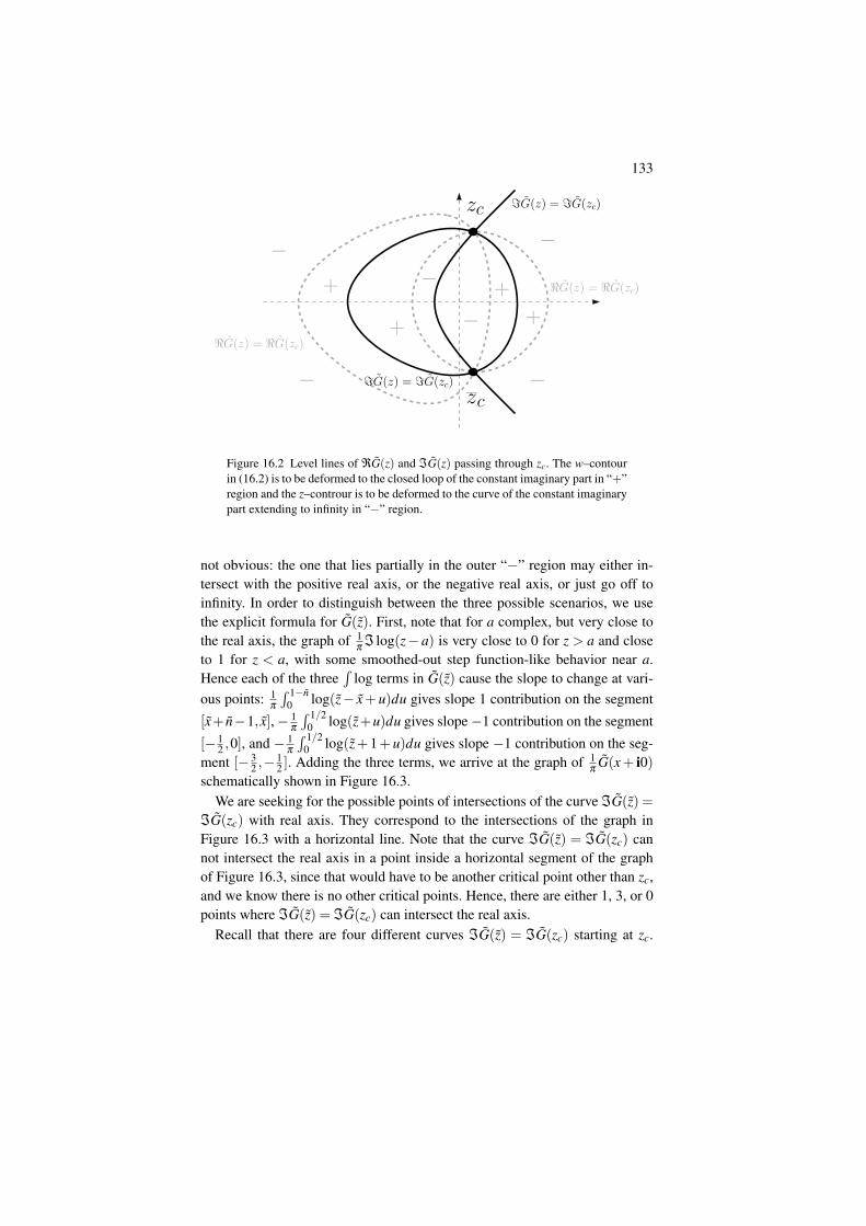
133
−
−−
−−
−+
+ +
+
=G(z) = =G(zc)
<G(z) = <G(zc)
zc
zc
<G(z) = <G(zc)
=G(z) = =G(zc)
Figure 16.2 Level lines of ℜG(z) and ℑG(z) passing through zc. The w–contourin (16.2) is to be deformed to the closed loop of the constant imaginary part in “+”region and the z–controur is to be deformed to the curve of the constant imaginarypart extending to infinity in “−” region.
not obvious: the one that lies partially in the outer “−” region may either in-tersect with the positive real axis, or the negative real axis, or just go off toinfinity. In order to distinguish between the three possible scenarios, we usethe explicit formula for G(z). First, note that for a complex, but very close tothe real axis, the graph of 1
πℑ log(z−a) is very close to 0 for z > a and close
to 1 for z < a, with some smoothed-out step function-like behavior near a.Hence each of the three
´log terms in G(z) cause the slope to change at vari-
ous points: 1π
´ 1−n0 log(z− x+u)du gives slope 1 contribution on the segment
[x+ n−1, x],− 1π
´ 1/20 log(z+u)du gives slope−1 contribution on the segment
[− 12 ,0], and − 1
π
´ 1/20 log(z+1+u)du gives slope −1 contribution on the seg-
ment [− 32 ,−
12 ]. Adding the three terms, we arrive at the graph of 1
πG(x+ i0)
schematically shown in Figure 16.3.We are seeking for the possible points of intersections of the curve ℑG(z) =
ℑG(zc) with real axis. They correspond to the intersections of the graph inFigure 16.3 with a horizontal line. Note that the curve ℑG(z) = ℑG(zc) cannot intersect the real axis in a point inside a horizontal segment of the graphof Figure 16.3, since that would have to be another critical point other than zc,and we know there is no other critical points. Hence, there are either 1, 3, or 0points where ℑG(z) = ℑG(zc) can intersect the real axis.
Recall that there are four different curves ℑG(z) = ℑG(zc) starting at zc.
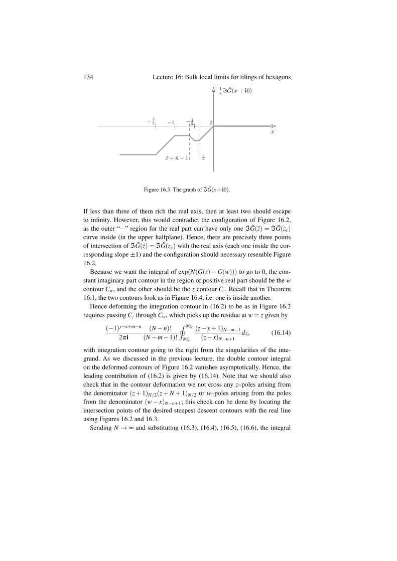
134 Lecture 16: Bulk local limits for tilings of hexagons
1π=G(x+ i0)
x
− 32 −1 − 1
2
xx+ n− 1
0
Figure 16.3 The graph of ℑG(x+ i0).
If less than three of them rich the real axis, then at least two should escapeto infinity. However, this would contradict the configuration of Figure 16.2,as the outer “−” region for the real part can have only one ℑG(z) = ℑG(zc)
curve inside (in the upper halfplane). Hence, there are precisely three pointsof intersection of ℑG(z) = ℑG(zc) with the real axis (each one inside the cor-responding slope ±1) and the configuration should necessary resemble Figure16.2.
Because we want the integral of exp(N(G(z)−G(w))) to go to 0, the con-stant imaginary part contour in the region of positive real part should be the wcontour Cw, and the other should be the z contour Cz. Recall that in Theorem16.1, the two contours look as in Figure 16.4, i.e. one is inside another.
Hence deforming the integration contour in (16.2) to be as in Figure 16.2requires passing Cz through Cw, which picks up the residue at w = z given by
(−1)y−x+m−n
2πi(N−n)!
(N−m−1)!
˛ Nzc
Nzc
(z− y+1)N−m−1
(z− x)N−n+1dz, (16.14)
with integration contour going to the right from the singularities of the inte-grand. As we discussed in the previous lecture, the double contour integralon the deformed contours of Figure 16.2 vanishes asymptotically. Hence, theleading contribution of (16.2) is given by (16.14). Note that we should alsocheck that in the contour deformation we not cross any z–poles arising fromthe denominator (z+ 1)N/2(z+N + 1)N/2 or w–poles arising from the polesfrom the denominator (w− x)N−n+1; this check can be done by locating theintersection points of the desired steepest descent contours with the real lineusing Figures 16.2 and 16.3.
Sending N → ∞ and substituting (16.3), (16.4), (16.5), (16.6), the integral
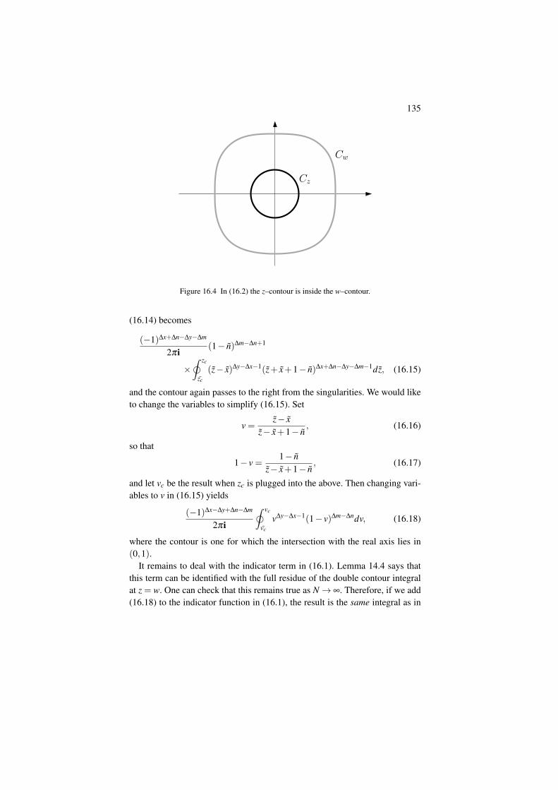
135
Cz
Cw
Figure 16.4 In (16.2) the z–contour is inside the w–contour.
(16.14) becomes
(−1)∆x+∆n−∆y−∆m
2πi(1− n)∆m−∆n+1
ײ zc
zc
(z− x)∆y−∆x−1(z+ x+1− n)∆x+∆n−∆y−∆m−1dz, (16.15)
and the contour again passes to the right from the singularities. We would liketo change the variables to simplify (16.15). Set
v =z− x
z− x+1− n, (16.16)
so that
1− v =1− n
z− x+1− n, (16.17)
and let vc be the result when zc is plugged into the above. Then changing vari-ables to v in (16.15) yields
(−1)∆x−∆y+∆n−∆m
2πi
˛ vc
vc
v∆y−∆x−1(1− v)∆m−∆ndv, (16.18)
where the contour is one for which the intersection with the real axis lies in(0,1).
It remains to deal with the indicator term in (16.1). Lemma 14.4 says thatthis term can be identified with the full residue of the double contour integralat z = w. One can check that this remains true as N→ ∞. Therefore, if we add(16.18) to the indicator function in (16.1), the result is the same integral as in
136 Lecture 16: Bulk local limits for tilings of hexagons
(16.18), except that the integration contour intersects the real axis on (0,1) for∆m≥ ∆n, and intersects on (−∞,0) for ∆m < ∆n, which is when the indicatorfunction is nonzero. This gives us the limiting value of K−1.
Remark 16.5. The limiting kernel which we just found, was first introducedby Okounkov and Reshetikhin in [OkounkovReshetikhin01]. It is called theincomplete beta kernel (since the integrand is the same as in the classical Betaintegral) or extended sine kernel. Here is the reason for the latter terminology.
If we set ∆m = ∆n in (16.18), then it becomes
(−1)∆x−∆y
2πi
˛ vc
vc
v∆y−∆x−1dv. (16.19)
Since the inverse Kasteleyn matrix is encoding probabilities of observinglozenges of different types, for any set of k points with the same n-coordinateand x-coordinates x1, . . . ,xn, the probability of observing a vertical lozenge(i.e., of left-most type in bottom-right panel of Figure 14.2) at each of the kpoints is det(K(xi− x j))1≤i, j≤k where
K(x) =(−1)x
2πi
ˆ vc
vc
vx−1dv = (−1)x (vc)x− vc
x
2πix=
(−|vc|)x
πxsin(xArg(vc)).
(16.20)The (−|vc|)x factor cancels in det(K(xi−x j))1≤i, j≤k and therefore, we can omitit. The conclusion is that the correlation functions of vertical lozenges along ahorizontal slice are given by the minors of the matrix
K(x) =
sin p1πx
πx , x 6= 0,
p1, x = 0,
where p1 is the asymptotic density of the vertical lozenges. We recognize thediscrete sine-kernel, which already appeared before in Corollary 13.16. Hencethe kernel of (16.18) yields the discrete sine kernel when restricted to a line,which is the origin of the name extended sine kernel.
Exercise 16.6. Show that the measure on lozenge tilings of the plane withcorrelation functions given by the minors of the extended sine kernel (16.18)(with the choice of integration contour described in the paragraph after theformula) is the same as one coming from the ergodic translation-invariantGibbs measure of Lecture 13 with slope corresponding to vc. Note that ourways of drawing lozenges differ between this lecture and Lecture 13, since weused affine-transformed coordinate system starting from Figure 14.2 in orderto match the notations of [Petrov12a].
This check is a more general version of the argument in Remark 16.5.
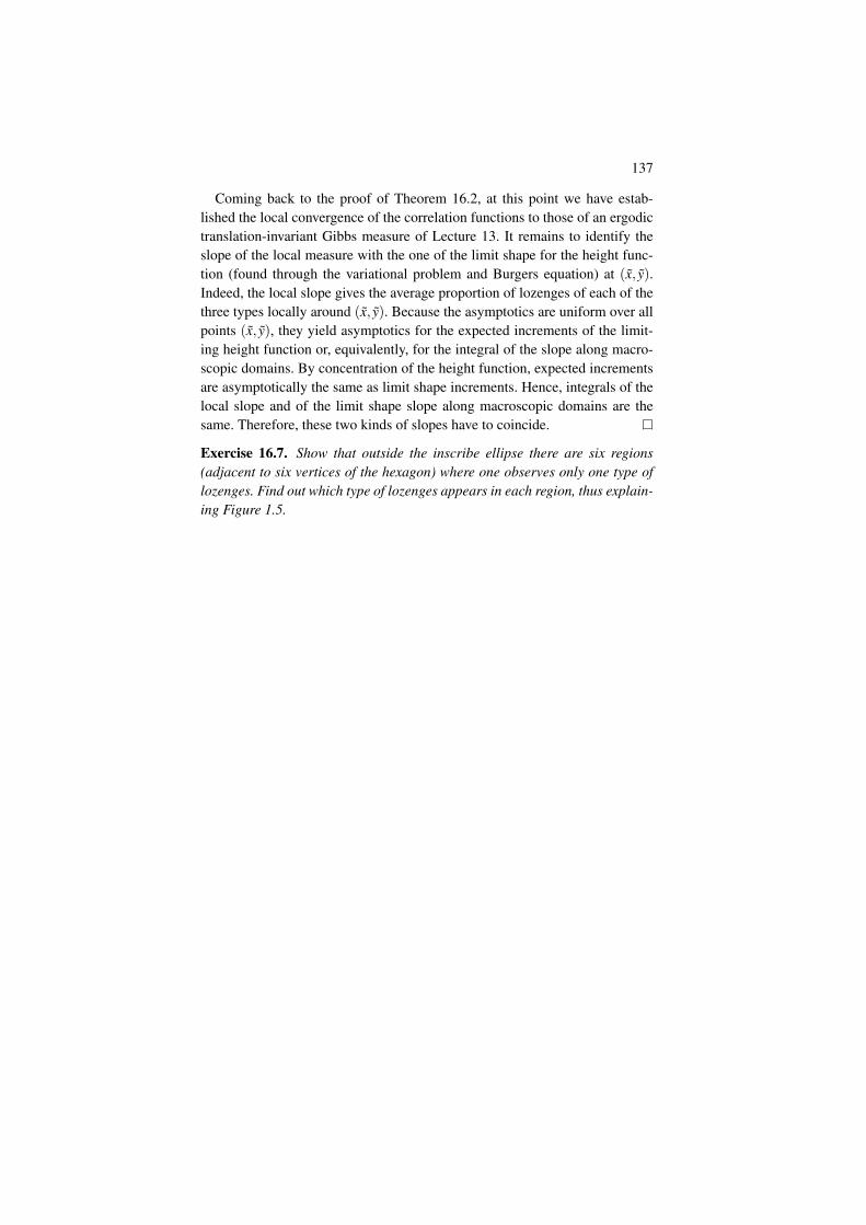
137
Coming back to the proof of Theorem 16.2, at this point we have estab-lished the local convergence of the correlation functions to those of an ergodictranslation-invariant Gibbs measure of Lecture 13. It remains to identify theslope of the local measure with the one of the limit shape for the height func-tion (found through the variational problem and Burgers equation) at (x, y).Indeed, the local slope gives the average proportion of lozenges of each of thethree types locally around (x, y). Because the asymptotics are uniform over allpoints (x, y), they yield asymptotics for the expected increments of the limit-ing height function or, equivalently, for the integral of the slope along macro-scopic domains. By concentration of the height function, expected incrementsare asymptotically the same as limit shape increments. Hence, integrals of thelocal slope and of the limit shape slope along macroscopic domains are thesame. Therefore, these two kinds of slopes have to coincide.
Exercise 16.7. Show that outside the inscribe ellipse there are six regions(adjacent to six vertices of the hexagon) where one observes only one type oflozenges. Find out which type of lozenges appears in each region, thus explain-ing Figure 1.5.
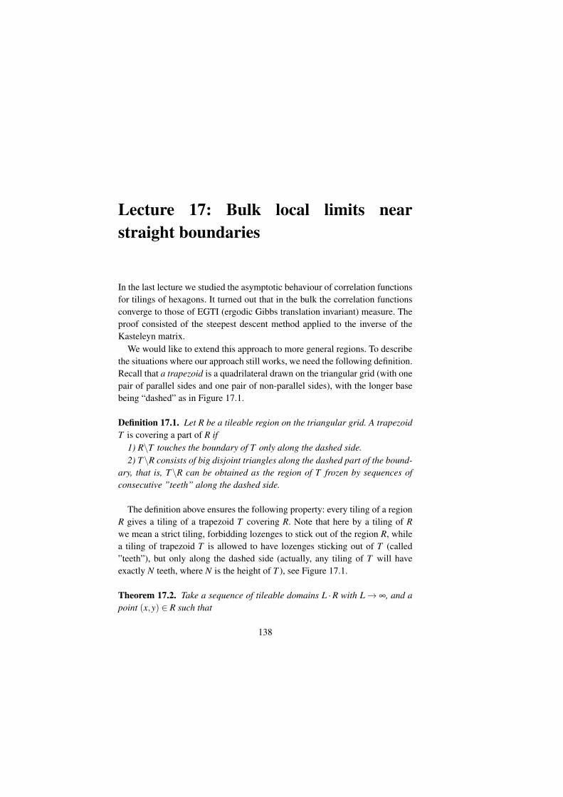
Lecture 17: Bulk local limits nearstraight boundaries
In the last lecture we studied the asymptotic behaviour of correlation functionsfor tilings of hexagons. It turned out that in the bulk the correlation functionsconverge to those of EGTI (ergodic Gibbs translation invariant) measure. Theproof consisted of the steepest descent method applied to the inverse of theKasteleyn matrix.
We would like to extend this approach to more general regions. To describethe situations where our approach still works, we need the following definition.Recall that a trapezoid is a quadrilateral drawn on the triangular grid (with onepair of parallel sides and one pair of non-parallel sides), with the longer basebeing “dashed” as in Figure 17.1.
Definition 17.1. Let R be a tileable region on the triangular grid. A trapezoidT is covering a part of R if
1) R\T touches the boundary of T only along the dashed side.2) T\R consists of big disjoint triangles along the dashed part of the bound-
ary, that is, T\R can be obtained as the region of T frozen by sequences ofconsecutive ”teeth” along the dashed side.
The definition above ensures the following property: every tiling of a regionR gives a tiling of a trapezoid T covering R. Note that here by a tiling of Rwe mean a strict tiling, forbidding lozenges to stick out of the region R, whilea tiling of trapezoid T is allowed to have lozenges sticking out of T (called”teeth”), but only along the dashed side (actually, any tiling of T will haveexactly N teeth, where N is the height of T ), see Figure 17.1.
Theorem 17.2. Take a sequence of tileable domains L ·R with L→ ∞, and apoint (x,y) ∈ R such that
138
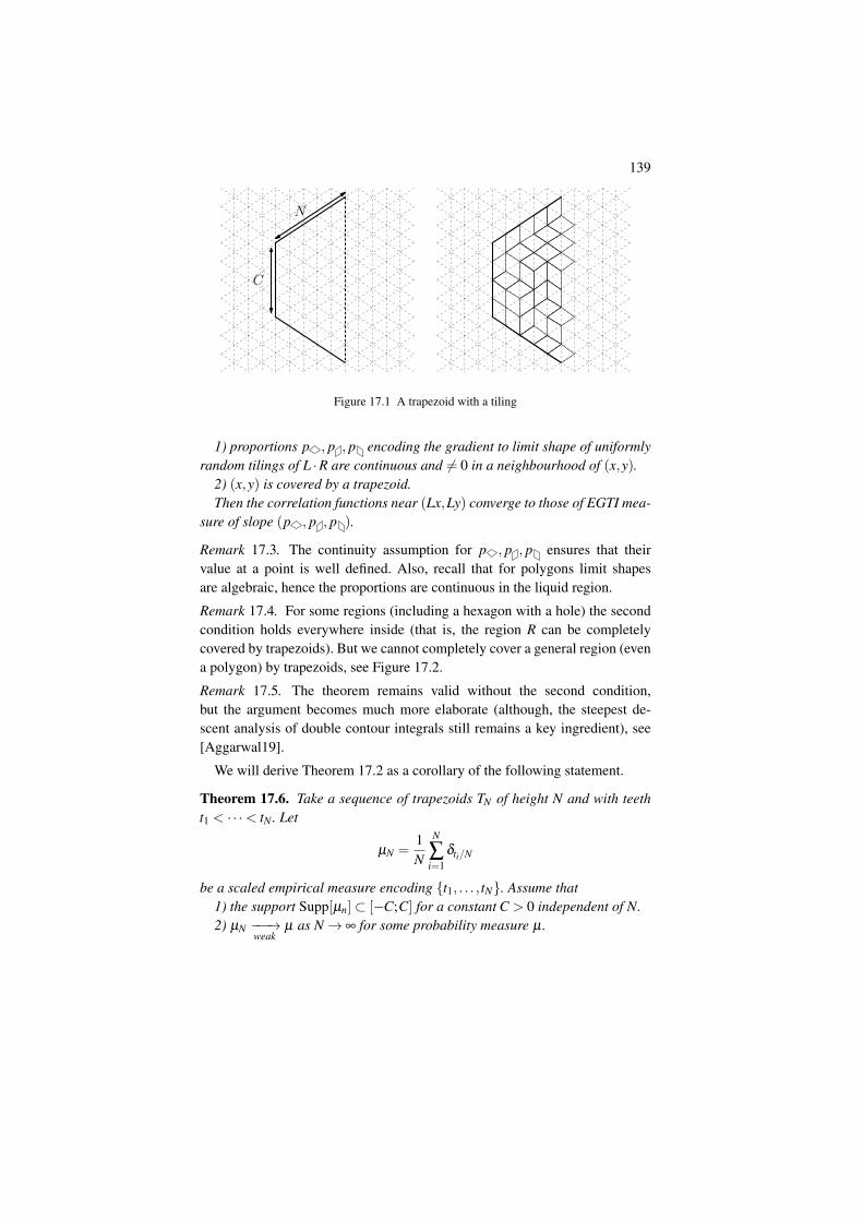
139
N
C
Figure 17.1 A trapezoid with a tiling
1) proportions p , p , p encoding the gradient to limit shape of uniformlyrandom tilings of L ·R are continuous and 6= 0 in a neighbourhood of (x,y).
2) (x,y) is covered by a trapezoid.Then the correlation functions near (Lx,Ly) converge to those of EGTI mea-
sure of slope (p , p , p ).
Remark 17.3. The continuity assumption for p , p , p ensures that theirvalue at a point is well defined. Also, recall that for polygons limit shapesare algebraic, hence the proportions are continuous in the liquid region.
Remark 17.4. For some regions (including a hexagon with a hole) the secondcondition holds everywhere inside (that is, the region R can be completelycovered by trapezoids). But we cannot completely cover a general region (evena polygon) by trapezoids, see Figure 17.2.
Remark 17.5. The theorem remains valid without the second condition,but the argument becomes much more elaborate (although, the steepest de-scent analysis of double contour integrals still remains a key ingredient), see[Aggarwal19].
We will derive Theorem 17.2 as a corollary of the following statement.
Theorem 17.6. Take a sequence of trapezoids TN of height N and with teetht1 < · · ·< tN . Let
µN =1N
N
∑i=1
δti/N
be a scaled empirical measure encoding t1, . . . , tN. Assume that1) the support Supp[µn]⊂ [−C;C] for a constant C > 0 independent of N.2) µN −−−→
weakµ as N→ ∞ for some probability measure µ .
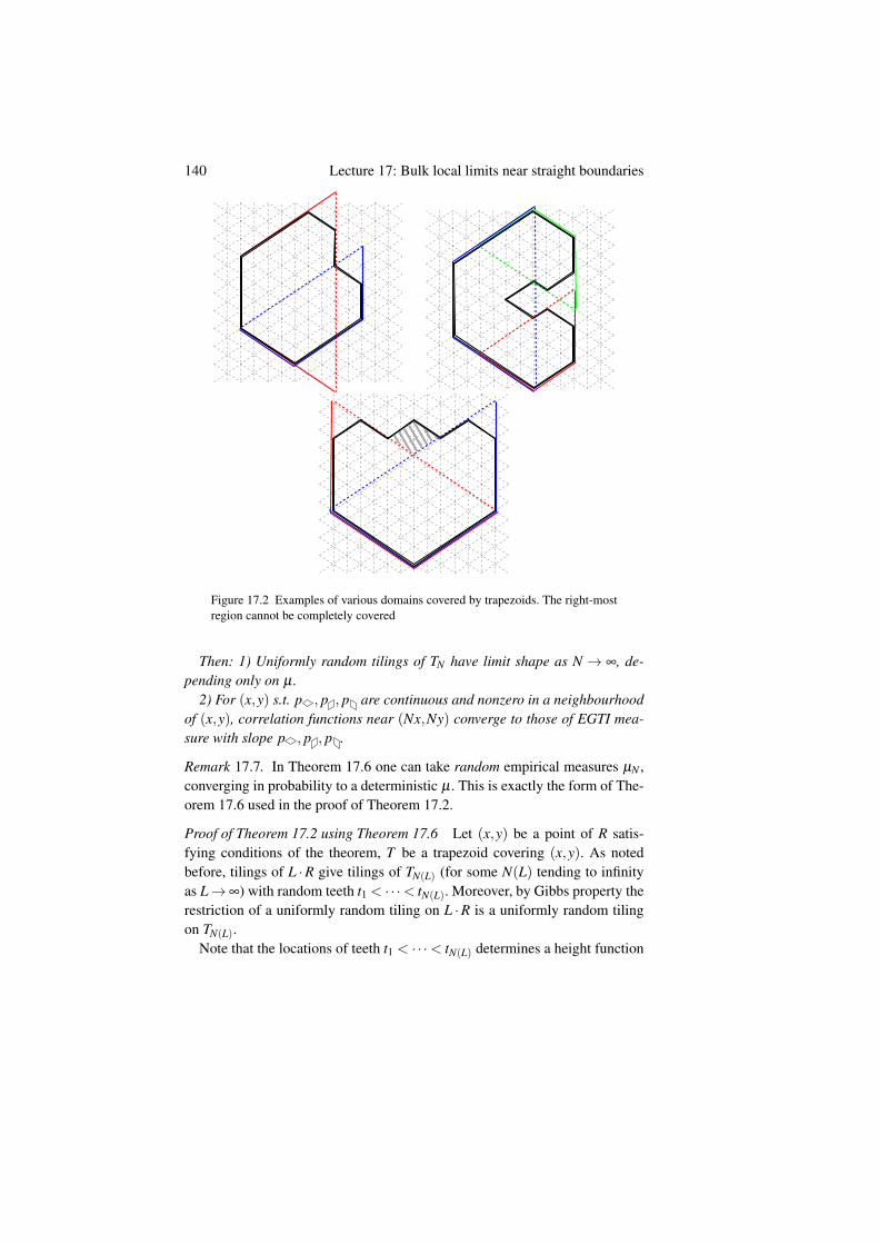
140 Lecture 17: Bulk local limits near straight boundaries
Figure 17.2 Examples of various domains covered by trapezoids. The right-mostregion cannot be completely covered
Then: 1) Uniformly random tilings of TN have limit shape as N → ∞, de-pending only on µ .
2) For (x,y) s.t. p , p , p are continuous and nonzero in a neighbourhoodof (x,y), correlation functions near (Nx,Ny) converge to those of EGTI mea-sure with slope p , p , p .
Remark 17.7. In Theorem 17.6 one can take random empirical measures µN ,converging in probability to a deterministic µ . This is exactly the form of The-orem 17.6 used in the proof of Theorem 17.2.
Proof of Theorem 17.2 using Theorem 17.6 Let (x,y) be a point of R satis-fying conditions of the theorem, T be a trapezoid covering (x,y). As notedbefore, tilings of L ·R give tilings of TN(L) (for some N(L) tending to infinityas L→∞) with random teeth t1 < · · ·< tN(L). Moreover, by Gibbs property therestriction of a uniformly random tiling on L ·R is a uniformly random tilingon TN(L).
Note that the locations of teeth t1 < · · ·< tN(L) determines a height function
141
hL along the dashed side of TN up to a constant, and µN(L) is the distribution ofhL(Lx,Ly)
L . Since uniformly random tilings of R converge to a deterministic limitshape, random functions hL(Lx,Ly)
L converge to a deterministic function h andhence the corresponding measures µN(L) converge to a deterministic measureµ . Also, note that the length of the dashed side of TN(L) grow linearly as L→∞,hence the support of measures µN(L) is inside [−C;C] for some C > 0.
So, both assumptions of Theorem 17.6 hold, hence the correlation functionsof uniformly random tilings near (Lx,Ly) converge to those of EGTI with thesame slope.
Proof of Theorem 17.6 For the first part note that the convergence of mea-sures µn imply the convergence of height functions on the dashed side of theboundary, hence height functions on the boundaries of TN converge and wehave a limit shape.
The proof of the second part is similar to the hexagon case (which is a partic-ular case where all teeth are concentrated near end-points of the dashed side):we study the asymptotic behaviour of the correlation kernel K−1((y,m),(x,n))using the steepest descent method. Here we cover only the main differencesfrom the hexagon case, for the full detailed exposition see [Gorin16].
Recall that the correlation kernel is given by the inverse Kasteleyn matrix
(−1)y−x+m−nK−1((y,m),(x,n)) =−1m<n1y≤x(x− y+1)n−m−1
(n−m−1)!
+(N−n)!
(N−m−1)!
˛C(y,...,t1−1)
dz˛
C(∞)dw
1w− z
(z− y+1)N−m−1
(w− x)N−n+1
N
∏i=1
w− tiz− ti
.
The behaviour of the indicator part is the same as in the hexagon case, sowe will focus on the double integral. Let T denote the set t1, . . . , tN andT = Z\T . Then the integrant has the form
1(w− x)(w− x+N−n)
exp(G1(z)−G2(w))(w− z)
where
G1(z) =− ∑t∈T
ln(z− t)+y−1
∑i=y−N+m
ln(z− i)
=− ∑d∈T \[y−N+m;y−1]
ln(z−d) + ∑d′∈[y−N+m;y−1]∩T
ln(z−d′)
and G2(w) is the same as G1(z) with y,m replaced by x,n.Recall that in order to use the steepest descent method we want to find suit-
able contours s.t. the exponent will be negative and the whole expression will
142 Lecture 17: Bulk local limits near straight boundaries
vanish as N → ∞. To do it, we have taken critical points of Gi as N → ∞,and constructed contours ℑ Gi = const passing through them. In the hexagoncase there were only two critical points, but now there can be more, makingthe construction of the contours seem more complicated. Fortunately, next twolemmas show that actually there are still no more than two nonreal criticalpoints.
Lemma 17.8. Equation G′1(z) = 0 has either 0 or 2 nonreal roots. Moreover,in the latter case the roots are complex conjugate.
Proof Rewrite G′1(z) = 0 as
∑d
1z−d
−∑d′
1z−d′
= 0. (17.1)
Let M denote the number of terms in (17.1). Multiplying (17.1) by a commondenominator, we get a degree M−1 polynomial with real coefficients. Henceall roots of G′1(z) = 0 are either real or form pairs of complex conjugate roots.So it is enough to show that there always are at least M−3 real roots.
Note that the restriction of −G′1(z) to the real line is a real function withM simple poles. Moreover, all poles outside of [y−N +m;y− 1] have posi-tive residues, while poles inside have negative residue. Then consecutive polesdi,di+1 s.t.
y−N +m 6∈ (di,di+1], y−1 6∈ [di,di+1)
have residues of the same sign. Since there are M−1 pairs of consecutive polesand only two pairs can violate condition on y− 1 and y−N +m above, thereare M− 3 pairs of consecutive poles with residues of the same sign. But anycontinuous real function has a zero between simple poles with the residues ofthe same sign. Hence −G′1(z) has M−3 real roots.
For N→ ∞ set
x = Nx+∆x, m = Nn+∆m,
y = Nx+∆y, n = Nn+∆n,
Let
G(z) =ˆ x
x+n−1ln(z− t)dt−
ˆR
ln(z− t)µ(t)dt.
Lemma 17.9. G(z) has either 0 or 2 complex conjugate roots.
143
Proof Note that
G′1(Nz) =− ∑t∈T
1N(z− t/N)
+y−1
∑i=y−N+m
1N(z− i/N)
Both sums are Riemann sums of integrals in
G′(z) =−ˆR
1z− t
µ(t)dt +ˆ x
x+n−1
1z− t
dt
hence G′1(Nz)⇒ G′(z) uniformly on compact subsets of C\R. Then by Hur-witz’s theorem the zeroes of G′1(Nz) converge to zeroes of G′(z), hence G hasno more than 2 complex conjugate critical points.
Call a pair (x, n) good if there are 2 complex conjugate critical points ofG(z), let τ(x, n) denote the critical point in the upper half-plane. Then 1
N Gi(Nz)converge to G(z) and as N→ ∞ we have
exp(G1(Nz)−G1(Nw))≈ exp(N(G(z)− G(w)))
Now we are in the same situation as in the last lecture and repeating the steepestdescent argument we get (after change of variables)
(−1)y−x+m−nK−1((y,m),(x,n))−→ 12πi
ˆξ
ξ
v∆y−∆x−1(1− v)∆m−∆ndv,
where ξ = τ−xτ−x+1−n and the contour between ξ and ξ intersects R in [0,1]
if ∆m ≥ ∆n or in (−∞;0) otherwise. As noted in the previous lecture, thisis exactly correlation kernel of EGTI measure. Moreover, in the end of theprevious lecture we proved that the slope of this EGTI measure must matchthe slope of the limit shape.
To finish the proof we must show that the ”good” points above (i.e. the pointss.t. τ(x, n) is well defined) are exactly the points s.t. the slope is nonextreme.Recall that the slope (p , p , p ) can be directly recovered from the correla-tion kernel by looking at the first correlation function, see Corollary 13.16 andRemark 13.17. The three components of the slope (which we intentionally donot write as , , here in order to avoid the confusion between two coordinatesystems in Lecture 13 and in Lectures 14,16) are
p1(x, n) = limN→∞
K−1((Nx,Nn),(Nx,Nn)) =1
2πi
ˆξ
ξ+v−1dv
=ln+(ξ )− ln+(ξ )
2πi=
Arg ξ
π
144 Lecture 17: Bulk local limits near straight boundaries
p2(x, n) = limN→∞
K−1((Nx−1,Nn+1),(Nx,Nn)) =1
2πi
ˆξ
ξ
(1− v)−1dv
=− ln+(1−ξ )+ ln+(1− ξ )
2πi=−Arg(1−ξ )
π
p3(x, n) = limN→∞
K−1((Nx,Nn+1),(Nx,Nn)) =− 12πi
ˆξ
ξ
v−1(1− v)−1dv
=−ln−( ξ
1−ξ)− ln−( ξ
1−ξ)
2πi= 1−
Arg( ξ
1−ξ)
π.
(the contours pass through [0,1] in the first case and through (−∞,0) in the sec-ond and third cases, ln+(z) is a branch of ln(z) defined on C\(−∞;0), ln−(z)is a branch defined on C\(0,∞)).
This computation shows that the three components of the slope (multipliedby Π) are precisely the angles of the triangle with vertices 0,1,ξ (and therefore,ξ is the Kenyon-Okounkov cooridnate). Hence for a “good”, ξ is complex andthe slope is nonextreme. For the other direction see [Gorin16].
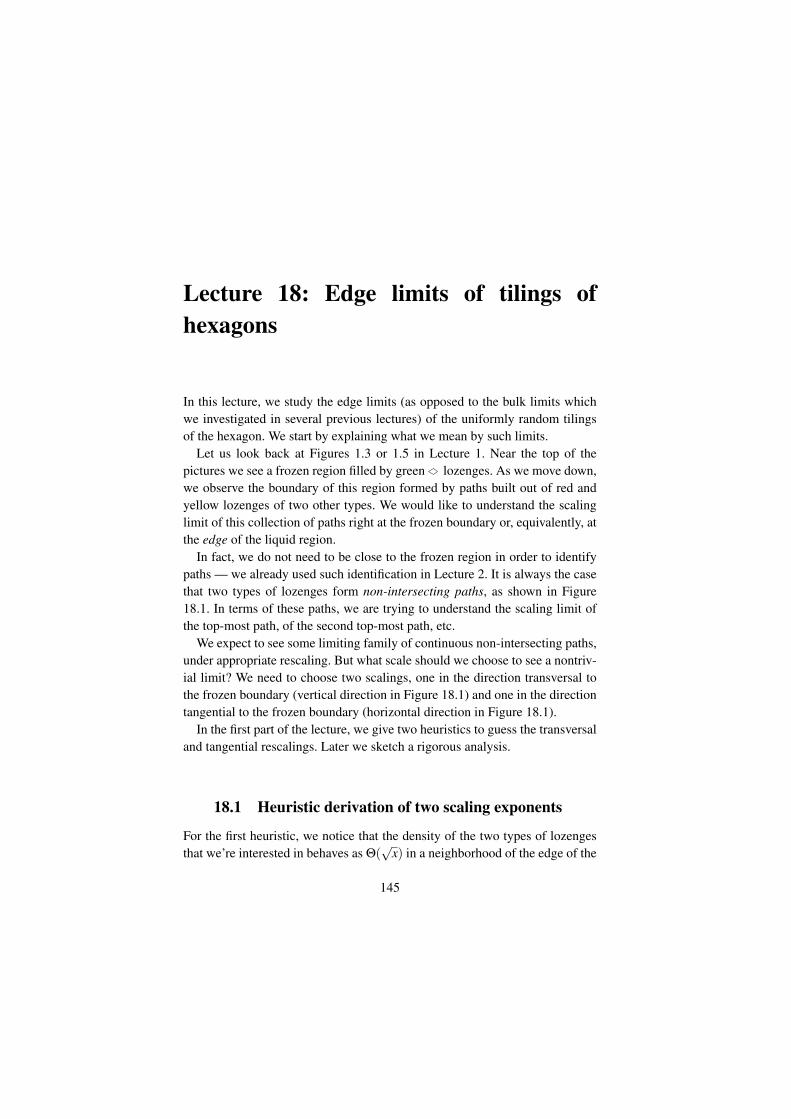
Lecture 18: Edge limits of tilings ofhexagons
In this lecture, we study the edge limits (as opposed to the bulk limits whichwe investigated in several previous lectures) of the uniformly random tilingsof the hexagon. We start by explaining what we mean by such limits.
Let us look back at Figures 1.3 or 1.5 in Lecture 1. Near the top of thepictures we see a frozen region filled by green lozenges. As we move down,we observe the boundary of this region formed by paths built out of red andyellow lozenges of two other types. We would like to understand the scalinglimit of this collection of paths right at the frozen boundary or, equivalently, atthe edge of the liquid region.
In fact, we do not need to be close to the frozen region in order to identifypaths — we already used such identification in Lecture 2. It is always the casethat two types of lozenges form non-intersecting paths, as shown in Figure18.1. In terms of these paths, we are trying to understand the scaling limit ofthe top-most path, of the second top-most path, etc.
We expect to see some limiting family of continuous non-intersecting paths,under appropriate rescaling. But what scale should we choose to see a nontriv-ial limit? We need to choose two scalings, one in the direction transversal tothe frozen boundary (vertical direction in Figure 18.1) and one in the directiontangential to the frozen boundary (horizontal direction in Figure 18.1).
In the first part of the lecture, we give two heuristics to guess the transversaland tangential rescalings. Later we sketch a rigorous analysis.
18.1 Heuristic derivation of two scaling exponents
For the first heuristic, we notice that the density of the two types of lozengesthat we’re interested in behaves as Θ(
√x) in a neighborhood of the edge of the
145
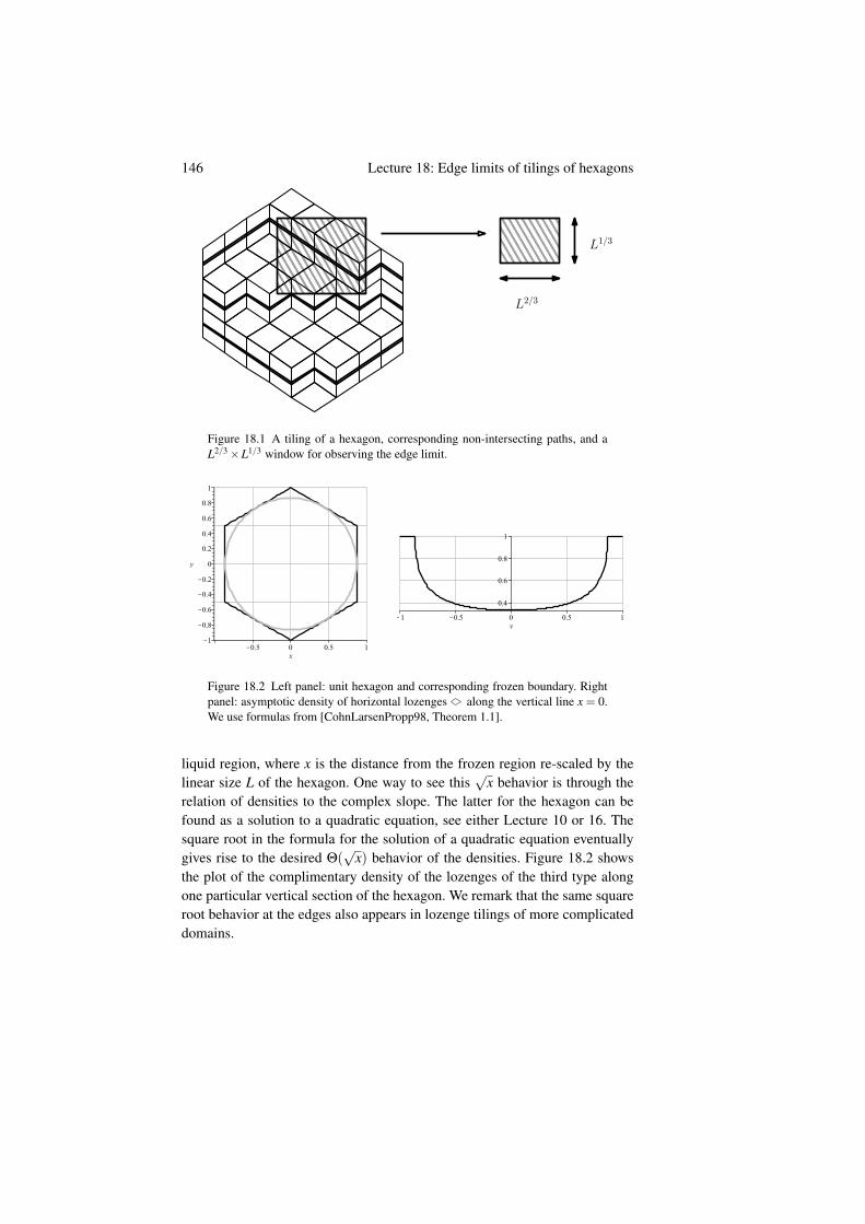
146 Lecture 18: Edge limits of tilings of hexagons
L1/3
L2/3
Figure 18.1 A tiling of a hexagon, corresponding non-intersecting paths, and aL2/3×L1/3 window for observing the edge limit.
Figure 18.2 Left panel: unit hexagon and corresponding frozen boundary. Rightpanel: asymptotic density of horizontal lozenges along the vertical line x = 0.We use formulas from [CohnLarsenPropp98, Theorem 1.1].
liquid region, where x is the distance from the frozen region re-scaled by thelinear size L of the hexagon. One way to see this
√x behavior is through the
relation of densities to the complex slope. The latter for the hexagon can befound as a solution to a quadratic equation, see either Lecture 10 or 16. Thesquare root in the formula for the solution of a quadratic equation eventuallygives rise to the desired Θ(
√x) behavior of the densities. Figure 18.2 shows
the plot of the complimentary density of the lozenges of the third type alongone particular vertical section of the hexagon. We remark that the same squareroot behavior at the edges also appears in lozenge tilings of more complicateddomains.
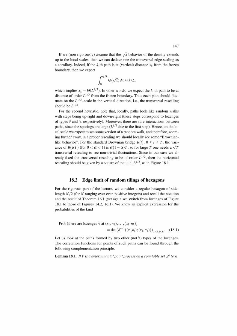
147
If we (non-rigorously) assume that the√
x behavior of the density extendsup to the local scales, then we can deduce one the transversal edge scaling asa corollary. Indeed, if the k-th path is at (vertical) distance xk from the frozenboundary, then we expect
ˆ xk/L
0Θ(√
x)dx≈ k/L,
which implies xk = Θ(L1/3). In other words, we expect the k–th path to be atdistance of order L1/3 from the frozen boundary. Thus each path should fluc-tuate on the L1/3–scale in the vertical direction, i.e., the transversal rescalingshould be L1/3.
For the second heuristic, note that, locally, paths look like random walkswith steps being up-right and down-right (these steps correspond to lozengesof types and , respectively). Moreover, there are rare interactions betweenpaths, since the spacings are large (L1/3 due to the first step). Hence, on the lo-cal scale we expect to see some version of a random walk, and therefore, zoom-ing further away, in a proper rescaling we should locally see some “Brownian-like behavior”. For the standard Brownian bridge B(t), 0 ≤ t ≤ T , the vari-ance of B(αT ) (for 0 < α < 1) is α(1−α)T , so for large T one needs a
√T
transversal rescaling to see non-trivial fluctuations. Since in our case we al-ready fixed the transversal rescaling to be of order L1/3, then the horizontalrescaling should be given by a square of that, i.e. L2/3, as in Figure 18.1.
18.2 Edge limit of random tilings of hexagons
For the rigorous part of the lecture, we consider a regular hexagon of side-length N/2 (for N ranging over even positive integers) and recall the notationand the result of Theorem 16.1 (yet again we switch from lozenges of Figure18.1 to those of Figures 14.2, 16.1). We know an explicit expression for theprobabilities of the kind
Prob(there are lozenges at (x1,n1), . . . ,(xk,nk))
= det(K−1((xi,ni);(x j,n j))
)1≤i, j≤k . (18.1)
Let us look at the paths formed by two other (not ) types of the lozenges.The correlation functions for points of such paths can be found through thefollowing complementation principle.
Lemma 18.1. If P is a determinantal point process on a countable set L (e.g.,
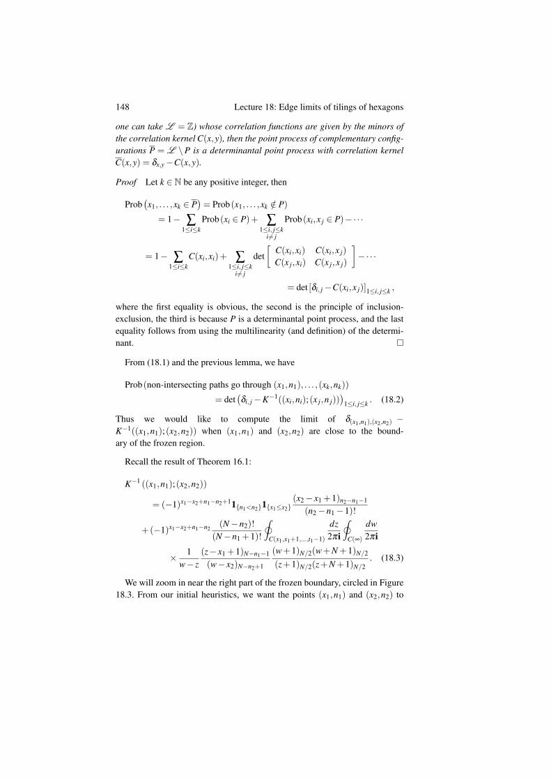
148 Lecture 18: Edge limits of tilings of hexagons
one can take L = Z) whose correlation functions are given by the minors ofthe correlation kernel C(x,y), then the point process of complementary config-urations P = L \P is a determinantal point process with correlation kernelC(x,y) = δx,y−C(x,y).
Proof Let k ∈ N be any positive integer, then
Prob(x1, . . . ,xk ∈ P
)= Prob(x1, . . . ,xk /∈ P)
= 1− ∑1≤i≤k
Prob(xi ∈ P)+ ∑1≤i, j≤k
i6= j
Prob(xi,x j ∈ P)−·· ·
= 1− ∑1≤i≤k
C(xi,xi)+ ∑1≤i, j≤k
i6= j
det[
C(xi,xi) C(xi,x j)
C(x j,xi) C(x j,x j)
]−·· ·
= det [δi, j−C(xi,x j)]1≤i, j≤k ,
where the first equality is obvious, the second is the principle of inclusion-exclusion, the third is because P is a determinantal point process, and the lastequality follows from using the multilinearity (and definition) of the determi-nant.
From (18.1) and the previous lemma, we have
Prob(non-intersecting paths go through (x1,n1), . . . ,(xk,nk))
= det(δi, j−K−1((xi,ni);(x j,n j))
)1≤i, j≤k . (18.2)
Thus we would like to compute the limit of δ(x1,n1),(x2,n2) −K−1((x1,n1);(x2,n2)) when (x1,n1) and (x2,n2) are close to the bound-ary of the frozen region.
Recall the result of Theorem 16.1:
K−1 ((x1,n1);(x2,n2))
= (−1)x1−x2+n1−n2+11n1<n21x1≤x2(x2− x1 +1)n2−n1−1
(n2−n1−1)!
+(−1)x1−x2+n1−n2(N−n2)!
(N−n1 +1)!
˛C(x1,x1+1,...,t1−1)
dz2πi
˛C(∞)
dw2πi
× 1w− z
(z− x1 +1)N−n1−1
(w− x2)N−n2+1
(w+1)N/2(w+N +1)N/2
(z+1)N/2(z+N +1)N/2. (18.3)
We will zoom in near the right part of the frozen boundary, circled in Figure18.3. From our initial heuristics, we want the points (x1,n1) and (x2,n2) to
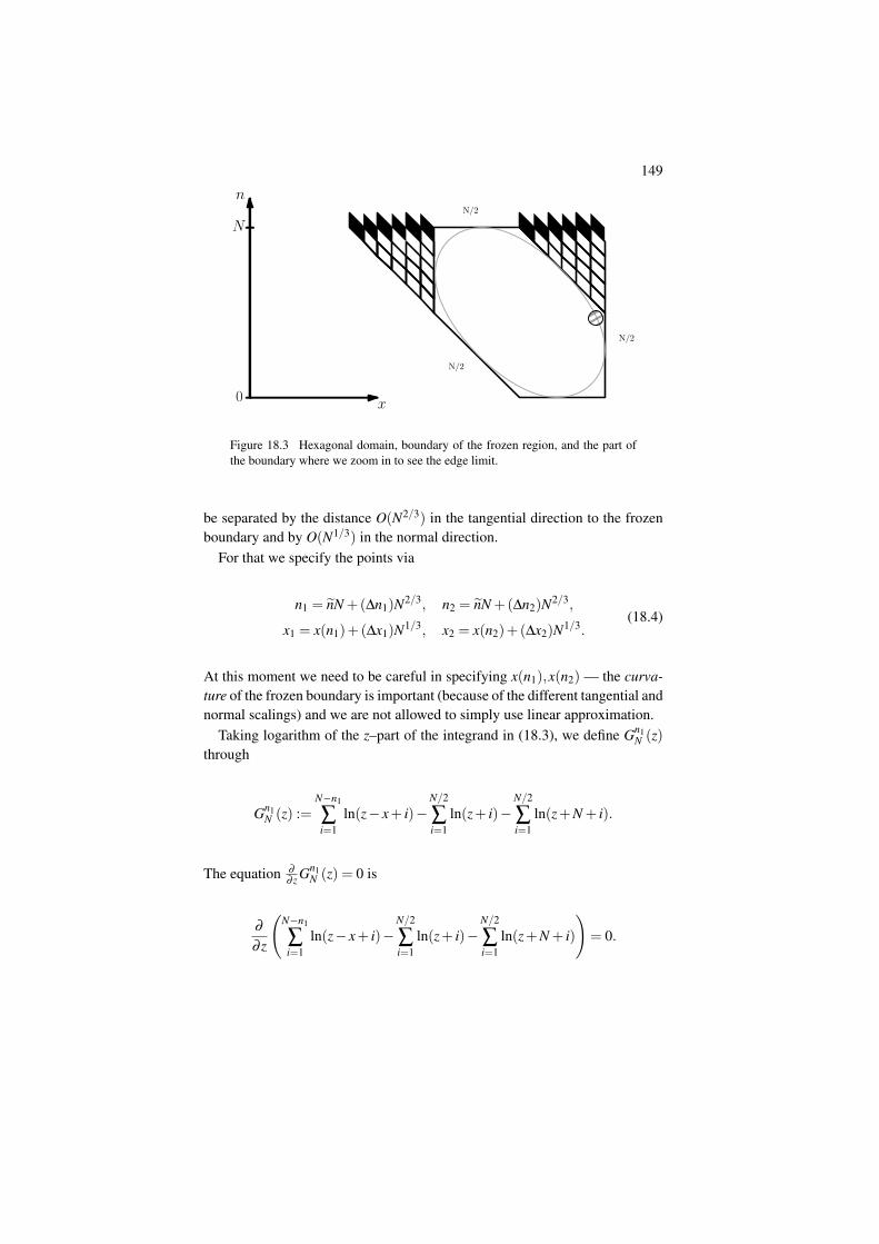
149
n
N
0 x
N/2
N/2
N/2
Figure 18.3 Hexagonal domain, boundary of the frozen region, and the part ofthe boundary where we zoom in to see the edge limit.
be separated by the distance O(N2/3) in the tangential direction to the frozenboundary and by O(N1/3) in the normal direction.
For that we specify the points via
n1 = nN +(∆n1)N2/3, n2 = nN +(∆n2)N2/3,
x1 = x(n1)+(∆x1)N1/3, x2 = x(n2)+(∆x2)N1/3.(18.4)
At this moment we need to be careful in specifying x(n1),x(n2) — the curva-ture of the frozen boundary is important (because of the different tangential andnormal scalings) and we are not allowed to simply use linear approximation.
Taking logarithm of the z–part of the integrand in (18.3), we define Gn1N (z)
through
Gn1N (z) :=
N−n1
∑i=1
ln(z− x+ i)−N/2
∑i=1
ln(z+ i)−N/2
∑i=1
ln(z+N + i).
The equation ∂
∂ z Gn1N (z) = 0 is
∂
∂ z
(N−n1
∑i=1
ln(z− x+ i)−N/2
∑i=1
ln(z+ i)−N/2
∑i=1
ln(z+N + i)
)= 0.
150 Lecture 18: Edge limits of tilings of hexagons
Instead of this equation, it is easier to consider its N→ ∞ approximation:
∂
∂ z
(ˆ 1− n1N
0ln( z
N− x
N+u)
du
−ˆ 1/2
0ln( z
N+u)
du−ˆ 1/2
0ln( z
N+1+u
)du
)= 0.
The above equation is quadratic in z and one needs to take x = x(n1) so thatthis equation has a double real root zc. The value of x(n2) is obtained throughthe same procedure.
The steepest descent analysis of the double contour integral is done similarlyto the bulk case, except that now two complex conjugate critical points mergeinto a single double critical point on the real axis. In the neighborhood of thecritical point we have
Gn1N (z)≈ Gn1
N (zc)+(z− zc)3α, (18.5)
for some explicit α .Previously, in the bulk analysis the steepest descent contours of integration
passed through two critical points, but now there is only one critical point zc,so the situation is degenerate. One can obtain the configuration of the contoursfor the present case by continuously deforming Figure 16.2 into the situationof merging critical points. The z contour should pass through zc and w contourshould pass through similarly defined wc (which is close to zc, since n2 is closeto n2) under such angles as to guarantee the negative real part of Gn1
N (z)−Gn2
N (w) after using (18.5) in a neighborhood of the critical point.For the limit, we zoom-in near the critical points, where the contours can
be chosen to look like in Figure 18.4. As in the bulk case, one also needs tomake sure that this local picture can be extended to the global steepest descentcontours (such that the real part of the exponent is still be maximized near thecritical point) — we omit this part of the argument. We reach the followingtheorem and refer to [Petrov12a, Section 8] for more details.
Theorem 18.2. In the limit regime (18.4), which describes the random lozengetiling near the boundary of the frozen region, we have
limN→∞
N1/3 (δ(x1,n1),(x2,n2)−K−1 ((x1,n1);(x2,n2))
)=A ((∆x1,∆n1);(∆x2,∆n2)) ,
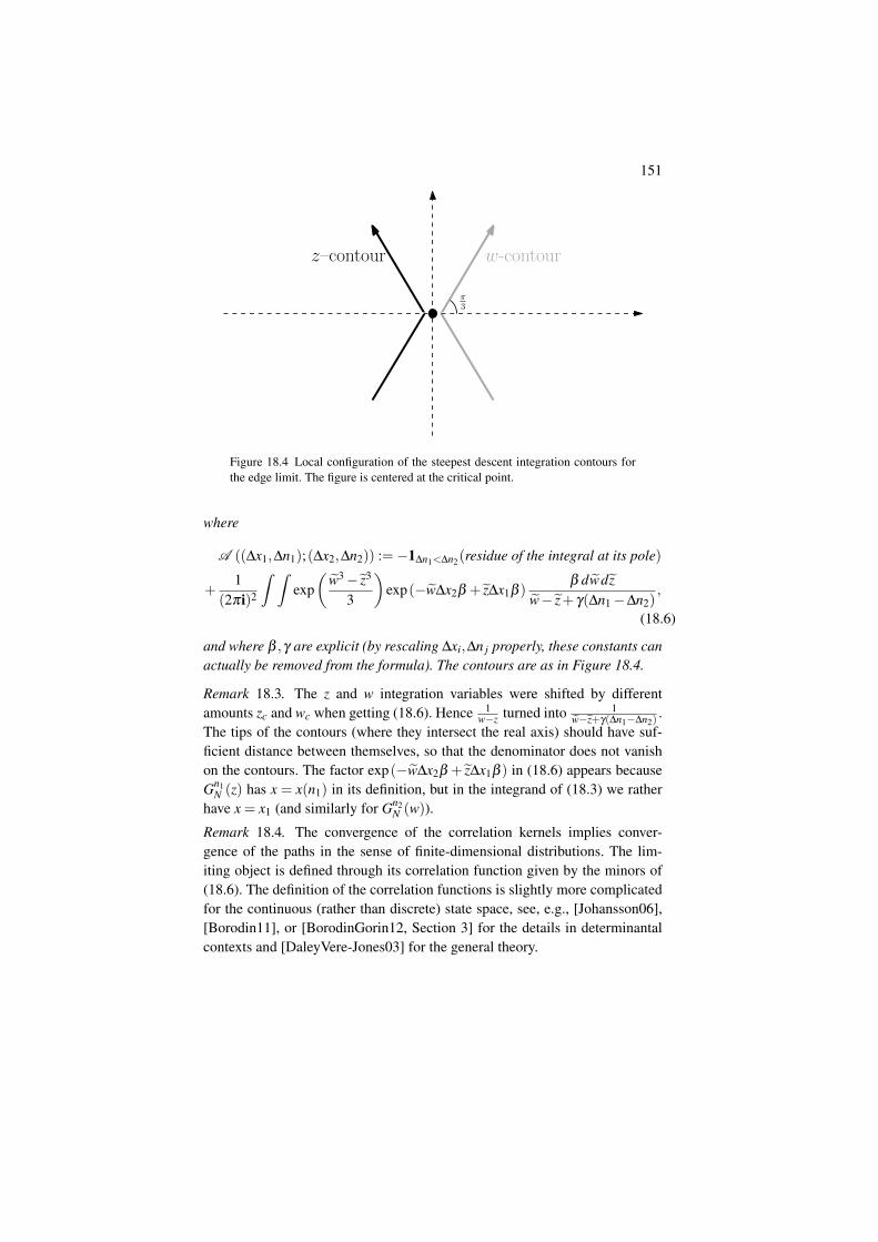
151
w-contourz–contour
π3
Figure 18.4 Local configuration of the steepest descent integration contours forthe edge limit. The figure is centered at the critical point.
where
A ((∆x1,∆n1);(∆x2,∆n2)) :=−1∆n1<∆n2(residue of the integral at its pole)
+1
(2πi)2
ˆ ˆexp(
w3− z3
3
)exp(−w∆x2β + z∆x1β )
β dwdzw− z+ γ(∆n1−∆n2)
,
(18.6)
and where β ,γ are explicit (by rescaling ∆xi,∆n j properly, these constants canactually be removed from the formula). The contours are as in Figure 18.4.
Remark 18.3. The z and w integration variables were shifted by differentamounts zc and wc when getting (18.6). Hence 1
w−z turned into 1w−z+γ(∆n1−∆n2)
.The tips of the contours (where they intersect the real axis) should have suf-ficient distance between themselves, so that the denominator does not vanishon the contours. The factor exp(−w∆x2β + z∆x1β ) in (18.6) appears becauseGn1
N (z) has x = x(n1) in its definition, but in the integrand of (18.3) we ratherhave x = x1 (and similarly for Gn2
N (w)).
Remark 18.4. The convergence of the correlation kernels implies conver-gence of the paths in the sense of finite-dimensional distributions. The lim-iting object is defined through its correlation function given by the minors of(18.6). The definition of the correlation functions is slightly more complicatedfor the continuous (rather than discrete) state space, see, e.g., [Johansson06],[Borodin11], or [BorodinGorin12, Section 3] for the details in determinantalcontexts and [DaleyVere-Jones03] for the general theory.
152 Lecture 18: Edge limits of tilings of hexagons
Exercise 18.5. Finish the proof of Theorem 18.2 and compute the values of β
and γ .
A rescaled version of the kernel A above is known as the extended Airykernel in the literature. Here is its standard form:
KAiryextended ((x, t);(y,s)) :=
´∞
0 e−λ (t−s)Ai(x+λ )Ai(y+λ )dλ , if t ≥ s,
−´ 0−∞
e−λ (t−s)Ai(x+λ )Ai(y+λ )dλ , if t < s,(18.7)
where
Ai(z) :=1
2πi
ˆexp(
v3
3− zv
)dv, (18.8)
is the Airy function1; the contour in the integral is the upwards-directed con-tour which is the union of the lines e−iπ/3t : t ≥ 0 and eiπ/3t : t ≥ 0 (itlooks like the w–contour in Figure 18.4).
Exercise 18.6. Match KAiryextended((x, t);(y,s)) with A ((x, t);(y,s)) in Theorem
18.2 by substituting (18.8) into (18.7), and explicitly evaluating the λ -integral.
The conclusion is that the ensembles of extreme paths (edge limit) in ran-dom tilings of large hexagons converge to the random path ensemble whosecorrelation functions are minors of the extended Airy kernel.
18.3 Airy line ensemble in tilings and beyond
It is believed that Theorem 18.2 is not specific to the hexagons.
Conjecture 18.7. The extended Airy kernel arises in the edge limit of the uni-form lozenge tilings of arbitrary polygonal domains, as the mesh size of thegrid goes to zero.
The conjecture has been proved in certain cases (for trapezoids) in[Petrov12a], [DuseMetcalfe17]. The first appearance of the extended Airy ker-nel is in [PrahoferSpohn01] in the study of the polynuclear growth model(PNG). Closer to the tilings context, [FerrariSpohn02] were first to find theextended Airy kernel in the edge limit of the qVolume–weighted plane parti-tions (we will discuss this model of random plane partitions in Lecture 22) and[Johansson05] found it in the domino tilings of the Aztec diamons.
1 Airy function solves the second order differential equation ∂ 2
∂ z2 Ai(z)− zAi(z) = 0.
153
The random two-dimensional ensemble (a random ensemble of paths) aris-ing from the extended Airy kernel is called the Airy line ensemble. It is atranslation-invariant ensemble (in the space direction). In the next lecture, wewill learn more about it and tie it to other subjects in probability. As a warm-up, let us mention that the one-point distribution of the “top-most” path isknown as the Tracy-Widom distribution2. This distribution also appears in var-ious other contexts:
1 In random matrix theory: the TW distribution is (the limit of) the dis-tribution of the largest eigenvalue of a large Hermitian random matricesof growing sizes, see reviews [Forrester10, AndersonGuionnetZeitouni10,AkemannBaikFrancesco11]. We are going to explain in more details the linkbetween tilings and random matrices in the next two lectures.
2 In interacting particle systems: the TW distribution arises as the limit-ing particle current for various systems, including the Totally AsymmetricSimple Exclusion Process (TASEP). We do not have time to discuss thedirect links between tilings and interacting particle systems in these lec-tures, and we instead only refer to reviews [Johansson06, BorodinGorin12,BorodinPetrov13, Romik15].
3 In directed polymers: the TW distribution governs the asymptotic law ofthe partition function for directed polymers in random media and relatedsolution of the Kardar–Parisi–Zhang stochastic partial differential equation,see reviews [Corwin11, QuastelSpohn15]
4 In asymptotic representation theory: the TW distribution is the asymp-totic law for the first row of random Young diagrams encoding decompo-sition of representations (typically of unitary or symmetric groups) into ir-reducible components. The most celebrated result of this kind deals withPlancherel measure for the symmetric groups, see reviews [Johansson06,BorodinGorin12, Romik15, BaikDeiftSuidan16].
2 The wikipedia page https://en.wikipedia.org/wiki/Tracy-Widom_distributionis a good initial source of the information
Lecture 19: Airy line ensemble, GUE-corners, and others
19.1 Invariant description of the Airy line ensemble
In the previous lecture we found Airy line ensemble as the edge limit of theuniformly random tilings of hexagons. We described it in terms of its correla-tion functions, which are minors of the extended Airy kernel of (18.7). On theother hand, in the bulk, we could describe the limiting object without formu-las: it was a unique Gibbs, translationally invariant, ergodic measure of a givenslope.
Is there a similar description for the Airy line ensemble?
Conjecturally, the answer is yes, based on the following three facts:(1) The Airy line ensemble is translationally invariant in the t (i.e., horizontal)direction — this immediately follows from (18.7).
(2) The Airy line ensemble possesses an analogue of the Gibbs property knownas the Brownian Gibbs property. Let Li(t)i≥1 be an ensemble of randompaths such that L1(t) ≥ L2(t) ≥ . . . , for all t ∈ R. It satisfies the BrownianGibbs property if the following is true. Fix arbitrary k = 1,2, . . . , two realsa< b, k reals x1 > · · ·> xk, k reals y1 > · · ·> yk and a trajectory f (t), a≤ t ≤ b,such that f (a)< xk and f (b)< yk. Then the conditional distribution of the firstk paths L1, . . . ,Lk conditioned on Li(a) = xi, Li(b) = yi, for 1≤ i≤ k, and onLk+1(t) = f (t), for a ≤ t ≤ b, is the same as that of k independent Brownianbridges conditioned to have no intersection and to stay above of f (t), a≤ t ≤ b,see Figure 19.1.
Theorem 19.1 ([CorwinHammond11]). For the Airy line ensemble Ai(t), i =1,2, . . . , with correlation functions given by the minors of (18.7), let Li(t) :=
1√2(Ai(t)− t2), for all i≥ 1. Then the random path ensemble Lii≥1 satisfies
the Brownian Gibbs property.
154
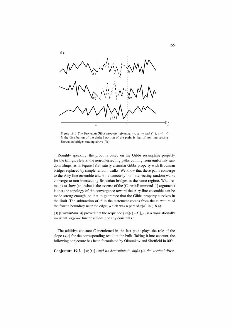
155
x1
x2 y2
y1
f(t)
a b x
t
Figure 19.1 The Brownian Gibbs property: given x1, x2, y1, y2 and f (t), a ≤ t ≤b, the distribution of the dashed portion of the paths is that of non-intersectingBrownian bridges staying above f (t).
Roughly speaking, the proof is based on the Gibbs resampling propertyfor the tilings: clearly, the non-intersecting paths coming from uniformly ran-dom tilings, as in Figure 18.3, satisfy a similar Gibbs property with Brownianbridges replaced by simple random walks. We know that these paths convergeto the Airy line ensemble and simultaneously non-intersecting random walksconverge to non-intersecting Brownian bridges in the same regime. What re-mains to show (and what is the essense of the [CorwinHammond11] argument)is that the topology of the convergence toward the Airy line ensemble can bemade strong enough, so that to guarantee that the Gibbs property survives inthe limit. The subtraction of t2 in the statement comes from the curvature ofthe frozen boundary near the edge, which was a part of x(n) in (18.4).
(3) [CorwinSun14] proved that the sequence Ai(t)+Ci≥1 is a translationallyinvariant, ergodic line ensemble, for any constant C.
The additive constant C mentioned in the last point plays the role of theslope (s, t) for the corresponding result at the bulk. Taking it into account, thefollowing conjecture has been formulated by Okounkov and Sheffield in 00’s:
Conjecture 19.2. Ai(t)i and its deterministic shifts (in the vertical direc-
156 Lecture 19: Airy line ensemble, GUE-corners, and others
tion) are the unique translation–invariant, ergodic line ensembles such thatthe sequence 1√
2(Ai(t)− t2)i≥1 has the Brownian Gibbs property.
Conceptual conclusion. The Airy line ensemble should appear whenever wedeal with a scaling limit of random ensembles of non-intersecting paths at thepoints where their density is low.
19.2 Local limits at special points of the frozen boundary
In the previous lecture we saw the appearance of the Airy line ensemble at ageneric point where the frozen boundary is smooth. However, as we tile vari-ous complicated polygons, the frozen boundary develops various singularities,where the asymptotic behavior changes.
• One type of special points of the boundary arises in any polygons. These arethe points, where the frozen boundary is tangent to a side of the polygon.For instance, in the hexagon we have six such points. In this situation thecorrect scaling factor in the tangential direction to the frozen boundary isL1/2 (where L is the linear size of the domain) and we do not need anyrescaling in the normal direction. The limiting object GUE–corners processconnects us to the random matrix theory and we are going to discuss it inthe next section and continue in the next lecture.
• The frozen boundary can develop cusp singularities. For instance, they arevisible in the connected component of the boundary surrounding the hole inour running example of the holey hexagon, see Figure 24.2 in Lecture 1 andFigures 24.1, 24.5 in Lecture 24. There are two types of these cusps: onetype is presented by two vertical cusps in the above figure, which separatetwo types of frozen regions; the limit shape develops a corner at such cusp.In this situation the scaling factors are L1/3 in the direction of cusp and finitein the orthogonal direction. The scaling limit is known as Cusp–Airy pro-cess, see [OkounkovReshetikhin06], [DuseJohanssonMetcalfe15]. We alsoobserve two cusps of another type in the picture: these cusps are adjacent toa single type of the frozen region each; the limit shape is C1–smooth nearthese cusps. The fluctuations of the discrete boundaries of such cusp are oforder L1/4 and one needs to travel the distance of order L1/2 along the cuspto see a non-trivial 2d picture. The limit is known as the (extended) Pearceyprocess, see [OkounkovReshetikhin05, BorodinKuan08] for its appearancesin tilings.
• Another possible situation is when the frozen boundary (locally near apoint) has two connected components, which barely touch each other.
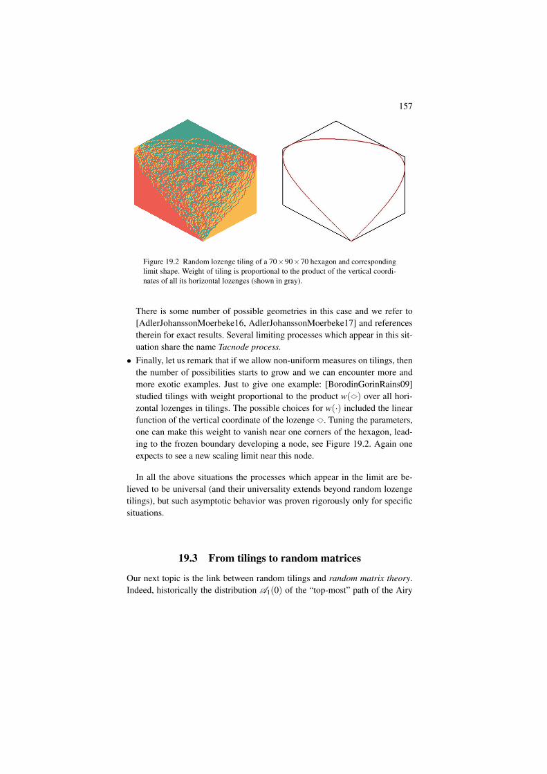
157
Figure 19.2 Random lozenge tiling of a 70×90×70 hexagon and correspondinglimit shape. Weight of tiling is proportional to the product of the vertical coordi-nates of all its horizontal lozenges (shown in gray).
There is some number of possible geometries in this case and we refer to[AdlerJohanssonMoerbeke16, AdlerJohanssonMoerbeke17] and referencestherein for exact results. Several limiting processes which appear in this sit-uation share the name Tacnode process.
• Finally, let us remark that if we allow non-uniform measures on tilings, thenthe number of possibilities starts to grow and we can encounter more andmore exotic examples. Just to give one example: [BorodinGorinRains09]studied tilings with weight proportional to the product w( ) over all hori-zontal lozenges in tilings. The possible choices for w(·) included the linearfunction of the vertical coordinate of the lozenge . Tuning the parameters,one can make this weight to vanish near one corners of the hexagon, lead-ing to the frozen boundary developing a node, see Figure 19.2. Again oneexpects to see a new scaling limit near this node.
In all the above situations the processes which appear in the limit are be-lieved to be universal (and their universality extends beyond random lozengetilings), but such asymptotic behavior was proven rigorously only for specificsituations.
19.3 From tilings to random matrices
Our next topic is the link between random tilings and random matrix theory.Indeed, historically the distribution A1(0) of the “top-most” path of the Airy
158 Lecture 19: Airy line ensemble, GUE-corners, and others
line ensemble at time t = 0, known as the Tracy-Widom distribution, first ap-peared in the random matrix theory. At this point, one might be wondering,what do tilings have in common with matrices and why do the same limitingobjects appear in both topics and we are going to explain that.
The general philosophy comes from the notion of semiclassical limit in rep-resentation theory: large representations of a Lie group G behave like orbits ofthe coadjoint action on the corresponding Lie algebra g.
When G = U(N), the Lie algebra is g = iHerm(N) ∼= Herm(N) (the latteris the space of complex Hermitian matrices). We care about this case, becausetilings in the hexagonal lattice are linked to the representation theory of U(N).This is illustrated by the following proposition, which claims that the numberof tilings of certain domain can be calculated via Weyl’s formula for dimen-sions of U(N) irreducible representations.
Proposition 19.3. The number of tilings of the trapezoid with teeth at positionst1 < t2 < · · ·< tN , as in Figures 14.1, 14.2, is
∏1≤i< j≤N
t j− tij− i
and coincides with the dimension of the irreducible representation of U(N)
with highest weight λ1 ≥ λ2 ≥ ·· · ≥ λN such that tN+1−i = λi +N − i, i =1, . . . ,N.
Proof This is left as an exercise, we only mention three possible approaches:
• One can identify the terms in the combinatorial formula for the expansionof Schur polynomials sλ (x1,x2, . . . ,xN) into monomials with tilings of thetrapezoid. Then use known formulas for evaluations of Schur polynomialssλ (1,1, . . . ,1). We refer to [Macdonald95, Chapter I] for the extensive infor-mation on the Schur polynomials and to [BorodinPetrov13, Section 2.2] forthe review of the interplay between tilings and symmetric polynomials. Thisinterplay appears again in Lecture 22 and is explained there in more details.
• Identify tilings of the trapezoid with basis elements of the irreducible rep-resentation Vλ of U(N) associated to λ . Then use Weyl’s formula to findthe dimension of the irreducible representation of U(N) corresponding to λ .See, e.g., [BorodinPetrov13, Section 2.2] for more details on this approachand further references.
• Identify tilings of the trapezoid with families of non-intersecting paths as inthe previous lecture. Then use LGV theorem from Lecture 2 to count thenumber of such non-intersecting paths via determinants, and use the evalu-ation formulas from [Krattenthaler99] to compute these determinants.
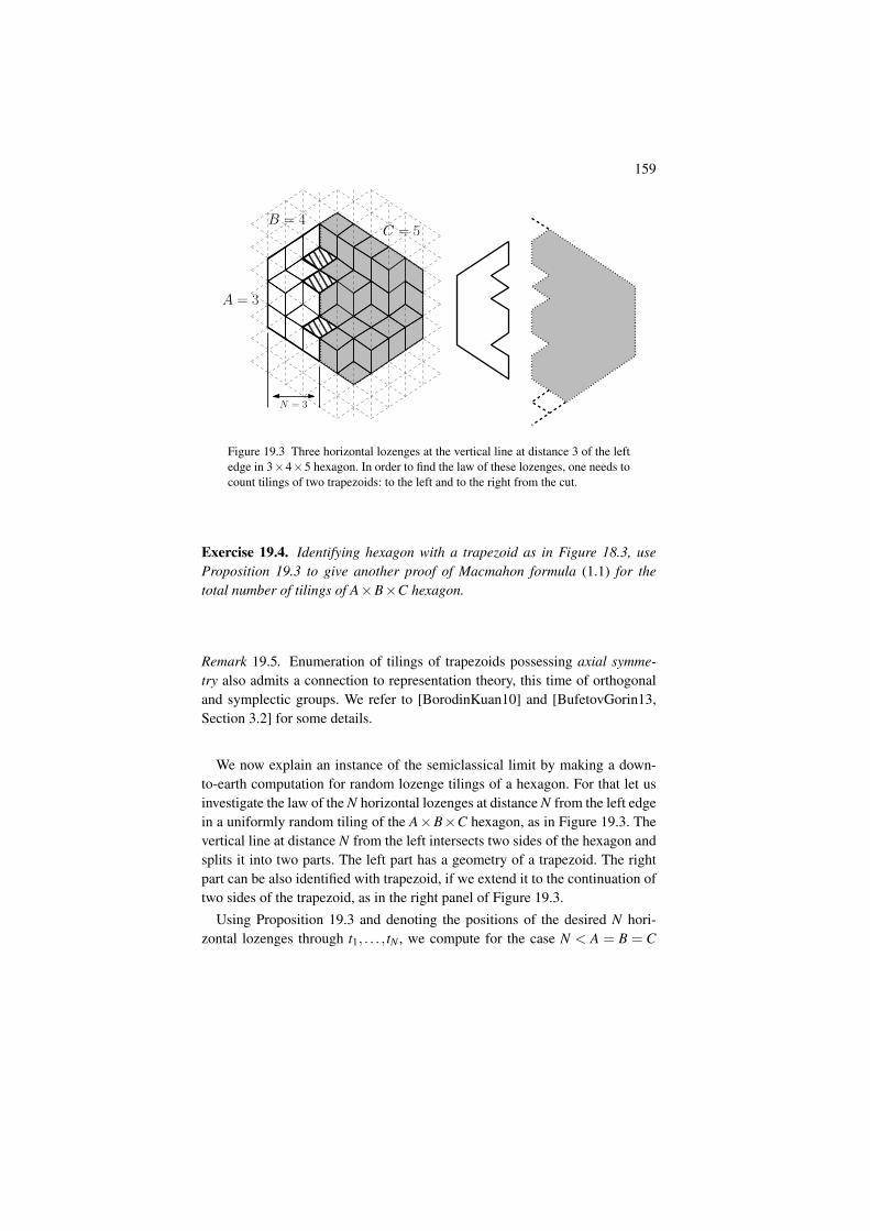
159
N = 3
A = 3
B = 4C = 5
Figure 19.3 Three horizontal lozenges at the vertical line at distance 3 of the leftedge in 3×4×5 hexagon. In order to find the law of these lozenges, one needs tocount tilings of two trapezoids: to the left and to the right from the cut.
Exercise 19.4. Identifying hexagon with a trapezoid as in Figure 18.3, useProposition 19.3 to give another proof of Macmahon formula (1.1) for thetotal number of tilings of A×B×C hexagon.
Remark 19.5. Enumeration of tilings of trapezoids possessing axial symme-try also admits a connection to representation theory, this time of orthogonaland symplectic groups. We refer to [BorodinKuan10] and [BufetovGorin13,Section 3.2] for some details.
We now explain an instance of the semiclassical limit by making a down-to-earth computation for random lozenge tilings of a hexagon. For that let usinvestigate the law of the N horizontal lozenges at distance N from the left edgein a uniformly random tiling of the A×B×C hexagon, as in Figure 19.3. Thevertical line at distance N from the left intersects two sides of the hexagon andsplits it into two parts. The left part has a geometry of a trapezoid. The rightpart can be also identified with trapezoid, if we extend it to the continuation oftwo sides of the trapezoid, as in the right panel of Figure 19.3.
Using Proposition 19.3 and denoting the positions of the desired N hori-zontal lozenges through t1, . . . , tN , we compute for the case N < A = B = C
160 Lecture 19: Airy line ensemble, GUE-corners, and others
(general case can be obtained similarly)
Prob(t1, . . . , tN) =#tilings of left trapezoid×#tilings of right trapezoid
#tilings of the hexagon
∝ ∏1≤i< j≤N
(t j− ti) · ∏1≤a<b≤2A−N
(tb− ta)
∝ ∏1≤i< j≤N
(t j− ti)2 ·N
∏i=1
(ti +1)A−N(A+N− ti)A−N . (19.1)
(Recall the Pochhammer symbol notation: (x)n := x(x+ 1) · · ·(x+ n− 1) =Γ(x+n)/Γ(x).)
Above, 0 ≤ t1 < · · · < tN ≤ A+N − 1 are the positions of the horizontallozenges at level N. Equivalently, they are the teeth of the left trapezoid. Onthe other hand, t1 < t2 < .. . < t2A−N are the positions of the teeth of the righttrapezoid. That is, t1, . . . , tA−N = −1, . . . ,−(A−N), tA+1, . . . , t2A−N =A+N, . . . ,2A−1 and tA−N+1, . . . , tA= t1, . . . , tN.
Exercise 19.6. Generalize the computation (19.1) to arbitrary A× B×Chexagons and arbitrary values of 0≤ N ≤ B+C.
Exercise 19.7. Find an analogue of (19.1) for qVolume–weighted lozenge tilingsof the hexagon.1
We would like to study the limit A→ ∞ of the distribution (19.1), whilekeeping N fixed. It is clear that E[ti] ≈ A/2 when A is large compared to N,because of the symmetry of the model. Hence, recentering by A
2 is necessary.Let us guess the magnitude of the fluctuations by looking at the simplest N = 1case. From (19.1), we have Prob(t) ∝ (t +1)A−1(A+1− t)A−1, which is pro-portional to the product of two binomial coefficients. Recall the De Moivre–Laplace Centra Limit Theorem theorem, which says that if Prob(t) was pro-portional to a single binomial coefficient, then the order of the fluctuations, asA→ ∞, would be
√A. It turns out that the same is true in our case of the prod-
uct of two binomial coefficients. Thus we expect to see a non-trivial scalinglimit in the following regime:
ti =A2+√
Axi, i = 1, . . . ,N. (19.2)
We plug (19.2) into (19.1) and send A→ ∞. With (19.2), we have
∏1≤i< j≤N
(ti− t j)2
∝ ∏1≤i< j≤N
(xi− x j)2, (19.3)
1 The computation is possible for more complicated distributions on tilings as well. Inparticular, [BorodinGorinRains09, Section 10] studies the situation when weights of lozengesare given by elliptic functions in their coordinates.
161
where the hidden constant is independent of the xi’s. Moreover,
(ti +1)A−N(A+N− ti)A−N =(ti +A−N)!
ti!(2A− ti−1)!
(A+N− ti−1)!
=
(3A2 −N +
√Axi
)!(
A2 +√
Axi
)!
(3A2 −√
Axi−1)
!(A2 +N−
√Axi−1
)!.
We can use Stirling’s formula M! =√
2πM(M/e)M(1+o(1)), M→ ∞, in theformula above. It is safe to ignore N and other finite order constants for thecomputation, as only growing terms will give a non-trivial contribution. Usingthe asymptotic expansion ln(1+ x) = x− x2/2+O(x3), x→ 0, we get
(ti +1)A−N(A+N− ti)A−N
≈exp((
3A2 +√
Axi
)(ln(
3A2 +√
Axi
)−1)+(
3A2 −√
Axi
)(ln(
3A2 −√
Axi
)−1))
exp(−(
A2 +√
Axi
)(ln(
A2+√
Axi
)−1)−(
A2 −√
Axi
)(ln(
A2 −√
Axi
)−1))
≈exp(
A[(
32 +
xi√A
)(ln(
1+ 2xi
3√
A
))+
(32 −
xi√A
)ln(
1− 2xi
3√
A
)])exp(
A[−(
12+ xi√
A
)(ln(
1+ 2xi√A
))−(
12 −
xi√A
)ln(
1− 2xi√A
)])≈exp
(−4
3x2
i
).
As a result, in the regime (19.2), we haveN
∏i=1
(ti +1)A−N(A+N− ti)A−N =N
∏i=1
exp(−4
3x2
i
)· (1+o(1)). (19.4)
From (19.1), (19.3), and (19.4), we get the following proposition, whoseproof first appeared in [Nordenstam09].
Proposition 19.8. Consider uniformly random tilings of A×A×A hexagonand let t1, . . . , tN denote the (random) coordinates of N lozenges on the verticalline at distance N from the left edge. The N–dimensional vectors ti− A
2√3A8
1≤i≤N
converge in distribution to the absolutely continuous probability measure on(x1, . . . ,xN) ∈ RN : x1 ≤ ·· · ≤ xN with density proportional to
∏1≤i< j≤N
(xi− x j)2
N
∏i=1
exp(−x2
i2
). (19.5)
162 Lecture 19: Airy line ensemble, GUE-corners, and others
We can go further and look not only at level N (at distance N from the base),but at the first N levels simultaneously. In the tilings model, let t j = (t j
1 < · · ·<t j
j ) be the positions of horizontal lozenges at the j-th level, counted so that we
have 0 ≤ t j1 < · · · < t j
j ≤ A+ j− 1. The combinatorics of tilings implies thatthe interlacing2 inequalities
t j+1i+1 > t j
i ≥ t j+1i , for all relevant i, j.
Proposition 19.9. The N(N +1)/2–dimensional vectors t ji −
A2√
3A8
1≤i≤ j≤N
(19.6)
converge in distribution as A→ ∞ to the absolutely continuous probabilitymeasure on
(x ji )1≤i≤ j≤N ∈ RN(N+1)/2 : x j+1
i+1 ≥ x ji ≥ x j+1
i for all relevant i, j
with density proportional to
∏1≤i< j≤N
(xNj − xN
i ) ·N
∏i=1
exp(−(xN
i )2
2
). (19.7)
Proof We set
t ji =
A2+
√3A8
x ji .
From Proposition 19.8, the law of tNi −
A2√
3A8
1≤i≤N
(19.8)
as A→ ∞ has density proportional to
∏1≤i< j≤N
(xNj − xN
i )2 ·
N
∏i=1
exp(−(xN
i )2
2
)· (1+o(1)), A→ ∞.
By the Gibbs property (following from the uniformity of random tilings), thelaw of the N(N +1)/2–dimensional vectors (19.6) is obtained from the law oftN1 < · · · < tN
N dividing by the number of lozenge tilings of the trapezoid withteeth at the positions tN
i . Therefore, by Proposition 19.3, we need to multiply
2 An interlacing triangular array of integers (or, sometimes, reals) satisfying such inequalities isoften called a Gelfand–Tsetlin pattern. The name originates from the labeling with suchpatterns of the Gelfand–Tsetlin basis in irreducible representations of unitary groups U(N),first constructed in [GelfandTsetlin50].
163
the law of the rescaled vector (19.8) by a constant (independent of the tNi )
multiple of1
∏1≤i< j≤N (tNj − tN
i )∝
1∏1≤i< j≤N (xN
j − xNi )
.
The result follows.
So far, we have only discussed random tilings of hexagons and a scalinglimit of their marginals. What is the relation with random matrices, that wepromised? In the next lecture we are going to show that the distribution (19.7)has random matrix origin: its name is GUE–corners process and it appears inthe celebrated Gaussian Unitary Ensemble.
Lecture 20: GUE–corners process and itsdiscrete analogues.
At the very end of Lecture 19 we obtained an interesting distribution on inter-lacing arrays of reals x j
i 1≤i≤ j≤N as a scaling limit for positions of lozenges inuniformly random tilings of the hexagon near one of the sides of the hexagon.Our next task is to identify this distribution with the so–called GUE–cornersprocess.1
20.1 Density of GUE–corners process
For k dimensional real vector u = (u1, . . . ,uk) and (k + 1)–dimensional realvector v = (v1, . . . ,vk+1) we say that u interlaces with v and write u≺ v, if
v1 ≤ u1 ≤ v2 ≤ u2 ≤ ·· · ≤ uk ≤ vk.
Theorem 20.1. Let X be an N×N matrix of i.i.d. complex Gaussian randomvariables of the form N(0,1)+ iN(0,1) and set M = X+X∗
2 to be its Hermitianpart. Define xm
1 ≤ xm2 ≤ ·· · ≤ xm
m to be the eigenvalues of the principal top-leftcorner of M as in Figure 20.1. Then the array xm
i 1≤i≤m≤N has the density(with respect to the N(N+1)/2–dimensional Lebesgue measure) proportionalto
1x1≺x2≺···≺xN ∏1≤i< j≤N
(xNj − xN
i )N
∏i=1
exp(−(xN
i )2
2
). (20.1)
Our proof closely follows the exposition of [Baryshnikov01], [Neretin03].One earlier appearance of such arguments is [GelfandNaimark50, Section 9.3].
1 Other name used in the literature is the GUE–minors process. Since, by the definition a minoris the determinant of a submatrix (rather than the submatrix itself appearing in the definitionof our process), we choose to use the name GUE–corners instead.
164
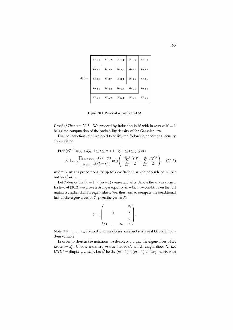
165
Figure 20.1 Principal submatrices of M.
Proof of Theorem 20.1 We proceed by induction in N with base case N = 1being the computation of the probability density of the Gaussian law.
For the induction step, we need to verify the following conditional densitycomputation
Prob(xm+1
i = yi +dyi, 1≤ i≤ m+1 | x ji ,1≤ i≤ j ≤ m
)?∼ 1xm≺y
∏1≤i< j≤m+1(y j− yi)
∏1≤i< j≤m(xmj − xm
i )exp
(−
m+1
∑i=1
(yi)2
2+
m
∑i=1
(xmi )
2
2
), (20.2)
where ∼ means proportionality up to a coefficient, which depends on m, butnot on x j
i or yi.Let Y denote the (m+1)×(m+1) corner and let X denote the m×m corner.
Instead of (20.2) we prove a stronger equality, in which we condition on the fullmatrix X , rather than its eigenvalues. We, thus, aim to compute the conditionallaw of the eigenvalues of Y given the corner X :
Y =
u1
X...
um
u1 . . . um v
.
Note that u1, . . . ,um are i.i.d. complex Gaussians and v is a real Gaussian ran-dom variable.
In order to shorten the notations we denote x1, . . . ,xm the eigenvalues of X ,i.e. xi := xm
i . Choose a unitary m×m matrix U , which diagonalizes X , i.e.UXU∗ = diag(x1, . . . ,xm). Let U be the (m+1)× (m+1) unitary matrix with
166 Lecture 20: GUE–corners process and its discrete analogues.
m×m corner U , the unit diagonal element Um+1,m+1 = 1 and vanishing re-maining elements Um+1,i =Ui,m+1 = 0, 1≤ i≤ m. Set Y = UYU∗, so that
Y =
x1 u′1
. . ....
xm u′mu′1 . . . u′m v′
.
We claim that u′1, . . . ,u′m are still i.i.d. Gaussians and v′ is still a real Gaus-
sian random variable. Indeed, the law of these random variables is obtainedby rotating a Gaussian vector with (independent from it) unitary matrix, whichkeeps the distribution unchanged.
Since conjugation of Y does not change its eigenvalues, it remains to com-pute the law of the eigenvalues of Y . For that we evaluate the characteristicpolynomial of Y . Expanding the determinant by the last column, we get
det(y · Id− Y
)=
m
∏i=1
(y− xi) ·
(y− v′−
m
∑i=1
|u′i|2
y− xi
). (20.3)
Let us denote |u′i|2 through ξi. Since u′i is a two-dimensional Gaussian vectorwith independent N(0,1/2) components, ξi has standard exponential distribu-tion of density exp(−ξ ), ξ > 0. Since the characteristic polynomial of Y canbe alternatively computed as ∏
m+1i=1 (y− yi), (20.3) implies
m+1∏i=1
(y− yi)
m∏i=1
(y− xi)= y− v′−
m
∑i=1
ξi
y− xi. (20.4)
Here is a corollary of the last formula.
Lemma 20.2. We have
ξa =−∏
m+1b=1 (xa− yb)
∏1≤c≤m;c6=a(xa− xc), 1≤ a≤ m, and v′ =
m+1
∑b=1
yb−m
∑a=1
xa.
(20.5)
Proof Multiplying (20.4) with y− xa and then setting y = xa, we get the for-mula for ξa is obtained. Looking at the coefficient of 1
y in the expansion of(20.4) into a series in 1
y for large y, we get the formula for v′.
In addition we have the following statement, whose proof we leave as anexercise.
167
Exercise 20.3. In formula (20.4) all the numbers ξa, 1 ≤ a ≤ m are non-negative if and only if the sequences xi and yi interlace, i.e.~x≺~y.
We continue the proof of Theorem 20.1. Since we know the joint distributionof ξa and v′, and we know their link to yi through (20.4), it only remainsto figure out the Jacobian of the change of variables ξa, 1 ≤ a ≤ m; v′ 7→yi, 1≤ i≤m+1. Straightforward computation based on Lemma 20.2 showsthat
∂ξa
∂yb= ξa ·
1xa− yb
,∂v′
∂yb= 1.
Hence, the desired Jacobian is
ξ1 · · ·ξm ·det
11
xa−yb
...1
. (20.6)
We can simplify the last formula using the following determinant computation.
Lemma 20.4 (Cauchy determinant formula). For any u1, . . . ,uN , v1, . . . ,vN wehave
det(
1ua− vb
)N
a,b=1=
∏a<a′(ua−ua′)∏b<b′(vb− vb′)
∏Na,b=1(ua− vb)
(20.7)
Proof Multiply (20.7) by ∏Na,b=1(ua− vb) and notice that the left-hand side
becomes a polynomial in ui and v j of degree N(N − 1). This polynomial isskew symmetric both in variables (u1, . . . ,uN) and in variables (v1, . . . ,vN).Therefore, it has to be divisible by ∏a<a′(ua− ua′)∏b<b′(vb− vb′). Compar-ing the degrees, we conclude that (20.7) has to hold up to multiplication by aconstant. Comparing the coefficients of the leading monomials we see that thisconstant is 1.
Sending one of the variables in (20.7) to infinity, we compute the determi-nant in (20.6). Hence, the desired Jacobian is
ξ1 · · ·ξm ·∏
1≤a<a′≤m(xa− xa′) ∏
1≤b<b′≤m+1(yb− yb′)
m∏
a=1
m+1∏
b=1(xa− yb)
=
∏1≤b<b′≤m+1
(yb− yb′)
∏1≤a<a′≤m
(xa− xa′).
Using the explicit formula for the joint density of ξa, 1 ≤ a ≤ m; v′, weconclude that the conditional density of y1, . . . ,ym+1 given x1, . . . ,xm is propor-
168 Lecture 20: GUE–corners process and its discrete analogues.
tional to∏
1≤b<b′≤m+1(yb− yb′)
∏1≤a<a′≤m
(xa− xa′)exp
(−
m
∑a=1
ξa−(v′)2
2
).
Inserting the indicator function from Exercise 20.3 into the last formula we get(20.2), as soon as we notice that the definition of the matrix Y implies
m
∑a=1
ξa+(v′)2
2=
12
(Trace(Y 2)−
m
∑a=1
(xa)2
)=
12
(m+1
∑b=1
(yb)2−
m
∑a=1
(xa)2
).
Exercise 20.5. Repeat the argument for real (rather than complex) matrix Xwith i.i.d. N(0,1) matrix elements.2 How does the density (20.1) change?
20.2 GUE–corners process as a universal limit
In Lecture 19 we obtained GUE–corners process as a scaling limit for randomlozenge tilings of hexagons. Conjecturally, it appears much wider.
Conjecture 20.6 ([OkounkovReshetikhin06]). GUE–corners process is a uni-versal scaling limit for uniformly random lozenge tilings at the points wherethe boundary of the frozen boundary of a tiling is tangent to a straight segmentof the boundary of the tiled domain.
For trapezoid domains Conjecture 20.6 was settled in [GorinPanova13]. Formore general domains it is still open.
Similarly to the extended sine process (or ergodic Gibbs translationally in-variant measure), which we saw in the bulk of the tilings, and the extended Airyprocess (or Airy line ensemble) which appears at the edges of liquid regions,the GUE–corners process can be obtained as a solution to a certain classifi-cation problem. That was an argument of [OkounkovReshetikhin06] for thevalidity of Conjecture 20.6. The classification problem in which GUE–cornersprocess appears can be linked to the representation theory and to the ergodictheory and we now present it.
Let U(N) denote the group of all (complex) N×N unitary matrices. Thereis a natural embedding of U(N) into U(N + 1) identifying an operator in Ndimensional space with a one in N +1 dimensional space fixing the last basis
2 In this case M = X+X∗2 is known as the Gaussian Orthogonal Ensemble.
169
vector. Through these embeddings we can define the infinite-dimensional uni-tary group as the union of all finite dimensional groups: U(∞) =
⋃∞N=1 U(N).
Each element of U(∞) is an infinite matrix, whose upper–left k× k corner isa unitary matrix of size k and the rest of the matrix is filled with 1’s on thediagonal and with 0’s everywhere else.
Consider the space H of all infinite complex Hermitian matrices. Theirmatrix elements hi j ∈C, i, j = 1,2,3, . . . satisfy hi j = h ji. The group U(∞) actson H by conjugations and we can study U(∞)–invariant probability measureson H . We call such measure ergodic if it is an extreme point of the convex setof all U(∞)–invariant probability measures.
One can construct three basic examples of ergodic measures or, equivalently,infinite random Hermitian matrices:
1 A deterministic diagonal matrix γ1 · Id, γ1 ∈ R.2 Gaussian Unitary Ensemble. Take γ2 ∈ R>0 and an infinite matrix X of
i.i.d. N(0,1)+ iN(0,1) matrix elements. Consider a random matrix γ2X+X∗
2 .3 Wishart (or Laguerre) ensemble. Take α ∈ R and an infinite vector V
of i.i.d. N(0,1) + iN(0,1) components. Consider a rank 1 random matrixαVV ∗.
A theorem of Pickrell and Olshanski-Vershik claims that sums of indepen-dent matrices from these three ensembles exhaust the list of ergodic U(∞)–invariant measures.
Theorem 20.7 ([Pickrell91], [OlshanskiVershik96]). Ergodic U(∞)–invariantmeasures on H are parameterized by γ1 ∈ R, γ2 ∈ R≥0, and a collection ofreal numbers αi, such that ∑i α2
i < ∞. The corresponding random matrix isgiven by
γ1 · Id+ γ2X +X∗
2+∑
iαi
(ViV ∗i
2− Id
), (20.8)
where all terms are taken to be independent.
Note that, in principle, the subtraction of ∑i αiId could have been absorbedinto the γ1 term. However, in this case the sum over i would have failed toconverge (on the diagonal) for sequences αi such that ∑i α2
i < ∞, but ∑i |αi|=∞.
One sees that the GUE–corners process appears in a particular instance ofTheorem 20.7 with γ1 = 0 and αi = 0. Let us explain how to link this appear-ance to the limits of random tilings.
170 Lecture 20: GUE–corners process and its discrete analogues.
Lemma 20.8. Let M ∈ H be a random U(∞)–invariant infinite hermitianmatrix and denote mN
1 ≤mN2 ≤ ·· · ≤mN
N the eigenvalues of its principle N×Ntop-left corner. Then the eigenvalues m j
i interlace, which means
mN+1i ≤ mN
i ≤ mN+1i+1 , 1≤ i≤ N.
Moreover, they satisfy the Gibbs property, which says that conditionally on thevalues of mN
1 ,mN2 , . . . ,m
NN , the N(N− 1) eigenvalues m j
i , 1 ≤ i ≤ j < N, haveuniform distribution on the polytope determined by the interlacing conditions.
Sketch of the proof The interlacement is a general linear algebra fact abouteigenvalues of corners of a hermitian matrix. The conditional uniformity canbe proven by a version of the argument that we used in determining the densityof GUE–corners process in Theorem 20.1.
In fact, one can show that classification of ergodic U(∞)–invariant randomhermitian matrices of Theorem 20.7 is equivalent to the classification of allergodic Gibbs measures on infinite arrays mi
j of interlacing real numbers.
Lemma 20.8 explains why we expect the scaling limit of uniform measureon tilings near a straight boundary of the domain to be one of the measuresin Theorem 20.1: horizontal lozenges in tiling near the boundary satisfy thediscrete versions of the interlacement and Gibbs property. Hence, we expectcontinuous analogues to hold for the limiting object. But why do we observeonly the GUE–corners process, but no deterministic or Wishart components?
This can be explained by very different Law of Large Numbers for these en-sembles. Take a random infinite hermitian matrix M and consider the empiricalmeasure of the eigenvalues of its corner:
δN =
1N
N
∑i=1
δmiN.
The N → ∞ behavior of the empirical measure is very different for the threebasic examples:
1 For the diagonal matrix γ1 · Id, δ N is a unit mass at γ1 for all N.2 For the GUE ensemble with γ2 = 1, the eigenvalues as N → ∞ fill the seg-
ment [−2√
N,2√
N], after normalization by√
N, the measure δ N convergesto the Wigner semicircle law.
3 For the rank 1 Wishart matrix 12VV ∗, the empirical measures δ N has mass
N−1N at 0 with an outlier of mass 1
N at point ≈ N as N→ ∞.
Exercise 20.9. Prove the last statement about rank 1 Wishart matrices.
171
On the other hand, in the tilings picture, we deal with a point where thefrozen boundary is tangent to the straight boundary of the domain. Hence, thefrozen boundary locally looks like a parabola, which is consistent only with[−2√
N,2√
N] segment filled with eigenvalues in the GUE case.
Conceptual conclusion. The GUE–corners process is expected appear in thescaling limit near the frozen boundary tangency points whenever we deal withinterlacing triangular arrays of particles satisfying (asymptotically) conditionaluniformity.
This prediction matches rigorous results going beyond random tilings. Forinstance, [GorinPanova13, Gorin13, Dimitrov16] demonstrated the appearanceof the GUE–corners process as the scaling limit of the six-vertex model.
20.3 A link to asymptotic representation theory andanalysis
In Theorem 20.7 and Lemma 20.8 we saw how GUE–corners process getslinked to the classification problem of ergodic theory or asymptotic represen-tation theory. But in fact, the same connection exists already on the discretelevel of random lozenge tilings.
Let us present a discrete space analogue of Theorem 20.7. For that we let T
denote the set of all lozenge tilings of the (right) half–plane, such that far upthere are only lozenges of type and far down there are only lozenges of type
, cf. Figure 20.2. This constraint implies that there is precisely one horizontallozenge on the first vertical line, precisely two on the second one, preciselythree on the third one, etc. Their coordinates interlace, as in Sections 10.3or in Proposition 19.9. When one forgets about tilings considering only thesecoordinates, then the resulting object is usually called an (infinite) Gelfand–Tsetlin pattern or a path in the Gelfand–Tsetlin graph.
We aim to study the probability measures on T , which are Gibbs in thesame sense as in Definition 13.4 of Lecture 13. Due to our choice of boundaryconditions, the interlacing can be equivalently restated in terms of horizontallozenges : given the positions of N horizontal lozenges on Nth vertical, theconditional distribution of N(N− 1)/2 horizontal lozenges on the first N− 1verticals is uniform on the set defined by the interlacing conditions.
Theorem 20.10 ([AissenSchoenbergWhitney52], [Edrei53, Voiculescu76,VershikKerov82, BorodinOlshanski12, Petrov12c, GorinPanova13]). The er-godic Gibbs measures on T are parameterized by two reals γ+ ≥ 0, γ− ≥ 0
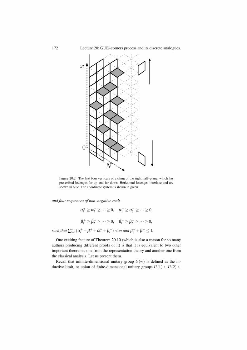
172 Lecture 20: GUE–corners process and its discrete analogues.
0
N
x
Figure 20.2 The first four verticals of a tiling of the right half–plane, which hasprescribed lozenges far up and far down. Horizontal lozenges interlace and areshown in blue. The coordinate system is shown in green.
and four sequences of non–negative reals
α+1 ≥ α
+2 ≥ ·· · ≥ 0, α
−1 ≥ α
−2 ≥ ·· · ≥ 0,
β+1 ≥ β
+2 ≥ ·· · ≥ 0, β
−1 ≥ β
−2 ≥ ·· · ≥ 0,
such that ∑∞i=1(α
+i +β
+i +α
−i +β
−i )< ∞ and β
+1 +β
−1 ≤ 1.
One exciting feature of Theorem 20.10 (which is also a reason for so manyauthors producing different proofs of it) is that it is equivalent to two otherimportant theorems, one from the representation theory and another one fromthe classical analysis. Let us present them.
Recall that infinite-dimensional unitary group U(∞) is defined as the in-ductive limit, or union of finite-dimensional unitary groups U(1) ⊂ U(2) ⊂
173
U(3) ⊂ ·· · ⊂U(∞). A (normalized) character χ(u) of U(∞) is a continuouscomplex function on the group, which is:
1 central, i.e. χ(ab) = χ(ba) for all a,b ∈U(∞),2 positive–definite, i.e. for each k = 1,2, . . . , complex numbers z1, . . . ,zk and
elements of the group u1, . . . ,uk we have
k
∑i, j=1
ziz jχ(uiu−1j )≥ 0,
3 Normalized, i.e. χ(e) = 1, where e is the unit element (diagonal matrix of1s) in U(∞).
The characters of U(∞) form a convex set, i.e. the convex linear combinationof characters is again a character, and we are interested in extreme ones, whichcan not be decomposed into linear combination of others. As it turns out, thecomplete list of extreme characters is given by Theorem 20.10. The value ofan extreme character corresponding to the parameters of Theorem 20.10 on thematrix U ∈U(∞) is given by
χ(U) = ∏u∈Spectrum(U)
eγ+(u−1)+γ−(u−1−1)∞
∏i=1
1+β+i (u−1)
1−α+i (u−1)
1+β−i (u−1−1)
1−α−i (u−1−1)
,
(20.9)Note that all but finitely many eigenvalues of a matrix U ∈U(∞) are equal to1, therefore, the product over u in (20.9) is actually finite. The double multi-plicativity (in u and in i) of the extreme characters is a remarkable feature ofU(∞), which has analogues for other infinite–dimensional groups. However,nothing like this is true for the finite–dimensional unitary groups U(N), whoseextreme characters are much more complicated (normalized) Schur polynomi-als sλ (u1, . . . ,uN).
The correspondence between Theorem 20.10 and characters of U(∞) goesthrough the expansion of the restrictions of characters. Take any character χ ofU(∞) and consider its restriction to U(N). This restriction is a symmetric func-tion in N eigenvalues u1, . . . ,uN of N×N unitary matrix and can be expandedin Schur polynomials basis as follows:
χ∣∣U(N)
(u1, . . . ,uN) = ∑λ=(λ1≥λ2≥···≥λN)∈ZN
PN(λ )sλ (u1, . . . ,uN)
sλ (1, . . . ,1). (20.10)
One proves that the coefficients PN(λ ) are non–negative and sum up to 1: thefirst condition follows from positive-definiteness and the second one is impliedby the normalization χ(e) = 1. By setting µi = λi +N− i, these coefficientsthus define a probability distribution on N tuples of horizontal lozenges as at
174 Lecture 20: GUE–corners process and its discrete analogues.
the Nth vertical line of the lozenge tiling of the right halfplane, cf. Figure 20.2.With a bit more work one proves that the correspondence χ↔P1,P2,P3, . . .of (20.10) is a bijection between characters of U(∞) and Gibbs measures onT .
For another equivalent form of Theorem 20.10 consider a doubly–infinitesequence of reals . . .d−2,d−1,d0,d1,d2, . . . and introduce a doubly–infiniteToeplitz matrix D by D[i, j] = d j−i, i, j = . . . ,−1,0,1, . . . . The matrix D iscalled totally–positive, if all (finite) minors of D are non–negative. For a nor-malization, we further assume that the sum of elements in each row of D is 1,i.e. ∑
∞i=−∞ di = 1 3. Then the classification of totally positive doubly–infinite
Toeplitz matrices is equivalent to Theorem 20.10, with bijection given by thegenerating series (convergent for u in the unit circle on complex plane):
∞
∑i=−∞
uidi = eγ+(u−1)+γ−(u−1−1)∞
∏i=1
1+β+i (u−1)
1−α+i (u−1)
1+β−i (u−1−1)
1−α−i (u−1−1)
.
The classification of totally–positive Toeplitz matrices was originally moti-vated by a data smoothing problem. Suppose that we have a real data sequencexi, i∈Z and a pattern di, i∈Z, then we can construct a smoothed data sequenceyi through
yi = ∑j
xi− jd j.
One shows that the amount of sign–changes (“oscillations”) in yi is alwayssmaller than that in xi if and only if the corresponding Toeplitz matrix D[i, j] =d j−i is totally–positive.
The reason why Theorem 20.10 is linked to totally positive Toeplitz matriceslies in the formulas for the coefficients in the decomposition (20.10). From oneside, they must be non–negative, as they define probability measures, on theother hand, they essentially are the minors of a certain Toeplitz matrix, as thefollowing exercise shows:
Exercise 20.11. Consider the following decomposition of symmetric two-sidedpower series in variables u1, . . . ,uN:
N
∏i=1
(∑k∈Z
ck(ui)k
)= ∑
λ=(λ1≥λ2≥···≥λN)∈ZN
cλ ·det[u
λ j+N− ji
]N
i, j=1
∏1≤i< j≤N(ui−u j). (20.11)
Multiplying both sides by the denominator show that the coefficients cλ are
3 A relatively simple argument shows that if D is a totally–positive Toeplitz matrix, then eitherdi =CRi for all i, or replacing di by CRidi with appropriate C and R, we can guarantee thecondition ∑
∞i=−∞ di = 1. Therefore, the normalization condition does not reduce the generality.
175
computed as
cλ = det[cλi−i+ j
]Ni, j=1 .
Using the Weyl character formula (cf. [Weyl39]) one identifies the Schurfunctions sλ (u1, . . . ,uN) with the ratios in the right-hand side of (20.11).Hence, the coefficients cλ of Exercise 20.11 differ from PN(λ ) in (20.10) bythe factor sλ (1, . . . ,1). This factor is a positive integer (it counts the dimensionof a representation of U(N) as well as lozenge tilings of a trapezoid domain,see Proposition 19.3 and Section 22.2) — hence, non-negativity of cλ andPN(λ ) is the same condition.
The character theory for U(∞) also admits a q–deformation, which turns tobe closely related both to the study of qVolume–weighted random tilings and tothe quantum groups, see [Gorin10, GorinOlshanski15, Sato19].
We end this lecture by a remark that both Theorems 20.7 and 20.10, aswell as their q–deformations fit into a general framework for studying Gibbsmeasures on branching graphs. These graphs can be very different and werefer to [Kerov03], [BorodinOlshanski13], [BorodinOlshanski16, Section 7]for some details and examples.
Lecture 21: Discrete log-gases.
21.1 Log-gases and loop equations
Recall that in Lecture 19 we computed in (19.1) the law of horizontal lozengeson N-th vertical of randomly tiled equilateral hexagon with side length A:
P(x1, . . . ,xN) ∝ ∏1≤i< j≤N
(xi− x j)2
N
∏i=1
w(xi), (21.1)
where w(x) = (x+1)A−N(A+N−x)A−N . The distribution of form (21.1) witharbitrary w is usually called “log–gas” in statistical mechanics. The name orig-inates from the traditional rewriting of (21.1) as
exp
(β ∑
1≤i< j≤NH(xi,x j)+
N
∑i=1
lnw(xi)
), H(x,y) = ln |x− y|, β = 2,
(21.2)where H(x,y) represents the functional form of the interaction between parti-cles (which is logarithmic in our case) and β is the strength of interaction.
The distributions of the form (21.2) with xi ∈ R or xi ∈ C are widespreadin the random-matrix theory, where they appear as distributions of eigenval-ues for various ensembles of matrices, see [Forrester10]. In this setting theparameter β is the dimension of the (skew)–field to which the matrix elementsbelong. Here β = 1,2,4 corresponds to reals, complex numbers, and quater-nions, respectively. General real values of parameter β also have relevance intheoretical physics and statistical mechanics, but we are not going to discussthis here.
One powerful tool for the study of log-gases as the number of particles Ngoes to infinity is based on certain exact relations for the expectation of observ-ables1 in the system. The usefulness of these relations was understood by the
1 By an observable we mean a function f (X) of the random system state X , such that theexpectation E f (X) is accessible either through explicit formulas or equations fixing it.
176
177
mathematical community since [Johansson98]; before that they were known totheoretical physicists under the name of loop or Dyson–Schwinger equations;we refer to [Guionnet19] for a recent review.
These equations can be treated as far–reaching generalizations of the follow-ing characterization of the Gaussian law. Let ξ be a standard Normal N(0,1)random variable and let f (x) be a polynomial. Then
E[ξ f (ξ )
]= E
[f ′(ξ )
](21.3)
and the relation (21.3) can be used to compute all the moments Eξ k and, hence,to reconstruct the distribution of ξ .
In a similar spirit the loop equations for (continuous space) log-gases can beobtained by a smart integration by parts and further used to extract probabilisticinformation.
In the context of this book we are interested in the discrete setting whenthe particles xi in (21.1) are constrained to the lattice Z. It took a while togeneralize the loop equations to such setting, since the naive replacement ofintegration by parts with summation by parts did not seem to work. The correctform of equations was recently introduced in [BorodinGorinGuionnet15], itwas guided by the notion of qq–characters of [Nekrasov15].
Theorem 21.1 (Nekrasov equation, discrete loop equation). Consider a pointprocess (x1 < x2 < · · ·< xN)⊂0, . . . ,M with law of the form (21.1). Supposethat there exist functions ϕ+(z),ϕ−(z) such that
1 Functions ϕ+(z) and ϕ−(z) are holomorphic in a complex neighbourhoodof [0,M]
2 For any x ∈ 1, . . . ,M we have
w(x)w(x−1)
=ϕ+(x)ϕ−(x)
.
3 ϕ+(M+1) = ϕ−(0) = 0.
Then the function RN(z) defined by
RN(z) = ϕ−(z)E
N
∏i=1
(1− 1
z− xi
)+ϕ
+(z)EN
∏i=1
(1+
1z− xi−1
)(21.4)
is holomorphic in the neighbourhood of [0,M].
Remark 21.2. The theorem admits a generalization to distributions involvingan additional parameter β similarly to (21.2). However, rather than straight-forward ∏i< j |xi− x j|β one has to use a more delicate deformation involvingGamma-functions, see [BorodinGorinGuionnet15] for the details.
178 Lecture 21: Discrete log-gases.
Proof of Theorem 21.1 Note that RN(z) is a meromorphic function in theneighbourhood of [0,M] with possible poles only at 0,1, . . . ,M + 1. Moreprecisely, the first term of (21.4) might have poles only at z = xi ∈ 0, . . . ,Mand the second term only at z = xi +1 ∈ 1, . . . ,M+1.
Thus, in order to show that RN(z) is holomorphic, it is enough to prove thatRN(z) has no poles at 0, . . . ,M+1. Note that in the point process (x1, . . . ,xN)
all particles are almost surely at distinct positions, hence all poles of RN mustbe simple.
For the point z = 0, we have ϕ−(0) = 0, hence, in the first term of (21.4) apossible simple pole at z = 0 cancels out with the zero of ϕ−, while the secondterm has no pole at 0. Therefore, RN(z) has no pole at 0. Similarly for z=M+1a possible pole in the second term cancels out, while the first term has no poles.Thus, RN(z) has no pole at M+1.
Let m∈ 1, . . . ,M. Since all poles of RN(z) are simple, it is enough to provethat the residue at m vanishes. Residue at m results from configurations withxi = m for some i (first term) or configurations with xi = m+ 1 for some i.Expanding E in (21.4) we get
resmRN = ∑i
res(i)m RN ,
where
res(i)m RN =− ∑~x:xi=m
ϕ−(m)P(~x)∏
j 6=i
(1− 1
m− x j
)+ ∑
~x:xi=m−1ϕ+(m)P(~x)∏
j 6=i
(1+
1m− x j−1
).
Note that we can pair configurations~x in the first term and~x−(i) = (x1, . . . ,xi−1, . . . ,xN) in the second term. The poles cancel out leading to res(i)m RN = 0,once we prove
ϕ−(m)P(x1, . . . ,xi−1,m,xi+1, . . . ,xN)∏
j 6=i
(1− 1
m− x j
)= ϕ
+(m)P(x1, . . . ,xi−1,m−1,xi+1, . . . ,xN)∏j 6=i
(1+
1m− x j−1
). (21.5)
179
The validity of (21.5) can be checked directly using (21.1):
LHS = (−1)i−1ϕ−(m)w(m) ∏
j,k 6=ij<k
(x j− xk)2∏j 6=i
[(m− x j)
2w(x j)m− x j−1
m− x j
]
= (−1)i−1ϕ+(m)w(m−1) ∏
j,k 6=ij<k
(x j− xk)2∏j 6=i
[(m− x j−1)2w(x j)
m− x j
m− x j−1
]
= RHS.
Remark 21.3. For the above cancellation argument we also should check theboundary cases when one of the configurations~x,~x−(i) is not well-defined. Butthe computation above shows that in such cases the corresponding term inres(i)m RN will vanish either due to ∏(xi− x j)
2 in the law or due to the boundarycondition ϕ+(M+1) = ϕ−(0) = 0.
Theorem 21.1 can be used to describe various probabilistic properties of log-gases. In particular, it can be applied to the asymptotic study of the uniformlyrandom lozenge tilings of the hexagon. We are going to show two applications.The first one produces another way (in addition to the approaches of Lectures10 and 16) to compute the limit shape for the tilings and see the frozen bound-ary — inscribed ellipse. The second one (we only sketch the arguments there)leads to the Gaussian Fluctuations, which we already expect to be describedby the Gaussian Free Field after Lectures 11 and 12.
21.2 Law of Large Numbers through loop equations
We start by specializing Theorem 21.1 to the distribution of the lozenges onthe section of hexagon as in (19.1), (21.1).
Note that for w(x) = (x+1)A−N(A+N− x)A−N we have
w(x)w(x−1)
=x+A−N
xA+N− x
2A− x.
Hence we can take
ϕ+(z) = (z+A−N)(A+N− z), ϕ
−(z) = z(2A− z),
180 Lecture 21: Discrete log-gases.
and by Theorem 21.1 the function
RN(Nz)N2 = z
(2AN− z)E
N
∏i=1
(1− 1
N(z− xiN )
)
+
(z+
A−NN
)(A+N
N− z)E
N
∏i=1
(1+
1N(z− xi
N −1N )
)is an entire function. For the limit shape of tilings, we want to consider N→∞
with A = aN for some fixed a. Note that for z away from [0, A+NN ] we have
N
∏i=1
(1− 1
N(z− xiN )
)= exp
(N
∑i=1
ln(
1− 1N(z− xi
N )
))
= exp
(− 1
N ∑i
1z− xi
N+O(1/N)
)→ exp(−G(z)),
where G(z) is the Cauchy–Stieltjes transform
G(z) =ˆ a+1
0
1z− y
µ(dy),
and µ is the limiting density at (1,y) of horizontal lozenges as N→∞. Recallthat the existence of the deterministic µ (or, more generally, the limit shape)was proved earlier using either a concentration of martingales or variationalproblem (see Lectures 5-7).
Repeating the same computation for the second term, for z away from[0, a+1] we have
RN(Nz)N2 −−−→
N→∞R∞(z)= z(2a−z)exp(−G(z))+(z+ a−1)(a+1−z)exp(G(z)).
(21.6)
Proposition 21.4. R∞(z) is an entire function.
Proof Note that outside of [0; a+1] the holomorphicity is immediate. More-over, outside of [0; a+1] entire functions RN(Nz)
N2 converge to R∞(z).Take a closed contour C around [0; a+1]. For any z inside C, Cauchy integral
formula readsRN(Nz)
N2 =1
2πi
˛C
RN(Nv)N2(v− z)
dv.
Taking N→ ∞ we get a holomorphic inside C function
12πi
˛C
R∞(v)(v− z)
dv,
181
which coincides with R∞(z) outside of [0; a+1]. Hence R∞(z) is entire.
Corollary 21.5. R∞(z) is a degree 2 polynomial.
Proof R∞ is an entire function growing as z2 when z→ ∞. Hence R∞ is adegree two polynomial by Liouville’s theorem (by Cauchy’s integral formulathe second derivative is bounded, hence constant).
Let us explicitly compute this degree 2 polynomial. Note that
G(z) =1z+
cz2 + . . . ,
when z→ ∞. Hence, using Taylor expansion for exp, for z→ ∞ we have
R∞(z) = z(2a− z)(1−G(z)+G(z)2
2+o(z−2))
+(z+ a−1)(a+1− z)(1+G(z)+G(z)2
2+o(z−2))
=(−z2 +(2a+1)z+(c−2a− 1
2 ))+(−z2 +(2−1)z+(a2−1− c+2− 1
2 ))
+o(1) =−2z2 +2(a+1)z+ a2−2a+o(1).
But R∞(z) is a polynomial, hence o(1) term is equal to 0 and
R∞(z) =−2z2 +2(a+1)z+ a2−2a.
Comparing the definition (21.6) of R∞ with the expression above, we get aquadratic equation for exp(G(z)), namely
z(2a− z)exp(−G(z))+(z+ a−1)(a+1− z)exp(G(z))
=−2z2 +2(a+1)z+ a2−2a. (21.7)
Solving it, we can get an explicit formula for G(z), which is a Stieltjes trans-form of µ , hence, we can recover µ . Integrating it we get a formula for thelimit shape (asymptotic height function of tilings). Therefore, Theorem 21.1gives one more approach to computing the LLN, with others being the Kenyon-Okounkov theory and steepest descent analysis of the correlation kernel.
Exercise 21.6. For each fixed a the function G(z) found from (21.7) has tworeal branching points (of type
√z; they correspond to the points where the
density of µ reaches 0 or 1). If we start varying a, then these branching pointsform a curve in ( 1
a ,z) plane. Find out how this curve corresponds to the circleinscribed into the unit hexagon.
Hint: Dealing with lozenges along the vertical line at distance 1 from the leftboundary of a× a× a hexagon is essentially the same as dealing with lozengesalong the vertical line at distance 1
a from the left boundary of 1×1×1 hexagon.
182 Lecture 21: Discrete log-gases.
Exercise 21.7. Consider the distribution on 0≤ x1 < x2 < · · ·< xN ≤M withweight proportional to2
∏1≤i< j≤N
(xi− x j)2
N
∏i=1
(Mxi
). (21.8)
Assuming that the Law of Large numbers holds in the system and using discreteloop equations, find explicitly the limit of the empirical measures 1
N ∑Ni=1 δxi/N
as M,N→ ∞ in such a way that MN →m > 1.
21.3 Gaussian fluctuations through loop equations
Our next step is to improve the arguments of the previous section, taking in theconsideration lower order terms of RN(Nz). Eventually this provides access tothe global fluctuations in the system.
We only sketch the approach, for the detailed exposition see[BorodinGorinGuionnet15]. We have
N
∏i=1
(1− 1
N(z− xiN )
)= exp
(N
∑i=1
ln(
1− 1N(z− xi
N )
))
= exp
(−G(z)−∆GN(z)+
12N2
N
∑i=1
1(z− xi
N )2 +O(1/N2)
),
where ∆GN(z) is a random fluctuation of the (empirical) Stieltjes transform:
∆GN(z) =1N
N
∑i=1
1z− xi
N−ˆ
1z− y
µ(dy).
Note that as N→ ∞
12N2
N
∑i=1
1(z− xi
N )2 =− 1
2N2∂
∂ z
(N
∑i=1
1z− xi
N
)=− 1
2NG′(z)+o(1).
Hence,
N
∏i=1
(1− 1
N(z− xiN )
)= exp
(−G(z)−∆GN(z)−
12N
G′(z)+O(1/N2)
).
2 This distribution appears on sections of uniformly random domino tilings of the Aztecdiamond as in Figure 1.10.
183
Making a similar computation for the second term of RN(Nz) we eventuallyget
RN(Nz)N2 = ϕ
−N (Nz)exp(−G(z))+ϕ
+N (Nz)exp(G(z))
+E[∆GN(z)
](−ϕ−N (Nz)exp(−G(z))+ϕ
+N (Nz)exp(G(z))
)+
1N(some explicit function of G(z))+o(1/N), (21.9)
where
ϕ+N (Nz) =
ϕ+(Nz)N2 =
(z+
A−NN
)(A+N
N− z),
ϕ+N (Nz) =
ϕ−(Nz)N2 = z
(2AN− z).
Remark 21.8. We use the lower subscript N in ϕ±N (Nz) to emphasize that
these functions might depend on N for general discrete log-gases. Note thatin the hexagon case with scaling A = aN the functions ϕ
±N (Nz) actually are
N–independent.
Remark 21.9. The identity (21.9), or, more precisely, the o(1/N) part of it,requires an asymptotic estimate of E[∆GN(z)]. It turns out that E[∆GN(z)] =O(1/N), but the proof of this fact is a nontrivial argument based on “self-improving” estimates, see [BorodinGorinGuionnet15] for details.
The identity (21.9) has the form
RN(Nz)N2 = R∞(z)+E
[∆GN(z)
]Q∞(z)+E +S , (21.10)
where E is an explicit expression in terms of the limiting G(z), S is a smallterm of order o(1/N) and
Q∞(z) =−ϕ−N (Nz)exp(−G(z))+ϕ
+N (Nz)exp(G(z)).
Our next step is to find E[∆GN(z)] by solving (21.9) asymptotically as N→∞.Let us emphasize that we have no explicit expression for RN(Nz), but, never-theless, the equation still can be solved by using a bit of complex analysis.
Note that
R∞(z)2−Q∞(z)2 = 4ϕ−N (Nz)ϕ+
N (Nz).
In the hexagon case, the RHS of the last identity is a degree 4 polynomial,hence Q∞(z)2 is a polynomial. But Q∞(z) grows linearly as z→ ∞. Hence
Q∞(z) = const ·√(z− p)(z−q).
184 Lecture 21: Discrete log-gases.
(one can show similarly to Exercise 21.6 that p,q above are the intersectionsof the vertical segment with the boundary of the liquid region).
Take a contour C encircling [0;1 + a] and let w be a point outside of C.Integrating (21.10), we have
const2πi
˛CE[∆GN(z)
]√(z− p)(z−q)z−w
dz
=1
2πi
˛C
RN(Nz)−R∞(z)−E −S
z−wdz. (21.11)
Note that (RN(Nz)− R∞(z))/(z−w) is analytic inside C, hence its integralvanishes (removing the unknown and asymptotically dominating part of theequation). The function
E[∆GN(z)]√(z− p)(z−q)
z−w
decays as O(z−2) when z→ ∞, hence, it has no poles outside of C. Therefore,the LHS of (21.11) is equal to minus the residue at w, so that (21.11) transformsinto
E[∆GN(w)
]√(w− p)(w−q) = (explicit)+(small),
giving an explicit expression for the first moment of ∆GN(w) as N→ ∞.
Higher moments of ∆GN can be computed repeating the argument above forthe deformed distribution (21.1) with weight
w(x) = w(x)k
∏a=1
(1+
tava− x
N
),
where ta are parameters and va are complex numbers. Then, using the compu-tation above one can evaluate EP[∆GN ] for the deformed measure P. On theother hand:
Exercise 21.10. Show that differentiating EP[∆GN ] by ∂ k
∂ t1...∂ tkat t1 = · · · =
tk = 0 one gets higher order mixed cumulants3 of ∆GN with respect to theoriginal measure.
Further details on how this computation leads to the proof of asymptoticGaussianity of fluctuations ∆GN (and explicit evaluation of the covariance of∆GN(z1) and ∆GN(z2)) can be found in [BorodinGorinGuionnet15].
3 See Definition 23.15 and Exercise 23.16 for some further details.
185
21.4 Orthogonal polynomial ensembles
The distributions on N–particle configurations of the form (21.1) are alsoknown as orthogonal polynomial ensembles. The following statement explainsthe name.
Theorem 21.11. Consider the probability distribution on N–particle configu-rations x1 < x2 < · · ·< xN , xi ∈ Z of the form
P(x1, . . . ,xN) ∝ ∏1≤i< j≤N
(xi− x j)2
N
∏i=1
w(xi), (21.12)
where the weight w(x), x ∈ Z either has finite support, or decays faster thanx−2N as N → ∞. Let Pk(x) be monic orthogonal polynomials with respect tow(x):
Pk(x) = xk + . . . , ∑x∈Z
Pk(x)P (x)w(x) = δk=` ·hk (21.13)
Define the Christoffel-Darboux kernel:
K(x,y) =√
w(x)w(y)N−1
∑k=0
Pk(x)Pk(y)hk
.
Then random N particle configuration X with distribution (21.12) is a deter-minantal point process with kernel K, which means that for any m = 1,2, . . . ,and any distinct integers u1, . . . ,um
Prob(u1 ∈X , u2 ∈X , . . . ,um ∈X
)= det
[K(ui,u j)
]mi, j=1. (21.14)
Sketch of the proof First note that the matrix K(x,y) has rank N, since itcan be represented as AAt for Z×0,1, . . . ,N − 1 matrix A with elements
A(x,k) =√
w(x)hk
Pk(x). Hence, the right-hand side of (21.14) vanishes form > N. So does the left-hand side.
For the case m = N the identity (21.14) relies on the observation:
Exercise 21.12. Let Pk(x) = xk + . . . be any sequence of monic polynomials.Then
det[Pi−1(x j)
]Ni, j=1 = ∏
1≤i< j≤N(x j− xi). (21.15)
Using (21.15) we rewrite (21.12) as
det
[√w(xi)√ha−1
Pa−1(xi)
]N
i,a=1
det
[√w(x j)√ha−1
Pa−1(x j)
]N
a, j=1
. (21.16)
Multiplying the matrices under determinants (summing over the a–indices),
186 Lecture 21: Discrete log-gases.
we get (21.14) up to a constant normalization prefactor which is implicit in(21.12). For the prefactor verification we need to check that the sum of (21.16)over arbitrary choices of x1,x2, . . . ,xN ∈ Z (note that we do not impose anyordering here) is N!. This is done by expanding each determinant as a sum ofN! terms, multiplying two sums and then summing each product over xi using(21.13).
For the case m = N− 1, using the already proven m = N case, we need tocompute the following sum (in which we set ui = xi, i = 1, . . . ,N−1 to match(21.14)):
∑xN∈Z
det[K(xi,x j)
]Ni, j=1 (21.17)
The definition of the kernel K(x,y) implies the reproducing properties:4
∑x∈Z
K(x,x) = N, ∑x∈Z
K(y,x)K(x,z) = K(y,z). (21.18)
Expanding the determinant in (21.17) over the last row and column and using(21.18) to compute the sum over xN , we get
N det[K(xi,x j)
]N−1i, j=1 +
N−1
∑a=1
N−1
∑b=1
(−1)a+bK(xa,xB)det[K(xi,x j)
]i 6=a; j 6=b.
The double sum is (minus) the sum of N−1 expansions of det[K(xi,x j)
]N−1i, j=1
over N − 1 possible columns. Therefore, (21.17) equals the desireddet[K(xi,x j)
]N−1i, j=1.
The general 1 < m < N case is similarly obtained by exploiting the orthog-onality relations between polynomials and we leave it to the reader as an ex-ercise. The details are, e.g., in [Mehta04, Section 5.8], [Deift00, Section 5.4],[BorodinGorin12, Section 3].
Let us remark that the particular choice of the lattice Z to which the pointsxi belong in Theorem 21.11 is not important and the statement remains validfor the orthogonal polynomials on any set. On the other hand, the fact that theinteraction is ∏i< j |xi− x j|2 rather than ∏i< j |xi− x j|β with general β > 0 iscrucial for the validity of this theorem.5
Theorem 21.11 reduces the asymptotic questions for β = 2 log-gases to
4 From the functional analysis point of view, these two properties arise because the operatorwith matrix K(x,y) is an orthogonal projector (on the N–dimensional space spanned by thefirst N orthogonal polynomials). Hence, the trace of this operator is N and its square is equalto itself.
5 Similar, yet slightly more complicated formulas also exist for β = 1,4, cf. [Mehta04, Section5.7].
187
those for the orthogonal polynomials. Given the importance of this idea, thedistribution (19.1) appearing in lozenge tilings of the hexagons is often calledthe Hahn ensemble, the distribution (21.8) appearing in domino tilings is theKrawtchouk ensemble, and the distribution (19.5) appearing in random Gaus-sian Hermitian matrices is the Hermite ensemble. Each name is derived fromthe name of the corresponding orthogonal polynomials, and in each case thepolynomials are quite special: they belong to the families of hypergeometric or-thogonal polynomials, which can be expressed through hypergeometric func-tions and possess various nice properties, see [KoekoeckSwarttouw98] for theAskey scheme of such polynomials and their q–analogues. All the polynomialsin the Askey scheme are related by various degenerations, which are reflectedin limit relations between orthogonal polynomial ensembles. For instance, bytaking a limit from the Hahn ensemble one can get the Krawtchouk ensem-ble, and the latter can be further degenerated into the Hermite ensemble (inProposition 19.8 we observed a direct limit from Hahn to Hermite ensemble).[BorodinGorinRains09] found that the q–Racah ensemble (corresponding or-thogonal polynomials sit on the very top of the Askey scheme and are relatedto the basic hypergeometic function 4φ3) can be still found in random tilingsof the hexagon in the situation when we deal with more complicated measuresthan the uniform one.
The connections to classical orthogonal polynomials were exploitedin [Johansson00, BaikKriecherbauerMcLaughlinMiller03, Gorin08,BorodinGorinRains09, BreuerDuits13] and applied to study various fea-tures of random lozenge tilings of hexagons. The periodically-weightedlozenge tilings (which we briefly mentioned at the end of Lecture 13) requiremuch more sophisticated orthogonal polynomials, and this case is not so welldeveloped, see [CharlierDuitsKuijlaarsLennels19] and references therein.
For general reviews of the appearances of orthogonal polynomial ensemblesin probability we refer to [Deift00, Konig04, BaikDeiftSuidan16].
Lecture 22: Plane partitions and Schurfunctions.
Lectures 22 and 23 of the class were given by Andrew Ahn.
At the end of the last lecture we sketched an approach to analysis of theglobal fluctuations of random tilings based on the discrete loop equations.When supplied with full details, the approach gives the convergence of fluctu-ations of the height function of random tilings along a vertical section in thehexagon towards a 1d section of the Gaussian Free Field.
The aim of the next two lectures, is to present another approach in a slightlydifferent setting of qvolume–weighted plane partitions which can be viewed asrandom tilings of certain infinite domains. We are going to prove the full con-vergence of the centered height function to the Gaussian Free Field in thissetting, thus checking one particular case of Conjecture 11.1.
22.1 Plane partitions
Fix a B×C rectangular table. A plane partition in B×C rectangle is a fill-ing of the table with non-negative integers, such that the numbers are weaklydecreasing along the rows and columns, as in Figure 22.1.
Observe that a plane partition may be viewed as a stepped surface consistingof unit cubes or as a tiling model with three types of lozenges formed by unionsof adjacent equilateral triangles. The surface is given by stacking cubes on aplane to height given by entries in our B×C table. The lozenge tiling is givenby projecting such an image (diagonally) onto a plane, as in Figure 22.1. Ifwe know a priory that all the numbers in the plane partition are less or equalthan A, then the resulting tiling is non-trivial only inside a A×B×C hexagon.However, we are more interested in the case of unbounded entries, in whichcase the tiling might extend in a non-trivial way arbitrary far up. In any case,
188
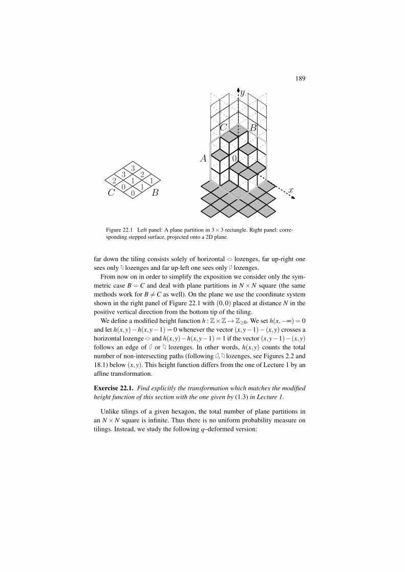
189
0A
x
y
C B00 1
1 12
23
3
C B
Figure 22.1 Left panel: A plane partition in 3× 3 rectangle. Right panel: corre-sponding stepped surface, projected onto a 2D plane.
far down the tiling consists solely of horizontal lozenges, far up-right onesees only lozenges and far up-left one sees only lozenges.
From now on in order to simplify the exposition we consider only the sym-metric case B = C and deal with plane partitions in N×N square (the samemethods work for B 6= C as well). On the plane we use the coordinate systemshown in the right panel of Figure 22.1 with (0,0) placed at distance N in thepositive vertical direction from the bottom tip of the tiling.
We define a modified height function h : Z×Z→ Z≥0. We set h(x,−∞) = 0and let h(x,y)−h(x,y−1) = 0 whenever the vector (x,y−1)− (x,y) crosses ahorizontal lozenge and h(x,y)−h(x,y−1) = 1 if the vector (x,y−1)−(x,y)follows an edge of or lozenges. In other words, h(x,y) counts the totalnumber of non-intersecting paths (following , lozenges, see Figures 2.2 and18.1) below (x,y). This height function differs from the one of Lecture 1 by anaffine transformation.
Exercise 22.1. Find explicitly the transformation which matches the modifiedheight function of this section with the one given by (1.3) in Lecture 1.
Unlike tilings of a given hexagon, the total number of plane partitions inan N×N square is infinite. Thus there is no uniform probability measure ontilings. Instead, we study the following q–deformed version:
190 Lecture 22: Plane partitions and Schur functions.
Definition 22.2. Let Volume(π) be the volume of a plane partition π , whichis the sum of all N2 integers in the table. Given 0 < q < 1, define the qVolume
probability measure on plane partition in N×N square through
PN,q(π) ∝ qVolume(π).
If the parameter q is small, then a typical PN,q–random partition has just afew boxes. On the other hand, as q→ 1, the number of boxes grows to infinityand we can expect non-trivial asymptotic theory.
22.2 Schur Functions
Our treatment of random plane partitions uses Schur polynomials and theircombinatorics. We refer to [Macdonald95, Chapter I] for the detailed treatmentof symmetric polynomials and only review the necessary facts here.
Let GTN denote the set of all N–tuples of integers λ1 ≥ λ2 ≥ ·· · ≥ λN . Inrepresentation-theoretic context, elements of GTN are often called signaturesand the notation GT comes from the names of Gelfand and Tsetlin, who in-troduced an important basis (parameterized by a sequence of signatures) in anirreducible representation of unitary group U(N).
Definition 22.3. Given~k = (k1, . . . ,kN) ∈ ZN , define
a~k(x1, . . . ,xN) = det
xk1
1 · · · xkN1
.... . .
...xk1
N · · · xkNN
= ∑σ∈SN
sign(σ)xkσ(1)1 · · ·x
kσ(N)
N ,
where the sum is taken over all permutations. Given an λ ∈ GTN and settingδ = (N− 1,N− 2, . . . ,0), define the Schur symmetric (Laurent) polynomialsthrough
sλ (x1, . . . ,xN) =aλ+δ (x1, . . . ,xN)
aδ (x1, . . . ,xN).
Exercise 22.4. The denominator aδ is known as Vandermonde determinant.Check that
aδ (x1, . . . ,xN) = ∏1≤i< j≤N
(xi− x j).
Two signatures λ ∈GTN and µ ∈GTN−1 interlace denoted µ ≺ λ if
λ1 ≥ µ1 ≥ λ2 ≥ µ2 ≥ ·· · ≥ µN−1 ≥ λN .
191
Lemma 22.5 (Branching Rule). For any λ ∈GTN , we have
sλ (x1, . . . ,xN) = ∑µ∈GTN−1,µ≺λ
x|λ |−|µ|1 sµ(x2, . . . ,xN), (22.1)
where |λ |= λ1 + · · ·+λN and |µ|= µ1 + · · ·+µN .
Proof If ~= (λ1+N−1, . . . ,λN) and ~m= (µ1+N−2, . . . ,µN−1), then µ ≺ λ
means that
`1 > m1 ≥ `2 > m2 ≥ ·· · ≥ `N .
Multiplying the right hand side of (22.1) by aδ (x1, . . . ,xN) gives
`1−1
∑m1=`2
· · ·`N−1−1
∑mN−1=`N
x|λ |−|µ|1 ∑τ∈SN−1
sign(τ)xm1τ(2) · · ·x
mN−1τ(N)
N
∏i=2
(x1− xi).
Here we consider the action of τ ∈ SN−1 on 2, . . . ,N. Writing
|λ |− |µ|= (`1−m1−1)+ · · ·(`N−1−mN−1−1)+ `N ,
the summation becomes
∑τ∈SN−1
sign(τ)x`N1
`1−1
∑m1=`2
x`1−m1−11 xm1
τ(2)(x1− xτ(2))
· · ·`N−1
∑mN−1=`N
x`N−1−mN−1−11 xmN
τ(N)(x1− xτ(N)).
Each interior summation telescopes, so we obtain
∑τ∈SN−1
sign(τ)x`N1 (x`1−`2
1 x`2τ(2)− x`1
τ(2)) · · ·(x`N−1−`N1 x`N
τ(N)− x`N−1
τ(N)).
The last sum is the determinant of the following N×N matrix:0 x`1−`2
1 (x`12 − x`2
2 ) . . . x`1−`21 (x`1
N − x`2N )
...0 x`N−1−`N
1 (x`N−12 − x`N
2 ) . . . x`N−1−`N1 (x`N−1
N − x`NN )
x`N1 x`N
2 . . . x`NN
We perform elementary manipulations preserving the determinant on the lastmatrix. Adding to the (N− 1)st row the Nth row multiplied by x`N−1−`N
1 webring the (N − 1)st row to the form x`N−1
i . Further adding to (N − 2)nd rowa proper multiple of (N − 1)st row we bring the (N − 2)nd row to the formx`N−2
i . Further repeating this procedure, we bring the matrix to the form (x` ji ),
matching the left-hand side of (22.1).
192 Lecture 22: Plane partitions and Schur functions.
Lemma 22.6 (Cauchy Identity). For |x1|, . . . , |xN |, |y1|, . . . , |yN |< 1, we have
N
∏i, j=1
11− xiy j
= ∑λ∈GTN ,λN≥0
sλ (x1, . . . ,xN)sλ (y1, . . . ,yN).
Proof The Cauchy determinant formula of (20.7) reads
det[
1ui− v j
]N
i, j=1=
∏1≤i< j≤N
(ui−u j)(v j− vi)
N∏
i, j=1(ui− v j)
which implies
det[
11− xiy j
]N
i, j=1=
∏1≤i< j≤N
(xi− x j)(yi− y j)
N∏
i, j=1(1− xiy j)
= aδ (~x)aδ (~y)N
∏i, j=1
(1−xiy j)−1.
On the other hand,
det[
11− xiy j
]N
i, j=1= det
[∞
∑n=0
(xiy j)n
]N
i, j=1
=∞
∑α1=0· · ·
∞
∑αN=0
det[x
α ji y
α jj
]N
i, j=1
=∞
∑α1=0· · ·
∞
∑αN=0
aα(~x)yα11 · · ·y
αNN = ∑
λ∈GTN ,λN≥0aλ+δ (~x)aλ+δ (~y). (22.2)
Dividing by aδ (~x), aδ (~y) completes the proof.
22.3 Expectations of observables
We do not have direct access to the distribution of the value of the height func-tion of random plane partitions at a particular point. However, we can producecontour integral formulas for the expectations of certain polynomial sums inthese values, which we call observables. They are rich enough to fully charac-terize the distribution and therefore are useful for the asymptotic analysis.
The main purpose of this section is to obtain the following formula for theexpectations of observables of the random height function distributed accord-ing to PN,q.
193
Theorem 22.7. Let −N < x1 ≤ ·· · ≤ xk < N and 0 < t1, . . . , tk < 1. Then
E
[k
∏i=1
∑y∈Z
h(xi,y)tyi
]
=1
(2πi)k
˛· · ·
˛∏
1≤i< j≤k
(z j− tit j
zi)(z j− zi)
(z j− tizi)(z j− 1t j
zi)
k
∏i=1
Gxi(zi; ti)dzi
(t−1i −1)(1− ti)zi
,
(22.3)
where
Gx(z; t) = tmin(0,x)∏
i∈Z+ 12
−N<i<min(0,x)
1− t−1q−iz−1
1−q−iz−1 ∏i∈Z+ 1
2max(0,x)<i<N
1−qiz1− tqiz
.
(Note that the sum ∑y∈Z h(xi,y)tyi is infinite only in the positive y direction, as
h(xi,y) vanishes for sufficiently small y,.) The contours satisfy the followingproperties:
• the zi-contour includes the poles at 0,qN− 12 ,qN− 3
2 , . . . ,qmin(0,x)− 12 ,
but does not contain any of the poles att−1i q−max(0,x)− 1
2 ,t−1i q−max(0,x)− 3
2 ,. . . , t−1i q−N+ 1
2 ,• for 1≤ i < j ≤ k we have |tizi|< |z j| everywhere on the contours.
Exercise 22.8. Show that the residue of the integrand in (22.3) at zi = t jz j,1 ≤ i < j ≤ k (but not for i > j) vanishes. In other words, it does not matterwhether the integration contours are nested in such a way that |zi| < |t jz j| or|zi|> |t jz j|, 1≤ i < j ≤ k, — the integral is the same for both choices.
Remark 22.9. A skew plane partition is a generalization in which we placeintegers not in a rectangular table, but in a difference between a rectangle anda Young diagram. Theorem 22.7 has an extension to qVolume–weighted skewplane partitions, see [Ahn18] for the details.
In the rest of the lecture we outline the main ideas for the proof of the theo-rem.
We first observe that a plane partition π in the N×N square grid may beviewed as a sequence of interlacing signatures
( /0)= π−N ≺ π
−N+1≺ ·· · ≺ π−1≺ π
0 π1 ·· · π
N−1 πN =( /0). (22.4)
In the notations of the left panel of Figure 22.1, each signature represents avertical slice of the picture, so that π−N+1 ∈ GT1, . . . ,π
0 ∈ GT0, . . . ,πN−1 ∈
194 Lecture 22: Plane partitions and Schur functions.
GTN . The slice are read from left to the right. In particular, the plane partitionof Figure 22.1 corresponds to the sequence
( /0)≺ (2)≺ (3,0)≺ (3,1,0) (2,1) (1) ( /0).
In what follows, we often treat a signature λ ∈GTN (with non-negative coor-dinates) as a signature µ ∈GTM with M > N by adding sufficiently many zerolast coordinates. For instance, (2,1)∈GT2 can be treated as (2,1,0)∈GT3 oras (2,1,0,0) ∈GT4.
Lemma 22.10. Fix x ∈ −N +1,−N +2, . . . ,N−1 and take arbitrary M ≥N−|x|. Let λ ∈GTM be the signature encoding the vertical slice of the planepartition at abscissa x, i.e. λ is πx with M−N + |x| additional zeros. For any0 < t < 1, we have
∑y∈Z
h(x,y)ty =tmin(0,x)
1− t
(M
∑i=1
tλi−i+1− t−M+1
1− t
).
Proof The appearance of min(0,x) in the formulas is related to our particularchoice of the coordinate system, as in the right panel of Figure 22.1. The ithfrom top horizontal lozenge in the vertical section of the tilings at abscissa xhas top and bottom coordinates πx
i − i+ 1+min(0,x) and πxi − i+min(0,x),
respectively. With this in mind and using that h(x,y)−h(x,y−1) = 1 unless ycorresponds to the top of a horizontal lozenge, we compute
∑y∈Z
h(x,y)ty =1
1− t ∑y∈Z
h(x,y)(ty− ty+1)
=1
1− t ∑y∈Z
(h(x,y)−h(x,y−1))ty
=1
1− t ∑y∈Z
(1−1[y ∈ πxi − i+1+min(0,x)∞
i=1])ty
=1
1− t ∑y>−M+min(0,x)
(1−1[y ∈ πxi − i+1+min(0,x)M
i=1])ty
=1
1− t
(−
M
∑i=1
tπxi −i+1+min(0,x)+
t−M+1+min(0,x)
1− t
),
where in the third line πx is extended to have infinitely many coordinates byadding (infinitely many) zeros, in the forth line πx is extended to an elementof GTM (by adding M−N + |x| zeros), and the last line is obtained from theforth by summing 1’s and indicators 1 separately.
195
In view of the previous lemma, set
℘t(λ ) =M
∑i=1
tλi−i+1− t−M+1
1− t, λ ∈GTM, λM ≥ 0.
Note that if we increase M and simultaneously extend λ by adding zeros, then℘t(λ ) is unchanged.
Our plan is to compute expectations of products of ℘t(πx), and then use the
previous lemma to obtain Theorem 22.7. This is achieved using the followingfamily of difference operators.
Definition 22.11. The first Macdonald operator Dx1,...,xnt is defined by
Dx1,...,xnt =
n
∑i=1
[∏j 6=i
xi− t−1x j
xi− x j
]Tt,xi −
t−n+1
1− t
where Tt,xi is the t–shift operator which maps
F(x1, . . . ,xi−1,xi,xi+1, . . . ,xN) 7→ F(x1, . . . ,xi−1, txi,xi+1, . . . ,xN).
Remark 22.12. The operators Dx1,...,xnt are q= t versions of the difference op-
erators used by Ian Macdonald in his study of the (q, t)–deformation of Schurpolynomials bearing his name, see [Macdonald95, Chapter VI].
Lemma 22.13. The operator Dx1,...,xnt is diagonalized by the Schur functions
sλ (x1, . . . ,xn), λ ∈GTN . We have
Dx1,...,xnt sλ (x1, . . . ,xn) =℘t(λ )sλ (x1, . . . ,xn).
Proof Observe that(D~x
t +t−n+1
1− t
)sλ (~x)= t−n+1
n
∑i=1
[∏j 6=i
txi− x j
xi− x j
]Tt,xiaλ+δ (~x)
Tt,xiaδ (~x)=
n
∑i=1
Tt,xiaλ+δ (~x)aδ (~x)
where the second equality uses that the txi−x jxi−x j
terms replace the t-shifted fac-tors in Tt,xiaδ (~x) with the corresponding ordinary factors in aδ (~x). Writing thealternant as
aλ+δ (~x) = ∑σ∈Sn
sgn(σ)n
∏j=1
xλσ( j)+n−σ( j)j
we have thatn
∑i=1
Tt,xiaλ+δ (~x) =
(n
∑i=1
tλi+n−i
)aλ+δ (~x)
which implies the statement of the lemma.
196 Lecture 22: Plane partitions and Schur functions.
We are able produce a contour integral representation for the action of theseoperators on multiplicative functions ∏
ni=1 f (xi):
Lemma 22.14 ([BorodinCorwin11]). Let f (z) be analytic and q∈C such thatf (qz)f (z) has no singularities in this neighborhood of xin
i=1. Then
D~xt
n
∏i=1
f (xi) =n
∏i=1
f (xi)
˛ n
∏j=1
z− t−1x j
z− x j· f (tz)
f (z)dz
(1− t−1)z,
where the contour contains 0 and xini=1 and no other singularities of the
integrand.
Proof This follows from the residue theorem and the definition of the opera-tor D~x
t .
The idea of the proof of Theorem 22.7 is to use the Dt operators to extractthe volume information relying on the following lemma:
Lemma 22.15. Let F denote a function of 2N variables a1, . . . ,aN , b1, . . .bN
given by
F =N
∏i, j=1
11−aib j
. (22.5)
Then for qVolume random plane partitions identified with interlacingsequences of signatures through (22.4), any −N < x1 ≤ ·· · ≤ xk ≤ 0,N > x′1 ≥ ·· · ≥ x′k′ ≥ 0, and any 0 < ti, t ′i < 1, we have
E[℘t1(π
x1) · · ·℘tk(πxk) ·℘t1(π
x′1) · · ·℘t ′k(πx′k′ )
]=
[F−1D
aN ,...,aN+x1t1 · · ·D
aN ,...,aN+xktk D
bN ,...,bx′1−1
t ′1· · ·
· · ·DbN ,...,bx′k−1
t ′kF]
ai=bi=qi−1/2, i=1,...,N. (22.6)
Exercise 22.16. Given Lemma 22.15, prove Theorem 22.7 by a recursive ap-plication of Lemma 22.14 to convert the right-hand side (22.6) into contourintegrals.
Let us present a historic overview for Lemma 22.15. Connection be-tween plane partitions and Schur polynomials was first exploited in prob-abilistic context in [OkounkovReshetikhin01]. The use of the differentialoperators for the case k′ = 0 and x1 = x2 = · · · = xk was introduced in[BorodinCorwin11]. The extension to arbitrary xi (still k′ = 0) was pre-sented in [BorodinCorwinGorinShakirov13, Section 4]. An observation that
197
k′ > 0 is also possible can be found in [BufetovGorin17, Section 3]. Also[BorodinCorwinGorinShakirov13, Section 3] presents another way to reachTheorem 22.14 avoiding k′ > 0 case, and [Aggarwal14, Proposition 2.2.4] isa generalization of Theorem 22.14 obtained by this method. We also refer to[Ahn18] where another set of difference operators is used to extract observ-ables of plane partitions.
We only present the k = 1, k′ = 0 case of Lemma 22.15; general case is anextension of the arguments below and details can be found in the aforemen-tioned references.
Proof of k = 1, k′ = 0 case of Lemma 22.15 The first observation is that withthe notation |π i|= π i
1 +π i2 + . . . , we have
qVolume(π) = q12 (|π0|−|π1|)q
32 (|π1|−|π2|) · · ·q(N−
12 )|πN−1|
×q12 (|π0|−|π−1|)q
32 (|π−1|−|π−2|) · · ·q(N−
12 )|π−N+1|.
Hence, if we take an expression
∑λ∈GTN λN≥0
sλ
(qN− 1
2 ,qN− 32 , . . . ,q1/2
)sλ
(qN− 1
2 ,qN− 32 , . . . ,q1/2
)and expand both sλ factors into sums of monomials by recursively using thebranching rule of Lemma 22.5, then each term in the expanded sum corre-sponds to a plane partition as in (22.4) and the value of such term is preciselyqVolume(π).
We can also first expand
∑λ∈GTN ,λN≥0
sλ (a1, . . . ,aN)sλ (b1, . . . ,bN) (22.7)
into monomials in ai, bi, getting a sum over plane partitions and substituteai = bi = qi−1/2 later on. Note that (22.7) evaluates to the function F of (22.5)by Lemma 22.6. In particular, we get
[F ]ai=bi=qi−1/1 = ∑π
qVolume(π). (22.8)
Assume without loss of generality that x1 ≤ 0. Let us expand (22.7) intomonomials corresponding to plane partitions π , then fix πx1 ,πx1+1, . . . ,πN−1
and make a summation over π1−N ,π2−N , . . . ,πx1−1. We claim that the resulthas the form
sπx1 (aN ,aN−1, . . . ,a1−x1)× (terms depending on a−x1 , . . . ,a1, b1, . . . ,bN).
(22.9)Indeed, the summation goes over interlacing signatures, hence, we can again
198 Lecture 22: Plane partitions and Schur functions.
use Lemma 22.5 to turn the result into the Schur function. We can now actwith D
aN ,aN−1,...,a1−x1t on F , by using (22.9) and eigenrelation of Lemma
22.13. The factor ℘t(πx1) pops out, and afterwards we can again expand
sπx1 (aN ,aN−1, . . . ,a1−x1) into monomials. The conclusion is that[
DaN ,aN−1,...,a1−x1t F
]ai=bi=qi−1/2
= ∑π
℘t(πx1)qVolume(π).
Dividing by F and using (22.8) we get the desired evaluation of E℘t(πx1).
Exercise 22.17. Using (22.8) compute the partition function of qVolume–weighted plane partitions, i.e. show that1
∑plane partitions
qVolume =∞
∏n=1
(1−qn)−n, (22.10)
where the sum is taken over all plane partitions, which is the N = ∞ version ofthe ones in Definition 22.2.
1 Similarly to (1.1), this formula also bears the name of Macmahon and has been known formore than 100 years, although the first proofs were not using Schur polynomials.
Lecture 23: Limit shape and fluctuationsfor plane partitions.
In this lecture we use Theorem 22.7 to analyze global asymptotics (LLN andCLT) for random qVolume–weighted plane partitions.
In what follows we fix N > 0 and set q = e−ε , N = bN/εc for a small pa-rameter ε > 0.
Our goal is to show that for the random height function h(x,y) of planepartitions in N ×N rectangle and distributed according toPN,q of Definition22.2, we have as ε → 0
εh(
xε,
yε
)→ h∞(x, y)
h(
xε,
yε
)−Eh
(xε,
yε
)→ GFF
where h∞ is a deterministic limit shape, and GFF is the Gaussian Free Fieldgoverning fluctuations.
23.1 Law of Large Numbers
Our first result is the limit shape theorem for the height function of the qVolume–weighted random plane partitions in N×N rectangle.
Theorem 23.1. For any x ∈ [−N, N] and c > 0, we have
limε→0
E
[∑
y∈εZε
2h(
xε,
yε
)e−cy
]→
ˆh∞(x, y)e−cy dy, (23.1)
where h∞ is an explicit function described in Theorem 23.5 below.
199
200 Lecture 23: Limit shape and fluctuations for plane partitions.
Remark 23.2. In the next section we show that the variance of the height func-tion decays, which automatically upgrades the convergence of expectations in(23.1) to convergence in probability.
Remark 23.3. Formally, the height function h(x,y) is defined only at integerpoints (x,y), and therefore, we should write h
(⌊ xε
⌋, y
ε
), where b·c is the inte-
ger part. However, we are going to omit the integer part in order to simplifythe notations.
The proof of Theorem 23.1 starts by expressing (23.1) as a contour integral.
Lemma 23.4. For any c > 0 we have
limε→0
E
[∑
y∈εZε
2h(
xε,
yε
)e−cy
)=
12πi
˛0Gx(z)c dz
c2z, (23.2)
where
Gx(z) =1− z
e−N− z· e−x− z−1
e−N− z−1, (23.3)
the branch for raising to the cth power is the one giving positive real valuesto z = 0 and z = ∞, and integration goes over a positively oriented contourenclosing 0 and [e−N ,e−min(0,x], but not [emax(0,x),eN ].
Proof The k = 1 case of Theorem 22.7 reads
E
[∑y∈Z
h(x,y)ty
]=
12πi
˛Gx(z; i)
dz(t−1−1)(1− t)z
, (23.4)
where
Gx(z; t) = tmin(0,x)∏
i∈Z+ 12
−N<i<min(0,x)
1− t−1q−iz−1
1−q−iz−1 ∏i∈Z+ 1
2max(0,x)<i<N
1−qiz1− tqiz
,
and the integration contour includes the poles at 0,qN− 12 ,qN− 3
2 , . . . ,qmin(0,x)− 12 .
We set
t = exp(−cε), q = exp(−ε), x =xε, y =
yε, N =
Nε
and send ε → 0. Let us analyze the asymptotic behavior of Gx(z; t). Clearly,tmin(0,x) → e−cmin(0,x). Using the asymptotic expansion ln(1+ u) = u+ o(u),
201
the logarithm of the first product in Gx(z, t) behaves as:
∑i∈Z+ 1
2−N/ε<i<min(0,x/ε)
ln(
1− t−1q−iz−1
1−q−iz−1
)
= ∑i∈Z+ 1
2−N/ε<i<min(0,x/ε)
(1− t−1)q−iz−1
1−q−iz−1 +o(1)
=1− t−1
1−q ∑i∈Z+ 1
2−N/ε<i<min(0,x/ε)
(q−i−q−i+1)z−1
1−q−iz−1 +o(1)
=−cˆ emin(0,x)
e−N
z−1
1−uz−1 du+o(1) = cˆ emin(0,x)
e−N
1u− z
du+o(1)
= c ln
(emin(0,x)− z
e−N− z
)+o(1).
Note that the logarithm of complex argument is a mutlivalued function andhere we mean the branch which gives 0 for z = ∞ in the last formula (and areal number at z = 0). The convergence is uniform over z in compact subsetsof C\ [exp(−N),exp(min(0, x))].
Similarly, the asymptotic behavior of the logarithm of the second product inGx(z, t) is
c ln
(e−max(0,x)− z−1
e−N− z−1
)
with uniform convergence on compact subsets of C \ [emax(0,x),eN ] and thebranch of logarithm, which gives 0 at z = 0 in the last formula (and a realnumber at z = ∞). Combining the factors, we get
limε→0
Gx/ε(z; t) =
(e−min(0,x) emin(0,x)− z
e−N− z· e−max(0,x)− z−1
e−N− z−1
)c
, (23.5)
where the convergence is uniform over compact subsets ofC \ [exp(−N),exp(min(0, x))] \ [emax(0,x),eN ] and the branch for the c-thpower is the one giving positive real values for z = 0 and z = ∞. Checkingseparately cases x≤ 0 and x≥ 0, one sees that (23.5) is the same expression as(
1− z
e−N− z· e−x− z−1
e−N− z−1
)c
.
202 Lecture 23: Limit shape and fluctuations for plane partitions.
Passing to the limit ε → 0 in the integrand of the contour integral (23.4), weget the result.
The next step is to show that the right-hand side of (23.2) as a function of cis the Laplace transform of a function; that is, there exists h∞(x, y) such that
ˆ∞
−∞
h∞(x, y)e−cy dy =1
2πi
˛Gx(z)c dz
c2z.
This function h∞(x, y) can be described quite exactly. Let us outline the com-putation of its derivative, for a more detailed argument see [Ahn18, Proof ofCorollary 6.3]. We begin by integrating by parts:
ˆ∞
−∞
∂yh∞(x, y)e−cy dy = cˆ
∞
−∞
h∞(x, y)e−cy dy =1
2πi
˛Gx(z)c dz
cz. (23.6)
Define
µx(u) := ∂yh∞(x, y)|e−y=u.
The left-hand side of (23.6) can be rewritten asˆ
∞
−∞
∂yh∞(x,y)e−cy dy =ˆ
∞
0µx(u)uc du
u.
Information on the moments of the measure µx(u)du allows us to write downits Stieltjes transform:
Sµx(w) :=ˆ
∞
0
µx(u)duw−u
=∞
∑c=1
1w−c
ˆ∞
0µx(u)uc du
u
=∞
∑c=1
w−c 12πi
˛Gx(z)c dz
cz=
12πi
˛ln(
1− Gx(z)w
)dzz. (23.7)
Here, the forth equality is obtained by interchanging the sum and integral,and recognizing the internal expression as the power series expansion of thelogarithm. The parameter w should be chosen to be very large to guarantee theconvergence of the sums, and the contour in the integral is as in Lemma 23.4,i.e. it encloses 0 and e−N , but not eN .
The integrand has two singularities inside the integration contour: simplepole at z = 0 and a more complicated singularity at the root of the equationGx(z) = w close to e−N (since Gx(z) has a simple pole at e−N , such root existsand is unique for large w). Let us denote this root through z0 and let γ be a
203
contour enclosing z0. Integrating by parts, we have
Sµx(w) = ln(
1− Gx(0)w
)+
12πi
˛γ
ln(
1− Gx(z)w
)dzz
= ln(
1− Gx(0)w
)+
12πi
˛γ
G ′x(z)Gx(z)−w
ln(z)dz. (23.8)
The last integral has a simple pole at z0 with residue ln(z0). Using also theexplicit value for Gx(0), we conclude that
Sµx(w) = ln
(1− eN
w
)+ ln(z0), (23.9)
where z0 is still the root of the equation
w = Gx(z) (23.10)
in a neighborhood of e−N .By its definition, the Stieltjes transform Sµx(w) is a complex analytic func-
tion of w outside of the (real) support of µx. Hence, we can analytically con-tinue the formula (23.9) from large w to arbitrary w; the formula will remainthe same, with the only difference being in the choice of the root of (23.10) —we no longer can guarantee that the desired root is the one closest to e−N .
After we figure out the Stieltjes transform, we can reconstruct the measuresµx(u)du itself. For that note that when w crosses the real axis at a real pointu, the imaginary part of Sx makes a jump1 by 2πµx(u). We conclude that2π∂yh∞(x, y) is the jump of the imaginary part of (23.9) at the point w = e−y.Note that we expect the limit shape h∞(x, y) to be identical 0 for y ≤ −N be-cause of our choice of definition of the height function (alternatively, this canalso be shown by analyzing the function Sµx(w)). Thus, we can further consider
only y > −N. Then for the first term in (23.9) we notice that eN
w = eN+y > 1.Hence, imaginary part of the logarithm makes a jump by 2π .
For the second term in (23.9), note that upon substitution w = e−y and def-inition of Gx(z) from (23.3), we transform (23.10) into a quadratic equationin z with real coefficients. It either has real roots (in which case, there is nointeresting jump for ln(z0)), or complex conjugate roots. One can check thatthe jump of ln(z0) comes precisely from the choice of the root in the upperhalf-plane changing to the choice of the one in the lower half-plane. Hence,the jump of the imaginary part of ln(z0) is twice the argument of z0. Let usrecord our findings in the theorem.
1 For simplicity, assume that u is a point of continuity of µx. Then this fact is proven by directcomputation of the imaginary part as we approach u from the upper and lower halfplanes.
204 Lecture 23: Limit shape and fluctuations for plane partitions.
Theorem 23.5. Let ζ (x, y) be a root of the quadratic equation
1− z
e−N− z· e−x− z−1
e−N− z−1= e−y (23.11)
chosen so that ζ (x, y) is continuous in (x, y) and ζ is in the upper half-planeH, if (23.11) has two complex conjugate roots. Then
∂yh∞(x, y) = 1− argζ (x, y)π
.
Remark 23.6. Notice that if ζ (x, y) is real, then ∂yh∞(x, y) = 0 or 1. This corre-sponds to the frozen region, either beneath the partition (where h is not chang-ing) or above the partition (where the image is vertical, and h increases withy). For (x, y) such that z(x, y) ∈H, we have
0 < ∂yh∞(x, y)< 1.
This corresponds exactly to the liquid region D. Therefore, the liquid regionmay be alternatively defined as the set of (x, y) ∈ R2 such that (23.11) has apair of complex conjugate roots.
Remark 23.7. Let us match the result of Theorem 23.5 with Kenyon-Okounkovtheory developed in Lectures 9 and 10. We define a complex number z, so that
ζ (x, y) = ex(1− z(x, y)).
Note that since ζ is in the upper half-plane, so is z. Conjugating the equation(23.11) and rewriting it in terms of z, we get
Q(zey,(1− z)ex) = 0, Q(u,v) = u(1− v)− (e−N− v)(1− ve−N).
This is precisely the equation of the form appearing in Theorems 9.8, 10.1 andgiving solutions to the complex Burgers equation for the limit shape. Indeed,the parameter c appearing in those theorems is−1 in our setting, see Corollary9.6 and identify ε with 1/L. Note also that arg(ζ ) is computing the densityof horizontal . Hence, this density is also computed by −arg(1− z), whichmatches Figure 9.1. With a bit more care, one can show that z(x, y) is preciselyKenyon–Okounkov’s complex slope.
Exercise 23.8. Extend Theorems 23.1 and 23.5 to qVolume–weighted plane par-titions in N×bαNc rectangle, α > 0, as N→ ∞.
Exercise 23.9. Sending N→ ∞ in the result of Theorem 23.5 we get the limitshape for the plane partitions without bounding rectangle. Find explicitly theformula for the boundary of the frozen region in this situation. The answer(drawn on the plane of the right panel of Figure 22.1) should be invariantunder rotations by 120 degrees.
205
The limit shape theorem for the qVolume–weighted plane partitions (with-out bounding rectangle) was first announced in [Vershik97]. The mathematicalderivations soon appeared in [CerfKenyon01] and [OkounkovReshetikhin01].
23.2 Central Limit Theorem
Our next aim is to show that the centered height function
√π
[h(
xε,
yε
)−Eh
(xε,
yε
)]converges to the pullback of the Gaussian free field (GFF) under the mapζ (x, y) from Theorem 23.5.
We briefly recall the definition of the GFF, see Lecture 11 for more details.
Definition 23.10. The Gaussian Free Field on the upper half-plane H= z ∈C | ℑ(z)> 0 is a random generalized centered Gaussian function GFF on Hwith covariance
EGFF(z)GFF(w) =− 12π
log∣∣∣∣ z−wz− w
∣∣∣∣ .Given a bijection ζ : D→H, where D⊂ R2, we define the GFF pullback.
Definition 23.11. The ζ -pullback of the GFF is a random distribution GFF ζ
such that
E[GFF ζ (x1,y1)GFF ζ (x2,y2)] =−1
2πlog∣∣∣∣ζ (x1,y1)−ζ (x2,y2)
ζ (x1,y1)− ζ (x2,y2)
∣∣∣∣ .Theorem 23.12. For the height functions of qVolume–weighted plane partitions,we have√
π ∑y∈εZ
ε
(h(
xε,
yε
)−Eh
(xε,
yε
))e−cy
c>0,−N≤x≤N
→ˆ
Dx
H ζ (x, y)e−cy
c>0,−N≤x≤N(23.12)
in the sense of convergence of finite dimensional distributions as ε → 0. Hereζ (x, y) is as in Theorem 23.5, D is the liquid region (which can be defined asthose (x, y), for which ζ is non-real), and Dx is the section of D by the verticalline with abscissa x.
206 Lecture 23: Limit shape and fluctuations for plane partitions.
Remark 23.13. By Remark 23.7, ζ = ex(1− z), where z is the Kenyon–Okounkov’s complex slope. Since also Q(eyz,ex(1− z)) = 0 for analytic Q,the complex structure of ζ is the same as the one of eyz. Noting also that theLaplacian in the definition of the GFF is unchanged under the conjugation ofthe complex structure, we conclude that Theorem 23.12 is precisely a particu-lar case of Conjecture 11.1.
Exercise 23.14. Show that ζ : D→H is a homeomorphism from D to H, whichmaps sets of the form (x,y) ∈ D : y ∈ R for fixed x to half circles in H withreal center points.
The convergence in the sense of finite dimensional distributions in Theorem23.12 means that if we take any finite collection
c1, . . . ,ck, −N ≤ x1, . . . , xk ≤ N,
then we have the convergence in distribution for random vectors
limε→0
(∑
y∈εZε
(h(
xi
ε,
yε
)−Eh
(xi
ε,
yε
))e−ci y
)k
i=1
=
(ˆDxi
H ζ (x, y)e−ci ydy
)k
i=1
. (23.13)
We can prove such a statement by showing that the random vectors aboveconverge to a Gaussian limit and then matching their covariance. We outlinesome of the ideas of the proof here and refer to [Ahn18] for more details.
Definition 23.15. Given random variables X1, . . . ,Xn, their joint mixed cumu-lant κ(X1, . . . ,Xn) is defined as
κ(X1, . . . ,Xn) =∂ n
∂ t1 . . .∂ tnlnE
[exp
(i
N
∑i=1
tiXi
)]∣∣∣∣∣t1=t2=···=tn=0
.
If we fix random variables Y1, . . . ,Yk, then its family of cumulants are definedas all possible κ(X1, . . . ,Xn), n = 1,2, . . . , where Xi coincide with various Yj
with possible repetitions. n is then the order of the cumulant. For instance, ifwe have one random variable Y1 = Y , then its first cumulant is κ(Y ) = EY ,and the second cumulant κ(Y,Y ) = EY 2− (EY )2. For two random variablesthe second order cumulant is the covariance, κ(X1,X2) = cov(X1,X2).
For a Gaussian vector (Y1, . . . ,Yk), the logarithm of its characteristic functionis a second degree polynomial. This leads to the following statement:
207
Exercise 23.16. A random vector (Y1, . . . ,Yk) has Gaussian distribution if andonly if all joint cumulants of its coordinates of order ≥ 3 vanish.
In principle, one can express joint cumulants through joint moments. In thisway, vanishing of the higher-order cumulants is equivalent to the Wick’s for-mula for the computation of joint moments for Gaussian vector as a combina-torial sum involving perfect matchings.
Hence, in order to prove Theorem 23.12 we need two steps:
1 Compute the covariance for random variables ∑y∈εZ ε
(h(
xiε, y
ε
))e−ci y us-
ing Theorem 22.7 and show that it converges to the covariance of the vectorsin the right-hand side of (23.13).
2 Compute higher order cumulants for the same random variables and showthat they converge to 0.
We only outline the first step. The asymptotic vanishing of the higher or-der cumulants for the second step holds in much greater generality for randomvariables, whose joint moments are given by contour integrals as in Theorem22.7. We refer to [BorodinGorin13, Section 4.3], [GorinZhang16, Section 6.2],[Ahn18, Section 5.3] for such arguments. For the identification of the covari-ance structure, take c1,c2 > 0 and −N ≤ x1, x2 ≤ N. Then
Cov
(∑
ˆy∈Zε
(h(
x1
ε,
yε
)−Eh
(x1
ε,
yε
))e−c1 y,
∑ˆy∈Z
ε
(h(
x2
ε,
yε
)−Eh
(x2
ε,
yε
))e−c2 y
)
= E
[2
∏i=1
∑y∈Z
εh(
xi
ε,
yε
)e−ci y
]−
2
∏i=1
E
[ε ∑
y∈Zh(
xi
ε,
yε
)e−ci y
].
By Theorem 22.7, the above is
1(2πi)2
˛ ˛ ( (z2− t1t2
z1)(z2− z1)
(z2− t1z1)(z2− 1t2
z1)−1
)2
∏i=1
[Gxi(zi; ti)
εdzi
(t−1i −1)(1− ti)zi
],
where ti = e−ciε , xi =xiε
. Since
(z2− t1t2
z1)(z2− z1)
(z2− t1z1)(z2− 1t2
z1)−1 =
(1− t1)( 1t2−1)z1z2
(z2− t1z1)(z2− 1t2
z1),
the ε factors balance out with 1− ti to give us an overall 1/(c1c2) factor. By
208 Lecture 23: Limit shape and fluctuations for plane partitions.
(23.5), we obtain
1c1c2· 1(2πi)2
˛ ˛Gx1(z1)
c1Gx2(z2)c2
(z2− z1)2 dz1 dz2. (23.14)
It remains to show that (23.14) is the covariance of the GFF paired with expo-nential test functions on the sections.
Let Ci be a closed contour symmetric with respect to the x-axis, and thepart of Ci in H is the half circle which is ζ –image of the vertical section ofthe liquid region with abscissa xi, i.e., the set ζ (xi, y) | y ∈ Dxi. We deformthe integration contours in (23.5) to Ci and then split Ci = C+
i ∪C−i , whereC+
i = Ci ∩H. Changing variables via ζ (x,y) 7→ (x,y) and using (23.11), werewrite (23.14) as
− 14π2c1c2
ˆDx2
ˆDx1
e−c1 y1e−c2 y2
(ζ (x1, y1)−ζ (x2, y2))2∂ζ
∂ y1(x1, y1)
∂ζ
∂ y2(x2, y2)dy1 dy2
+1
4π2c1c2
ˆDx2
ˆDx1
e−c1 y1e−c2 y2
(ζ (x1, y1)−ζ (x2, y2))2
∂ζ
∂ y1(x1, y1)
∂ζ
∂ y2(x2, y2)dy1 dy2
+1
4π2c1c2
ˆDx2
ˆDx1
e−c1 y1e−c2 y2
(ζ (x1, y1)−ζ (x2, y2))2
∂ζ
∂ y1(x1, y1)
∂ζ
∂ y2(x2, y2)dy1 dy2
− 14π2c1c2
ˆDx2
ˆDx1
e−c1 y1e−c2 y2
(ζ (x1, y1)−ζ (x2, y2))2
∂ζ
∂ y1(x1, y1)
∂ζ
∂ y2(x2, y2)dy1 dy2.
(23.15)
Integrate by parts on y1 and y2 for each summand, observing that the boundaryterms cancel since the value of ζ (x, ·) at the end points of Dx is real, to obtain
−14π2
ˆ
Dx2
ˆ
Dx1
e−c1 y1−c2 y1
[log(ζ (x1,y1)−ζ (x2,y1)
)−log
(ζ (x1,y1)−ζ (x2,y1)
)− log
(ζ (x1,y1)−ζ (x2,y1)
)+ log
(ζ (x1,y1)−ζ (x2,y1)
)]dy1 dy1
=− 12π2
ˆDx2
ˆDx1
e−c1 y1e−c2 y1 log
∣∣∣∣∣ζ (x1, y1)−ζ (x2, y1)
ζ (x1, y1)−ζ (x2, y1)
∣∣∣∣∣ dy1 dy2.
This is precisely the desired formula for the covariance of the integrals of theGFF against exponential test functions. The prefactor 1
2π2 matches the one inConjecture 11.1; it also mathes the ratio of 1
2πin Definition 23.11 and (
√π)2
coming from the prefactor in (23.12).
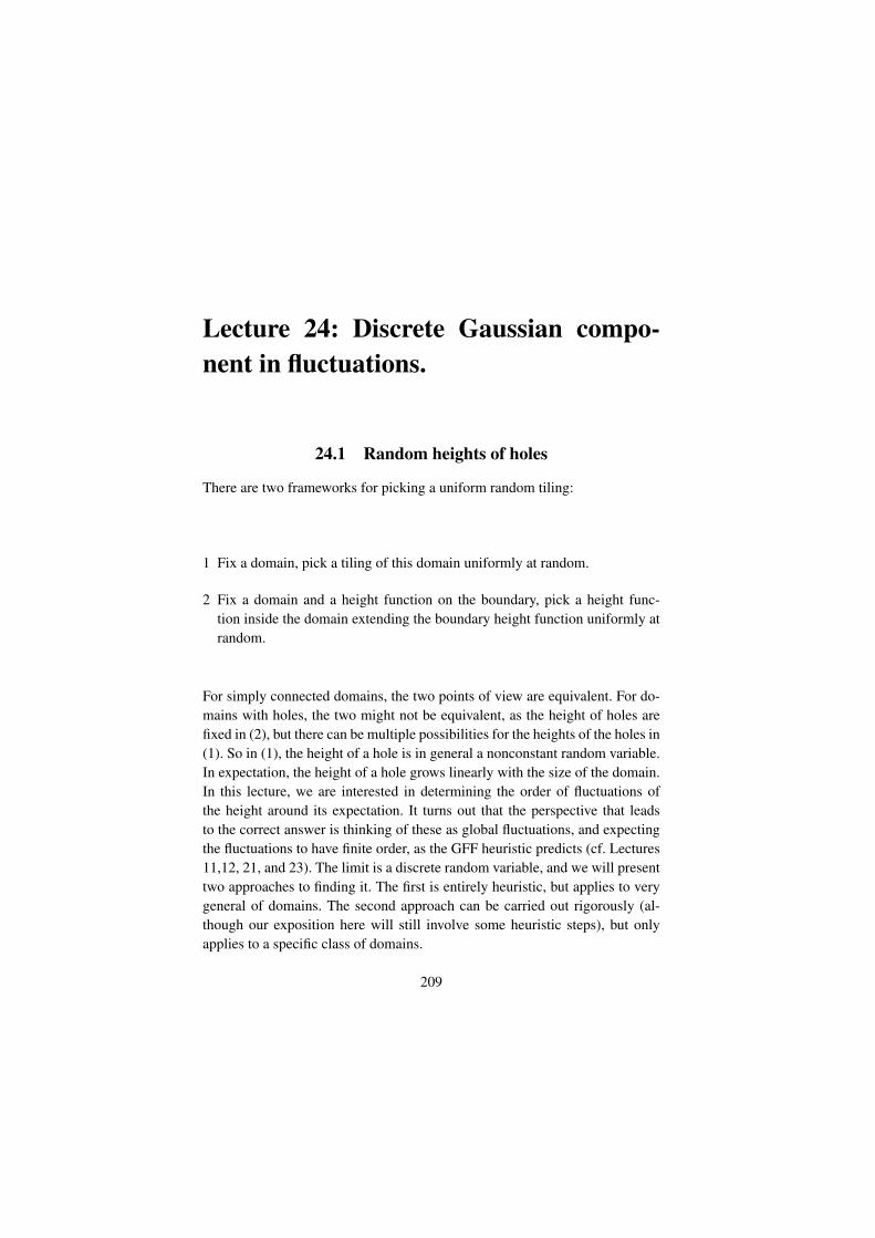
Lecture 24: Discrete Gaussian compo-nent in fluctuations.
24.1 Random heights of holes
There are two frameworks for picking a uniform random tiling:
1 Fix a domain, pick a tiling of this domain uniformly at random.
2 Fix a domain and a height function on the boundary, pick a height func-tion inside the domain extending the boundary height function uniformly atrandom.
For simply connected domains, the two points of view are equivalent. For do-mains with holes, the two might not be equivalent, as the height of holes arefixed in (2), but there can be multiple possibilities for the heights of the holes in(1). So in (1), the height of a hole is in general a nonconstant random variable.In expectation, the height of a hole grows linearly with the size of the domain.In this lecture, we are interested in determining the order of fluctuations ofthe height around its expectation. It turns out that the perspective that leadsto the correct answer is thinking of these as global fluctuations, and expectingthe fluctuations to have finite order, as the GFF heuristic predicts (cf. Lectures11,12, 21, and 23). The limit is a discrete random variable, and we will presenttwo approaches to finding it. The first is entirely heuristic, but applies to verygeneral of domains. The second approach can be carried out rigorously (al-though our exposition here will still involve some heuristic steps), but onlyapplies to a specific class of domains.
209
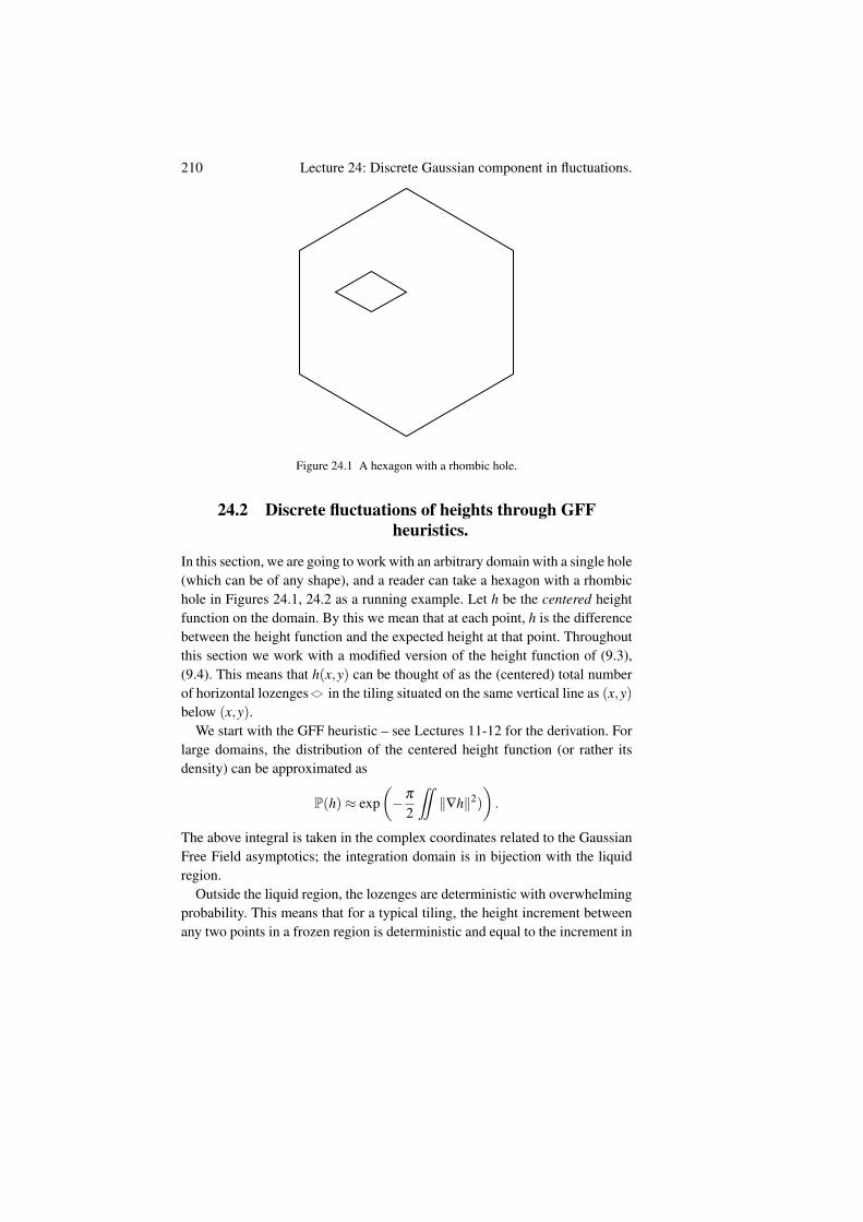
210 Lecture 24: Discrete Gaussian component in fluctuations.
Figure 24.1 A hexagon with a rhombic hole.
24.2 Discrete fluctuations of heights through GFFheuristics.
In this section, we are going to work with an arbitrary domain with a single hole(which can be of any shape), and a reader can take a hexagon with a rhombichole in Figures 24.1, 24.2 as a running example. Let h be the centered heightfunction on the domain. By this we mean that at each point, h is the differencebetween the height function and the expected height at that point. Throughoutthis section we work with a modified version of the height function of (9.3),(9.4). This means that h(x,y) can be thought of as the (centered) total numberof horizontal lozenges in the tiling situated on the same vertical line as (x,y)below (x,y).
We start with the GFF heuristic – see Lectures 11-12 for the derivation. Forlarge domains, the distribution of the centered height function (or rather itsdensity) can be approximated as
P(h)≈ exp(−π
2
¨‖∇h‖2)
).
The above integral is taken in the complex coordinates related to the GaussianFree Field asymptotics; the integration domain is in bijection with the liquidregion.
Outside the liquid region, the lozenges are deterministic with overwhelmingprobability. This means that for a typical tiling, the height increment betweenany two points in a frozen region is deterministic and equal to the increment in
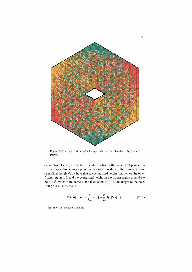
211
Figure 24.2 A typical tiling of a hexagon with a hole. Simulation by LeonidPetrov.
expectation. Hence, the centered height function is the same at all points of afrozen region. So picking a point on the outer boundary of the domain to havecentralized height 0, we have that the centralized height function on the outerfrozen region is 0, and the centralized height on the frozen region around thehole is δ , which is the same as the fluctuation h(B)1 of the height of the hole.Using our GFF heuristic,
P(h(B) = δ )≈ˆ
Ωδ
exp(−π
2
¨‖∇h‖2
), (24.1)
1 h(B) stays for “Height of Boundary”.
212 Lecture 24: Discrete Gaussian component in fluctuations.
where Ωδ is the subset of height functions for which the height of the innerfrozen region is δ .
We would like to understand how (24.1) changes as we vary δ . For that wetake a (unique) harmonic function gδ on the liquid region that satisfies gδ = 0boundary condition on the outer boundary and gδ = δ boundary condition onthe internal boundary surrounding the hole. The harmonicity is with respect tothe local coordinates of the GFF complex structure. Then for h ∈ Ωδ we candefine h = h−gδ , and notice that h is 0 on all boundaries of the liquid region.This takes us a step closer to evaluating the integral:
h = h+gδ
¨‖∇h‖2 =
¨‖∇h+∇gδ‖2 =
¨‖∇h‖2 +
¨‖∇gδ‖2 +2
¨〈∇h,∇gδ 〉
We can integrate the last summand by parts:¨〈∇h,∇gδ 〉= boundary term−
¨h∇
2gδ .
The boundary term is 0 since h is 0 on the boundary, and the other term is 0since ∇2gδ = 0 as gδ is harmonic.
Hence, we can write the probability we are interested in as
P(h(B) = δ )≈ˆ
Ωδ
exp(−π
2
¨‖∇h‖2 +
¨‖∇gδ‖2
).
Notice that for any δ , δg1 is harmonic and satisfies the same boundary condi-tions as gδ , so gδ = δg1. Hence, we can write
P(h(B) = δ )≈ˆ
Ωδ
exp(−π
2
¨‖∇h‖2
)· exp
(−π
2δ
2¨‖∇g1‖2
)= exp(−Cδ
2)
ˆΩδ
exp(−π
2
¨‖∇h‖2
).
Note that h in the last integral is an element of Ω0 and therefore is independentof δ . Hence, the integral evaluates to a δ–independent constant. Therefore, wehave provided a heuristic argument for the following conjecture.
Conjecture 24.1. As the linear size of the domain L→ ∞, the height H of ahole is an integer random variable that becomes arbitrarily close in distribu-tion to the discrete Gaussian Distribution
const · exp(−C(H−m)2), (24.2)
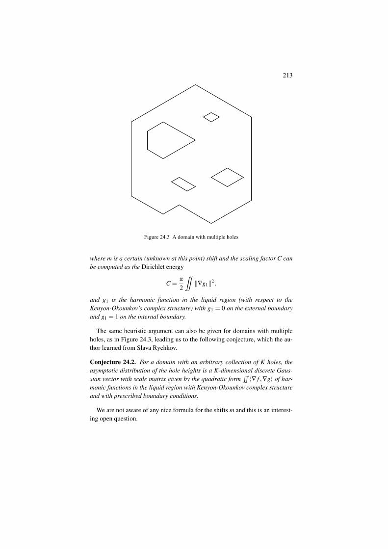
213
Figure 24.3 A domain with multiple holes
where m is a certain (unknown at this point) shift and the scaling factor C canbe computed as the Dirichlet energy
C =π
2
¨‖∇g1‖2,
and g1 is the harmonic function in the liquid region (with respect to theKenyon-Okounkov’s complex structure) with g1 = 0 on the external boundaryand g1 = 1 on the internal boundary.
The same heuristic argument can also be given for domains with multipleholes, as in Figure 24.3, leading us to the following conjecture, which the au-thor learned from Slava Rychkov.
Conjecture 24.2. For a domain with an arbitrary collection of K holes, theasymptotic distribution of the hole heights is a K-dimensional discrete Gaus-sian vector with scale matrix given by the quadratic form
˜〈∇ f ,∇g〉 of har-
monic functions in the liquid region with Kenyon-Okounkov complex structureand with prescribed boundary conditions.
We are not aware of any nice formula for the shifts m and this is an interest-ing open question.
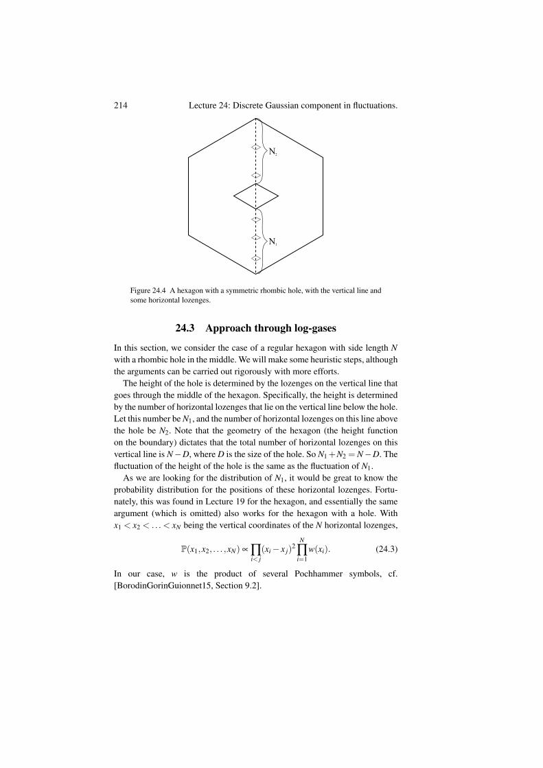
214 Lecture 24: Discrete Gaussian component in fluctuations.
N1
N2
Figure 24.4 A hexagon with a symmetric rhombic hole, with the vertical line andsome horizontal lozenges.
24.3 Approach through log-gases
In this section, we consider the case of a regular hexagon with side length Nwith a rhombic hole in the middle. We will make some heuristic steps, althoughthe arguments can be carried out rigorously with more efforts.
The height of the hole is determined by the lozenges on the vertical line thatgoes through the middle of the hexagon. Specifically, the height is determinedby the number of horizontal lozenges that lie on the vertical line below the hole.Let this number be N1, and the number of horizontal lozenges on this line abovethe hole be N2. Note that the geometry of the hexagon (the height functionon the boundary) dictates that the total number of horizontal lozenges on thisvertical line is N−D, where D is the size of the hole. So N1+N2 = N−D. Thefluctuation of the height of the hole is the same as the fluctuation of N1.
As we are looking for the distribution of N1, it would be great to know theprobability distribution for the positions of these horizontal lozenges. Fortu-nately, this was found in Lecture 19 for the hexagon, and essentially the sameargument (which is omitted) also works for the hexagon with a hole. Withx1 < x2 < .. . < xN being the vertical coordinates of the N horizontal lozenges,
P(x1,x2, . . . ,xN) ∝ ∏i< j
(xi− x j)2
N
∏i=1
w(xi). (24.3)
In our case, w is the product of several Pochhammer symbols, cf.[BorodinGorinGuionnet15, Section 9.2].
215
Exercise 24.3. Extending the argument which produced (19.1), compute wexplicitly.
Now, let us define a ’potential’ V by
w(x) = exp(−NV
( xN
)).
Given a position vector xxx = (x1,x2, . . . ,xN), we also define the following prob-ability measure:
µN =1N
N
∑i=1
δxi/N . (24.4)
As xxx is a random variable, µN is a random distribution. In the limit N→∞, µN
becomes a continuous probability measure. With this notation, we can rewrite
P(xxx) ∝ exp(N2I[µN ]
),
where
I[µN ] =
¨x 6=y
log |x− y|µN(dx)µN(dy)−ˆ
V (x)µN(dx).
As N → ∞, the measure µN concentrates near the maximizer of I[·] —this is another face of the limit shape theorem for random tilings, cf.[BorodinGorinGuionnet15].
Letting µ be the probability distribution that maximizes I[·], we can con-sider a deviation 1
N gN from the maximum (here, 1N gN is the difference of two
probability measures, i.e. has total mass 0), and expand:
I[µN ] = I[µ +1N
gN ] = I[µ]
+1N
(2¨
log |x− y|µ(dy)gN(dx)−ˆ
V (x)gN(dx))
+1
N2 log |x− y|gN(dx)gN(dy).
Since µ is a maximizer and the middle term is a derivative of I[·] at µ (in thegN direction), it is 0. So plugging back into the equation for P(xxx), we get thefollowing proposition.
Proposition 24.4. The law of fluctuations gN as N→ ∞ becomes
P(gN) ∝ exp(¨
log |x− y|gN(dx)gN(dy)).
This is an exponential of a quadratic integral, so we get a Gaussian law.
216 Lecture 24: Discrete Gaussian component in fluctuations.
The above proposition can be proved rigorously using loop(Nekrasov) equations of Lecture 21, see [BorodinGorinGuionnet15] and[BorotGuionnet11], [Johansson98] for a continuous space version.
We now understand the distribution of the fluctuations gN . Note that thesupport of gN is the part of the line that is in the liquid regions, i.e. a pairof intervals [a,b]∪ [c,d], as in Figure 24.5. We would like to also understandthe fluctuation of the height of the hole, which is equal to the fluctuation ofgN [a,b] =−gN [c,d]. The distribution of the latter is
P(gN [a,b] =−gN [c,d] = δ ) ∝
ˆΩδ
exp(¨
log |x− y|gN(dx)gN(dy)).
(24.5)Here, Ωδ is the subset of all gN with gN [a,b] =−gN [c,d] = δ .
Lemma 24.5. The expression in (24.5) is the same as
P(gN [a,b] =−gN [c,d] = δ )
∝ exp(
maxgN such that gN [a,b]=δ
¨log |x− y|gN(dx)gN(dy)
)= exp
(¨log |x− y|gδ (dx)gδ (dy)
),
where gδ is defined to be the maximizer.
Proof This is a general statement about Gaussian vectors, which we leaveas an exercise: the density of projection of a large–dimensional vector onto asmaller subspace can be found through the maximization procedure.
In analogy with the argument from before, we again have gδ = δg1, so weconclude with the following result.
Conjecture 24.6. The height of a hole is asymptotically a discrete Gaussian(integer-valued) random variable, i.e. it has distribution
const · exp(−C(H−m)2),
where m is a certain shift and the scale parameter C is given by the extremumof the logarithmic energy:
C =−max¨
log |x− y|gN(dx)gN(dy),
with the maximum taken over all gN on [a,b]∪ [c,d] gN [a,b] = 1, gN [c,d] =−1.
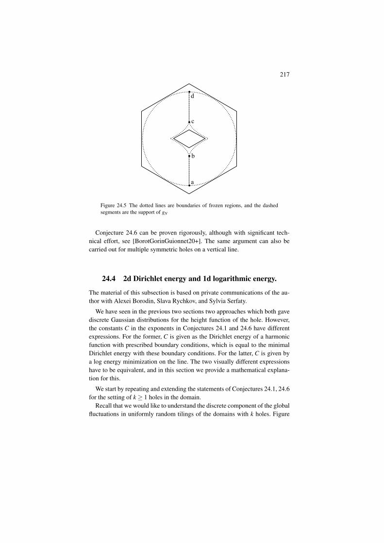
217
a
b
c
d
Figure 24.5 The dotted lines are boundaries of frozen regions, and the dashedsegments are the support of gN
Conjecture 24.6 can be proven rigorously, although with significant tech-nical effort, see [BorotGorinGuionnet20+]. The same argument can also becarried out for multiple symmetric holes on a vertical line.
24.4 2d Dirichlet energy and 1d logarithmic energy.
The material of this subsection is based on private communications of the au-thor with Alexei Borodin, Slava Rychkov, and Sylvia Serfaty.
We have seen in the previous two sections two approaches which both gavediscrete Gaussian distributions for the height function of the hole. However,the constants C in the exponents in Conjectures 24.1 and 24.6 have differentexpressions. For the former, C is given as the Dirichlet energy of a harmonicfunction with prescribed boundary conditions, which is equal to the minimalDirichlet energy with these boundary conditions. For the latter, C is given bya log energy minimization on the line. The two visually different expressionshave to be equivalent, and in this section we provide a mathematical explana-tion for this.
We start by repeating and extending the statements of Conjectures 24.1, 24.6for the setting of k ≥ 1 holes in the domain.
Recall that we would like to understand the discrete component of the globalfluctuations in uniformly random tilings of the domains with k holes. Figure
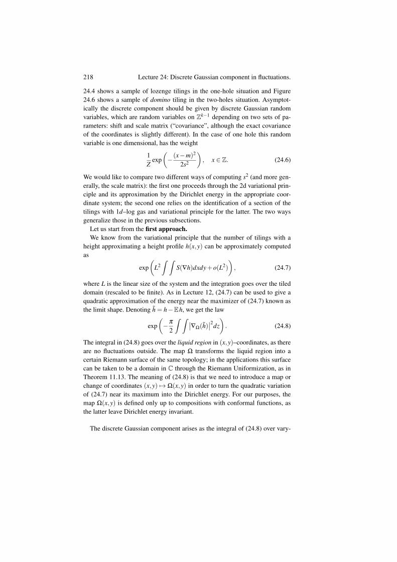
218 Lecture 24: Discrete Gaussian component in fluctuations.
24.4 shows a sample of lozenge tilings in the one-hole situation and Figure24.6 shows a sample of domino tiling in the two-holes situation. Asymptot-ically the discrete component should be given by discrete Gaussian randomvariables, which are random variables on Zk−1 depending on two sets of pa-rameters: shift and scale matrix (“covariance”, although the exact covarianceof the coordinates is slightly different). In the case of one hole this randomvariable is one dimensional, has the weight
1Z
exp(− (x−m)2
2s2
), x ∈ Z. (24.6)
We would like to compare two different ways of computing s2 (and more gen-erally, the scale matrix): the first one proceeds through the 2d variational prin-ciple and its approximation by the Dirichlet energy in the appropriate coor-dinate system; the second one relies on the identification of a section of thetilings with 1d–log gas and variational principle for the latter. The two waysgeneralize those in the previous subsections.
Let us start from the first approach.We know from the variational principle that the number of tilings with a
height approximating a height profile h(x,y) can be approximately computedas
exp(
L2ˆ ˆ
S(∇h)dxdy+o(L2)
), (24.7)
where L is the linear size of the system and the integration goes over the tileddomain (rescaled to be finite). As in Lecture 12, (24.7) can be used to give aquadratic approximation of the energy near the maximizer of (24.7) known asthe limit shape. Denoting h = h−Eh, we get the law
exp(−π
2
ˆ ˆ ∣∣∇Ω(h)∣∣2dz
). (24.8)
The integral in (24.8) goes over the liquid region in (x,y)–coordinates, as thereare no fluctuations outside. The map Ω transforms the liquid region into acertain Riemann surface of the same topology; in the applications this surfacecan be taken to be a domain in C through the Riemann Uniformization, as inTheorem 11.13. The meaning of (24.8) is that we need to introduce a map orchange of coordinates (x,y) 7→ Ω(x,y) in order to turn the quadratic variationof (24.7) near its maximum into the Dirichlet energy. For our purposes, themap Ω(x,y) is defined only up to compositions with conformal functions, asthe latter leave Dirichlet energy invariant.
The discrete Gaussian component arises as the integral of (24.8) over vary-
219
ing boundary conditions. A basic property of the Dirichlet energy in a domainis that for the sum of two functions f = u+v, such that v is harmonic in the do-main and u vanishes on the boundary of the domain, the Dirichlet energy of f isthe sum of Dirichlet energies of u and v. Hence, we can identify the integrals of(24.8) with different boundary conditions. Therefore, the scale of the Gaussiancomponent can be now reconstructed through the computation of the Dirichletenergy of the harmonic functions (in the liquid region, in Ω–coordinate) withappropriate boundary conditions reflecting the height differences on differentconnected components of the boundary. E.g. for the holey hexagon of Figure24.4 there are two connected components of the boundary, and therefore, thereare two heights. By recentering, we can assume that the height of the outercomponent is zero and, therefore, only one variable remains.
It is shown in [BufetovGorin17] that for a class of domains (gluing of trape-zoids in the lozenge case and gluings of Aztec rectangles in the domino case)the map Ω(x,y) can be chosen so that it maps the liquid region into the com-plex plane with cuts. For instance, in the holey hexagon case of Figure 24.4,the cuts can be identified with intervals on the vertical symmetry axis on thepicture; their endpoints coincide with intersection of the frozen boundary ofthe liquid region with the symmetry axis, these are [a,b] and [c,d] in Figure24.5. In the Aztec diamond with two holes of Figure 24.6 the cuts are on thehorizontal axis going through the centers of the holes; again end-points of thecuts lie on the frozen boundary.
We thus are led to the problem of finding Dirichlet energy of harmonic func-tions in a domain with cut. Let us now formulate the setting of the last problemin a self-contained form.
Take 2k real numbers a1 < b1 < a2 < · · · < ak < bk. We refer to intervals[ak,bk] as cuts. Let H denote the (open) upper half-plane and H denote thelower half-plane. Set D=H∪ H∪k
i=1 (ak,bk).Fix k real numbers n1, . . . ,nk subject to the condition n1+ · · ·+nk = 0. These
numbers are fluctuations of the height function in the setting of the previoustext: they are increments of the height as we cross a connected component ofthe liquid region (cf. N1 and N2 in Figure 24.4) with subtracted expectations.The zero sum condition corresponds to the deterministic full increment of theheight function between the points of the outer boundary. In particular, k = 2in Figure 24.4 and k = 3 in Figure 24.6.
We consider continuous functions h(z), z = x+ iy, in C, differentiable in D,
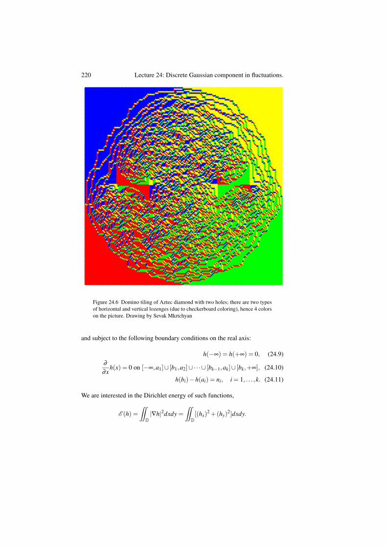
220 Lecture 24: Discrete Gaussian component in fluctuations.
Figure 24.6 Domino tiling of Aztec diamond with two holes; there are two typesof horizontal and vertical lozenges (due to checkerboard coloring), hence 4 colorson the picture. Drawing by Sevak Mkrtchyan
and subject to the following boundary conditions on the real axis:
h(−∞) = h(+∞) = 0, (24.9)∂
∂xh(x) = 0 on [−∞,a1]∪ [b1,a2]∪·· ·∪ [bk−1,ak]∪ [bk,+∞], (24.10)
h(bi)−h(ai) = ni, i = 1, . . . ,k. (24.11)
We are interested in the Dirichlet energy of such functions,
E (h) =¨
D|∇h|2dxdy =
¨D[(hx)
2 +(hy)2]dxdy.
221
We further define a quadratic form C through
C : (n1, . . . ,nk)→π
2min
hE (h), subject to (24.9), (24.10), (24.11). (24.12)
Note that by the Dirichlet principle, the minimizer in (24.12) is a harmonicfunction in D.
Claim 24.7. The quadratic form C is precisely the quadratic form for the dis-crete Gaussian component of the fluctuations of the height function in randomtilings in Conjecture 24.1.
From the second perspective, we saw in the previous section that the sec-tion of a random tiling along a singled out axis gives rise to a discrete log-gas. This axis is the vertical symmetry axis in Figures 24.2, 24.4 and hor-izontal axis going through the centers of the holes in Figure 24.6. Otherexamples can be found in [BorodinGorinGuionnet15], [BufetovGorin17],[BorotGorinGuionnet20+]. Clearly, it is enough to study what is happeningon such axis in order to find the desired discrete Gaussian component of thefluctuation.
In more details, in Figure 24.4 the distribution of the green lozenges onthe vertical section of the tiling by the symmetry axis of the domain has theform of the log-gas. The particles xi in (24.3) belong to two segments – belowand above the hole. We are, thus, interested in fluctuations of the number ofparticles in one of the segments. For a large class of tilings we will have ageneralisation of (24.3) with particles now confined to k segments instead of 2.
If we denote through µN the empirical measure of the particles as in (24.4),then (24.3) can rewritten (ignoring the diagonal) as
exp[
N2(¨
ln |x− y|µN(dx)µN(dy)+ˆ
lnw(Nx)µ(dx))]
(24.13)
The maximizer of the functional in the exponent of (24.13) is the equilib-rium measure. The fluctuations of the numbers of particles (called fillingfractions in this context) can be thus obtained by varying this functionalnear its extremum. Rigorous justification of this procedure is the subject or[BorotGorinGuionnet20+]. In the continuous setting (when xi in (24.3) are realnumbers rather than integers), the detailed rigorous analysis for arbitrary num-ber of cuts k was done in [BorotGuionnet11].
Let us describe how the approximation of the functional near the equilibriummeasure looks like. We assume that the bands of the equilibrium measure are kintervals [a1,b1],. . . , [ak,bk]. Recall that bands are regions where the density is
222 Lecture 24: Discrete Gaussian component in fluctuations.
not 0 and not 1s as in the liquid region for tilings (i.e. not frozen/saturated, thelatter corresponding to the areas in Figure 24.4 densely packed with particles).
Given n1, . . . ,nk with n1 + · · ·+ nk = 0, we are led to consider signed mea-sures ν on the union of the intervals [ai,bi] subject to filling fractions:
ν([ai,bi]) = ni, i = 1, . . . ,k. (24.14)
We consider the logarithmic energy of such measure given by
E =−ˆ ˆ
ln |x− y|ν(dx)ν(dy). (24.15)
Define a quadratic functional C through
C : (n1, . . . ,nk)→minν
E (ν) subject to (24.14). (24.16)
Claim 24.8. The quadratic form C is precisely the quadratic form for the dis-crete Gaussian component of the fluctuations of the height function in randomtilings, as in Conjecture 24.6.
Of course, both Claim 24.7 and Claim 24.8 describe the same object.The advantage of Claim 24.8 is that we are actually able to prove it in[BorotGorinGuionnet20+]. Nevertheless, the answers in these claims also lookvisually different. Hence, we are led to proving the following statement.
Proposition 24.9. Quadratic forms (24.12) and (24.16) are the same.
Proof The key idea is to split the minimization procedure in (24.12) into twosteps. First, we will fix the values of h on the real axis in arbitrary way subjectto (24.9), (24.10), (24.11) and minimize over all such functions. The minimizeris then a harmonic function separately in the upper half–plane and in the lowerhalf–plane; by symmetry, the values differ by conjugation of the arguments.By the Schwarz integral formula (i.e. Poisson kernel), this harmonic functioncan be expressed as an integral over the real axis
h(z) = ℜ
[1πi
ˆ∞
−∞
h(ζ )ζ − z
dζ
], z ∈H, (24.17)
and by a similar expression with changed sign in the lower halfplane H.In the second step we minimize the Dirichlet energy over the choices of the
values of h on the real axis. We claim that the latter optimization is the sameas the log-energy optimization of (24.16). Let us explain this.
We identify a function on the real axis h(x) with a signed measure ν throughh(y)−h(x)= ν([x,y]). Although, a priori the functions do not have to be differ-entiable and the signed measures do not have to be absolutely continuous, how-ever, the minimum in (24.12) and (24.16) is attained on differentiable functions
223
and measures with densities, respectively. Thus, we can restrict ourselves to thelatter, in which case the derivative hx(x) becomes the density of ν . Clearly, un-der such identification, conditions on h (24.9)-(24.11) become conditions on ν
(24.14). It thus remains to show that the functional (24.12) turns into (24.16).Let us compute the Dirichlet energy of h(x + iy) given by (24.17) in the
domain y≥ ε > 0. Integrating by parts, we get¨
y≥ε
[(hx)
2 +(hy)2]dxdy
=
ˆ +∞
ε
dy[(hhx)(+∞+ iy)− (hhx)(−∞+ iy)−
ˆ∞
−∞
hhxxdx]
+
ˆ∞
−∞
dx[(hhy)(x+ i∞)− (hhy)(x+ iε)−
ˆ∞
ε
hhyydy]. (24.18)
Further, note that since h(x) has a compact support on the real axis, h(z)given by (24.17) decays as O(1/|z|) when z→ ∞ and its derivatives decayas O(1/|z|2). Hence, all the boundary terms at the infinity in (24.18) vanish.Moreover, since h is harmonic, hhxx+hhyy = 0 and the double integral vanishesas well. We conclude that (24.18) is
−ˆ
∞
−∞
(hhy)(x+ iε)dx =−ˆ
∞
−∞
dxh(x+ iε)ℜ[
1π
ˆ∞
−∞
h(ζ )−(ζ − (x+ iε))2 dζ
]We integrate by parts both in x and in ζ to get
− 1π
ˆ∞
−∞
dxhx(x+ iε)ℜ[ˆ
∞
−∞
hx(ζ ) ln(ζ − (x+ iε))dζ
].
Note that we need to choose some branch of the logarithm here, but it does notmatter, as we will get the logarithm of the absolute value when computing thereal part anyway.
At this point it remains to send ε → 0 (As the integrand is singular and wealso have hx rather than h itself, this needs some justifications, which we omit),and to add the same contribution from the lower half-plane to get the desired
¨D|∇h|2dxdy =− 2
π
ˆ∞
−∞
ˆ∞
−∞
hx(x)hx(ζ ) ln |ζ − x|dxdζ ,
which matches (24.16).
Remark 24.10. Although we were only concentrating on the discrete compo-nent, but essentially the same arguments explain the link between covariancestructures for the entire field of fluctuations: Gaussian Free Field in the 2d pic-ture and universal covariance of random matrix theory and log-gases on the 1d
224 Lecture 24: Discrete Gaussian component in fluctuations.
section. This covariance coincidence is also discussed (through other tools) in[BufetovGorin17], [BorodinGorinGuionnet15].
Remark 24.11. It is interesting to also try to do similar identification for theshifts — m in (24.6). This involves computing the second order expansion ofthe logarithm of the partition function — we need O(N) rather than O(N2)
terms. On the side of log-gases there is a certain understanding of how this canbe done (at least for continuous log–gases). On the other hand, the author is notaware of approaches to the computation of this second term in the 2d settingof random tilings.
24.5 Discrete component in tilings on Riemann surfaces
There is another natural situation in which the height function of lozengetilings asymptotically develops a discrete Gaussian component.
Let us give an example by looking at lozenge tilings of a torus, as we didin Lectures 3, 4, and 6. The height function does not make sense on torus as asingle-valued function: we define the heights by local rules and typically theserules result in a non-trivial increment as we loop around the torus and comeback to the same point.
There are two closely related ways to deal with this difficulty. We couldeither split the height function into two components: affine multivalued part(sometimes called the instanton part) keeping track of the height change as weloop around the torus, and a scalar single-valued part. Alternatively, we candefine the height function as a 1–form, so that it is a not function of the point,but rather of a path on the torus, and therefore is allowed to have differentvalues on paths representing different homotopy classes. In both ways, onecan single out the component which asymptotically converges to a discreteGaussian random variable: in the first approach this is the instanton part, andin the second approach these are the values of the 1–form on closed loops.
More generally, a similar component can be singled out whenever we dealwith tilings of domains embedded into Riemann surfaces of higher genus. Wedeal with random functions of homotopy classes of closed loops and we canask about the asymptotic of such functions as the mesh size goes to 0.
In several situations the convergence of the discrete component of thetilings on Riemann surfaces to discrete Gaussian random variables was rig-orously proved, see [BoutillierDeTiliere06, Dubedat11, KenyonSunWilson13,DubedatGheissari14, BerestyckiLaslierRay19].
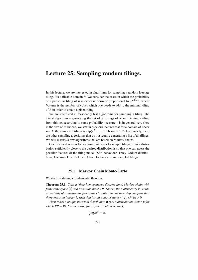
Lecture 25: Sampling random tilings.
In this lecture, we are interested in algorithms for sampling a random lozengetiling. Fix a tileable domain R. We consider the cases in which the probabilityof a particular tiling of R is either uniform or proportional to qVolume, whereVolume is the number of cubes which one needs to add to the minimal tilingof R in order to obtain a given tiling.
We are interested in reasonably fast algorithms for sampling a tiling. Thetrivial algorithm – generating the set of all tilings of R and picking a tilingfrom this set according to some probability measure – is in general very slowin the size of R. Indeed, we saw in previous lectures that for a domain of linearsize L, the number of tilings is exp(L2 . . .), cf. Theorem 5.15. Fortunately, thereare other sampling algorithms that do not require generating a list of all tilings.We will discuss a few algorithms that are based on Markov chains.
One practical reason for wanting fast ways to sample tilings from a distri-bution sufficiently close to the desired distribution is so that one can guess thepeculiar features of the tiling model (L1/3 behaviour, Tracy-Widom distribu-tions, Gaussian Free Field, etc.) from looking at some sampled tilings.
25.1 Markov Chain Monte-Carlo
We start by stating a fundamental theorem.
Theorem 25.1. Take a (time-homogeneous discrete time) Markov chain withfinite state space [n] and transition matrix P. That is, the matrix entry Pi j is theprobability of transitioning from state i to state j in one time step. Suppose thatthere exists an integer k, such that for all pairs of states (i, j), (Pk)i j > 0.
Then P has a unique invariant distribution πππ (i.e. a distribution vector πππ forwhich πππP = πππ). Furthermore, for any distribution vector xxx,
limt→∞
xxxPt = πππ.
225
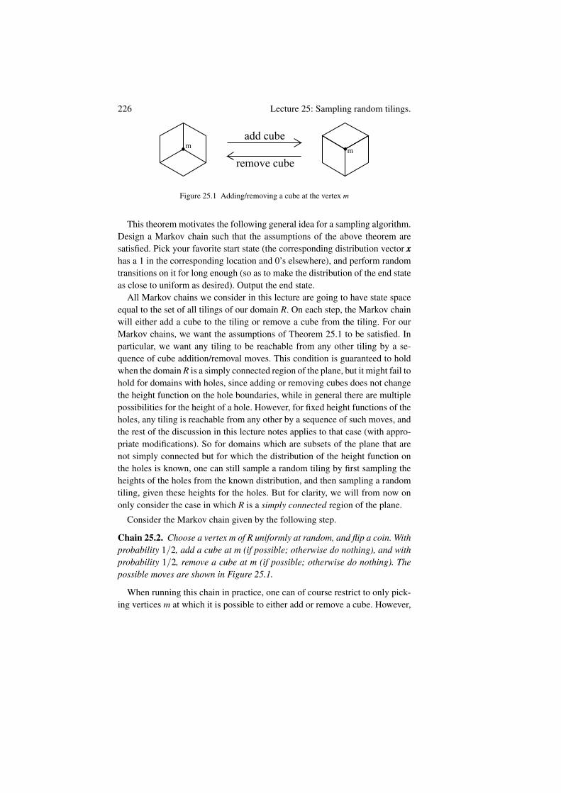
226 Lecture 25: Sampling random tilings.
add cube
remove cube
mm
Figure 25.1 Adding/removing a cube at the vertex m
This theorem motivates the following general idea for a sampling algorithm.Design a Markov chain such that the assumptions of the above theorem aresatisfied. Pick your favorite start state (the corresponding distribution vector xxxhas a 1 in the corresponding location and 0’s elsewhere), and perform randomtransitions on it for long enough (so as to make the distribution of the end stateas close to uniform as desired). Output the end state.
All Markov chains we consider in this lecture are going to have state spaceequal to the set of all tilings of our domain R. On each step, the Markov chainwill either add a cube to the tiling or remove a cube from the tiling. For ourMarkov chains, we want the assumptions of Theorem 25.1 to be satisfied. Inparticular, we want any tiling to be reachable from any other tiling by a se-quence of cube addition/removal moves. This condition is guaranteed to holdwhen the domain R is a simply connected region of the plane, but it might fail tohold for domains with holes, since adding or removing cubes does not changethe height function on the hole boundaries, while in general there are multiplepossibilities for the height of a hole. However, for fixed height functions of theholes, any tiling is reachable from any other by a sequence of such moves, andthe rest of the discussion in this lecture notes applies to that case (with appro-priate modifications). So for domains which are subsets of the plane that arenot simply connected but for which the distribution of the height function onthe holes is known, one can still sample a random tiling by first sampling theheights of the holes from the known distribution, and then sampling a randomtiling, given these heights for the holes. But for clarity, we will from now ononly consider the case in which R is a simply connected region of the plane.
Consider the Markov chain given by the following step.
Chain 25.2. Choose a vertex m of R uniformly at random, and flip a coin. Withprobability 1/2, add a cube at m (if possible; otherwise do nothing), and withprobability 1/2, remove a cube at m (if possible; otherwise do nothing). Thepossible moves are shown in Figure 25.1.
When running this chain in practice, one can of course restrict to only pick-ing vertices m at which it is possible to either add or remove a cube. However,
227
the above formulation is what we will use formally, because it has a numberof nice properties. Note that Chain 25.2 satisfies the assumption of Theorem25.1, as any tiling can be reached from any other and there is always a nonzeroprobability of not changing the tiling, from which the assumption of the theo-rem follows. Hence, this chain has a unique invariant distribution, and we havethe following proposition.
Proposition 25.3. The uniform distribution is the invariant distribution ofChain 25.2.
Proof For a general Markov chain, to show that πππ is an invariant distribution,it suffices to show reversibility, that is πiPi j = π jPji. Indeed, if this holds, then
(πππP) j = ∑i
πiPi j = ∑i
π jPji = π j ∑i
Pji = π j =⇒ πππP = πππ.
So it remains to show that for our cube switching Markov chain, πππ = the uni-form distribution satisfies πiPi j = π jPji. This is just a case check:
1 If i = j, then this is trivially true.2 If tilings i and j are different, but do not differ by adding/removing a single
cube, then Pi j = Pji = 0, so we are done.3 If tilings i and j differ by adding/removing a single cube, then both Pi j and
Pji are 12 ·
1number of vertices , so we are done since for the uniform distribution
πi = π j. Note that it is crucial here that our Markov chain step involvespicking a random vertex regardless of whether a cube flip can be performedthere.
As for the qVolume distribution, consider the following Markov chain that isthe same as Chain 25.2, except with different probabilities for adding/removingcubes.
Chain 25.4. Choose a vertex m of R uniformly at random, and flip a biasedcoin. With probability q
1+q , add a cube at m (if possible; otherwise do noth-ing), and with probability 1
1+q , remove a cube at m (if possible; otherwise donothing).
As argued before, Chain 25.4 also has a unique invariant distribution. Wehave the following proposition.
Proposition 25.5. The qVolume distribution is the invariant distribution ofChain 25.4.
Proof As argued before, it suffices to show reversibility, i.e. that πiPi j = π jPji.This is just a case check:
228 Lecture 25: Sampling random tilings.
1 If i = j, then this is trivially true.
2 If tilings i and j are different but do not differ by adding/removing a singlecube, then Pi j = Pji = 0, so we are done.
3 If tilings i and j differ by adding/removing a single cube, with WLOG tilingj having 1 cube more than tiling i, then for the qVolume distribution πππ , π j
πi= q,
and with our transition probabilities, Pi jPji
=q
1+q1
1+q= q. The desired equality
πiPi j = π jPji follows.
So we have the following algorithm for sampling a random tiling.
Algorithm 25.6. Pick your favorite tiling. Run either Chain 25.2 (for the uni-form distribution) or Chain 25.4 (for the qVolume distribution) long enough, andoutput the result.
Of course, this does not give exactly the distribution we are interested infor any finite time, but by Theorem 25.1, as the time goes to infinity, it givesan arbitrarily good approximation. One may ask what the runtime should befor the approximation to be ’sufficiently good’. To be more rigorous, definethe total variation distance between two distributions µ1,µ2 on a finite spaceX to be ∑x∈X |µ1(x)− µ2(x)|. Define the mixing time of this Markov chainto be the minimal amount of time t the above algorithm needs to run (fromany start state), so that for all t ′ ≥ t, the variation distance between the in-duced distribution and the desired distribution is at most some fixed constantε . In [RandallTetali00] an upper bound O(L8 lnL) for the mixing time in thedomain of linear size L was obtained. For a slightly different Markov chain(which allows addition/removal of 1×1× k stacks of cubes; it was introducedin [LubyRandallSinclair95]), the mixing time was shown to be O(L4 lnL)in [Wilson01] and for hexagons this bound is tight up to a constant factor.[Wilson01, Section 5.6] discusses that the mixing time for our chain (addingonly one cube at a time) is expected to be of the same order for “good” do-mains. This prediction (which also agrees with expectations from the the-oretical physics literature) matches more recent results on the mixing timefor our chain in specific classes of domains [CaputoMartinelliToninelli11],[LaslierToninelli13].
A general behaviour (cf. [LevinPeresWilmer17]) is that before some timethe chain is not mixed at all, and after that time it is mixed very well. To getan idea of what the above estimates mean in practice, for instance, when ourdomain is a hexagon of side length 1000, one should run the Markov chain ona personal computer for about an entire day to get a good approximation.
229
25.2 Coupling from the past [ProppWilson96]
In any finite amount of time, the previous algorithm only gives a sample froman approximation of the desired distribution. This is often inconvenient, aswe would like to look at very delicate features of the tilings, and therefore,knowing that our sample is exact rather than approximate becomes important.With an ungrade known as coupling from the past, we can sample from thedesired distribution without any error.
Let us first discuss some ideas that will eventually lead us to the couplingfrom the past algorithm. Suppose we can run our Markov chain in a coupledway from all states, i.e. picking a sequence of transitions (which we think ofas transitions from any state via some canonical identification, and not justtransitions from some fixed state) and applying this same sequence to all startstates. Further suppose that at some time t, we notice that we have reached thesame final state from all start states. Suppose we output this final state. Sincethis state is independent from the initial configuration, one might expect that itis a sample from the invariant distribution, as we can imagine starting from theinvariant distribution originally. However, there are a few issues here.
First, with the algorithm as stated, we still run into our original problem – thetotal number of states is huge, so it would take a huge amount of time to simul-taneously run this procedure from all start states. It turns out that this problemcan be fixed, due to the fact that transitions preserve the height poset structureon tilings. This will be explained in more detail in the next few paragraphs.
The second issue is that there is no way to choose the desired time t deter-ministically, while if t is random (e.g. we choose it as the first time when allinitial states lead to the same current state), then it becomes unclear whetherthe distribution of the output of such an algorithm is the invariant distributionof the Markov chain. Unfortunately, this turns out to be false in general, as thefollowing counterexample shows. Suppose we have a Markov chain that satis-fies the assumptions of Theorem 25.1 with more than one state, and with a stateinto which one can transition from exactly one state (also counting the state it-self). It is not hard to see that such Markov chains exist. Then the probability ofoutputting this state at first time t is clearly 0. However, (under assumptions ofTheorem 25.1), the invariant distribution can not assign 0 probability to somestate. So the distribution of the output of our algorithm is not the invariantdistribution.
Let us first explain how to work around the issue of not being able to run theMarkov chain from all initial states.
Proposition 25.7. Suppose we have two tilings A0 and B0, such that at each
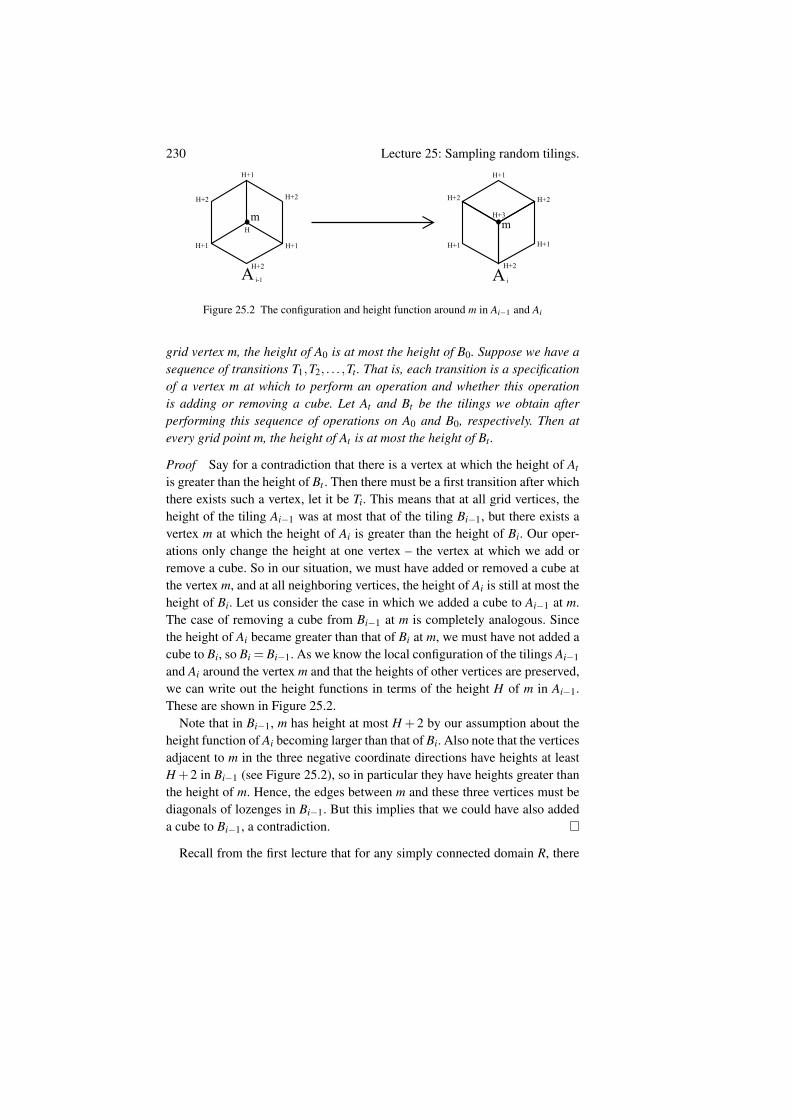
230 Lecture 25: Sampling random tilings.
mm
Ai-1 Ai
H
H+1
H+2 H+2 H+2 H+2
H+2
H+1
H+1 H+1
H+1H+1
H+2
H+3
Figure 25.2 The configuration and height function around m in Ai−1 and Ai
grid vertex m, the height of A0 is at most the height of B0. Suppose we have asequence of transitions T1,T2, . . . ,Tt . That is, each transition is a specificationof a vertex m at which to perform an operation and whether this operationis adding or removing a cube. Let At and Bt be the tilings we obtain afterperforming this sequence of operations on A0 and B0, respectively. Then atevery grid point m, the height of At is at most the height of Bt .
Proof Say for a contradiction that there is a vertex at which the height of At
is greater than the height of Bt . Then there must be a first transition after whichthere exists such a vertex, let it be Ti. This means that at all grid vertices, theheight of the tiling Ai−1 was at most that of the tiling Bi−1, but there exists avertex m at which the height of Ai is greater than the height of Bi. Our oper-ations only change the height at one vertex – the vertex at which we add orremove a cube. So in our situation, we must have added or removed a cube atthe vertex m, and at all neighboring vertices, the height of Ai is still at most theheight of Bi. Let us consider the case in which we added a cube to Ai−1 at m.The case of removing a cube from Bi−1 at m is completely analogous. Sincethe height of Ai became greater than that of Bi at m, we must have not added acube to Bi, so Bi = Bi−1. As we know the local configuration of the tilings Ai−1
and Ai around the vertex m and that the heights of other vertices are preserved,we can write out the height functions in terms of the height H of m in Ai−1.These are shown in Figure 25.2.
Note that in Bi−1, m has height at most H + 2 by our assumption about theheight function of Ai becoming larger than that of Bi. Also note that the verticesadjacent to m in the three negative coordinate directions have heights at leastH +2 in Bi−1 (see Figure 25.2), so in particular they have heights greater thanthe height of m. Hence, the edges between m and these three vertices must bediagonals of lozenges in Bi−1. But this implies that we could have also addeda cube to Bi−1, a contradiction.
Recall from the first lecture that for any simply connected domain R, there
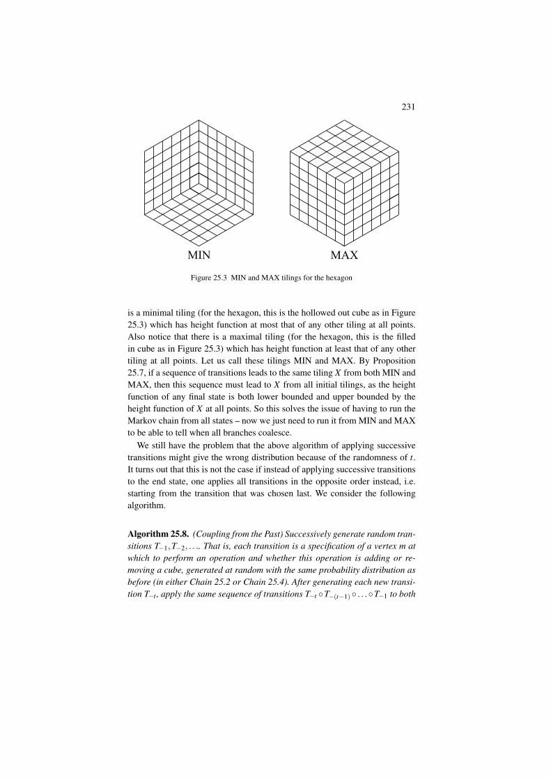
231
MIN MAX
Figure 25.3 MIN and MAX tilings for the hexagon
is a minimal tiling (for the hexagon, this is the hollowed out cube as in Figure25.3) which has height function at most that of any other tiling at all points.Also notice that there is a maximal tiling (for the hexagon, this is the filledin cube as in Figure 25.3) which has height function at least that of any othertiling at all points. Let us call these tilings MIN and MAX. By Proposition25.7, if a sequence of transitions leads to the same tiling X from both MIN andMAX, then this sequence must lead to X from all initial tilings, as the heightfunction of any final state is both lower bounded and upper bounded by theheight function of X at all points. So this solves the issue of having to run theMarkov chain from all states – now we just need to run it from MIN and MAXto be able to tell when all branches coalesce.
We still have the problem that the above algorithm of applying successivetransitions might give the wrong distribution because of the randomness of t.It turns out that this is not the case if instead of applying successive transitionsto the end state, one applies all transitions in the opposite order instead, i.e.starting from the transition that was chosen last. We consider the followingalgorithm.
Algorithm 25.8. (Coupling from the Past) Successively generate random tran-sitions T−1,T−2, . . .. That is, each transition is a specification of a vertex m atwhich to perform an operation and whether this operation is adding or re-moving a cube, generated at random with the same probability distribution asbefore (in either Chain 25.2 or Chain 25.4). After generating each new transi-tion T−t , apply the same sequence of transitions T−t T−(t−1) . . .T−1 to both
232 Lecture 25: Sampling random tilings.
MIN and MAX. If the two tilings obtained from both start states are the same,output this tiling (and halt).
In practice, it is more efficient to only apply the transitions to MIN and MAXafter generating t = 1,2,4,8, . . . of them. It is easy to see that this algorithmhalts almost surely. Let us now prove that this algorithm generates samplesfrom exactly the desired distribution.
Proposition 25.9. The distribution of the output of Algorithm 25.8 is preciselythe invariant distribution of the corresponding tiling Markov chain (uniformor qVolume).
Proof If T−t T−(t−1) . . . T−1 takes both MIN and MAX to the same endstate i, then it also does so for any other state (as explained before). Thecrucial observation is that if T−t T−(t−1) . . . T−1 takes all initial states toi, then for t ′ > t, T−t ′ T−(t ′−1) . . . T−1 =
(T−t ′ T−(t ′−1) . . .T−(t+1)
)(
T−t T−(t ′−1) . . .T−1)
also takes any initial state to i. Starting from any startstate (i.e. a distribution vector xxx with a 1 in the corresponding location and 0’selsewhere), Theorem 25.1 gives that xxxPt approaches the invariant distributionas t → ∞. Since for any particular sequence of transitions . . . ,T−2,T−1, therealmost surely exists a time t after which the end state is unchanged by addingtransitions to the beginning, the limiting distribution (formally, the limitingdistribution starting from some fixed start state – although it does not matter,as the result is the same for all start states) is also equal to the distribution ofthe end states generated by our algorithm. Hence, the distribution of these endstates is equal to the invariant distribution of the Markov chain. This is whatwe wanted to show.
To recap, one advantage Algorithm 25.8 has is that it allows sampling fromthe exact distribution we desire, whereas the simple Markov chain Monte-Carlo algorithm considered before only samples from a good approximationof this distribution. The runtime is unbounded, but the algorithm almost surelystops in finite time. For the hexagon, the expected runtime is of the same orderas the mixing time. Coupling from the past is also useful for sampling fromother large systems, e.g. the six-vertex model.
Although coupling from the past is a powerful and simple to implementmethod, it is by no means a unique way to sample random tilings. In the nextsections we briefly mention other approaches.
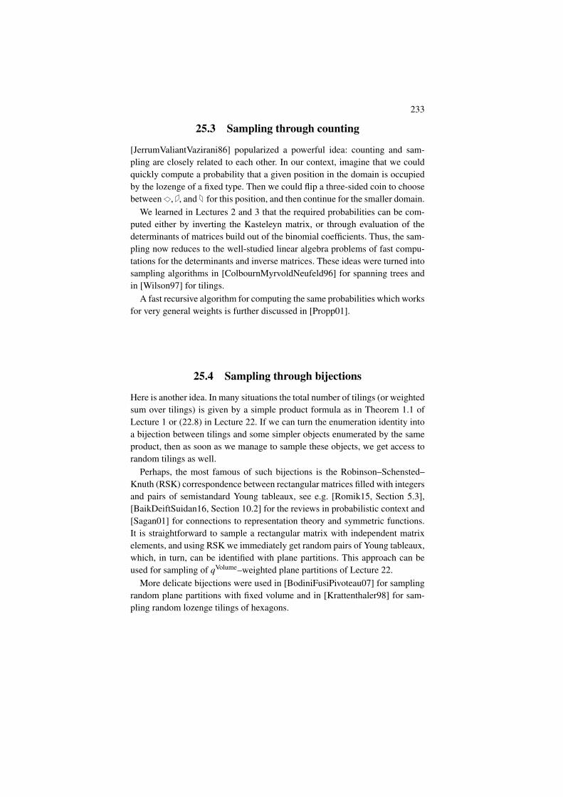
233
25.3 Sampling through counting
[JerrumValiantVazirani86] popularized a powerful idea: counting and sam-pling are closely related to each other. In our context, imagine that we couldquickly compute a probability that a given position in the domain is occupiedby the lozenge of a fixed type. Then we could flip a three-sided coin to choosebetween , , and for this position, and then continue for the smaller domain.
We learned in Lectures 2 and 3 that the required probabilities can be com-puted either by inverting the Kasteleyn matrix, or through evaluation of thedeterminants of matrices build out of the binomial coefficients. Thus, the sam-pling now reduces to the well-studied linear algebra problems of fast compu-tations for the determinants and inverse matrices. These ideas were turned intosampling algorithms in [ColbournMyrvoldNeufeld96] for spanning trees andin [Wilson97] for tilings.
A fast recursive algorithm for computing the same probabilities which worksfor very general weights is further discussed in [Propp01].
25.4 Sampling through bijections
Here is another idea. In many situations the total number of tilings (or weightedsum over tilings) is given by a simple product formula as in Theorem 1.1 ofLecture 1 or (22.8) in Lecture 22. If we can turn the enumeration identity intoa bijection between tilings and some simpler objects enumerated by the sameproduct, then as soon as we manage to sample these objects, we get access torandom tilings as well.
Perhaps, the most famous of such bijections is the Robinson–Schensted–Knuth (RSK) correspondence between rectangular matrices filled with integersand pairs of semistandard Young tableaux, see e.g. [Romik15, Section 5.3],[BaikDeiftSuidan16, Section 10.2] for the reviews in probabilistic context and[Sagan01] for connections to representation theory and symmetric functions.It is straightforward to sample a rectangular matrix with independent matrixelements, and using RSK we immediately get random pairs of Young tableaux,which, in turn, can be identified with plane partitions. This approach can beused for sampling of qVolume–weighted plane partitions of Lecture 22.
More delicate bijections were used in [BodiniFusiPivoteau07] for samplingrandom plane partitions with fixed volume and in [Krattenthaler98] for sam-pling random lozenge tilings of hexagons.
234 Lecture 25: Sampling random tilings.
25.5 Sampling through transformations of domains
There are specific domains, for which the number of tilings is small and sam-pling is easy. This could be either because the domain itself is very small, orbecause the height function is extremal along the boundary. For instance, theA×B×0 hexagon has a unique tiling.
A central idea for a class of algorithms is to introduce a Markov chain (withlocal transition rules), which takes a uniformly random tiling of a domain asan input and gives a uniformly random tiling of a slightly more complicateddomain as an output. In this way, we can start from a domain with a singletiling and reach much more complicated regions in several steps. The maindifficulty in this approach is to design such a Markov chain, as there is nouniversal recipe to produce it.
The first example of such a chain is known as the shuffling algorithm forthe Aztec diamond [ElkiesKuperbergLarsenPropp92] . It works with tilings ofrhombuses drawn on the square grid (“diamonds”) with 2× 1 dominos, as inFigure 1.10 of Lecture 1. Starting from 2×2 square, which has two tilings, itgrows the size of the domain, ultimately getting to huge rhombuses.
There are several different points of view on the shuffling algorithm whichlead to different generalizations. The first point of view is that it provides astochastic version of a deterministic operation which modifies a bipartite graphthrough a sequence of local moves (known as urban renewal or spider move)with explicitly controlled change of the (weighted) count of all perfect match-ings. It is explained in [Propp01] how this can be used for sampling randomdomino tilings with quite generic weights. Since the admissible weights in thisprocedure are essentially arbitrary, it is is very flexible: by various degener-ations one can get all kinds of complicated domains, tilings on other lattices(including lozenge tilings), etc. Extending beyond the probabilistic context,urban renewal is studied as an abstract algebraic operation on weighted bi-partite graphs in [GoncharovKenyon11]; it was further linked to the Miquelmove on cycle patterns (arrangements of intersecting circles on the plane) in[Affolter18, KenyonLamRamassamyRusskikh18].
Another point of view exploits the connections of the domino tilings toSchur polynomials (which is similar to the lozenge tilings case we saw inProposition 19.3 and Lecture 22, see also [BufetovKnizel16]). Along theselines [Borodin10] constructed an efficient sampler for qVolume-weighted planepartitions which we discussed in Lectures 22-23 and their skew versions.
The third point of view treats domino tilings as orthogonal polyno-mial ensembles, cf. footnote to Exercise 21.7 and see [CohnElkiesPropp96,Johansson05]. Along these lines [BorodinGorin08], [BorodinGorinRains09]
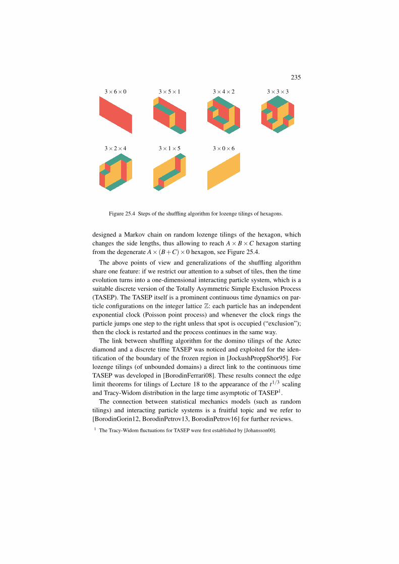
235
3×6×0 3×5×1 3×4×2 3×3×3
3×2×4 3×1×5 3×0×6 empty
Figure 25.4 Steps of the shuffling algorithm for lozenge tilings of hexagons.
designed a Markov chain on random lozenge tilings of the hexagon, whichchanges the side lengths, thus allowing to reach A×B×C hexagon startingfrom the degenerate A× (B+C)×0 hexagon, see Figure 25.4.
The above points of view and generalizations of the shuffling algorithmshare one feature: if we restrict our attention to a subset of tiles, then the timeevolution turns into a one-dimensional interacting particle system, which is asuitable discrete version of the Totally Asymmetric Simple Exclusion Process(TASEP). The TASEP itself is a prominent continuous time dynamics on par-ticle configurations on the integer lattice Z: each particle has an independentexponential clock (Poisson point process) and whenever the clock rings theparticle jumps one step to the right unless that spot is occupied (“exclusion”);then the clock is restarted and the process continues in the same way.
The link between shuffling algorithm for the domino tilings of the Aztecdiamond and a discrete time TASEP was noticed and exploited for the iden-tification of the boundary of the frozen region in [JockushProppShor95]. Forlozenge tilings (of unbounded domains) a direct link to the continuous timeTASEP was developed in [BorodinFerrari08]. These results connect the edgelimit theorems for tilings of Lecture 18 to the appearance of the t1/3 scalingand Tracy-Widom distribution in the large time asymptotic of TASEP1.
The connection between statistical mechanics models (such as randomtilings) and interacting particle systems is a fruitful topic and we refer to[BorodinGorin12, BorodinPetrov13, BorodinPetrov16] for further reviews.1 The Tracy-Widom fluctuations for TASEP were first established by [Johansson00].
References
[AdlerJohanssonMoerbeke16] M. Adler, K. Johansson and P. van Moerbeke, Tilings ofnonconvex Polygons, skew-Young Tableaux and determinantal Processes, Com-munications in Mathematical Physics 364 (2018), 287-342. arXiv:1609.06995
[AdlerJohanssonMoerbeke17] M. Adler, K. Johansson and P. van Moerbeke, Lozengetilings of hexagons with cuts and asymptotic fluctuations: a new universality class,Mathematical Physics, Analysis and Geometry 21 (2018) 1-53. arXiv:1706.01055
[Affolter18] N. C. Affolter, Miquel Dynamics, Clifford Lattices and the Dimer Model.arXiv:1808.04227
[Aggarwal14] A. Aggarwal, Correlation functions of the Schur process through Mac-donald difference operators. Journal of Combinatorial Theory, Series A 131(2015), 88–118. arXiv:1401.6979
[Aggarwal19] A. Aggarwal, Universality for lozenge tilings local statistics.arXiv:1907.09991
[AissenSchoenbergWhitney52] M. Aissen, I. J. Schoenberg, and A. Whitney, Onthe generating functions of totally positive sequences I. Journal d’AnalyseMathematique 2 (1952), 93–103.
[Ahn18] A. Ahn, Global Universality of Macdonald Plane Partitions, to appear in An-nales de l’Institut Henri Poincare. arXiv:1809.02698
[AkemannBaikFrancesco11] G. Akemann, J. Baik, P. Di Francesco (editors), The Ox-ford Handbook of Random Matrix Theory, Oxford University Press, 2011.
[AndersonGuionnetZeitouni10] G. W. Anderson, A. Guionnet, O. Zeitouni, An Intro-duction to Random Matrices, Cambridge University Press, 2010.
[ArdilaStanley05] F. Ardila, R. P. Stanley, Tilings. The Mathematical Intelligencer, 32(2010), 32–43. arXiv:math/0501170
[Azuma67] K. Azuma. Weighted sums of certain dependent random variables. TohokuMathematical Journal, Second Series, 19(3):357–367, 1967
[BaikKriecherbauerMcLaughlinMiller03] J. Baik, T. Kriecherbauer, K. T. -R. McLaughlin, P. D. Miller, Uniform Asymptotics for Polynomials OrthogonalWith Respect to a General Class of Discrete Weights and Universality Results forAssociated Ensembles, International Mathematics Research Notices 2003, no.15. arXiv:math/0310278
[BaikDeiftSuidan16] J. Baik, P. Deift, T. Suidan, Combinatorics and Random MatrixTheory. Graduate studies in Mathematics 172, AMS, Providence, RI, 2016.
[Baryshnikov01] Y. Baryshnikov, GUEs and queues, Probability Theory and RelatedFields, 119, no. 2 (2001), 256–274.
236
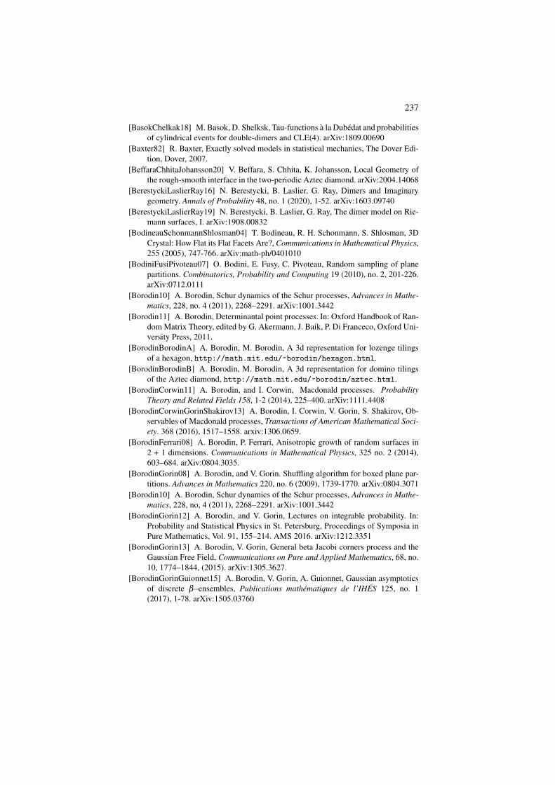
237
[BasokChelkak18] M. Basok, D. Shelksk, Tau-functions a la Dubedat and probabilitiesof cylindrical events for double-dimers and CLE(4). arXiv:1809.00690
[Baxter82] R. Baxter, Exactly solved models in statistical mechanics, The Dover Edi-tion, Dover, 2007.
[BeffaraChhitaJohansson20] V. Beffara, S. Chhita, K. Johansson, Local Geometry ofthe rough-smooth interface in the two-periodic Aztec diamond. arXiv:2004.14068
[BerestyckiLaslierRay16] N. Berestycki, B. Laslier, G. Ray, Dimers and Imaginarygeometry. Annals of Probability 48, no. 1 (2020), 1-52. arXiv:1603.09740
[BerestyckiLaslierRay19] N. Berestycki, B. Laslier, G. Ray, The dimer model on Rie-mann surfaces, I. arXiv:1908.00832
[BodineauSchonmannShlosman04] T. Bodineau, R. H. Schonmann, S. Shlosman, 3DCrystal: How Flat its Flat Facets Are?, Communications in Mathematical Physics,255 (2005), 747-766. arXiv:math-ph/0401010
[BodiniFusiPivoteau07] O. Bodini, E. Fusy, C. Pivoteau, Random sampling of planepartitions. Combinatorics, Probability and Computing 19 (2010), no. 2, 201-226.arXiv:0712.0111
[Borodin10] A. Borodin, Schur dynamics of the Schur processes, Advances in Mathe-matics, 228, no. 4 (2011), 2268–2291. arXiv:1001.3442
[Borodin11] A. Borodin, Determinantal point processes. In: Oxford Handbook of Ran-dom Matrix Theory, edited by G. Akermann, J. Baik, P. Di Franceco, Oxford Uni-versity Press, 2011.
[BorodinBorodinA] A. Borodin, M. Borodin, A 3d representation for lozenge tilingsof a hexagon, http://math.mit.edu/~borodin/hexagon.html.
[BorodinBorodinB] A. Borodin, M. Borodin, A 3d representation for domino tilingsof the Aztec diamond, http://math.mit.edu/~borodin/aztec.html.
[BorodinCorwin11] A. Borodin, and I. Corwin, Macdonald processes. ProbabilityTheory and Related Fields 158, 1-2 (2014), 225–400. arXiv:1111.4408
[BorodinCorwinGorinShakirov13] A. Borodin, I. Corwin, V. Gorin, S. Shakirov, Ob-servables of Macdonald processes, Transactions of American Mathematical Soci-ety. 368 (2016), 1517–1558. arxiv:1306.0659.
[BorodinFerrari08] A. Borodin, P. Ferrari, Anisotropic growth of random surfaces in2 + 1 dimensions. Communications in Mathematical Physics, 325 no. 2 (2014),603–684. arXiv:0804.3035.
[BorodinGorin08] A. Borodin, and V. Gorin. Shuffling algorithm for boxed plane par-titions. Advances in Mathematics 220, no. 6 (2009), 1739-1770. arXiv:0804.3071
[Borodin10] A. Borodin, Schur dynamics of the Schur processes, Advances in Mathe-matics, 228, no, 4 (2011), 2268–2291. arXiv:1001.3442
[BorodinGorin12] A. Borodin, and V. Gorin, Lectures on integrable probability. In:Probability and Statistical Physics in St. Petersburg, Proceedings of Symposia inPure Mathematics, Vol. 91, 155–214. AMS 2016. arXiv:1212.3351
[BorodinGorin13] A. Borodin, V. Gorin, General beta Jacobi corners process and theGaussian Free Field, Communications on Pure and Applied Mathematics, 68, no.10, 1774–1844, (2015). arXiv:1305.3627.
[BorodinGorinGuionnet15] A. Borodin, V. Gorin, A. Guionnet, Gaussian asymptoticsof discrete β–ensembles, Publications mathematiques de l’IHES 125, no. 1(2017), 1-78. arXiv:1505.03760
238 References
[BorodinGorinRains09] A. Borodin, V. Gorin, and E. M. Rains. q-Distributionson boxed plane partitions. Selecta Mathematica 16, no. 4 (2010), 731-789.arXiv:0905.0679
[BorodinKuan08] A. Borodin, J. Kuan, Asymptotics of Plancherel measures for theinfinite-dimensional unitary group, Advances in Mathematics, 219, no. 3 (2008),894–931. arXiv:0712.1848
[BorodinKuan10] A. Borodin, J. Kuan, Random surface growth with a wall andPlancherel measures for O(infinity), Communications on Pure and Applied Math-ematics, 63, no. 7 (2010), 831-894. arXiv:0904.2607
[BorodinOlshanski12] A. Borodin and G. Olshanski, The boundary of the Gelfand-Tsetlin graph: A new approach. Advances in Mathematics 230 (2012), 17381779;arXiv:1109.1412.
[BorodinOlshanski13] A. Borodin and G. Olshanski, The Young bouquet andits boundary, Moscow Mathematical Journal 13, no. 2 (2013), 193-232,arXiv:1110.4458
[BorodinOlshanski16] A. Borodin and G. Olshanski, Representations of the infinitesymmetric group. Cambridge University Press, 2016
[BorodinPetrov13] A. Borodin, and L. Petrov. Integrable probability: From represen-tation theory to Macdonald processes. Probability Surveys 11 (2014), pp. 1-58.arXiv:1310.8007
[BorodinPetrov16] A. Borodin, and L. Petrov. Lectures on Integrable probability:Stochastic vertex models and symmetric functions. In Stochastic Processesand Random Matrices: Lecture Notes of the Les Houches Summer School,104, (2015). Edited by Gregory Schehr, Alexander Altland, Yan V. Fyodorov,Neil O’Connell, and Leticia F. Cugliandolo. Oxford University Press, 2017.arXiv:1605.01349
[BorodinShlosman08] A. Borodin, S. Shlosman, Gibbs Ensembles of Nonintersect-ing Paths, Communications in Mathematical Physics 293 (2010), 145–170.arXiv:0804.0564
[BorodinToninelli18] A. Borodin, F. Toninelli, Two-dimensional Anisotropic KPZgrowth and limit shapes, Journal of Statistical Mechanics: Theory and Experi-ment, 2018. arXiv:1806.10467
[BorotGorinGuionnet20+] G. Borot, V. Gorin, A. Guionnet, Fluctuations for multi-cutdiscrete β -ensembles and application to random tilings, in preparation.
[BorotGuionnet11] G. Borot, A. Guionnet, Asymptotic Expansion of β Matrix Modelsin the One-cut Regime, Communications in Mathematical Physics (2013) 317:447. arXiv:1107.1167
[BoutillierDeTiliere06] C. Boutillier and B. De Tiliere. Loop statistics in the toroidalhoneycomb dimer model. The Annals of Probability, 37, no. 5 (2009), 1747–1777.arXiv:math/0608600
[BreuerDuits13] J. Breuer and M. Duits, Central Limit Theorems for Biorthogonal En-sembles and Asymptotics of Recurrence Coefficients, Journal of American Math-ematical Society 30 (2017), 27–66. arXiv:1309.6224
[BrezinHikami96a] E. Brezin and S. Hikami. Correlations of nearby levels inducedby a random potential. Nuclear Physics B, 479(3):697–706, 1996. arXiv:cond-mat/9605046
239
[BrezinHikami96b] E. Brezin and S. Hikami. Spectral form factor in a random matrixtheory. Physical Review E, 55(4):4067, 1997. arXiv:cond-mat/9608116
[BufetovGorin13] A. Bufetov, V. Gorin, Representations of classical Lie groups andquantized free convolution, Geometric and Functional Analysis (GAFA), 25, no.3 (2015), 763–814, arXiv:1311.5780
[BufetovGorin16] A. Bufetov, V. Gorin, Fluctuations of particle systems determinedby Schur generating functions, Advances in Mathematics 338, no. 7 (2018), 702–781. arXiv:1604.01110
[BufetovGorin17] A. Bufetov, V. Gorin, Fourier transform on high–dimensional uni-tary groups with applications to random tilings, Duke Mathematical Journal, 168,no. 13 (2019), 2559–2649. arXiv:1712.09925
[BufetovKnizel16] A. Bufetov, A. Knizel, Asymptotics of random domino tilings ofrectangular Aztec diamonds, Annales Institut Henri Poincare: Probability andStatistics 54, no. 3 (2018), 1250–1290. arXiv:1604.01491.
[CaputoMartinelliToninelli11] P. Caputo, F. Martinelli, F. L. Toninelli, Mixing timesof monotone surfaces and SOS interfaces: a mean curvature approach, Communi-cations in Mathematical Physics 311 (2012), 157–189. arXiv:1101.4190
[CerfKenyon01] R. Cerf, R. Kenyon, The Low-Temperature Expansion of the WulffCrystal in the 3D Ising Model, Communications in Mathematical Physics, 222no. 1 (2001), 147–179.
[Corwin11] I. Corwin. The Kardar-Parisi-Zhang equation and universality class, Ran-dom Matrices: Theory and Applications, 1, no. 1 (2012). arXiv:1106.1596
[CharlierDuitsKuijlaarsLennels19] C. Charlier, M. Duits, A.B.J. Kuijlaars, J. Lenells,A periodic hexagon tiling model and non-Hermitian orthogonal polynomials.arXiv:1907.02460
[Charlier20] C. Charlier, Doubly periodic lozenge tilings of a hexagon and matrix val-ued orthogonal polynomials. arXiv:2001.11095
[ChelkakLaslierRusskikh20] D. Chelkak, B. Laslier, M. Russkikh, Dimer model andholomorphic functions on t-embeddings of planar graphs, arXiv:2001.11871
[ChelkakRamassamy20] D. Chelkak, S. Ramassamy, Fluctuations in the Aztec dia-monds via a Lorentz-minimal surface, arXiv:2002.07540.
[ChhitaYoung13] S. Chhita and B. Young. Coupling functions for dominotilings of Aztec diamonds. Advcances in Mathematics, 259 (2014), 173251.arXiv:1302.0615
[ChhitaJohansson14] S. Chhita and K. Johansson. Domino statistics of thetwo-periodic Aztec diamond. Advances in Mathematics, 294, (2016)37149.arXiv:1410.2385
[CimasoniReshetikhin06] D. Cimasoni, N. Reshetikhin, Dimers on Surface Graphsand Spin Structures. I. Communications in Mathematical Physics, 275 (2007),187–208. arXiv:math-ph/0608070
[Ciucu97] M. Ciucu, Enumeration of perfect matchings in graphs with reflective sym-metry. Journal of Combinatorial Theory, Series A, 77, no. 1 (1997), 67–97.
[CiucuKrattenthaler01] M. Ciucu, C. Krattenthaler, Enumeration of Lozenge tilings ofhexagons with cut-off corners. Journal of Combinatorial Theory, Series A 100,no. 2 (2002), 201–231. arXiv:math/0104058
[Ciucu08] M. Ciucu, Dimer packings with gaps and electrostatics. Proceding of theNational Academy of Sciences of USA 105 no. 8 (2008), 2766–2772.
240 References
[CiucuFischer15] M. Ciucu, I. Fischer, Proof of two conjectures of Ciucu andKrattenthaler on the enumeration of lozenge tilings of hexagons with cut offcorners. Journal of Combinatorial Theory, Series A 133 (2015), 228–250.arXiv:1309.4640
[Ciucu15] M. Ciucu, A generalization of Kuo condensation. Journal of CombinatorialTheory, Series A, 134 (2015), 221–241. arXiv:1404.5003
[Ciucu18] M. Ciucu, Symmetries of shamrocks, Part I. Journal of Combinatorial The-ory, Series A, 155 (2018), 376-397.
[CohnElkiesPropp96] H. Cohn, N. Elkies, and J. Propp, Local statistics for randomdomino tilings of the Aztec diamond, Duke Mathematical Journal, 85 (1996).math.CO/0008243, 117–166.
[CohnLarsenPropp98] H. Cohn, M. Larsen, and J. Propp, The Shape of a TypicalBoxed Plane Partition, New York Journal of Mathematics, 4 (1998), 137–165.arXiv:math/9801059
[CohnKenyonPropp00] H. Cohn, R. Kenyon, and J. Propp. A variational principle fordomino tilings. Journal of the American Mathematical Society, 14(2):297–346,2001. arXiv:math/0008220
[ColbournMyrvoldNeufeld96] C. J. Colbourn, W. J. Myrvold, and E. Neufeld. Twoalgorithms for unranking arborescences. Journal of Algorithms, 20 (1996), 268–281.
[CorwinHammond11] I. Corwin, and A. Hammond. Brownian Gibbs property forAiry line ensembles. Inventiones mathematicae 195, no. 2 (2014), pp. 441-508.arXiv:1108.2291
[CorwinSun14] I. Corwin, and X. Sun. Ergodicity of the Airy line ensemble. ElectronicCommunications in Probability 19 (2014). arXiv:1405.0464
[DaleyVere-Jones03] D. J. Daley, D. Vere-Jones, An Introduction to the Theory ofPoint Processes, Vol.1, 2nd ed, Springer (2003)
[Deift00] P. Deift, Orthogonal Polynomials and Random Matrices: A Riemann-HilbertApproach. Courant Lecture Notes, AMS, New York, 2000
[DeSilvaSavin08] D. De Silva and O. Savin, Minimizers of convex functionals aris-ing in random surfaces, Duke Mathematical Journal 151, no. 3 (2010), 487–532.arXiv:0809.3816
[Dimitrov16] E. Dimitrov, Six-vertex Models and the GUE-corners Process, In-ternational Mathematics Research Notices, 2020, no. 6 (2020), 17941881.arXiv:1610.06893
[Dubedat07] J. Dubedat, SLE and the free field: Partition functions and couplings,Journal of the American Mathematical Society, 22, no. 4 (2009), 9951054.arXiv:0712.3018.
[Dubedat11] J. Dubedat, Dubedat. Dimers and families of Cauchy Riemann opera-tors I. Journal of American Mathematical Society, 28, no. 4 (2015), 1063–1167.arXiv:1110.2808
[Dubedat14] J. Dubedat, Double dimers, conformal loop ensembles and isomon-odromic deformations. Journal of the European Mathematical Society, 21, no.1 (2019), 1–54. arXiv:1403.6076
[DubedatGheissari14] J. Dubedat and R. Gheissari. Asymptotics of height change ontoroidal Temperleyan dimer models. Journal of Statistical Physics, 159, no, 1(2015), 75100. arXiv:1407.6227
241
[Duits15] M. Duits, On global fluctuations for non-colliding processes, Annals ofProbability 46, no. 3 (2018), 1279-1350. arXiv:1510.08248
[DuitsKuijlaars17] M. Duits and A.B.J. Kuijlaars, The two periodic Aztec diamondand matrix orthogonal polynomials, to appear in Journal of European Mathemat-ical Society. arXiv:1712.05636.
[DuseMetcalfe14] E. Duse, A. Metcalfe, Asymptotic geometry of discrete interlacedpatterns: Part I, International Journal of Mathematics, 26, no. 11, 1550093 (2015).arXiv:1412.6653
[DuseMetcalfe17] E. Duse, A. Metcalfe, Universal edge fluctuations of discrete in-terlaced particle systems, Annales Mathmatiques Blaise Pascal 25, no. 1 (2018),75–197. arXiv:1701.08535
[DuseJohanssonMetcalfe15] E. Duse, K. Johansson, A. Metcalfe, The Cusp-Airy Pro-cess, Electronic Journal of Probability 21 (2016), paper 57. arXiv:1510.02057
[Edrei53] A. Edrei, On the generating function of a doubly infinite, totally positivesequence. Transactions of American Mathematical Society 74 (1953), 367383.
[ElkiesKuperbergLarsenPropp92] N. Elkies, G. Kuperberg, M. Larsen, J. Propp,James. Alternating-sign matrices and domino tilings. Journal of Algebraic Combi-natorics 1 (1992), no. 2, 111–132; Journal of Algebraic Combinatorics 1 (1992),no. 3, 219-234. arXiv:math/9201305
[ErdosYau17] L. Erdos and H.-T. Yau. A dynamical approach to random matrix the-ory, volume 28 of Courant Lecture Notes in Mathematics. Courant Institute ofMathematical Sciences, New York; American Mathematical Society, Providence,RI, 2017.
[EynardMehta97] B. Eynard, M. L. Mehta, Matrices coupled in a chain. I. Eigenvaluecorrelations, Journal of Physics A: Mathematical and General 31 (1998), 4449–4456. arXiv:cond-mat/9710230
[FerrariSpohn02] P. L. Ferrari, H. Spohn, Step fluctuations for a faceted crystal, Jour-nal of Statistical Physics 113 (2003), 1–46. arXiv:cond-mat/0212456
[Forrester10] P. J. Forrester, Log-Gases and Random Matrices, Princeton UniversityPress, 2010.
[GelfandNaimark50] I. M. Gel’fand, M. A. Naimark, Unitary representations ofthe classical groups, Trudy Matematicheskogo Instituta imeni V. A. Steklova,Leningrad, Moscow (1950) (in Russian). (German transl.: Academie-Verlag,Berlin, 1957.)
[GelfandTsetlin50] I. M. Gel’fand, M. L. Tsetlin, Finite-dimensional representationsof the group of unimodular matrices, Dokl. Akad. Nauk SSSR (N.S.) 71 (1950),825828,
[GesselViennot85] I. Gessel and G. Viennot, Binomial determinants, paths, and hooklength formulae, Advances in mathematics 58, no. 3 (1985), 300–321.
[Gilmore17] T. Gilmore, Holey matrimony: marrying two approaches to a tiling prob-lem. Seminaire Lotharingien de Combinatoire 78B (2017), Art. 26.
[GoncharovKenyon11] A. B. Goncharov and R. Kenyon, Dimers and cluster integrablesystems, Annales scientifiques de l’Ecole Normale Superieure 46, no. 5 (2013),747–813. arXiv:1107.5588
[Golomb95] S. W. Golomb, Polyominoes: Puzzles, Patterns, Problems, and Packings,true classic in the recreational literature (Second Ed.). Princeton University Press,1995.
242 References
[Gorin08] V. E. Gorin, Non-intersecting paths and Hahn orthogonal polynomial en-semble, Functional Analysis and its Applications, 42 (2008), no. 3, 180–197.arXiv: 0708.2349
[Gorin10] V. Gorin, The q-Gelfand-Tsetlin graph, Gibbs measures and q-Toeplitz ma-trices. Advances in Mathematics 229, no. 1 (2012), 201–266. arXiv:1011.1769
[Gorin13] V. Gorin, From Alternating Sign Matrices to the Gaussian Unitary En-semble, Communications in Mathematical Physics, 332, no. 1 (2014), 437–447,arXiv:1306.6347.
[Gorin16] V. Gorin. Bulk universality for random lozenge tilings near straight bound-aries and for tensor products, Communications in Mathematical Physics 354, no.1 (2017), 317–344. arXiv:1603.02707
[GorinOlshanski15] V. Gorin and G. Olshanski. A quantization of the harmonic analy-sis on the infinite-dimensional unitary group. Journal of Functional Analysis, 270,no. 1 (2016), 375-418. arXiv:1504.06832
[GorinPanova13] V. Gorin, G. Panova, Asymptotics of symmetric polynomials withapplications to statistical mechanics and representation theory, Annals of Proba-bility, 43, no. 6, (2015) 3052–3132. arXiv:1301.0634.
[GorinZhang16] V. Gorin, L. Zhang, Interlacing adjacent levels of β–Jacobi cornersprocesses. Probability Theory and Related Fields 172, no. 3-4 (2018), 915–981.arXiv:1612.02321
[GrunbaumShephard16] B. Grunbaum and G. Shephard. Tilings and patterns: Secondedition. Dover Books on Mathematics, 2016.
[Guionnet02] A. Guionnet, First order asymptotics of matrix integrals ; a rigorous ap-proach towards the understanding of matrix models, Communications in Mathe-matical Physics 244 (2004), 527–569. arXiv:math/0211131
[Guionnet19] A. Guionnet, Asymptotics of Random Matrices and Related Models:The Uses of Dyson-schwinger Equations (CBMS Regional Conference Series inMathematics). AMS, 2019
[HuMillerPeres09] X. Hu, J. Miller and Y. Peres, Thick points of the Gaussian freefield, Annals of Probability, 38, no. 2 (2010), 896–926. arXiv:0902.3842
[Izergin87] A. G. Izergin, Partition function of the six-vertex model in a finite volume,Soviet Physics Doklady 32 (1987) 878–879.
[JerrumValiantVazirani86] M. R. Jerrum, L. G. Valiant, and V. V. Vazirani, Randomgeneration of combinatorial structures from a uniform distribution, TheoreticalComputer Science, 43 (1986), 169-188.
[JockushProppShor95] W. Jocush, J. Propp, P. Shor, Random Domino Tilings and theArctic Circle Theorem, Preprint, 1995. arXiv:math/9801068
[Johansson98] K. Johansson, On Fluctuations of eigenvalues of random Hermitian ma-trices, Duke Mathematical Journal, 91, no. 1 (1998).
[Johansson00] K. Johansson, Shape fluctuations and random matrices, Communica-tions in Mathematical Physics, 209 (2000), 437–476. arXiv:math/9903134.
[Johansson00] K. Johansson, Non-intersecting Paths, Random Tilings and Ran-dom Matrices, Probability Theory and Related Fields, 123 (2002), 225–280.arXiv:math/0011250
[Johansson05] K. Johansson, The arctic circle boundary and the Airy process, Annalsof Probability 33 (2005), 130. arXiv:math/0306216
243
[Johansson06] K. Johansson, Random matrices and determinantal processes. In:Mathematical Statistical Physics 155. Elsevier, Amsterdam, 2006, arXiv:math-ph/0510038.
[Johansson17] K. Johansson, Edge fluctuations of limit shapes. Current Developmentsin Mathematics, 2016. arXiv:1704.06035
[Kasteleyn61] P. W. Kasteleyn, The statistics of dimers on a lattice: I. the number ofdimer arrangements on a quadratic lattice, Physica 27, no. 12 (1961), 1209–1225.
[Kasteleyn63] P. W. Kasteleyn, Dimer statistics and phase transitions, Journal of Math-ematical Physics 4 (1963), no. 2, 287–293.
[Kasteleyn67] P. W. Kasteleyn, Graph theory and crystal physics, Graph theory andtheoretical physics (1967), 43–110.
[KarlinMcGregor59a] S. Karlin, J. McGregor, Coincidence properties of birth anddeath processes, Pacific journal of Mathematics, 9, no. 4 (1959), 1109–1140.
[KarlinMcGregor59b] S. Karlin, J. McGregor, Coincidence probabilities, Pacific Jour-nal of Mathematics, 9, no. 4 (1959), 1141–1164.
[Kenyon97] R. Kenyon, Local statistics of lattice dimers, Annales de l’Institut HenriPoincare, Probability and Statistics 33 (1997), 591–618. arXiv:math/0105054
[Kenyon99] R. Kenyon, Conformal invariance of domino tiling, Annals of Probability28 (2000), 759–795. arXiv:math-ph/9910002
[Kenyon00] R. Kenyon, Dominos and the Gaussian free field, Annals of Probability 29(2001), 1128–1137. arXiv:math-ph/0002027
[Kenyon04] R. Kenyon, Height Fluctuations in the Honeycomb Dimer Model,Communications in Mathematical Physics 281 (2008) 675–709. arXiv:math-ph/0405052
[Kenyon09] R. Kenyon, Lectures on Dimers, arXiv:0910.3129.[KenyonOkounkov03] R. Kenyon and A. Okounkov, Planar dimers and Har-
nack curves, Duke Mathematical Journal 131, no. 3 (2006), 499–524.arXiv:math/0311062
[KenyonOkounkov05] R. Kenyon and A. Okounkov, Limit shapes and the complexburgers equation. Acta Mathematica, 199, no. 2 (2007), 263-302. arXiv:math-ph/0507007
[KenyonOkounkovSheffield03] R. Kenyon, A. Okounkov, S. Sheffield, Dimersand Amoebae, Annals of Mathematics, 163 (2006), 1019–1056. arXiv:math-ph/0311005
[Kenyon11] R. Kenyon, Conformal invariance of loops in the double-dimer model,Communications in Mathematical Physics 326 (2014), 477–497. arXiv:1105.4158
[KenyonSunWilson13] R. W. Kenyon, N. Sun, D. B. Wilson, On the asymptotics ofdimers on tori, Probability Theory and Related Fields 166 (2016), 971–1023.arXiv:1310.2603
[KenyonLamRamassamyRusskikh18] R. Kenyon, W. Y. Lam, S. Ramassamy,M. Russkikh, Dimers and circle packings. arXiv:1810.05616
[Kerov03] S. Kerov: Asymptotic Representation Theory of the Symmetric Group andits Applications in Analysis, Amer. Math. Soc., Providence, RI, 2003.
[KoekoeckSwarttouw98] R. Koekoek and R. F. Swarttouw, The Askey-scheme of hy-pergeometric orthogonal polynomials and its q-analogue, Report 98-17, Facultyof Technical Mathematics and Informatics, Delft University of Technology, 1998;http://aw.twi.tudelft.nl/∼koekoek/askey/.
244 References
[Konig04] W. Konig, Orthogonal polynomial ensembles in probability theory, Proba-bility Surveys 2 (2005), 385–447. arXiv:math/0403090
[Korepin82] V. E. Korepin, Calculation of norms of Bethe wave functions, Communi-cations in Mathematical Physics 86 (1982) 391–418
[Krattenthaler90] C. Krattenthaler, Generating functions for plane partitions of a givenshape, Manuscripta Mathematica 69, no. 1 (1990), 173–201.
[Krattenthaler99] C. Krattenthaler, Advanced Determinant Calculus. In: FoataD., Han GN. (eds) The Andrews Festschrift. Springer, Berlin, Heidelberg.arXiv:math/9902004.
[Krattenthaler98] C. Krattenthaler, Another involution principle-free bijective proof ofStanley’s hook-content formula. Journal of Combinatorial Theory: Series A 88,no. 1 (1999), 66–92. arXiv:math/9807068
[Krattenthaler01] C. Krattenthaler, A (conjectural) 1/3-phenomenon for the number ofrhombus tilings of a hexagon which contain a fixed rhombus. in: Number Theoryand Discrete Mathematics, A. K. Agarwal et al., eds., Trends in Mathematics.Birkhuser, Basel, pp. 13-30. arXiv:math/0101009
[Krattenthaler15] C. Krattenthaler, Plane partitions in the work of Richard Stanley andhis school. In: The Mathematical Legacy of Richard P. Stanley; P. Hersh, T. Lam,P. Pylyavskyy and V. Reiner (eds.), Amer. Math. Soc., R.I., 2016, pp. 246-277.arXiv:1503.05934
[Kuijlaars11] A. B. J. Kuijlaars. Universality. In: The Oxford handbook of randommatrix theory, 103–134. Oxford Univ. Press, Oxford, 2011.
[Lai15] T. Lai, A q-enumeration of lozenge tilings of a hexagon with three dents. Ad-vances in Applied Mathematics, 82 (2017), 23–57. arXiv:1502.05780
[LaslierToninelli13] B. Laslier, F. L. Toninelli, Lozenge Tilings, Glauber Dynamicsand Macroscopic Shape, Communications in Mathematical Physics, 338, no. 3(2015), 1287–1326. arXiv:1310.5844
[LevinPeresWilmer17] D. A. Levin, Y. Peres, E. L. Wilmer, Markov Chains and Mix-ing Times, second edition. AMS, Providence, 2017
[Lindstrom73] B. Lindstrom, On the vector representations of induced matroids, Bul-letin of the London Mathematical Society 5, no. 1 (1973), 85–90.
[Lubinsky16] D. S. Lubinsky. An update on local universality limits for correlationfunctions generated by unitary ensembles. SIGMA Symmetry Integrability Geom.Methods Appl., 12:Paper No. 078, 36, 2016. arXiv:1604.03133
[LubyRandallSinclair95] M. Luby, D. Randall, A. Sinclair, Markov chain algorithmsfor planar lattice structures. In 36th Annual Symposium on Foundations of Com-puter Science 150–159 (1995). [Expanded version SIAM Journal on Computing(2001) 31.]
[MacMahon1896] P. A. MacMahon, Memoir on the theory of the partition of numbers.part I, Philosophical Transactions of the Royal Society of London. Series A, Con-taining Papers of a Mathematical or Physical Character 187 (1896), 619–673.
[MacMahon1915] P. A. MacMahon, Combinatory analysis, vol. 1–2, Cambridge Uni-versity Press, 1915–1916, reprinted in one volume by Chelsea, New York, 1960.
[Macdonald95] I. G. Macdonald, Symmetric functions and Hall polynomials. Secondedition. Oxford University Press, 1995.
[Matytsin93] A. Matytsin, On the large N limit of the Itzykson-Zuber integral. NuclearPhysics B 411, no. 2–3 (1994), 805-820. arXiv:hep-th/9306077
245
[McCoyWu73] B. M. McCoy, T. T. Wu, The Two-Dimensional Ising Model, HarvardUniversity Press, 1973.
[Mehta04] M. L. Mehta, Random Matrices (3rd ed.), Amsterdam: Elsevier/AcademicPress, 2004.
[Metcalfe11] A. Metcalfe, Universality properties of Gelfand-Tsetlin patterns, Proba-bility Theory and Related Fields, 155, no. 1–2 (2013), 303–346. arXiv:1105.1272
[Mktchyan19] S. Mkrtchyan, Turning point processes in plane partitions with pe-riodic weights of arbitrary period, to appear in Progress in Mathematics.arXiv:1908.01246
[MontrollPottsWard63] E. W. Montroll, R. B. Potts, J. C. Ward, Correlations and spon-taneous magnetization of the two-dimensional Ising model. Journal of Mathemat-ical Physics 4 (1963):308-322.
[MoralesPakPanova17] A. H. Morales, I. Pak, G. Panova, Hook formulas for skewshapes III. Multivariate and product formulas. Algebraic Combinatorics, 2 no. 5(2019), 815–861. arXiv:1707.00931
[Nekrasov15] N. Nekrasov, BPS/CFT correspondence: non-perturbative Dyson-Schwinger equations and qq-characters, Journal of High Energy Physics, 2016,no. 181 (2016), arXiv:1512.05388
[Neretin03] Yu. A. Neretin, Rayleigh triangles and non-matrix interpolationof matrix beta integrals, Sbornik: Mathematics (2003), 194(4), 515–540.arXiv:math/0301070
[NicaSpeicher06] A. Nica and R. Speicher, Lectures on the Combinatorics of FreeProbability, Cambridge University Press, 2006.
[Nordenstam09] E. Nordenstam, Interlaced particles in tilings and random matrices,PhD thesis, KTH, 2009
[NordenstamYoung11] E. Nordenstam, B. Young, Domino shuffling on Novak half-hexagons and Aztec half-diamonds. Electronic Journal of Combinatorics 18(2011), # P181. arXiv:1103.5054
[OkounkovReshetikhin01] A. Okounkov and N. Reshetikhin. Correlation functionof schur process with application to local geometry of a random 3-dimensionalYoung diagram. Journal of the American Mathematical Society, 16(3):581–603,2003. arXiv:math/0107056
[OkounkovReshetikhin05] A. Okounkov and N. Reshetikhin, Random skew plane par-titions and the Pearcey process, Communications in Mathematical Physics 269,no. 3 (2007), 571–609. arXiv:math/0503508v2
[OkounkovReshetikhin06] A. Yu. Okounkov, N. Yu. Reshetikhin, The birth of a ran-dom matrix, Moscow Mathematical Journal, 6, no. 3 (2006), 553–566
[OlshanskiVershik96] G. Olshanski, A. Vershik, Ergodic unitarily invariant measureson the space of infinite Hermitian matrices, In: Contemporary MathematicalPhysics. F. A. Berezin’s memorial volume. Amer. Math. Transl. Ser. 2, vol. 175(R. L. Dobrushin et al., eds), 1996, pp. 137–175. arXiv:math/9601215
[PakShefferTassy16] I. Pak, A. Sheffer, and M. Tassy, Fast domino tileability, Discrete& Computational Geometry, 56, no. 2 (2016), 377–394. arXiv:1507.00770
[Pickrell91] D. Pickrell, Mackey analysis of infinite classical motion groups, PacificJournal of Mathematics 150 (1991), 139166.
246 References
[Petrov12a] L. Petrov. Asymptotics of random lozenge tilings via Gelfand–Tsetlinschemes. Probability theory and related fields, 160(3-4):429–487, 2014.arXiv:1202.3901
[Petrov12b] L. Petrov, Asymptotics of Uniformly Random Lozenge Tilings of Poly-gons. Gaussian Free Field, Annals of Probability, 43, no. 1 (2015), 1–43.arXiv:1206.5123
[Petrov12c] L. Petrov, The Boundary of the Gelfand-Tsetlin Graph: New Proof ofBorodin Olshanskis Formula, and its q-Analogue. Moscow Mathematical Jour-nal 14 (2014), 121160; arXiv:1208.3443.
[PrahoferSpohn01] M Prahofer, H. Spohn, Scale Invariance of the PNG Droplet andthe Airy Process, Journal of Statistical Physics, 108, no. 56 (2002), 1071–1106.arXiv:math/0105240
[Prasolov94] V. Prasolov, Problems and Theorems in Linear Algebra, Translations ofMathematical Monographs, Vol. 134, American Mathematical Society, 1994.
[ProppWilson96] J. Propp, D. Wilson, Exact sampling with coupled Markov chainsand applications to statistical mechanics. Random Structures and Algorithms 9,no. 1-2 (1996), 223252.
[Propp01] J. Propp, Generalized domino-shuffling, Theoretical Computer Science 303(2003), 267301. arXiv:math/0111034
[Propp14] J. Propp, Enumeration of Tilings. Chapter 9 in Handbook of Enumera-tive Combinatorics (Discrete Mathematics and Its Applications) edited by MiklosBona. CRC Press, 2015.
[Purbhoo07] K. Purbhoo, Puzzles, tableaux, and mosaics, Journal of Algebraic Com-binatorics 28, no. 4 (2008), 461480, arXiv:0705.1184
[Rosengren16] H. Rosengren, Selberg integrals, Askey-Wilson polynomials andlozenge tilings of a hexagon with a triangular hole. Journal of CombinatorialTheory, Series A 138 (2016), 29-59 1503.00971
[QuastelSpohn15] J. Quastel and H. Spohn. The one-dimensional KPZ equation andits universality class. Journal of Statistical Physics 160, no. 4 (2015), 965-984.arXiv:1503.06185
[RandallTetali00] D. Randall, and P. Tetali, Analyzing Glauber dynamics by compari-son of Markov chains, Journal of Mathematical Physics 41, 1598 (2000)
[Romik15] D. Romik. The Surprising Mathematics of Longest Increasing Subse-quences. Cambridge University Press, 2015.
[Russkikh16] M. Russkikh, Dimers in piecewise Temperleyan domains, Communica-tions in Mathematical Physics, 359, no. 1 (2018), 189–222. arXiv:1611.07884
[Russkikh18] M. Russkikh, Dominos in hedgehog domains. arXiv:1803.10012[Sagan01] B. E. Sagan, The Symmetric group: Representations, Combinatorial Algo-
rithms, and Symmetric Functions, Second Edition, Springer, 2001.[Sato19] R. Sato, Inductive limits of compact quantum groups and their unitary repre-
sentations, arXiv:1908.03988[Sheffield03a] S. Sheffield, Random Surfaces. Asterisque 304 (2005).
arXiv:math/0304049[Shlosman00] S. Shlosman, Wulff construction in statistical mechanics and in combi-
natorics, Russian Mathematical Surveys, 56, no. 4 (2001), 709–738. arXiv:math-ph/0010039
247
[Sheffield03b] S. Sheffield. Gaussian free fields for mathematicians, Probability The-ory and Related Fields, 139 (2007), 521–541. arXiv:math/0312099
[TaoVu12] T. Tao, V. Vu, Random matrices: The Universality phenomenon for Wignerensembles, arXiv:1202.0068
[TemperleyFisher61] H. N. V. Temperley and M. E. Fisher, Dimer problem in statis-tical mechanics-an exact result, Philosophical Magazine 6, no. 68 (1961), 1061–1063.
[Thiant03] N. Thiant, An O (n log n)-algorithm for finding a domino tiling of a planepicture whose number of holes is bounded, Theoretical Computer Science 303,no. 2-3 (2003), 353–374.
[Thurston90] W. P. Thurston, Conway’s tiling groups, The American MathematicalMonthly 97, no. 8 (1990), 757–773.
[Toninelli19] F. L. Toninelli, Lecture notes on the dimer model, http://math.
univ-lyon1.fr/homes-www/toninelli/noteDimeri_latest.pdf, 2019.[Vershik97] A. Vershik, talk at the 1997 conference on Formal Power Series and Al-
gebraic Combinatorics, Vienna.[VershikKerov82] A. M. Vershik and S. V. Kerov, Characters and factor representa-
tions of the infinite unitary group. Doklady AN SSSR 267 no. (1982), 272–276(Russian); English translation: Soviet Mathematics Doklady 26 (1982), 570–574.
[Voiculescu76] D. Voiculescu, Representations factorielles de type II1 de U(∞). Jour-nal de Mathematiques Pures et Appliquees 55 (1976), 1–20.
[Voiculescu91] D. Voiculescu, Limit laws for random matrices and free products, In-ventiones Mathematicae, 104 (1991), 201–220
[VoiculescuDykemaNica92] D. Voiculescu, K. Dykema, and A. Nica, Free randomvariables, CRM Monograph Series, vol. 1, American Mathematical Society, Prov-idence, RI, 1992.
[WernerPowell20] W. Werner, E. Powell, Lecture notes on the Gaussian Free Field,arXiv:2004.04720
[Weyl39] H. Weyl, The Classical Groups: Their Invariants and Representations.Princeton, University Press, 1939.
[Wilson97] D. Wilson, Determinant Algorithms for Random Planar Structures, Pro-ceedings of the Eighth Annual ACM-SIAM Symposium on Discrete Algorithms(1997), 258–267.
[Wilson01] D. Wilson, Mixing times of Lozenge tiling and card shufflingMarkov chains, Annals of Applied Probability, 14, no. 1 (2004), 274–325.arXiv:math/0102193
[Young10] B. Young, Generating functions for colored 3D Young diagrams and theDonaldson-Thomas invariants of orbifolds (with appendix by Jim Bryan) DukeMathematical Journal, 152, no. 1 (2010), 115-153.
[Zeilberger95] D. Zeilberger, Reverend harles to the aid of Major Percy and Fields-Medalist Enrico, The American Mathematical Monthly,103, no. 6 (1996), 501–502. arXiv:math/9507220
[Zinn-Justin08] P. Zinn-Justin, LittlewoodRichardson Coefficients and IntegrableTilings. Electronic Journal of Combinatorics 16 #R12. arXiv:0809.2392
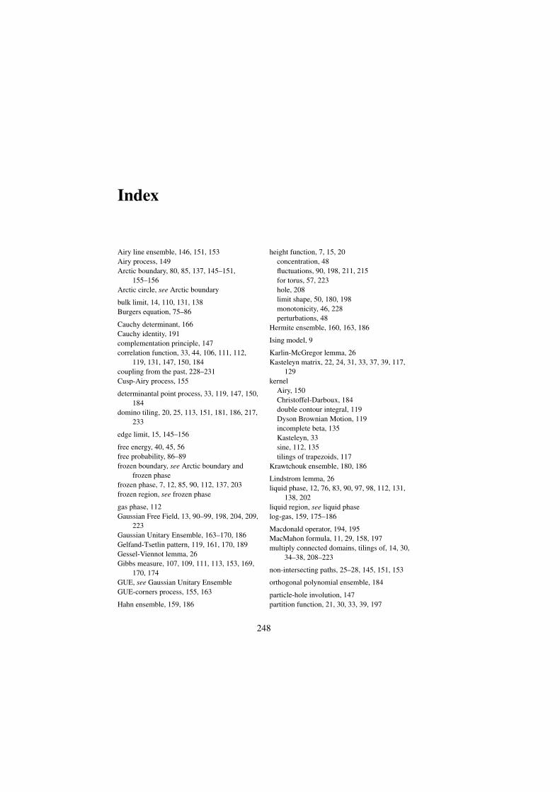
Index
Airy line ensemble, 146, 151, 153Airy process, 149Arctic boundary, 80, 85, 137, 145–151,
155–156Arctic circle, see Arctic boundary
bulk limit, 14, 110, 131, 138Burgers equation, 75–86
Cauchy determinant, 166Cauchy identity, 191complementation principle, 147correlation function, 33, 44, 106, 111, 112,
119, 131, 147, 150, 184coupling from the past, 228–231Cusp-Airy process, 155
determinantal point process, 33, 119, 147, 150,184
domino tiling, 20, 25, 113, 151, 181, 186, 217,233
edge limit, 15, 145–156
free energy, 40, 45, 56free probability, 86–89frozen boundary, see Arctic boundary and
frozen phasefrozen phase, 7, 12, 85, 90, 112, 137, 203frozen region, see frozen phase
gas phase, 112Gaussian Free Field, 13, 90–99, 198, 204, 209,
223Gaussian Unitary Ensemble, 163–170, 186Gelfand-Tsetlin pattern, 119, 161, 170, 189Gessel-Viennot lemma, 26Gibbs measure, 107, 109, 111, 113, 153, 169,
170, 174GUE, see Gaussian Unitary EnsembleGUE-corners process, 155, 163
Hahn ensemble, 159, 186
height function, 7, 15, 20concentration, 48fluctuations, 90, 198, 211, 215for torus, 57, 223hole, 208limit shape, 50, 180, 198monotonicity, 46, 228perturbations, 48
Hermite ensemble, 160, 163, 186
Ising model, 9
Karlin-McGregor lemma, 26Kasteleyn matrix, 22, 24, 31, 33, 37, 39, 117,
129kernel
Airy, 150Christoffel-Darboux, 184double contour integral, 119Dyson Brownian Motion, 119incomplete beta, 135Kasteleyn, 33sine, 112, 135tilings of trapezoids, 117
Krawtchouk ensemble, 180, 186
Lindstrom lemma, 26liquid phase, 12, 76, 83, 90, 97, 98, 112, 131,
138, 202liquid region, see liquid phaselog-gas, 159, 175–186
Macdonald operator, 194, 195MacMahon formula, 11, 29, 158, 197multiply connected domains, tilings of, 14, 30,
34–38, 208–223
non-intersecting paths, 25–28, 145, 151, 153
orthogonal polynomial ensemble, 184
particle-hole involution, 147partition function, 21, 30, 33, 39, 197
248
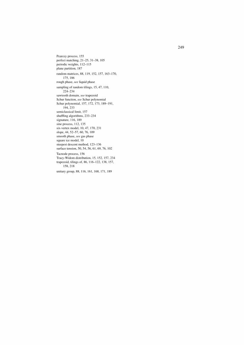
249
Pearcey process, 155perfect matching, 21–25, 31–38, 105periodic weights, 112–115plane partition, 187
random matrices, 88, 119, 152, 157, 163–170,175, 186
rough phase, see liquid phase
sampling of random tilings, 15, 47, 110,224–234
sawtooth domain, see trapezoidSchur function, see Schur polynomialSchur polynomial, 157, 172, 173, 189–191,
194, 233semiclassical limit, 157shuffling algorithms, 233–234signature, 116, 189sine process, 112, 135six-vertex model, 10, 47, 170, 231slope, 44, 52–57, 60, 76, 109smooth phase, see gas phasesquare ice model, 10steepest descent method, 123–136surface tension, 50, 54, 56, 61, 69, 76, 102
Tacnode process, 156Tracy-Widom distribution, 15, 152, 157, 234trapezoid, tilings of, 86, 116–122, 138, 157,
158, 218
unitary group, 88, 116, 161, 168, 171, 189


![Aperiodic tilings [1ex]and substitutions - univ-orleans.fr€¦ · Aperiodic tilings and substitutions Nicolas Ollinger LIFO, Université d’Orléans Journées SDA2, ... Tilings](https://img.pdfslide.us/doc/110x75/5f1071477e708231d4492197/aperiodic-tilings-1exand-substitutions-univ-aperiodic-tilings-and-substitutions.jpg)