Embed Size (px)
Citation preview
Lectures on Dynamical Systems
Anatoly Neishtadt
Lectures for ”Mathematics Access Grid Instruction and Collaboration”(MAGIC) consortium, Loughborough University, 2007
Part 1
LECTURE 1
Introduction
Theory of dynamical systems studies processes which are evolving in time. Thedescription of these processes is given in terms of difference or differentialequations, or iterations of maps.
Example (Fibonacci sequence, 1202)
bk+1 = bk + bk−1, k = 1, 2, . . . ; b0 = 0, b1 = 1
I.Newton (1676): “ 6 aeccdae 13eff 7i 3l 9n 4o 4qrr 4s 9t 12vx” (fundamentalanagram of calculus, in a modern terminology, “It is useful to solve differentialequations”).
H.Poincare is a founder of the modern theory of dynamical systems.
The name of the subject, ”DYNAMICAL SYSTEMS”, came from the title ofclassical book: G.D.Birkhoff, Dynamical Systems. Amer. Math. Soc. Colloq.Publ. 9. American Mathematical Society, New York (1927), 295 pp.
Definition of dynamical system
Definition of dynamical system includes three components:
I phase space (also called state space),
I time,
I law of evolution.
Rather general (but not the most general) definition for these components is asfollows.
I. Phase space is a set whose elements (called “points”) present possible statesof the system at any moment of time. (In our course phase space will usuallybe a smooth finite-dimensional manifold.)II. Time can be either discrete, whose set of values is the set of integernumbers Z, or continuous, whose set of values is the set of real numbers R.III. Law of evolution is the rule which allows us, if we know the state of thesystem at some moment of time, to determine the state of the system at anyother moment of time. (The existence of this law is equivalent to theassumption that our process is deterministic in the past and in the future.)
It is assumed that the law of evolution itself does not depend on time, i.e forany values t, t0 the result of the evolution during the time t starting from themoment of time t0 does not depend on t0.
Definition of dynamical system
Definition of dynamical system includes three components:
I phase space (also called state space),
I time,
I law of evolution.
Rather general (but not the most general) definition for these components is asfollows.
I. Phase space is a set whose elements (called “points”) present possible statesof the system at any moment of time. (In our course phase space will usuallybe a smooth finite-dimensional manifold.)
II. Time can be either discrete, whose set of values is the set of integernumbers Z, or continuous, whose set of values is the set of real numbers R.III. Law of evolution is the rule which allows us, if we know the state of thesystem at some moment of time, to determine the state of the system at anyother moment of time. (The existence of this law is equivalent to theassumption that our process is deterministic in the past and in the future.)
It is assumed that the law of evolution itself does not depend on time, i.e forany values t, t0 the result of the evolution during the time t starting from themoment of time t0 does not depend on t0.
Definition of dynamical system
Definition of dynamical system includes three components:
I phase space (also called state space),
I time,
I law of evolution.
Rather general (but not the most general) definition for these components is asfollows.
I. Phase space is a set whose elements (called “points”) present possible statesof the system at any moment of time. (In our course phase space will usuallybe a smooth finite-dimensional manifold.)II. Time can be either discrete, whose set of values is the set of integernumbers Z, or continuous, whose set of values is the set of real numbers R.
III. Law of evolution is the rule which allows us, if we know the state of thesystem at some moment of time, to determine the state of the system at anyother moment of time. (The existence of this law is equivalent to theassumption that our process is deterministic in the past and in the future.)
It is assumed that the law of evolution itself does not depend on time, i.e forany values t, t0 the result of the evolution during the time t starting from themoment of time t0 does not depend on t0.
Definition of dynamical system
Definition of dynamical system includes three components:
I phase space (also called state space),
I time,
I law of evolution.
Rather general (but not the most general) definition for these components is asfollows.
I. Phase space is a set whose elements (called “points”) present possible statesof the system at any moment of time. (In our course phase space will usuallybe a smooth finite-dimensional manifold.)II. Time can be either discrete, whose set of values is the set of integernumbers Z, or continuous, whose set of values is the set of real numbers R.III. Law of evolution is the rule which allows us, if we know the state of thesystem at some moment of time, to determine the state of the system at anyother moment of time. (The existence of this law is equivalent to theassumption that our process is deterministic in the past and in the future.)
It is assumed that the law of evolution itself does not depend on time, i.e forany values t, t0 the result of the evolution during the time t starting from themoment of time t0 does not depend on t0.
Definition of dynamical system
Definition of dynamical system includes three components:
I phase space (also called state space),
I time,
I law of evolution.
Rather general (but not the most general) definition for these components is asfollows.
I. Phase space is a set whose elements (called “points”) present possible statesof the system at any moment of time. (In our course phase space will usuallybe a smooth finite-dimensional manifold.)II. Time can be either discrete, whose set of values is the set of integernumbers Z, or continuous, whose set of values is the set of real numbers R.III. Law of evolution is the rule which allows us, if we know the state of thesystem at some moment of time, to determine the state of the system at anyother moment of time. (The existence of this law is equivalent to theassumption that our process is deterministic in the past and in the future.)
It is assumed that the law of evolution itself does not depend on time, i.e forany values t, t0 the result of the evolution during the time t starting from themoment of time t0 does not depend on t0.
Definition of dynamical system, continued
Denote X the phase space of our system. Let us introduce the evolutionoperator g t for the time t by means of the following relation: for any statex ∈ X of the system at the moment of time 0 the state of the system at themoment of time t is g tx .So, g t : X → X .
The assumption, that the law of evolution itself does not depend on time and,thus, there exists the evolution operator, implies the following fundamentalidentity:
g s(g tx) = g t+s(x).
Therefore, the set g t is commutative group with respect to the compositionoperation: g sg t = g s(g t).Unity of this group is g 0 which is the identity transformation.The inverse element to g t is g−t .
This group is isomorphic to Z or R for the cases of discrete or continuous timerespectively.
In the case of discrete time, such groups are called one-parametric groups oftransformations with discrete time, or phase cascades.
In the case of continuous time, such groups are just called one-parametricgroups of transformations, or phase flows.
Definition of dynamical system, continued
Now we can give a formal definition.
DefinitionDynamical system is a triple (X , Ξ, G), where X is a set (phase space), Ξ iseither Z or R, and G is a one-parametric group of transformation of X (withdiscrete time if Ξ = Z).
The set g tx , t ∈ Ξ is called a trajectory, or an orbit, of the point x ∈ X .
RemarkFor the case of discrete time gn = (g 1)n. So, the orbit of the point x is. . . , x , g 1x , (g 1)2x , (g 1)3x , . . .
In our course we almost always will have a finite-dimensional smooth manifoldas X and will assume that g tx is smooth with respect to x if Ξ = Z and withrespect to (x , t) if Ξ = R. So, we consider smooth dynamical systems.
Simple examples
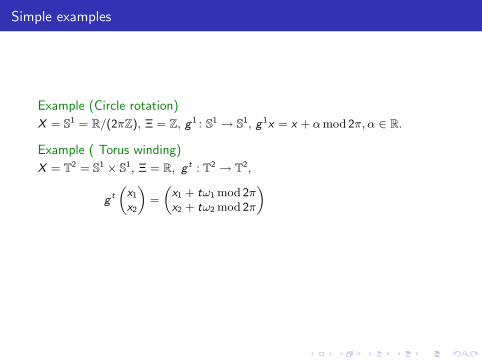
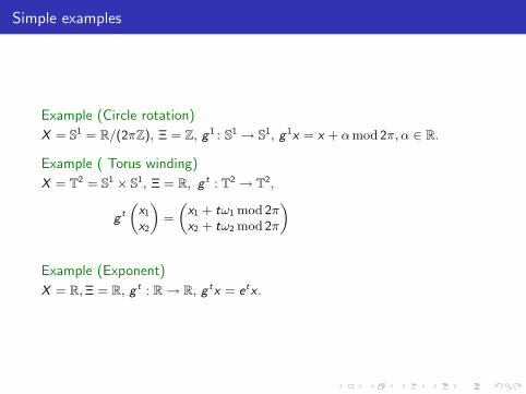
Example (Circle rotation)
X = S1 = R/(2πZ), Ξ = Z, g 1 : S1 → S1, g 1x = x + α mod 2π, α ∈ R.
Example ( Torus winding)
X = T2 = S1 × S1, Ξ = R, g t : T2 → T2,
g t
„x1
x2
«=
„x1 + tω1 mod 2πx2 + tω2 mod 2π
«
Example (Exponent)
X = R, Ξ = R, g t : R → R, g tx = etx .
Simple examples
Example (Circle rotation)
X = S1 = R/(2πZ), Ξ = Z, g 1 : S1 → S1, g 1x = x + α mod 2π, α ∈ R.
Example ( Torus winding)
X = T2 = S1 × S1, Ξ = R, g t : T2 → T2,
g t
„x1
x2
«=
„x1 + tω1 mod 2πx2 + tω2 mod 2π
«
Example (Exponent)
X = R, Ξ = R, g t : R → R, g tx = etx .
Simple examples
Example (Circle rotation)
X = S1 = R/(2πZ), Ξ = Z, g 1 : S1 → S1, g 1x = x + α mod 2π, α ∈ R.
Example ( Torus winding)
X = T2 = S1 × S1, Ξ = R, g t : T2 → T2,
g t
„x1
x2
«=
„x1 + tω1 mod 2πx2 + tω2 mod 2π
«
Example (Exponent)
X = R, Ξ = R, g t : R → R, g tx = etx .
Simple examples
Example (Circle rotation)
X = S1 = R/(2πZ), Ξ = Z, g 1 : S1 → S1, g 1x = x + α mod 2π, α ∈ R.
Example ( Torus winding)
X = T2 = S1 × S1, Ξ = R, g t : T2 → T2,
g t
„x1
x2
«=
„x1 + tω1 mod 2πx2 + tω2 mod 2π
«
Example (Exponent)
X = R, Ξ = R, g t : R → R, g tx = etx .

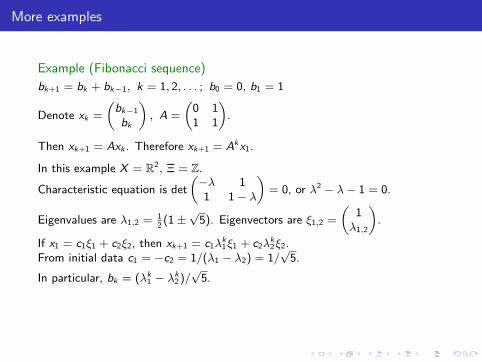
More examples
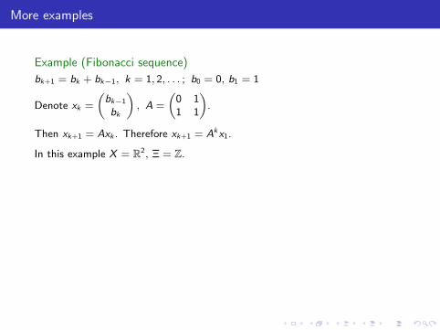
Example (Fibonacci sequence)
bk+1 = bk + bk−1, k = 1, 2, . . . ; b0 = 0, b1 = 1
Denote xk =
„bk−1
bk
«, A =
„0 11 1
«.
Then xk+1 = Axk . Therefore xk+1 = Akx1.
In this example X = R2, Ξ = Z.
Characteristic equation is det
„−λ 11 1− λ
«= 0, or λ2 − λ− 1 = 0.
Eigenvalues are λ1,2 = 12(1±
√5). Eigenvectors are ξ1,2 =
„1
λ1,2
«.
If x1 = c1ξ1 + c2ξ2, then xk+1 = c1λk1ξ1 + c2λ
k2ξ2.
From initial data c1 = −c2 = 1/(λ1 − λ2) = 1/√
5.
In particular, bk = (λk1 − λk
2)/√
5.
Example (Two body problem)
X = R12, Ξ = R
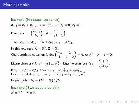
More examples
Example (Fibonacci sequence)
bk+1 = bk + bk−1, k = 1, 2, . . . ; b0 = 0, b1 = 1
Denote xk =
„bk−1
bk
«, A =
„0 11 1
«.
Then xk+1 = Axk . Therefore xk+1 = Akx1.
In this example X = R2, Ξ = Z.
Characteristic equation is det
„−λ 11 1− λ
«= 0, or λ2 − λ− 1 = 0.
Eigenvalues are λ1,2 = 12(1±
√5). Eigenvectors are ξ1,2 =
„1
λ1,2
«.
If x1 = c1ξ1 + c2ξ2, then xk+1 = c1λk1ξ1 + c2λ
k2ξ2.
From initial data c1 = −c2 = 1/(λ1 − λ2) = 1/√
5.
In particular, bk = (λk1 − λk
2)/√
5.
Example (Two body problem)
X = R12, Ξ = R
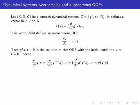
Dynamical systems, vector fields and autonomous ODEs
Let (X , R, G) be a smooth dynamical system, G = g t , t ∈ R. It defines avector field v on X :
v(x) = (d
dtg tx)t=0
This vector field defines an autonomous ODE
dx
dt= v(x)
Then g tx , t ∈ R is the solution to this ODE with the initial condition x att = 0. Indeed,
d
dtg tx = (
d
dεg t+εx)ε=0 = (
d
dεgεg tx)ε=0 = v(g tx)
The other way around, any autonomous ODE whose solutions for all initialconditions are defined for all values of time generates a dynamical system: ashift along trajectories of the ODE is the evolution operator of this dynamicalsystem.
Dynamical systems with continuous time are usually described viacorresponding autonomous ODEs.
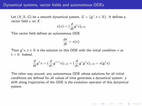
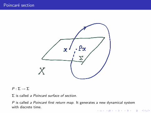
Poincare section
P : Σ → Σ
Σ is called a Poincare surface of section.
P is called a Poincare first return map. It generates a new dynamical systemwith discrete time.
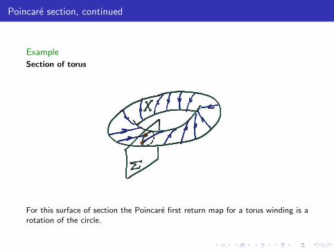
Poincare section, continued
Example
Section of torus
For this surface of section the Poincare first return map for a torus winding is arotation of the circle.
Non-autonomous ODE’s
A non-autonomous ODEdx
dt= v(x , t)
can be reduced to an autonomous one by introducing a new dependent variabley: dy/dt = 1. However, this is often an inappropriate approach because therecurrence properties of the time dependence are thus hidden.
Example (Quasi-periodic time dependence)
dx
dt= v(x , tω), x ∈ Rn, ω ∈ Rm,
function v is 2π-periodic in each of the last m arguments. It is useful to studythe autonomous ODE
dx
dt= v(x , ϕ),
dϕ
dt= ω
whose phase space is Rn × Tm. For m = 1 the Poincare return map for thesection ϕ = 0mod 2π reduces the problem to a dynamical system with discretetime.
Blow-up
For ODEs some solutions may be defined only locally in time, for t− < t < t+,where t−, t+ depend on initial condition. An important example of such abehavior is a “blow-up”, when a solution of a continuous-time system inX = Rn approaches infinity within a finite time.
Example
For equationx = x2, x ∈ R
each solution with a positive (respectively, a negative) initial condition at t = 0tends to +∞ (respectively, −∞) when time approaches some finite moment inthe future (respectively, in the past). The only solution defined for all times isx ≡ 0.
Such equations define only local phase flows.
Some generalisations
1. One can modify the definition of dynamical system taking Ξ = Z+ orΞ = R+ , and G being semigroup of transformations.
2. There are theories in which phase space is an infinite-dimensional functionalspace. (However, even in these theories very often essential events occur in afinite-dimensional submanifold, and so the finite-dimensional case is at the coreof the problem. Moreover, analysis of infinite-dimensional problems oftenfollows the schemes developed for finite-dimensional problems.)
Topics in the course
1. Linear dynamical systems.
2. Normal forms of nonlinear systems.
3. Bifurcations.
4. Perturbations of integrable systems, in particular, KAM-theory.
Exercises
Exercises
1. Consider the sequence1, 2, 4, 8, 1, 3, 6, 1, 2, 5, 1, 2 ,4, 8,. . .
of first digits of consecutive powers of 2. Does a 7 ever appears in thissequence? More generally, does 2n begin with an arbitrary combination ofdigits?
2. Prove that sup0<t<∞
(cos t + sin√
2t) = 2.

LECTURE 2

LINEAR DYNAMICAL SYSTEMS
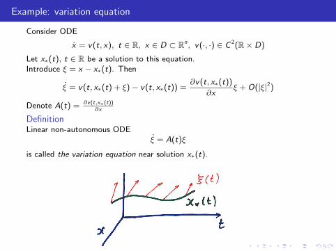
Example: variation equation
Consider ODE
x = v(t, x), t ∈ R, x ∈ D ⊂ Rn, v(·, ·) ∈ C 2(R× D)
Let x∗(t), t ∈ R be a solution to this equation.Introduce ξ = x − x∗(t). Then
ξ = v(t, x∗(t) + ξ)− v(t, x∗(t)) =∂v(t, x∗(t))
∂xξ + O(|ξ|2)
Denote A(t) = ∂v(t,x∗(t))∂x
DefinitionLinear non-autonomous ODE
ξ = A(t)ξ
is called the variation equation near solution x∗(t).
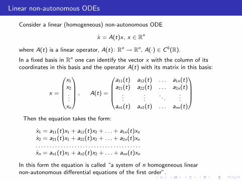
Linear non-autonomous ODEs
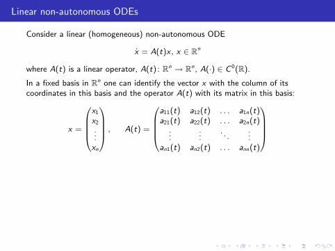
Consider a linear (homogeneous) non-autonomous ODE
x = A(t)x , x ∈ Rn
where A(t) is a linear operator, A(t) : Rn → Rn, A(·) ∈ C 0(R).
In a fixed basis in Rn one can identify the vector x with the column of itscoordinates in this basis and the operator A(t) with its matrix in this basis:
x =
0BBB@x1
x2
...xn
1CCCA , A(t) =
0BBB@a11(t) a12(t) . . . a1n(t)a21(t) a22(t) . . . a2n(t)
......
. . ....
an1(t) an2(t) . . . ann(t)
1CCCAThen the equation takes the form:
x1 = a11(t)x1 + a12(t)x2 + . . . + a1n(t)xn
x2 = a21(t)x1 + a22(t)x2 + . . . + a2n(t)xn
. . . . . . . . . . . . . . . . . . . . . . . . . . . . . . . . . . . . . .xn = an1(t)x1 + an2(t)x2 + . . . + ann(t)xn
In this form the equation is called “a system of n homogeneous linearnon-autonomous differential equations of the first order”.
Linear non-autonomous ODEs
Consider a linear (homogeneous) non-autonomous ODE
x = A(t)x , x ∈ Rn
where A(t) is a linear operator, A(t) : Rn → Rn, A(·) ∈ C 0(R).
In a fixed basis in Rn one can identify the vector x with the column of itscoordinates in this basis and the operator A(t) with its matrix in this basis:
x =
0BBB@x1
x2
...xn
1CCCA , A(t) =
0BBB@a11(t) a12(t) . . . a1n(t)a21(t) a22(t) . . . a2n(t)
......
. . ....
an1(t) an2(t) . . . ann(t)
1CCCA
Then the equation takes the form:
x1 = a11(t)x1 + a12(t)x2 + . . . + a1n(t)xn
x2 = a21(t)x1 + a22(t)x2 + . . . + a2n(t)xn
. . . . . . . . . . . . . . . . . . . . . . . . . . . . . . . . . . . . . .xn = an1(t)x1 + an2(t)x2 + . . . + ann(t)xn
In this form the equation is called “a system of n homogeneous linearnon-autonomous differential equations of the first order”.
Linear non-autonomous ODEs
Consider a linear (homogeneous) non-autonomous ODE
x = A(t)x , x ∈ Rn
where A(t) is a linear operator, A(t) : Rn → Rn, A(·) ∈ C 0(R).
In a fixed basis in Rn one can identify the vector x with the column of itscoordinates in this basis and the operator A(t) with its matrix in this basis:
x =
0BBB@x1
x2
...xn
1CCCA , A(t) =
0BBB@a11(t) a12(t) . . . a1n(t)a21(t) a22(t) . . . a2n(t)
......
. . ....
an1(t) an2(t) . . . ann(t)
1CCCAThen the equation takes the form:
x1 = a11(t)x1 + a12(t)x2 + . . . + a1n(t)xn
x2 = a21(t)x1 + a22(t)x2 + . . . + a2n(t)xn
. . . . . . . . . . . . . . . . . . . . . . . . . . . . . . . . . . . . . .xn = an1(t)x1 + an2(t)x2 + . . . + ann(t)xn
In this form the equation is called “a system of n homogeneous linearnon-autonomous differential equations of the first order”.
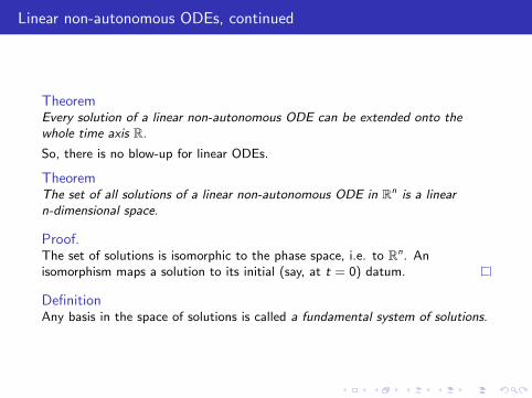
Linear non-autonomous ODEs, continued
TheoremEvery solution of a linear non-autonomous ODE can be extended onto thewhole time axis R.
So, there is no blow-up for linear ODEs.
TheoremThe set of all solutions of a linear non-autonomous ODE in Rn is a linearn-dimensional space.
Proof.The set of solutions is isomorphic to the phase space, i.e. to Rn. Anisomorphism maps a solution to its initial (say, at t = 0) datum.
DefinitionAny basis in the space of solutions is called a fundamental system of solutions.
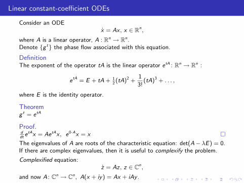
Linear constant-coefficient ODEs
Consider an ODEx = Ax , x ∈ Rn,
where A is a linear operator, A : Rn → Rn.Denote g t the phase flow associated with this equation.
DefinitionThe exponent of the operator tA is the linear operator etA : Rn → Rn :
etA = E + tA + 12(tA)2 +
1
3!(tA)3 + . . . ,
where E is the identity operator.
Theoremg t = etA
Proof.ddt
etAx = AetAx , e0·Ax = x
The eigenvalues of A are roots of the characteristic equation: det(A− λE) = 0.If there are complex eigenvalues, then it is useful to complexify the problem.
Complexified equation:z = Az , z ∈ Cn,
and now A : Cn → Cn, A(x + iy) = Ax + iAy .
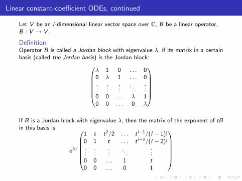
Linear constant-coefficient ODEs, continued
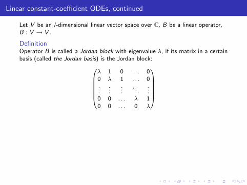
Let V be an l-dimensional linear vector space over C, B be a linear operator,B : V → V .
DefinitionOperator B is called a Jordan block with eigenvalue λ, if its matrix in a certainbasis (called the Jordan basis) is the Jordan block:0BBBBB@
λ 1 0 . . . 00 λ 1 . . . 0...
......
. . ....
0 0 . . . λ 10 0 . . . 0 λ
1CCCCCA
If B is a Jordan block with eigenvalue λ, then the matrix of the exponent of tBin this basis is
eλt
0BBBBB@1 t t2/2 . . . t l−1/(l − 1)!0 1 t . . . t l−2/(l − 2)!...
......
. . ....
0 0 . . . 1 t0 0 . . . 0 1
1CCCCCA
Linear constant-coefficient ODEs, continued
Let V be an l-dimensional linear vector space over C, B be a linear operator,B : V → V .
DefinitionOperator B is called a Jordan block with eigenvalue λ, if its matrix in a certainbasis (called the Jordan basis) is the Jordan block:0BBBBB@
λ 1 0 . . . 00 λ 1 . . . 0...
......
. . ....
0 0 . . . λ 10 0 . . . 0 λ
1CCCCCAIf B is a Jordan block with eigenvalue λ, then the matrix of the exponent of tBin this basis is
eλt
0BBBBB@1 t t2/2 . . . t l−1/(l − 1)!0 1 t . . . t l−2/(l − 2)!...
......
. . ....
0 0 . . . 1 t0 0 . . . 0 1
1CCCCCA
Linear constant-coefficient ODEs, continued
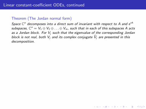
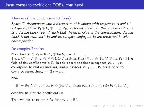
Theorem (The Jordan normal form)
Space Cn decomposes into a direct sum of invariant with respect to A and etA
subspaces, Cn = V1 ⊕V2 ⊕ . . .⊕Vm, such that in each of this subspaces A actsas a Jordan block. For Vj such that the eigenvalue of the corresponding Jordanblock is not real, both Vj and its complex conjugate Vj are presented in thisdecomposition.
De-complexification
Note that Vj ⊕ Vj = ReVj ⊕ ImVj over C.Thus, Cn = V1 ⊕ . . .⊕Vr ⊕ (Re Vr+1 ⊕ ImVr+1)⊕ . . .⊕ (ReVk ⊕ ImVk) if thefield of the coefficients is C. In this decompositions subspaces V1, . . . , Vr
correspond to real eigenvalues, and subspaces Vr+1, . . . , Vk correspond tocomplex eigenvalues, r + 2k = m.
Now
Rn = ReV1 ⊕ . . .⊕ ReVr ⊕ (Re Vr+1 ⊕ ImVr+1)⊕ . . .⊕ (ReVk ⊕ ImVk)
over the field of the coefficients R.
Thus we can calculate etAx for any x ∈ Rn.
Linear constant-coefficient ODEs, continued
Theorem (The Jordan normal form)
Space Cn decomposes into a direct sum of invariant with respect to A and etA
subspaces, Cn = V1 ⊕V2 ⊕ . . .⊕Vm, such that in each of this subspaces A actsas a Jordan block. For Vj such that the eigenvalue of the corresponding Jordanblock is not real, both Vj and its complex conjugate Vj are presented in thisdecomposition.
De-complexification
Note that Vj ⊕ Vj = Re Vj ⊕ ImVj over C.Thus, Cn = V1 ⊕ . . .⊕Vr ⊕ (Re Vr+1 ⊕ ImVr+1)⊕ . . .⊕ (Re Vk ⊕ ImVk) if thefield of the coefficients is C. In this decompositions subspaces V1, . . . , Vr
correspond to real eigenvalues, and subspaces Vr+1, . . . , Vk correspond tocomplex eigenvalues, r + 2k = m.
Now
Rn = ReV1 ⊕ . . .⊕ ReVr ⊕ (Re Vr+1 ⊕ ImVr+1)⊕ . . .⊕ (Re Vk ⊕ ImVk)
over the field of the coefficients R.
Thus we can calculate etAx for any x ∈ Rn.
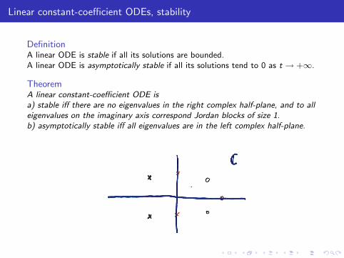
Linear constant-coefficient ODEs, stability
DefinitionA linear ODE is stable if all its solutions are bounded.A linear ODE is asymptotically stable if all its solutions tend to 0 as t → +∞.
TheoremA linear constant-coefficient ODE isa) stable iff there are no eigenvalues in the right complex half-plane, and to alleigenvalues on the imaginary axis correspond Jordan blocks of size 1.b) asymptotically stable iff all eigenvalues are in the left complex half-plane.
Exercises
Exercises
1. Draw all possible phase portraits of linear ODEs in R2.
2. Prove that det(eA) = etr A.
3. May linear operators A and B not commute (i.e. AB 6= BA) if
eA = eB = eA+B = E ?
4. Prove that there is no “blow-up” for a linear non-autonomous ODE.
LECTURE 3
LINEAR DYNAMICAL SYSTEMS
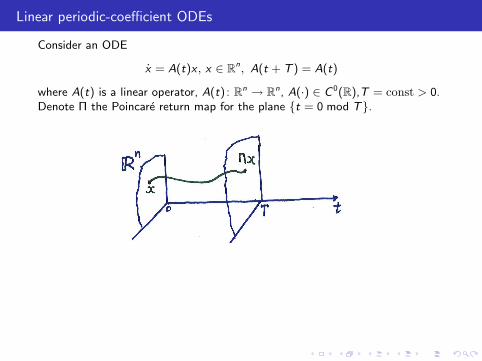
Linear periodic-coefficient ODEs
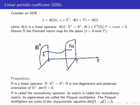
Consider an ODE
x = A(t)x , x ∈ Rn, A(t + T ) = A(t)
where A(t) is a linear operator, A(t) : Rn → Rn, A(·) ∈ C 0(R),T = const > 0.Denote Π the Poincare return map for the plane t = 0 mod T.
Proposition.
Π is a linear operator, Π: Rn → Rn, Π is non-degenerate and preservesorientation of Rn: det Π > 0.
Π is called the monodromy operator, its matrix is called the monodromymatrix, its eigenvalues are called the Floquet multilpliers. The Floquetmultilpliers are roots of the characteristic equation det(Π− ρE) = 0.
Linear periodic-coefficient ODEs
Consider an ODE
x = A(t)x , x ∈ Rn, A(t + T ) = A(t)
where A(t) is a linear operator, A(t) : Rn → Rn, A(·) ∈ C 0(R),T = const > 0.Denote Π the Poincare return map for the plane t = 0 mod T.
Proposition.
Π is a linear operator, Π: Rn → Rn, Π is non-degenerate and preservesorientation of Rn: det Π > 0.
Π is called the monodromy operator, its matrix is called the monodromymatrix, its eigenvalues are called the Floquet multilpliers. The Floquetmultilpliers are roots of the characteristic equation det(Π− ρE) = 0.
Linear periodic-coefficient ODEs, a logarithm
One can complexify both A(t) and Π:A(t) : Cn → Cn, A(t)(x + iy) = A(t)x + iA(t)y ,Π: Cn → Cn, Π(x + iy) = Πx + iΠy .
Let B be a linear operator, B : Cn → Cn.
DefinitionA linear operator K : Cn → Cn is called a logarithm of B if B = eK .
Theorem (Existence of a logarithm)
Any non-degenerate operator has a logarithm.
RemarkLogarithm is not unique; logarithm of a real operator may be complex (example:e iπ+2πk = −1, k ∈ Z). Logarithm is a multi-valued function. Notation: Ln .
Corollary
Take Λ = 1T
Ln Π. Then Π coincides with the evolution operator for the time Tof the constant-coefficient linear ODE z = Λz.
Eigenvalues of K are called Floquet exponents. The relation between Floquetmultipliers ρj and Floquet exponents λj is ρj = eTλj . Real parts of Floquetexponents are Lyapunov exponents.
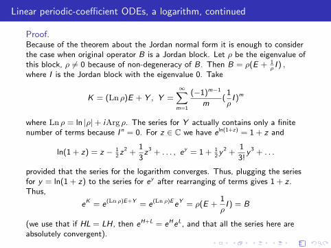
Linear periodic-coefficient ODEs, a logarithm, continued
Proof.Because of the theorem about the Jordan normal form it is enough to considerthe case when original operator B is a Jordan block. Let ρ be the eigenvalue ofthis block, ρ 6= 0 because of non-degeneracy of B. Then B = ρ(E + 1
ρI ) ,
where I is the Jordan block with the eigenvalue 0. Take
K = (Ln ρ)E + Y , Y =∞X
m=1
(−1)m−1
m(1
ρI )m
where Ln ρ = ln |ρ|+ iArg ρ. The series for Y actually contains only a finitenumber of terms because I n = 0. For z ∈ C we have e ln(1+z) = 1 + z and
ln(1 + z) = z − 12z2 +
1
3z3 + . . . , ey = 1 + 1
2y 2 +
1
3!y 3 + . . .
provided that the series for the logarithm converges. Thus, plugging the seriesfor y = ln(1 + z) to the series for ey after rearranging of terms gives 1 + z .Thus,
eK = e(Ln ρ)E+Y = e(Ln ρ)EeY = ρ(E +1
ρI ) = B
(we use that if HL = LH, then eH+L = eHeL, and that all the series here areabsolutely convergent).
Linear periodic-coefficient ODEs, real logarithm
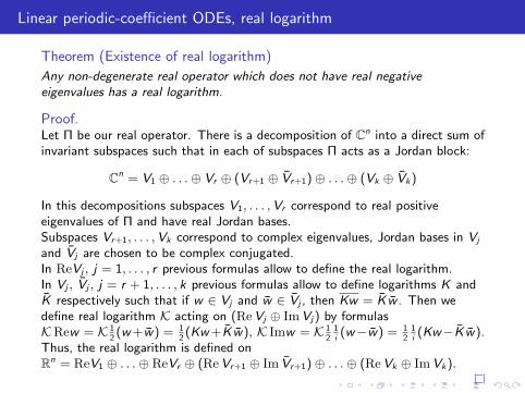
Theorem (Existence of real logarithm)
Any non-degenerate real operator which does not have real negativeeigenvalues has a real logarithm.
Proof.Let Π be our real operator. There is a decomposition of Cn into a direct sum ofinvariant subspaces such that in each of subspaces Π acts as a Jordan block:
Cn = V1 ⊕ . . .⊕ Vr ⊕ (Vr+1 ⊕ Vr+1)⊕ . . .⊕ (Vk ⊕ Vk)
In this decompositions subspaces V1, . . . , Vr correspond to real positiveeigenvalues of Π and have real Jordan bases.Subspaces Vr+1, . . . , Vk correspond to complex eigenvalues, Jordan bases in Vj
and Vj are chosen to be complex conjugated.In ReVj , j = 1, . . . , r previous formulas allow to define the real logarithm.In Vj , Vj , j = r + 1, . . . , k previous formulas allow to define logarithms K andK respectively such that if w ∈ Vj and w ∈ Vj , then Kw = K w . Then wedefine real logarithm K acting on (Re Vj ⊕ ImVj) by formulasKRew = K 1
2(w+w) = 1
2(Kw+K w), K Imw = K 1
21i(w−w) = 1
21i(Kw−K w).
Thus, the real logarithm is defined onRn = ReV1 ⊕ . . .⊕ ReVr ⊕ (Re Vr+1 ⊕ Im Vr+1)⊕ . . .⊕ (ReVk ⊕ ImVk).
Linear periodic-coefficient ODEs, real logarithm
Theorem (Existence of real logarithm)
Any non-degenerate real operator which does not have real negativeeigenvalues has a real logarithm.
Proof.Let Π be our real operator. There is a decomposition of Cn into a direct sum ofinvariant subspaces such that in each of subspaces Π acts as a Jordan block:
Cn = V1 ⊕ . . .⊕ Vr ⊕ (Vr+1 ⊕ Vr+1)⊕ . . .⊕ (Vk ⊕ Vk)
In this decompositions subspaces V1, . . . , Vr correspond to real positiveeigenvalues of Π and have real Jordan bases.Subspaces Vr+1, . . . , Vk correspond to complex eigenvalues, Jordan bases in Vj
and Vj are chosen to be complex conjugated.In ReVj , j = 1, . . . , r previous formulas allow to define the real logarithm.In Vj , Vj , j = r + 1, . . . , k previous formulas allow to define logarithms K andK respectively such that if w ∈ Vj and w ∈ Vj , then Kw = K w . Then wedefine real logarithm K acting on (Re Vj ⊕ ImVj) by formulasKRew = K 1
2(w+w) = 1
2(Kw+K w), K Imw = K 1
21i(w−w) = 1
21i(Kw−K w).
Thus, the real logarithm is defined onRn = ReV1 ⊕ . . .⊕ ReVr ⊕ (Re Vr+1 ⊕ Im Vr+1)⊕ . . .⊕ (Re Vk ⊕ ImVk).
Linear periodic-coefficient ODEs, real logarithm, continued
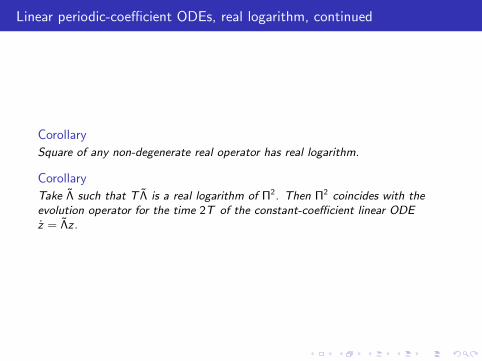
Corollary
Square of any non-degenerate real operator has real logarithm.
Corollary
Take Λ such that T Λ is a real logarithm of Π2. Then Π2 coincides with theevolution operator for the time 2T of the constant-coefficient linear ODEz = Λz.
Linear periodic-coefficient ODEs, Floquet-Lyapunov theory
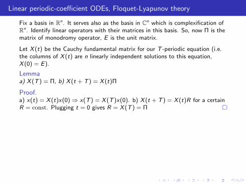
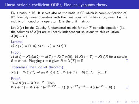
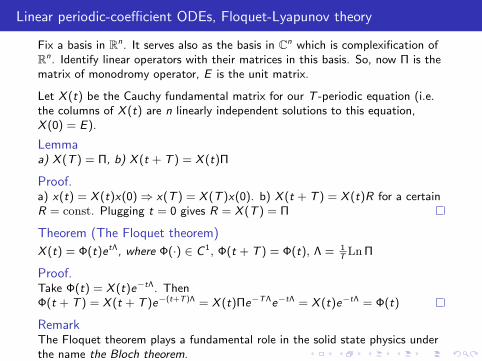
Fix a basis in Rn. It serves also as the basis in Cn which is complexification ofRn. Identify linear operators with their matrices in this basis. So, now Π is thematrix of monodromy operator, E is the unit matrix.
Let X (t) be the Cauchy fundamental matrix for our T -periodic equation (i.e.the columns of X (t) are n linearly independent solutions to this equation,X (0) = E).
Lemmaa) X (T ) = Π, b) X (t + T ) = X (t)Π
Proof.a) x(t) = X (t)x(0) ⇒ x(T ) = X (T )x(0). b) X (t + T ) = X (t)R for a certainR = const. Plugging t = 0 gives R = X (T ) = Π
Theorem (The Floquet theorem)
X (t) = Φ(t)etΛ, where Φ(·) ∈ C 1, Φ(t + T ) = Φ(t), Λ = 1T
Ln Π
Proof.Take Φ(t) = X (t)e−tΛ. ThenΦ(t + T ) = X (t + T )e−(t+T )Λ = X (t)Πe−TΛe−tΛ = X (t)e−tΛ = Φ(t)
RemarkThe Floquet theorem plays a fundamental role in the solid state physics underthe name the Bloch theorem.
Linear periodic-coefficient ODEs, Floquet-Lyapunov theory
Fix a basis in Rn. It serves also as the basis in Cn which is complexification ofRn. Identify linear operators with their matrices in this basis. So, now Π is thematrix of monodromy operator, E is the unit matrix.
Let X (t) be the Cauchy fundamental matrix for our T -periodic equation (i.e.the columns of X (t) are n linearly independent solutions to this equation,X (0) = E).
Lemmaa) X (T ) = Π, b) X (t + T ) = X (t)Π
Proof.a) x(t) = X (t)x(0) ⇒ x(T ) = X (T )x(0). b) X (t + T ) = X (t)R for a certainR = const. Plugging t = 0 gives R = X (T ) = Π
Theorem (The Floquet theorem)
X (t) = Φ(t)etΛ, where Φ(·) ∈ C 1, Φ(t + T ) = Φ(t), Λ = 1T
Ln Π
Proof.Take Φ(t) = X (t)e−tΛ. ThenΦ(t + T ) = X (t + T )e−(t+T )Λ = X (t)Πe−TΛe−tΛ = X (t)e−tΛ = Φ(t)
RemarkThe Floquet theorem plays a fundamental role in the solid state physics underthe name the Bloch theorem.
Linear periodic-coefficient ODEs, Floquet-Lyapunov theory, continued
Theorem (The Lyapunov theorem)
Any linear T-periodic ODE is reducible to a linear constant-coefficient ODE bymeans of a smooth linear T-periodic transformation of variables.
Proof.Let matrices Φ(t) and Λ be as in the Floquet theorem. The requiredtransformation of variables x 7→ y is given by the formula x = Φ(t)y . Theequation in the new variables has the form y = Λy .
RemarkAny linear real T -periodic ODE is reducible to a linear real constant-coefficientODE by means of a smooth linear real 2T -periodic transformation of variables(because Π2 has a real logarithm).
RemarkIf a T -periodic ODE depends smoothly on a parameter, then the transformationof variables in the Lyapunov theorem can also be chosen to be smooth in thisparameter. (Note that this assertion does not follow from the presented proofof the Lyapunov theorem. This property is needed for analysis of bifurcations.)
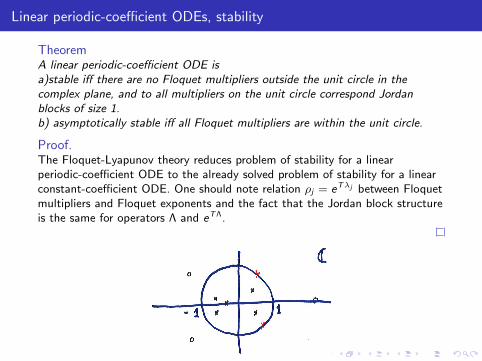
Linear periodic-coefficient ODEs, stability
TheoremA linear periodic-coefficient ODE isa)stable iff there are no Floquet multipliers outside the unit circle in thecomplex plane, and to all multipliers on the unit circle correspond Jordanblocks of size 1.b) asymptotically stable iff all Floquet multipliers are within the unit circle.
Proof.The Floquet-Lyapunov theory reduces problem of stability for a linearperiodic-coefficient ODE to the already solved problem of stability for a linearconstant-coefficient ODE. One should note relation ρj = eTλj between Floquetmultipliers and Floquet exponents and the fact that the Jordan block structureis the same for operators Λ and eTΛ.
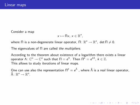
Linear maps
Consider a mapx 7→ Πx , x ∈ Rn,
where Π is a non-degenerate linear operator, Π: Rn → Rn, detΠ 6= 0.
The eigenvalues of Π are called the multipliers.
According to the theorem about existence of a logarithm there exists a linearoperator Λ: Cn → Cn such that Π = eΛ. Then Πk = ekΛ, k ∈ Z.This allows to study iterations of linear maps.
One can use also the representation Π2 = e Λ , where Λ is a real linear operator,Λ : Rn → Rn.
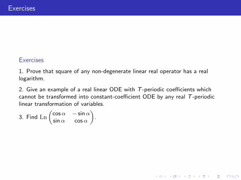
Exercises
Exercises
1. Prove that square of any non-degenerate linear real operator has a reallogarithm.
2. Give an example of a real linear ODE with T -periodic coefficients whichcannot be transformed into constant-coefficient ODE by any real T -periodiclinear transformation of variables.
3. Find Ln
„cos α − sin αsin α cos α
«.
Bibliography
Arnold, V.I. Ordinary differential equations. Springer-Verlag, Berlin, 2006.
Arnold, V. I. Geometrical methods in the theory of ordinary differentialequations. Springer-Verlag, New York, 1988.
Arnold, V. I. Mathematical methods of classical mechanics. Springer-Verlag,New York, 1989. p
Coddington, E. A.; Levinson, N. Theory of ordinary differential equations.McGraw-Hill Book Company, Inc., New York-Toronto-London, 1955.
Dynamical systems. I, Encyclopaedia Math. Sci., 1, Springer-Verlag, Berlin,1998
Hartman, P. Ordinary differential equations. (SIAM), Philadelphia, PA, 2002.
Shilnikov, L. P.; Shilnikov, A. L.; Turaev, D. V.; Chua, L. O. Methods ofqualitative theory in nonlinear dynamics. Part I. World Scientific, Inc., RiverEdge, NJ, 1998.
Yakubovich, V. A.; Starzhinskii, V. M. Linear differential equations withperiodic coefficients. 1, 2. Halsted Press [John Wiley and Sons] NewYork-Toronto, 1975

LECTURE 4

LINEAR DYNAMICAL SYSTEMS
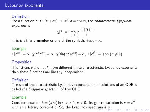
Lyapunov exponents
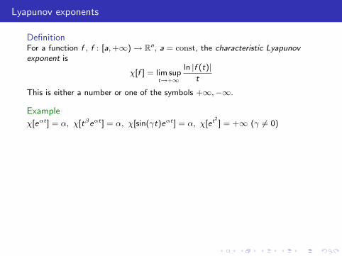
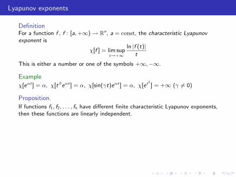
DefinitionFor a function f , f : [a, +∞) → Rn, a = const, the characteristic Lyapunovexponent is
χ[f ] = lim supt→+∞
ln |f (t)|t
This is either a number or one of the symbols +∞,−∞.
Example
χ[eαt ] = α, χ[tβeαt ] = α, χ[sin(γt)eαt ] = α, χ[et2 ] = +∞ (γ 6= 0)
Proposition.
If functions f1, f2, . . . , fn have different finite characteristic Lyapunov exponents,then these functions are linearly independent.
DefinitionThe set of the characteristic Lyapunov exponents of all solutions of an ODE iscalled the Lyapunov spectrum of this ODE
Example
Consider equation x = (x/t) ln x , t > 0, x > 0. Its general solution is x = ect
with an arbitrary constant c. So, the Lyapunov spectrum is R.
Lyapunov exponents
DefinitionFor a function f , f : [a, +∞) → Rn, a = const, the characteristic Lyapunovexponent is
χ[f ] = lim supt→+∞
ln |f (t)|t
This is either a number or one of the symbols +∞,−∞.
Example
χ[eαt ] = α, χ[tβeαt ] = α, χ[sin(γt)eαt ] = α, χ[et2 ] = +∞ (γ 6= 0)
Proposition.
If functions f1, f2, . . . , fn have different finite characteristic Lyapunov exponents,then these functions are linearly independent.
DefinitionThe set of the characteristic Lyapunov exponents of all solutions of an ODE iscalled the Lyapunov spectrum of this ODE
Example
Consider equation x = (x/t) ln x , t > 0, x > 0. Its general solution is x = ect
with an arbitrary constant c. So, the Lyapunov spectrum is R.
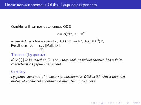
Linear non-autonomous ODEs, Lyapunov exponents
Consider a linear non-autonomous ODE
x = A(t)x , x ∈ Rn
where A(t) is a linear operator, A(t) : Rn → Rn, A(·) ∈ C 0(R).Recall that ‖A‖ = sup
x 6=0‖Ax‖/‖x‖.
Theorem (Lyapunov)
If ‖A(·)‖ is bounded on [0, +∞), then each nontrivial solution has a finitecharacteristic Lyapunov exponent.
Corollary
Lyapunov spectrum of a linear non-autonomous ODE in Rn with a boundedmatrix of coefficients contains no more than n elements.
Exercises
Exercises
1. Prove that the equation
x =
„0 1
2/t2 0
«x
can not be transformed into a constant-coefficient linear equation by means oftransformation of variables of the form y = L(t)x , whereL(·) ∈ C 1(R), |L| < const, |L| < const, |L−1| < const.
2. Let X (t) be a fundamental matrix for the equation x = A(t)x . Prove theLiouville - Ostrogradski formula:
det(X (t)) = det(X (0))eR t0 tr A(τ)dτ
.
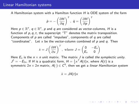
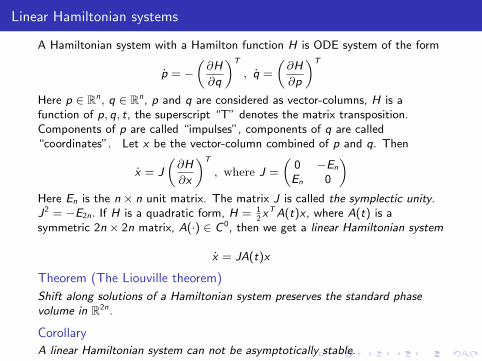
Linear Hamiltonian systems
A Hamiltonian system with a Hamilton function H is ODE system of the form
p = −„
∂H
∂q
«T
, q =
„∂H
∂p
«T
Here p ∈ Rn, q ∈ Rn, p and q are considered as vector-columns, H is afunction of p, q, t, the superscript “T” denotes the matrix transposition.Components of p are called “impulses”, components of q are called“coordinates”.
Let x be the vector-column combined of p and q. Then
x = J
„∂H
∂x
«T
, where J =
„0 −En
En 0
«Here En is the n × n unit matrix. The matrix J is called the symplectic unity.J2 = −E2n. If H is a quadratic form, H = 1
2xTA(t)x , where A(t) is a
symmetric 2n × 2n matrix, A(·) ∈ C 0, then we get a linear Hamiltonian system
x = JA(t)x
Theorem (The Liouville theorem)
Shift along solutions of a Hamiltonian system preserves the standard phasevolume in R2n.
Corollary
A linear Hamiltonian system can not be asymptotically stable.
Linear Hamiltonian systems
A Hamiltonian system with a Hamilton function H is ODE system of the form
p = −„
∂H
∂q
«T
, q =
„∂H
∂p
«T
Here p ∈ Rn, q ∈ Rn, p and q are considered as vector-columns, H is afunction of p, q, t, the superscript “T” denotes the matrix transposition.Components of p are called “impulses”, components of q are called“coordinates”. Let x be the vector-column combined of p and q. Then
x = J
„∂H
∂x
«T
, where J =
„0 −En
En 0
«Here En is the n × n unit matrix. The matrix J is called the symplectic unity.J2 = −E2n. If H is a quadratic form, H = 1
2xTA(t)x , where A(t) is a
symmetric 2n × 2n matrix, A(·) ∈ C 0, then we get a linear Hamiltonian system
x = JA(t)x
Theorem (The Liouville theorem)
Shift along solutions of a Hamiltonian system preserves the standard phasevolume in R2n.
Corollary
A linear Hamiltonian system can not be asymptotically stable.
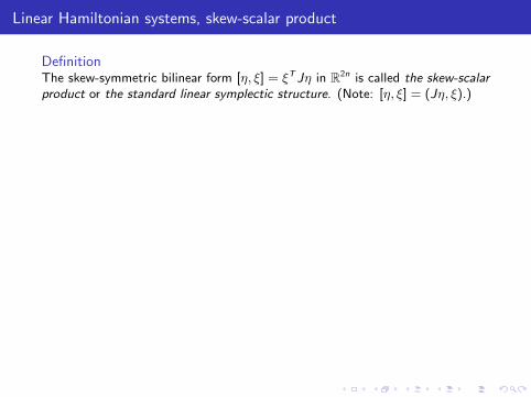
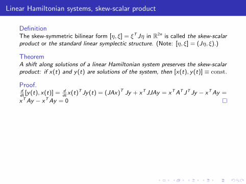
Linear Hamiltonian systems, skew-scalar product
DefinitionThe skew-symmetric bilinear form [η, ξ] = ξTJη in R2n is called the skew-scalarproduct or the standard linear symplectic structure. (Note: [η, ξ] = (Jη, ξ).)
TheoremA shift along solutions of a linear Hamiltonian system preserves the skew-scalarproduct: if x(t) and y(t) are solutions of the system, then [x(t), y(t)] ≡ const.
Proof.ddt
[y(t), x(t)] = ddt
x(t)TJy(t) = (JAx)T Jy + xTJJAy = xTATJTJy − xTAy =
xTAy − xTAy = 0
Corollary
Let X (t) be the Cauchy fundamental matrix for our Hamiltonian system (i.e.the columns of X (t) are n linearly independent solutions to this system,X (0) = E2n). Then XT (t)JX (t) = J for all t ∈ R.
Proof.Elements of matrix XT (t)JX (t) are skew-scalar products of solutions, and sothis is a constant matrix.From the condition at t = 0 we get XT (t)JX (t) = J.
Linear symplectic transformations
DefinitionA 2n × 2n matrix M which satisfies the relation MTJM = J is called asymplectic matrix. A linear transformation of variables with a symplectic matrixis called a linear symplectic transformation of variables.
Corollary
The Cauchy fundamental matrix for linear Hamiltonian system at any momentof time is a symplectic matrix. A shift along solutions of a linear Hamiltoniansystem is a linear symplectic transformation.
TheoremA linear transformations of variables is a symplectic transformations if and onlyif it preserves the skew-scalar product: [Mη, Mξ] = [η, ξ] for anyξ ∈ R2n, η ∈ R2n; here M is the matrix of the transformation.
Proof.[Mη, Mξ] = ξTMTJMη
TheoremSymplectic matrices form a group.
The group of symplectic 2n × 2n matrices is called the symplectic group ofdegree 2n and is denoted as Sp(2n). (The same name is used for the group oflinear symplectic transformations of R2n.)
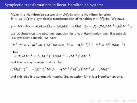
Symplectic transformations in linear Hamiltonian systems
Make in a Hamiltonian system x = JA(t)x with a Hamilton functionH = 1
2xTA(t)x a symplectic transformation of variables y = M(t)x . We have
y = Mx+Mx = MJAx+Mx = (MJAM−1+MM−1)y = J(−JMJAM−1−JMM−1)y
Let us show that the obtained equation for y is a Hamiltonian one. Because Mis a symplectic matrix, we have
MTJM = J, MTJM + MTJM = 0, M = −J(M−1)TJ, MT = MTJMM−1J
Thus−JMJAM−1 = JJ(M−1)TJJAM−1 = (M−1)TAM−1,
and this is a symmetric matrix. And
(JMM−1)T = −(M−1)T MTJ = −(M−1)TMTJMM−1JJ = JMM−1
and this also is a symmetric matrix. So, equation for y is a Hamiltonian one.
Note, that if M = const, then the Hamilton function for the new system
H = 12yT (M−1)TA(t)M−1y
is just the old Hamilton function expressed through the new variables.
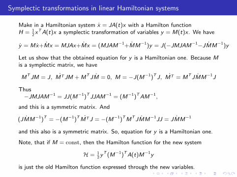
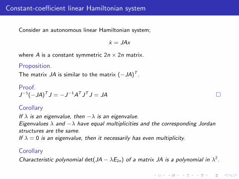
Constant-coefficient linear Hamiltonian system
Consider an autonomous linear Hamiltonian system;
x = JAx
where A is a constant symmetric 2n × 2n matrix.
Proposition.
The matrix JA is similar to the matrix (−JA)T .
Proof.J−1(−JA)TJ = −J−1ATJTJ = JA
Corollary
If λ is an eigenvalue, then −λ is an eigenvalue.Eigenvalues λ and −λ have equal multiplicities and the corresponding Jordanstructures are the same.If λ = 0 is an eigenvalue, then it necessarily has even multiplicity.
Corollary
Characteristic polynomial det(JA− λE2n) of a matrix JA is a polynomial in λ2.
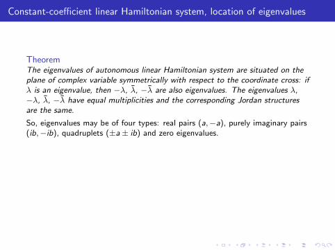
Constant-coefficient linear Hamiltonian system, location of eigenvalues
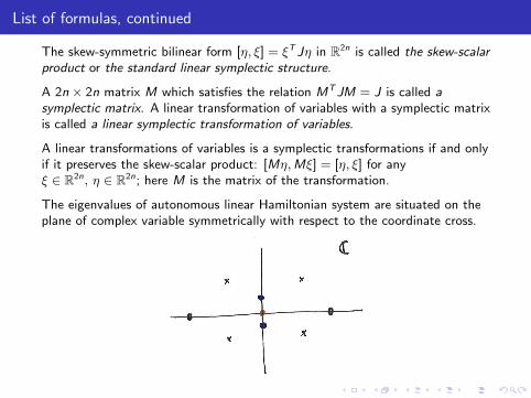
TheoremThe eigenvalues of autonomous linear Hamiltonian system are situated on theplane of complex variable symmetrically with respect to the coordinate cross: ifλ is an eigenvalue, then −λ, λ, −λ are also eigenvalues. The eigenvalues λ,−λ, λ, −λ have equal multiplicities and the corresponding Jordan structuresare the same.
So, eigenvalues may be of four types: real pairs (a,−a), purely imaginary pairs(ib,−ib), quadruplets (±a± ib) and zero eigenvalues.
Corollary
If there is a purely imaginary simple eigenvalue, then it remains on theimaginary axis under a small perturbation of the Hamiltonian. Similarly, a realsimple eigenvalue remains real under a small perturbation of the Hamiltonian.
So, the system may loss stability under a small perturbation of the Hamiltonianonly if there is 1 : 1 resonance.
Constant-coefficient linear Hamiltonian system, location of eigenvalues
TheoremThe eigenvalues of autonomous linear Hamiltonian system are situated on theplane of complex variable symmetrically with respect to the coordinate cross: ifλ is an eigenvalue, then −λ, λ, −λ are also eigenvalues. The eigenvalues λ,−λ, λ, −λ have equal multiplicities and the corresponding Jordan structuresare the same.
So, eigenvalues may be of four types: real pairs (a,−a), purely imaginary pairs(ib,−ib), quadruplets (±a± ib) and zero eigenvalues.
Corollary
If there is a purely imaginary simple eigenvalue, then it remains on theimaginary axis under a small perturbation of the Hamiltonian. Similarly, a realsimple eigenvalue remains real under a small perturbation of the Hamiltonian.
So, the system may loss stability under a small perturbation of the Hamiltonianonly if there is 1 : 1 resonance.

Bibliography
Arnold, V.I. Ordinary differential equations. Springer-Verlag, Berlin, 2006.
Arnold, V. I. Geometrical methods in the theory of ordinary differentialequations. Springer-Verlag, New York, 1988.
Arnold, V. I. Mathematical methods of classical mechanics. Springer-Verlag,New York, 1989. p
Coddington, E. A.; Levinson, N. Theory of ordinary differential equations.McGraw-Hill Book Company, Inc., New York-Toronto-London, 1955.
Dynamical systems. I, Encyclopaedia Math. Sci., 1, Springer-Verlag, Berlin,1998
Hartman, P. Ordinary differential equations. (SIAM), Philadelphia, PA, 2002.
Shilnikov, L. P.; Shilnikov, A. L.; Turaev, D. V.; Chua, L. O. Methods ofqualitative theory in nonlinear dynamics. Part I. World Scientific, Inc., RiverEdge, NJ, 1998.
Yakubovich, V. A.; Starzhinskii, V. M. Linear differential equations withperiodic coefficients. 1, 2. Halsted Press [John Wiley and Sons] NewYork-Toronto, 1975
LECTURE 5
LINEAR HAMILTONIAN SYSTEMS
List of formulas
A Hamiltonian system with a Hamilton function H is an ODE system of theform
p = −„
∂H
∂q
«T
, q =
„∂H
∂p
«T
Here p ∈ Rn, q ∈ Rn, p and q are considered as vector-columns, H is a functionof p, q, t, the superscript “T” denotes the matrix transposition. Components ofp are called “impulses”, components of q are called “coordinates”.
Let x be the vector-column combined of p and q. Then
x = J
„∂H
∂x
«T
, where J =
„0 −En
En 0
«The matrix J is called the symplectic unity. J2 = −E2n.
If H is a quadratic form, H = 12xTA(t)x , where A(t) is a symmetric 2n × 2n
matrix, A(·) ∈ C 0, then we get a linear Hamiltonian system
x = JA(t)x
List of formulas, continued
The skew-symmetric bilinear form [η, ξ] = ξTJη in R2n is called the skew-scalarproduct or the standard linear symplectic structure.
A 2n × 2n matrix M which satisfies the relation MTJM = J is called asymplectic matrix. A linear transformation of variables with a symplectic matrixis called a linear symplectic transformation of variables.
A linear transformations of variables is a symplectic transformations if and onlyif it preserves the skew-scalar product: [Mη, Mξ] = [η, ξ] for anyξ ∈ R2n, η ∈ R2n; here M is the matrix of the transformation.
The eigenvalues of autonomous linear Hamiltonian system are situated on theplane of complex variable symmetrically with respect to the coordinate cross.
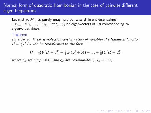
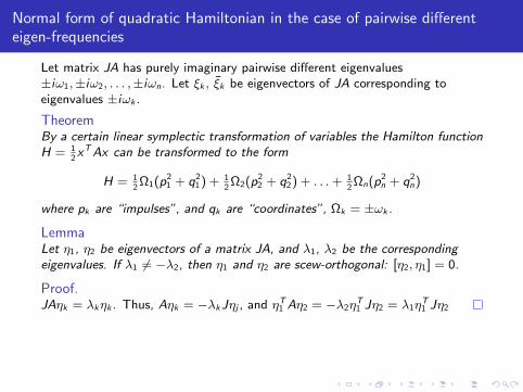
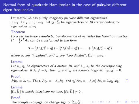
Normal form of quadratic Hamiltonian in the case of pairwise differenteigen-frequencies
Let matrix JA has purely imaginary pairwise different eigenvalues±iω1,±iω2, . . . ,±iωn. Let ξk , ξk be eigenvectors of JA corresponding toeigenvalues ±iωk .
TheoremBy a certain linear symplectic transformation of variables the Hamilton functionH = 1
2xTAx can be transformed to the form
H = 12Ω1(p
21 + q2
1) + 12Ω2(p
22 + q2
2) + . . . + 12Ωn(p
2n + q2
n)
where pk are “impulses”, and qk are “coordinates”, Ωk = ±ωk .
LemmaLet η1, η2 be eigenvectors of a matrix JA, and λ1, λ2 be the correspondingeigenvalues. If λ1 6= −λ2, then η1 and η2 are scew-orthogonal: [η2, η1] = 0.
Proof.JAηk = λkηk . Thus, Aηk = −λkJηj , and ηT
1 Aη2 = −λ2ηT1 Jη2 = λ1η
T1 Jη2
Lemma[ξk , ξk ] is purely imaginary number, [ξk , ξk ] 6= 0 .
Proof.The complex conjugation change sign of [ξk , ξk ].
Without loss of generality we may assume that [ξk , ξk ] is equal either i or −i .
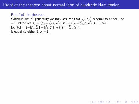
Proof of the theorem about normal form of quadratic Hamiltonian
Proof of the theorem.Without loss of generality we may assume that [ξk , ξk ] is equal to either i or−i . Introduce ak = (ξk + ξk)/
√2, bk = (ξk − ξk)/(
√2i).
Then[ak , bk ] = (−[ξk , ξk ] + [ξk , ξk ])/(2i) = [ξk , ξk ]/iis equal to either 1 or −1. Introduce new vectors uk , vk as follows.If [ak , bk ] = 1, then uk = ak , vk = bk .If [ak , bk ] = −1, then uk = bk , vk = ak .Thus, [uk , vk ] = 1, [uk , vj ] = 0, j 6= k.Choose as the new basis in R2n vectors u1, u2, . . . , un, v1, v2, . . . , vn (in thisorder). The matrix of transformation of vector’s coordinates for this change ofbasis is a symplectic one. In the new coordinates the Hamilton function hasthe required form.
The form of the Hamiltonian shows that the phase space is a direct product ofof invariant two-dimensional mutually skew-orthogonal planes. Dynamics in kthplane is decribed by the Hamilton function Hk = 1
2Ωk(p
2k + q2
k); it is called apartial Hamilton function, or just a partial Hamiltonian. This is the Hamiltonfunction of a linear oscillator with the frequency Ωk . In the plane qk , pk phasecurves are circles. Rotation on this circles is clockwise, if Ωk > 0, andcounterclockwise, if Ωk < 0. Values |Ωk | are called eigen-frequencies of thesystem. Phase space R2n is foliated (with singularities) by n-dimensionalinvariant tori.
Proof of the theorem about normal form of quadratic Hamiltonian
Proof of the theorem.Without loss of generality we may assume that [ξk , ξk ] is equal to either i or−i . Introduce ak = (ξk + ξk)/
√2, bk = (ξk − ξk)/(
√2i). Then
[ak , bk ] = (−[ξk , ξk ] + [ξk , ξk ])/(2i) = [ξk , ξk ]/iis equal to either 1 or −1.
Introduce new vectors uk , vk as follows.If [ak , bk ] = 1, then uk = ak , vk = bk .If [ak , bk ] = −1, then uk = bk , vk = ak .Thus, [uk , vk ] = 1, [uk , vj ] = 0, j 6= k.Choose as the new basis in R2n vectors u1, u2, . . . , un, v1, v2, . . . , vn (in thisorder). The matrix of transformation of vector’s coordinates for this change ofbasis is a symplectic one. In the new coordinates the Hamilton function hasthe required form.
The form of the Hamiltonian shows that the phase space is a direct product ofof invariant two-dimensional mutually skew-orthogonal planes. Dynamics in kthplane is decribed by the Hamilton function Hk = 1
2Ωk(p
2k + q2
k); it is called apartial Hamilton function, or just a partial Hamiltonian. This is the Hamiltonfunction of a linear oscillator with the frequency Ωk . In the plane qk , pk phasecurves are circles. Rotation on this circles is clockwise, if Ωk > 0, andcounterclockwise, if Ωk < 0. Values |Ωk | are called eigen-frequencies of thesystem. Phase space R2n is foliated (with singularities) by n-dimensionalinvariant tori.
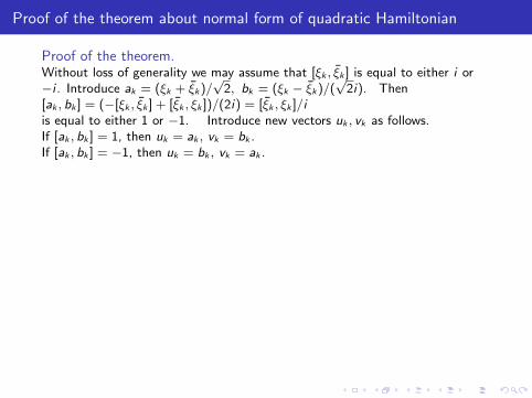
Proof of the theorem about normal form of quadratic Hamiltonian
Proof of the theorem.Without loss of generality we may assume that [ξk , ξk ] is equal to either i or−i . Introduce ak = (ξk + ξk)/
√2, bk = (ξk − ξk)/(
√2i). Then
[ak , bk ] = (−[ξk , ξk ] + [ξk , ξk ])/(2i) = [ξk , ξk ]/iis equal to either 1 or −1. Introduce new vectors uk , vk as follows.If [ak , bk ] = 1, then uk = ak , vk = bk .If [ak , bk ] = −1, then uk = bk , vk = ak .
Thus, [uk , vk ] = 1, [uk , vj ] = 0, j 6= k.Choose as the new basis in R2n vectors u1, u2, . . . , un, v1, v2, . . . , vn (in thisorder). The matrix of transformation of vector’s coordinates for this change ofbasis is a symplectic one. In the new coordinates the Hamilton function hasthe required form.
The form of the Hamiltonian shows that the phase space is a direct product ofof invariant two-dimensional mutually skew-orthogonal planes. Dynamics in kthplane is decribed by the Hamilton function Hk = 1
2Ωk(p
2k + q2
k); it is called apartial Hamilton function, or just a partial Hamiltonian. This is the Hamiltonfunction of a linear oscillator with the frequency Ωk . In the plane qk , pk phasecurves are circles. Rotation on this circles is clockwise, if Ωk > 0, andcounterclockwise, if Ωk < 0. Values |Ωk | are called eigen-frequencies of thesystem. Phase space R2n is foliated (with singularities) by n-dimensionalinvariant tori.
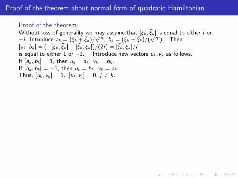
Proof of the theorem about normal form of quadratic Hamiltonian
Proof of the theorem.Without loss of generality we may assume that [ξk , ξk ] is equal to either i or−i . Introduce ak = (ξk + ξk)/
√2, bk = (ξk − ξk)/(
√2i). Then
[ak , bk ] = (−[ξk , ξk ] + [ξk , ξk ])/(2i) = [ξk , ξk ]/iis equal to either 1 or −1. Introduce new vectors uk , vk as follows.If [ak , bk ] = 1, then uk = ak , vk = bk .If [ak , bk ] = −1, then uk = bk , vk = ak .Thus, [uk , vk ] = 1, [uk , vj ] = 0, j 6= k.
Choose as the new basis in R2n vectors u1, u2, . . . , un, v1, v2, . . . , vn (in thisorder). The matrix of transformation of vector’s coordinates for this change ofbasis is a symplectic one. In the new coordinates the Hamilton function hasthe required form.
The form of the Hamiltonian shows that the phase space is a direct product ofof invariant two-dimensional mutually skew-orthogonal planes. Dynamics in kthplane is decribed by the Hamilton function Hk = 1
2Ωk(p
2k + q2
k); it is called apartial Hamilton function, or just a partial Hamiltonian. This is the Hamiltonfunction of a linear oscillator with the frequency Ωk . In the plane qk , pk phasecurves are circles. Rotation on this circles is clockwise, if Ωk > 0, andcounterclockwise, if Ωk < 0. Values |Ωk | are called eigen-frequencies of thesystem. Phase space R2n is foliated (with singularities) by n-dimensionalinvariant tori.
Proof of the theorem about normal form of quadratic Hamiltonian
Proof of the theorem.Without loss of generality we may assume that [ξk , ξk ] is equal to either i or−i . Introduce ak = (ξk + ξk)/
√2, bk = (ξk − ξk)/(
√2i). Then
[ak , bk ] = (−[ξk , ξk ] + [ξk , ξk ])/(2i) = [ξk , ξk ]/iis equal to either 1 or −1. Introduce new vectors uk , vk as follows.If [ak , bk ] = 1, then uk = ak , vk = bk .If [ak , bk ] = −1, then uk = bk , vk = ak .Thus, [uk , vk ] = 1, [uk , vj ] = 0, j 6= k.Choose as the new basis in R2n vectors u1, u2, . . . , un, v1, v2, . . . , vn (in thisorder). The matrix of transformation of vector’s coordinates for this change ofbasis is a symplectic one.
In the new coordinates the Hamilton function hasthe required form.
The form of the Hamiltonian shows that the phase space is a direct product ofof invariant two-dimensional mutually skew-orthogonal planes. Dynamics in kthplane is decribed by the Hamilton function Hk = 1
2Ωk(p
2k + q2
k); it is called apartial Hamilton function, or just a partial Hamiltonian. This is the Hamiltonfunction of a linear oscillator with the frequency Ωk . In the plane qk , pk phasecurves are circles. Rotation on this circles is clockwise, if Ωk > 0, andcounterclockwise, if Ωk < 0. Values |Ωk | are called eigen-frequencies of thesystem. Phase space R2n is foliated (with singularities) by n-dimensionalinvariant tori.
Proof of the theorem about normal form of quadratic Hamiltonian
Proof of the theorem.Without loss of generality we may assume that [ξk , ξk ] is equal to either i or−i . Introduce ak = (ξk + ξk)/
√2, bk = (ξk − ξk)/(
√2i). Then
[ak , bk ] = (−[ξk , ξk ] + [ξk , ξk ])/(2i) = [ξk , ξk ]/iis equal to either 1 or −1. Introduce new vectors uk , vk as follows.If [ak , bk ] = 1, then uk = ak , vk = bk .If [ak , bk ] = −1, then uk = bk , vk = ak .Thus, [uk , vk ] = 1, [uk , vj ] = 0, j 6= k.Choose as the new basis in R2n vectors u1, u2, . . . , un, v1, v2, . . . , vn (in thisorder). The matrix of transformation of vector’s coordinates for this change ofbasis is a symplectic one. In the new coordinates the Hamilton function hasthe required form.
The form of the Hamiltonian shows that the phase space is a direct product ofof invariant two-dimensional mutually skew-orthogonal planes. Dynamics in kthplane is decribed by the Hamilton function Hk = 1
2Ωk(p
2k + q2
k); it is called apartial Hamilton function, or just a partial Hamiltonian. This is the Hamiltonfunction of a linear oscillator with the frequency Ωk . In the plane qk , pk phasecurves are circles. Rotation on this circles is clockwise, if Ωk > 0, andcounterclockwise, if Ωk < 0. Values |Ωk | are called eigen-frequencies of thesystem. Phase space R2n is foliated (with singularities) by n-dimensionalinvariant tori.
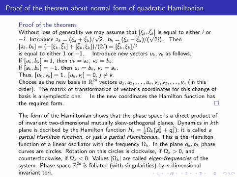
On normal forms of quadratic Hamiltonians
Theorem (Williamson)
There exists a real symplectic linear change of variables reducing theHamiltonian to a sum of partial Hamiltonians (functions of disjoint subsets ofconjugate variables), and the matrix of the system, correspondingly, to ablock-diagonal form. Each partial Hamiltonian corresponds either to a real pair,or to an imaginary pair, or to a quadruplet of eigenvalues, or to a zeroeigenvalue. The partial Hamiltonians are determined, up to a sign, by theJordan blocks of the operator JA.
The list of partial Hamiltonians is contained in the paper by J.Williamson(1936).
On stability loss in constant-coefficient linear Hamiltonian systems
When parameters of a stable constant-coefficient linear Hamiltonian system arechanging, the eigenvalues move on the imaginary axis. When eigenvaluescollide they may leave the imaginary axis. However, collision of not each pair ofeigenvalues is dangerous, some eigenvalues necessarily pass through each otherwithout leaving the imaginary axis.
While all eigenvalues are simple the Hamilton function can be reduced to thenormal form
H = 12Ω1(p
21 + q2
1) + 12Ω2(p
22 + q2
2) + . . . + 12Ωn(p
2n + q2
n)
We say that a partial Hamilton function Hk = 12Ωk(p
2k + q2
k) is positive(negative), if Ωk is positive (respectively, negative).
TheoremIf imaginary eigenvalues corresponding to partial Hamilton functions having thesame sign collide not at the point 0, the system does not loss its stability. Inparticular, when these eigenvalues collide, the matrix of the Hamiltoniansystem does not have Jordan blocks of sizes bigger than 1.
On linear natural Hamiltonian systems
For a natural Hamiltonian system its Hamilton function H is the sum of akinetic energy T = T (p, q) = 1
2pTK−1(q)p and a potential energy V (q) :
H = T + V .Here K(q) is a positive definite matrix.
For a linear natural Hamiltoniansystem K = const and V is a quadratic form: V = 1
2qTDq.
TheoremIn any linear natural Hamiltonian system all non-zero eigenvalues are either realor pure imaginary. To each non-zero eigenvalue correspond only Jordan blocksof size 1. To zero eigenvalue correspond Jordan blocks of size 2.
Corollary
For linear natural Hamiltonian system collision of non-zero eigenvalues on theimaginary axis does not lead to a stability loss. Collision of eigenvalues at 0leads to the stability loss.
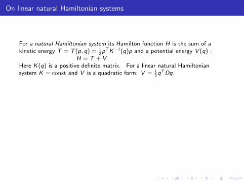
On linear natural Hamiltonian systems
For a natural Hamiltonian system its Hamilton function H is the sum of akinetic energy T = T (p, q) = 1
2pTK−1(q)p and a potential energy V (q) :
H = T + V .Here K(q) is a positive definite matrix. For a linear natural Hamiltoniansystem K = const and V is a quadratic form: V = 1
2qTDq.
TheoremIn any linear natural Hamiltonian system all non-zero eigenvalues are either realor pure imaginary. To each non-zero eigenvalue correspond only Jordan blocksof size 1. To zero eigenvalue correspond Jordan blocks of size 2.
Corollary
For linear natural Hamiltonian system collision of non-zero eigenvalues on theimaginary axis does not lead to a stability loss. Collision of eigenvalues at 0leads to the stability loss.
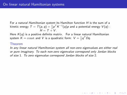
On linear natural Hamiltonian systems
For a natural Hamiltonian system its Hamilton function H is the sum of akinetic energy T = T (p, q) = 1
2pTK−1(q)p and a potential energy V (q) :
H = T + V .Here K(q) is a positive definite matrix. For a linear natural Hamiltoniansystem K = const and V is a quadratic form: V = 1
2qTDq.
TheoremIn any linear natural Hamiltonian system all non-zero eigenvalues are either realor pure imaginary. To each non-zero eigenvalue correspond only Jordan blocksof size 1. To zero eigenvalue correspond Jordan blocks of size 2.
Corollary
For linear natural Hamiltonian system collision of non-zero eigenvalues on theimaginary axis does not lead to a stability loss. Collision of eigenvalues at 0leads to the stability loss.
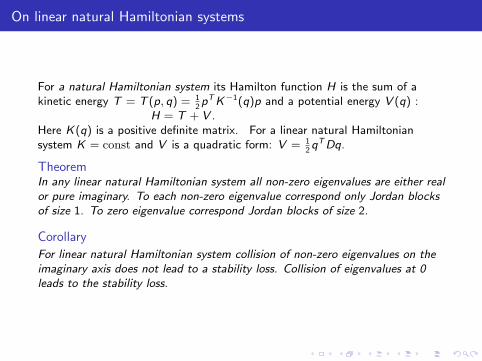
On linear natural Hamiltonian systems
For a natural Hamiltonian system its Hamilton function H is the sum of akinetic energy T = T (p, q) = 1
2pTK−1(q)p and a potential energy V (q) :
H = T + V .Here K(q) is a positive definite matrix. For a linear natural Hamiltoniansystem K = const and V is a quadratic form: V = 1
2qTDq.
TheoremIn any linear natural Hamiltonian system all non-zero eigenvalues are either realor pure imaginary. To each non-zero eigenvalue correspond only Jordan blocksof size 1. To zero eigenvalue correspond Jordan blocks of size 2.
Corollary
For linear natural Hamiltonian system collision of non-zero eigenvalues on theimaginary axis does not lead to a stability loss. Collision of eigenvalues at 0leads to the stability loss.
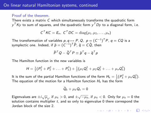
On linear natural Hamiltonian systems, continued
Proof of the theorem.There exists a matrix C which simultaneously transforms the quadratic formyTKy to sum of squares, and the quadratic form yTDy to a diagonal form, i.e.
CTKC = En, CTDC = diag(µ1, µ2, . . . , µn)
The transformation of variables p, q 7→ P, Q, p = (C−1)TP, q = CQ is asymplectic one. Indeed, if p = (C−1)T P, q = CQ, then
PTQ − QTP ≡ pTq − qTp
The Hamilton function in the new variables is
H = 12(P2
1 + P22 + . . . + P2
n ) + 12(µ1Q
21 + µ2Q
22 + . . . + µnQ
2n)
It is the sum of the partial Hamilton functions of the form Hk = 12(P2
k + µkQ2k ).
The equation of the motion for a Hamilton function Hk has the form
Qk + µkQk = 0
Eigenvalues are ±i√
µk, if µk > 0, and ±
√−µk , if µk < 0. Only for µk = 0 the
solution contains multiplier t, and so only to eigenvalue 0 there correspond theJordan block of the size 2.
Exercises
Exercises
1. Consider an equation x = v(t, x), x ∈ Rk . Prove that if divv ≡ 0, then theshift along trajectories of this equation preserves the standard phase volume inRk . (Hint: divv = tr(∂v/∂x).)
2. Give a geometric interpretation for skew-scalar product in the case of onedegree of freedom (n=1) and in the case of several degrees of freedom.
3. Obtain formulas for partial Hamilton functions corresponding to the pair ofa simple real eigenvalues (±a), to the quadruplet of a simple complexeigenvalues (±a± ib) and to the eigenvalue 0 of multiplicity 2 (a 6= 0, b 6= 0).

Periodic-coefficient linear Hamiltonian system.
Consider a periodic linear Hamiltonian system;
x = JA(t)x
where A(t) is a symmetric 2n × 2n matrix, A(t + T ) = A(t), A(·) ∈ C 0.
Let X (t) be the Cauchy fundamental matrix for this system (i.e. the columnsof X (t) are n linearly independent solutions to this system, X (0) = E2n).
We know that XT (t)JX (t) ≡ J. This implies that detX (t) ≡ 1.
Let Π be the monodromy matrix for this system. We know that Π = X (T ).Thus ΠTJΠ = J (so, Π is a symplectic matrix) and detΠ = 1
Periodic-coefficient linear Hamiltonian system, properties of multipliers
Recall the definition: Multipliers a eigenvalues of the monodromy matrix.
Proposition.
The matrix Π is similar to the matrix`Π−1
´T.
Proof.ΠTJΠ = J implies that
`Π−1
´T= JΠJ−1
Corollary
If ρ is a multiplier , then 1/ρ is a multiplier.Multipliers ρ and 1/ρ have equal multiplicities and the corresponding Jordanstructures in Π are the same.If ρ = −1 is a multiplier, then it necessarily has even multiplicity.If ρ = 1 is a multiplier, then it necessarily has even multiplicity.
Corollary
Characteristic polynomial d(ρ) = det(Π− ρE2n) of the matrix Π is aself-reciprocal (or, palindromic) one: d(1/ρ) = d(ρ)/ρ2n. So, the characteristicequation d(ρ) = 0 can be reduced to the form f (ρ + 1/ρ) = 0, where f (·) is apolynomial of degree n.
Periodic-coefficient linear Hamiltonian system, location of multipliers
TheoremMultipliers of a periodic-coefficient linear Hamiltonian system are situated onthe plane of complex variable symmetrically with respect to the unit circle (inthe sense of the inversion) and with respect to the real axis: if ρ is a multiplier,then 1/ρ, ρ, 1/ρ are also multipliers. The multipliers ρ, 1/ρ, ρ, 1/ρ have equalmultiplicities and the corresponding Jordan structures are the same.
So, multipliers may be of five types: real pairs (a, 1/a), pairs on the unit circlee iφ, e−iφ, quadruplets (a±1e±iφ), −1, and 1.
Corollary
If there is a simple eigenvalue on the unit circle, then it remains on the unitcircle under a small perturbation of the Hamiltonian. Similarly, a real simpleeigenvalue remains real under a small perturbation of the Hamiltonian.
So, the system may loss stability under a small perturbation of the Hamiltonianonly if there is a resonance.
When parameters of a stable periodic-coefficient linear Hamiltonian system arechanging, the multipliers move on the unit circle. When multipliers collide theymay leave the unit circle; this result in loss of stability. However, collision ofnot each pair of multipliers is dangerous, some multipliers necessarily passthrough each other without leaving the unit circle (M.G.Krein’s theory).

Bibliography
Arnold, V.I. Ordinary differential equations. Springer-Verlag, Berlin, 2006.
Arnold, V. I. Geometrical methods in the theory of ordinary differentialequations. Springer-Verlag, New York, 1988.
Arnold, V. I. Mathematical methods of classical mechanics. Springer-Verlag,New York, 1989. p
Coddington, E. A.; Levinson, N. Theory of ordinary differential equations.McGraw-Hill Book Company, Inc., New York-Toronto-London, 1955.
Dynamical systems. I, Encyclopaedia Math. Sci., 1, Springer-Verlag, Berlin,1998
Hartman, P. Ordinary differential equations. (SIAM), Philadelphia, PA, 2002.
Shilnikov, L. P.; Shilnikov, A. L.; Turaev, D. V.; Chua, L. O. Methods ofqualitative theory in nonlinear dynamics. Part I. World Scientific, Inc., RiverEdge, NJ, 1998.
Yakubovich, V. A.; Starzhinskii, V. M. Linear differential equations withperiodic coefficients. 1, 2. Halsted Press [John Wiley and Sons] NewYork-Toronto, 1975
LECTURE 6

LINEAR HAMILTONIAN SYSTEMS

List of formulas
A Hamiltonian system with a Hamilton function H is an ODE system of theform
p = −„
∂H
∂q
«T
, q =
„∂H
∂p
«T
Here p ∈ Rn, q ∈ Rn, p and q are considered as vector-columns, H is a functionof p, q, t, the superscript “T” denotes the matrix transposition. Components ofp are called “impulses”, components of q are called “coordinates”.
Let x be the vector-column combined of p and q. Then
x = J
„∂H
∂x
«T
, where J =
„0 −En
En 0
«The matrix J is called the symplectic unity. J2 = −E2n.
If H is a quadratic form, H = 12xTA(t)x , where A(t) is a symmetric 2n × 2n
matrix, A(·) ∈ C 0, then we get a linear Hamiltonian system
x = JA(t)x
List of formulas, continued
The skew-symmetric bilinear form [η, ξ] = ξTJη in R2n is called the skew-scalarproduct or the standard linear symplectic structure.
A 2n × 2n matrix M which satisfies the relation MTJM = J is called asymplectic matrix. A linear transformation of variables with a symplectic matrixis called a linear symplectic transformation of variables.
A linear transformations of variables is a symplectic transformations if and onlyif it preserves the skew-scalar product: [Mη, Mξ] = [η, ξ] for anyξ ∈ R2n, η ∈ R2n; here M is the matrix of the transformation.
The Cauchy fundamental matrix X (t) for a linear Hamiltonian system (i.e. thematrix X (t) such that its columns are n linearly independent solutions to thissystem, X (0) = E2n) is a symplectic matrix , i. e. XT (t)JX (t) = J for allt ∈ R.
For any linear T periodic ODE the matrix of the monodromy map is equal tothe value of Cauchy fundamental matrix X (t) at the moment of time T :Π = X (T ).
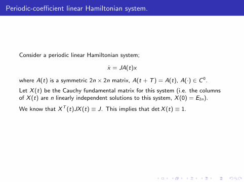
Periodic-coefficient linear Hamiltonian system.
Consider a periodic linear Hamiltonian system;
x = JA(t)x
where A(t) is a symmetric 2n × 2n matrix, A(t + T ) = A(t), A(·) ∈ C 0.
Let X (t) be the Cauchy fundamental matrix for this system (i.e. the columnsof X (t) are n linearly independent solutions to this system, X (0) = E2n).
We know that XT (t)JX (t) ≡ J. This implies that detX (t) ≡ 1.
Let Π be the monodromy matrix for this system. We know that Π = X (T ).Thus ΠTJΠ = J (so, Π is a symplectic matrix) and detΠ = 1
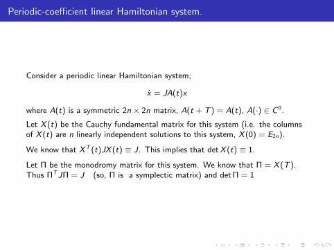

Periodic-coefficient linear Hamiltonian system, properties of multipliers
Recall the definition: Multipliers a eigenvalues of the monodromy matrix.
Proposition.
The matrix Π is similar to the matrix`Π−1
´T.
Proof.ΠTJΠ = J implies that
`Π−1
´T= JΠJ−1
Corollary
If ρ is a multiplier , then 1/ρ is a multiplier.Multipliers ρ and 1/ρ have equal multiplicities and the corresponding Jordanstructures in Π are the same.If ρ = −1 is a multiplier, then it necessarily has even multiplicity.If ρ = 1 is a multiplier, then it necessarily has even multiplicity.
Corollary
Characteristic polynomial d(ρ) = det(Π− ρE2n) of the matrix Π is aself-reciprocal (or, palindromic) one: d(1/ρ) = d(ρ)/ρ2n. So, the characteristicequation d(ρ) = 0 can be reduced to the form f (ρ + 1/ρ) = 0, where f (·) is apolynomial of degree n.
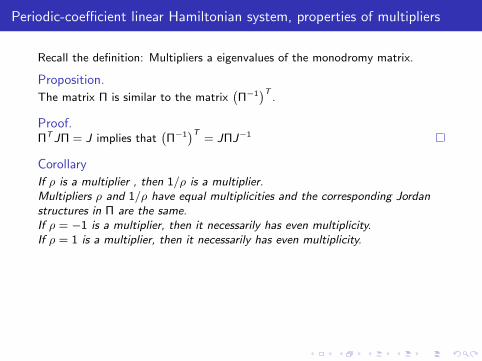
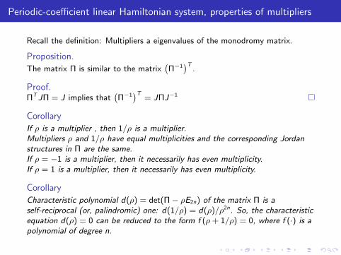

Periodic-coefficient linear Hamiltonian system, location of multipliers
TheoremMultipliers of a periodic-coefficient linear Hamiltonian system are situated onthe plane of complex variable symmetrically with respect to the unit circle (inthe sense of the inversion) and with respect to the real axis: if ρ is a multiplier,then 1/ρ, ρ, 1/ρ are also multipliers. The multipliers ρ, 1/ρ, ρ, 1/ρ have equalmultiplicities and the corresponding Jordan structures are the same.
So, multipliers may be of five types: real pairs (a, 1/a), pairs on the unit circlee iφ, e−iφ, quadruplets (a±1e±iφ), −1, and 1.
Corollary
If there is a simple eigenvalue on the unit circle, then it remains on the unitcircle under a small perturbation of the Hamiltonian. Similarly, a real simpleeigenvalue remains real under a small perturbation of the Hamiltonian.
So, the system may loss stability under a small perturbation of the Hamiltonianonly if there is a resonance.
When parameters of a stable periodic-coefficient linear Hamiltonian system arechanging, the multipliers move on the unit circle. When multipliers collide theymay leave the unit circle; this result in loss of stability. However, collision ofnot each pair of multipliers is dangerous, some multipliers necessarily passthrough each other without leaving the unit circle (M.G.Krein’s theory).
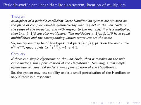
Periodic-coefficient linear Hamiltonian system, Krein’s theory
In the Krein’s theory each simple multiplier on the unit circle has a propertywhich is called the Krein signature.The Krein signature may be either positive or negative.If two multipliers on the unit circle with the same Krein signature collide, theypass through each other. If two multipliers on the unit circle with differentKrein signatures collide, they typically leave the unit circle; the multiplier withthe positive Krein signature is moving inside the unit circle, and the multiplierwith the negative Krein signature is moving outside the unit circle.
One can distinguish multipliers with different Krein signatures on the basis ofthe following test:Consider perturbed system
x = J(A(t) + δB(t))x
B(t) is a symmetric positive-definite 2n × 2n matrix, B(t + T ) = B(t),0 < δ 1.
Theorem (Krein’s test)
For small enough δ, when δ groves, on the unit circle multipliers with thepositive signature move counterclockwise, and multipliers with the negativesignature move clockwise.
Parametric resonance
Consider a periodic-coefficient linear Hamiltonian system which is a smalltime-periodic perturbation of a stable constant-coefficient Hamiltonian system:
x = J(A + εB(t))x
where A and B(t) are a symmetric 2n × 2n matrices, B(t + T ) = B(t),B(·) ∈ C 0, 0 < ε 1.
We assume that the eigenvalues of JA are different purely imaginary numbers±iω1,±iω2, . . . ,±iωn. This guarantees stability of the unperturbed system.Values |ω1|, |ω2|, . . . , |ωn| are the eigen-frequencies of the unperturbed system.
If B were constant, then the system would be stable provided that ε is smallenough. It turns out that the system can be made unstable by an arbitrarysmall periodic perturbation of an appropriate period T . This phenomenon iscalled the parametric resonance. The necessary condition for the parametricresonance is that the unperturbed system considered as T -periodic systemhas non-simple multipliers.
The multipliers are e±iω1T , e±iω2T , . . . , e±iωnT . So, in the case of a parametricresonance e±iωjT = e±iωmT for some j , m. This implies that±ωjT = ±ωmT + 2πk for a certain integer k. For j = m we get ωm = k
22πT
.
Parametric resonance, application of the Krein theory
Let the normal form of the Hamiltonian function for the Hamiltonian systemx = JAx be
H = 12Ω1(p
21 + q2
1) + 12Ω2(p
22 + q2
2) + . . . + 12Ωn(p
2n + q2
n)
Then eigenvalues of the matrix JA are ±iΩ1, ±iΩ2, . . . , ±iΩn.Consider Hamiltonian system whose Hamiltonian in the variables p, q is
F = H + 12δ(p2
1 + q21 + p2
2 + q22 + . . . + p2
n + q2n)
The eigenvalues of the matrix of this Hamiltonian system are± i(Ω1 + δ), ±i(Ω2 + δ), . . . , ±i(Ωn + δ).
The eigenvalues of the monodromy matrix for the time T aree±i(Ω1+δ)T , e±i(Ω2+δ)T , . . . , e±i(Ωn+δ)T .
According to the Krein test, when δ grows, the multipliers with the positiveKrein signature should move counterclockwise, and multipliers with thenegative signature should move clockwise. Therefore, here multipliers with thesign “+” in the exponent have positive Krein signature, and those with thesign “-” have negative Krein signature.Thus, if a relation e iΩjT = e iΩmT for some j , m is satisfied, then a T -periodicperturbation can not destroy stability (there is no parametric resonance). Inopposite, if a relation e iΩjT = e−iΩmT for some j , m is satisfied, then thereexists a T -periodic perturbation that destroy stability, i.e. leads to a parametricresonance.
Symplectic version of Floquet-Lyapunov theory
TheoremA linear Hamiltonian system that is T -periodic in time can be reduced to anautonomous form by a linear symplectic transformation of variables. If thesystem has no negative real multipliers, then the reducing transformation ofvariables can be chosen to be T-periodic in time, and if the system hasnegative real multipliers, then 2T-periodic. If the system depends smoothly ona parameter, then the transformation of variables can also be chosen to besmooth in this parameter.
RemarkLet a periodic-coefficient linear Hamiltonian system has the form
x = J(A + εB(t, ε))xwith a smooth dependence of B on ε. Then, according to the previous theoremit can be reduced to an autonomous system
y = J(A0 + εA1(ε))yHowever, it can happens that the reducing transformation is not close to theautonomous one and A0 6= A. The reason is similar to that for a parametricresonance. It can happens that the matrix A has simple eigenvalues λ1 and λ2
such that λ2 − λ1 = 2πiT
m with an integer m. Then for ε = 0 the monodromy
matrix Π = eTA has the eigenvalue (the multiplier) eTλ1 of multiplicity 2.
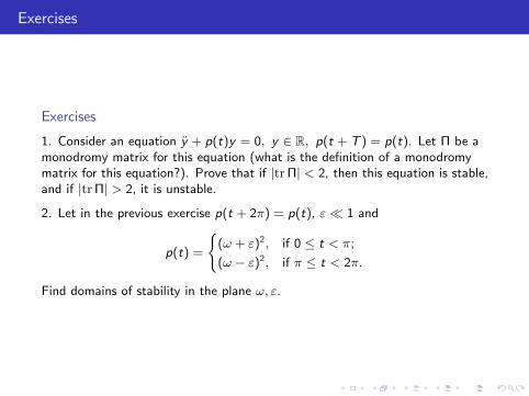
Exercises
Exercises
1. Consider an equation y + p(t)y = 0, y ∈ R, p(t + T ) = p(t). Let Π be amonodromy matrix for this equation (what is the definition of a monodromymatrix for this equation?). Prove that if |tr Π| < 2, then this equation is stable,and if |tr Π| > 2, it is unstable.
2. Let in the previous exercise p(t + 2π) = p(t), ε 1 and
p(t) =
((ω + ε)2, if 0 ≤ t < π;
(ω − ε)2, if π ≤ t < 2π.
Find domains of stability in the plane ω, ε.

LINEARISATION
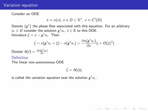
Variation equation
Consider an ODE
x = v(x), x ∈ D ⊂ Rn, v ∈ C 2(D)
Denote g t the phase flow associated with this equation. For an arbitraryx∗ ∈ D consider the solution g tx∗, t ∈ R to this ODE.Introduce ξ = x − g tx∗. Then
ξ = v(g tx∗ + ξ)− v(g tx∗) =∂v(g tx∗)
∂xξ + O(|ξ|2)
Denote A(t) = ∂v(g tx∗)∂x
DefinitionThe linear non-autonomous ODE
ξ = A(t)ξ
is called the variation equation near the solution g tx∗.
Denote ϕ(t) = dg tx∗dt
.
Proposition.
ϕ(t) is a solution to the variation equation.
Proof.ϕ = d
dt( dg tx∗
dt) = d
dtv(g tx∗) = ∂v(g tx∗)
∂xdg tx∗
dt= A(t)ϕ
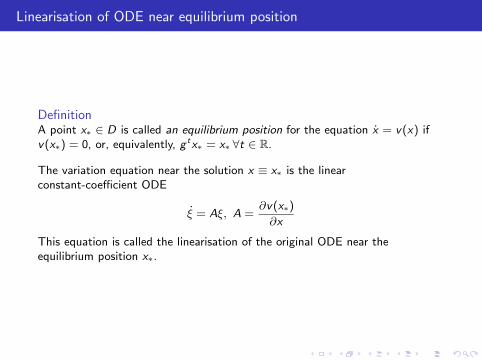
Linearisation of ODE near equilibrium position
DefinitionA point x∗ ∈ D is called an equilibrium position for the equation x = v(x) ifv(x∗) = 0, or, equivalently, g tx∗ = x∗ ∀t ∈ R.
The variation equation near the solution x ≡ x∗ is the linearconstant-coefficient ODE
ξ = Aξ, A =∂v(x∗)
∂x
This equation is called the linearisation of the original ODE near theequilibrium position x∗.
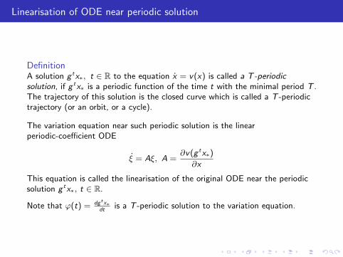
Linearisation of ODE near periodic solution
DefinitionA solution g tx∗, t ∈ R to the equation x = v(x) is called a T-periodicsolution, if g tx∗ is a periodic function of the time t with the minimal period T .The trajectory of this solution is the closed curve which is called a T -periodictrajectory (or an orbit, or a cycle).
The variation equation near such periodic solution is the linearperiodic-coefficient ODE
ξ = Aξ, A =∂v(g tx∗)
∂x
This equation is called the linearisation of the original ODE near the periodicsolution g tx∗, t ∈ R.
Note that ϕ(t) = dg tx∗dt
is a T -periodic solution to the variation equation.

Normal coordinates in a neighborhood of periodic trajectory
TheoremIn a small neighborhood of any periodic trajectory there exists a transformationof variables x 7→ (y , θ), y ∈ Rn−1, θ ∈ S1 such that the system takes the form
y = u(y , θ), u(0, θ) ≡ 0
θ = ω + w(y , θ), ω = const > 0, w(0, θ) ≡ 0
The variables y in such representation are called normal variables. The periodictrajectory has the equation y = 0 and is parametrized by the angle θ.
Variation equation near periodic trajectory in normal coordinates
Using normal coordinates in a neighborhood of a periodic trajectory with θ asthe new time leads to the equation
dy
dθ=
1
ωu(y , θ) + O(|y |2)
Denote B(θ) = 1ω
∂u(0,θ)∂y
.
DefinitionThe linear 2π-periodic ODE
dy
dθ= B(θ)y
is called the linearisation, or the variation equation, of the original ODE nearthe periodic trajectory in the normal coordinates.
According to Floquet-Lyapunov theory this ODE can be transformed into anautonomous ODE by a linear 2π- or 4π-periodic in θ transformation ofvariables.

LECTURE 7
LINEARISATION

Variation equation
Consider an ODE
x = v(x), x ∈ D ⊂ Rn, v ∈ C 2(D)
Denote g t the phase flow associated with this equation. For an arbitraryx∗ ∈ D consider the solution g tx∗, t ∈ R to this ODE.Introduce ξ = x − g tx∗. Then
ξ = v(g tx∗ + ξ)− v(g tx∗) =∂v(g tx∗)
∂xξ + O(|ξ|2)
Denote A(t) = ∂v(g tx∗)∂x
DefinitionThe linear non-autonomous ODE
ξ = A(t)ξ
is called the variation equation near the solution g tx∗.
Denote ϕ(t) = dg tx∗dt
.
Proposition.
ϕ(t) is a solution to the variation equation.
Proof.ϕ = d
dt( dg tx∗
dt) = d
dtv(g tx∗) = ∂v(g tx∗)
∂xdg tx∗
dt= A(t)ϕ
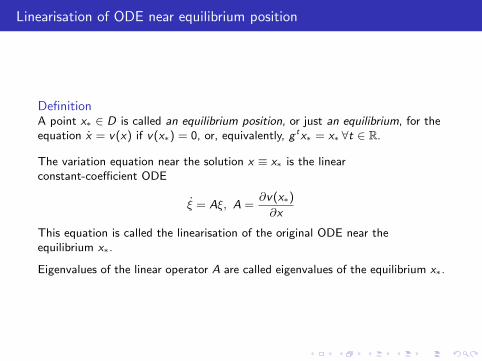
Linearisation of ODE near equilibrium position
DefinitionA point x∗ ∈ D is called an equilibrium position, or just an equilibrium, for theequation x = v(x) if v(x∗) = 0, or, equivalently, g tx∗ = x∗ ∀t ∈ R.
The variation equation near the solution x ≡ x∗ is the linearconstant-coefficient ODE
ξ = Aξ, A =∂v(x∗)
∂x
This equation is called the linearisation of the original ODE near theequilibrium x∗.
Eigenvalues of the linear operator A are called eigenvalues of the equilibrium x∗.
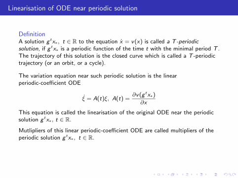
Linearisation of ODE near periodic solution
DefinitionA solution g tx∗, t ∈ R to the equation x = v(x) is called a T-periodicsolution, if g tx∗ is a periodic function of the time t with the minimal period T .The trajectory of this solution is the closed curve which is called a T -periodictrajectory (or an orbit, or a cycle).
The variation equation near such periodic solution is the linearperiodic-coefficient ODE
ξ = A(t)ξ, A(t) =∂v(g tx∗)
∂x
This equation is called the linearisation of the original ODE near the periodicsolution g tx∗, t ∈ R.
Mutlipliers of this linear periodic-coefficient ODE are called multipliers of theperiodic solution g tx∗, t ∈ R.
Note that ϕ(t) = dg tx∗dt
is a T -periodic solution to the variation equation.
Thus, periodic solution always have 1 as a multiplier.
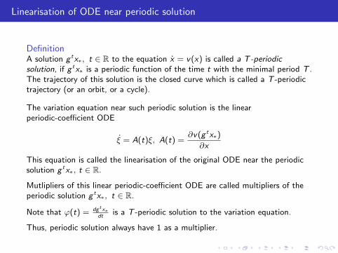
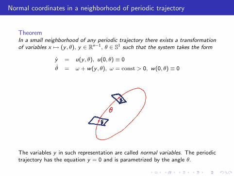
Normal coordinates in a neighborhood of periodic trajectory
TheoremIn a small neighborhood of any periodic trajectory there exists a transformationof variables x 7→ (y , θ), y ∈ Rn−1, θ ∈ S1 such that the system takes the form
y = u(y , θ), u(0, θ) ≡ 0
θ = ω + w(y , θ), ω = const > 0, w(0, θ) ≡ 0
The variables y in such representation are called normal variables. The periodictrajectory has the equation y = 0 and is parametrized by the angle θ.
Variation equation near periodic trajectory in normal coordinates
Using normal coordinates in a neighborhood of a periodic trajectory with θ asthe new time leads to the equation
dy
dθ=
1
ωu(y , θ) + O(|y |2)
Denote B(θ) = 1ω
∂u(0,θ)∂y
.
DefinitionThe linear 2π-periodic ODE
dy
dθ= B(θ)y
is called the linearisation, or the variation equation, of the original ODE nearthe periodic trajectory in the normal coordinates.
According to Floquet-Lyapunov theory this ODE can be transformed into anautonomous ODE by a linear 2π- or 4π-periodic in θ transformation ofvariables.
Multipliers of the variation equation near the periodic trajectory in the normalcoordinates are called multipliers of the periodic trajectory. (Note: thismultipliers are also multipliers of corresponding periodic solution, which havealso 1 as the multiplier.)
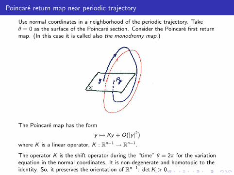
Poincare return map near periodic trajectory
Use normal coordinates in a neighborhood of the periodic trajectory. Takeθ = 0 as the surface of the Poincare section. Consider the Poincare first returnmap. (In this case it is called also the monodromy map.)
The Poincare map has the form
y 7→ Ky + O(|y |2)where K is a linear operator, K : Rn−1 → Rn−1.
The operator K is the shift operator during the “time” θ = 2π for the variationequation in the normal coordinates. It is non-degenerate and homotopic to theidentity. So, it preserves the orientation of Rn−1: det K > 0.
Linearisation of map near fixed point
Consider a mapP : D → D, D ⊂ Rn, P ∈ C 2(D)
This map sends a point x to a point P(x).
DefinitionThe point x∗ ∈ D is called a fixed point of the map P if P(x∗) = x∗.
Introduce ξ = x − x∗. Then
x∗ + ξ 7→ P(x∗ + ξ) = x∗ +∂P(x∗)
∂xξ + O(|ξ|2)
Denote A = ∂P(x∗)∂x
DefinitionThe linear map
ξ 7→ Aξ
is called the linearisation of the original map P near the fixed point x∗.
The eigenvalues of the operator A are called the multipliers of the fixed pointx∗.
Multipliers of the fixed point of Poincare return map near a periodic trajectorycoincide with the defined earlier mutipliers of this periodic trajectory.
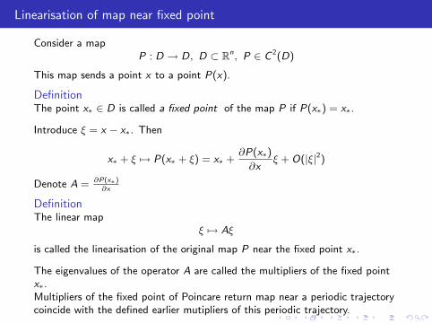
Linearisation of map near fixed point
Consider a mapP : D → D, D ⊂ Rn, P ∈ C 2(D)
This map sends a point x to a point P(x).
DefinitionThe point x∗ ∈ D is called a fixed point of the map P if P(x∗) = x∗.
Introduce ξ = x − x∗. Then
x∗ + ξ 7→ P(x∗ + ξ) = x∗ +∂P(x∗)
∂xξ + O(|ξ|2)
Denote A = ∂P(x∗)∂x
DefinitionThe linear map
ξ 7→ Aξ
is called the linearisation of the original map P near the fixed point x∗.
The eigenvalues of the operator A are called the multipliers of the fixed pointx∗.Multipliers of the fixed point of Poincare return map near a periodic trajectorycoincide with the defined earlier mutipliers of this periodic trajectory.
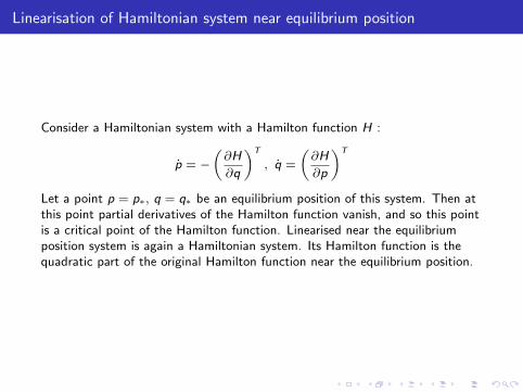
Linearisation of Hamiltonian system near equilibrium position
Consider a Hamiltonian system with a Hamilton function H :
p = −„
∂H
∂q
«T
, q =
„∂H
∂p
«T
Let a point p = p∗, q = q∗ be an equilibrium position of this system. Then atthis point partial derivatives of the Hamilton function vanish, and so this pointis a critical point of the Hamilton function. Linearised near the equilibriumposition system is again a Hamiltonian system. Its Hamilton function is thequadratic part of the original Hamilton function near the equilibrium position.
Linearisation of Hamiltonian system near periodic trajectory
Suppose that an autonomous Hamiltonian system in R2n has a periodictrajectory which is not an equilibrium position. Such trajectories are notisolated but, as a rule, form families.
Proposition.In a neighbourhood of a periodic trajectory there exist new symplecticcoordinates θ mod 2π, I ∈ R1 and z ∈ R2(n−1), such that I = 0 and z = 0 onthe trajectory under consideration, and going around this trajectory changes θby 2π; on the trajectory itself θ = Ω = const > 0. In the new coordinates theHamiltonian function takes the form H = ΩI +H(z , θ, I ) , where the expansionof H in z , I begins with terms of the second order of smallness.
Perform the isoenergetic reduction (also called Whittaker transformation)choosing, on each energy level H = h close to the original one, the phase θ forthe new time. The Hamiltonian of the problem takes the form F = F (z , θ, h).For h = 0 the origin is an equilibrium position of the system. Suppose thatthis equilibrium position is non-degenerate. Then for small h the system has anon-degenerate periodic solution. By a change of variables smooth in theparameter one can shift origin of coordinates to this periodic solution. TheHamiltonian takes the form
F = 12zTA(θ, h)z + G(z , θ, h)
where the expansion of G in z begins with terms of the third order ofsmallness; the Hamiltonian has period 2π in θ.
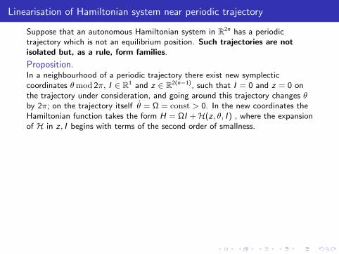
Linearisation of Hamiltonian system near periodic trajectory
Suppose that an autonomous Hamiltonian system in R2n has a periodictrajectory which is not an equilibrium position. Such trajectories are notisolated but, as a rule, form families.
Proposition.In a neighbourhood of a periodic trajectory there exist new symplecticcoordinates θ mod 2π, I ∈ R1 and z ∈ R2(n−1), such that I = 0 and z = 0 onthe trajectory under consideration, and going around this trajectory changes θby 2π; on the trajectory itself θ = Ω = const > 0. In the new coordinates theHamiltonian function takes the form H = ΩI +H(z , θ, I ) , where the expansionof H in z , I begins with terms of the second order of smallness.
Perform the isoenergetic reduction (also called Whittaker transformation)choosing, on each energy level H = h close to the original one, the phase θ forthe new time. The Hamiltonian of the problem takes the form F = F (z , θ, h).For h = 0 the origin is an equilibrium position of the system.
Suppose thatthis equilibrium position is non-degenerate. Then for small h the system has anon-degenerate periodic solution. By a change of variables smooth in theparameter one can shift origin of coordinates to this periodic solution. TheHamiltonian takes the form
F = 12zTA(θ, h)z + G(z , θ, h)
where the expansion of G in z begins with terms of the third order ofsmallness; the Hamiltonian has period 2π in θ.
Linearisation of Hamiltonian system near periodic trajectory
Suppose that an autonomous Hamiltonian system in R2n has a periodictrajectory which is not an equilibrium position. Such trajectories are notisolated but, as a rule, form families.
Proposition.In a neighbourhood of a periodic trajectory there exist new symplecticcoordinates θ mod 2π, I ∈ R1 and z ∈ R2(n−1), such that I = 0 and z = 0 onthe trajectory under consideration, and going around this trajectory changes θby 2π; on the trajectory itself θ = Ω = const > 0. In the new coordinates theHamiltonian function takes the form H = ΩI +H(z , θ, I ) , where the expansionof H in z , I begins with terms of the second order of smallness.
Perform the isoenergetic reduction (also called Whittaker transformation)choosing, on each energy level H = h close to the original one, the phase θ forthe new time. The Hamiltonian of the problem takes the form F = F (z , θ, h).For h = 0 the origin is an equilibrium position of the system. Suppose thatthis equilibrium position is non-degenerate. Then for small h the system has anon-degenerate periodic solution. By a change of variables smooth in theparameter one can shift origin of coordinates to this periodic solution. TheHamiltonian takes the form
F = 12zTA(θ, h)z + G(z , θ, h)
where the expansion of G in z begins with terms of the third order ofsmallness; the Hamiltonian has period 2π in θ.
Linearisation of Hamiltonian system near periodic trajectory, continued
Symplectic version of the Floquet-Lyapunov theory allows to reduce theproblem to the case when the quadratic part of the Hamiltonian does notdepend on θ:
F = 12zT A(h)z + G(z , θ, h) .
Exercises
Exercises
1. Prove that multipliers of a periodic trajectory coincide with multipliers ofthe fixed point of the corresponding Poincare return map.
2. Let for isoenergetic reduction procedure some coordinate is introduced asthe new time. Proof that the new Hamilton function is the impulse conjugatedto this coordinate, expressed through value of energy and remaining phasevariables and taken with the sign ”-”.
LOCAL TOPOLOGICAL EQUIVALENCE
TO LINEAR SYSTEM

Definition of topological equivalence
DefinitionTwo dynamical systems with phase spaces X1 ⊆ Rn and X2 ⊆ Rn aretopologically equivalent in the domains U1 ⊆ X1, U2 ⊆ X2 if there exists ahomeomorphism η : U1 → U2 which maps trajectories, half-trajectories,segments of trajectories of the first system to trajectories, half-trajectories,segments of trajectories of the second system preserving the direction of time.
For dynamical systems with discrete time the topological equivalency isequivalent to the topological conjugacy of evolutionary operators for time 1.
DefinitionTwo diffeomorphisms, g1 and g2, which are defined in the domains X1 ⊆ Rn
and X2 ⊆ Rn respectively, are topologically conjugate in the domainsU1 ⊆ X1, U2 ⊆ X2 if there exists a homeomorphism η : U1 → U2 such thatη(g1(x)) = g2(η(x)) for any x ∈ U1.
If g1 and g2 are topologically conjugate then we have the commutative diagram:
−−−−−→ U1g1−−−−−→ U1
g1−−−−−→ U1 −−−−−→??yη
??yη
??yη
−−−−−→ U2g2−−−−−→ U2
g2−−−−−→ U2 −−−−−→
Local topological equivalence to linearisation
A question about local topological equivalence to linearisation make sense onlyfor neighborhoods of equilibria without eigenvalues on imaginary axis, forperiodic trajectories (fixed points of maps) without multipliers on the unitcircle.
DefinitionAn equilibrium position of an ODE is called hyperbolic if it does not haveeigenvalues on the imaginary axis.A periodic trajectory of an ODE is called hyperbolic if it does not havemultipliers on the unit circle.A fixed point of a map is called hyperbolic if it does not have multipliers on theunit circle.
Bibliography
Arnold, V.I. Ordinary differential equations. Springer-Verlag, Berlin, 2006.
Arnold, V. I. Geometrical methods in the theory of ordinary differentialequations. Springer-Verlag, New York, 1988.
Arnold, V. I. Mathematical methods of classical mechanics. Springer-Verlag,New York, 1989.
Arrowsmith, D. , Place, C. An introduction to dynamical systems, CambridgeUniversity Press, Cambridge, 1990.
Dynamical systems. I, Encyclopaedia Math. Sci., 1, Springer-Verlag, Berlin,1998.
Guckenheimer, J. Holmes, P . Nonlinear oscillations, dynamical systems andbifurcations of vector fields, Springer-Verlag, Berlin, 1990.
Ilyashenko, Yu., Weigu Li, Nonlocal Bifurcations , AMS, 1999.
Hartman, P. Ordinary differential equations. (SIAM), Philadelphia, PA, 2002.
Kuznetsov, Yu.A. Elements of applied bifurcation theory. Springer-Verlag, NewYork, 2004.
Shilnikov, L. P.; Shilnikov, A. L.; Turaev, D. V.; Chua, L. O. Methods ofqualitative theory in nonlinear dynamics. Part I. World Scientific, Inc., RiverEdge, NJ, 1998.
LECTURE 8

LOCAL TOPOLOGICAL EQUIVALENCE
TO LINEAR SYSTEM
Definition of topological equivalence
DefinitionTwo dynamical systems with phase spaces X1 ⊆ Rn and X2 ⊆ Rn aretopologically equivalent in the domains U1 ⊆ X1, U2 ⊆ X2 if there exists ahomeomorphism η : U1 → U2 which maps trajectories, half-trajectories,segments of trajectories of the first system to trajectories, half-trajectories,segments of trajectories of the second system preserving the direction of time.
For dynamical systems with discrete time the topological equivalency isequivalent to the topological conjugacy of evolutionary operators for time 1.
DefinitionTwo diffeomorphisms, g1 and g2, which are defined in the domains X1 ⊆ Rn
and X2 ⊆ Rn respectively, are topologically conjugate in the domainsU1 ⊆ X1, U2 ⊆ X2 if there exists a homeomorphism η : U1 → U2 such thatη(g1(x)) = g2(η(x)) for any x ∈ U1.
If g1 and g2 are topologically conjugate then we have the commutative diagram:
−−−−−→ U1g1−−−−−→ U1
g1−−−−−→ U1 −−−−−→??yη
??yη
??yη
−−−−−→ U2g2−−−−−→ U2
g2−−−−−→ U2 −−−−−→

Local topological equivalence to linearisation
A question about local topological equivalence to linearisation make sense onlyfor neighborhoods of equilibria without eigenvalues on imaginary axis, forperiodic trajectories (fixed points of maps) without multipliers on the unitcircle.
DefinitionAn equilibrium position of an ODE is called hyperbolic if it does not haveeigenvalues on the imaginary axis.A periodic trajectory of an ODE is called hyperbolic if it does not havemultipliers on the unit circle.A fixed point of a map is called hyperbolic if it does not have multipliers on theunit circle.
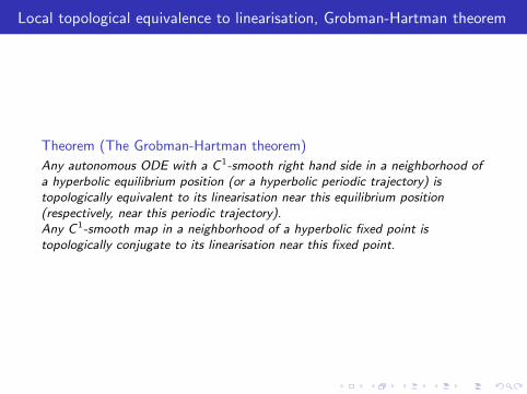
Local topological equivalence to linearisation, Grobman-Hartman theorem
Theorem (The Grobman-Hartman theorem)
Any autonomous ODE with a C 1-smooth right hand side in a neighborhood ofa hyperbolic equilibrium position (or a hyperbolic periodic trajectory) istopologically equivalent to its linearisation near this equilibrium position(respectively, near this periodic trajectory).Any C 1-smooth map in a neighborhood of a hyperbolic fixed point istopologically conjugate to its linearisation near this fixed point.
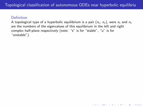
Topological classification of autonomous ODEs near hyperbolic equilibria
DefinitionA topological type of a hyperbolic equilibrium is a pair (ns , nu), were ns and nu
are the numbers of the eigenvalues of this equilibrium in the left and rightcomplex half-plane respectively (note: “s” is for “stable”, “u” is for“unstable”).
TheoremLinear (hyperbolic) autonomous ODEs in Rn of the same topological type aretopologically equivalent.
Corollary
Any autonomous ODE in Rn with a C 1-smooth right hand side in aneighborhood of a hyperbolic equilibrium position of a topological type (ns , nu)is topologically equivalent to the system of linear ODEs
ξ = −ξ, ξ ∈ Rns , η = η, η ∈ Rnu
A hyperbolic equilibrium position of a topological type (ns , nu) is called atopological saddle if both ns and nu are different from 0. It is called a stable(respectively, unstable) topological node if nu = 0 (respectively, ns = 0).
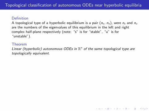
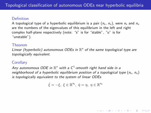
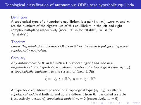
Topological classification of maps near hyperbolic fixed points
DefinitionA topological type of a hyperbolic fixed point of a map is a quadruple(ns , δs , nu, δu), were ns and nu are the numbers of the multipliers of this fixedpoint inside and outside of the unit circle respectively, δs and δu are signs ofproducts of these multipliers.
TheoremLinear (hyperbolic) maps in Rn of the same topological type are topologicallyconjugate.
Corollary
Any C 1-smooth hyperbolic map in Rn in a neighborhood of a hyperbolic fixedpoint of a topological type (ns , δs , nu, δu) is topologically conjugate to thelinear map
ξ 7→ Asξ, ξ ∈ Rns , η 7→ Auη, η ∈ Rnu ,where As is the diagonal matrix with all diagonal elements equal to 1/2 but thelast one which is equal to δs/2, and Au is the diagonal matrix with all diagonalelements equal to 2 but the last one which is equal to 2δu.
For the linear maps above the plane η = 0 is called the stable plane, and theplane ξ = 0 is called the unstable plane. The maps with δs = −1,(respectively, with δu = −1) change the orientation of the stable (respectively,unstable) plane.The maps with different topological types are topologically not equivalent.
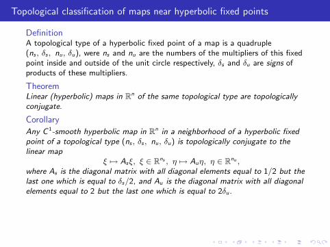
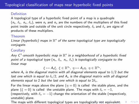
Topological classification of ODEs near hyperbolic periodic trajectories
ODEs near hyperbolic periodic trajectories are topologically equivalent if andonly if the corresponding monodromy maps are topologically equivalent.
Because any monodromy map in Rn preserves the orientation of Rn, for suchmap necessarily δsδu = 1. So, for given (ns , nu) there are two topologicallynon-equivalent classes of ODEs near hyperbolic periodic trajectories.
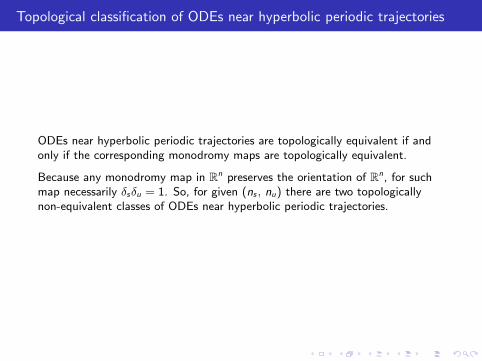
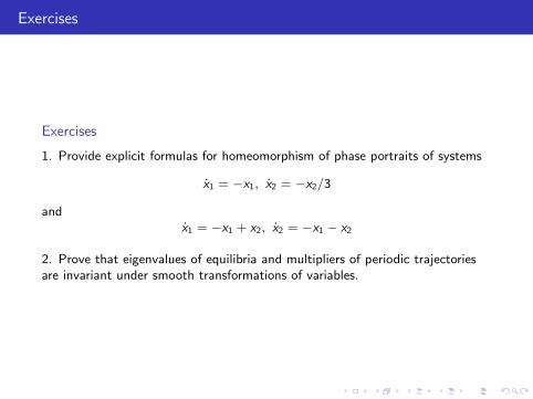
Exercises
Exercises
1. Provide explicit formulas for homeomorphism of phase portraits of systems
x1 = −x1, x2 = −x2/3
andx1 = −x1 + x2, x2 = −x1 − x2
2. Prove that eigenvalues of equilibria and multipliers of periodic trajectoriesare invariant under smooth transformations of variables.
LOCAL INVARIANT MANIFOLDS

Stable and unstable invariant manifolds
DefinitionA manifold is called an invariant manifold for a dynamical system if thismanifold together with each its point contains the whole trajectory of thisdynamical system.
Example
Consider the linear system
ξ = −ξ, ξ ∈ Rns , η = η, η ∈ Rnu
It has two invariant planes: plane η = 0 is called the stable plane, and theplane ξ = 0 is called the unstable plane; trajectories in these planesexponentially fast tend to the origin of the coordinates as t → +∞ andt → −∞ respectively. Similarly, one can define the stable and the unstableplanes T s and T u for any hyperbolic linear system.
Stable and unstable manifolds of hyperbolic equilibria, periodic trajectoriesand fixed points
Consider an ODEx = Ax + O(|x |2), x ∈ Rn
with the right hand side of smoothness C r (here one can consider also r = ∞and r = ω; the last notation is for the class of analytic functions). Assume thatthe matrix A has ns and nu eigenvalues in the left and right complex half-planerespectively, ns + nu = n. Denote T s and T u the corresponding invariantplanes of A.
Theorem (The Hadamard-Perron theorem)
In some neighborhood of the origin this ODE has two C r -smooth invariantmanifolds W s and W u, which are tangent at the origin to the planes T s andT u respectively. Trajectories in these manifolds exponentially fast tend to theorigin of the coordinates as t → +∞ and t → −∞ respectively. W s and W u
are called stable and unstable manifolds of the equilibrium 0 respectively.
RemarkFor analytic systems this result was obtained by A.M.Lyapunov and A.Poincare.
Similar theorem is valid for maps in neighborhoods of hyperbolic fixed pointsand for ODEs in neighborhoods of hyperbolic periodic trajectories.
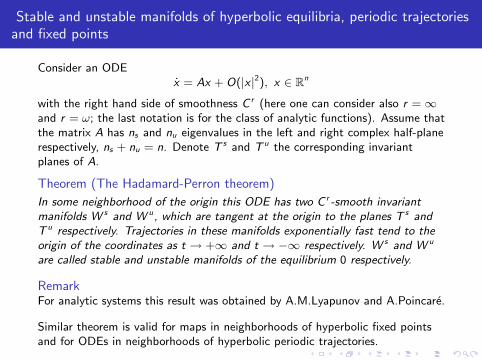
LECTURE 9

LOCAL INVARIANT MANIFOLDS
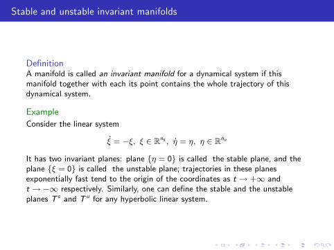
Stable and unstable invariant manifolds
DefinitionA manifold is called an invariant manifold for a dynamical system if thismanifold together with each its point contains the whole trajectory of thisdynamical system.
Example
Consider the linear system
ξ = −ξ, ξ ∈ Rns , η = η, η ∈ Rnu
It has two invariant planes: plane η = 0 is called the stable plane, and theplane ξ = 0 is called the unstable plane; trajectories in these planesexponentially fast tend to the origin of the coordinates as t → +∞ andt → −∞ respectively. Similarly, one can define the stable and the unstableplanes T s and T u for any hyperbolic linear system.
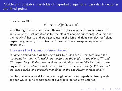
Stable and unstable manifolds of hyperbolic equilibria, periodic trajectoriesand fixed points
Consider an ODEx = Ax + O(|x |2), x ∈ Rn
with the right hand side of smoothness C r (here one can consider also r = ∞and r = ω; the last notation is for the class of analytic functions). Assume thatthe matrix A has ns and nu eigenvalues in the left and right complex half-planerespectively, ns + nu = n. Denote T s and T u the corresponding invariantplanes of A.
Theorem (The Hadamard-Perron theorem)
In some neighborhood of the origin this ODE has two C r -smooth invariantmanifolds W s and W u, which are tangent at the origin to the planes T s andT u respectively. Trajectories in these manifolds exponentially fast tend to theorigin of the coordinates as t → +∞ and t → −∞ respectively. W s and W u
are called stable and unstable manifolds of the equilibrium 0 respectively.
Similar theorem is valid for maps in neighborhoods of hyperbolic fixed pointsand for ODEs in neighborhoods of hyperbolic periodic trajectories.
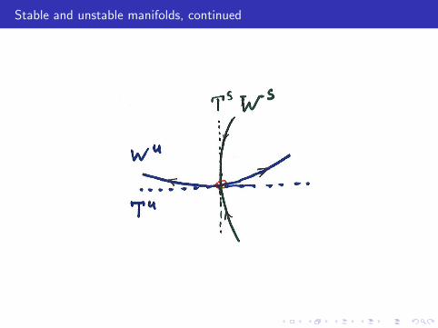
Stable and unstable manifolds, continued
The center manifold theorem
Consider an ODEx = Ax + O(|x |2), x ∈ Rn
with the right hand side of smoothness C r , r < ∞. Assume that the matrix Ahas ns , nu and nc eigenvalues in the left complex half-plane, right complexhalf-plane and on imaginary axis respectively, ns + nu + nc = n. Denote T s , T u
and T c the corresponding invariant planes of A . (Note: “s” is for “stable”,“u” is for “unstable”, “c” is for “center ”).
Theorem (The center manifold theorem: Pliss-Kelley-Hirsch-Pugh-Shub)
In some neighborhood U of the origin this ODE has C r -smooth invariantmanifolds W s , W u and C r−1-smooth invariant manifold W c , which aretangent at the origin to the planes T s , T u and T c respectively. Trajectories inthe manifolds W s and W u exponentially fast tend to the origin as t → +∞and t → −∞ respectively. Trajectories which remain in U for all t ≥ 0 (t ≤ 0)tend to W c as t → +∞ (t → −∞). W s , W u and W c are called the stable,the unstable and a center manifolds of the equilibrium 0 respectively.
RemarkBehavior of trajectories on W c is determined by nonlinear terms.
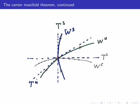
The center manifold theorem, continued
The center manifold theorem, continued
RemarkIf the original equation has smoothness C∞ or Cω, then W s and W u also havesmoothness C∞ or Cω. However W c in general has only a finite smoothness.
RemarkIf ns = 0 or nu = 0 and the original equation has smoothness C r , r < ∞ , thenW c has smoothness C r .
The center manifold theorem, examples
Example (A center manifold need not be unique)
x = x2, y = −y
Example (A center manifold in general has only finite smoothness)
x = xz − x3, y = y + x4, z = 0
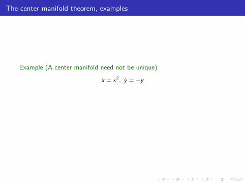
The center manifold theorem, examples
Example (A center manifold need not be unique)
x = x2, y = −y
Example (A center manifold in general has only finite smoothness)
x = xz − x3, y = y + x4, z = 0
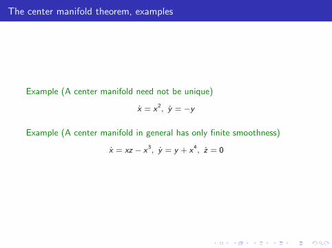
The center manifold theorem, examples
Example (A center manifold need not be unique)
x = x2, y = −y
Example (A center manifold in general has only finite smoothness)
x = xz − x3, y = y + x4, z = 0
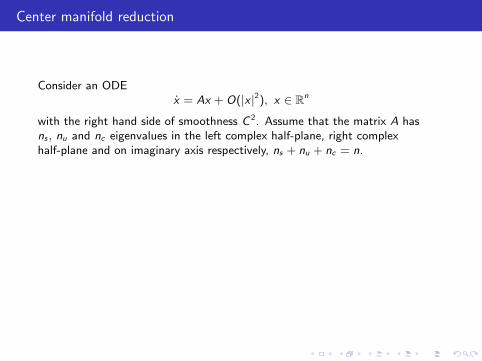
Center manifold reduction
Consider an ODEx = Ax + O(|x |2), x ∈ Rn
with the right hand side of smoothness C 2. Assume that the matrix A hasns , nu and nc eigenvalues in the left complex half-plane, right complexhalf-plane and on imaginary axis respectively, ns + nu + nc = n.
Theorem ( Center manifold reduction: Pliss-Kelley-Hirsch-Pugh-Shub)
In a neighborhood of the coordinate origin this ODE is topologically equivalentto the direct product of restriction of this equation to the center manifold andthe “standard saddle”:
κ = w(κ), κ ∈ W c , ξ = −ξ, ξ ∈ Rns , η = η, η ∈ Rnu
The Tailor expansion for a center manifold can be computed by the method ofundetermined coefficients.
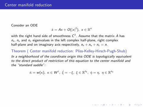
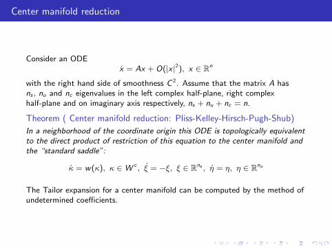
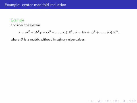
Example: center manifold reduction
Example
Consider the system
x = ax2 + xbT y + cx3 + . . . , x ∈ R1, y = By + dx2 + . . . , y ∈ Rm.
where B is a matrix without imaginary eigenvalues.
The Taylor expansion fora center manifold should have form
y = σx2 + O(x3)
with yet unknown vector coefficient σ.Plugging this y into the second equation of the system, we get
2σx(ax2 + xbT y + cx3 + . . .) + . . . = B(σx2 + O(x3)) + dx2 + . . .
Equating terms of order x2 we get Bσ + d = 0. Thus σ = −B−1d .Reduced onto the center manifold equation is
x = ax2 + (c − bTBd)x3 + O(x4).
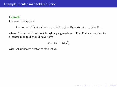
Example: center manifold reduction
Example
Consider the system
x = ax2 + xbT y + cx3 + . . . , x ∈ R1, y = By + dx2 + . . . , y ∈ Rm.
where B is a matrix without imaginary eigenvalues. The Taylor expansion fora center manifold should have form
y = σx2 + O(x3)
with yet unknown vector coefficient σ.
Plugging this y into the second equation of the system, we get
2σx(ax2 + xbT y + cx3 + . . .) + . . . = B(σx2 + O(x3)) + dx2 + . . .
Equating terms of order x2 we get Bσ + d = 0. Thus σ = −B−1d .Reduced onto the center manifold equation is
x = ax2 + (c − bTBd)x3 + O(x4).
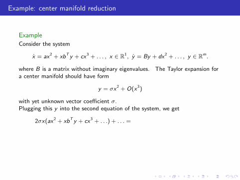
Example: center manifold reduction
Example
Consider the system
x = ax2 + xbT y + cx3 + . . . , x ∈ R1, y = By + dx2 + . . . , y ∈ Rm.
where B is a matrix without imaginary eigenvalues. The Taylor expansion fora center manifold should have form
y = σx2 + O(x3)
with yet unknown vector coefficient σ.Plugging this y into the second equation of the system, we get
2σx(ax2 + xbT y + cx3 + . . .) + . . . =
B(σx2 + O(x3)) + dx2 + . . .
Equating terms of order x2 we get Bσ + d = 0. Thus σ = −B−1d .Reduced onto the center manifold equation is
x = ax2 + (c − bTBd)x3 + O(x4).
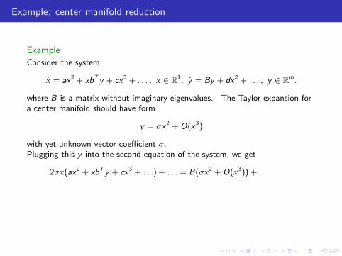
Example: center manifold reduction
Example
Consider the system
x = ax2 + xbT y + cx3 + . . . , x ∈ R1, y = By + dx2 + . . . , y ∈ Rm.
where B is a matrix without imaginary eigenvalues. The Taylor expansion fora center manifold should have form
y = σx2 + O(x3)
with yet unknown vector coefficient σ.Plugging this y into the second equation of the system, we get
2σx(ax2 + xbT y + cx3 + . . .) + . . . = B(σx2 + O(x3)) +
dx2 + . . .
Equating terms of order x2 we get Bσ + d = 0. Thus σ = −B−1d .Reduced onto the center manifold equation is
x = ax2 + (c − bTBd)x3 + O(x4).
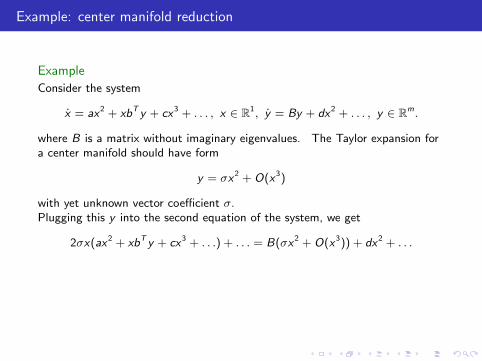
Example: center manifold reduction
Example
Consider the system
x = ax2 + xbT y + cx3 + . . . , x ∈ R1, y = By + dx2 + . . . , y ∈ Rm.
where B is a matrix without imaginary eigenvalues. The Taylor expansion fora center manifold should have form
y = σx2 + O(x3)
with yet unknown vector coefficient σ.Plugging this y into the second equation of the system, we get
2σx(ax2 + xbT y + cx3 + . . .) + . . . = B(σx2 + O(x3)) + dx2 + . . .
Equating terms of order x2 we get Bσ + d = 0. Thus σ = −B−1d .Reduced onto the center manifold equation is
x = ax2 + (c − bTBd)x3 + O(x4).
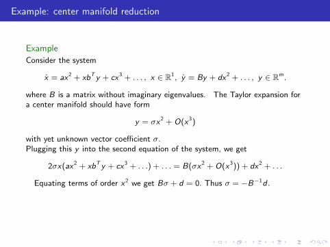
Example: center manifold reduction
Example
Consider the system
x = ax2 + xbT y + cx3 + . . . , x ∈ R1, y = By + dx2 + . . . , y ∈ Rm.
where B is a matrix without imaginary eigenvalues. The Taylor expansion fora center manifold should have form
y = σx2 + O(x3)
with yet unknown vector coefficient σ.Plugging this y into the second equation of the system, we get
2σx(ax2 + xbT y + cx3 + . . .) + . . . = B(σx2 + O(x3)) + dx2 + . . .
Equating terms of order x2 we get Bσ + d = 0. Thus σ = −B−1d .
Reduced onto the center manifold equation is
x = ax2 + (c − bTBd)x3 + O(x4).
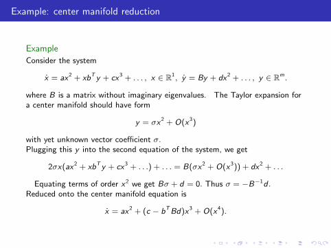
Example: center manifold reduction
Example
Consider the system
x = ax2 + xbT y + cx3 + . . . , x ∈ R1, y = By + dx2 + . . . , y ∈ Rm.
where B is a matrix without imaginary eigenvalues. The Taylor expansion fora center manifold should have form
y = σx2 + O(x3)
with yet unknown vector coefficient σ.Plugging this y into the second equation of the system, we get
2σx(ax2 + xbT y + cx3 + . . .) + . . . = B(σx2 + O(x3)) + dx2 + . . .
Equating terms of order x2 we get Bσ + d = 0. Thus σ = −B−1d .Reduced onto the center manifold equation is
x = ax2 + (c − bTBd)x3 + O(x4).
Center manifold reduction for systems with parameters
Consider an ODE (actually, k-parametric family of ODE’s)
x = v(x , α), v = A(α)x + O(|x |2), x ∈ Rn, α ∈ Rk
with the right hand side of smoothness C 2. Assume that the matrix A(0) hasns , nu and nc eigenvalues in the left complex half-plane, right complexhalf-plane and on imaginary axis respectively, ns + nu + nc = n.
Consider the extended system
x = v(x , α), α = 0
This system has in a neighborhood of the origin of the coordinates (x , α) acenter manifold of dimension nc + k.
Theorem ( Shoshitaishvili reduction principle)
In a neighborhood of the coordinates’ origin this ODE is topologicallyequivalent to the direct product of restriction of this equation to the centermanifold and the “standard saddle”:
κ = w(κ, α), κ ∈ Rnc , α = 0, α ∈ Rk , ξ = −ξ, ξ ∈ Rns , η = η, η ∈ Rnu
The homeomorphism which realizes equivalence does not change α.
The restriction of the original family ODE’s to the central manifold of theextended system is called the reduced family. According to the reductionprinciple in the problem of the topological classification without loss ofgenerality one may consider only reduced families.
Some definitions in bifurcation theory
The phase portrait of a dynamical system is a partitioning of the state spaceinto orbits.
Consider a dynamical system that depends on parameters (actually, family ofdynamical systems).
The appearance of a topologically nonequivalent phase portraits under variationof parameters is called a bifurcation.
A bifurcation diagram of the dynamical system is a stratification of itsparameter space induced by the topological equivalence, together withrepresentative phase portraits for each stratum.
A bifurcation boundary is a surface in the parameter space on which abifurcation occurs.
If family of dynamical systems is generic, then the codimension of a bifurcationis the difference between the dimension of the parameter space and thedimension of the corresponding bifurcation boundary. The codimension ofthe bifurcation of a given type is the minimal number of parameters of familiesin which that bifurcation type occurs. Equivalently, the codimension is thenumber of equality conditions that characterize a bifurcation.
Some definitions in bifurcation theory
The phase portrait of a dynamical system is a partitioning of the state spaceinto orbits.
Consider a dynamical system that depends on parameters (actually, family ofdynamical systems).
The appearance of a topologically nonequivalent phase portraits under variationof parameters is called a bifurcation.
A bifurcation diagram of the dynamical system is a stratification of itsparameter space induced by the topological equivalence, together withrepresentative phase portraits for each stratum.
A bifurcation boundary is a surface in the parameter space on which abifurcation occurs.
If family of dynamical systems is generic, then the codimension of a bifurcationis the difference between the dimension of the parameter space and thedimension of the corresponding bifurcation boundary.
The codimension ofthe bifurcation of a given type is the minimal number of parameters of familiesin which that bifurcation type occurs. Equivalently, the codimension is thenumber of equality conditions that characterize a bifurcation.
Some definitions in bifurcation theory
The phase portrait of a dynamical system is a partitioning of the state spaceinto orbits.
Consider a dynamical system that depends on parameters (actually, family ofdynamical systems).
The appearance of a topologically nonequivalent phase portraits under variationof parameters is called a bifurcation.
A bifurcation diagram of the dynamical system is a stratification of itsparameter space induced by the topological equivalence, together withrepresentative phase portraits for each stratum.
A bifurcation boundary is a surface in the parameter space on which abifurcation occurs.
If family of dynamical systems is generic, then the codimension of a bifurcationis the difference between the dimension of the parameter space and thedimension of the corresponding bifurcation boundary. The codimension ofthe bifurcation of a given type is the minimal number of parameters of familiesin which that bifurcation type occurs. Equivalently, the codimension is thenumber of equality conditions that characterize a bifurcation.
Exercises
Exercises
1. Consider the system
x = xz − x3, y = y + x4, z = 0
Show that this system has a center manifold given by y = V (x , z) , where V isa C 6 function in x if |z | < 1/6, but only a C 4 function in x for |z | < 1/4.
2. Consider the system
x = ax2 +xbT y +cx3 + . . . , x ∈ R1, y = By +dx2 +px3 +xqT y + . . . , y ∈ Rm.
where B is a matrix without imaginary eigenvalues. Find center manifold of 0with accuracy O(x4).

Bibliography
Arnold, V.I. Ordinary differential equations. Springer-Verlag, Berlin, 2006.
Arnold, V. I. Geometrical methods in the theory of ordinary differentialequations. Springer-Verlag, New York, 1988.
Arnold, V. I. Mathematical methods of classical mechanics. Springer-Verlag,New York, 1989.
Arrowsmith, D. , Place, C. An introduction to dynamical systems, CambridgeUniversity Press, Cambridge, 1990.
Dynamical systems. I, Encyclopaedia Math. Sci., 1, Springer-Verlag, Berlin,1998.
Guckenheimer, J. Holmes, P . Nonlinear oscillations, dynamical systems andbifurcations of vector fields, Springer-Verlag, Berlin, 1990.
Ilyashenko, Yu., Weigu Li, Nonlocal Bifurcations, AMS, 1999.
Hartman, P. Ordinary differential equations. (SIAM), Philadelphia, PA, 2002.
Kuznetsov, Yu.A. Elements of applied bifurcation theory. Springer-Verlag, NewYork, 2004.
Shilnikov, L. P.; Shilnikov, A. L.; Turaev, D. V.; Chua, L. O. Methods ofqualitative theory in nonlinear dynamics. Part I. World Scientific, Inc., RiverEdge, NJ, 1998.


![MATH 614, Spring 2016 [3mm] Dynamical Systems …Dynamical Systems and Chaos Lecture 1: Examples of dynamical systems. A discrete dynamical system is simply a transformation f : X](https://img.pdfslide.us/doc/110x75/5fc3a613bb041d25ed5cc331/math-614-spring-2016-3mm-dynamical-systems-dynamical-systems-and-chaos-lecture.jpg)