Lecturer: Dmitri A. Moltchanov E-mail: …Ad hoc networks D.Moltchanov, TUT, 2009 OUTLINE: Introduction Classi cation Proactive routing protocols Reactive routing protocols Hybrid

Routing protocols for ad hoc networks

Lecturer: Dmitri A. Moltchanov

E-mail: [email protected]

http://www.cs.tut.fi/kurssit/TLT-2756/

Ad hoc networks D.Moltchanov, TUT, 2009

OUTLINE:

• Introduction

• Classification

• Proactive routing protocols

• Reactive routing protocols

• Hybrid routing protocols

• Hierarchial routing protocols

• Power-aware routing protocols

Lecture: Routing protocols for ad hoc networks 2


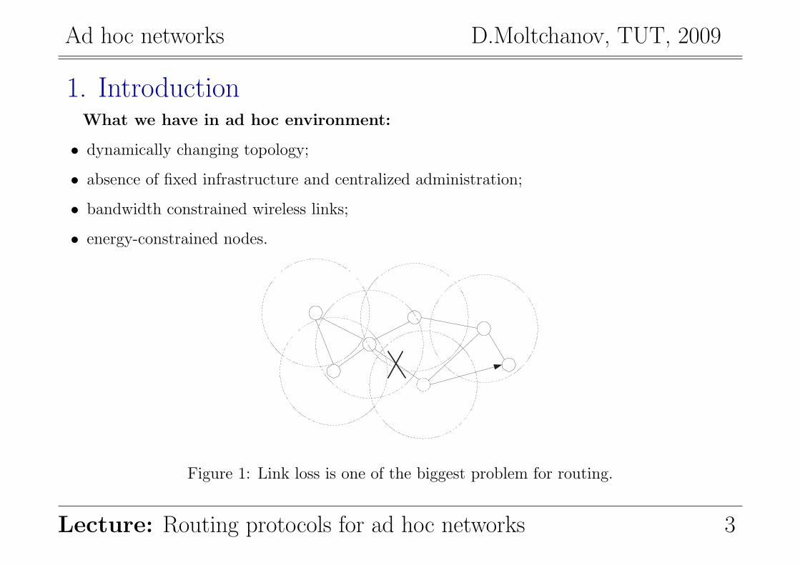
1. IntroductionWhat we have in ad hoc environment:

• dynamically changing topology;

• absence of fixed infrastructure and centralized administration;

• bandwidth constrained wireless links;

• energy-constrained nodes.

Figure 1: Link loss is one of the biggest problem for routing.



1.1. Challenges of routing protocols in ad hoc networks

The following are the main challenges:

• Movement of nodes:

– Path breaks;

– Partitioning of a network;

– Inability to use protocols developed for fixed network.

• Bandwidth is a scarce resource;

– Inability to have full information about topology;

– Control overhead must be minimized.

• Shared broadcast radio channel:

– Nodes compete for sending packets;

– Collisions.

• Erroneous transmission medium:

– Loss of routing packets.



1.2. Design goals

Goals that must be met:

• must be scalable;

• must be fully distributed, no central coordination;

• must be adaptive to topology changes caused by movement of nodes;

• route computation and maintenance must involve a minimum number of nodes;

• must be localized, global exchange involves a huge overhead;

• must be loop-free;

• must effectively avoid stale routes;

• must converge to optimal routes very fast;

• must optimally use the scare resources: bandwidth, battery power, memory, computing;

• should provide QoS guarantees to support time-sensitive traffic.



2. Classification of routing protocolsRouting protocols for ad-hoc wireless networks can be classified based on:

• routing information update mechanism;

• usage of temporal information (e.g. cached routes);

• usage of topology information;

• usage of specific resources (e.g. GPS).



Based on routing information update mechanism

• Proactive (table-driven) routing protocols;

• Reactive (on-demand) routing protocols;

• Hybrid protocols.

Based on usage of temporal information

• Based on past temporal information;

• Based on future temporal information.

Based on the routing topology

• Flat topology routing protocols:

• Hierarchial topology routing protocols:

Routing based on utilization of specific resources:

• Power-aware routing;

• Geographical information assisted routing.



Routing protocols for ad-hoc networks

Routing information update Temporal information for routing

HybridReactiveProactive Past history Predictions

- DSDV;

- WRP;

- CGSR;

- STAR;

- OLSR;

- FSR;

- HSR;

- GSR.

- DSR;

- AODV;

- ABR;

- SSA;

- FORP;

- PLBR.

- CEDAR;

- ZRP;

- ZHLS.

- DSDV;

- WRP;

- STAR;

- DSR;

- AODV;

- FSR;

- HSR;

- GSR.

- FORP;

- RABR;

- LBR.

Figure 2: Classification of routing protocols, part I.



Routing protocols for ad-hoc networks

Utilization of specific resource Topology information

FloodingGeographicalPower-aware Flat Hierarchial

- PAR. - LAR. - DSR;

- AODV;

- ABR;

- SSA;

- FORP;

- PLBR.

- CGSR;

- FSR;

- HSR.

Proactive Reactive

- OLSR. - PLBR.

Figure 3: Classification of routing protocols, part II.



3. Proactive routing protocolsThese are table-driven protocols.

We consider:

• destination sequenced distance vector routing protocol (DSDV);

• wireless routing protocol (WRP);

• cluster head gateway routing protocol (CGCR).

• source-tree adaptive routing protocol (STAR);

Common advantages and shortcoming of these protocols:

• +: low delay of route setup process: all routes are immediately available;

• −: high bandwidth requirements: updates due to link loss leads to high control overhead;

• −: low scalability: control overhead is proportional to the number of nodes;

• −: high storage requirements: whole table must be in memory.



3.1. Destination sequenced distance vector routing protocol (DSDV)

Modification of the Bellman-Ford algorithm where each node maintains:

• the shortest path to destination;

• the first node on this shortest path.

This protocol is characterized by the following:

• routes to destination are readily available at each node in the routing table (RT);

• RTs are exchanged between neighbors at regular intervals;

• RTs are also exchanged when significant changes in local topology are observed by a node.

RT updates can be of two types:

• incremental updates:

– take place when a node does not observe significant changes in a local topology;

• full dumps:

– take place when significant changes of local topology are observed;



13

2

4

6

5

Dest Next Dist

6

5

3

3 2

2

4 2 2

Figure 4: Example of routing table in DSDV.

The reconfiguration of path (used for ongoing data transfer) is done as follows:

• the end node of the broken link sends a table update message with:

– broken link’s weight assigned to infinity;

– sequence number greater than the stored sequence number for that destination.

• each node re-sends this message to its neighbors to propagate the broken link to the network;

• even sequence number is generated by end node, odd – by all other nodes.

Note: single link break leads to the propagation of RT updates through the whole network!



13

2

4

6

5

Dest Next Dist

6

5

3

3 2

3

4 2 2

13

2

465

Figure 5: Route update in DSDV.

Route maintenance in DSDV is performed as follows:

• when a neighbor node perceives a link break (node 3):

– it sets all routes through broken link to ∞;

– broadcasts its routing table.

• node 5 receives update message, it informs neighbors about the shortest distance to node 6;

• this information is propagated through the network and all node updates their RTs;

• node 1 may now sends their packets through route 1− 3− 5− 6 instead of 1− 3− 6.



3.2. Wireless routing protocol (WRP)

Each node maintains the following:

• Distance table (DT) containing network view of the neighbors of the node:

– distance and predecessor node for all destinations as seen by each neighbor.

• Routing table (RT) containing view of the network for all known destinations including:

– the shortest distance to destinations;

– the predecessor node;

– the successor node;

– flag indicating the status of the path (correct, loop, null).

• Link cost table (LCT) containing cost-related information including:

– number of hops to reach destination (cost of the broken link is ∞);

– number of update periods passed from the last successful update of the link.

• Message retransmission list (MRL) containing counter for each entry:

– the counter is decremented after every retransmission of the update message.



13

24

6

5

Dest Next Pred

7

6

7

3 5

7

5 7 5

7

Source

Destination

4

3

2

1

Cost

2 4

71

2

34

3

2

32

7

5

7

3

4

5

2

5

2

4

3

6

0

8

3

Routing entries at each node for destination 7:

Figure 6: Routing table in WRP.

Break: detected by number of update periods missed since successful transmission:

• each update message contains a list of updates;

• a node marks each node in RT that has to acknowledge update message it transmitted;

• once the counter of MRL reaches zero:

– entries in update message for which no acknowledgement received are to be retransmitted;

– update message is deleted.



When a node detects a link break:

• it sends an update message to its neighbors with link cost set to ∞;

• all affected node update their routes when they receive update message;

• the node that initiated the update message finds an alternative route from its DT;

• it updates its RT and sends update message to its neighbors;

• nodes update its RTs if this received route is better than they have, otherwise they discard it.

13

2

4

6

5

Dest Next Pred

7

6

7

3 4

7

5 4 4

7

Source

Destination

4

3

2

1

Cost

2 4

71

2

3

4

3

2

32

7

4

7

2

4

4

2

2

2

5

3

7

0

9

4

Dest Next Pred

7

6

7

3 5

7

5 7 5

4

3

2

1

Cost

7

5

7

3

4

5

2

5

2

4

3

6

0

8

3

Figure 7: Route maintenance in WRP.



3.3. Cluster head gateway switch routing protocol (GGSR)

It is characterized by the following:

• nodes are organized into clusters, each having an elected cluster-head;

• cluster head provides a coordination within its transmission range (single hop);

• token-based scheduling is used within a cluster for sharing bandwidth between nodes;

• all communications pass through the cluster head;

• communication between cluster is done using the common nodes (gateways with two interfaces).

D

S

Figure 8: Abstract representation of routing in GGSR.



Two tables are used in CGSR:

• Cluster member table containing the destination cluster head for every node;

• Routing table containing the next-hop node for every destination cluster.

The protocol operates as follows:

• a node obtains a token from its cluster head;

• if this node has a packet to transmit, it determines the destination cluster head and next-hop;

• routed packet goes as follows:

– a−H1 −G1 −H2 −G2 − · · · −Hi −Gi − · · · −Gn −Hn − b: where

– Gi is the gateway i;

– Hi is the cluster head i.

Route reconfiguration happens when:

• there is a change in cluster heads;

• stale entries are in cluster member table or routing table.



3

4

6

5

7

Source

Destination

8

9

1

10

2

11

12

13

14

15

Gateway node

Cluster head

Source and destination

Figure 9: Route path in CGSR.



3.4. Source-tree adaptive routing protocol (STAR)

There are two protocols with different aims:

• Least overhead routing approach (LORA):

– minimize control overhead irrespective of optimality;

• Optimum routing approach (ORA):

– provide optimal routes irrespective of the control overhead;

The STAR protocol operates as follows:

• each node is required to:

– send an update message to its neighbors during initialization;

– send update messages about new destinations, chances of routing loops, costs of paths.

• every node broadcasts its source-tree information:

– wireless links used by the node in its preferred path to destinations.

• every node builds its partial graph of topology based on:

– its adjacent links with neighbors, source-tree broadcasts by neighbors.



3

2

415

6

8

7

3

2

415

6

8

7

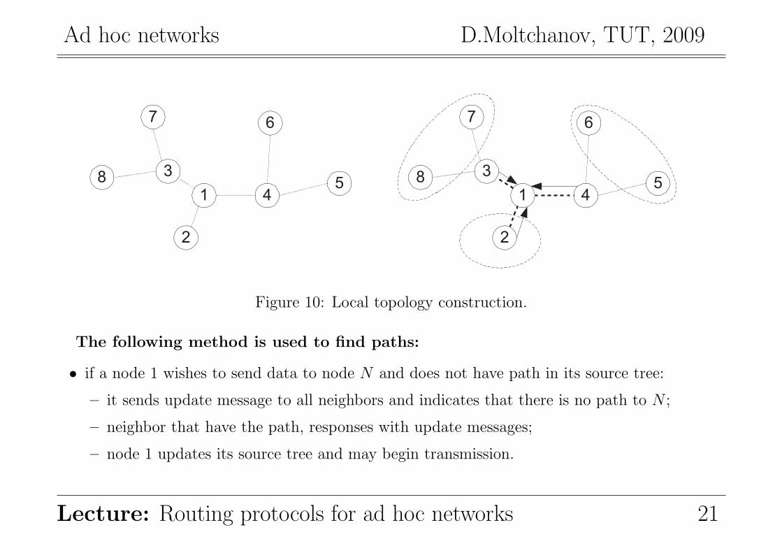
Figure 10: Local topology construction.

The following method is used to find paths:

• if a node 1 wishes to send data to node N and does not have path in its source tree:

– it sends update message to all neighbors and indicates that there is no path to N ;

– neighbor that have the path, responses with update messages;

– node 1 updates its source tree and may begin transmission.



4. Reactive routing protocolsThese protocols find paths to destination only when needed (on-demand) to transmit a packet.

We consider:

• Dynamic source routing protocol (DSR);

• Ad hoc on-demand distance vector routing protocol (AODV);

• Location aided routing (LAR);

• Associativity-based routing (ABR);

• Signal stability-based adaptive routing protocol (SSA);

These protocols have the following advantages and shortcomings:

• −: high delay of route setup process: routes are established on-demand;

• +: small control overhead: no route updates;

• −: low scalability: no route updates;

• −: low storage requirements: only needed routes are in cache.



4.1. Dynamic source routing protocol

This is a source-based routing protocol.

The difference between DSR and other on-demand routing protocols is:

• on-demand protocols periodically exchange the so-called beacon (hello) packets:

– hello packets are used to inform neighbors about existence of the node.

• DSR does not use hello packets.

The basic approach of this protocol is as follows:

• during route contraction DSR floods a RouteRequest packets in the network;

• intermediate nodes forward RouteRequest if it is not redundant;

• destination node replies with RouteReply;

• the RouteReply packet contains the path traversed by RouteRequest packet;

• the receiver responds only if this is a first RouteRequest (not duplicate).



The DSR protocol uses the sequence numbers:

• RouteRequest packet carries the path traversed and the sequence number;

• the sequence numbers are used to prevent loop formation and nodes check it.

The DSR also uses route cache in each node:

• if node has a route in the cache, this route is used.

10

9

2

4

6

5

R12

8

S14

13

16

7

Figure 11: Route establishment in DSR.



Refinements of DSR:

• to avoid over-flooding the network, exponential back-off is used between RouteRequest sending;

• intermediate node is allowed to reply with RouteReply if it has a route to destination in cache:

• if the link is broken the RouteError is sent to the sender by node adjacent to a broken link.

1

7

5

4

9

2

3

86

Figure 12: Route failure notification in DSR.



4.2. Ad hoc on-demand distance vector routing protocol

The major differences between AODV and DSR are as follows:

• in DSR a data packet carries the complete path to be traversed;

• in AODV nodes store the next hop information (hop-by-hop routing) for each data flow.

The RouteRequest packet in AODV carries the following information:

• the source identifier (SrcID): this identifies the source;

• the destination identifier (DestID): this identifies the destination to which the route is required;

• the source sequence number (SrcSeqNum);

• the destination sequence number (DestSeqNum): indicates the freshness of the route.

• the broadcast identifier (BcastID): is used to discard multiple copies of the same RouteRequest.

• the time to live (TTL): this is used to not allow loops.



The AODV protocol performs as follows:

• when a node does not have a valid route to destination a RouteRequest is forwarded;

• when intermediate node receives a RouteRequest packet two cases are possible:

– if it does not have a valid route to destination, the node forwards it;

– if it has a valid route, the node prepares a RouteReply message:

• if the RouteRequest is received multiple times, the duplicate copies are discarded:

– are determined comparing BcastID-SrcID pairs.

• when RouteRequest is forwarded, the address of previous node and its BcastID are stored;

– are needed to forward packets to the source.

• if RouteReply is not received before a time expires, this entry is deleted;

• either destination node or intermediate node responses with valid route;

• when RouteRequest is forwarded back, the address of previous node and its BcastID are stored;

– are needed to forward packets to the destination.



1

7

5

4

9

2

S

86

1211

10

13

14

R

16

17RouteRequest:

- DestSeqNum:5,

- SrcSeqNum: 2

Node 8:

- DestSeqNum 3;

Node 9:

- DestSeqNum 7;

Figure 13: Route establishment in AODV.



In case of the link break:

• end-node are notified by unsolicited RouteReply with hop count set to ∞;

• end-node deletes entries and establishes a new path using new BcastID;

• link status is observed using the link-level beacons or link-level ACKs.

1

7

5

4

9

2

S

86

1211

10

13

14

D

16

17

Figure 14: Route maintenance in AODV.



4.3. Location aided routing

What are basics of LAR:

• uses the location information (assumes the availability of GPS);

• reactive (on-demand) protocol.

LAR designates two zones for selective forwarding of control packets:

• ExpectedZone:

This is a geographical zone in which the location of the terminal is predicted based on:

– location of the terminal in the past;

– mobility information of the terminal.

There is no info about previous location of the terminal the whole network is the ExpectedZone.

• RequestZone:

This is a geographical zone within which control packets are allowed to propagate:

– this area is determined by the sender of the data packet;

– control packets are forwarded by node within a RequestZone only;

– if the node is not found using the first RequestZone, the size of RequestZone is increased.



8

5

6

7

2

9

4

1

3

Source

Dest.

10

3

Figure 15: Example of ExpectedZone and RequestZone.

Nodes decide whether to forward or discard packets based on two algorithms:

• LAR type 1;

• LAR type 2.



LAR type 1 algorithm works as follows:

• the sender explicitly specifies the RequestZone in the RouteRequest packet;

• the RequestZone is the smallest rectangle that includes the source and the ExpectedZone;

• when the node is in ExpectedZone, the RequestZone is reduced to the ExpectedZone;

• if the ReouteRequest packet is received by the node within RequestZone, it forwards it.

8

5

6

7

2

9

4

1

3

Source

Dest.

10

3

Figure 16: Routing procedure in LAR type 1.



LAR type 2 algorithm operates as follows:

• the sender includes the distance to the source in the RouteRequest packet;

• intermediate nodes compute the distance to the destination:

– if this distance is less than the distance between source and destination packet is forwarded;

– otherwise the packet is discarded.

• distance in the packet is updated at every node with lower distance to destination.

8

5

6

7

2

9

4

1

3

Source

Dest.

10

11

12

13

14

15

16

18

17

Figure 17: Routing procedure in LAR type 2.



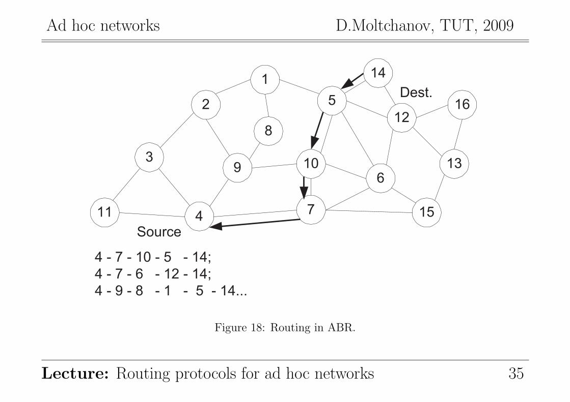
4.4. Associativity-based routing

It is characterized by the following:

• on-demand beacon-based protocol;

• routes are selected based on temporal stability of wireless links:

• to determine temporal stability, each node maintains the count of its neighbors’ beacons.


• source node floods the RouteRequest packet, all intermediate nodes forward this packet;

• RouteRequest packet carries the following:

– the path it has traversed;

– the beacon count for corresponding node in the path.

• when the first RouteRequest reaches the destination, the destination:

– waits for RouteSelect time to receive multiple copies of RouteRequest;

– selects the path that has the maximum number of stable links;

– replies to the source with RouteReply packet.



8

5

6

7

2

9

4

1

3

Source

Dest.

10

11

12

13

14

15

16

4 - 7 - 10 - 5 - 14;

4 - 7 - 6 - 12 - 14;

4 - 9 - 8 - 1 - 5 - 14...

Figure 18: Routing in ABR.



If the link break occurs:

• the node closer to the source initiates a local link repair as follows:

– broadcasts locally route repair packet (local query (LQ)) with limited TTL (e.g., 3);

• if this node fails to repair, then the next node closer to destination initiates a route repair;

• if nodes constituting a half of pass of the route fail to repair, the source is informed.

8

5

6

7

2

9

4

1

3

Source

Dest.

10

11

12

13

14

15

16

Figure 19: Local route repair in ABR.



4.5. Signal stability-based adaptive routing protocol

This protocol is characterized by the following:

• on-demand beacon-based protocol;

• routes are selected based on temporal stability of wireless links:

• based on temporal stability, each links is classified to:

– stable

– unstable

• to determine temporal stability, each node measures the signal strength of beacons.

The whole protocols consist of the following two parts:

• dynamic routing protocol (DRP):

– DRP maintains the routing table interacting with DRPs on other hosts.

• forwarding protocol (FP):

– is responsible for forwarding of packets to destination.



In each node the signal stability table is maintained containing:

• beacon count and signal strength of these beacons;

– if the signal strength is strong for past few beacons the link is stable;

– if the signal strength is weak for past few beacons the link is unstable.


• if no route in cache, the node floods the RouteRequest packet;

• RouteRequest packet carries the path it has traversed;

• if the intermediate node receives the RouteRequest via stable link it forwards it;

• if the intermediate node receives the RouteRequest via unstable link it drops it;

• when the first RouteRequest reaches the destination, the destination:

– waits for RouteSelect time to receive multiple copies of RouteRequest;

– selects the path that is most stable;

∗ if two or more paths are equal in stability, the shortest path is selected;

∗ if two or more shortest paths are available, random path among them is selected.

– replies to the source with RouteReply packet.



8

5

6

7

2

9

4

1

3

Source

Dest.

10

11

12

13

14

15

16

4 - 7 - 10 - 5 - 14;

4 - 7 - 10 - 5 - 12 - 14.

Figure 20: Routing in SSA.



In case of the link break:

• end-nodes are informed and they try to establish new stable route;

• of no stable routes are available, the restriction of stable links is removed.

8

5

6

7

2

9

4

1

3

Source

Dest.

10

11

12

13

14

15

16

4 - 7 - 10 - 5 - 14;

4 - 7 - 10 - 5 - 12 - 14.

Figure 21: Route repair in SSA.



4.6. Flow-oriented routing protocol

Aim is on supporting real-time traffic using a predictive multi-hop-handoff feature:

• Classic protocols (e.g., DSR, AODV etc.):

– route repair is initiated when intermediate node detects the link breaks;

– it causes delay, losses: low QoS is provided in result.

• FORP uses the predictive mechanism to estimate link expiration time (LET):

– it is based on location, mobility and transmission range of nodes involved in forwarding;

– the minimum of LET determines the route expiration time (RET);

– it is assumed that GPS is used to make prediction of LET.

New shortcomings:

• −: devises are expensive;

• −: can only operate at the open air (due to GPS).




• if no route in cache, the destination floods the Flow-REQ packet carrying:

– information regarding the source and destination nodes;

– flow identification number (sequence number) that is unique for every session.

• when neighbor receives the Flow-REQ packet:

– to avoid looping checks if the sequence number if higher than that previously used;

– if so, this node appends LET and its address in the packet, and forwards it;

– if not, the packet is discarded.

• when the destination receives the packet:

– the packet has a path it has traversed and LET associated with each wireless link;

– if RET is acceptable, it originates the Flow-SETUP packet.

• when the source receives Flow-SETUP packet, it begins the transmission of packets.



8

5

6

7

2

9

4

1

3

Source

Dest.

10

11

12

13

14

15

16

4 - 7 - 10 - 5: RET: 8

4 - 9 - 8 - 1 - 5: RET: 5

10

8

14 9

17

7

5

Figure 22: Route establishment in FORP.



The LET of the link is estimated as follows:

LETAB =−(pq + rs) + (p2 + r2)T 2

X − (ps− qr)2

p2 + q2,

p = VA cosTA − VB cosTB, q = XA −XB

r = VA sinTA − VB sinTB, s = YA − YB, (1)

• A and B are nodes with transmission range TX ;

• VA and VB are velocities of nodes;

• TA and TB are angles as shown below:

A: (XA,Y

A) B: (X

B,Y

B)

TA

TB

Figure 23: Motion angles in FORM.



FORP uses proactive route maintenance using available RET:

• when the destination determines that the break is about to occur it sends Flow-HANDOFF;

• Flow-HANDOFF propagates in the network similarly to Flow-REQ;

• when many Flow-HANDOFF are received at the source new path with highest RET is chosen.

8

5

6

7

2

9

4

1

3

Source

Dest.

10

11

12

13

14

15

16

10

8

14 9

17

7

5

5 - 10 - 7 - 4: RET: 5

5 - 1 - 8 - 9 - 4: RET: 8

5 - 1 - 3 - 4: RET: 3

5 - 6 - 7 - 4: RET: 7

7

9

3

5

6

Figure 24: Route repair in FORP.



5. Hybrid routing protocolsThese protocols maintain topology information up to m hops in tables.

We consider:

• Zone routing protocol (ZRP);

• Zone-based hierarchial link state routing protocol (ZHLS);

What are inherent shortcomings and advantages:

• +: fast link establishment;

• +: less overhead as compared to table-driven and reactive protocols.

• −: high storage and processing requirements as compared to reactive protocols.

Note: a compromise between proactive and reactive protocols.



5.1. Zone routing protocol (ZRP)

This protocols uses a combination of proactive and reactive routing protocols:

• proactive: in the neighborhood of r hops: Intra-zone routing protocol (IARP);

• reactive: outside this zone: Inter-zone routing protocol (IERP).

8

5

6

7

2

9

4

1

3

Source

Dest.

10

11

12

13

14

15

16

r = 2

r = 1

For r = 2:

5, 6, 7, 9 are interior nodes

14, 12, 15, 4, 2, 8, 1 are paripheral nodes

Routing within a zone toplogy information

is exchanged using route update packets.

Figure 25: Zones in ZRP for node 10.




• if the destination is within the zone, the source sends packets directly;

• if not, the destination sends RouteRequest to peripheral nodes;

• if any peripheral node, has the destination in its zone it replies with RouteReply;

• if not, peripheral nodes sends RouteRequest to their peripheral nodes and so on;

• if multiple RouteReply are received the best is chosen based on some metric.

If the broken link is detected:

• intermediate node repairs the link locally bypassing it (proactive routing!!!);

• end nodes are informed;

• sub-optimal pass but very quick procedure;

• after several local reconfiguration, the source initiates global pass finding to find optimal.



8

5

6

7

2

9

4

1

3

Dest.

Source

10

11

12

13

14

15

16

Figure 26: Routing in ZRP with r = 1.



5.2. Zone-based hierarchial link state routing protocol

ZHLS is characterized by the following:

• use of geographical location of nodes to determine the non-overlapping zones;

• hierarchial addressing with zone ID and node ID is used;

• each node requires the location information based on which its zone is obtained;

• topology information is maintained in every node inside this zone;

• for regions outside the zone, zone connectivity information is maintained;

The ZHLS uses:

• proactive routing is used inside zone;

• reactive routing is used outside zone;

Note: ZHLS requires GPS or similar service to identify itself with a certain sone.

Zones: coverage of the single node, application scenario, mobility of nodes, network size.




• each node builds a one-hop node-level topology;

• this one-hop topology is propagated to other nodes in its zone using packet containing:

– IDs of all zones in the zone, node ID, and zone IDs of all other nodes.

• nodes that receive responses from nodes belonging to other zones are gateway nodes;

• all traffic between zones is transmitted via gateway nodes;

• once node-level topology is built, nodes obtain zone-level topology sending packets via gates;

• if the destination is in the zone, packets are forwarded directly;

• if no, the source sends location request packet to every zone via gateways;

• every gateway node checks for destination in its routing table and replies with ReouteReply.



8

5

6

7

2

9

4

1

310

11

12

13

14

15

16BCD A

EFGH

Figure 27: ZHLS zones.

The repair of broken links is as follows:

• source is notified about the link failures;

• if there are multiple gateways with the required zone, packet if forwarded via one of those;

• if no multiple gateways, packets are forwarded to other zones and then to the required zone.



6. Hierarchial routing protocolsThese protocols introduce hierarchy in the network to achieve the following benefits:

• reduction in the size of routing tables;

• better scalability.

6.1. Hierarchial state routing protocol

HSR is characterized by the following:

• HSR uses multi-clustering to enhance resource allocation and management;

• HSR defines different levels of clusters;

• at every level leader is elected;

• the first level is made of single-hop clusters (physical clustering);

• the next level is comprised of leaders of clusters.



8

5

6

7

2

9

4

310

11

12

13

15

16Level 0

17

18

19

20

Level 1

Level 2

Figure 28: Topology example in HSR.



At the physical layer nodes are classified into:

• cluster heads; belong to a single cluster and elected as a cluster head;

• gateway nodes; belong to two or more clusters;

• normal nodes: belong to a single cluster.

Cluster heads at level 0 (physical level) could be responsible for:

• slot/frequency/code allocation to utilize spectrum more efficiently;

• call admission control from normal member nodes;

• scheduling of packets for transmission;

• exchange of routing information;

• handling route breaks.

Gateway nodes are responsible for:

• forwarding of packets between different clusters (cluster heads).



The following routing responsibilities are assigned to nodes in HSR:

• every node maintains information about the status of links with its neighbors:

– this information is broadcasted within the cluster at regular intervals.

• cluster heads exchange the topology and link state information at any level:

– this is done via multiple hops using the gateway nodes.

• the path between two cluster head involves multiple links is called the virtual link:

– this is: head - gateway - head - gateway etc.

• every node knows the exact hierarchial topology information:

– after obtaining the information the cluster head floods it to lower level.

• to route packets hierarchial addressing is used consisting of;

– hierarchial ID (HID): sequence of cluster headers’ IDs from higher level;

– node ID: similar to unique MAC address.

Address of node 12: (9,12,12).

• From 12 to 3: 12 - 9 - 3 over multiple links.



6.2. Fisheye state routing protocol

Generalization of the GSR protocol where the following property is introduced:

• accurate information about nodes in local topology;

• not so accurate information about node that are far away.

Why is it needed:

• complexity proactive routing: size of the network, mobility of node;

• reactive routing: + number of connections.

What is the basis:

• a node exchanges the routing information only with neighbors at periodic intervals:

– trade-off between link-state (topology exchanges) and distance vector (link-level info).

• the complete topology information is maintained at each nodes;

• different update frequencies for different scopes one-hop/two-hop/... scopes:

– one-hop – highest freq., two-hop less freq. etc.: decrease of the message size.



8

5

6

7

2

9

4

310

11

12

13

15

16

17

18

19

20

Figure 29: One-hop and two-hop scopes of the node.

1

3

2

4

Dest. Neigh. Hops

1 2,3 0

2 1 1

3 1,4 1

4 3 2

one-hop neighbors

two-hop neighbors

Figure 30: Example of topology information in FSR.



7. Power-aware routing protocolsThe following metrics can be taken into account on route selection procedure:

• Minimal energy consumption per a packet:

This metric involves a number of nodes from source to destination.

– +: uniform consumption of power throughout the network;

• Maximize the network connectivity:

To balance the load between the cut-sets (those nodes removal of which causes partitions).

– −: difficult to achieve due to variable traffic origination.

• Minimum variance in node power levels:

To distribute load such that power consumption pattern remains uniform across nodes.

– +: nearly optimal performance is achieved by routing a packet to least loaded next-hop.

• Minimum cost per a packet:

Cost as a function of the battery charge (less energy – more cost) and use it as a metric.

– +: easy to compute (battery discharge patterns are available);

– +: this metric handles congestions in the network.


Documents

Lecturer: Dmitri A. Moltchanov E-mail: …Ad hoc networks D.Moltchanov, TUT, 2009 OUTLINE: Introduction Classi cation Proactive routing protocols Reactive routing protocols Hybrid